Mechanic: the MPI/HDF code framework for dynamical astronomy

Abstract

We introduce the Mechanic, a new open-source code framework. It is designed to reduce the development effort of scientific applications by providing unified API (Application Programming Interface) for configuration, data storage and task management. The communication layer is based on the well-established Message Passing Interface (MPI) standard, which is widely used on variety of parallel computers and CPU-clusters. The data storage is performed within the Hierarchical Data Format (HDF5). The design of the code follows core–module approach which allows to reduce the user’s codebase and makes it portable for single- and multi-CPU environments. The framework may be used in a local user’s environment, without administrative access to the cluster, under the PBS or Slurm job schedulers. It may become a helper tool for a wide range of astronomical applications, particularly focused on processing large data sets, such as dynamical studies of long-term orbital evolution of planetary systems with Monte Carlo methods, dynamical maps or evolutionary algorithms. It has been already applied in numerical experiments conducted for Kepler-11 (Migaszewski et al., 2012) and $\nu$Octantis planetary systems (Goździewski et al., 2013). In this paper we describe the basics of the framework, including code listings for the implementation of a sample user’s module. The code is illustrated on a model Hamiltonian introduced by (Froeschlé et al., 2000) presenting the Arnold diffusion. The Arnold Web is shown with the help of the MEGNO (Mean Exponential Growth of Nearby Orbits) fast indicator (Goździewski et al., 2008a) applied onto symplectic SABA_n integrators family (Laskar and Robutel, 2001).

1 Introduction

In the field of dynamical astronomy several numerical techniques have been proposed to determine the nature of the phase space of planetary systems. The Monte Carlo methods (e.g., Holman and Wiegert, 1999), evolutionary algorithms (e.g., Goździewski et al., 2008b; Goździewski and Migaszewski, 2009) or dynamical maps (e.g., Froeschlé et al., 2000; Guzzo, 2005; Migaszewski et al., 2012; Goździewski et al., 2013) have become standard research tools for determining possible or permitted configurations, mass ranges or other physical data. These experiments usually require intensive tests of sets of initial conditions, that represent different orbital configurations. They involve direct numerical integrations of equations of motion to study long-term orbital evolution. To characterize the dynamical stability of orbital models, so called fast chaos indicators are often used (e.g., Goździewski et al., 2008a). These numerical tools make it possible to resolve efficiently whether a given solution is stable (quasi-periodic, regular) or unstable (chaotic) by following relatively short parts of the orbits. The fast indicators, like the Fast Lyapunov Indicator (FLI, Froeschlé et al., 2000), the Frequency Map Analysis (FMA, Laskar, 1993; Sidlichovský and Nesvorný, 1996), the Mean Exponential Growth factor of Nearby Orbits (MEGNO, Cincotta and Simó, 2000; Cincotta et al., 2003; Mestre et al., 2011), the Spectral Number (SN, Michtchenko and Ferraz-Mello, 2001), are well known in the theory of dynamical systems (Barrio et al., 2009). In the past decade, they were intensively adapted to the planetary dynamics (e.g., Froeschlé et al., 1997; Robutel and Laskar, 2001; Goździewski et al., 2008a).

Depending on the dynamical model of a planetary system, its numerical setup and the chaos indicator used to represent the dynamical state, the simulation of a set of initial conditions may require large CPU resources. However, since each test may be understood as a separated numerical task, parallelization techniques may be used, with tasks distributed among available CPUs and evaluated in parallel. The basic approach relies on the task farm model, in which independent tasks are processed on worker nodes with the result collected by the master. From the technical point of view, this algorithm requires implementation of the CPU-communication layer, and should allow input preparation and result assembly for the post-processing. These issues are addressed in general-purpose distributed task management systems, like HTCondor (Fields, 1993), or Workqueue (Yu et al., 2010). Within such frameworks, the user-supplied, standalone executable code performing computations (application) is distributed over a computing pool. The input and output for each software instance is achieved via batch scripts (e.g. the Makeflow extension for the Workqueue package), making this approach application- and problem-dependent. This might be insufficient for large and long-term numerical tests, such as studying the dynamics of planetary systems. In particular, our recent work on Kepler-11 (Migaszewski et al., 2012) and $\nu$Octantis (Goździewski et al., 2013) systems required developing a new code framework, the Mechanic, dedicated to conducting massive parallel simulations. It has been turned out into general-purpose master–worker framework, built on the foundation of the Message Passing Interface (Pacheco, 1996). The Mechanic separates the numerical part of the user’s code (a module) from its configuration, communication and storage layers (a core). This partition is achieved through the provided Application Programming Interface (API). On the contrary to HTCondor and Workqueue packages, the task preparation and result data storage is handled by the core of the framework. The final result is assembled into one datafile, which reduces the cost of post-processing large simulations. The storage layer is built on top of the universal HDF5 data format (The HDF5 Group, 2012). No MPI nor HDF5 programming knowledge is required to use the framework, which makes it possible to parallelize “scalar” codes relatively easily. The Mechanic may be used both system-wide as well as in a local user’s environment under the control of job schedulers, such as PBS or Slurm.

This paper is structured as follows. We give a short overview of the Mechanic in Section 2. To explain programming concepts behind the framework we illustrate it with the help of the Hamiltonian model introduced by Froeschlé et al. (2000). It reveals the so called Arnold web, which represents a set of resonances of a quasi-integrable dynamical systems. It has been intensively studied in recent years (Cincotta, 2002; Lega et al., 2003; Guzzo et al., 2004; Froeschlé et al., 2005, 2006), and applied to study long-term evolution of the outer Solar System (Guzzo, 2005, 2006). In Section 3 we give short theoretical background on this topic. The very fine details of the phase space obtained with the dedicated module for the Mechanic are presented in the Section 4. The technical implementation of the module is given in the Appendix.

2 Overview of the framework

The Mechanic provides a skeleton code for common technical operations, including run-time configuration, memory and file management, as well as CPU communication. It has been developed to mimic the user’s application flow in a problem-independent way (Listing 1). This is achieved via provided API, which allows to reduce the user’s code to a module form, containing only its numerical part along with setup and storage specifications required to run it (Listing 2). The core of the framework loads the module dynamically during the runtime, performs the setup and storage stages according to these specs and executes the numerical part.

The benefit of this core–module approach comes both in data and task management. For instance, let us recall the concept of dynamical maps. The phase space of the dynamical system is mapped onto two-dimensional plane. Each point on that plane represents the dynamical state of the specific initial condition. From the technical point of view, computing the dynamical map requires execution of several numerical tasks that differs with the input, and assembling the result in an accessible way for post-processing. Assuming that each task (initial condition) is computed by a single instance of the application, the simulation requires preparing the input and collecting the result with the help of batch scripts. Although the HTCondor and Workqueue frameworks provide powerful task management tools, input and output data management is left to the user. The Mechanic framework works more like Makeflow (a Workqueue make engine), however, the user’s code connected to the core is treated as a whole application with single output datafile and the input that may be prepared programatically according to the information associated with the current task.

Listing 1: The internal design of the framework (pseudocode). The user’s code is connected with the framework through the provided API (hooks are marked with bold font face). API hooks used in the module are executed in a specific order to mimic the user’s application flow. The bootstrap stage involves Init() and Setup() hooks for code initialization. After that, the framework enters the task pool loop. For each task pool p, the information provided with the Storage() hook is used to allocate the required memory and the file storage. The PoolPrepare() hook allows to prepare the global data and configuration of the pool p. This hook has access to the data computed in the previous pools, if any. Each task pool p involves evaluation of the task loop. The set of numerical tasks is allocated on the core part, so that they are available for use in the API. For each task, the TaskPrepare() and TaskProcess() hooks are executed. The computed data is saved through the task t object that is passed to the hooks. In the case of the master–worker approach, the for loop showed in the listing is parallelized. The task t is initialized on the master node and sent to the worker. TaskPrepare() and TaskProcess() hooks are executed on the worker node, and the data of the task t is passed back to the master node and saved. After the task loop is completed, the PoolProcess() hook is used to determine whether to continue the task pool loop. To do so, the user may use the data stored in the previous pools, if any. During the framework execution, memory and file management, CPU-communication and data storage are performed on the core part without the need of user interaction.

⬇

Init()

Setup()

allocate task pools

// task pool loop:

do {

allocate new task pool p

Storage(p)

allocate tasks in the task pool p

PoolPrepare(pools, p)

// task loop:

for all t in tasks {

get the task t

TaskPrepare(p, t)

TaskProcess(p, t)

save the task t

}

new = PoolProcess(pools, p)

save task pool p in pools

} while (new == POOL_CREATE_NEW)

Listing 2: The sample module structure. Each API hook is provided with the information that is neccessary on the corresponding execution stage, such as pool and task configuration, through pool *p and task *t pointers. The default return code SUCCESS indicates the successful evaluation of the hook. Otherwise, the hook must return error code, as specified in the API documentation. This helps the framework to safely abort the simulation. The listing shows only the most essential API hooks. See the package documentation for the detailed list of hooks.

⬇

#include "mechanic.h"

int Init(init *i) {

return SUCCESS;

}

int Setup(setup *s) {

return SUCCESS;

}

int Storage(pool *p) {

return SUCCESS;

}

int PoolPrepare(pool **pools, pool *p) {

return SUCCESS;

}

int TaskPrepare(pool *p, task *t) {

return SUCCESS;

}

int TaskProcess(pool *p, task *t) {

return TASK_FINALIZE;

}

int PoolProcess(pool **pools, pool *p) {

return POOL_FINALIZE;

}

The base master–worker algorithm with single input and output may be easily implemented with the minimum knowledge on the MPI programming. However, the purpose of the Mechanic is to reduce this development effort. With the help of the API, the user’s code is separated from the task management layer. It allows to use different communication patterns between nodes in a computing pool (cluster) without modification of the module. In addition to the master–worker pattern, the master-only mode without MPI communication is provided, which behaves similar to a single-CPU application. Moreover, the API allows to implement different communication patterns, if required by the user’s code.

The task assignment is performed within multidimensional grid and is governed through the API. Although this suits best the concept of dynamical maps, the API has been designed to support different assignment patterns, such as Monte Carlo methods. The key design concept of the Mechanic is a task pool. It represents a set of numerical tasks to perform for a particular setup (i.e. single dynamical map). The framework allows to create task pools dynamically depending on the results, with different configuration, storage and number of tasks. This helps to implement evolutionary algorithms and processing pipelines despite of number of CPUs involved in the simulation.

The result data, among with the run-time configuration, is assembled into one master datafile. Each task may hold unlimited number of multidimensional arrays of all native datatypes. Depending on the application requirements, the results obtained from all tasks may be combined in different modes. This includes texture, represented by a single dataset that follows the grid pattern (suitable for image-like results, such as dynamical maps), group (datasets are combined into separate groups per task), list (a spreadsheet-like dataset) and pm3d (dataset prepared for pm3d mode of Gnuplot). The usage of the single master file helps to reduce the post-processing effort. Numerous HDF-oriented applications are available (such as h5py), making it possible to use computation results independently of the host software.

For long-term simulations the checkpoint feature is important. Indeed, during the computations, the Mechanic provides the incremental snapshot file with the current state of the simulation. The file is self-contained, and includes run-time configuration, so that no other information is required to restart the job. By default, only the evaluated tasks are kept, however the API allows to keep intermediate snapshots of each task, containing i.e. temporary simulation data or time snapshots. The working implementation of this feature is provided with the sample module in the Appendix.

The framework is developed in a reliable compromise between flexibility and the code performance. The total amount of RAM and hard drive storage that is requested by the framework during the simulation depends on the applications requirements. The minimum memory footprint of the core is ensured, so that the full host resources are available for the user’s module. The main concern of the scalability of the framework is the performance of the MPI communication pattern used during the task distribution. As a proof-of-concept, the framework uses the MPI-blocking master–worker communication type. It was primarily designed to suit large and long-term simulations. Therefore, it may become a bottleneck for large and fast simulations. The development of non-blocking task farm, as well as research on different task distribution patterns are the subject of the follow-up work.

The Mechanic is developed in C and supports any C-interoperable programming languages, including Fortran2003+. It runs on any UNIX-like operating system (Linux and MAC OS X are actively maintained) and works uniformly in single- and multi-CPU environments. The framework may be used in a local user’s environment, without administrative access to the cluster. The package ships with the simple template modules for creating dynamical maps, using evolutionary algorithms, as well as input data preprocessing and connecting Fortran codes. They are available at the project page.

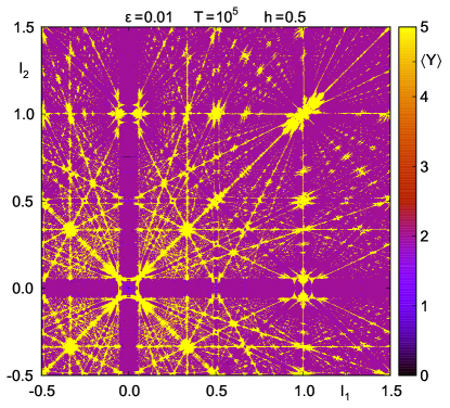
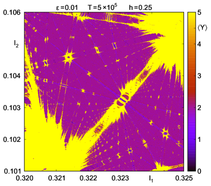
Figure 1: MEGNO dynamical maps of the model Hamiltonian (Eq. 1) in the actions $(I_{1},I_{2})$-plane, corresponding to the fundamental frequencies of the unperturbed model. Panels are for $\epsilon=0.01$. The left panel shows the quasi-global view of the phase space, with a close-up on the right. Solutions are colour-coded: stable solutions with the MEGNO $\sim 2$, unstable (chaotic) with the MEGNO cut-off at 5, and stable periodic orbits are marked with the MEGNO $\sim 0$. Original, raw resolution of the maps is $2048\times 2048$ points. The step-size $h$ of the symplectic SABA₃ integrator and total integration time are labeled.

3 Hamiltonian model of the Arnold Web

We illustrate programming concepts behind the Mechanic environment with the dynamical system derived by Froeschlé et al. (2000). The system is written in Hamiltonian form of

$${\cal H}={\cal H}_{0}(I_{1},I_{2},I_{3})+\epsilon V(\phi_{1},\phi_{2},\phi_{3}),$$ (1)

where the Hamiltonian terms are

$${\cal H}_{0} = \frac{1}{2}I_{1}^{2}+\frac{1}{2}I_{2}^{2}+I_{3},$$ (2)

$${\cal V} = \frac{1}{\cos\phi_{1}+\cos\phi_{2}+\cos\phi_{3}+4}.$$ (3)

Actions $I_{1},I_{2},I_{3}\in{\mathbb{R}}$ and angles $\phi_{1},\phi_{2},\phi_{3}\in{\mathbb{T}}$ are canonically conjugated variables, and $\epsilon$ is a parameter that measures the perturbation strength. Indeed, if $\epsilon=0$, the equations of motion of Hamiltonian ${\cal H}_{0}$ are trivially integrable. Because angles are cyclic in ${\cal H}_{0}$, actions $I_{1},I_{2},I_{3}$ are constant; then the angles are linear functions of time $\phi_{i}=f_{i}t+\phi_{i}(0)$, where

$$f_{i}=\frac{\partial{\cal H}}{\partial I_{i}}\equiv\frac{\partial{\cal H}_{0}}{\partial I_{i}},\quad i=1,2,3.$$

The motions generated by the integrable Hamiltonian are confined to invariant tori composed of quasi-periodic solutions having the fundamental frequencies $f_{1}=I_{1}$, $f_{2}=I_{2}$, $f_{3}=1$. With the perturbation term $\epsilon\neq 0$, the full dynamics are non-integrable. According with the Kolmogorov-Arnold-Moser theorem (KAM, Arnold, 1978), the quasi-periodic solutions persist in some volume of the phase space, provided that certain non-degeneracy conditions are fulfilled and the unperturbed tori are sufficiently non-resonant:

$$k_{1}f_{1}+k_{2}f_{2}+k_{3}f_{3}\neq 0,\quad k_{1},k_{2},k_{3}\in{\mathbb{Z}}.$$

The KAM theorem does not apply in a neighborhood of the resonances, which are represented as lines, up to the distance of the order of $\sqrt{\epsilon}\exp(-|\,{{\bf k}}\,|)$, where $|\,{{\bf k}}\,|$ is the order of the resonance. In that zone, called the Arnold web, the dynamics are extremely complex.

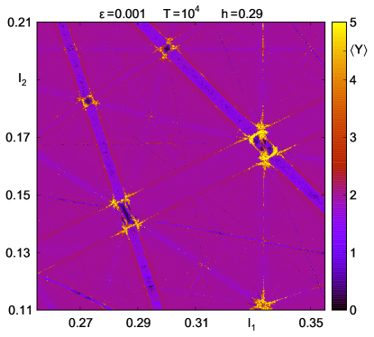
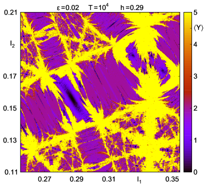
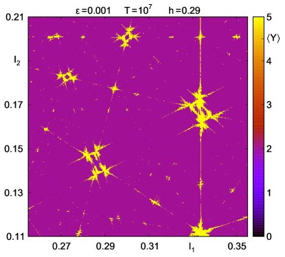
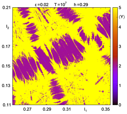
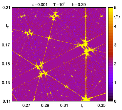
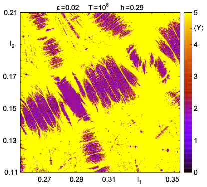
Figure 2: The Arnold diffusion shown with the MEGNO time-snapshots in a close-up region of the model Hamiltonian (Eq. 1) near the resonant line $I_{1}=2I_{2}$. Left panels are for $\epsilon=0.001$, which corresponds to the stable Nekhoroshev regime and the right for $\epsilon=0.02$, corresponding to the transition region between Nekhoroshev and Chirikov regimes (Lega et al., 2003). The stepsize of the symplectic SABA₃ and the total integration time are labeled. The raw resolution of the maps is $512\times 512$ points.

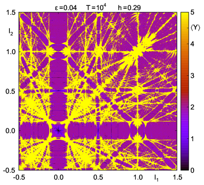
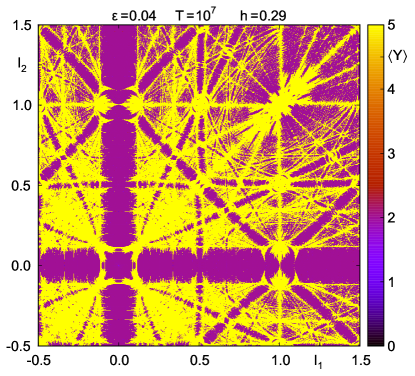
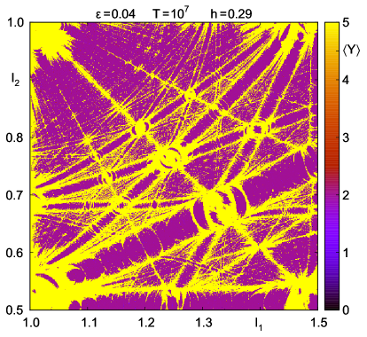
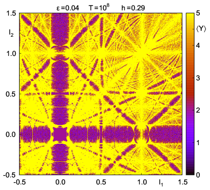
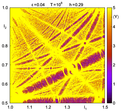
Figure 3: The evolution of the model Hamiltionian (Eq. 1) shown with the MEGNO time-snapshots. All panels are for $\epsilon=0.04$. The left panels show the global view in the actions $(I_{1},I_{2})$-plane. The close-up near the resonant line $I_{1}=2I_{2}$ is shown on the right. The stepsize of the symplectic SABA₃ and the total integration time are labeled. The raw resolution of the global maps is $1024\times 1024$ points, and the close-ups $512\times 512$ points.

Following Froeschlé et al. (2000), we visualize the structure of the Arnold web through applying a concept of dynamical maps. The Arnold web can be represented in two-dimensional actions plane, e.g., $(I_{1},I_{2})$, which correspond to fundamental frequencies of the unperturbed system (Froeschlé et al., 2000). To detect the regular and chaotic motions, which are expected in a non-integrable Hamiltonian system, we apply the fast indicator MEGNO (Cincotta and Simó, 2000). Recently, Mestre et al. (2011) showed analytically that this numerical tool brings essentially the same information as the Fast Lyapunov Indicator used by Froeschlé et al. (2000). They computed dynamical maps of the Arnold web for a few representative values of $\epsilon=0.001$, $\epsilon=0.01$ and $\epsilon=0.04$, with the resolution of $500\times 500$ pixels.

With the help of Mechanic, we attempt to illustrate the Arnold web in much larger resolutions revealing very fine details of the phase space. They appear due to resonances of large orders. It is only a matter of long enough integration time to detect all resonances, but much longer motion times than $10^{3}$ characteristic periods ($\equiv 1$) in the original paper are required. The general-purpose integrators, like the Runge-Kutta or Bulirsh-Stoer-Gragg schemes are not accurate nor efficient enough for that purpose. These methods introduce systematic drift of the energy (or other integrals). To avoid such errors, and to solve the variational equations required to compute the MEGNO indicator, we applied the symplectic tangent map algorithm introduced by Mikkola and Innanen (1999). In the past, we used this scheme for an efficient and precision computations of MEGNO for multiple planetary systems (Goździewski et al., 2003, 2005, 2008a).

The model Hamiltonian is particularly simple to illustrate the symplectic algorithm. It relies on concatenating maps $\Phi_{1,h}({{\bf I}},{{\bf\phi}})$ and $\Phi_{2,h}({{\bf I}},{{\bf\phi}})$ that solve the equations of motion derived from the unperturbed part ${\cal H}_{0}$, and the perturbation alone, on the time interval $[t_{0},t_{0}+h]$. The solutions may be constructed if both Hamiltonian terms admit analytical solutions. This is the case. For the unperturbed term we have

$$\frac{d}{dt}{{{\bf\phi}}}=\frac{\partial{\cal H}_{0}}{\partial{{\bf I}}},\quad\frac{d}{dt}{{{\bf I}}}=-\frac{\partial{\cal H}_{0}}{\partial{{\bf\phi}}}.$$

Then the “drift” map $\Phi_{1,h}({{\bf I}},{{\bf\phi}})$ map is the following:

$${{{\bf\phi}}}={{\bf\omega}}h+{{{\bf\phi}}}_{0},\quad{{{\bf I}}}={{{\bf I}}}_{0},$$

where ${{\bf f}}=(I_{1},I_{2},1)$. The equations of motion generated by the perturbation Hamiltonian $H_{1}\equiv\epsilon V({{\bf\phi}})$ alone are also soluble, hence we obtain the “kick” map $\Phi_{2,h}({{\bf I}},{{\bf\phi}})$:

$${{{\bf\phi}}}={{{\bf\phi}}}_{0},\quad{{{\bf I}}}={{\bf\Omega}}h+{{{\bf I}}}_{0},\qquad{{\bf\Omega}}=-\epsilon\frac{\partial{\cal V}({{\bf\phi)}}}{\partial{{\bf\phi}}}.$$

A classic leap-frog concatenation of these maps

$$\Phi\equiv\Phi_{1,h/2}\odot\Phi_{2,h}\odot\Phi_{1,h/2},$$

provides a numerical integrator of the second order with local error ${\cal O}(\epsilon h^{2})$. However, because we deal with a small perturbation parameter, much better performance and accuracy can be obtained by applying symplectic schemes invented by Laskar and Robutel (2001). The $n$-th order integrator, e.g., SABA_n, have the truncation error ${\cal O}(\epsilon^{2}h^{2}+\epsilon h^{n})$. For small $\epsilon$ it behaves like a higher-order scheme without introducing negative sub-steps. In our computations, we used the SABA₃ scheme. We found that it provides an optimal performance, CPU-overhead vs. the relative error of the energy.

To compute the MEGNO, we must solve the variational equations to the equations of motion. We use the algorithm described in (Goździewski et al., 2008a). The tangent map approach (Mikkola and Innanen, 1999) requires to differentiate the “drift” and “kick” maps. This step is straightforward. The variations are propagated within the same symplectic scheme, as the equations of motion. Having the variational vector ${{\bf\delta}}$ computed at discrete times, we find temporal $y$ and mean $Y$ values of the MEGNO indicator at the $j$-th integrator step ($j=1,2,\ldots$) in the form of (Cincotta et al., 2003; Goździewski et al., 2008a):

$$Y(j) = \frac{(j-1)Y(j-1)+y(j)}{j},$$

$$y(j) = \frac{j-1}{j}y(j-1)+2\ln\left(\frac{\delta_{j}}{\delta_{j-1}}\right),$$

with initial conditions $y(0)=0$, $Y(0)=0$, $\delta=|\,{{\bf\delta}}\,|$. Following Cincotta et al. (2003), the MEGNO map obtained in this way tends asymptotically to

$$Y(j)=ahj+b,$$

where $a=0,b\sim 2$ for quasi-periodic orbits, $a=b=0$ for stable, periodic orbit, and $a=(1/2)\sigma,b=0$ for chaotic orbit with the maximal Lyapunov exponent $\sigma$.

Thanks to the linearity of the tangent MEGNO map, the variational vector can be normalized, if its value grows too large for chaotic orbits. In practice, we stop the integration if MEGNO reaches a given limit ($Y=5$ in this particular case).

4 The results

We conducted simulations of MEGNO maps in parallel using the Mechanic framework up to 2048 CPUs installed at the Reef, Cane and Chimera clusters (Poznań Supercomputing Centre, PCSS). Simulations were performed using the master–worker communication mode. The resolution of the maps varied between $512\times 512$ up to $2048\times 2048$ points. The actions $(I_{1},I_{2})$-plane has been regularly spaced according to the run-time configuration and the task coordinates on the task assignment grid. For each initial condition, different initial variational vector has been choosen. The other initial conditions were: $I_{3}(0)=1$ and $\phi_{1}(0)=\phi_{2}(0)=\phi_{3}(0)=0$. Technical details of the module implementation are given in the Appendix.

The results for model Hamiltonian (Eq. 1) are illustrated on the Fig. 1. The left panel shows the quasi-global view of the $(I_{1},I_{2})$-plane for the $\epsilon=0.01$ and $T=10^{5}$. The resonances appear as straight lines. The yellow (light-gray) colour encodes chaotic orbits, and the purple (dark-gray) colour denotes $\langle Y\rangle\sim 2$ of stable, quasi-periodic solutions. According to Froeschlé et al. (2000), the dynamics is governed by the Nekhoroshev regime, when the most of invariant tori of the perturbed system exist. However, as shown in Lega et al. (2003), diffusing orbits exists along the resonances. This leads to significant drifts in the actions space (Guzzo et al., 2004; Froeschlé et al., 2005, 2006). This phenomenon, called the Arnold diffusion is closely related to the stability of the system, and was suggested by Arnold (1964) in the three-body problem.

To illustrate the Arnold diffusion, we computed MEGNO time-snapshots over the time-span $T=10^{4}-10^{8}$. The slow diffusion in the stable Nekhoroshev regime ($\epsilon=0.001$) is shown on the left panels of the Fig. 2. Most of solutions remains quasi-stable after $T=10^{8}$. However, for large $\epsilon$, the diffusion is not forced along the resonances. Instead, the resonances overlap and the diffusing orbits may wander between different resonances (Lega et al., 2003). This transition region for $\epsilon=0.02$ is illustrated on the right panels of the Fig. 2. At the critical value, the region of diffusing orbits replaces the region of invariant tori, and the dynamics is governed by the Chirikov regime. As estimated by Froeschlé et al. (2000), the critical $\epsilon$ for the Hamiltonian (Eq. 1) is $0.04$ (Fig. 3). Most of the phase space becomes chaotic after $T=10^{8}$.

Computations were performed with different step-sizes, $h=0.01$ up to $h=0.5(\sqrt{5}-1)\sim 0.29$, and $h=0.5$. We found that even such large integration steps do not introduce artificial (numerical) resonances. As an example, we selected a very small region close to the centre of the global map (the left panel in Fig. 1), and we computed MEGNO maps with different step sizes over $T=10^{6}$ using SABA₃ and SABA₄ integrators. The results for $h\sim 0.06$ and $h=0.5$ are shown on the Fig. 4. Both the close-ups reveal very fine details of the phase space, and cannot be distinguished each from the other. This test assured us, that relatively large step-sizes of the order of $h\sim 10^{-1}$ are still safe, and the results are reliable. The relative energy error was preserved up to $10^{-8}-10^{-9}$ over the total integration times up to $T\sim 10^{8}$.

Depending on the characteristic period $T$, the resolution of the maps and the number of CPU cores involved, the total simulation time of a single map took up to 72 hours.

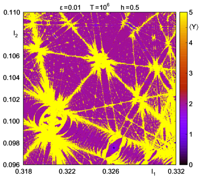
Figure 4: Close-ups of the MEGNO dynamical maps for $\epsilon=0.01$ and $T=10^{6}$. The left panel shows the result computed with the step size $\sim 0.061$ and the right panel for the step size $0.5$ of the SABA₃ integrator.

5 Summary

We present the Mechanic code, an open-source MPI/HDF5 code framework. It is designed to become a helper tool for conducting massive numerical computations that rely on testing huge volume of inital conditions, such as studies of long-term orbital evolution and stability of planetary systems with Monte Carlo methods or dynamical maps, as well as modelling observations with evolutionary algorithms. Based on the core–module approach, the framework reduces the development effort of a scientific application, by providing skeleton code for common technical operations, such as data and configuration management, as well as task distribution on the parallel computing environments. Within the framework, the user’s application may be reduced to a module form containing the numerical algorithm with the required setup and storage specifications. Unlike the existing task management software, such as HTCondor or Workqueue, our framework is based on the unified data storage approach, that is built on top of the HDF5 library. This reduces the post-processing effort and makes it possible to use results of the simulation in numerous external applications written in different programming languages, such as Python. The framework supports multidimensional datasets of all basic datatypes with attributes. The communication and storage layers are hidden to the end user, so that, no knowledge on the parallel programming is required to use the framework.

The Mechanic has been already extensively tested in the dynamical studies of the Kepler-11 (Migaszewski et al., 2012) and $\nu$Oct systems (Goździewski et al., 2013). They validated the framework as a helper tool for astronomical research. The numerical computations have been conducted up to 2048 CPUs on the Reef, Cane and the SGI UV Chimera supercomputer located at the Poznań Supercomputing Centre. In this paper, we have shown the usage of the framework with the simple dynamical map algorithm applied to the Hamiltonian model of the Arnold Web. The source code of the framework is shipped with template modules, that show every aspect of the API. This includes using predefined initial conditions list for the input, programmatic generation of initial conditions as well as simple genetic algorithm implementation. The code is BSD-licensed and available at the project page.

Appendix A Detailed code listings for the Arnold Web module

A Mechanic module is a C-interoperable code compiled to a shared library. It consists of a set of API functions that correspond to the well-known user’s application flow. The Init() hook (Listing 3) is used for module-related initializations, including the number of memory buffers passed between the master and workers. The setup stage is performed via the information specified in the Setup() hook (Listing 4). All configuration options are available during the run-time, both in the configuration file and the command-line.

The file and memory management is performed according to the specification given in the Storage() hook (Listing 5). For the purpose of the Arnold Web example, we define two data buffers. The result buffer is dedicated to storing the master result. Each worker node allocates the memory according to the specified dimensionality and datatype of the buffer. In this particular case, the result buffer is of size $1\times 1\times 10\times 2$, and contains the MEGNO value and relative energy error over a maximum of 10 time-snapshots. The master node assembles the partial results received from workers into a single, four-dimensional dataset of texture type, with the respect to the task location on the grid. For example, in a $2048\times 2048$ points simulation we will obtain the dataset of size $2048\times 2048\times 10\times 2$, with third dimension (slice) representing time-snapshots and the last dimension containing the actual result. The second buffer, state, contains the temporary integration data and is removed after successful completion of all tasks. Otherwise, it may be used to restart the simulation from the last stored checkpoint.

The actual computations are performed within the TaskPrepare() and TaskProcess() hooks (Listings 6 and 7). We change the initial condition according to the run-time configuration and the task coordinates on the task assignment grid. This occurs only on the first time-snapshot indicated by the task checkpoint id cid = 0. The checkpoint id increments while the TaskProcess() returns TASK_CHECKPOINT. At each task checkpoint we change the integration time to obtain snapshots with the power-based intervals, starting with the minimum characteristic period required by the MEGNO, $T=10^{4}$. The simulation is continued with the initial condition that is read from the state buffer. The result is returned to the master. After the last snapshot has been completed, the task is finalized, and the worker node takes the next one, if available.

Listing 3: The module initialization. The banks_per_task setting of the Init() hook specifies the number of memory buffers available for the each task.

⬇

#include "mechanic.h"

#include <math.h>

#define MAX_SNAPSHOTS 10

int saba3(double *state, double step,

double tstart, double tend, double eps,

double *megno, double *err);

/* Implements Init() */

int Init(init *i) {

i->banks_per_task = 2;

return SUCCESS;

}

Listing 4: The Setup() hook. Each configuration option is defined within the module space. All fields are mandatory. The name and shortName define the long and short option name respectively. The default value value is used, when the option has not been overridden in the configuration file nor the command-line. Supported types: C_INT, C_LONG, C_FLOAT, C_DOUBLE, C_VAL (boolean) and C_STRING.

⬇

/* Implements Setup() */

int Setup(setup *s) {

s->options[0] = (options) {

.space = "aweb", .name = "step", .shortName = ’\0’,

.value = ’0.5’, .type = C_DOUBLE,

.description = "Integrator step size"

};

s->options[1] = (options) {

.space = "aweb", .name = "eps", .shortName = ’\0’,

.value = ’0.01’, .type = C_DOUBLE,

.description = "The perturbation parameter"

};

s->options[2] = (options) OPTIONS_END;

return SUCCESS;

}

Listing 5: The Storage() hook. The data buffers are defined per task pool p. They are available during the simulation through the task t object. The HDF5 dataset path is configured via the name field. The maximum dimensionality of a memory buffer (and the corresponding dataset) is 32 (defined via H5S_MAX_RANK).

⬇

/* Implements Storage() */

int Storage(pool *p) {

// Path: /Pools/pool-ID/Tasks/result

p->task->storage[0].layout = (schema) {

.name = "result",

.rank = 4,

.dims[0] = 1, //y-dim

.dims[1] = 1, //x-dim

.dims[2] = MAX_SNAPSHOTS,

.dims[3] = 2,

.use_hdf = HDF_NORMAL_STORAGE,

.storage_type = STORAGE_TEXTURE,

.datatype = H5T_NATIVE_DOUBLE

};

// Temporary storage for the state variables

p->task->storage[1].layout = (schema) {

.name = "state",

.rank = 2,

.dims[0] = 1,

.dims[1] = 24,

.use_hdf = HDF_TEMP_STORAGE,

.storage_type = STORAGE_LIST,

.datatype = H5T_NATIVE_DOUBLE

};

return SUCCESS;

}

Listing 6: The TaskPrepare() hook. The initial condition is prepared according to the current run-time configuration, which is provided in the pool p object. The configuration is accessed with the MReadOption macro. It takes the current pool object and the option name as arguments and reads the option value to the specified local variable. The state and result buffers are prepared at the beginning of the simulation (the task checkpoint id, cid, is 0). The initial data from local arrays is written to the task memory buffers with the MWriteData macro. It is available then in other API hooks.

⬇

/* Implements TaskPrepare() */

int TaskPrepare(pool *p, task *t) {

double state[24];

double r[1][1][MAX_SNAPSHOTS][2];

double xmin, xmax, ymin, ymax;

double stepx, stepy;

int xres, yres, i;

if (t->cid == 0) {

MReadOption(p, "xmin", &xmin);

MReadOption(p, "xmax", &xmax);

MReadOption(p, "ymin", &ymin);

MReadOption(p, "ymax", &ymax);

MReadOption(p, "xres", &xres);

MReadOption(p, "yres", &yres);

stepx = (xmax-xmin)/((double)xres);

stepy = (ymax-ymin)/((double)yres);

// Initial data

for (i = 0; i < 24; i++)

state[i] = 0.0;

state[3] = xmin + t->location[1]*stepx;

state[4] = ymin + t->location[0]*stepy;

state[5] = 1.0;

// Randomize the tangent vector

for (i = 6; i < 12; i++)

state[i] = rand()/(RAND_MAX+1.0);

MWriteData(t, "state", &state[0]);

// Prepare the result buffer

for (i = 0; i < MAX_SNAPSHOTS; i++) {

r[0][0][i][0] = 0.0;

r[0][0][i][1] = 0.0;

}

MWriteData(t, "result", &r[0][0][0][0]);

}

return SUCCESS;

}

Listing 7: The TaskProcess() hook. Before the computations, we read the initial condition from the state buffer to the local buffer with the MReadData macro. The data is passed then to the numerical integrator, among with the current time interval. After the computations, the result is written to the buffer, and returned to the master node. If the TaskProcess() hook returns TASK_CHECKPOINT, the worker continues evaluation of the current task with the new time interval based on the task checkpoint id. The TASK_FINALIZE indicates successfull evaluation of the task and the worker node takes the next one, if available. In case of any error, the hook may return error code, as specified in the API documentation.

⬇

/* Implements TaskProcess() */

int TaskProcess(pool *p, task *t) {

double state[24];

double result[1][1][MAX_SNAPSHOTS][2];

double tstart = 0.0, tend = 0.0, step = 0.0;

double megno = 0.0, err = 0.0, eps = 0.0;

int snapshots, status = SUCCESS;

MReadOption(p, "task-checkpoints", &snapshots);

MReadOption(p, "eps", &eps);

MReadOption(p, "step", &step);

// power-based time intervals

if (t->cid == 0) tstart = 0.0;

else tstart = pow(10, t->cid + 4);

tend = pow(10, t->cid + 5);

step = step*(pow(5,0.5)-1)/2.0;

MReadData(t, "state", &state[0]);

if (t->cid > 0) {

MReadData(t, "result", &result[0][0][0][0]);

}

// Numerical integration goes here

status = saba3(state, step, tstart, tend,

eps, &megno, &err);

if (status < 0) return MODULE_ERR_OTHER;

// Assign the master result

result[0][0][t->cid][0] = megno;

result[0][0][t->cid][1] = err;

MWriteData(t, "result", &result[0][0][0][0]);

MWriteData(t, "state", &state[0]);

if (t->cid + 1 == snapshots) return TASK_FINALIZE;

return TASK_CHECKPOINT;

}

Listing 8: The module compilation. The code of the module must be compiled to a shared library with libmechanic_module_ prefix. The module should be linked with the mechanic library and available in the user’s LD_LIBRARY_PATH.

⬇

mpicc -fPIC -Dpic -shared aweb.c \

-o libmechanic_module_aweb.so \

-lmechanic -lm -lhdf5

Listing 9: Using the module. The Mechanic should be invoked with mpiexec or mpirun scripts. The user’s module is specified with the -p (--module) option. In the example below, the aweb module is invoked on the 2048 CPUs in the default, master–worker mode. The total resolution of the simulation is $2048\times 2048$ points. The result of the simulation will be stored in the master file arnold-web-master-00.h5. The framework ships with the predefined options helpful for conducting computations, such as run-time resolution or number of checkpoints. The full list of options is given with the --help switch.

⬇

mpirun -np 2048 mechanic -p aweb \

--xres=2048 --yres=2048 \

--xmin=-0.5 --xmax=1.5 \

--ymin=-0.5 --ymax=1.5 \

--step=0.5 --eps=0.04 \

--task-checkpoints=5 \

--name=arnold-web

References

- Arnold (1964) Arnold, V. I., Dec. 1964. Instability of dynamical systems with several degrees of freedom. Doklady Akad. Nauk SSSR (in Russian) 5, 581–585.
- Arnold (1978) Arnold, V. I., 1978. Mathematical methods of classical mechanics.
- Barrio et al. (2009) Barrio, R., Borczyk, W., Breiter, S., May 2009. Spurious structures in chaos indicators maps. Chaos Solitons and Fractals 40, 1697–1714.
- Cincotta (2002) Cincotta, P. M., Jan. 2002. Arnold diffusion: an overview through dynamical astronomy. New Astronomy 46, 13–39.
- Cincotta et al. (2003) Cincotta, P. M., Giordano, C. M., Simó, C., Aug. 2003. Phase space structure of multi-dimensional systems by means of the mean exponential growth factor of nearby orbits. Physica D Nonlinear Phenomena 182, 151–178.
- Cincotta and Simó (2000) Cincotta, P. M., Simó, C., Dec. 2000. Simple tools to study global dynamics in non-axisymmetric galactic potentials - I. A&A 147, 205–228.
-
Fields (1993)
Fields, S., 1993. Hunting For Wasted Computing Power. New Software for
Computing Networks Puts Idle PC’s to Work.
URL http://www.cs.wisc.edu/condor/doc/WiscIdea.html - Froeschlé et al. (2000) Froeschlé, C., Guzzo, M., Lega, E., Sep. 2000. Graphical Evolution of the Arnold Web: From Order to Chaos. Science 289, 2108–2110.
- Froeschlé et al. (2005) Froeschlé, C., Guzzo, M., Lega, E., Apr. 2005. Local And Global Diffusion Along Resonant Lines in Discrete Quasi-integrable Dynamical Systems. Celestial Mechanics and Dynamical Astronomy 92, 243–255.
- Froeschlé et al. (1997) Froeschlé, C., Lega, E., Gonczi, R., Jan. 1997. Fast Lyapunov Indicators. Application to Asteroidal Motion. Celestial Mechanics and Dynamical Astronomy 67, 41–62.
- Froeschlé et al. (2006) Froeschlé, C., Lega, E., Guzzo, M., May 2006. Analysis of the Chaotic Behaviour of Orbits Diffusing along the Arnold Web. Celestial Mechanics and Dynamical Astronomy 95, 141–153.
- Goździewski et al. (2008a) Goździewski, K., Breiter, S., Borczyk, W., Jan. 2008a. The long-term stability of extrasolar system HD37124. Numerical study of resonance effects. MNRAS 383, 989–999.
- Goździewski et al. (2003) Goździewski, K., Konacki, M., Maciejewski, A. J., Sep. 2003. Where is the Second Planet in the HD 160691 Planetary System? ApJ 594, 1019–1032.
- Goździewski et al. (2005) Goździewski, K., Konacki, M., Wolszczan, A., Feb. 2005. Long-Term Stability and Dynamical Environment of the PSR 1257+12 Planetary System. ApJ 619, 1084–1097.
- Goździewski and Migaszewski (2009) Goździewski, K., Migaszewski, C., Jul. 2009. Is the HR8799 extrasolar system destined for planetary scattering? MNRAS 397, L16–L20.
- Goździewski et al. (2008b) Goździewski, K., Migaszewski, C., Musieliński, A., May 2008b. Stability constraints in modeling of multi-planet extrasolar systems. In: Sun, Y.-S., Ferraz-Mello, S., Zhou, J.-L. (Eds.), IAU Symposium. Vol. 249 of IAU Symposium. pp. 447–460.
- Goździewski et al. (2013) Goździewski, K., Słonina, M., Migaszewski, C., Rozenkiewicz, A., Mar. 2013. Testing a hypothesis of the Octantis planetary system. MNRAS 430, 533–545.
- Guzzo (2005) Guzzo, M., Mar. 2005. The web of three-planet resonances in the outer Solar System. Icarus 174, 273–284.
- Guzzo (2006) Guzzo, M., Apr. 2006. The web of three-planet resonances in the outer Solar System. II. A source of orbital instability for Uranus and Neptune. Icarus 181, 475–485.
- Guzzo et al. (2004) Guzzo, M., Lega, E., Froeschle’, C., Jul. 2004. First numerical evidence of global Arnold diffusion in quasi–integrable systems. eprint arXiv:nlin/0407059.
- Holman and Wiegert (1999) Holman, M. J., Wiegert, P. A., Jan. 1999. Long-Term Stability of Planets in Binary Systems. AJ 117, 621–628.
- Laskar (1993) Laskar, J., May 1993. Frequency analysis of a dynamical system. Celestial Mechanics and Dynamical Astronomy 56, 191–196.
- Laskar and Robutel (2001) Laskar, J., Robutel, P., Jul. 2001. High order symplectic integrators for perturbed Hamiltonian systems. Celestial Mechanics and Dynamical Astronomy 80, 39–62.
- Lega et al. (2003) Lega, E., Guzzo, M., Froeschlé, C., Aug. 2003. Detection of Arnold diffusion in Hamiltonian systems. Physica D Nonlinear Phenomena 182, 179–187.
- Mestre et al. (2011) Mestre, M. F., Cincotta, P. M., Giordano, C. M., Jun. 2011. Analytical relation between two chaos indicators: FLI and MEGNO. MNRAS 414, L100–L103.
- Michtchenko and Ferraz-Mello (2001) Michtchenko, T. A., Ferraz-Mello, S., Jul. 2001. Resonant Structure of the Outer Solar System in the Neighborhood of the Planets. AJ 122, 474–481.
- Migaszewski et al. (2012) Migaszewski, C., Słonina, M., Goździewski, K., Nov. 2012. A dynamical analysis of the Kepler-11 planetary system. MNRAS 427, 770–789.
- Mikkola and Innanen (1999) Mikkola, S., Innanen, K., May 1999. Symplectic Tangent Map for Planetary Motions. Celestial Mechanics and Dynamical Astronomy 74, 59–67.
- Pacheco (1996) Pacheco, P., 1996. Parallel Programming with MPI. Morgan Kaufmann.
- Robutel and Laskar (2001) Robutel, P., Laskar, J., Jul. 2001. Frequency Map and Global Dynamics in the Solar System I. Short Period Dynamics of Massless Particles. Icarus 152, 4–28.
- Sidlichovský and Nesvorný (1996) Sidlichovský, M., Nesvorný, D., Mar. 1996. Frequency modified Fourier transform and its applications to asteroids. Celestial Mechanics and Dynamical Astronomy 65, 137–148.
-
The HDF5 Group (2012)
The HDF5 Group, 2012. Hierarchical data format, http://www.hdfgroup.org.
URL http://www.hdfgroup.org/ - Yu et al. (2010) Yu, L., Moretti, C., Thrasher, A., Emrich, S., Judd, K., Thain, D., 2010. Harnessing parallelism in multicore clusters with All-Pairs, Wavefront, and Makeflow abstractions. Cluster Computing 13, 243–256.