Rheological aspects Emulsions and foams Plasticity and superplasticity

Rheology of athermal amorphous solids: Revisiting simplified scenarios and the concept of mechanical noise temperature.

Abstract

We study the rheology of amorphous solids in the limit of negligible thermal fluctuations. General arguments indicate that the shear-rate dependence of the stress results from an interplay between the time scales of the macroscopic drive and the (cascades of) local particle rearrangements. Such rearrangements are known to induce a redistribution of the elastic stress in the system. Although mechanical noise, i.e., the local stress fluctuations arising from this redistribution, is widely believed to activate new particle rearrangements, we provide evidence that casts severe doubt on the analogy with thermal fluctuations: mechanical and thermal fluctuations lead to asymptotically different statistics for barrier crossing. These ideas are illustrated and supported by a simple elasto-plastic model whose ingredients are directly connected with the physical processes relevant for the flow.

A disordered assembly of interacting particles, packed densely enough for the system to be able to bear stress, provides a realistic image of an amorphous solid - a heap of sand, a foam, an emulsion, a colloidal glass, a molecular glass, etc., depending on whether the particles are grains, air bubbles, drops, colloids or molecules. If the particles are not, or are hardly, affected by thermal fluctuations, the material is said to be athermal. External drive is then required to activate the dynamics of the system. When the material is shear driven, the flow curve, that is, the relation between the applied shear rate $\dot{\gamma}$ and the macroscopic shear stress $\Sigma$, is often satisfactorily described by a Herschel-Bulkley equation, $\Sigma=\Sigma_{0}+A\dot{\gamma}^{n}$, with an exponent $n$ usually close to, or slightly lower than, 0.5 [1, 2, 3, 4, 5, 6]. An unsettled question, however, regards the connection of this dependence on the driving velocity with the widely accepted picture for the spatial organisation of the flow of disordered solids. The slow flow scenario for these materials [7, 8, 9, 10] revolves around localised particle rearrangements (plastic events) bursting in an essentially elastically deforming matrix. The “mechanical noise” generated by these rearrangements, i.e., the fluctuating stress and strain fields that they induce in the surrounding medium, may then spark off new rearrangements, in an avalanche-like process.

In the first part of this Letter, we clarify the physical processes leading to the shear-rate dependence of the stress in this scenario. For all their success in capturing various facets of the rheology [11, 12, 13, 14, 15, 16, 17], simple coarse-grained models in the literature generally fail to reflect these key processes consistently for athermal materials. We remedy this deficiency by proposing a variant of such models and show that it satisfactorily reproduces the flow curve. In the second part of the Letter, we contemplate whether the description can be simplified by interpreting the fluctuating mechanical noise, which is explicitly computed in our model, as an effective activation temperature, following a popular approach in another line of modelling[12]. We conclude on more general grounds that the analogy between mechanical noise and an activation temperature is flawed.

Consider a dense packing of particles confined between parallel walls and subject to a (macroscopically) constant shear rate $\dot{\gamma}$, imposed through successive infinitesimal displacements of one of the walls. We start our discussion with an enumeration of the time scales that subsist in the limit of vanishing shear rate. To do so, we focus on a “mesoscopic” region of the typical size of a plastic event. First in line comes the time scale for thermally-activated structural relaxation, $\tau_{T}$ [18], which diverges in the athermal limit. Secondly, the response of the region of interest to a small displacement of the wall can take a finite time, $\tau_{pl}$. This time will then essentially combine the duration of a local rearrangement, i.e., the time needed to dissipate the elastic energy that was stored locally [19, 18], with the delay for shear signal transmission within one avalanche [20]. $\tau_{T}$ and $\tau_{pl}$ are the only potentially relevant time scales when $\dot{\gamma}\rightarrow 0$. Within a potential energy landscape (PEL) description, they are associated with thermally-activated hops between energy (meta)basins, and descents towards the local minimum, respectively.

The application of a finite shear rate introduces a new time scale, $\dot{\gamma}^{-1}\gamma_{y}$, which is the duration of the elastic loading phase prior to yield. In the PEL viewpoint, this is the “refresh rate” of the PEL topology, owing to changes in the boundary conditions.

As stated in [9], quasistatic simulations, which perform an energy minimisation after each strain increment, rely on the following separation of the material and driving timescales:

$$\tau_{pl}\lll\dot{\gamma}^{-1}\lll\tau_{T}.$$ (1)

As long as eq. 1 holds, the system will follow the very same trajectory in phase space as a function of the strain $\gamma\equiv\dot{\gamma}t$, regardless of the shear rate, thereby yielding a constant elastic stress $\sigma_{el}$. One should now recall that, for a solid-like material at low shear rate, the elastic stress dominates the total stress $\Sigma$ to such an extent that the dissipative contribution to the stress is often discarded in computer simulations, $\Sigma\approx\sigma_{el}$ [21]. Accordingly, the only way to recover a non constant flow curve $\Sigma\left(\dot{\gamma}\right)$ involves a breakdown of the timescale separation, eq. 1, and thus, for athermal materials, an interplay between the drive and the (cascades of) localised rearrangements. In granular media or suspensions of hard particles, this is quantified by a dimensionless inertial or viscous number [22]. More generally, the descent towards the energy minimum of the system is disrupted by the external drive. The impossibility for the system to fully relax between strain increments (see fig. 1(right) in ref. [23]) is reflected, for instance, by the variations of the mean particle overlaps with the shear rate. Near the jamming transition, these variations are correlated to the flow curve [24]. Deeper in the solid phase, where the simple flow scenario outlined above has proved its consistency, strain accumulation during the propagation of shear waves sets a shear-rate dependent limit on the spatial extent of the avalanches observed in athermal particle-based simulations [3].

Surprisingly, when surveying existing coarse-grained models, one realizes that they generally do not attempt to describe the disruption of rearrangements by the drive. For instance, in Hébraud-Lequeux’s model [25], or in the Kinetic Elastoplastic theory [14], as well as in Picard’s model [13, 26], the increase of the stress as $\dot{\gamma}$ increases derives from the hypothesised conservation of an elastic behaviour on a given site for a constant time (on average) after the stress threshold has been reached locally, which appears unphysical.

Therefore, we present a variant of these models which reflects the physical processes at play. A 2D system is discretised into linear elastic blocks of uniform shear modulus $\mu$ and of the size of a rearranging region. To condense notations, the deviatoric stress borne by each block ${(i,j)}$ is written $\boldsymbol{\sigma}(i,j)=[\sigma_{xx}(i,j),\,\sigma_{xy}(i,j)]^{\top}$. The onset of a plastic event on a given block is determined by a von Mises yield criterion: as soon as the maximal shear stress $\left\|\boldsymbol{\sigma}(i,j)\right\|\equiv\sqrt{\sigma_{xx}^{2}(i,j)+\sigma_{xy}^{2}(i,j)}$ grows larger than the local yield stress, defined below, the block yields. One then has a stress-laden fluid-like inclusion in an elastic medium. An unconstrained inclusion would deform at a rate $\boldsymbol{\dot{\epsilon}}^{pl}\equiv\boldsymbol{\sigma}(i,j)/2\eta_{\mathrm{eff}}$, with $\eta_{\mathrm{eff}}$ the effective viscosity of the inclusion, in the overdamped regime; a time scale $\tau\equiv\eta_{\mathrm{eff}}/\mu$ for local energy dissipation thus arises[19]. However, this deformation is limited by the embedding elastic medium, and part of the stress borne by the inclusion is gradually redistributed to the latter. The stress redistribution is described by an elastic propagator (matrix) $\mathcal{G}$, which was derived in ref. [19] for a pointwise inclusion in an incompressible, uniform, linear elastic medium, under the assumption of infinite shear wave velocity. As the pointwise limit of a 2D Eshelby inclusion problem [28], $\mathcal{G}$ also features an $r^{-2}$ decay in space and a four-fold angular symmetry, in accordance with experimental and numerical evidence [29, 30].

According to the above mechanism, the evolution of the local stress tensor is governed by,

$$\partial_{t}\boldsymbol{\sigma}(i,j)=\mu\boldsymbol{\dot{\gamma}}+2\mu\sum_{i^{\prime},j^{\prime}}\mathcal{G}_{i-i^{\prime},j-j^{\prime}}\boldsymbol{\dot{\epsilon}}^{pl}(i^{\prime},j^{\prime}),$$ (2)

where $\boldsymbol{\dot{\epsilon}}^{pl}(i^{\prime},j^{\prime})=\boldsymbol{\sigma}(i^{\prime},j^{\prime})/2\mu\tau$ if the block is plastic, 0 otherwise. The second term on the right hand side of eq. 2, describes the effect of plastic events, i.e., both the nonlocal stress redistribution and the local stress decay. The eigenvalues of the local component $\mathcal{G}_{0,0}$ are of order $-0.5$, so that the stress within a plastic element would decay to zero on a time scale $\tau$ in the absence of external loading or elastic recovery.

To fix the distribution of yield stresses $\sigma_{y}$, or, equivalently, of energy barriers $E_{y}\equiv\sigma_{y}^{2}/4\mu$, and the duration of a plastic event, we reason on the basis of a schematic vision of the PEL of a rearranging region. This landscape is composed of metabasins of exponentially distributed depths $E_{y}$, as suggested by some experimental results on colloidal glasses [31] and as in the Soft Glassy Rheology (SGR) model [12]. For practical reasons, we neglect small jumps between PEL basins and focus on the larger jumps between metabasins, which correspond to the irreversible jumps at low enough temperature [32, 33]; to this end, we simply introduce a lower cut-off $E_{y}^{min}=\nicefrac{{\mu\gamma_{c}^{2}}}{{4}}$ in the energy distribution, via a Heaviside function $\Theta$, viz.,

$$P\left(E_{y}\right)=\Theta\left(E_{y}-E_{y}^{min}\right)\lambda e^{\lambda\left(E_{y}^{min}-E_{y}\right)},$$ (3)

where $\lambda$ is chosen so that the average yield strain $\left\langle\gamma_{y}\right\rangle$ takes a realistic value, say, $10\%$ for emulsions [8]. In order to describe elastic recovery, we further assume that there is some typical distance (measured in terms of strain) between metabasin minima. This distance is related to the parameter $\gamma_{c}$ used to define $E_{y}^{min}$; for simplicity, it is set to exactly $\gamma_{c}$. A block will then remain plastic until the strain $\gamma_{c}$ has been cumulated during plasticity, that is, as long as $\int dt\left\|2\boldsymbol{\dot{\epsilon}}(i,j)\left(t\right)\right\|<\gamma_{c}$, where the local rate of deformation $\boldsymbol{\dot{\epsilon}}(i,j)$ is the sum of the plastic strain rate, $\boldsymbol{\dot{\epsilon}}^{pl}(i,j)$, and an elastic component, $\partial_{t}\boldsymbol{\sigma}(i,j)/2\mu$, which includes the reaction of the medium and the external loading (see eq. 2). Albeit somewhat arbitrary, this criterion for elastic recovery is physically plausible in a PEL perspective, and it provides a convenient way to implement the aforementioned disruption of plastic events by the drive. At the end of the plastic event, the local energy barrier is renewed. Apart from the time and stress units, $\tau$ and $\mu$, the only parameter left free in the model is the ratio $\gamma_{c}/\langle\gamma_{y}\rangle$, which we set to $0.7$. (Changing this value brings on but slight variations of the results).

The flow curve obtained from simulations of the model is plotted in fig. 1. Quite interestingly, at reasonably low shear rates $\dot{\gamma}<10^{-2}$, the curve is nicely fit by a Herschel-Bulkley equation with exponent $n=0.56$. It is noteworthy that the Herschel-Bulkley fit holds not only in the direct vicinity of the yield stress, as in other coarse-grained models [8, 14, 12], but over a reasonably large window of shear rates, in accordance with experimental observations [1, 2, 4]. At higher shear rates, for $\dot{\gamma}\tau>\left\langle\gamma_{y}\right\rangle$, one enters a regime dominated by the dissipative stress during plastic events, which was assumed linear in the strain rate here.

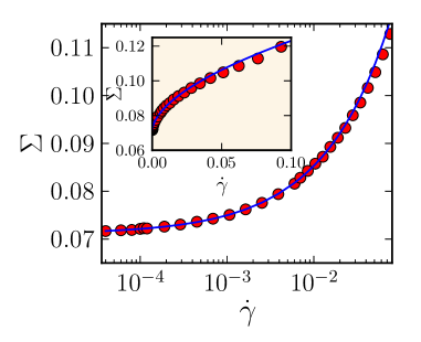
Figure 1: Macroscopic shear stress $\Sigma$ as a function of the applied shear rate $\dot{\gamma}$, for $\nicefrac{{\gamma_{c}}}{{\left\langle\gamma_{y}\right\rangle}}=0.7.$ The solid line is the fitting curve $\Sigma=0.071+0.19\dot{\gamma}^{0.56}$. (Inset) Same data, in linear-linear plot.

Note that the flow curve already rises at very low shear rates in our model. Around $\dot{\gamma}^{-1}\sim 10^{3}$ the life time of a plastic event (of order $\tau$) is two orders of magnitude shorter than $\gamma_{y}\dot{\gamma}^{-1}$, and a stress increase is already seen. This feature may be applicable to experimental systems such as foams, for which the flow curve rises even when the inverse strain rate is much longer than an elementary rearrangement of bubbles (“T1 event”).

Our model cannot be solved analytically, mostly because of the explicit description of the mechanical noise, i.e., the elastic interactions mediated by $\mathcal{G}$. A popular class of models, with SGR [12, 34, 35] on the frontline but also refs. [36, 37, 38], propose to identify such mechanical noise with an effective activation temperature. The flow curve is then explained in terms of activated yielding events in a random PEL: Shear lowers the associated energy barriers, and activation is controlled by a temperature-like parameter $x$ which presumably accounts for the mechanical noise. At higher shear rates activation has less time to take place, so the system explores higher values of the stress. Let us first assess the validity of the activation temperature analogy within the framework of our model, before turning to more general arguments.

To start with, notice that the model reduces to a spatially-resolved, athermal version of SGR if plastic events are made instantaneous and allow a complete relaxation of the local stress. In this limit, varying the shear rate simply comes down to rescaling time, $t\rightarrow\dot{\gamma}t$. The macroscopic stress is then clearly independent of the shear rate, consistently with the then-obeyed separation of timescales: $0=\tau_{pl}\lll\dot{\gamma}^{-1}\lll\tau_{T}=\infty$, but contrary to SGR’s predictions at any $x>0$. This is a first hint that mechanical noise is irreducible to an effective activation temperature.

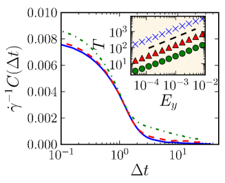
Figure 2: Properties of the mechanical noise experienced by a block. Two-time autocorrelation function of its xy-component, $C\left(\Delta t\right)\equiv\left\langle\delta\dot{\sigma}_{xy}\left(t\right)\delta\dot{\sigma}_{xy}\left(t+\Delta t\right)\right\rangle$, at shear rates $\dot{\gamma}=$ (solid blue line) $10^{-4}$, (dashed red line) $10^{-3}$, and (dash-dotted green line) $6\cdot 10^{-3}$. (Inset) Hopping time vs. energy barrier $E_{y}$ at $\dot{\gamma}=$ ($\color[rgb]{0,0,1}\times$) $10^{-4}$, ($\color[rgb]{1,0,0}\blacktriangle$) $10^{-3}$, and ($\color[rgb]{0,0.5,0}\bullet$) $6\cdot 10^{-3}$. The dashed line has a slope of 0.75. System size: 256x256. Note that the use of fictitious blocks (see text) allows to test potential barriers $E_{y}<E_{y}^{min}$.

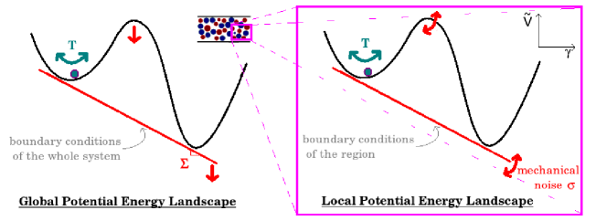
Figure 3: Schematic representation of the difference between thermal fluctuations and mechanical noise fluctuations in the PEL perspective.

To explore the question more thoroughly, we keep track of the mechanical noise fluctuations (per unit time) $\boldsymbol{\delta\dot{\sigma}}$ that a randomly selected block experiences, i.e., the fluctuations of the nonlocal terms in eq. 2. We then study the yielding time $T\left(E_{y}\right)$ of a fictitious block subject only to this mechanical noise, as a function of its energy barrier $E_{y}$, by measuring how long one has to wait before its elastic energy, $\frac{1}{4\mu}\left\|\int_{0}^{t}\boldsymbol{\delta\dot{\sigma}}(t^{\prime})dt^{\prime}\right\|^{2}$, grows larger than $E_{y}$. Note that only the mechanical noise fluctuations can act as “random kicks”; the average value, which is proportional to $\dot{\gamma}$, ought to be treated separately, as a drift term.

The two-time autocorrelation function of the steady-state fluctuations $\delta\dot{\sigma}_{xy}(i,j)$ of $\sigma_{xy}(i,j)$, shown in fig. 2, displays a fast initial decay, with a decay time similar to the plastic event lifetime. A small fraction, however, remains correlated over much longer times, which we tentatively ascribe to long-lived correlations in the yield stresses of nearby blocks, the latter being renewed only every $\gamma_{y}\dot{\gamma}^{-1}$. The magnitude of $\delta\dot{\sigma}_{xy}$ naturally increases with the number of simultaneous plastic events, and therefore with $\dot{\gamma}$. Turning to the escape time $T\left(E_{y}\right)$, the data plotted in fig. 2 rule out the Arrhenius law characteristic of activated processes, i.e.,

$$T\left(E_{y}\right)\propto e^{\frac{E_{y}}{x}}.$$ (4)

Instead, they are in favour of a hyperdiffusive process, with a power-law scaling $T\sim E_{y}^{0.75}\sim\sigma_{y}^{1.5}$.

How general are these findings? Let us recall that, in the theory of activated processes, a transition is completed when thermal fluctuations $\boldsymbol{f_{\mathrm{th}}}$ have pushed the system all the way up a potential barrier, in a fixed PEL $V({\bf x})$ [39]. Here, ${\bf x}$ is a high-dimensional vector containing the positions of all particles. For concreteness, consider the Langevin equation of motion in the overdamped regime,

$$0=-\zeta\frac{d{\bf x}}{dt}(t)-\nabla_{{\bf x}}V({\bf x})+\boldsymbol{f_{\mathrm{th}}}(t),$$ (5)

where $\zeta$ is a friction coefficient, $\langle\boldsymbol{f_{\mathrm{th}}}(t)\rangle={\bf 0}$, and $\langle\boldsymbol{f_{\mathrm{th}}}(t)\otimes\boldsymbol{f_{\mathrm{th}}}(t^{\prime})\rangle=2\zeta k_{B}T\delta(t-t^{\prime})\mathbb{I}$ (where $\mathbb{I}$ is the identity matrix). The exponential dependence in the Arrhenius law, eq. 4, hinges on the presence of recoil forces $-\nabla_{{\bf x}}V$ that constantly oppose the uphill motion. In contrast, mechanical noise fluctuations due to irreversible rearrangements cause persistent changes to the boundary conditions of the region of interest, thereby durably altering its PEL and stable points. Of course, transient effects, such as temporary dilation or inertial vibrations [40], may also occur during plastic events, but, being temporary, they will be subdominant, at least for large energy barriers.

The disparity between thermal fluctuations and mechanical noise is schematically illustrated in fig. 3, in which ${\bf x}$ is substituted by a scalar reaction coordinate, the shear strain $\gamma$. In this picture, mechanical noise acts as a “random” external stress, which tilts the potential $V(\gamma)$ of the region (supposed of unit volume) [41] into $\tilde{V}(\gamma,t)\equiv V(\gamma)-\gamma\sigma(t)$, where $\sigma(t)=\langle\dot{\sigma}\rangle t+f_{\mathrm{mec}}(t)$, with the shorthand $f_{\mathrm{mec}}(t)\equiv\int_{0}^{t}\delta\dot{\sigma}(\tau)d\tau$, is the stress applied at the boundary of the region. We examine the effect of $f_{\mathrm{mec}}(t)$, i.e., the fluctuations around the drift term $\langle\dot{\sigma}\rangle t$. Under their influence, energy barriers wax and wane, and their flattening out, signalling a plastic event, is therefore similar to a first passage time problem in a simple diffusion process over a flat landscape. More formally, after inclusion of the mechanical noise, eq. 5 turns into

$$0=-\zeta\frac{d\gamma}{dt}(t)-\frac{dV}{d\gamma}[\gamma(t)]+\langle\dot{\sigma}\rangle t+f_{\mathrm{mec}}(t)+f_{\mathrm{th}}(t).$$ (6)

Mechanical noise and thermal fluctuations differ in that

$$\langle f_{\mathrm{th}}(t)f_{\mathrm{th}}(t^{\prime})\rangle\propto\delta(t-t^{\prime}),$$ (7)

whereas

$$\langle f_{\mathrm{mec}}(t)f_{\mathrm{mec}}(t^{\prime})\rangle\ =\int_{0}^{t}d\tau\int_{0}^{t^{\prime}}d\tau^{\prime}C(\tau-\tau^{\prime}).$$ (8)

When the autocorrelation function $C(\Delta t)\equiv\langle\delta\dot{\sigma}(t)\delta\dot{\sigma}(t+\Delta t)\rangle$ decays quickly to zero, then $\langle f_{\mathrm{mec}}(t)f_{\mathrm{mec}}(t^{\prime})\rangle\sim\mathrm{min}(t,t^{\prime})$, and it follows that the energy barrier flattens out under the sole influence of $f_{\mathrm{mec}}$, i.e., $\mathrm{max}\ d\tilde{V}/d\gamma\rightarrow 0$, after a time $T\sim(\mathrm{max}\ dV/d\gamma)^{2}\equiv\sigma_{y}^{2}$. This purely diffusive case is encountered in Picard’s model (data not shown). For the model that we introduced previously, the process was in fact hyperdiffusive, owing to the presence of slowly decaying correlations of the noise. In any case, the escape occurs much faster than in an activated process.

This result may seem at odds with the numerical observation of activated processes in similar situations in ref. [42]. In this paper the inversion rate of a two-state system weakly coupled to a simple shear flow was observed to depend exponentially on the energy barrier $V_{0}$ between the two states, with an activation temperature $x>T_{bath}$, the bath temperature. The apparent contradiction vanishes as soon as one notices that in the specific protocol used in ref. [42] the internal potential energy $V(u)$ is not durably altered by the mechanical noise. As a matter of fact, a similar idea can be carried out within the framework of our model and it also yields an exponential variation of the hopping rate with $V_{0}$.

At this stage, we must say that our conclusions concerning the (non)existence of a mechanical noise temperature have, a priori, no bearing on some other definitions of an effective temperature, such as those based upon fluctuation-dissipation theorems [43, 44], or the effective temperature in the Shear Transformation Zone theory, which gives a measure of “disorder” fluctuations in space, regardless of their variations in time [45].

In conclusion, in the widely accepted scenario for the flow of amorphous solids, a non constant flow curve in an athermal system implies the existence of an interplay between the (cascades of) local particle rearrangements and the driving velocity. This interplay leads to a stress increase even when a large difference exists between the duration of a single plastic event and the inverse shear rate. The interplay mechanism differs from the widespread reliance on effective activation phenomena triggered by mechanical noise to explain the flow curve. If the onset of local yield is controlled by a parameter akin to local stress or strain, mechanical noise fluctuations due to distant plastic events and thermal fluctuations lead to different barrier-crossing statistics.

In the light of these findings, modifications of models such as SGR or Hébraud-Lequeux could be considered. Indeed, a simple fit of the flow curve does not establish the validity of a model or the correct assessment of the statistical properties of the mechanical noise. For a full characterisation of these properties, microscopic models or particle-resolved experiments may prove necessary.

- [1] \NamePrincen H. Kiss A. \REVIEWJournal of colloid and interface science1281989176.
- [2] \NameBécu L., Manneville S. Colin A. \REVIEWPhysical Review Letters962006.
- [3] \NameLemaître A. Caroli C. \REVIEWPhysical review letters1032009065501.
- [4] \NameSchall P. van Hecke M. \REVIEWAnnual Review of Fluid Mechanics42201067.
- [5] \NameKatgert G., Tighe B. P., Möbius M. E. van Hecke M. \REVIEWEPL (Europhysics Letters)90201054002.
- [6] \NameJop P., Mansard V., Chaudhuri P., Bocquet L. Colin A. \REVIEWPhysical Review Letters1082012148301.
- [7] \NameArgon A. Kuo H. \REVIEWMaterials Science and Engineering391979101.
- [8] \NameHébraud P., Lequeux F., Munch J. Pine D. \REVIEWPhysical Review Letters7819974657.
- [9] \NameMaloney C. E. Lemaître A. \REVIEWPhysical Review E742006016118.
- [10] \NameAmon A., Bruand A., Crassous J., Clément E. et al. \REVIEWPhysical review letters1082012135502.
- [11] \NameBulatov V. V. Argon A. S. \REVIEWModelling and Simulation in Materials Science and Engineering21994167.
- [12] \NameSollich P., Lequeux F., Hébraud P. Cates M. E. \REVIEWPhysical Review Letters7819972020.
- [13] \NamePicard G., Ajdari A., Lequeux F. Bocquet L. \REVIEWPhysical Review E712005010501.
- [14] \NameBocquet L., Colin A. Ajdari A. \REVIEWPhysical review letters1032009036001.
- [15] \NameHomer E. R. Schuh C. A. \REVIEWActa Materialia5720092823.
- [16] \NameDahmen K. A., Ben-Zion Y. Uhl J. T. \REVIEWNature Physics72011554.
- [17] \NameVandembroucq D. Roux S. \REVIEWPhysical Review B842011134210.
- [18] \NameIkeda A., Berthier L. Sollich P. \REVIEWPhysical Review Letters1092012018301.
- [19] \NameNicolas A. Barrat J.-L. \REVIEWFaraday Discuss.1672013567.
- [20] \NameChattoraj J., Caroli C. Lemaître A. \REVIEWPhysical Review E842011011501.
- [21] \NameTighe B. P., Woldhuis E., Remmers J. J. C., van Saarloos W. van Hecke M. \REVIEWPhysical Review Letters1052010088303.
- [22] \NameBoyer F., Guazzelli E. Pouliquen O. \REVIEWPhysical Review Letters1072011188301.
- [23] \NameTsamados M. \REVIEWThe European Physical Journal E322010165.
- [24] \NameOlsson P. Teitel S. \REVIEWPhysical Review Letters1092012108001.
- [25] \NameHébraud P. Lequeux F. \REVIEWPhysical Review Letters8119982934.
- [26] \NameMartens K., Bocquet L. Barrat J.-L. \REVIEWSoft Matter820124197.
- [27] \NameNicolas A., Martens K., Bocquet L. Barrat J.-L. \REVIEWSoft Matter2014, DOI: 10.1039/c4sm00395k.
- [28] \NameEshelby J. D. \REVIEWProceedings of the Royal Society A: Mathematical, Physical and Engineering Sciences2411957376.
- [29] \NameSchall P., Weitz D. A. Spaepen F. \REVIEWScience (New York, N.Y.)31820071895.
- [30] \NamePuosi F., Rottler J. Barrat J.-L. \REVIEWPhys. Rev. E892014042302.
- [31] \NameZargar R., Nienhuis B., Schall P. Bonn D. \REVIEWPhysical Review Letters1102013258301.
- [32] \NameDoliwa B. Heuer A. \REVIEWPhysical Review E672003031506.
- [33] \NameHeuer A. \REVIEWJournal of Physics: Condensed Matter202008373101.
- [34] \NameSollich P. \REVIEWPhysical Review E581998738.
- [35] \NameFielding S., Sollich P. Cates M. \REVIEWJournal of Rheology442000323.
- [36] \NamePouliquen O. Gutfraind R. \REVIEWPhysical Review E531996552.
- [37] \NameBehringer R., Bi D., Chakraborty B., Henkes S. Hartley R. \REVIEWPhysical Review Letters1012008268301.
- [38] \NameReddy K. A., Forterre Y. Pouliquen O. \REVIEWPhysical Review Letters1062011108301.
- [39] \NameKramers H. A. \REVIEWPhysica71940284.
- [40] \NameSalerno K., Maloney C. E. Robbins M. O. \REVIEWPhysical Review Letters1092012105703.
- [41] \NameGagnon G., Patton J. Lacks D. J. \REVIEWPhysical Review E642001051508.
- [42] \NameIlg P. Barrat J.-L. \REVIEWEurophysics Letters (EPL)79200726001.
- [43] \NameBerthier L., Barrat J.-L. Kurchan J. \REVIEWPhysical Review E6120005464.
- [44] \NameHaxton T. K. Liu A. J. \REVIEWPhysical Review Letters992007195701.
- [45] \NameBouchbinder E., Langer J. Procaccia I. \REVIEWPhysical Review E752007036107.