A Fourier Pseudospectral Method for the “Good” Boussinesq Equation with Second Order Temporal Accuracy

Abstract

In this paper, we discuss the nonlinear stability and convergence of a fully discrete Fourier pseudospectral method coupled with a specially designed second order time-stepping for the numerical solution of the “good” Boussinesq equation. Our analysis improves the existing results presented in earlier literature in two ways. First, an $\ell^{\infty}(0,T^{*};H^{2})$ convergence for the solution and $\ell^{\infty}(0,T^{*};\ell^{2})$ convergence for the time-derivative of the solution are obtained in this paper, instead of the $\ell^{\infty}(0,T^{*};\ell^{2})$ convergence for the solution and the $\ell^{\infty}(0,T^{*};H^{-2})$ convergence for the time-derivative, given in [17]. In addition, the stability and convergence of this method is shown to be unconditional for the time step in terms of the spatial grid size, compared with a severe restriction time step restriction $\Delta t\leq Ch^{2}$ reported in [17].

Keywords: Good Boussinesq equation, fully discrete Fourier pseudospectral method, aliasing error, stability and convergence

AMS subject classification: 65M12, 65M70

1 Introduction

The soliton-producing nonlinear wave equation is a topic of significant scientific interest. One commonly used example is the so-called “good” Boussinesq (GB) equation

$$u_{tt}=-u_{xxxx}+u_{xx}+(u^{p})_{xx},\quad\mbox{with an integer $p\geq 2$}.$$ (1.1)

It is similar to the well-known Korteweg-de Vries (KdV) equation; a balance between dispersion and nonlinearity leads to the existence of solitons. The GB equation and its various extensions have been investigated by many authors. For instance, a closed form solution for the two soliton interaction of Eq. (1.1) was obtained by Manoranjan et al. in [36] and a few numerical experiments were performed based on the Petrov-Galerkin method with linear “hat” functions. In [37], it was shown that the GB equation possesses a highly complicated mechanism for the solitary waves interaction. Ortega and Sanz-Serna [39] discussed nonlinear stability and convergence of some simple finite difference schemes for the numerical solution of this equation. More analytical and numerical works related to GB equations can be found in the literature, for example [1, 4, 5, 10, 11, 16, 17, 19, 29, 38, 40, 47].

In this paper, we consider the GB equation (1.1), with a periodic boundary condition over an 1-D domain $\Omega=(0,L)$ and initial data $u(x,0)=u^{0}(x)$, $u_{t}(x,0)=v^{0}(x)$, both of which are $L$-periodic. It is assumed that a unique, periodic, smooth enough solution exists for (1.1) over the time interval $(0,T)$. This $L$-periodicity assumption is reasonable if the solution to (1.1) decays exponentially outside $[0,L]$.

Due to the periodic boundary condition, the Fourier collocation (pseudospectral) differentiation is a natural choice to obtain the optimal spatial accuracy. There has been a wide and varied literature on the development of spectral and pseudospectral schemes. For instance, the stability analysis for linear time-dependent problems can be found in [18, 35], etc, based on eigenvalue estimates. Some pioneering works for nonlinear equations were initiated by Maday and Quarteroni [32, 33, 34] for steady-state spectral solutions. Also note the analysis of one-dimensional conservation laws by Tadmor and collaborators [9, 23, 31, 43, 44, 45, 46], semi-discrete viscous Burgers’ equation and Navier-Stokes equations by E [13, 14], the Galerkin spectral method for Navier-Stokes equations led by Guo [20, 21, 22, 23] and Shen [12, 24], and the fully discrete (discrete both in space and time) pseudospectral method applied to viscous Burgers’ equation in [19] by Gottlieb and Wang and [6] by Bressan and Quarteroni, etc.

Most of the theoretical developments in nonlinear spectral and pseudospectral schemes are related to a parabolic PDE, in which the diffusion term plays a key role in the stability and convergence analysis. Very few works have analyzed a fully discrete pseudospectral method applied to a nonlinear hyperbolic PDE. Among the existing ones, it is worth mentioning Frutos et al.’s work [17] on the nonlinear analysis of a second order (in time) pseudospectral scheme for the GB equation (with $p=2$). However, as the authors point out in their remark on page 119, these theoretical results were not optimal: “ … our energy norm is an $L^{2}$-norm of $u$ combined with a negative norm of $u_{t}$. This should be compared with the energy norm in [30]: there, no integration with respect to $x$ is necessary and convergence is proved in $H^{2}$ for $u$ and $L^{2}$ for $u_{t}$”. The difficulties in the analysis are due to the absence of a dissipation mechanism in the GB equation (1.1), which makes the nonlinear error terms much more challenging to analyze than that of a parabolic equation. The presence of a second order spatial derivative for the nonlinear term leads to an essential difficulty of numerical error estimate in a higher order Sobolev norm. In addition to the lack of optimal numerical error estimate, [17] also imposes a severe time step restriction: $\Delta t\leq Ch^{2}$ (with $C$ a fixed constant), in the nonlinear stability analysis. Such a constraint becomes very restrictive for a fine numerical mesh and leads to a high computational cost.

In this work we propose a second order (in time) pseudospectral scheme for the the GB equation (1.1) with an alternate approach, and provide a novel nonlinear analysis. In more detail, an $\ell^{\infty}(0,T^{*};H^{2})$ convergence for $u$ and $\ell^{\infty}(0,T^{*};\ell^{2})$ convergence for $u_{t}$ are derived, compared with the $\ell^{\infty}(0,T^{*};\ell^{2})$ convergence for $u$ and $\ell^{\infty}(0,T^{*};H^{-2})$ convergence for $u_{t}$, as reported in [17]. Furthermore, such a convergence is unconditional (for the time step $\Delta t$ in terms of space grid size $h$) so that the severe time step constraint $\Delta t\leq Ch^{2}$ is avoided.

The methodology of the proposed second order temporal discretization is very different from that in [17]. To overcome the difficulty associated with the second order temporal derivative in the hyperbolic equation, we introduce a new variable $\psi$ to approximate $u_{t}$, which greatly facilitates the numerical implementation. On the other hand, the corresponding second order consistency analysis becomes non-trivial because of an $O(\Delta t^{2})$ numerical error between the centered difference of $u$ and the mid-point average of $\psi$. Without a careful treatment, such an $O(\Delta t^{2})$ numerical error might seem to introduce a reduction of temporal accuracy, because of the second order time derivative involved in the equation. To overcome this difficulty, we perform a higher order consistency analysis by an asymptotic expansion; as a result, the constructed approximate solution satisfies the numerical scheme with a higher order truncation error. Furthermore, a projection of the exact solution onto the Fourier space leads to an optimal regularity requirement.

For the nonlinear stability and convergence analysis, we have to obtain a direct estimate of the (discrete) $H^{2}$ norm of the nonlinear numerical error function. This estimate relies on the aliasing error control lemma for pseudospectral approximation to nonlinear terms, which was proven in a recent work [19]. That’s the key reason why we are able to overcome the key difficulty in the nonlinear estimate and obtain an $\ell^{\infty}(0,T^{*};H^{2})$ convergence for $u$ and $\ell^{\infty}(0,T^{*};\ell^{2})$ convergence for $u_{t}$. We prove that the proposed numerical scheme is fully consistent (with a higher order expansion), stable and convergent in the $H^{2}$ norm up to some fixed final time $T^{*}$. In turn, the maximum norm bound of the numerical solution is automatically obtained, because of the $H^{2}$ error estimate and the corresponding Sobolev embedding. Therefore, the inverse inequality in the stability analysis is not needed and any scaling law between $\Delta t$ and $h$ is avoided, compared with the $\Delta t\leq Ch^{2}$ constraint reported in [17].

This paper is outlined as follows. In Section 2 we review the Fourier spectral and pseudospectral differentiation, recall an aliasing error control lemma (proven in [19]), and present an alternate second order (in time) pseudospectral scheme for the GB equation (1.1). In Section 3, the consistency analysis of the scheme is studied in detail. The stability and convergence analysis is reported in Section 4. A simple numerical result is presented in Section 5. Finally, some concluding remarks are made in Section 6.

2 The Numerical Scheme

2.1 Review of Fourier spectral and pseudospectral approximations

For $f(x)\in L^{2}(\Omega)$, $\Omega=(0,L)$, with Fourier series

$$f(x)=\sum_{l=-\infty}^{\infty}\hat{f}_{l}{\rm e}^{2\pi{\rm i}lx/L},\quad\mbox{with}\quad\hat{f}_{l}=\int_{\Omega}f(x){\rm e}^{-2\pi{\rm i}lx/L}dx,$$ (2.2)

its truncated series is defined as the projection onto the space ${\cal B}^{N}$ of trigonometric polynomials in $x$ of degree up to $N$, given by

$${\cal P}_{N}f(x)=\sum_{l=-N}^{N}\hat{f}_{l}{\rm e}^{2\pi{\rm i}lx/L}.$$ (2.3)

To obtain a pseudospectral approximation at a given set of points, an interpolation operator ${\cal I}_{N}$ is introduced. Given a uniform numerical grid with $(2N+1)$ points and a discrete vector function ${\mathbf{f}}$ where ${\mathbf{f}}_{i}=f(x_{i})$, for each spatial point $x_{i}$. The Fourier interpolation of the function is defined by

$$\left({\cal I}_{N}f\right)(x)=\sum_{l=-N}^{N}(\hat{f}_{c}^{N})_{l}{\rm e}^{2\pi{\rm i}lx/L},$$ (2.4)

where the $(2N+1)$ pseudospectral coefficients $(\hat{f}_{c}^{N})_{l}$ are computed based on the interpolation condition $f(x_{i})=\left({\cal I}_{N}f\right)(x_{i})$ on the $2N+1$ equidistant points [3, 7, 26]. These collocation coefficients can be efficiently computed using the fast Fourier transform (FFT). Note that the pseudospectral coefficients are not equal to the actual Fourier coefficients; the difference between them is known as the aliasing error. In general, ${\cal P}_{N}f(x)\neq{\cal I}_{N}f(x)$, and even ${\cal P}_{N}f(x_{i})\neq{\cal I}_{N}f(x_{i})$, except of course in the case that $f\in{\cal B}^{N}$.

The Fourier series and the formulas for its projection and interpolation allow one to easily take derivative by simply multiplying the appropriate Fourier coefficients $(\hat{f}_{c}^{N})_{l}$ by $2l\pi{\rm i}/L$. Furthermore, we can take subsequent derivatives in the same way, so that differentiation in physical space is accomplished via multiplication in Fourier space. As long as $f$ and all is derivatives (up to $m$-th order) are continuous and periodic on $\Omega$, the convergence of the derivatives of the projection and interpolation is given by

$$\|\partial^{k}f(x)-\partial^{k}{\cal P}_{N}f(x)\| \leq C\|f^{(m)}\|h^{m-k},\quad\mbox{for}\,\,\,0\leq k\leq m,$$

$$\|\partial^{k}f(x)-\partial^{k}{\cal I}_{N}f(x)\| \leq C\|f\|_{H^{m}}h^{m-k},\quad\mbox{for}\,\,\,0\leq k\leq m,\,m>\frac{d}{2},$$ (2.5)

in which $\|\cdot\|$ denotes the $L^{2}$ norm. For more details, see the discussion of approximation theory by Canuto and Quarteroni [8] .

For any collocation approximation to the function $f(x)$ at the points $x_{i}$

$$f(x_{i})=\left({\cal I}_{N}f\right)_{i}=\sum_{l=-N}^{N}(\hat{f}_{c}^{N})_{l}{\rm e}^{2\pi{\rm i}lx_{i}},$$ (2.6)

one can define discrete differentiation operator ${\cal D}_{N}$ operating on the vector of grid values ${\mathbf{f}}=f(x_{i})$. In practice, one may compute the collocation coefficients $(\hat{f_{c}^{N})}_{l}$ via FFT, and then multiply them by the correct values (given by $2l\pi{\rm i}$) and perform the inverse FFT. Alternatively, we can view the differentiation operator ${\cal D}_{N}$ as a matrix, and the above process can be seen as a matrix-vector multiplication. The same process is performed for the second and fourth derivatives $\partial_{x}^{2}$, $\partial_{x}^{4}$, where this time the collocation coefficients are multiplied by $(-4\pi^{2}l^{2}/L^{2})$ and $(16\pi^{4}l^{4}/L^{4})$, respectively. In turn, the differentiation matrix can be applied for multiple times, i.e. the vector ${\mathbf{f}}$ is multiplied by ${\cal D}^{2}_{N}$ and ${\cal D}_{N}^{4}$, respectively.

Since the pseudospectral differentiation is taken at a point-wise level, a discrete $L^{2}$ norm and inner product need to be introduced to facilitate the analysis. Given any periodic grid functions ${\mathbf{f}}$ and ${\mathbf{g}}$ (over the numerical grid), we note that these are simply vectors and define the discrete $L^{2}$ inner product and norm

$$\left\|{\mathbf{f}}\right\|_{2}=\sqrt{\left\langle{\mathbf{f}},{\mathbf{f}}\right\rangle},\quad\mbox{with}\quad\left\langle{\mathbf{f}},{\mathbf{g}}\right\rangle=\frac{1}{2N+1}\sum_{i=0}^{2N}{\mathbf{f}}_{i}{\mathbf{g}}_{i}.$$ (2.7)

The following summation by parts (see [19]) will be of use:

$$\left\langle{\mathbf{f}},{\cal D}_{N}{\mathbf{g}}\right\rangle=-\left\langle{\cal D}_{N}{\mathbf{f}},{\mathbf{g}}\right\rangle,\quad\left\langle{\mathbf{f}},{\cal D}_{N}^{2}{\mathbf{g}}\right\rangle=-\left\langle{\cal D}_{N}{\mathbf{f}},{\cal D}_{N}{\mathbf{g}}\right\rangle,\quad\left\langle{\mathbf{f}},{\cal D}_{N}^{4}{\mathbf{g}}\right\rangle=\left\langle{\cal D}_{N}^{2}{\mathbf{f}},{\cal D}_{N}^{2}{\mathbf{g}}\right\rangle.$$ (2.8)

2.2 An aliasing error control estimate in Fourier pseudospectral approximation

This lemma, established in [19], allows us to bound the aliasing error for the nonlinear term, and will be critical to our analysis. For any function $\varphi(x)$ in the space ${\cal B}^{pN}$, its collocation coefficients $\hat{q}^{N}_{l}$ are computed based on the $2N+1$ equidistant points. In turn, ${\cal I}_{N}\varphi(x)$ is given by the continuous expansion based on these coefficients:

$${\cal I}_{N}\varphi(x)=\sum_{l=-N}^{N}\hat{q}^{N}_{l}{\rm e}^{2\pi{\rm i}lx/L}.$$ (2.9)

Since $\varphi(x)\in{\cal B}^{pN}$, we have ${\cal I}_{N}\varphi(x)\neq{\cal P}_{N}\varphi(x)$ due to the aliasing error.

The following lemma enables us to obtain an $H^{m}$ bound of the interpolation of the nonlinear term; the detailed proof can be found in [19].

Lemma 2.1.

For any $\varphi\in{\cal B}^{pN}$ (with $p$ an integer) in dimension $d$, we have

$$\left\|{\cal I}_{N}\varphi\right\|_{H^{k}}\leq\left(\sqrt{p}\right)^{d}\left\|\varphi\right\|_{H^{k}}.$$ (2.10)

2.3 Formulation of the numerical scheme

We propose the following fully discrete second order (in time) scheme for the equation (1.1):

$$\left\{\begin{array}[]{rl}\displaystyle\vspace{.05in}\frac{\psi^{n+1}-\psi^{n}}{\Delta t}=&-D_{N}^{4}\left(\frac{u^{n+1}+u^{n}}{2}\right)+D_{N}^{2}\left(\frac{u^{n+1}+u^{n}}{2}\right)\\ \vspace{.05in}\displaystyle\hfil&+D_{N}^{2}\left(\frac{3}{2}(u^{n})^{p}-\frac{1}{2}(u^{n-1})^{p}\right),\\ \displaystyle\vspace{.05in}\frac{u^{n+1}-u^{n}}{\Delta t}=&\frac{\psi^{n+1}+\psi^{n}}{2},\end{array}\right.$$ (2.11)

where $\psi$ is a second order approximation to $u_{t}$ and $D_{N}$ denotes the discrete differentiation operator.

Remark 2.2.

With a substitution $\psi^{n+1}=\frac{2(u^{n+1}-u^{n})}{\Delta t}-\psi^{n}$, the scheme (2.11) can be reformulated as a closed equation for $u^{n+1}$:

$$\frac{2u^{n+1}}{\Delta t^{2}}+\frac{1}{2}\left(D_{N}^{4}-D_{N}^{2}\right)u^{n+1} = D_{N}^{2}\left(\frac{3}{2}(u^{n})^{p}-\frac{1}{2}(u^{n-1})^{p}\right)-\frac{1}{2}\left(D_{N}^{4}-D_{N}^{2}\right)u^{n}$$ (2.12)

$$+\frac{\frac{2u^{n}}{\Delta t}+2\psi^{n}}{\Delta t}.$$

Since the treatment of the nonlinear term is fully explicit, this resulting implicit scheme requires only a linear solver. Furthermore, a detailed calculation shows that all the eigenvalues of the linear operator on the left hand side are positive, and so the unique unconditional solvability of the proposed scheme (2.11) is assured. In practice, the FFT can be utilized to efficiently obtain the numerical solutions.

Remark 2.3.

An introduction of the variable $\psi$ not only facilitates the numerical implementation, but also improves the numerical stability, due to the fact that only two consecutive time steps $t^{n}$, $t^{n+1}$, are involved in the second order approximation to $u_{tt}$. In contrast, three time steps $t^{n+1}$, $t^{n}$ and $t^{n-1}$ are involved in the numerical approximation to the second order temporal derivative as presented in the earlier work [17] (with $p=2$):

$$\frac{u^{n+1}-2u^{n}+u^{n-1}}{\Delta t^{2}}=-\frac{1}{4}D_{N}^{4}\left(u^{n+1}+2u^{n}+u^{n-1}\right)+D_{N}^{2}u^{n}+D_{N}^{2}\left((u^{n})^{2}\right).$$ (2.13)

A careful numerical analysis in [17] shows that the numerical stability for (2.13) is only valid under a severe time step constraint $\Delta t\leq Ch^{2}$, since this scheme is evaluated at the time step $t^{n}$. On the other hand, the special structure of our proposed scheme (2.11) results in an unconditional stability and convergence for a fixed final time, as will be presented in later analysis.

3 The Consistency Analysis

In this section we establish a truncation error estimate for the fully discrete scheme (2.11) for the GB equation (1.1). A finite Fourier projection of the exact solution is taken to the GB equation (1.1) and a local truncation error is derived. Moreover, we perform a higher order consistency analysis in time, through an addition of a correction term, so that the constructed of approximate solution satisfies the numerical scheme with higher order temporal accuracy. This approach avoids a key difficulty associated with the accuracy reduction in time due to the appearance of the second in time temporal derivative.

3.1 Truncation error analysis for $U_{N}$

Given the domain $\Omega=(0,L)$, the uniform mesh grid $(x_{i})$, $0\leq i\leq 2N$, and the exact solution $u_{\mbox{\tiny}e}$, we denote $U_{N}$ as its projection into ${\cal B}^{N}$:

$$U_{N}(x,t):={\cal P}_{N}u_{\mbox{\tiny}e}(x,t).$$ (3.1)

The following approximation estimates are clear:

$$\left\|U_{N}-u_{\mbox{\tiny}e}\right\|_{L^{\infty}(0,T^{*};H^{r})}\leq Ch^{m}\left\|u_{\mbox{\tiny}e}\right\|_{L^{\infty}(0,T^{*};H^{m+r})},\quad\mbox{for}\,\,\,r\geq 0,$$ (3.2)

$$\left\|\partial_{t}^{k}\left(U_{N}-u_{\mbox{\tiny}e}\right)\right\|_{H^{r}}\leq Ch^{m}\left\|\partial_{t}^{k}u_{\mbox{\tiny}e}\right\|_{H^{m+r}},\quad\mbox{for}\,\,\,r\geq 0,\,\,0\leq k\leq 4,$$ (3.3)

in which the second inequality comes from the fact that $\partial_{t}^{k}U_{N}$ is the truncation of $\partial_{t}^{k}u_{\mbox{\tiny}e}$ for any $k\geq 0$, since projection and differentiation commute:

$$\frac{\partial^{k}}{\partial t^{k}}U_{N}(\mbox{\boldmath$x$},t)=\frac{\partial^{k}}{\partial t^{k}}{\cal P}_{N}u_{\mbox{\tiny}e}(x,t)={\cal P}_{N}\frac{\partial^{k}u_{\mbox{\tiny}e}(x,t)}{\partial t^{k}}.$$ (3.4)

As a direct consequence, the following linear estimates are straightforward:

$$\left\|\partial_{t}^{2}\left(U_{N}-u_{\mbox{\tiny}e}\right)\right\|_{L^{2}} \leq Ch^{m}\left\|\partial_{t}^{2}u_{\mbox{\tiny}e}\right\|_{H^{m}},$$ (3.5)

$$\left\|\partial_{x}^{2}\left(U_{N}-u_{\mbox{\tiny}e}\right)\right\|_{L^{2}} \leq Ch^{m}\left\|u_{\mbox{\tiny}e}\right\|_{H^{m+2}},\quad\left\|\partial_{x}^{4}\left(U_{N}-u_{\mbox{\tiny}e}\right)\right\|_{L^{2}}\leq Ch^{m}\left\|u_{\mbox{\tiny}e}\right\|_{H^{m+4}}.$$ (3.6)

On the other hand, a discrete $\left\|\cdot\right\|_{2}$ estimate for these terms are needed in the local truncation derivation. To overcome this difficulty, we observe that

$$\left\|\partial_{t}^{2}\left(U_{N}-u_{\mbox{\tiny}e}\right)\right\|_{2}=\left\|{\cal I}_{N}\left(\partial_{t}^{2}\left(U_{N}-u_{\mbox{\tiny}e}\right)\right)\right\|_{L^{2}}\leq\left\|\partial_{t}^{2}\left(U_{N}-u_{\mbox{\tiny}e}\right)\right\|_{L^{2}}+\left\|\partial_{t}^{2}\left({\cal I}_{N}u_{\mbox{\tiny}e}-u_{\mbox{\tiny}e}\right)\right\|_{L^{2}},$$ (3.7)

in which the second step comes from the fact that ${\cal I}_{N}\partial_{t}^{2}U_{N}=\partial_{t}^{2}U_{N}$, since $\partial_{t}^{2}U_{N}\in{\cal B}^{N}$. The first term has an estimate given by (3.5), while the second term could be bounded by

$$\left\|\left(\partial_{t}^{2}\left({\cal I}_{N}u_{\mbox{\tiny}e}-u_{\mbox{\tiny}e}\right)\right)\right\|_{L^{2}}=\left\|{\cal I}_{N}\left(\partial_{t}^{2}u_{\mbox{\tiny}e}\right)-\partial_{t}^{2}u_{\mbox{\tiny}e}\right\|_{L^{2}}\leq Ch^{m}\left\|\partial_{t}^{2}u_{\mbox{\tiny}e}\right\|_{H^{m}},$$ (3.8)

as an application of (2.5). In turn, its combination with (3.7) and (3.5) yields

$$\left\|\partial_{t}^{2}\left(U_{N}-u_{\mbox{\tiny}e}\right)\right\|_{2}\leq Ch^{m}\left\|\partial_{t}^{2}u_{\mbox{\tiny}e}\right\|_{H^{m}}.$$ (3.9)

Using similar arguments, we also arrive at

$$\left\|\partial_{x}^{2}\left(U_{N}-u_{\mbox{\tiny}e}\right)\right\|_{2}\leq Ch^{m}\left\|u_{\mbox{\tiny}e}\right\|_{H^{m+2}},\quad\left\|\partial_{x}^{4}\left(U_{N}-u_{\mbox{\tiny}e}\right)\right\|_{2}\leq Ch^{m}\left\|u_{\mbox{\tiny}e}\right\|_{H^{m+4}}.$$ (3.10)

For the nonlinear term, we begin with the following expansion:

$$\partial_{x}^{2}\left(u_{\mbox{\tiny}e}^{p}\right) = p\left((p-1)u_{\mbox{\tiny}e}^{p-2}(u_{\mbox{\tiny}e})_{x}^{2}+u_{\mbox{\tiny}e}^{p-1}(u_{\mbox{\tiny}e})_{xx}\right),\quad\mbox{which in turn gives}$$

$$\partial_{x}^{2}\left(u_{\mbox{\tiny}e}^{p}-(U_{N})^{p}\right) = p\Bigl{(}(p-1)U_{N}^{p-2}(u_{\mbox{\tiny}e}+U_{N})_{x}(u_{\mbox{\tiny}e}-U_{N})_{x}$$ (3.11)

$$+(p-1)(u_{\mbox{\tiny}e}-U_{N})(u_{\mbox{\tiny}e})_{x}^{2}\sum_{k=0}^{p-3}u_{\mbox{\tiny}e}^{k}U_{N}^{p-3-k}$$

$$+U_{N}^{p-1}(u_{\mbox{\tiny}e}-U_{N})_{xx}+(u_{\mbox{\tiny}e}-U_{N})(u_{\mbox{\tiny}e})_{xx}\sum_{k=0}^{p-2}u_{\mbox{\tiny}e}^{k}U_{N}^{p-2-k}\Bigr{)}.$$

Subsequently, its combination with (3.2) implies that

$$\left\|\partial_{x}^{2}\left(u_{\mbox{\tiny}e}^{p}-(U_{N})^{p}\right)\right\|_{L^{2}}$$ (3.12)

$$\leq C\Bigl{(}\left\|U_{N}\right\|_{L^{\infty}}^{p-2}\cdot\left\|u_{\mbox{\tiny}e}+U_{N}\right\|_{W^{1,\infty}}\cdot\left\|u_{\mbox{\tiny}e}-U_{N}\right\|_{H^{1}}+\left\|U_{N}\right\|_{L^{\infty}}^{p-1}\cdot\left\|u_{\mbox{\tiny}e}-U_{N}\right\|_{H^{2}}$$

$$+\left\|u_{\mbox{\tiny}e}-U_{N}\right\|_{L^{\infty}}\cdot\left(\left\|u_{\mbox{\tiny}e}\right\|_{L^{\infty}}^{p-2}+\left\|U_{N}\right\|_{L^{\infty}}^{p-2}\right)\cdot\left(\left\|u_{\mbox{\tiny}e}\right\|_{H^{2}}+\left\|u_{\mbox{\tiny}e}\right\|_{W^{1,4}}^{2}\right)\Bigr{)}$$

$$\leq C\Bigl{(}\left\|U_{N}\right\|_{H^{1}}^{p-2}\cdot\left\|u_{\mbox{\tiny}e}+U_{N}\right\|_{H^{2}}\cdot\left\|u_{\mbox{\tiny}e}-U_{N}\right\|_{H^{1}}+\left\|U_{N}\right\|_{H^{1}}^{p-1}\cdot\left\|u_{\mbox{\tiny}e}-U_{N}\right\|_{H^{2}}$$

$$+\left\|u_{\mbox{\tiny}e}-U_{N}\right\|_{H^{1}}\cdot\left(\left\|u_{\mbox{\tiny}e}\right\|_{H^{1}}^{p-2}+\left\|U_{N}\right\|_{H^{1}}^{p-2}\right)\cdot\left(\left\|u_{\mbox{\tiny}e}\right\|_{H^{2}}+\left\|u_{\mbox{\tiny}e}\right\|_{H^{2}}^{2}\right)\Bigr{)}$$

$$\leq C\left(\left\|u_{\mbox{\tiny}e}\right\|_{H^{2}}^{p}+\left\|U_{N}\right\|_{H^{2}}^{p}\right)\cdot\left\|u_{\mbox{\tiny}e}-U_{N}\right\|_{H^{2}}$$

$$\leq C\left\|u_{\mbox{\tiny}e}\right\|_{H^{2}}^{p}\cdot\left\|u_{\mbox{\tiny}e}-U_{N}\right\|_{H^{2}}\leq Ch^{m}\left\|u_{\mbox{\tiny}e}\right\|_{H^{2}}^{p}\cdot\left\|u_{\mbox{\tiny}e}\right\|_{H^{m+2}},$$

in which an 1-D Sobolev embedding was used in the second step.

The following interpolation error estimates can be derived in a similar way, based on (2.5):

$$\left\|\partial_{x}^{2}(u_{\mbox{\tiny}e}^{p})-{\cal I}_{N}\left(\partial_{x}^{2}(u_{\mbox{\tiny}e}^{p})\right)\right\|_{L^{2}} \leq Ch^{m}\left\|\partial_{x}^{2}(u_{\mbox{\tiny}e}^{p})\right\|_{H^{m}}\leq Ch^{m}\left\|u_{\mbox{\tiny}e}\right\|_{H^{2}}^{p}\cdot\left\|u_{\mbox{\tiny}e}\right\|_{H^{m+2}},$$ (3.13)

$$\left\|\partial_{x}^{2}(U_{N}^{p})-{\cal I}_{N}\left(\partial_{x}^{2}(U_{N}^{p})\right)\right\|_{L^{2}} \leq Ch^{m}\left\|\partial_{x}^{2}(U_{N}^{p})\right\|_{H^{m}}\leq Ch^{m}\left\|u_{\mbox{\tiny}e}\right\|_{H^{2}}^{p}\cdot\left\|u_{\mbox{\tiny}e}\right\|_{H^{m+2}}.$$ (3.14)

In turn, a combination of (3.12)-(3.14) implies the following estimate for the nonlinear term

$$\left\|\partial_{x}^{2}\left(u_{\mbox{\tiny}e}^{p}-(U_{N})^{p}\right)\right\|_{2} = \left\|{\cal I}_{N}\left(\partial_{x}^{2}\left(u_{\mbox{\tiny}e}^{p}-(U_{N})^{p}\right)\right)\right\|_{L^{2}}$$ (3.15)

$$\leq \left\|\partial_{x}^{2}\left(u_{\mbox{\tiny}e}^{p}-(U_{N})^{p}\right)\right\|_{L^{2}}+\left\|\partial_{x}^{2}(u_{\mbox{\tiny}e}^{p})-{\cal I}_{N}\left(\partial_{x}^{2}(u_{\mbox{\tiny}e}^{p})\right)\right\|_{L^{2}}$$

$$+\left\|\partial_{x}^{2}(U_{N}^{p})-{\cal I}_{N}\left(\partial_{x}^{2}(U_{N}^{p})\right)\right\|_{L^{2}}\leq Ch^{m}\left\|u_{\mbox{\tiny}e}\right\|_{H^{2}}^{p}\cdot\left\|u_{\mbox{\tiny}e}\right\|_{H^{m+2}}.$$

By observing (3.9), (3.10), (3.15), we conclude that $U_{N}$ satisfies the original GB equation (1.1) up to an $O(h^{m})$ (spectrally accurate) truncation error:

$$\partial_{t}^{2}U_{N}=-\partial_{x}^{4}U_{N}+\partial_{x}^{2}U_{N}+\partial_{x}^{2}(U_{N}^{p})+\tau_{0},\quad\mbox{with}\,\,\,\left\|\tau_{0}\right\|_{2}\leq Ch^{m}\left(\left\|u_{\mbox{\tiny}e}\right\|_{H^{2}}^{p}+1\right)\cdot\left\|u_{\mbox{\tiny}e}\right\|_{H^{m+4}}.$$ (3.16)

Moreover, we define the following profile, a second order (in time) approximation to $\partial_{t}u_{\mbox{\tiny}e}$:

$$\Psi_{N}(x,t):=\partial_{t}U_{N}(x,t)-\frac{\Delta t^{2}}{12}\partial_{t}^{3}U_{N}(x,t).$$ (3.17)

For any function $G=G(x,t)$, given $n>0$ , we define $G^{n}(x):=G(x,n\Delta t)$.

3.2 Truncation error analysis in time

For simplicity of presentation, we assume $T=K\Delta t$ with an integer $K$. The following two preliminary estimates are excerpted from a recent work [2], which will be useful in later consistency analysis.

Proposition 3.1.

[2] For $f\in H^{3}(0,T)$, we have

$$\left\|\tau^{t}f\right\|_{\ell^{2}(0,T)}\leq C\Delta t^{m}\left\|f\right\|_{H^{m+1}(0,T)},\quad\mbox{with}\quad\tau^{t}f^{n}=\frac{f^{n+1}-f^{n}}{\Delta t}-f^{\prime}(t^{n+1/2}),$$ (3.18)

for $0\leq m\leq 2$, where $C$ only depends on $T$, $\left\|\ \cdot\ \right\|_{\ell^{2}(0,T)}$ is a discrete $L^{2}$ norm (in time) given by $\left\|g\right\|_{\ell^{2}(0,T)}=\sqrt{\Delta t\sum_{n=0}^{K-1}\left(g^{n}\right)^{2}}$.

Proposition 3.2.

[2] For $f\in H^{2}(0,T)$, we have

$$\left\|D_{t/2}^{2}f\right\|_{\ell^{2}(0,T)}:=\left(\Delta t\sum_{n=0}^{K-1}\left(D_{t/2}^{2}f^{n+1/2}\right)^{2}\right)^{\frac{1}{2}}\leq C\left\|f\right\|_{H^{2}(0,T)},$$ (3.19)

$$\left\|D_{t}^{2}f\right\|_{\ell^{2}(0,T)}:=\left(\Delta t\sum_{n=0}^{K-1}\left(D_{t}^{2}f^{n}\right)^{2}\right)^{\frac{1}{2}}\leq C\left\|f\right\|_{H^{2}(0,T)},$$ (3.20)

$$\mbox{with}\quad D_{t/2}^{2}f^{n+1/2}=\frac{4\left(f^{n+1}-2f(\ \cdot\ ,t^{n+1/2})+f^{n}\right)}{\Delta t^{2}},\quad D_{t}^{2}f^{n}=\frac{f^{n+1}-2f^{n}+f^{n-1}}{\Delta t^{2}},$$

where $C$ only depends on $T$.

The following theorem is the desired consistency result. To simplify the presentation below, for the constructed solution $(U_{N},\psi_{N})$, we define its vector grid function $(U^{n},\Psi^{n})={\cal I}(U_{N},\psi_{N})$ as its interpolation: $U^{n}_{i}=U_{N}^{n}(x_{i},t^{n})$, $\Psi^{n}_{i}=\Psi_{N}^{n}(x_{i},t^{n})$.

Theorem 3.1.

Suppose the unique periodic solution for equation (1.1) satisfies the following regularity assumption

$$u_{\mbox{\tiny}e}\in H^{4}(0,T;L^{2})\cap L^{\infty}(0,T;H^{m+4})\cap H^{2}(0,T;H^{4}).$$ (3.21)

Set $(U_{N},\Psi_{N})$ as the approximation solution constructed by (3.1), (3.17) and let $(U,\Psi)$ as its discrete interpolation. Then we have

$$\left\{\begin{array}[]{rl}\displaystyle\vspace{.05in}\frac{\Psi^{n+1}-\Psi^{n}}{\Delta t}&=-D_{N}^{4}(\frac{U^{n+1}+U^{n}}{2})+D_{N}^{2}(\frac{U^{n+1}+U^{n}}{2})\\ \vspace{.05in}\displaystyle\hfil&+D_{N}^{2}\left(\frac{3}{2}(U^{n})^{p}-\frac{1}{2}(U^{n-1})^{p}\right)+\tau_{1}^{n},\\ \displaystyle\vspace{.05in}\frac{U^{n+1}-U^{n}}{\Delta t}&=\frac{\Psi^{n+1}+\Psi^{n}}{2}+\Delta t\tau_{2}^{n},\end{array}\right.$$ (3.22)

where $\tau_{i}^{k}$ satisfies

$$\left\|\tau_{i}\right\|_{\ell^{2}\left(0,T;\ell^{2}\right)}:=\left(\Delta t\sum_{k=0}^{K}\left\|\tau_{i}^{k}\right\|^{2}_{2}\right)^{\frac{1}{2}}\leq M\left(\Delta t^{2}+h^{m}\right),\quad i=1,2,$$ (3.23)

in which $M$ only depends on the regularity of the exact solution $u_{\mbox{\tiny}e}$.

Proof.

We define the following notation:

$$\begin{array}[]{rclrclrcl}F_{0}^{n+1/2}&=&\frac{U^{n+1}-U^{n}}{\Delta t}&,&\\ F_{1}^{n+1/2}&=&\frac{\Psi^{n+1}-\Psi^{n}}{\Delta t}&,&\quad F_{1e}^{n+1/2}&=&(\partial_{t}^{2}U_{N})(\cdot,t^{n+1/2}),\\ F_{2}^{n+1/2}&=&D_{N}^{4}U^{n+1/2}&,&\quad F_{2e}^{n+1/2}&=&(\partial_{x}^{4}U_{N})(\cdot,t^{n+1/2}),\\ F_{3}^{n+1/2}&=&D_{N}^{2}U^{n+1/2}&,&\quad F_{2e}^{n+1/2}&=&(\partial_{x}^{2}U_{N})(\cdot,t^{n+1/2}),\\ F_{4}^{n+1/2}&=&D_{N}^{2}(\frac{3}{2}(U^{p})^{n}-\frac{1}{2}(U^{p})^{n-1})&,&\quad F_{4e}^{n+1/2}&=&(\partial_{x}^{2}U_{N}^{2})(\cdot,t^{n+1/2}),\\ F_{5}^{n+1/2}&=&\frac{\Psi^{n+1}+\Psi^{n}}{2}&.&\\ \end{array}$$ (3.24)

Note that the quantities on the left side are defined on the numerical grid (in space) point-wise, while the ones on the right hand side are continuous functions.

To begin with, we look at the second order time derivative terms, $F_{1}$ and $F_{1e}$. From the definition (3.17), we get

$$F_{1}^{n+1/2}=\frac{\partial_{t}u_{N}^{n+1}-\partial_{t}u_{N}^{n}}{\Delta t}-\frac{\Delta t^{2}}{12}\frac{\partial_{t}^{3}u_{N}^{n+1}-\partial_{t}^{3}u_{N}^{n}}{\Delta t}:=F_{11}^{n+1/2}-\frac{\Delta t^{2}}{12}F_{12}^{n+1/2},$$ (3.25)

at a point-wise level, where $F_{11}$ and $F_{12}$ are the finite difference (in time) approximation to $\partial_{t}^{2}U_{N}$, $\partial_{t}^{4}U_{N}$, respectively. We define $F_{11e}$ and $F_{12e}$ in a similar way as (3.24), i.e.

$$F_{11e}^{n+1/2}=\partial_{t}^{2}U_{N}(\cdot,t^{n+1/2}),\quad F_{12e}^{n+1/2}=\partial_{t}^{4}U_{N}(\cdot,t^{n+1/2}).$$ (3.26)

The following estimates can be derived by using Proposition 3.1 (with $m=2$ and $m=0$):

$$\left\|F_{11}-F_{11e}\right\|_{\ell^{2}(0,T)}\leq C\Delta t^{2}\left\|U_{N}\right\|_{H^{4}(0,T)},\quad\left\|F_{12}-F_{12e}\right\|_{\ell^{2}(0,T)}\leq C\left\|U_{N}\right\|_{H^{4}(0,T)},$$ (3.27)

for each fixed grid point. This in turn yields

$$\left\|F_{1}-F_{1e}\right\|_{\ell^{2}(0,T)}\leq C\Delta t^{2}\left\|U_{N}\right\|_{H^{4}(0,T)}.$$ (3.28)

In turn, an application of discrete summation in $\Omega$ leads to

$$\left\|F_{1}-{\cal I}(F_{1e})\right\|_{\ell^{2}\left(0,T;\ell^{2}\right)}\leq C\Delta t^{2}\left\|U_{N}\right\|_{H^{4}(0,T;L^{2})}\leq C\Delta t^{2}\left\|u_{\mbox{\tiny}e}\right\|_{H^{4}(0,T;L^{2})},$$ (3.29)

due to the fact that $U_{N}\in{\cal B}^{N}$, and (3.3) was used in the second step.

For the terms $F_{2}$ and $F_{2e}$, we start from the following observation (recall that $U_{N}^{k+1/2}=\frac{U_{N}^{k+1}+U_{N}^{k}}{2}$)

$$\left\|F_{2}^{n+1/2}-{\cal I}\left(\partial_{x}^{4}U_{N}^{n+1/2}\right)\right\|_{2}\equiv 0,\quad\mbox{since $U_{N}^{n+1/2}\in{\cal B}^{N}$ }.$$ (3.30)

Meanwhile, a comparison between $U_{N}^{n+1/2}$ and $U_{N}(\cdot\ ,t^{n+1/2})$ shows that

$$U_{N}^{n+1/2}-U_{N}(\ \cdot\ ,t^{n+1/2})=\frac{1}{8}\Delta t^{2}D_{t/2}^{2}U_{N}^{n+1/2}.$$ (3.31)

Meanwhile, an application of Prop. 3.2 gives

$$\left\|D_{t/2}^{2}\partial_{x}^{4}U_{N}\right\|_{\ell^{2}(0,T)}\leq C\left\|\partial_{x}^{4}U_{N}\right\|_{H^{2}(0,T)},$$ (3.32)

at each fixed grid point. As a result, we get

$$\left\|F_{2}-{\cal I}\left(F_{2e}\right)\right\|_{\ell^{2}\left(0,T;\ell^{2}\right)}\leq C\Delta t^{2}\left\|u_{\mbox{\tiny}e}\right\|_{H^{2}(0,T;H^{4})}.$$ (3.33)

The terms $F_{3}$ and $F_{3e}$ can be analyzed in the same way. We have

$$\left\|F_{3}-{\cal I}\left(F_{3e}\right)\right\|_{\ell^{2}(0,T;\ell^{2})}\leq C\Delta t^{2}\left\|u_{\mbox{\tiny}e}\right\|_{H^{2}(0,T;H^{2})}.$$ (3.34)

For the nonlinear terms $F_{4}$ and $F_{4e}$, we begin with the following estimate

$$\begin{split}&\left\|F_{4}^{n+1/2}-{\cal I}\left(\partial_{x}^{2}\left(\frac{3}{2}(U_{N}^{p})^{n}-\frac{1}{2}(U_{N}^{p})^{n-1}\right)\right)\right\|_{2}\leq Ch^{m}\left\|\frac{3}{2}(U_{N}^{p})^{n}-\frac{1}{2}(U_{N}^{p})^{n-1}\right\|_{H^{m+2}}\\ &\quad\leq Ch^{m}\left(\left\|U_{N}^{n}\right\|_{H^{m+2}}^{p}+\left\|U_{N}^{n-1}\right\|_{H^{m+2}}^{p}\right)\leq Ch^{m}\left\|U_{N}\right\|_{L^{\infty}{(0,T;H^{m+2}})}^{p},\end{split}$$ (3.35)

with the first step based on the fact that $\frac{3}{2}(U_{N}^{p})^{n}-\frac{1}{2}(U_{N}^{p})^{n-1}\in{\cal B}^{pN}$. Meanwhile, the following observation

$$\frac{3}{2}(U_{N}^{p})^{n}-\frac{1}{2}(U_{N}^{p})^{n-1}-U_{N}^{p}(\cdot,t^{n+1/2})=\frac{1}{8}\Delta t^{2}D_{t/2}^{2}(U_{N}^{p})-\frac{1}{2}\Delta t^{2}D_{t}^{2}(U_{N}^{p})$$ (3.36)

indicates that

$$\begin{split}&\left\|{\cal I}\left(\partial_{x}^{2}\left(\frac{3}{2}(U_{N}^{p})^{n}-\frac{1}{2}(U_{N}^{p})^{n-1}\right)-F_{4e}^{n+1/2}\right)\right\|_{2}\\ &\qquad=\left\|{\cal I}\left(\partial_{x}^{2}\left(\frac{1}{8}\Delta t^{2}D_{t/2}^{2}(U_{N}^{p})-\frac{1}{2}\Delta t^{2}D_{t}^{2}(U_{N}^{p})\right)\right)\right\|_{2}\\ &\qquad\leq\frac{1}{8}\Delta t^{2}\left\|D_{t/2}^{2}(U_{N}^{p})\right\|_{H^{2+\eta}}+\frac{1}{2}\Delta t^{2}\left\|D_{t}^{2}(U_{N}^{p})\right\|_{H^{2+\eta}},\quad\eta>\frac{1}{2},\end{split}$$ (3.37)

with the last step coming from (2.5). On ther other hand, applications of Prop. 3.1, Prop. 3.2 imply that

$$\left\|D_{t/2}^{2}(U_{N}^{p})\right\|_{\ell^{2}(0,T;H^{3})}\leq C\left\|U_{N}^{p}\right\|_{H^{2}(0,T;H^{3})},\quad\left\|D_{t}^{2}(U_{N}^{p})\right\|_{\ell^{2}(0,T;H^{3})}\leq C\left\|U_{N}^{p}\right\|_{H^{2}(0,T;H^{3})}.$$ (3.38)

Note that an $H^{2}$ estimate (in time) is involved with a nonlinear term $U_{N}^{p}$. A detailed expansion in its first and second order time derivatives shows that

$$\partial_{t}(U_{N}^{p})=pU_{N}^{p-1}\partial_{t}U_{N},\quad\partial_{t}^{2}(U_{N}^{p})=p\left(U_{N}^{p-1}\partial_{t}^{2}U_{N}+(p-1)U_{N}^{p-2}(\partial_{t}U_{N})^{2}\right),$$ (3.39)

which in turn leads to

$$\left\|U_{N}^{p}\right\|_{H^{2}(0,T)} \leq C\left(\left\|U_{N}\right\|_{L^{\infty}(0,T)}^{p-1}\cdot\left\|U_{N}\right\|_{H^{2}(0,T)}+\left\|U_{N}\right\|_{L^{\infty}(0,T)}^{p-2}\cdot\left\|U_{N}\right\|_{W^{1,4}(0,T)}^{2}\right)$$ (3.40)

$$\leq C\left\|U_{N}\right\|_{H^{2}(0,T)}^{p},$$

at each fixed grid point, with an 1-D Sobolev embedding applied at the last step. Going back to (3.38) gives

$$\left\|D_{t/2}^{2}(U_{N}^{p})\right\|_{\ell^{2}(0,T;H^{3})}\leq C\left\|U_{N}\right\|_{H^{2}(0,T;H^{3})}^{p},\quad\left\|D_{t}^{2}(U_{N}^{p})\right\|_{\ell^{2}(0,T;H^{3})}\leq C\left\|U_{N}\right\|_{H^{2}(0,T;H^{3})}^{p}.$$ (3.41)

A combination of (3.37), (3.41) and (3.35) leads to the consistency estimate of the nonlinear term

$$\left\|F_{4}-{\cal I}\left(F_{4e}\right)\right\|_{\ell^{2}\left(0,T;\ell^{2}\right)}\leq C(\Delta t^{2}+h^{m})\left(\left\|u_{\mbox{\tiny}e}\right\|_{H^{2}(0,T;H^{3})}^{p}+\left\|u_{\mbox{\tiny}e}\right\|_{L^{\infty}{(0,T;H^{m+2}})}^{p}\right).$$ (3.42)

Therefore, the local truncation error estimate for $\tau_{1}$ is obtained by combining (3.29), (3.33), (3.34) and (3.42), combined with the consistency estimate (3.16) for $U_{N}$. Obviously, constant $M$ only dependent on the exact solution $u_{\mbox{\tiny}e}$.

The estimate for $\tau_{2}$ is very similar. We denote the following quantity

$$F_{5e}^{n+1/2}=\left(\partial_{t}U_{N}+\frac{\Delta t^{2}}{24}\partial_{t}^{3}U_{N}\right)(\ \cdot\ ,t^{n+1/2}).$$ (3.43)

A detailed Taylor formula in time gives the following estimate:

$$F_{0}^{n+1/2}-{\cal I}\left(F_{5e}^{n+1/2}\right)=\tau_{21}^{n+1/2},\quad\mbox{with}\,\,\,$$

$$\left\|\tau_{21}\right\|_{\ell^{2}(0,T)}\leq C\Delta t^{3}\left\|U_{N}\right\|_{H^{4}(0,T)}\leq C\Delta t^{3}\left\|u_{\mbox{\tiny}e}\right\|_{H^{4}(0,T)},$$ (3.44)

at each fixed grid point. Meanwhile, from the definition of (3.17), it is clear that $F_{5}$ has the following decomposition:

$$F_{5}^{n+1/2} = \frac{\Psi_{N}^{n+1}+\Psi_{N}^{n}}{2}=\frac{\partial_{t}U_{N}^{n+1}+\partial_{t}U_{N}^{n}}{2}-\frac{\Delta t^{2}}{12}\cdot\frac{\partial_{t}^{3}U_{N}^{n+1}+\partial_{t}^{3}U_{N}^{n}}{2}$$ (3.45)

$$:= F_{51}^{n+1/2}+F_{52}^{n+1/2},$$

at a point-wise level. To facilitate the analysis below, we define two more quantities:

$$F_{51e}^{n+1/2}=\left(\partial_{t}U_{N}+\frac{\Delta t^{2}}{8}\partial_{t}^{3}U_{N}\right)(\ \cdot\ ,t^{n+1/2}),\quad F_{52e}^{n+1/2}=-\frac{\Delta t^{2}}{12}\partial_{t}^{3}U_{N}(\ \cdot\ ,t^{n+1/2}).$$

A detailed Taylor formula in time gives the following estimate:

$$F_{51}^{n+1/2}-{\cal I}\left(F_{51e}^{n+1/2}\right)=\tau_{22}^{n+1/2},\quad F_{52}^{n+1/2}-{\cal I}\left(F_{52e}^{n+1/2}\right)=\tau_{23}^{n+1/2},\quad\mbox{with}\,\,\,$$

$$\left\|\tau_{22}\right\|_{\ell^{2}(0,T)}\leq C\Delta t^{3}\left\|U_{N}\right\|_{H^{4}(0,T)}\leq C\Delta t^{3}\left\|u_{\mbox{\tiny}e}\right\|_{H^{4}(0,T)},$$ (3.46)

$$\left\|\tau_{23}\right\|_{\ell^{2}(0,T)}\leq C\Delta t^{3}\left\|U_{N}\right\|_{H^{4}(0,T)}\leq C\Delta t^{3}\left\|u_{\mbox{\tiny}e}\right\|_{H^{4}(0,T)},$$ (3.47)

at each fixed grid point. Consequently, a combination of (3.44)-(3.47) shows that

$$F_{0}^{n+1/2}-F_{5}^{n+1/2}=\tau_{2}^{n+1/2},\quad\mbox{with}\,\,\,\left\|\tau_{2}\right\|_{\ell^{2}(0,T)}\leq C\Delta t^{3}\left\|u_{\mbox{\tiny}e}\right\|_{H^{4}(0,T)}.$$ (3.48)

This in turn implies that

$$\left\|F_{0}-F_{5}\right\|_{\ell^{2}(0,T;\ell^{2})}\leq C\Delta t^{3}\left\|u_{\mbox{\tiny}e}\right\|_{H^{4}(0,T;L^{2})}.$$ (3.49)

Consequently, a discrete summation in $\Omega$ gives the second estimate in (3.23) (for $i=2$), in which the constant $M$ only dependent on the exact solution. The consistency analysis is thus completed. ∎

4 The Stability and Convergence Analysis

Note that the numerical solution $(u,\psi)$ of (2.11) is a vector function evaluated at discrete grid points. Before the convergence statement of the numerical scheme, its continuous extension in space is introduced, defined by $u_{\Delta t,h}^{k}=u_{N}^{k}$, $\psi_{\Delta t,h}^{k}=\psi_{N}^{k}$, in which $u_{N}^{k},\psi_{N}^{k}\in{\cal B}^{N},\forall k$, are the continuous version of the discrete grid functions $u^{k}$, $\psi^{k}$, with the interpolation formula given by (2.6).

The point-wise numerical error grid function is given by

$$\tilde{u}_{i}^{n}=U_{i}^{n}-u_{i}^{n},\quad\tilde{\psi}_{i}^{n}=\Psi_{i}^{n}-\psi_{i}^{n},$$ (4.1)

To facilitate the presentation below, we denote $(\tilde{u}_{N}^{n},\tilde{\psi}_{N}^{n})\in{\cal B}^{N}$ as the continuous version of the numerical solution $\tilde{u}^{n}$ and $\tilde{\psi}^{n}$, respectively, with the interpolation formula given by (2.6).

The following preliminary estimate will be used in later analysis. For simplicity, we assume the initial value for $u_{t}$ for the GB equation (1.1) is given by $v^{0}(x)=u_{t}(x,t=0)\equiv 0$. The general case can be analyzed in the same manner, with more details involved.

Lemma 4.1.

At any time step $t^{k}$, $k\geq 0$, we have

$$\|\tilde{u}_{N}^{k}\|_{H^{2}}\leq C\left(\|D_{N}^{2}\tilde{u}^{k}\|_{2}+h^{m}\right),$$ (4.2)

Proof.

First, we recall that the exact solution to the GB equation (1.1) is mass conservative, provided that $v^{0}(x)=u_{t}(x,t=0)\equiv 0$:

$$\int_{\Omega}u_{e}(\cdot,t)\,dx\equiv\int_{\Omega}u_{e}(\cdot,0)\,dx,\quad\mbox{with}\quad\forall t>0.$$ (4.3)

Since $U_{N}$ is the projection of $u_{\mbox{\tiny}e}$ into ${\cal B}^{N}$, as given by (3.1), we conclude that

$$\int_{\Omega}U_{N}(\cdot,t)\,dx=\int_{\Omega}u_{e}(\cdot,t)\,dx\equiv\int_{\Omega}u_{e}(\cdot,0)\,dx=\int_{\Omega}U_{N}(\cdot,0)\,dx,\quad\mbox{with}\quad\forall t>0.$$ (4.4)

On the other hand, the numerical scheme (2.11) is mass conservative at the discrete level, provided that $\psi^{0}\equiv 0$:

$$\overline{u^{k}}:=h\sum_{i=0}^{N-1}u^{k}_{i}\equiv\overline{u^{0}}=\bar{C}_{0}.$$ (4.5)

Meanwhile, for $U_{N}^{k}\in{\cal B}^{N}$, for any $k\geq 0$, we observe that

$$\overline{U^{k}}=\int_{\Omega}U_{N}(\cdot,t^{k})\,dx\equiv\int_{\Omega}U_{N}(\cdot,0)=\overline{U^{0}}.$$ (4.6)

As a result, we arrive at an $O(h^{m})$ order average for the numerical error function at each time step:

$$\overline{\tilde{u}^{k}}=\overline{U^{k}-u^{k}}=\overline{U^{k}}-\overline{u^{k}}=\overline{U^{0}}-\overline{u^{0}}=O(h^{m}),\quad\forall k\geq 0,$$ (4.7)

which comes from the error associated with the projection. This is equivalent to

$$\int_{\Omega}\tilde{u}_{N}^{k}\,dx=\overline{\tilde{u}^{k}}=O(h^{m}),\quad\forall k\geq 0,$$ (4.8)

with the first step based on the fact that $\tilde{u}_{N}^{k}\in{\cal B}^{N}$. As an application of elliptic regularity, we arrive at

$$\|\tilde{u}_{N}^{k}\|_{H^{2}}\leq C\left(\left\|\partial_{x}^{2}\tilde{u}_{N}^{k}\right\|_{L^{2}}+\int_{\Omega}\tilde{u}_{N}^{k}\,dx\right)\leq C\left(\left\|D_{N}^{2}\tilde{u}^{k}\right\|_{2}+h^{m}\right),$$ (4.9)

in which the fact that $\tilde{u}_{N}^{k}\in{\cal B}^{N}$ was used in the last step. This finishes the proof of Lemma 4.1. ∎

Meanwhile, for a semi-discrete function $w$ (continuous in space and discrete in time), the following norms are defined:

$$\left\|w\right\|_{\ell^{\infty}(0,T^{*};H^{k})}=\max_{0\leq k\leq K}\left\|w^{k}\right\|_{H^{k}},\quad\mbox{for any integer $k\geq 0$ }.$$ (4.10)

Finally, we state the main result of this paper:

Theorem 4.2.

For any final time $T>0$, assume the exact solution $u_{\mbox{\tiny}e}$ to the GB equation (1.1) given by (3.21). Denote $u_{\Delta t,h}$ as the continuous (in space) extension of the fully discrete numerical solution given by scheme 2.11. As $\Delta t,h\to 0$, the following convergence result is valid:

$$\left\|u_{\Delta t,h}-u_{\mbox{\tiny}e}\right\|_{\ell^{\infty}(0,T^{*};H^{2})}+\left\|\psi_{\Delta t,h}-\psi_{\mbox{\tiny}e}\right\|_{\ell^{\infty}(0,T^{*};L^{2})}\leq C\left(\Delta t^{2}+h^{m}\right),$$ (4.11)

provided that the time step $\Delta t$ and the space grid size $h$ are bounded by given constants which are only dependent on the exact solution. Note that the convergence constant in (4.11) also depend on the exact solution as well as $T$.

Proof.

Subtracting (2.11) from (3.22) yields

$$\frac{\tilde{\psi}^{n+1}-\tilde{\psi}^{n}}{\Delta t} = -\frac{1}{2}D_{N}^{4}(\tilde{u}^{n+1}+\tilde{u}^{n})+\frac{1}{2}D_{N}^{2}(\tilde{u}^{n+1}+\tilde{u}^{n})+\tau_{1}^{n}$$ (4.12)

$$+D_{N}^{2}\left(\frac{3}{2}\tilde{u}^{n}\sum_{k=0}^{p-1}(U^{n})^{k}(u^{n})^{p-1-k}-\frac{1}{2}\tilde{u}^{n-1}\sum_{k=0}^{p-1}(U^{n-1})^{k}(u^{n-1})^{p-1-k}\right),$$

$$\frac{\tilde{u}^{n+1}-\tilde{u}^{n}}{\Delta t} = \frac{\tilde{\psi}^{n+1}+\tilde{\psi}^{n}}{2}+\Delta t\tau_{2}^{n}.$$ (4.13)

Also note a $W^{2,\infty}$ bound for the constructed approximate solution

$$\left\|U_{N}\right\|_{L^{\infty}(0,T^{*};W^{2,\infty})}\leq C^{*},\quad\mbox{i.e.}\,\,\,\left\|U_{N}^{n}\right\|_{L^{\infty}}\leq C^{*},\left\|(U_{N})_{x}^{n}\right\|_{L^{\infty}}\leq C^{*},\left\|(U_{N})_{xx}^{n}\right\|_{L^{\infty}}\leq C^{*},$$ (4.14)

for any $n\geq 0$, which comes from the regularity of the constructed solution.

An a-priori $H^{2}$ assumption up to time step $t^{n}$.     We assume a-priori that the numerical error function (for $u$) has an $H^{2}$ bound at time steps $t^{n}$, $t^{n-1}$,

$$\left\|\tilde{u}_{N}^{k}\right\|_{H^{2}}\leq 1,\quad\mbox{with $\tilde{u}_{N}^{k}={\cal I}_{N}\tilde{u}^{k}$},\quad\mbox{for $k=n,n-1$},$$ (4.15)

so that the $H^{2}$ and $W^{1,\infty}$ bound for the numerical solution (up to $t^{n}$) is available

$$\left\|u_{N}^{k}\right\|_{H^{2}}=\left\|U_{N}^{k}-\tilde{u}_{N}^{k}\right\|_{H^{2}}\leq\left\|U_{N}^{k}\right\|_{H^{2}}+\left\|\tilde{u}_{N}^{k}\right\|_{H^{2}}\leq C^{*}+1:=\tilde{C}_{0},$$

$$\left\|u_{N}^{k}\right\|_{W^{1,\infty}}\leq C\left\|u_{N}^{k}\right\|_{H^{2}}\leq C\tilde{C}_{0}:=\tilde{C}_{1},$$ (4.16)

for $k=n,n-1$, with an 1-D Sobolev embedding applied at the final step.

Taking a discrete inner product with (4.12) by the error difference function $(\tilde{u}^{n+1}-\tilde{u}^{n})$ gives

$$\begin{split}&\left\langle\frac{\tilde{\psi}^{n+1}-\tilde{\psi}^{n}}{\Delta t},\tilde{u}^{n+1}-\tilde{u}^{n}\right\rangle=\left\langle-\frac{1}{2}D_{N}^{4}\left(\tilde{u}^{n+1}+\tilde{u}^{n}\right),\tilde{u}^{n+1}-\tilde{u}^{n}\right\rangle\\ &+\left\langle D_{N}^{2}\left(\frac{3}{2}\tilde{u}^{n}\sum_{k=0}^{p-1}(U^{n})^{k}(u^{n})^{p-1-k}-\frac{1}{2}\tilde{u}^{n-1}\sum_{k=0}^{p-1}(U^{n-1})^{k}(u^{n-1})^{p-1-k}\right),\tilde{u}^{n+1}-\tilde{u}^{n}\right\rangle\\ &+\left\langle\frac{1}{2}D_{N}^{2}\left(\tilde{u}^{n+1}+\tilde{u}^{n}\right),\tilde{u}^{n+1}-\tilde{u}^{n}\right\rangle+\left\langle\tau_{1}^{n},\tilde{u}^{n+1}-\tilde{u}^{n}\right\rangle.\\ \end{split}$$ (4.17)

The leading term of (4.17) can be analyzed with the help of (4.13):

$$\left\langle\frac{\tilde{u}^{n+1}-\tilde{u}^{n}}{\Delta t},\tilde{\psi}^{n+1}-\tilde{\psi}^{n}\right\rangle=\left\langle\frac{\tilde{\psi}^{n+1}+\tilde{\psi}^{n}}{2}+\Delta t\tau_{2}^{n},\tilde{\psi}^{n+1}-\tilde{\psi}^{n}\right\rangle$$ (4.18)

$$= \frac{1}{2}\left(\left\|\tilde{\psi}^{n+1}\right\|_{2}^{2}-\left\|\tilde{\psi}^{n}\right\|_{2}^{2}\right)+\Delta t\left\langle\tau_{2}^{n},\tilde{\psi}^{n+1}-\tilde{\psi}^{n}\right\rangle$$

$$\geq \frac{1}{2}\left(\left\|\tilde{\psi}^{n+1}\right\|_{2}^{2}-\left\|\tilde{\psi}^{n}\right\|_{2}^{2}\right)-\frac{1}{2}\Delta t\left\|\tau_{2}^{n}\right\|_{2}^{2}-\Delta t\left(\left\|\tilde{\psi}^{n+1}\right\|_{2}^{2}+\left\|\tilde{\psi}^{n}\right\|_{2}^{2}\right).$$

The first term on the right hand side of (4.17) can be estimated as follows.

$$\begin{split}\left\langle-\frac{1}{2}D_{N}^{4}(\tilde{u}^{n+1}+\tilde{u}^{n}),\tilde{u}^{n+1}-\tilde{u}^{n}\right\rangle&=-\frac{1}{2}\left\langle D_{N}^{2}(\tilde{u}^{n+1}+\tilde{u}^{n}),D_{N}^{2}(\tilde{u}^{n+1}-\tilde{u}^{n})\right\rangle\\ &=-\frac{1}{2}\left(\left\|D_{N}^{2}\tilde{u}^{n+1}\right\|_{2}^{2}-\left\|D_{N}^{2}\tilde{u}^{n}\right\|_{2}^{2}\right).\end{split}$$ (4.19)

A similar analysis can be applied to the third term on the right hand side of (4.17)

$$\begin{split}\left\langle\frac{1}{2}D_{N}^{2}(\tilde{u}^{n+1}+\tilde{u}^{n}),\tilde{u}^{n+1}-\tilde{u}^{n}\right\rangle&=-\frac{1}{2}\left\langle D_{N}(\tilde{u}^{n+1}+\tilde{u}^{n}),D_{N}(\tilde{u}^{n+1}-\tilde{u}^{n})\right\rangle\\ &=-\frac{1}{2}\left(\left\|D_{N}\tilde{u}^{n+1}\right\|_{2}^{2}-\left\|D_{N}\tilde{u}^{n}\right\|_{2}^{2}\right).\end{split}$$ (4.20)

The inner product associated with the truncation error can be handled in a straightforward way:

$$\left\langle\tau_{1}^{n},\tilde{u}^{n+1}-\tilde{u}^{n}\right\rangle = \frac{1}{2}\Delta t\left\langle\tau_{1}^{n},\tilde{\psi}^{n+1}+\tilde{\psi}^{n}\right\rangle+\Delta t^{2}\left\langle\tau_{1}^{n},\tau_{2}^{n}\right\rangle$$ (4.21)

$$\leq \frac{1}{2}\left(\left\|\tilde{\psi}^{n+1}\right\|_{2}^{2}+\left\|\tilde{\psi}^{n}\right\|_{2}^{2}\right)+\frac{1}{2}\Delta t\left\|\tau_{1}^{n}\right\|_{2}^{2}+\frac{1}{2}\Delta t^{2}\left\|\tau_{2}^{n}\right\|_{2}^{2},$$

with the error equation (4.13) applied in the first step.

For nonlinear inner product, we start from the following decomposition of the nonlinear term:

$${\cal NLT}={\cal NLT}^{1}+{\cal NLT}^{2},\quad\mbox{with}\,\,\, {\cal NLT}^{1}=\frac{3}{2}\tilde{u}^{n}\sum_{k=0}^{p-1}(U^{n})^{k}(u^{n})^{p-1-k},$$ (4.22)

$${\cal NLT}^{2}=-\frac{1}{2}\tilde{u}^{n-1}\sum_{k=0}^{p-1}(U^{n-1})^{k}(u^{n-1})^{p-1-k}.$$

For ${\cal NLT}^{1}$, we observe that each term appearing in its expansion can be written as a discrete interpolation form:

$$\tilde{u}^{n}(U^{n})^{k}(u^{n})^{p-1-k}={\cal I}\left(\tilde{u}_{N}^{n}(U_{N}^{n})^{k}(u_{N}^{n})^{p-1-k}\right),\,\,\,0\leq k\leq p-1,$$ (4.23)

so that the following equality is valid:

$$\left\|D_{N}^{2}\left(\tilde{u}^{n}(U^{n})^{k}(u^{n})^{p-1-k}\right)\right\|_{2}=\left\|\partial_{x}^{2}\left({\cal I}_{N}\left(\tilde{u}_{N}^{n}(U_{N}^{n})^{k}(u_{N}^{n})^{p-1-k}\right)\right)\right\|_{L^{2}}.$$ (4.24)

On ther other hand, we see that $\tilde{u}_{N}^{n}(U_{N}^{n})^{k}(u_{N}^{n})^{p-1-k}\in{\cal B}^{pN}$ (for each $0\leq k\leq p-1$), so that an application of Lemma 2.1 gives

$$\left\|\partial_{x}^{2}\left({\cal I}_{N}\left(\tilde{u}_{N}^{n}(U_{N}^{n})^{k}(u_{N}^{n})^{p-1-k}\right)\right)\right\|_{L^{2}}\leq\sqrt{p}\left\|\tilde{u}_{N}^{n}(U_{N}^{n})^{k}(u_{N}^{n})^{p-1-k}\right\|_{H^{2}}.$$ (4.25)

Meanwhile, a detailed expansion for $\partial_{x}^{j}\left(\tilde{u}_{N}^{n}(U_{N}^{n})^{k}(u_{N}^{n})^{p-1-k}\right)$ (for $0\leq j\leq 2$) implies that

$$\left\|\partial_{x}^{j}\left(\tilde{u}_{N}^{n}(U_{N}^{n})^{k}(u_{N}^{n})^{p-1-k}\right)\right\|_{L^{2}}\leq C\left(\left\|U_{N}^{n}\right\|_{H^{2}}^{p-1}+\left\|u_{N}^{n}\right\|_{H^{2}}^{p-1}+1\right)\left\|\tilde{u}_{N}^{n}\right\|_{H^{2}},\quad 0\leq j\leq 2,$$ (4.26)

with repeated applications of 1-D Sobolev embedding, Hölder inequality and Young inequality. Furthermore, a substitution of the bound (4.14) for the constructed solution $U_{N}$ and the a-priori assumption (4.15) into (4.25) leads to

$$\left\|\tilde{u}_{N}^{n}(U_{N}^{n})^{k}(u_{N}^{n})^{p-1-k}\right\|_{H^{2}}\leq C\left((C^{*})^{p-1}+(\tilde{C}_{1})^{p-1}+1\right)\left\|\tilde{u}_{N}^{n}\right\|_{H^{2}}.$$ (4.27)

In turn, a combination of (4.24), (4.25) and (4.27) implies that

$$\left\|D_{N}^{2}\left(\tilde{u}^{n}(U^{n})^{k}(u^{n})^{p-1-k}\right)\right\|_{2}\leq C\left((C^{*})^{p-1}+(\tilde{C}_{1})^{p-1}+1\right)\left\|\tilde{u}_{N}^{n}\right\|_{H^{2}}.$$ (4.28)

This bound is valid for any $0\leq k\leq p-1$. As a result, going back to (4.22), we get

$$\left\|D_{N}^{2}\left({\cal NLT}^{1}\right)\right\|_{2}\leq\tilde{C}_{2}\left\|\tilde{u}_{N}^{n}\right\|_{H^{2}},\quad\mbox{with}\,\,\,\tilde{C}_{2}=C\left((C^{*})^{p-1}+(\tilde{C}_{0})^{p-1}+1\right).$$ (4.29)

A similar analysis can be performed to ${\cal NLT}^{2}$ so that we have

$$\left\|D_{N}^{2}\left({\cal NLT}^{2}\right)\right\|_{2}\leq\tilde{C}_{2}\left\|\tilde{u}_{N}^{n-1}\right\|_{H^{2}}.$$ (4.30)

These two estimates in turn lead to

$$\left\|D_{N}^{2}\left({\cal NLT}\right)\right\|_{2}=\left\|D_{N}^{2}\left({\cal NLT}^{1}\right)\right\|_{2}+\left\|D_{N}^{2}\left({\cal NLT}^{2}\right)\right\|_{2}\leq\tilde{C}_{2}\left(\left\|\tilde{u}_{N}^{n}\right\|_{H^{2}}+\left\|\tilde{u}_{N}^{n-1}\right\|_{H^{2}}\right).$$ (4.31)

Consequently, the nonlinear inner product can be analyzed as

$$\left\langle D_{N}^{2}\left({\cal NLT}\right),\tilde{u}^{n+1}-\tilde{u}^{n}\right\rangle\leq\Delta t\left\|D_{N}^{2}\left({\cal NLT}\right)\right\|_{2}\cdot\left\|\frac{\tilde{u}^{n+1}-\tilde{u}^{n}}{\Delta t}\right\|_{2}$$ (4.32)

$$\leq \tilde{C}_{2}\Delta t\left(\left\|\tilde{u}_{N}^{n}\right\|_{H^{2}}+\left\|\tilde{u}_{N}^{n-1}\right\|_{H^{2}}\right)\cdot\left(\frac{1}{2}\left(\left\|\tilde{\psi}^{n+1}\right\|_{2}+\left\|\tilde{\psi}^{n}\right\|_{2}+\Delta t\left\|\tau_{2}^{n}\right\|_{2}\right)\right)$$

$$\leq C\tilde{C}_{2}\Delta t\left(\left\|\tilde{u}_{N}^{n}\right\|_{H^{2}}^{2}+\left\|\tilde{u}_{N}^{n-1}\right\|_{H^{2}}^{2}+\left\|\tilde{\psi}^{n+1}\right\|_{2}^{2}+\left\|\tilde{\psi}^{n}\right\|_{2}^{2}\right)+C\Delta t^{3}\left\|\tau_{2}^{n}\right\|_{2}^{2}$$

$$\leq C\tilde{C}_{2}\Delta t\left(\left\|D_{N}^{2}\tilde{u}^{n}\right\|_{2}^{2}+\left\|D_{N}^{2}\tilde{u}^{n-1}\right\|_{2}^{2}+\left\|\tilde{\psi}^{n+1}\right\|_{2}^{2}+\left\|\tilde{\psi}^{n}\right\|_{2}^{2}\right)+C\Delta t^{3}\left\|\tau_{2}^{n}\right\|_{2}^{2}+C\Delta th^{2m},$$

in which the preliminary estimate (4.2), given by Lemma 4.1, was applied in the last step.

Therefore, a substitution of (4.19), (4.20), (4.21) and (4.32) into (4.17) results in

$$\tilde{E}^{n+1}-\tilde{E}^{n} \leq \tilde{C}_{3}\Delta t\left(\left\|D_{N}^{2}\tilde{u}^{n}\right\|_{2}^{2}+\left\|D_{N}^{2}\tilde{u}^{n-1}\right\|_{2}^{2}+\left\|\tilde{\psi}^{n+1}\right\|_{2}^{2}+\left\|\tilde{\psi}^{n}\right\|_{2}^{2}\right)$$ (4.33)

$$+C\Delta t\left(\left\|\tau_{1}^{n}\right\|_{2}^{2}+\left\|\tau_{2}^{n}\right\|_{2}^{2}\right)$$

$$\leq C\Delta t\left(\tilde{E}^{n}+\tilde{E}^{n+1}\right)+CM^{2}(\Delta t^{2}+h^{m})^{2},$$

with $\tilde{C}_{3}=C\tilde{C}_{2}$, with an introduction of a modified energy for the error function

$$\tilde{E}^{n}=\frac{1}{2}\left(\left\|\tilde{\psi}^{n}\right\|_{2}^{2}+\left\|D_{N}^{2}\tilde{u}^{n}\right\|_{2}^{2}+\left\|D_{N}\tilde{u}^{n}\right\|_{2}^{2}\right).$$

As a result, an application of discrete Grownwall inequality gives

$$\tilde{E}^{l}\leq\tilde{C}_{4}(\Delta t^{2}+h^{m})^{2},\quad\forall 0\leq l\leq K,$$ (4.34)

which is equivalent to the following convergence result:

$$\left\|\tilde{\psi}^{l}\right\|_{2}+\left\|\tilde{u}_{N}^{l}\right\|_{H^{2}}\leq\tilde{C}_{4}(\Delta t^{2}+h^{m}),\quad\forall 0\leq l\leq K.$$ (4.35)

Recovery of the $H^{2}$ a-priori bound (4.15).     With the help of the $\ell^{\infty}(0,T;H^{2})$ error estimate (4.35) for the variable $u$, we see that the a-priori $H^{2}$ bound (4.15) is also valid for the numerical error function $\tilde{u}_{N}$ at time step $t^{n+1}$, provided that

$$\Delta t\leq\left(\tilde{C}_{4}\right)^{-\frac{1}{2}},\quad h\leq\left(\tilde{C}_{4}\right)^{-\frac{1}{m}},\quad\mbox{with $\tilde{C}_{6}$ dependent on $T$}.$$

This completes the convergence analysis, $\ell^{\infty}(0,T^{*};H^{2})$ for $u$, and $\ell^{\infty}(0,T^{*};\ell^{2})$ for $\psi$.

Moreover, a combination of (4.35) and the classical projection (3.2) leads to (4.11). The proof of Theorem 4.2 is finished. ∎

Remark 4.3.

One well-known challenge in the nonlinear analysis of pseudospectral schemes comes from the aliasing errors. For the nonlinear error terms appearing in (4.22), it is clear that any classical approach would not be able to give a bound for its second order order derivative in a pseudospectral set-up. However, with the help of the aliasing error control estimate given by Lem. 2.1, we could obtain an estimate for its discrete $H^{2}$ norm; see the detailed derivations in (4.23)-(4.32).

This technique is the key point in the establishment of a high order convergence analysis, $\ell^{\infty}(0,T^{*};H^{2})$ for $u$, and $\ell^{\infty}(0,T^{*};\ell^{2})$ for $\psi$. Without such an aliasing error control estimate, only an $\ell^{\infty}(0,T^{*};\ell^{2})$ convergence for $u$, and $\ell^{\infty}(0,T^{*};\ell^{2})$ convergence can be obtained for $\psi$, at the theoretical level; see the detailed discussions in an earlier work [17]. In addition, a severe time step constraint, $\Delta t\leq Ch^{2}$, has to be imposed to ensure a convergence in that approach, compared to the unconditional convergence established in this article.

5 Numerical Results

In this section we perform a numerical accuracy check for the fully discrete pseudospectral scheme (2.11). Similar to [17], the exact solitary wave solution of the GB equation (with $p=2$) is given by

$$u_{\mbox{\tiny}e}(x,t)=-A\mbox{sech}^{2}\left(\frac{P}{2}(x-c_{0}t)\right),$$ (5.1)

in which $0<P\leq 1$. In more detail, the amplitude $A$, the wave speed $c_{0}$ and the real parameter $P$ satisfy

$$A=\frac{3P^{2}}{2},\quad c=\left(1-P^{2}\right)^{1/2}.$$ (5.2)

Since the exact profile (5.1) decays exponentially as $|x|\to\infty$, it is natural to apply Fourier pseudospectral approximation on an interval $(-L,L)$, with $L$ large enough. In this numerical experiment, we set the computational domain as $\Omega=(-40,40)$. A moderate amplitude $A=0.5$ is chosen in the test.

5.1 Spectral convergence in space

To investigate the accuracy in space, we fix $\Delta t=10^{-4}$ so that the temporal numerical error is negligible. We compute solutions with grid sizes $N=32$ to $N=128$ in increments of 8, and we solve up to time $T=4$. The following numerical errors at this final time

$$\left\|\psi-\psi_{\mbox{\tiny}e}\right\|_{2},\quad\mbox{and}\quad\left\|D_{N}^{2}(u-u_{\mbox{\tiny}e})\right\|_{2},$$ (5.3)

are presented in Fig. 1. The spatial spectral accuracy is apparently observed for both $u$ and $\psi=u_{t}$. Due to the fixed time step $\Delta t=10^{-4}$, a saturation of spectral accuracy appears with an increasing $N$.

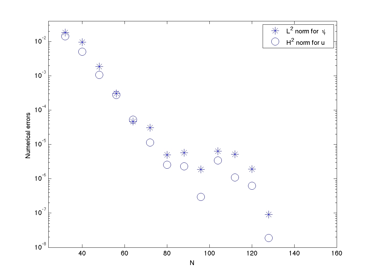
Figure 1: Discrete $L^{2}$ numerical errors for $\psi=u_{t}$ and $H^{2}$ numerical errors for $u$ at $T=4.0$, plotted versus $N$, the number of spatial grid point, for the fully discrete pseudospectral scheme (2.11). The time step size is fixed as $\Delta t=10^{-4}$. An apparent spatial spectral accuracy is observed for both variables.

5.2 Second order convergence in time

To explore the temporal accuracy, we fix the spatial resolution as $N=512$ so that the numerical error is dominated by the temporal ones. We compute solutions with a sequence of time step sizes, $\Delta t=\frac{T}{N_{K}}$, with $N_{K}=100$ to $N_{K}=1000$ in increments of 100, and $T=4$. Fig. 2 shows the discrete $L^{2}$ and $H^{2}$ norms of the errors between the numerical and exact solutions, for $\psi=u_{t}$ and $u$, respectively. A clear second order accuracy is observed for both variables.

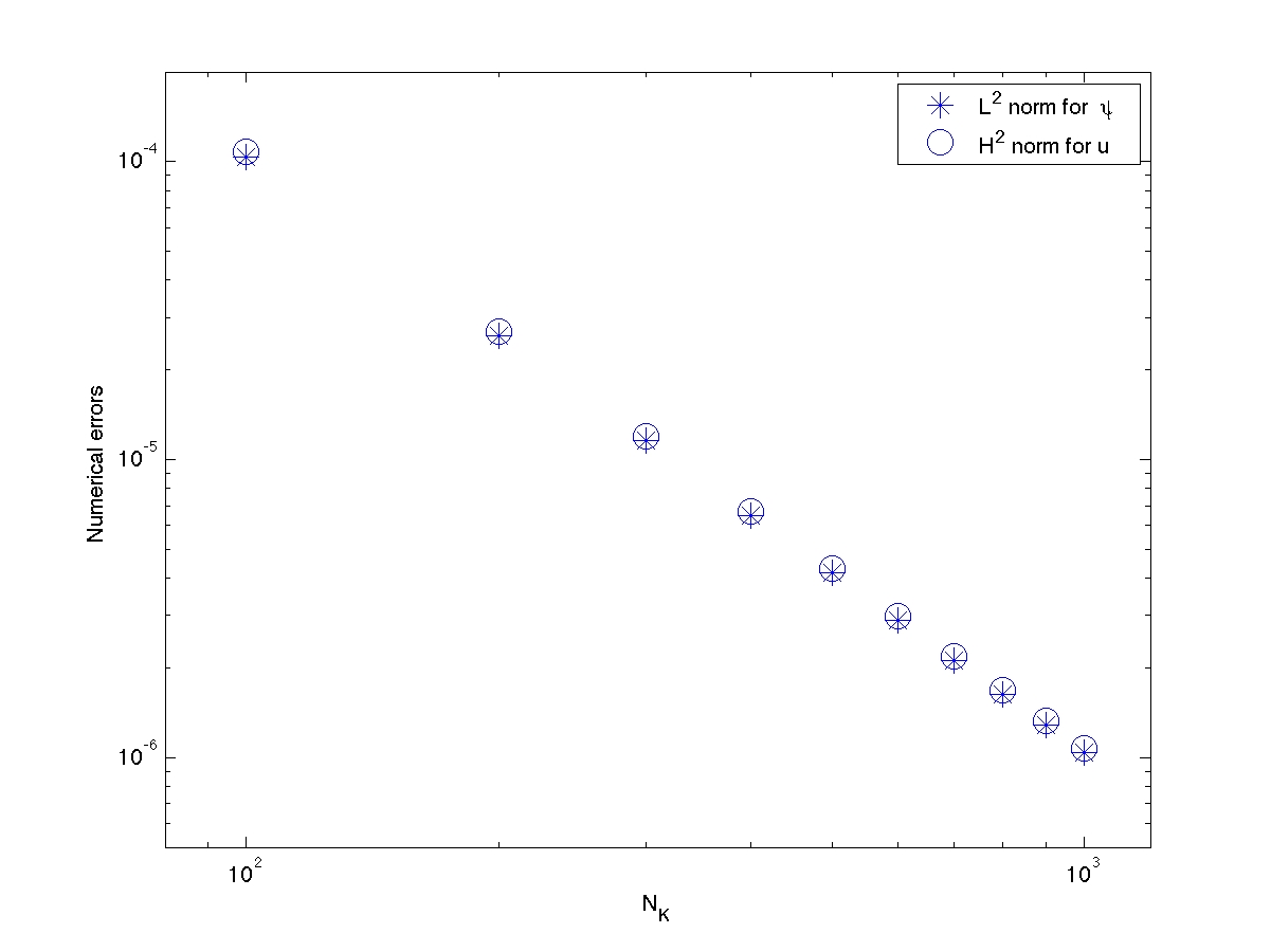
Figure 2: Discrete $L^{2}$ numerical errors for $\psi=u_{t}$ and $H^{2}$ numerical errors for $u$ at $T=4.0$, plotted versus $N_{K}$, the number of time steps, for the fully discrete pseudospectral scheme (2.11). The spatial resolution is fixed as $N=512$. The data lie roughly on curves $CN_{K}^{-2}$, for appropriate choices of $C$, confirming the full second-order temporal accuracy of the proposed scheme.

6 Conclusion Remarks

In this article, we propose a fully discrete Fourier pseudospectral scheme for the GB equation (1.1) with second order temporal accuracy. The nonlinear stability and convergence analysis are provided in detail. In particular, with the help of an aliasing error control estimate (given by Lem. 2.1), an $\ell^{\infty}(0,T^{*};H^{2})$ error estimate for $u$ and $\ell^{\infty}(0,T^{*};\ell^{2})$ error estimate for $\psi=u_{t}$ are derived. Moreover, an introduction of an intermediate variable $\psi$ greatly improves the numerical stability condition; an unconditional convergence (for the time step $\Delta t$ in terms of the spatial grid size $h$) is established in this article, compared with a severe time step constraint $\Delta t\leq Ch^{2}$, reported in an earlier literature [17]. A simple numerical experiment also verifies this unconditional convergence, second order accurate in time and spectrally accurate in space.

References

- [1] B. S. Attili, The Adomian decomposition method for solving the Boussinesq equation arising in water wave propagation, Numer. Methods Partial Differential Equations, 22, 1337-1347, 2006.
- [2] A. Baskara, J S. Lowengrub, C. Wang and S M. Wise, Convergence analysis of a second order convex splitting scheme for the modified phase field crystal equation, SIAM J. Numer. Anal., 51, 2851-2873, 2013.
- [3] J. Boyd, Chebyshev and Fourier Spectral Methods, 2nd edition, Dover, New York, NY, 2001.
- [4] A. G. Bratsos, A predictor-corrector scheme for the improved Boussinesq equation, Chaos, Solitons & Fractals, 40, 2083-2094, 2009.
- [5] A. G. Bratsos, A second order numerical scheme for the improved Boussinesq equation, Physics Letters A, 370, 145-147, 2007.
- [6] A. Bressan and A. Quarteroni, An implicit/explicit spectral method for Burgers’ equation, CALCOLO, 23 (3), 265-284, 1986.
- [7] C. Canuto, M.Y. Hussani, A. Quarteroni and T.A. Zang, Spectral Methods: Evolution to Complex Geometries and Applications to Fluid Dynamics, Springer-Verlag, 2007.
- [8] C. Canuto and A. Quarteroni, Approximation results for orthogonal polynomials in Sobolev spaces, Math. Comp., 38, 67-86, 1982.
- [9] G.Q. Chen, Q. Du and E. Tadmor, Super viscosity approximations to multi-dimensional scalar conservation laws, Math. Comp., 61 (204), 629-643, 1993.
- [10] R. Cienfuegos, E. Barthélemy and P. Bonneton, A fourth-order compact finite volume scheme for fully nonlinear and weakly dispersive Boussinesq-type equations. Part I: Model development and analysis, Int. J. Numer. Methods Fluids, 51, 1217-1253, 2006.
- [11] R. Cienfuegos, E. Barthélemy and P. Bonneton, A fourth-order compact finite volume scheme for fully nonlinear and weakly dispersive Boussinesq-type equations. Part II: Boundary conditions and validation, Int. J. Numer. Methods Fluids, 53, 1423-1455, 2007.
- [12] Q. Du, B. Guo and J. Shen, Fourier spectral approximation to a dissipative system modeling the flow of liquid crystals, SIAM J. Numer. Anal., 39 (3), 735-762, 2001.
- [13] W. E, Convergence of spectral methods for the Burgers’ equation, SIAM J. Numer. Anal., 29 (6), 1520-1541, 1992.
- [14] W. E, Convergence of Fourier methods for Navier-Stokes equations, SIAM J. Numer. Anal., 30 (3), 650-674, 1993.
- [15] H. El-Zoheiry, Numerical investigation for the solitary waves interaction of the “good” Boussinesq equation, Applied Numerical Mathematics, 45, 161-173, 2003.
- [16] L. Farah and M. Scialom, On the periodic “good” Boussinesq equation, Proc. Amer. Math. Soc., 138 (3), 953-964, 2010.
- [17] J. De Frutos, T. Ortega and J. M. Sanz-Serna, Pseudospectiral method for the “good” Boussinesq equation, Math. Comp., 57, 109-122, 1991.
- [18] D. Gottlieb and S.A. Orszag, Numerical Analysis of Spectral Methods, Theory and Applications, SIAM, Philadelphia, PA, 1977.
- [19] S. Gottlieb and C. Wang, Stability and convergence analysis of fully discrete Fourier collocation spectral method for 3-D viscous Burgers’ Equation, Journal of Scientific Computing, 53, 102-128, 2012.
- [20] B.Y. Guo, A spectral method for the vorticity equation on the surface, Math. Comp., 64 (211), 1067-1069, 1995.
- [21] B.Y. Guo and W. Huang, Mixed Jacobi-spherical harmonic spectral method for Navier–Stokes equations, Appl. Numer. Math., 57 (8), 939-961, 2007.
- [22] B.Y. Guo, J. Li and H.P. Ma, Fourier-Chebyshev spectral method for solving three-dimensional vorticity equation, Acta Mathematicae Applicatae Sinica, 11 (1), 94-109, 1995.
- [23] B.Y. Guo, H.P. Ma and E. Tadmor, Spectral vanishing viscosity method for nonlinear conservation laws, SIAM J. Numer. Anal., 39, 1254-1268, 2001.
- [24] B.Y. Guo and J. Shen, On spectral approximations using modified Legendre rational functions: application to the Korteweg-de Vries equation on the half line, Indiana Univ. Math. J., 50, Special issue: Dedicated to Professors Ciprian Foias and Roger Temam, 181-204, 2001.
- [25] B.Y. Guo and J. Zou, Fourier spectral projection method and nonlinear convergence analysis for Navier-Stokes equations, J. Math. Anal. Appl., 282 (2), 766-791, 2003.
- [26] J. Hesthaven, S. Gottlieb and D. Gottlieb, Spectral Methods for Time-Dependent Problems, Cambridge University Press, Cambridge, 2007.
- [27] Q. Lin, Y. H. Wu, R. Loxton and S. Lai, Linear B-spline finite element method for the improved Boussinesq equation, Journal of Computational and Applied Mathematics, 224, 658-667, 2009.
- [28] F. L. Liu and D. L. Russell, Solutions of the Boussinesq equation on a periodic domain, J. Math. Anal. Appl., 192, 194-219, 1995.
- [29] Felipe Linares and Marcia Scialom, Asymptotic behavior of solutions of a generalized Boussinesq type equation, Nonlinear Analysis Theorey, Methods & Applications, 25 (11), 1147-1158, 1995.
- [30] J.C. López-Marcos and J.M. Sanz-Serna, Stability and convergence in numerical analysis. III: Linear investigation of nonlinear stability, IMA J. Numer. Anal., 7, 71-84, 1988.
- [31] Y. Maday, S.M. Ould Kaber and E. Tadmor, Legendre pseudospectral viscosity method for nonlinear conservation laws, SIAM J. Numer. Anal., 30 (2), 321-342, 1993.
- [32] Y. Maday and A. Quarteroni, Legendre and Chebyshev spectral approximations of Burgers’ equation, Numer. Math., 37, 321-332, 1981.
- [33] Y. Maday and A. Quarteroni, Approximation of Burgers’ equation by pseudospectral methods, RAIRO Anal. Numer., 16, 375-404, 1982.
- [34] Y. Maday and A. Quarteroni, Spectral and pseudospectral approximation to Navier-Stokes equations, SIAM J. Numer. Anal., 19 (4), 761-780, 1982.
- [35] A. Majda, J. McDonough and S. Osher, The Fourier method for non-smooth initial data, Math. Comp., 32, 1041-1081, 1978.
- [36] V. S. Manotanjan, A. R. Mitchell and J. L. Morris, Numerical solutions of the good Boussinesq equation, SIAM Sci. Statist. Comp, 5, 946-957, 1984.
- [37] V. S. Manotanjan, T. Ortega and J. M. Sanz-Serna, Soliton and antisoliton interactions in the “good” Boussinesq equation, J. Math. Phy., 29, 1964-1968, 1988.
- [38] S. Oh and A. Stefanov, Improved local well-posedness for the periodic “good” Boussinesq equation, J. Diff. Equ., 254 (10), 4047-4065, 2013.
- [39] T. Ortega and J. M. Sanz-Serna, Nonlinear stability and convergence of finite difference methods for the “good” Boussinesq equation, Numer. Math., 58, 215-229, 1990.
- [40] A. K. Pani and H. Saranga, Finite element Galerkin method for the “good” Boussinesq equation, Non. Anal., 29, 937-956, 1997.
- [41] A. Shokri and M. Dehghan, A Not-a-Knot meshless method using radial basis functions and predictor-corrector scheme to the numerical solution of improved Boussinesq equation, Comput. Phys. Comm., 181, 1990-2000, 2010.
- [42] E. Tadmor, The exponential accuracy of Fourier and Chebyshev differencing methods, SIAM J. Numer. Anal., 23, 1-10, 1986.
- [43] E. Tadmor, Convergence of spectral methods to nonlinear conservation laws, SIAM J. Numer. Anal., 26 (1), 30-44, 1989.
- [44] E. Tadmor, Shock capturing by the spectral viscosity method, Comput. Methods Appl. Mech. Engrg., 80, 197-208, 1990.
- [45] E. Tadmor, Total variation and error estimates for spectral viscosity approximations, Math. Comp., 60 (201), 245-256, 1993.
- [46] E. Tadmor, Burgers’ equation with vanishing hyper-viscosity, Comm. Math. Sci., 2 (2), 317-324, 2004.
- [47] M. Tsutsumi and T. Matahashi, On the Cauchy problem for the Boussinesq type equation, Math. Japan, 36 (2), 371-379, 1991.
- [48] C. Wang and S. Wise, An energy stable and convergent finite-difference scheme for the modified phase field crystal equation, SIAM J. Numer. Anal., 49, 945-969, 2011.
- [49] A. M. Wazwaz, Constructions of soliton solutions and periodic solutions of the Boussinesq equation by the modified decomposition method, Chaos Solitons & Fractals, 12, 1549-1556, 2001.
- [50] R. Xue, The initial-boundary value problem for the “good” Boussinesq equation on the bounded domain, J. Math. Anal. Appl., 343, 975-995, 2008.