NLO corrections to $\chi_{bJ}$ to two-$J/\psi$ exclusive decay processes

Abstract

The next-to-leading order QCD corrections for $\chi_{bJ}$, the p-wave bottomonium, to $J/\psi$ pair decay processes are evaluated utilizing NRQCD factorization formalism. The scale dependence of $\chi_{b2}\rightarrow J/\psi J/\psi$ process is depressed with NLO corrections, and hence the uncertainties in the leading order results are greatly reduced. The total branch ratios are found to be the order of $10^{-5}$ for all three $\chi_{bJ}\rightarrow J/\psi J/\psi$ processes, indicating that they are observable in the LHC and super-B experiments.

PACS number(s): 12.38.Bx, 13.25.Gv, 14.40.Be

I Introduction

The advent of non-relativistic Quantum Chromodynamics (NRQCD) factorization formalism causes investigations on heavy quarkonium more reliable NRQCD , which improves the understanding of strong interaction. It has been noted that for quarkonium production and decay, in many cases the leading order calculation in the framework of NRQCD is inadequate. The discrepancies between leading order calculations and experimental results are rectified by including higher order corrections, which has encouraged various investigations. One typical example is the double charmonium production in B-factory belle ; bralee ; hqiao ; lhch ; ZYJ ; GB1 . Furthermore, corrections of higher order in the heavy-quark velocity $v$ are also important in obtaining reliable predictions for quarkonium exclusive decays fengjias ; dfjia ; lmchao .

Inspired by the theoretical description of the double charmonium production in B-factory, the bottomonium to double charmonium decay processes have also been broadly investigated. As in bottomonium to $J/\psi$ pair exclusive decay processes the color-octet contribution is negligible, the theoretical evaluation result is quite explicit in comparison with the experimental data. The decays of $\eta_{b}$ to double $J/\psi$ Jia ; GB2 ; Bra ; SP , $\Upsilon$ to $J/\psi+\chi_{cJ}$ jdf , and $\chi_{bJ}$ to double $J/\psi$ FF ; SWL ; qiao had been thoroughly investigated. The process $\chi_{bJ}\rightarrow J/\psi J/\psi(J=0,2)$ was evaluated in the frameworks of NRQCD and light cone distribution amplitude at the leading order in $\alpha_{s}$ expansion, except $\chi_{b1}\rightarrow J/\psi J/\psi$ process. In order to make the prediction more accurate and reduce the renormalization scale dependence, it is essential to evaluate the process with the NLO QCD corrections. In this aim, we calculate in the work the Next-to-Leading order(NLO) QCD corrections to the P-wave bottomonium $\chi_{bJ}$ decays to double $J/\psi$ in the framework of NRQCD. We obtain the completely analytical results for these three $\chi_{bJ}\rightarrow J/\psi J/\psi$ one loop processes.

The rest of this paper is organized as follows. Section II presents the strategy and formalism for the study of $\chi_{bJ}\rightarrow J/\psi J/\psi$ processes. Section III comprises numerical calculation and discussion on the results. Section IV gives a summary and some conclusions. Several formulas are provided in the Appendix for reference.

II Calculation Scheme Description and Formalism

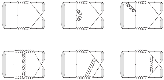
Figure 1: Typical Feynman diagrams for $\chi_{bJ}\rightarrow J/\psi J/\psi$ decays.

In the calculation, we use Mathematica package FeynArts feynarts to generate all the Feynman diagrams and decay amplitudes. Certain typical representative diagrams are shown in Fig.1. All the projection operators for quarkonium in this work may be found in Ref.bodwpe ; braaten . For the spin-triplet color-singlet state, the matrix product is expressed as:

$$v(\bar{p})\bar{u}(p)=\frac{1}{4\sqrt{2}E(E+m)}(\not\!\bar{p}-m_{c})\not\!\epsilon_{S}^{*}(\not\!P+2E)(\not\!p+m_{c})\otimes\bigg{(}\frac{\bf{1}_{c}}{\sqrt{N_{c}}}\bigg{)}\ .$$ (1)

Here $p=\frac{P}{2}+q,~{}\bar{p}=\frac{P}{2}-q$ respectively are the momenta of quark and antiquark, $\not\!\epsilon^{*}$ is a spin polarization vector, $E^{2}=P^{2}/4=m_{c}^{2}-q^{2}$, $N_{c}=3$, and $\bf{1}_{c}$ represents the unit color matrix. For the spin-singlet and color-singlet state, the projection operator may be obtained by replacing the $\epsilon_{S}^{*}$ in (1) with a $\gamma_{5}$.

Using the method described in braaten and applying FeynCalc Feyncalc to the calculation of amplitudes, the tree-level results are readily obtained. For One-loop QCD corrections, more operations are necessary before arriving at the final result. For $\chi_{b0}$ and $\chi_{b2}$ decays to the double $J/\psi$ processes, there are 2 tree-level diagrams, 76 one-loop diagrams and 14 counter terms. While for the $\chi_{b1}\rightarrow J/\psi J/\psi$ process, the contribution of gluon self-energy, triangle and four box diagrams vanish, and there are only 44 one-loop diagrams functioning. The ultra divergences are proportional to tree level amplitudes, hence they vanish for $\chi_{b1}\rightarrow J/\psi J/\psi$ process and hence no counter term is necessary.

In the calculation, Feynman diagrams and amplitudes are generated by FeynArts. FeynCalc is used to trace the matrices of spin and color, and to perform the derivation on the heavy quark relative momentum $q$ within quarkonium. The Mathematica package Apart apart reduces the propagator of each individual one-loop diagram. The package Fire fire is employed to reduce all one-loop integrals to typical master-integrals. The calculation is performed in the Feynman gauge, while the Conventional dimensional regularization with $D=4-2\epsilon$ is adopted in regularizing the divergences. In the end, ultraviolet divergences are completely canceled by counterterms, the Coulomb singularities are factored and attribute to the NRQCD long-distance matrix elements, and those infra divergences of short-distance coefficients cancel with each other, which confirms the NRQCD factorization for these processes at the NLO order.

In the expansion of strong coupling constant $\alpha_{s}$, decay width is formally expressed as:

$$d\Gamma\propto|\mathcal{M}_{tree}+\mathcal{M}_{oneloop}+\cdots|^{2}=|\mathcal{M}_{tree}|^{2}+2Re(\mathcal{M}_{tree}^{*}\mathcal{M}_{oneloop})+|\mathcal{M}_{oneloop}|^{2}+\cdots\ .$$

For $\chi_{b0,2}\rightarrow J/\psi J/\psi$ processes, up to the one-loop level, one only needs to keep the the first and second terms. For $\chi_{b1}\rightarrow J/\psi J/\psi$ process, the tree level amplitude does not exist, and hence the leading order contribution comes from the one-loop amplitudes. By virtue of parity and Lorentz invariance, the decay amplitude for $\chi_{b1}\rightarrow J/\psi J/\psi$ can be constructed as following tensor structure:

$$\mathcal{M}(\lambda,\lambda_{1},\lambda_{2})=(\varepsilon_{\mu\rho_{1}\rho_{2}\sigma}P_{\psi_{1}}^{\nu}-\varepsilon_{\nu\rho_{1}\rho_{2}\sigma}P_{\psi_{2}}^{\mu})\epsilon_{\psi_{1}}^{\mu}\epsilon_{\psi_{2}}^{\nu}P_{\psi_{1}}^{\rho_{1}}P_{\psi_{2}}^{\rho_{2}}\epsilon_{\chi_{b}}^{\sigma}\mathcal{A}\ ,$$ (2)

where $P_{\psi_{1}}$ and $P_{\psi_{2}}$ are the momenta of two final $J/\psi$s, $\epsilon$ denotes the polarization vector, and $\mathcal{A}$ is a scalar function of $m_{b}$ and $m_{c}$.

The ultraviolet and infrared divergences are contained in the renormalization constants $Z_{2},Z_{3},Z_{m},Z_{g}$, correspond respectively to the quark field, gluon field, quark mass, and strong coupling constant $\alpha_{s}$. Among them, in our calculation the $Z_{g}$ and $Z_{3}$ are defined in the modified-minimal-subtraction $\overline{MS}$ scheme, while others are in the on-shell (OS) scheme. Thereafter, the counter terms read:

$$\delta Z_{2}^{\rm OS} = -C_{F}\frac{\alpha_{s}}{4\pi}\left[\frac{1}{\epsilon_{\rm UV}}+\frac{2}{\epsilon_{\rm IR}}-3\gamma_{E}+3\ln\frac{4\pi\mu^{2}}{m^{2}}+4\right],$$

$$\delta Z_{m}^{\rm OS} = -3C_{F}\frac{\alpha_{s}}{4\pi}\left[\frac{1}{\epsilon_{\rm UV}}-\gamma_{E}+\ln\frac{4\pi\mu^{2}}{m^{2}}+\frac{4}{3}\right],$$

$$\delta Z_{3}^{\overline{\rm MS}} = \frac{\alpha_{s}}{4\pi}(\bar{\beta}_{0}-2C_{A})\left[\frac{1}{\epsilon_{\rm UV}}-\gamma_{E}+\ln(4\pi)\right],$$

$$\delta Z_{g}^{\overline{\rm MS}} = -\frac{\bar{\beta}_{0}}{2}\,\frac{\alpha_{s}}{4\pi}\left[\frac{1}{\epsilon_{\rm UV}}-\gamma_{E}+\ln(4\pi)\right].$$ (3)

Note that since the tree level contribution for $\chi_{b1}\rightarrow J/\psi J/\psi$ vanishes, the infrared divergences of short-distance coefficients appearing in the one-loop diagrams cancel with each other, and no ultraviolet divergences appear, this process is naturally finite in the next-to-leading order. The analytical results for the $\chi_{bJ}\rightarrow J/\psi J/\psi$ decay widths up to the one-loop level are given in the Appendix for reference.

III Results and discussion

III.1 Input parameters

Before carrying out numerical calculation, the input parameters need to be fixed. For the NRQCD matrix elements, those from Refs. qiao ; chao , i.e. $\langle\mathcal{O}_{1}\rangle_{\chi_{bJ}}=2.03\ \textrm{GeV}^{5}$ and $\langle\mathcal{O}_{1}\rangle_{J/\psi}=\frac{27m_{c}^{2}\Gamma(J/\psi\rightarrow e^{+}e^{-})}{8\pi\alpha^{2}(1-4C_{F}\alpha_{s}/\pi)}=0.20\ \textrm{GeV}m_{c}^{2}$, are utilized. The charm quark and bottom quark masses are taken to be $m_{c}=1.5\pm 0.1$ GeV and $m_{b}=4.9\pm 0.1$ GeV respectively. The masses of quarkonia are obtained from the PDG PDG , which read $M_{\chi_{b0}}=9.859$ GeV, $M_{\chi_{b1}}=9.892$ GeV, $M_{\chi_{b2}}=9.912$ GeV, $M_{J/\psi}=3.097$ GeV. The two-loop expression for the running coupling constant $\alpha_{s}^{l}(\mu)$ with $n_{l}$ the number of light active flavors reads

$$\frac{\alpha_{s}^{n_{l}}(\mu)}{4\pi}=\frac{1}{\beta_{0}L}-\frac{\beta_{1}\ln L}{\beta_{0}^{3}L^{2}}\ .$$ (4)

Here, $L=\ln(\mu^{2}/\Lambda_{QCD}^{2})$, $\beta_{0}=(11/3)C_{A}-(4/3)T_{F}n_{l}$, and $\beta_{1}=(34/3)C_{A}^{2}-4C_{F}T_{F}n_{l}-(20/3)C_{A}T_{F}n_{l}$, with $\Lambda_{QCD}$ to be $339$ MeV and $n_{l}=3$, the number of light active flavors $(m_{q}\ll\mu)$. For numerical calculation in this work, the renormalization scale is about the order of $m_{c}$, and the strong coupling constant involves four active flavors, three light flavors and a massive flavor, the charm quark. Using a matching relation one may transit a running in terms of three active light flavors to a running in terms of four active flavors PDG , i.e.,

$$\alpha_{s}^{n_{l}+1}(\mu)=\alpha_{s}^{n_{l}}(\mu)\bigg{(}1+\sum_{n=1}^{\infty}\sum_{i=0}^{n}c_{ni}[\alpha_{s}^{n_{l}}(\mu)]^{n}\ln^{i}(\frac{\mu^{2}}{m_{c}^{2}})\bigg{)}\ .$$ (5)

We take the two loop results for this expansion with the coefficients $c_{ni}$ are $c_{11}=\frac{1}{6\pi},c_{10}=0,c_{22}=c_{11}^{2},c_{21}=\frac{19}{24\pi^{2}}$, and $c_{20}=\frac{7}{24\pi^{2}}$ when $m_{c}$ is the pole mass. The $\alpha_{s}^{l+1}(\mu)$ is adopted in our numerical calculation and the $\bar{\beta}_{0}$ in counter terms $\{\delta Z_{3},\delta Z_{g}\}$ is expressed as $\bar{\beta}_{0}=(11/3)C_{A}-(4/3)T_{F}n_{f}$ with $n_{f}=3+1$.

III.2 Results and Discussion

After substituting the input parameters in the preceding subsection to the analytical expressions, the numerical results are readily obtained. The magnitudes of the decay widths for $\chi_{bJ}\rightarrow J/\psi J/\psi$ are presented in Table I, where the first uncertainty comes from $m_{b}$ and the second one from the $m_{c}$. With the relation $\langle\mathcal{O}_{1}\rangle_{J/\psi}=0.20\ \textrm{GeV}m_{c}^{2}$, the uncertainty of charmonium matrix element is attributed to that of $m_{c}$. In numerical evaluation, we let renormalization scale $\mu$ run from $m_{b}$ and $2m_{b}$ to estimate the uncertainties induced by even higher order contributions.

Table 1: Decay widths for $\chi_{bJ}\rightarrow J/\psi J/\psi$ at leading order and next-to-leading order, all in units of eV, with $m_{b}=4.9\pm 0.1$ GeV, $m_{c}=1.5\pm 0.1$ GeV, and $\mu\in\{m_{b},2m_{b}\}$.

$\Gamma$(eV)	LO$\chi_{b0}$	NLO$\chi_{b0}$	LO$\chi_{b2}$	NLO$\chi_{b2}$	$\textrm{LO}\chi_{b1}$
$\mu=m_{b}$	$7.66^{+1.33+0.75}_{-1.12-0.73}$	$13.13^{+2.32+1.24}_{-1.93-1.18}$	$19.54^{+3.94+3.55}_{-3.21-3.11}$	$12.85^{+2.47+2.11}_{-2.03-1.90}$	$0.58^{+0.09+0.01}_{-0.08-0.01}$
$\mu=2m_{b}$	$3.56^{+0.59+0.35}_{-0.51-0.34}$	$7.85^{+1.34+0.76}_{-1.12-0.73}$	$9.07^{+1.78+1.66}_{-1.45-1.45}$	$12.11^{+2.35+2.12}_{-1.93-1.88}$	$0.18^{+0.03+0.00}_{-0.02-0.00}$

(a) $\chi_{b0}\rightarrow J/\psi J/\psi$

(b) $\chi_{b2}\rightarrow J/\psi J/\psi$

Figure 2: The scale $\mu$ dependence for $\chi_{bJ}\rightarrow J/\psi J/\psi(J=0,2)$ decay widths at LO and NLO. Here $m_{b}=4.9\ \textrm{GeV},m_{c}=1.5\ \textrm{GeV},\textrm{and}\ \Lambda_{QCD}=339\ \textrm{MeV}$.

In Figure 2 we show the renormalization scale dependence of the leading order and the next-to-leading order decay widths of $\chi_{b0,2}\rightarrow J/\psi J/\psi$ processes. For these two processes, the decay widths are proportional to $\alpha_{s}^{4}(\mu)$ at the Born level, therefore having strong scale dependence. Fig. 2 exhibits that the $\mu$ dependence for $\chi_{b0}\rightarrow J/\psi J/\psi$ is still evident with the NLO QCD corrections, while for $\chi_{b2}\rightarrow J/\psi J/\psi$ the $\mu$ dependence is substantially suppressed by the NLO QCD corrections. Note that for $\chi_{b1}\rightarrow J/\psi J/\psi$ process, since the tree diagrams make null contribution, the effective leading order diagrams are at the one-loop level. So, in this work only the leading order results are provided for the $\chi_{b1}\rightarrow J/\psi J/\psi$ decay process. Because the decay width of this process is proportional to $\alpha_{s}^{6}(\mu)$, the $\mu$ dependence is prominent in comparison with the other two processes. The decay width alters from 0.18 eV to 0.58 eV when the renormalization scale $\mu$ varying from $m_{b}$ to $2m_{b}$.

Table 2: Decay widths and branching ratios of $\chi_{bJ}\to J/\psi J/\psi$. The first and second rows are the NLO results of this work with scale $\mu=m_{b}$. The third and fourth rows are the leading order results obtained in Refs. FF ; SWL with relativistic corrections. The last row shows the branching ratio upper limits set by the Belle experiment belle1 .

	$\chi_{b0}\to J/\psi J/\psi$	$\chi_{b1}\to J/\psi J/\psi$	$\chi_{b2}\to J/\psi J/\psi$
$\Gamma^{\text{NLO}}$(eV)	$13.13^{+2.32+1.24+2.10}_{-1.93-1.18-5.39}$	$0.58^{+0.09+0.01+0.28}_{-0.12-0.01-0.40}$	$12.85^{+2.47+2.11+0.70}_{-2.03-1.90-2.66}$
Br${}^{\text{NLO}}$($10^{-5}$)	$1.80^{+0.32+0.17+0.29}_{-0.26-0.16-0.74}$	$0.63^{+0.10+0.01+0.30}_{-0.13-0.01-0.43}$	$5.85^{+1.12+0.96+0.32}_{-0.92-0.86-1.21}$
$\Gamma^{\text{LO}}$(eV) FF	5.54	$9.04\times 10^{-7}$	10.6
$\Gamma^{\text{LO}}$(eV) SWL	15	$3.1\times 10^{-4}$	35
Br${}^{\text{EXP}}$($10^{-5}$) belle1	$<$7.1	$<$2.7	$<$4.5

In Table II the theoretical predictions and experiment measurements for processes of p-wave bottomnium decays to $J/\psi$ pairs are given. Of our calculation, the next-to-leading order ones, there exist three main sources of uncertainties, i.e. from the uncertainties in charm quark mass, bottom quark mass and the variation of renormalization scale. Note that in practice the uncertainty in quarkonium non-perturbative matrix element also has a big effect in the calculation, whereas this effect is attributed to the charm quark mass through relation $\langle\mathcal{O}_{1}\rangle_{J/\psi}=0.20\textrm{GeV}m_{c}^{2}$ in our investigation as mentioned in above.

Once the Belle Collaboration had measured the $\chi_{bJ}\to J/\psi J/\psi$ processes and obtained the corresponding upper limits for branching ratios at the $90\%$ confidence level belle1 , which, as shown in the Table II, are compatible with our estimations, i.e. at the order of $10^{-5}$. Though no significant signals for $\chi_{bJ}\to J/\psi J/\psi$ have yet been observed at the B-factory, from our calculation, they might be observed at the LHC or future Super-B factory. According to Ref. bra , while $\sqrt{s}=14\text{TeV}$ the production cross sections of $\chi_{b0}$ and $\chi_{b2}$ at the LHC with are $\sigma(pp\rightarrow\chi_{b0}+X)=1.5\mu b$ and $\sigma(pp\rightarrow\chi_{b2}+X)=2\mu b$, respectively. In 2012, the luminosity of LHC was about $50\text{fb}^{-1}$, so about $7.5\times 10^{10}\chi_{b0}$ and $10^{11}\chi_{b2}$ were produced per year even at such luminosity. This means that approximately thousands of $\chi_{b0,2}\rightarrow J/\psi J/\psi\rightarrow l^{+}l^{-}l^{+}l^{-}$($l=e\ or\ \mu$) processes happen each year at the LHC. As an example, the LHCb detector covers a range of pseudo-rapidity $2<\eta<5$, and for the dimuon event it requires the transverse momenta of the produced muon pair satisfying $\sqrt{p_{T1}p_{T2}}>1.3$ GeV lhcb . Obviously, most of the events of the concerned processes satisfy this requirement, hence the high detection efficency and the substantial possibility of measuring the $\chi_{bJ}\rightarrow J/\psi J/\psi$ processes at the LHC.

IV Summary and Conclusions

This work features a complete one-loop calculation for $\chi_{bJ}\to J/\psi J/\psi$ exclusive decays in the framework of NRQCD factorization. All infra divergences of short-distance coefficients are canceled out and hence confirms the NRQCD factorization in these processes at the next-to-leading order. Taking $m_{b}=4.9\ \textrm{GeV},m_{c}=1.5\ \textrm{GeV}$, numerical results show that the NLO QCD corrections for the decay width of $\chi_{b0}\to J/\psi J/\psi$ are all positive within the energy scale range of $m_{b}$ to $2m_{b}$. While for $\chi_{b2}\to J/\psi J/\psi$, the NLO correction is negative at scale $\mu=m_{b}$ and positive at scale $\mu=2m_{b}$. As for $\chi_{b1}\to J/\psi J/\psi$ decay, the leading order process is at the one-loop level, which yields a notable number of events. Calculation results indicate that the renormalization scale $\mu$ dependence for $\chi_{b0}\to J/\psi J/\psi$ remains to be distinct with the NLO correction, while for $\chi_{b2}\to J/\psi J/\psi$ the $\mu$ dependence is substantially reduced. The branching ratios of all three $\chi_{bJ}\to J/\psi J/\psi$ decay processes are of the order $10^{-5}$. Although no evident signal has been observed in the B-factory, with more high-luminosity and statistics, these p-wave bottomnium to double $J/\psi$ exclusive decay processes may be observed at the LHC or future Super-B experiment.

Acknowledgments

This work was supported in part by the National Natural Science Foundation of China(NSFC) under the grant Nos. 10935012, 11121092, 11175249 and 11375200.

Appendix A amplitude

The analytical results of the calculation are as follows. For the sake of simplicity of the expressions, we denote $a=\frac{m_{c}^{2}}{m_{b}^{2}}$. The leading order decay widths for $\chi_{b0,2}\to J/\psi J/\psi$ are formulated as:

$$\Gamma_{\chi_{bJ}}^{LO}(J=0,2)=\frac{\pi^{3}\alpha^{4}_{s}(\mu)\langle\mathcal{O}_{1}\rangle_{\chi_{bJ}}\langle\mathcal{O}_{1}\rangle^{2}_{J/\psi}\mathbb{M}^{J}_{LO}}{(2J+1)373248m_{b}^{7}m_{c}^{2}M_{\chi_{bJ}}}\sqrt{1-\frac{4M^{2}_{J/\psi}}{M^{2}_{\chi_{bJ}}}}$$ (6)

with $\mathbb{M}^{0}_{LO}=1048576(1-4a+12a^{2})/3$ and $\mathbb{M}^{2}_{LO}=524288(13+56a+48a^{2})/3$ for $\chi_{b0,b2}\to J/\psi J/\psi$ processes, and

$$\Gamma_{\chi_{b1}}^{LO}=\frac{\pi\alpha^{6}_{s}(\mu)\langle\mathcal{O}_{1}\rangle_{\chi_{b1}}\langle\mathcal{O}_{1}\rangle^{2}_{J/\psi}|\mathbb{M}^{1}_{LO}|^{2}}{34992m_{b}^{11}M_{\chi_{b1}}(m_{b}^{2}-4m_{c}^{2})^{2}}\sqrt{1-\frac{4M^{2}_{J/\psi}}{M^{2}_{\chi_{b1}}}}$$ (7)

for $\chi_{b1}\to J/\psi J/\psi$ process. Here,

$$\mathbb{M}^{1}_{LO} =32m_{b}(42+212a-1421a^{2}+504a^{3})A_{0}(1)/(21a^{2})+16m_{b}(-84+27a$$

$$+4464a^{2}+712a^{3})A_{0}(2)/(21a^{2})-16m_{b}^{3}(3515-1352a)B_{0}(1)/21$$

$$+32m_{b}^{3}(1-28a-104a^{2})B_{0}(2)/(3a)-1728m_{b}^{3}(1-4a)B_{0}(4)/7$$

$$+32m_{b}^{3}(1-7a+8a^{2})B_{0}(5)/(3a)+16m_{b}^{3}(84-111a-349a^{2}$$

$$+2940a^{3})B_{0}(6)/(21a^{2})-32m_{b}^{3}(2+15a+151a^{2}+72a^{3})B_{0}(7)/(3a)$$

$$+864m_{b}^{5}C_{0}(1)(1-4a)/7-32m_{b}^{5}C_{0}(2)(3+10a)/3-64m_{b}^{5}C_{0}(3)(7$$

$$+72a)/3-16m_{b}^{5}(815-126a-112a^{2})C_{0}(4)/21-32m_{b}^{5}C_{0}(5)(7-2a)/3$$

$$+16m_{b}^{5}C_{0}(6)(45+288a-16a^{2})/3-256m_{b}^{5}C_{0}(7)(35+67a)/3$$

$$+512m_{b}^{5}C_{0}(8)a(13-24a)/3-32m_{b}^{5}(21-2365a+2213a^{2}-504a^{3})/(21a)\ .$$

The NLO decay widths are formulated as :

$$\Gamma_{\chi_{bJ}}^{NLO}(J=0,2) = \Gamma_{\chi_{bJ}}^{LO}\bigg{(}1+\frac{16\alpha_{s}(\mu)\textrm{Re}(131072\mathbb{M}^{J}_{NLO})}{\pi m_{b}^{2}\mathbb{M}^{J}_{LO}}\bigg{)}.$$ (9)

Here,

$$\mathbb{M}^{0}_{NLO} =A_{0}(1)(715-8959a+50042a^{2}-142196a^{3}+169032a^{4}+26688a^{5}$$ (10)

$$-150912a^{6})/(27a(1-9a+26a^{2}-24a^{3}))+2A_{0}(2)(46-1015a+6578a^{2}$$

$$-18023a^{3}+17406a^{4}+8688a^{5}-18720a^{6})/(27a(1-9a+26a^{2}-24a^{3}))$$

$$-((16n_{l}-177)-8(8n_{l}-91)a+12(16n_{l}-151)a^{2})m_{b}^{2}B_{0}(1)/9+(2$$

$$+31a-824a^{2}+2172a^{3})m_{b}^{2}B_{0}(2)/(9a)-11(1-4a+12a^{2})m_{b}^{2}B_{0}(3)/3$$

$$+2(11-11a+48a^{2}-180a^{3})m_{b}^{2}B_{0}(4)/(3(1-3a))+2(1-18a+62a^{2}-152a^{3}$$

$$+168a^{4}+864a^{5}-1536a^{6})m_{b}^{2}B_{0}(5)/(9a(1-6a+8a^{2}))-2(46-851a+5040a^{2}$$

$$-11755a^{3}+6560a^{4}+4248a^{5}+17592a^{6}-29664a^{7})m_{b}^{2}B_{0}(6)/(27a(1-9a$$

$$+26a^{2}-24a^{3}))-2(2-11a-326a^{2}+738a^{3}+444a^{4})m_{b}^{2}B_{0}(7)/(9a)$$

$$-6a(11+6a)m_{b}^{4}C_{0}(1)-4a(19-52a+60a^{2})m_{b}^{4}C_{0}(2)/9+8a(130a$$

$$-79)m_{b}^{4}C_{0}(3)/9-2(20-207a+242a^{2}-24a^{3})m_{b}^{4}C_{0}(4)/9-4(1+11a$$

$$+12a^{2}-12a^{3})m_{b}^{4}C_{0}(5)/9-8(15-89a+130a^{2}+54a^{3})m_{b}^{4}C_{0}(6)/9$$

$$+8(4-107a+102a^{2})m_{b}^{4}C_{0}(7)/9+16(5-14a-8a^{2}+48a^{3})m_{b}^{4}C_{0}(8)/9$$

$$+8(1-4a+12a^{2})m_{b}^{2}\ln(\frac{m_{b}^{2}}{\mu^{2}})/3+32(1-4a+12a^{2})m_{b}^{2}\ln(\frac{m_{c}^{2}}{\mu^{2}})/3$$

$$+2(8n_{l}-561+(6693-88n_{l})a+2(208n_{l}-17631)a^{2}+6(15947-176n_{l})a^{3}$$

$$+48(24n_{l}-2383)a^{4}+23904a^{5})m_{b}^{2}/(27(1-7a+12a^{2}))$$

and

$$\mathbb{M}^{2}_{NLO} =2A_{0}(1)(2041-9067a-16630a^{2}+96184a^{3}-7260a^{4}-133848a^{5}$$ (11)

$$-45792a^{6})/(81a(1-9a+26a^{2}-24a^{3}))-4A_{0}(2)(655-3703a+13256a^{2}$$

$$-64022a^{3}+154758a^{4}-38484a^{5}-163728a^{6})/(405a(1-9a+26a^{2}-24a^{3}))$$

$$-((520n_{l}-11097)+2(1120n_{l}-15527)a+48(40n_{l}-379)a^{2})m_{b}^{2}B_{0}(1)/135$$

$$-2(5-201a-4702a^{2}-6096a^{3})m_{b}^{2}B_{0}(2)/(135a)-38(13+56a+48a^{2})m_{b}^{2}B_{0}(3)/45$$

$$+4(212+538a-1635a^{2}-3636a^{3})m_{b}^{2}B_{0}(4)/(45(1-3a))-2(1+75a+142a^{2}+44a^{3}$$

$$-776a^{4}-768a^{5})m_{b}^{2}B_{0}(5)/(27a(1-2a))+(524-1225a-13281a^{2}+48988a^{3}$$

$$-26300a^{4}-7392a^{5}-24768a^{6}-55296a^{7})m_{b}^{2}B_{0}(6)/(81a(1-9a+26a^{2}-24a^{3}))$$

$$+2(2-1187a-2102a^{2}-2040a^{3}-636a^{4})m_{b}^{2}B_{0}(7)/(27a)$$

$$+2(12-a-12a^{2})m_{b}^{4}C_{0}(1)/3+4(3+34a-82a^{2}-84a^{3})m_{b}^{4}C_{0}(2)/27$$

$$-8(3-133a-290a^{2})m_{b}^{4}C_{0}(3)/27-2(4-61a-566a^{2}-360a^{3})m_{b}^{4}C_{0}(4)/27$$

$$+8(2+16a+9a^{2}-6a^{3})m_{b}^{4}C_{0}(5)/27-2(396+1381a+572a^{2}-24a^{3})m_{b}^{4}C_{0}(6)/27$$

$$-4(275-820a+204a^{2})m_{b}^{4}C_{0}(7)/27+16(1+40a+32a^{2}-72a^{3})m_{b}^{4}C_{0}(8)/27$$

$$-8(13+56a+48a^{2})m_{b}^{2}\ln(\frac{m_{b}^{2}}{\mu^{2}})/9+16(13+56a+48a^{2})m_{b}^{2}\ln(\frac{m_{c}^{2}}{\mu^{2}})/9$$

$$+4(130n_{l}-3408-70(5n_{l}+126)a+(140163-1880n_{l})a^{2}+6(560n_{l}-21261)a^{3}$$

$$+18(320n_{l}-21407)a^{4}-11880a^{5})m_{b}^{2}/(405(1-7a+12a^{2}))$$

with

$$x_{1,2}=\frac{1\pm\sqrt{1-4a}}{2}\ ,\ y_{1,2}=\frac{1\pm\sqrt{1-4a}}{2\sqrt{a}}\ ,$$ (12)

$$A_{0}(1)=A_{0}(m_{c}^{2})=m_{c}^{2}(1+\ln(\frac{\mu^{2}}{m_{c}^{2}}))\ ,$$ (13)

$$A_{0}(2)=A_{0}(m_{b}^{2})=m_{b}^{2}(1+\ln(\frac{\mu^{2}}{m_{b}^{2}}))\ ,$$ (14)

$$B_{0}(1)=B_{0}(m_{b}^{2},0,0)=2+\ln(\frac{\mu^{2}}{m_{b}^{2}})+i\pi\ ,$$ (15)

$$B_{0}(2)=B_{0}(4m_{b}^{2},0,0)=2+\ln(\frac{\mu^{2}}{4m_{b}^{2}})+i\pi\ ,$$ (16)

$$B_{0}(3)=B_{0}(m_{b}^{2},0,m_{b}^{2})=2+\ln(\frac{\mu^{2}}{m_{b}^{2}})\ ,$$ (17)

$$B_{0}(4)=B_{0}(m_{b}^{2},m_{b}^{2},m_{b}^{2})=\ln(\frac{\mu^{2}}{m_{b}^{2}})+2-\frac{\pi}{\sqrt{3}}\ ,$$ (18)

$$B_{0}(5)=B_{0}(m_{b}^{2},m_{c}^{2},m_{c}^{2})=2+\ln(\frac{\mu^{2}}{m_{b}^{2}})-\sum_{i=1}^{2}2x_{i}\ln(x_{i})+i\pi\ ,$$ (19)

$$B_{0}(6)=B_{0}(m_{c}^{2},m_{b}^{2},m_{c}^{2})=2+\ln(\frac{\mu^{2}}{m_{c}^{2}})-\sum_{i=1}^{2}(x_{i}\ln(\frac{x_{i}-1}{x_{i}})-\ln(x_{i}-1))\ ,$$ (20)

$$B_{0}(7)=B_{0}(2m_{b}^{2}+m_{c}^{2},0,m_{c}^{2})=2+\ln(\frac{\mu^{2}}{m_{c}^{2}})-\frac{2}{2+a}(\ln(2a)-i\pi)\ ,$$ (21)

$$C_{0}(1)=C_{0}(m_{b}^{2},m_{c}^{2},m_{c}^{2},m_{b}^{2},m_{b}^{2},m_{c}^{2})\ ,$$ (22)

$$C_{0}(2)=C_{0}(m_{b}^{2},m_{c}^{2},2m_{b}^{2}+m_{c}^{2},m_{c}^{2},m_{c}^{2},0)\ ,$$ (23)

$$C_{0}(3)=C_{0}(4m_{b}^{2},m_{c}^{2},2m_{b}^{2}+m_{c}^{2},0,0,m_{c}^{2})\ ,$$ (24)

$$C_{0}(4)=C_{0}(m_{b}^{2},m_{c}^{2},m_{c}^{2},0,0,m_{c}^{2})\ ,$$ (25)

$$C_{0}(5)=C_{0}(m_{b}^{2},m_{c}^{2},m_{c}^{2},m_{c}^{2},m_{c}^{2},m_{b}^{2})\ ,$$ (26)

$$C_{0}(6)=C_{0}(m_{b}^{2},m_{c}^{2},2m_{b}^{2}+m_{c}^{2},0,0,m_{c}^{2})\ ,$$ (27)

$$C_{0}(7)=C_{0}(m_{b}^{2},m_{c}^{2},2m_{b}^{2}+m_{c}^{2},0,m_{b}^{2},m_{c}^{2})\ ,$$ (28)

$$C_{0}(8)=C_{0}(m_{c}^{2},4m_{c}^{2},2m_{b}^{2}+m_{c}^{2},0,m_{c}^{2},m_{c}^{2})\ .$$ (29)

In above expressions, the divergent parts of the $A_{0}$ and $B_{0}$ functions have been removed, the value of $C_{0}$ function was given in SP and we rechecked it analytically. The numerical evaluation was performed by means of the software LoopTools.

References

• (1) G. T. Bodwin, E. Braaten, and G. P. Lepage, Phys. Rev. D51, 1125 (1995) [Erratum-ibid. D 55, 5853 (1997).
• (2) K. Able, et al., [The Belle Collaboration], Phys. Rev. Lett. 89, 142001 (2002).
• (3) E.Braaten and J.Lee, Phys. Rev. D67, 054007 (2003); D72, 099901(E) (2005).
• (4) K. Hagiwara, E. Kou and C. F. Qiao, Phys. Lett. B570, 39 (2003)
• (5) K. Y. Liu, Z. G. He and K. T. Chao, Phys. Lett. B557, 45 (2003).
• (6) Y. J. Zhang, Y. J. Gao, and K. T. Chao, Phys. Rev. Lett. 96, 092001 (2006).
• (7) B. Gong and J. X. Wang, Phys. Rev. D77, 054028 (2008).
• (8) F. Feng, Y. Jia, and W. L. Sang, Phys. Rev. D87, 051501(2013).
• (9) H. R. Dong, F. Feng, and Y. Jia, Phys. Rev. D85, 114018(2012).
• (10) J. Z. Li, Y. Q. Ma, and K. T. Chao, Phys. Rev. D88, 034002 (2013).
• (11) Y. Jia, Phys. Rev. D78, 054003 (2008).
• (12) B. Gong, Y. Jia and J. X. Wang, Phys. Lett. B670, 350 (2009).
• (13) V. V. Braguta and V. G. Kartvelishvili, Phys. Rev. D81, 014012 (2010).
• (14) P. Sun, G. Hao and C. F. Qiao, Phys. Lett. B702, 49 (2011).
• (15) Jia Xu, Hai-Rong Dong, F. Feng, Y. J. Gao, and Yu Jia, Phys. Rev. D87, 094004 (2013).
• (16) J. Zhang, H. Dong and F. Feng, Phys. Rev. D84, 094031 (2011).
• (17) W. L. Sang, R. Rashidin, U-Rae Kim, and J. Lee, Phys. Rev. D84, 074026 (2011).
• (18) L. B. Chen and C. F. Qiao, JHEP 1211, 168 (2012).
• (19) T. Hahn and M. Perez-Victoria. Comput. Phys. Commun. 118, 153 (1999).
• (20) G. T. Bodwin and A. Petrelli, Phys. Rev. D66, 094011 (2002).
• (21) E.Β Braaten and J.Β Lee, Phys.Β Rev.Β  D67, 054007 (2003) [Erratum-ibid.Β  D72, 099901 (2005)].
• (22) R. Mertig, M. Bohm and A. Denner, Comp. Phys. Comm. 64, 345 (1991).
• (23) F.Feng, Comput. Phys. Commun. 183, 2158 (2012)
• (24) A. V. Smirnov, JHEP 0810, 107 (2008).
• (25) K. Wang, Y. Q. Ma, and K. T. Chao, Phys. Rev. D84, 034022 (2011).
• (26) K. Nakamura, et al., (Particle Data Group) J. Phys. G37, 075021 (2010).
• (27) C. P. Shen, et al., [The Belle Collaboration] Phys. Rev. D85, 071102 (2012).
• (28) V. V. Braguta, A. K. Likhoded and A. V. Luchinsky, Phys. ReV. D72, 094018 (2005).
• (29) R. Aaij, et al., [The LHCb Collaboration], Phys. Rev. D.87, 112012(2013)