Crossover from a Kosterlitz-Thouless to a discontinuous phase transition in two-dimensional liquid crystals

Abstract

Liquid crystals in two dimensions do not support long-ranged nematic order, but a quasi-nematic phase where the orientational correlations decay algebraically is possible. The transition from the isotropic to the quasi-nematic phase can be continuous of the Kosterlitz-Thouless type, or it can be first-order. We report here on a liquid crystal model where the nature of the isotropic to quasi-nematic transition can be tuned via a single parameter $p$ in the pair potential. For $p<p_{\rm t}$, the transition is of the Kosterlitz-Thouless type, while for $p>p_{\rm t}$ it is first-order. Precisely at $p=p_{\rm t}$, there is a tricritical point, where, in addition to the orientational correlations, also the positional correlations decay algebraically. The tricritical behavior is analyzed in detail, including an accurate estimate of $p_{\rm t}$. The results follow from extensive Monte Carlo simulations combined with a finite-size scaling analysis. Paramount in the analysis is a scheme to facilitate the extrapolation of simulation data in parameters that are not necessarily field variables (in this case the parameter $p$) the details of which are also provided. This scheme provides a simple and powerful alternative for situations where standard histogram reweighting cannot be applied.

I Introduction

Anisotropic molecules confined at plates Wittebrood et al. (1996); Garcia et al. (2008); van Effenterre et al. (2001) or interfaces Jordens et al. (2013) give rise to liquid crystalline systems that are effectively two dimensional. Consequently, there is much interest to understand the nature of the order (isotropic, nematic) that arises, and the associated phase transitions. For two-dimensional (2D) liquid crystals, the accepted view is that long-ranged nematic order does not exist in the thermodynamic limit Straley (1971). There is, however, the possibility of quasi-nematic order, whereby the nematic order decays algebraically with distance. Computer simulations of 2D rods and needles indeed reveal that quasi-nematic order arises, provided the particle density is high enough Frenkel and Eppenga (1985); Bates and Frenkel (2000); Vink (2009), and this order persists even in slit-pores having a finite width Lagomarsino et al. (2003). The transition from the isotropic phase, where nematic order decays exponentially, to the quasi-nematic phase is continuous in these systems, and of the Kosterlitz-Thouless (KT) type Kosterlitz and Thouless (1973); Kosterlitz (1974).

While the existence of a KT transition in 2D rods and needles is thus well established by these simulations, conclusive experimental evidence for such a (continuous) transition remains difficult to obtain Yokoyama (1988). Typically, experiments reveal pronounced two-phase coexistence Wittebrood et al. (1996); Garcia et al. (2008); van Effenterre et al. (2001), suggesting that the isotropic $\leftrightarrow$ quasi-nematic transition is first-order, which is at variance with the conventional Kosterlitz and Thouless (1973); Kosterlitz (1974) KT scenario. A possible explanation is provided by van Enter and Shlosman, who rigorously proved that the KT transition can also become first-order, provided a certain condition in the pair potential is met van Enter and Shlosman (2002); Enter and Shlosman (2005); van Enter and Shlosman (2007). Inspired by this proof, Wensink and Vink proposed a liquid crystal model in which a first-order isotropic $\leftrightarrow$ quasi-nematic transition could indeed be realized Wensink and Vink (2007). The order parameter of this transition is the density, which is low (high) in the isotropic (quasi-nematic) phase, and so there is a density gap. At the transition, which can be driven by varying the chemical potential, the density “jumps” discontinuously between the low and high value, as is characteristic of a first-order transition. In addition, at the transition, simulation snapshots reveal pronounced coexistence between isotropic and quasi-nematic domains, furthermore confirming that the transition is first-order.

The isotropic $\leftrightarrow$ quasi-nematic transition in 2D liquid crystals can thus manifest itself in two forms, namely as (1) a continuous KT transition, or (2) a first-order transition. This suggests the possibility of tricritical behavior in these systems, where the transition type changes from first-order to continuous Lawrie and Sarbach (1984). The purpose of this paper is to show that a tricritical point can indeed be identified. At the tricritical point, in addition to the orientational correlations, also the density correlations become quasi-long-ranged, i.e. the radial distribution function $g(r)$ asymptotically decays as a power law. In contrast, everywhere else in the phase diagram, $g(r)$ is short-ranged, decaying exponentially. Our results follow from Monte Carlo simulations combined with a finite-size scaling analysis. Of particular note is the use of a new extrapolation scheme, similar in spirit to histogram reweighting Ferrenberg and Swendsen (1988), but one which can also be applied to variables that are not necessarily field variables. The use of this scheme greatly reduces the computational cost of the simulations.

II Model and methods

II.1 2D liquid crystal model

We use the liquid crystal model of Ref. Wensink and Vink, 2007 whose pair potential is strictly short-ranged and given by

$$E=\sum_{i=1}^{N}\sum_{j=i+1}^{N}\epsilon\left(1-|\vec{d}_{i}\cdot\vec{d}_{j}|^{p}\right)H(a-r_{ij})\quad,$$ (1)

with $N$ the number of particles, $r_{ij}$ the distance between (point) particles $i$ and $j$, interaction range $a$, $H(x)$ the Heaviside unit step function, and $\epsilon$ a coupling constant to set the temperature scale (in what follows, $a$ is the unit of length, $\epsilon/k_{B}T=2.5$, with $k_{B}$ the Boltzmann constant). The particle positions are confined to the 2D plane; the particle orientations are encoded by the vectors $\vec{d}_{i}$, taken to be 2D unit vectors. In Eq. (1), a pair of particles $i$ and $j$ within a distance $a$ can lower the energy by aligning, either in parallel or anti-parallel directions (the absolute value $|\cdot|$ ensures that the system is invariant under inversion of the particle orientation, as is appropriate for liquid crystals).

The parameter $p$, which is a positive real number, sets the sharpness of the interaction. As $p$ gets larger, the potential becomes increasingly selective about the degree of alignment. In the limit $p\to\infty$, a pair of particles $i$ and $j$ would lower the energy only when the alignment of the vectors $\vec{d}_{i}$ and $\vec{d}_{j}$ is perfect. As was shown by van Enter and Shlosman van Enter and Shlosman (2002); Enter and Shlosman (2005); van Enter and Shlosman (2007), a sufficiently large value of the sharpness parameter $p$ is what gives rise to first-order phase transitions in these systems. For the model of Eq. (1), the existence of a first-order phase transition for large $p$ was confirmed in Ref. Wensink and Vink, 2007.

II.2 Grand canonical Monte Carlo

We performed grand canonical Monte Carlo simulations of Eq. (1), i.e. at fixed chemical potential $\mu$, and fluctuating particle number $N$ (simulation cells are $L\times L$ squares with periodic boundaries). We used standard single particle insertion and deletion moves, each attempted with equal a priori probability, and accepted conform the Metropolis criterion Frenkel and Smit (2001). The principal output of the simulations is the distribution $P(N)$, which is the probability of observing a state containing $N$ particles. To ensure $P(N)$ is accurately measured, the simulations used a biased potential, $V_{\rm sim}=E+f(N)$, $E$ given by Eq. (1), and $f(N)$ a bias function constructed to achieve uniform sampling in $N$. An initial estimate of $f(N)$ was obtained using Ref. Shell et al., 2003, in which Wang-Landau sampling Wang and Landau (2001) and transition matrix sampling Fitzgerald et al. (1999) are combined. The transition matrix elements were computed for zero chemical potential Errington (2003) from which $P(N|\mu=0)$ can be constructed. The latter is readily extrapolated to a different chemical potential $\mu_{1}$ via histogram reweighting Ferrenberg and Swendsen (1988)

$$P(N|\mu=\mu_{1})\propto P(N|\mu=0)\,e^{\mu_{1}N/k_{B}T}\quad.$$ (2)

For Eq. (1), the relevant density range $\rho_{\rm min}=1.35\leq\rho=N/L^{2}\leq\rho_{\rm max}=3.5$ Wensink and Vink (2007), to which our simulations were restricted. For large $L$, we “parallelized” by dividing the range into $\sim 10$ intervals, and assigning a single processor to each interval. Since the transition matrix elements are all collected for the same chemical potential ($\mu=0$), the matrix elements obtained for each interval may simply be added afterward.

II.3 An alternative to histogram reweighting

The distribution $P(N)$ depends on all the model parameters, in particular the sharpness parameter $p$, the chemical potential $\mu$, and the system size $L$. To accurately locate phase transitions requires data for several $L$, such that a finite-size scaling analysis can be performed. In addition, we require data over a fine range in $p$. This poses a challenge because $p$ is not a field variable, i.e. it cannot be expressed as a prefactor of some term in the Hamiltonian (unlike $\epsilon$, which is a prefactor of $E$, or the chemical potential, which induces a term $\mu\times N$). Rather, by changing $p$, the shape of the potential is altered, and hence the underlying density of states. Consequently, there is no histogram reweighting analogue of Eq. (2) for $p$, and extrapolations in the latter will require a radically different approach.

To this end, we note that $P(N)$ is just the canonical partition sum, $P(N)={\rm Tr}_{N}\{e^{-E}\}$, $E$ given by Eq. (1), with the trace over the positions and internal degrees of freedom of $N$ particles. Hence, ${\rm d}\ln P(N)/{\rm d}p=\langle X_{1}\rangle_{N}$, the latter being the canonical expectation value of

$$X_{a}\equiv\sum_{[ij]}\epsilon\,y_{ij}^{p}\,(\ln y_{ij})^{a},\quad y_{ij}=|\vec{d}_{i}\cdot\vec{d}_{j}|\quad,$$ (3)

where the sum is over all pairs for which $r_{ij}<a$. Similarly, ${\rm d}^{2}\ln P(N)/{\rm d}p^{2}=\langle X_{2}+X_{1}^{2}\rangle_{N}-\langle X_{1}\rangle_{N}^{2}$. The canonical averages $\langle\cdot\rangle_{N}$ are trivially collected in a grand canonical simulation: At the end of each attempted move, one simply “updates” the average of $X_{1}$ and $X_{2}+X_{1}^{2}$ for the current number of particles. This requires very little extra memory (only two additional arrays are needed) and the CPU cost is also negligible, since most quantities needed to compute $X_{a}$ are already needed for the energy calculation (by using a link-cell list, the computational effort per Monte Carlo move remains independent of $N$). The extrapolation of $P(N|p_{1})$ measured at sharpness parameter $p_{1}$ to a different value $p_{2}$ then becomes a Taylor expansion

$$\begin{split}\ln P(N|p_{2})\approx\ln P(N|p_{1})+\langle X_{1}\rangle_{N}\Delta p\\ +\frac{1}{2}\left(\langle X_{2}+X_{1}^{2}\rangle_{N}-\langle X_{1}\rangle_{N}^{2}\right)\Delta p^{2}\quad,\end{split}$$ (4)

$\Delta p=p_{2}-p_{1}$, with the canonical averages obtained at $p_{1}$ (higher order terms can optionally be included, but become increasingly cumbersome to calculate; our second-order scheme works well in practice, it can reliably extrapolate over a range $\Delta p=\pm 2.5$ or so).

To facilitate finite-size scaling, $L=10-40$ was considered. For each $L$, ${k_{\rm max}}\sim 15$ different values of the sharpness parameter $15<p_{k}<75$ were simulated, distributed evenly over the range of interest ($k=1,\ldots,{k_{\rm max}}$). The data for different $p_{k}$ were then combined, as follows: For each $p_{k}$, $P_{k}(N|\mu=0)$ was constructed from the transition matrix elements, then extrapolated to $p=\tilde{p}$ of interest using Eq. (4). The latter define the quantities $\Delta G_{k}(N)\equiv\ln\left(P_{k}(N)/P_{k}(N-1)\right)$, which were averaged over the ${k_{\rm max}}$ measurements

$$\begin{split}\Delta G(N)&=\frac{\sum_{k=1}^{k_{\rm max}}w_{k}\Delta G_{k}(N)}{\sum_{k=1}^{k_{\rm max}}w_{k}}\quad,\\ w_{k}&=\left(H_{k}(N-1)+H_{k}(N)\right)e^{-|\tilde{p}-p_{k}|}\quad,\end{split}$$ (5)

where $H_{k}(N)$ counts how often the $k$-th simulation visited the state with $N$ particles (a simulation performed at $p_{k}$ is thus weighted by its “distance” from $\tilde{p}$, and the number of samples it contains). The distribution $P(N|\mu=0)$ is obtained via recursion:

$$\ln P(N_{\rm min})=0,\quad\ln P(N)=\ln P(N-1)+\Delta G(N),$$ (6)

$N_{\rm min}=\rho_{\rm min}L^{2}$, which can be extrapolated to different chemical potentials using Eq. (2).

III Results

III.1 Locating the phase transition

To scan the phase behavior of Eq. (1), we choose a value of the sharpness parameter $p$, and vary the chemical potential $\mu$. For small $p$, we expect a continuous KT transition, at some transition chemical potential $\mu_{\rm KT}$ fn (1). For large $p$, we expect a first-order transition, at chemical potential $\mu_{\rm 1st}$. For a tricritical point, the curves $\mu_{\rm KT}(p)$ and $\mu_{\rm 1st}(p)$ should form a single smooth line in the $(p,\mu)$-plane, i.e. they should not cross or bifurcate.

The first-order transition is characterized by a density gap between the (then coexisting) isotropic and quasi-nematic phases Wensink and Vink (2007). To locate this transition, we introduce $\mu^{\star}_{L}$, defined as the chemical potential where the density fluctuation $\langle N^{2}\rangle-\langle N\rangle^{2}$ is maximized, as measured in a finite system of size $L$ Orkoulas et al. (2001). Here, $\langle\cdot\rangle$ is a grand canonical average, $\langle N^{a}\rangle=\sum_{N}N^{a}P(N)/\sum_{N}P(N)$, with $N_{\rm min}\leq N\leq N_{\rm max}$. In the thermodynamic limit, $L\to\infty$, the finite-size estimate $\mu^{\star}_{L}\to\mu_{\rm 1st}$, providing a means to locate the first-order transition.

The KT transition is characterized by diverging orientational fluctuations Vink (2009). Hence, we introduce $\mu^{S}_{L}$, defined as the chemical potential where the orientational fluctuation $\langle S^{2}\rangle-\langle S\rangle^{2}$ is maximized, again measured for finite $L$. Here, the nematic order parameter $S$ is the maximum eigenvalue of the 2D tensor $Q_{\alpha\beta}=(1/L^{2})\sum_{i=1}^{N}2d_{i,\alpha}d_{i,\beta}-\delta_{\alpha,\beta}$ Frenkel and Eppenga (1985), with the sum over all particles, $\delta$ the Kronecker-delta symbol, and $d_{i,\alpha}$ the $\alpha$-component of the vector $\vec{d}_{i}$ ($\alpha,\beta\in x,y)$. In the thermodynamic limit, $L\to\infty$, the finite-size estimate $\mu^{S}_{L}\to\mu_{\rm KT}$, providing a means to locate the KT transition.

Figure 1: The chemical potential difference $\Delta\mu=\mu^{\star}_{L}-\mu^{S}_{L}$ versus $1/L$ on double-logarithmic scales, for several values of $p$ as indicated. For increasing $L$, $\Delta\mu$ decays as a power-law. The implication is that, in the thermodynamic limit, the line of KT transitions joins the line of first-order transitions.

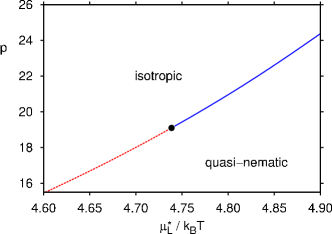
Figure 2: Phase diagram of Eq. (1) in grand canonical representation, with the transition chemical potential $\mu^{\star}_{L}$ on the horizontal axes, and the exponent $p$ on the vertical one (data apply to $L=40$; on the scale of the graph, finite-size effects are small). The line separates isotropic from quasi-nematic phases. The isotropic $\leftrightarrow$ quasi-nematic transition is continuous and of the Kosterlitz-Thouless type when $p<p_{\rm t}$ (dashed) and first-order (solid) when $p>p_{\rm t}$. In the first-order regime, there is a density gap between the phases. The dot, at $p_{\rm t}\approx 19.1$, is the tricritical point obtained via finite-size scaling. At the tricritical point, also the radial distribution function $g(r)$ decays algebraically.

In Fig. 1, we plot $\Delta\mu=\mu^{\star}_{L}-\mu^{S}_{L}$ versus $1/L$, for several values of the sharpness parameter $p$. For the small value, $p=10$, the transition is of the KT type; for the large value, $p=40$, the transition is first-order; the value $p=20$ is close to the tricritical point, as we will show later. In finite systems $\mu^{\star}_{L}>\mu^{S}_{L}$, giving the impression of two separate transitions. However, $\Delta\mu$ decays to zero with increasing $L$. Hence, in the thermodynamic limit, the finite-size estimates $\mu^{\star}_{L}$ and $\mu^{S}_{L}$ are identical, i.e. the statepoint where the density fluctuations are maximal coincides with the maximum of the orientational fluctuations.

For each value of $p$, there is thus only one transition chemical potential, implying that the line of KT transitions joins the line of first-order transitions, as is required for a tricritical point. Fig. 2 shows the phase diagram, i.e. $\mu^{\star}_{L}$ versus $p$, which indeed yields a smooth curve. This curve separates the (low density) isotropic phase, from the (high density) quasi-nematic phase (it does not say anything about the nature of the transition between the phases; this is studied later). In what follows, we will base our analysis on the finite-size estimator $\mu^{\star}_{L}$.

III.2 Structural properties of the bulk phases

We now address the structural properties of the isotropic and quasi-nematic phase. As stated earlier, both phases are characterized by short-ranged positional order. To show this, we consider the static structure factor, $S(\vec{q})=\langle(1/N)|\sum_{i=1}^{N}\exp(\imath\vec{q}\cdot\vec{r}_{i})\,|^{2}\rangle$, with the sum over all particles, $\vec{r}_{i}$ the position of the $i$-th particle, wave vectors $\vec{q}=2\pi(n_{x},n_{y})/L$ with integers $n_{x}$ and $n_{y}$, and $\langle\cdot\rangle$ an ensemble average (in what follows, we use the angular averaged $S(q)$, where $q=|\vec{q}|$). Note that $S(q)$ is the Fourier transform of the radial distribution function $g(r)$, so both these quantities contain the same information.

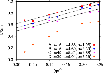
Figure 3: Static structure factor $1/S(q)$ versus $q^{2}$ in the limit $q\to 0$ for various statepoints $A-D$ as indicated (data apply to $L=40$). The statepoints $A-C$ are pure phases, taken well away from the transition line, corresponding to the isotropic phase $(A)$ and the quasi-nematic phase $(B,C)$. The dashed lines for $A-C$ are linear fits and confirm the Ornstein-Zernike form. The statepoint $D$ is taken on the phase transition line, using $p=p_{\chi}(L)$ of the compressibility maximum. In this case, strong deviations from the Ornstein-Zernike formula are observed.

For chemical potentials $\mu$ away from the transition value $\mu^{\star}_{L}$, the $q\to 0$ limit of $S(q)$ is well described by the Ornstein-Zernike form, $1/S(q)=A(1+\xi^{2}_{r}q^{2})$, with $\xi_{r}$ the positional correlation length, and $A\equiv 1/S(0)=\langle N\rangle/(\langle N^{2}\rangle-\langle N\rangle^{2})$ Hansen and McDonald (1986). Some examples are shown in Fig. 3 (statepoints $A-C$). The lines are linear fits, which for the correlation length yield typical values $\xi_{r}/a\sim 1.6-1.7$, i.e. short-ranged. Furthermore, the intercept of the fits is finite, $A>0$, which means that the density fluctuations are not diverging. Hence, as far as the positional order is concerned, the isotropic and quasi-nematic phase are both disordered fluids.

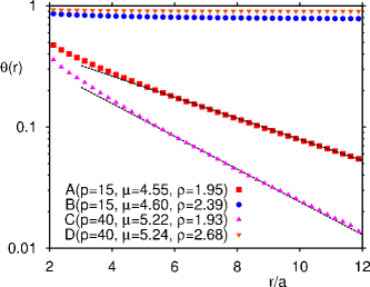
Figure 4: The orientational correlation function $\theta(r)$ for various statepoints $A-D$ as indicated (data apply to $L=40$; note the logarithmic vertical scale). All statepoints correspond to pure phases: isotropic $(A,C)$, and quasi-nematic $(B,D)$. In the isotropic phase, $\theta(r)$ decays exponentially; dashed lines show the corresponding fit. In the quasi-nematic phase, much slower (algebraic) decay is observed.

Next, we consider the orientational correlation function, $\theta(r)=\langle 2(\vec{d}_{i}\cdot\vec{d}_{j})^{2}-1\rangle^{\prime}$ Frenkel and Eppenga (1985), where $\langle\cdot\rangle^{\prime}$ is an ensemble average over all pairs of particles $i-j$ for which $r_{ij}=r$ (in simulations, $\theta(r)$ is collected as a histogram). Some typical examples are shown in Fig. 4, where all the statepoints were chosen away from the phase transition. In the isotropic phase $(A,C)$, the orientational correlations decays exponentially, $\theta(r)\propto\exp(-r/\xi_{\theta})$, with $\xi_{\theta}/a\sim 3-5$ obtained by fitting. In the quasi-nematic phase $(B,D)$, the decay is much slower, and best fitted with a power law, $\theta(r)\propto 1/r^{\eta_{\theta}}$, with $\eta_{\theta}$ being a small positive exponent. Hence, in the quasi-nematic phase, the orientational correlation length $\xi_{\theta}$ is infinite.

To summarize: The isotropic phase of Eq. (1) is characterized by exponential decay of the positional and orientational correlations (both $\xi_{r}$ and $\xi_{\theta}$ being finite). In the quasi-nematic phase, the positional correlations still decay exponentially (finite $\xi_{r}$), while the orientational correlations decay algebraically $(\xi_{\theta}\to\infty)$.

III.3 Nature of the phase transition

Figure 5: (a) Example distribution $W\equiv\ln P(\rho)$ for $p=75$ and $L=15$. The extrema $X(\rho_{X},W_{X})$, $X\in\{A,B,C\}$, define the order parameter $\Delta=\rho_{C}-\rho_{A}$, the coexistence diameter $\delta=(\rho_{C}+\rho_{A})/2$, and the barrier $\Delta F=(W_{A}+W_{C})/2-W_{B}$. (b) Susceptibility $\chi$ versus $p$ for $L=25,30,35,40$ (bottom to top). The curves reach finite maximum values $\chi_{\rm max}(L)$ at $p=p_{\chi}(L)$. (c) Susceptibility maximum $\chi_{\rm max}(L)$ versus $L$. (d) Order parameter $\Delta$ at $p=p_{\chi}(L)$ versus $L$. The dashed curves in (c,d) are power law fits.

We now consider the nature of the isotropic $\leftrightarrow$ quasi-nematic transition, and how the transition type changes with the sharpness parameter $p$. To this end, we follow the path $p(\mu^{\star}_{L})$ in the phase diagram of Fig. 2, and record how the distribution $P(N)$, and the quantities derived from it, vary along it (i.e. for each value of $p$, the chemical potential is tuned such that the variance in the particle number is maximized). For large $p$, where the transition is strongly first-order Wensink and Vink (2007), $P(N)$ is bimodal. An example is shown in Fig. 5(a). The presence of two peaks implies two-phase coexistence (to this end, it may be useful to interpret minus $\ln P(N)$ as the free energy of the system). The left (right) peak corresponds to the isotropic (quasi-nematic) phase. The distance between the peaks reflects the density gap between the phases, which we take as the order parameter $\Delta$ of the transition. It is numerically convenient to compute the order parameter as $\Delta=\langle|M|\rangle/L^{2}$, $M=N-\langle N\rangle$. Similarly, we introduce the order parameter fluctuations (susceptibility) $\chi=\left(\langle M^{2}\rangle-\langle|M|\rangle^{2}\right)/L^{2}$ Orkoulas et al. (2000).

At the tricritical point, $p=p_{\rm t}$, the density gap $\Delta$ vanishes. To locate this point, we perform a finite-size scaling analysis. Fig. 5(b) shows $\chi$ versus $p$ for several $L$. We note that each curve reveals a maximum. The value of $p$ at the maximum defines $p_{\chi}(L)$, the corresponding value of the susceptibility defines $\chi_{\rm max}(L)$ (we emphasize that both these quantities are $L$-dependent). The fact that $\chi_{\rm max}(L)$ increases with $L$ indicates that, at the tricritical point $p_{\rm t}=\lim_{L\to\infty}p_{\chi}(L)$, the susceptibility diverges. We observe a power-law increase, $\chi_{\rm max}(L)\propto L^{\omega_{1}}$, with $\omega_{1}\approx 1.0\pm 0.03$ obtained by fitting [Fig. 5(c)]. For the order parameter, measured at $p=p_{\chi}(L)$, we observe a power-law decay, $\Delta\propto L^{-\omega_{2}}$, where a fit yields $\omega_{2}\approx 0.5\pm 0.03$ [Fig. 5(d)]. Note that the exponents obey hyperscaling, $\omega_{1}+2\omega_{2}=d=2$, as is characteristic of critical and tricritical transitions Wilding and Nielaba (1996). This implies that, at the tricritical point, the distribution $P(N)$ is scale invariant.

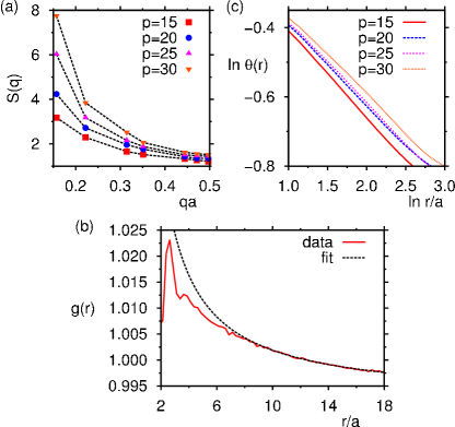
Figure 6: Structural properties measured along the path $p(\mu^{\star}_{L})$, i.e. the line of isotropic $\leftrightarrow$ quasi-nematic phase transitions of Fig. 2, restricted to the range $p\leq p_{\chi}(L)$. The data apply to $L=40$, for which $p_{\chi}(L)\sim 30$. (a) The static structure factor $S(q)$ for various values of $p$ as indicated. As $p\to p_{\chi}(L)$, $S(q\to 0)$ strongly increases, consistent with a critical point at $p_{\chi}(L)$. (b) The radial distribution function $g(r)$ at $p_{\chi}(L)$, together with a fit to Eq. (7), the fit range being $10<r/a<18$. (c) The orientational correlation function $\theta(r)$ for several values of $p$. Note the double-logarithmic scale! The decay of $\theta(r)$ is algebraic.

The diverging susceptibility is also manifested by the static structure factor measured along the path $p(\mu^{\star}_{L})$. As $p\to p_{\chi}(L)$, $S(q\to 0)$ strongly increases, consistent with diverging order parameter fluctuations [Fig. 6(a)]. Note that in Fig. 6 the tricritical point is approached from below, i.e. starting with small $p$. This was done for convenience: Approaching the tricritical point from above would require $S(q)$ to be measured for the isotropic and quasi-nematic phase separately, since these phases coexist when $p>p_{\chi}(L)$. At the tricritical point, $S(q)$ strongly deviates from the Ornstein-Zernike formula, with $1/S(q\to 0)$ now tending to zero [Fig. 3, statepoint $D$]. A diverging susceptibility implies that, at the tricritical point, also the positional correlations decay algebraically, i.e. $\xi_{r}\to\infty$. In 2D, the radial distribution function should then decay asymptotically as Pelissetto and Vicari (2002)

$$\lim_{r\to\infty}g(r)=c_{1}+c_{2}/r^{\eta_{r}}\quad,$$ (7)

with $\eta_{r}=2-\omega_{1}\sim 1.0$, and constants $c_{i}$. Fig. 6(b) shows that $g(r)$ at $p_{\chi}(L)$ is indeed well described by this form, where $\eta_{r}=1$ was imposed, and the constants $c_{i}$ were fitted.

In Fig. 6(c), we plot the orientational correlation function $\theta(r)$ measured along the path $p(\mu^{\star}_{L})$. All along the path $p(\mu^{\star}_{L})$, $\theta(r)$ decays algebraically. At $p_{\chi}(L)$, the exponent of the algebraic decay of the orientational correlations $\eta_{\theta}\sim 0.22$, i.e. much slower than the decay of the positional correlations. In contrast, the radial distribution function $g(r)$ decays algebraically only at the tricritical point. The simultaneous divergence of two order parameter fluctuations (here: density and orientation), implied by the algebraic decay of the corresponding correlation functions, is characteristic of tricritical phenomena.

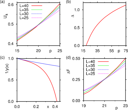
Figure 7: (a) Binder cumulant $U_{4}$ versus $p$ for several $L$. The intersections mark $p_{\rm t}$. (b) Order parameter $\Delta$ versus $p$ obtained following Kim and Fisher Kim and Fisher (2005). At $p_{\rm t}$, the order parameter vanishes. (c) The (inverse) scaling function $y(x)$ of the Kim-Fisher algorithm (solid). Also shown is the $x\to 0$ limiting form (dashed), which our data indeed approach. (d) The barrier $\Delta F$ versus $p$ for several $L$. At the tricritical point, the curves for different $L$ intersect.

III.4 Determination of $p_{\rm t}$

Finally, we determine $p_{\rm t}$. The standard approach is to consider the Binder cumulant $U_{4}=\langle M^{2}\rangle^{2}/\langle M^{4}\rangle$; owing to hyperscaling, the latter is $L$-independent at $p_{\rm t}$ Binder (1981). In Fig. 7(a), we plot $U_{4}$ versus $p$ for various $L$. We observe a scatter of intersections, between $18.9<p<20.4$, providing a rough estimate of $p_{\rm t}$ (corrections to scaling appear to be quite strong, and so we restrict the analysis to the largest four system sizes in what follows). A more precise estimate of $p_{\rm t}$ is obtained using the complete scaling algorithm of Kim and Fisher Kim and Fisher (2005). For the practical implementation of the latter, our $p$-extrapolation scheme, i.e. Eq. (4), is absolutely crucial, since data over a wide range in $p$ are required (stretching from the first-order to the tricritical regime). The principal output of the complete scaling algorithm is the $L\to\infty$ value of the order parameter $\Delta$ as a function of $p$ [Fig. 7(b)]. From this, we conclude $p_{\rm t}=19.1\pm 0.1$, i.e. the value where $\Delta$ vanishes. Note that this estimate is consistent with the cumulant intersections.

A second output of the complete scaling algorithm is a scaling function $y(x)$, defined in the Appendix, which is characteristic of the universality class [Fig. 7(c)]. In the limit $x\to 0$, $y(x)=1+x/2$, while at some $x_{\rm c}>0$, $y(x)$ diverges. We obtain $x_{\rm c}\approx 0.42$. As a last method to obtain $p_{\rm t}$, we consider the barrier $\Delta F$ of $\ln P(N)$, defined in Fig. 5(a) as the average height of the peaks (A and B) minus the height at the minimum (C). The barrier increases (decreases) with $L$ for $p>p_{\rm t}$ ($p<p_{\rm t}$), and remains $L$-independent at $p_{\rm t}$ Binder (1982); Lee and Kosterlitz (1990). The variation of $\Delta F$ with $p$ for several $L$ is shown in Fig. 7(d). At the tricritical point, the curves for different $L$ intersect, at values of $p$ consistent with those of the cumulant analysis.

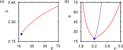
Figure 8: (a) Coexistence diameter $\delta$ versus $p$ obtained following Ref. Kim, 2005. (b) $L\to\infty$ phase diagram of Eq. (1), showing the binodal (solid) and diameter (dashed). The tricritical point (dots) is at $p_{\rm t}=19.1$ and $\rho_{\rm c}=2.205$.

III.5 Phase diagram in $(\rho,p)$-representation

For completeness, we still compute the $L\to\infty$ phase diagram in $(p,\rho)$-representation. Kim also provides a scaling algorithm to obtain the $L\to\infty$ coexistence diameter $\delta$ from finite-size simulation data Kim (2005). The latter is defined as the average density of the isotropic and quasi-nematic phase [Fig. 5(a)]. In Fig. 8(a), we plot $\delta$ versus $p$. The order parameter and coexistence diameter yield the binodal, i.e. the density of the isotropic ($\delta-\Delta/2$) and quasi-nematic phase ($\delta+\Delta/2$) as a function of $p$ [Fig. 8(b)]. The region inside the binodal marks the statepoints where both these phases coexist. Note that the isotropic and quasi-nematic branches form a “kink” at the tricritical point, in agreement with a mean-field treatment of Eq. (1) Wensink and Vink (2007). Not shown in the phase diagrams of Fig. 8 is the line of continuous KT transitions that commence below the tricritical point.

IV Discussion and summary

In summary, we have considered the crossover of the Kosterliz-Thouless transition in 2D liquid crystals from continuous to first-order. Our main result is that, at the crossover, a tricritical point occurs. At the tricritical point, both the positional and orientational correlations decay algebraically. The algebraic decay of positional order enhances the spectrum of possible structure in 2D liquid crystals, since positional order in quasi-nematic phases is typically assumed to decay exponentially.

It may be that the tricritical point we found is universal, in the sense that any model with sufficiently sharp interactions and 2D positional/vector degrees of freedom would yield the same set of tricritical exponents, $\omega_{1}$ and $\omega_{2}$. To test this hypothesis, it would be interesting to apply the analysis of this work to lattice-based models, such as the one studied by Domany and co-workers Domany et al. (1984). In that case, the analysis could be based on the energy distribution $P(E)$, which also becomes bimodal when the transition is first-order. Such an analysis is furthermore interesting because there is not yet consensus about how the first-order transition ends. The simultaneous divergence of the density and orientational fluctuations observed by us indicates a tricritical point, while studies of lattice-based models also report critical point behavior Jonsson et al. (1993). According to Ref. van Enter and Shlosman, 2007, in 2D spatial dimensions, lowering $p$ leads to a 2D Ising critical point, but this assumes the absence of a KT transition fn (2). In agreement with this, using 2D spatial dimensions and 3D vector spins (Heisenberg case), a KT transition is not expected (orientational correlations always decay exponentially). In that case, numerical simulations Blöte et al. (2002) are consistent with a 2D Ising critical point, i.e. $\omega_{1}=7/4$ and $\omega_{2}=1/8$.

The present analysis was largely facilitated by a method to extrapolate simulation data in the sharpness parameter $p$. However, it is by no means restricted to the model of Eq. (1), and can be applied to any variable in any potential, provided an explicit expression for the expansion Eq. (4) can be given. In particular, it can also be used to extrapolate in field variables, i.e. the type of variables (temperature, chemical potential) for which histogram reweighting Ferrenberg and Swendsen (1988) was originally intended. Due to its modest storage requirements, our scheme could prove attractive even then. For an explicit demonstration, we refer the reader to the Appendix of Ref. Vink, 2014, where extrapolations in temperature are performed in this manner. For the future, it would be useful to develop a more rigorous version of Eq. (5) to combine data obtained for different values of the control parameters, along the lines of the multiple-histogram method Ferrenberg and Swendsen (1989).

Appendix A Kim-Fisher scaling algorithm

We still describe the Kim-Fisher scaling algorithm Kim and Fisher (2005) that was used to generate the data of Fig. 7(b,c). For a fixed sharpness parameter $p$ and system size $L$, it is straightforward to measure $U_{4}$ and $\rho=\langle N\rangle/L^{2}$ as a function of $\mu$. A plot of $U_{4}$ versus $\rho$, which is thus parameterized by $\mu$, reveals two minima. The location of the minimum at low density is denoted $\rho^{-}(L,p)$, with $Q^{-}(L,p)$ the corresponding cumulant value. Similarly, the location of the minimum at high density is denoted $\rho^{+}(L,p)$, with $Q^{+}(L,p)$ the corresponding cumulant value. The purpose of the scaling algorithm is to evaluate the order parameter $\Delta$ as a function of $p$ in the thermodynamic limit: $\Delta(p)=\lim_{L\to\infty}(\rho^{+}(L,p)-\rho^{-}(L,p))/2$. To this end, one defines the quantities

$$Q_{\rm min}(L,p) \equiv \frac{Q^{+}(L,p)+Q^{-}(L,p)}{2}\quad,$$ (8)

$$x(L,p) \equiv Q_{\rm min}(L,p)\ln\left[\frac{4}{eQ_{\rm min}(L,p)}\right]\quad,$$ (9)

$$y(L,p) \equiv \frac{\rho^{+}(L,p)-\rho^{-}(L,p)}{\Delta(p)}\quad.$$ (10)

The algorithm starts in the first-order regime, i.e. with a large value of $p$. The peaks in $P(N)$ are then well separated and the free energy barrier $\Delta F$ will be large, as in Fig. 5(a). In this regime, it can be shown rigorously that the points $(x,y)$ of different system sizes $L$, should all collapse onto the line $y=1+x/2$. Recall that $\Delta(p)$ in Eq. (10) is the order parameter in the thermodynamic limit at the considered $p$, precisely the quantity of interest, which may thus be obtained by fitting until the best collapse onto $y=1+x/2$ occurs. Next, $p$ is chosen closer to the critical point, the points $(x,y)$ are calculated as before, but this time around $\Delta(p)$ is chosen such that the new data set joins smoothly with the previous one, yielding an estimate of the order parameter at the new $p$. This procedure is repeated as closely as possible to the tricritical point, where $\Delta$ vanishes, yielding an estimate of $p_{\rm t}$.