Abstract

We review, in the first part of this work, many pioneering works on supersymmetry and organize these results to show how supersymmetric quantum field theories arise from spin-statistics, Nœther and a series of no-go theorems. We then introduce the so-called superspace formalism dedicated to the natural construction of supersymmetric Lagrangians and detail the most popular mechanisms leading to soft supersymmetry breaking.

As an application, we describe the building of the Minimal Supersymmetric Standard Model and investigate current experimental limits on the parameter space of its most constrained versions. To this aim, we use various flavor, electroweak precision, cosmology and collider data. We then perform several phenomenological excursions beyond this minimal setup and probe effects due to non-minimal flavor violation in the squark sector, revisiting various constraints arising from indirect searches for superpartners.

Next, we use several interfaced high-energy physics tools, including the FeynRules package and its UFO interface that we describe in detail, to study the phenomenology of two non-minimal supersymmetric models at the Large Hadron Collider. We estimate the sensitivity of this machine to monotop production in $R$-parity violating supersymmetry and sgluon-induced multitop production in $R$-symmetric supersymmetry. We then generalize the results to new physics scenarios designed from a bottom-up strategy and finally depict, from a theorist point of view, a search for monotops at the Tevatron motivated by these findings.

Contents

1. 1 Introduction
2. 2 Supersymmetric quantum field theories
   1. 2.1 The Poincaré superalgebra
      1. 2.1.1 Quantum field theories and symmetries
      2. 2.1.2 The Coleman-Mandula theorem
      3. 2.1.3 Lie superalgebra
      4. 2.1.4 The $N=1$ Poincaré superalgebra
   2. 2.2 Representations of the $N=1$ Poincaré superalgebra
      1. 2.2.1 Representations of the Poincaré algebra
      2. 2.2.2 Representations of the Poincaré superalgebra: general features
      3. 2.2.3 Massless representations of the Poincaré superalgebra
      4. 2.2.4 Massive representations of the Poincaré superalgebra
   3. 2.3 The superspace formalism
      1. 2.3.1 Supercharges and superderivatives in the superspace
      2. 2.3.2 General superfields
      3. 2.3.3 Chiral superfields
      4. 2.3.4 Vector superfields
   4. 2.4 From superfields to Lagrangians
      1. 2.4.1 Chiral Lagrangians
      2. 2.4.2 Vector Lagrangians
      3. 2.4.3 Gauge interactions of chiral superfields
      4. 2.4.4 Non-renormalizable and renormalizable supersymmetric gauge theories
3. 3 Supersymmetry in FeynRules
   1. 3.1 The FeynRules package
      1. 3.1.1 Basic features of the FeynRules package
      2. 3.1.2 Preamble of the model file: information and indices
      3. 3.1.3 Defining gauge groups
      4. 3.1.4 Declaring the model parameters
      5. 3.1.5 Implementing fields and particles
      6. 3.1.6 Implementing Lagrangians
      7. 3.1.7 Running FeynRules
      8. 3.1.8 Interfaces to Monte Carlo event generators
   2. 3.2 The Universal FeynRules output - the UFO
      1. 3.2.1 Basic features
      2. 3.2.2 Initialization and structure of the objects and functions
      3. 3.2.3 Implementing the model particle content
      4. 3.2.4 Implementing the model parameters
      5. 3.2.5 Implementing the interactions of the model
   3. 3.3 Implementing supersymmetric models in FeynRules
      1. 3.3.1 Calculations in superspace
      2. 3.3.2 Supercharges, superderivatives and supersymmetric transformations
      3. 3.3.3 Implementing and manipulating superfields in FeynRules
      4. 3.3.4 Automatic generation of supersymmetric Lagrangians
   4. 3.4 Supersymmetric transformations
      1. 3.4.1 Variation of chiral superfields
      2. 3.4.2 Variation of general superfields
      3. 3.4.3 Vector superfields in the Wess-Zumino gauge
   5. 3.5 Non-renormalizable supersymmetric model building
4. 4 Supersymmetry breaking
   1. 4.1 Supersymmetry breaking: general features
      1. 4.1.1 Motivations for softly broken supersymmetric theories
      2. 4.1.2 The Goldstone theorem for supersymmetry
      3. 4.1.3 Properties of the goldstino field
      4. 4.1.4 The supertrace constraint
   2. 4.2 Examples of soft supersymmetry-breaking mechanisms
      1. 4.2.1 Supergravity: general features
      2. 4.2.2 Gravity-mediated supersymmetry breaking
      3. 4.2.3 Gauge-mediated supersymmetry breaking
      4. 4.2.4 Anomaly-mediated supersymmetry breaking
   3. 4.3 Renormalization group equations for supersymmetry
5. 5 The Minimal Supersymmetric Standard Model
   1. 5.1 Construction of the model
      1. 5.1.1 Field content
      2. 5.1.2 Supersymmetry-conserving Lagrangian
      3. 5.1.3 Supersymmetry-breaking Lagrangian
      4. 5.1.4 Electroweak symmetry breaking and particle mixings
      5. 5.1.5 Supersymmetry-breaking models in the MSSM framework
   2. 5.2 Main phenomenological features of the MSSM
      1. 5.2.1 The hierarchy or the fine-tuning problem
      2. 5.2.2 Gauge coupling unification
      3. 5.2.3 Consequences of $R$-parity conservation
   3. 5.3 Constraints from low-energy and electroweak precision measurements
      1. 5.3.1 Rare $B$-meson decays
      2. 5.3.2 $B$-meson oscillations
      3. 5.3.3 The anomalous magnetic moment of the muon
      4. 5.3.4 The electroweak $\rho$-parameter
      5. 5.3.5 Summary
   4. 5.4 Cosmological aspects
      1. 5.4.1 General features
      2. 5.4.2 Neutralino dark matter in the constrained MSSM
      3. 5.4.3 Gravitino dark matter in gauge-mediated supersymmetry breaking
      4. 5.4.4 Neutralino dark matter with anomaly-supersymmetry breaking
   5. 5.5 Direct constraints
   6. 5.6 Motivation for going beyond the MSSM
6. 6 Searching for non-minimal supersymmetry at hadron colliders
   1. 6.1 Beyond minimal supersymmetry: two examples
      1. 6.1.1 $R$-parity violation
      2. 6.1.2 The minimal $R$-symmetric supersymmetric model
   2. 6.2 Implementation of supersymmetric models in FeynRules
      1. 6.2.1 The MSSM
      2. 6.2.2 The MSSM with $R$-parity violation
      3. 6.2.3 The minimal $R$-symmetric supersymmetric theory
   3. 6.3 From FeynRules to MadGraph 5
   4. 6.4 Monotop production in the MSSM with $R$-parity violation
      1. 6.4.1 Benchmark scenario and process of interest
      2. 6.4.2 Phenomenological investigations at 7 TeV
   5. 6.5 Sgluon-induced multitop production in $R$-symmetric supersymmetry
      1. 6.5.1 Benchmark scenario and process of interest
      2. 6.5.2 Phenomenological investigations at 7 TeV
7. 7 From non-minimal supersymmetry to effective field theories
   1. 7.1 Effective theories inspired by non-minimal supersymmetry
      1. 7.1.1 An effective field theory for monotop production
      2. 7.1.2 A simplified model for sgluon production and decays at the LHC
   2. 7.2 Monte Carlo simulations of the Standard Model background
      1. 7.2.1 Simulation setup
      2. 7.2.2 Single boson production in association with jets
      3. 7.2.3 Single and pair production of top quarks in association with jets
      4. 7.2.4 Diboson production in association with jets
      5. 7.2.5 Rare Standard Model processes
   3. 7.3 Monotop production with a CMS-like detector
      1. 7.3.1 Object definitions
      2. 7.3.2 Seeking monotops at the LHC
   4. 7.4 Sgluon-induced multitop production with an ATLAS-like detector
      1. 7.4.1 Object definitions
      2. 7.4.2 Searching for sgluons via multitop events at the LHC
8. 8 When theory meets experiment
   1. 8.1 Search for monotops with the CDF detector
      1. 8.1.1 Analysis strategy for monotop searches with the CDF detector
      2. 8.1.2 Results of the first monotop search at a hadron collider
   2. 8.2 Conclusions of a search for sgluons with the ATLAS detector
9. 9 Conclusions
10. A Conventions
    1. A.1 Lorentz indices
    2. A.2 Spinor indices
    3. A.3 Pauli and Dirac matrices
    4. A.4 Grassmann variables

Chapter 1 Introduction

After almost fifty years, the Standard Model of particle physics [1, 2, 3, 4, 5, 6, 7, 8, 9, 10] has been proved to be a successful theory to describe all experimental high-energy physics data. It however leaves, despite its success, many important questions open without providing any satisfactory answer. Among those, one finds the unexplained large hierarchy between the electroweak and the Planck scales, the absence of a mechanism leading to neutrino oscillations, the unknown origins of dark matter and of the cosmological constant as well as the strong $CP$-problem. Consequently, the Standard Model is widely acknowledged as the low-energy limit of a more fundamental theory. The recent discovery of a Higgs boson [11, 12] that seems to feature properties as expected from the Standard Model reinforces this picture. This first observation of a particle intrinsically unstable with respect to quantum corrections indeed implies either a non-natural extreme fine-tuning or a stabilization arising from a new physics sector which will emerge at scales that we will probe soon.

As a result, model building activities in a beyond the Standard Model framework have been very intense during the last decades. Among the leading candidates for new physics, one finds extensions of the Standard Model where its $SU(3)_{c}\times SU(2)_{L}\times U(1)_{Y}$ gauge group is embedded into a larger structure, such as, e.g., $SU(5)$, $SO(10)$ or $E_{6}$ [13, 14, 15, 16, 17]. In those contexts, the Standard Model quark and lepton fields are encompassed into one or several representations of the extended gauge group, together with possible additional matter content, and the three gauge coupling constants have their strength unified at high energies due to new effects in their renormalization group running. Those models have also interesting additional properties, such that some of them could easily include an explanation for neutrino masses or provide a mechanism leading to the quantization of the electric charge. However, Grand Unified Theories have often difficulties to get in agreement with the measured value for the electroweak mixing angle or even to forbid the proton to decay in the case of the simplest extended gauge groups.

Another popular way to extend the Standard Model and solve at the same time the hierarchy problem is to modify the structure of spacetime and include additional dimensions [18, 19, 20, 21]. In this case, the Minkowski spacetime is extended by either a compact manifold, as in pioneering extra-dimensional models, or by an orbifold, as in more modern approaches. The large value of the Planck scale is then a consequence of the presence of the extra dimensions. Moreover, each field living in the extra-dimensions can be seen as an usual four-dimensional field coming together with a series of more massive excitations that can be possibly detected at collider experiments.

In this work, we choose to focus on another type of symmetry, dubbed supersymmetry, which naturally extends the Poincaré algebra and links the fermionic and bosonic degrees of freedom of the theory [22, 23, 24, 25, 26, 27, 28, 29, 30]. In particular, the minimal phenomenologically viable supersymmetric model resulting from the direct supersymmetrization of the Standard Model, the so-called Minimal Supersymmetric Standard Model (MSSM) [31, 32], is one of the most studied options for new physics, both at the theoretical and experimental levels. In addition of associating with each fermion of the theory one bosonic superpartner, and vice versa, weak scale supersymmetry also allows to solve several of the conceptual problems of the Standard Model. Accounting for the supersymmetric degrees of freedom leads to a natural unification of the three gauge couplings when run to higher energies [33, 34, 35, 36, 37, 38] and stabilizes all scalar masses with respect to quantum corrections, solving hence the hierarchy problem [39]. Furthermore, many supersymmetric models include a particle candidate for explaining the presence of dark matter in the Universe [40, 41]. However, the superpartners of the Standard Model particles have not been observed, so that supersymmetry must be broken at low-energy. In order not to reintroduce quadratically divergent quantum corrections in the theory, this breaking must be soft and is therefore expected to shift the supersymmetric particle masses around the TeV scale.

Consequently, the quest for supersymmetric particles is one of the main topics of the experimental program at the Large Hadron Collider (LHC) at CERN. However, there is no sign for a single superpartner so far and the latest results of the general purpose experiments ATLAS and CMS are currently pushing the bounds on the masses of the superpartners to higher and higher scales [42, 43]. In other words, the supersymmetric parameter space turns out to be more and more constrained. However, most analyses are only valid in the context of the so-called constrained MSSM (cMSSM) framework, where the 105 free parameters of the minimal supersymmetric model are reduced to a set of four parameters and a sign, or for very specific simplified models inspired by the cMSSM. In contrast, there are much broader classes of supersymmetric theories valuable to be studied both from a theoretical point of view and from an experimental one. The results obtained from such studies could be further employed to design new search strategies for new physics models, even possibly not supersymmetric when one accounts for a possible recasting of the experimental analyses.

Phenomenological studies of such non-minimal supersymmetric models in the context of hadron-collider experiments are often based on the use of Monte Carlo event generators. In this framework, a proper modeling of the strong interactions, including parton showering, fragmentation and hadronization, is essential for achieving a realistic description of the hadronic collisions. The latter is efficiently provided by packages such as Pythia [44, 45, 46], Sherpa [47, 48] or Herwig [49, 50, 51, 52]. However, any new physics signal is expected to occur at the level of the underlying hard interaction. As a consequence, lots of effort have been put into the development of matrix-element generators such as AlpGen [53], CompHep and CalcHep [54, 55, 56, 57], Helac [58, 59], MadGraph and MadEvent [60, 61, 62, 63, 64], Sherpa [47, 48] and Whizard [65, 66], that allow for the generation of parton-level events of large classes of beyond the Standard Model theories.

Historically, these packages have only supported the Standard Model and a restricted subset of new physics theories, the reasons lying in the complexity of the implementation of validated and ready-to-be-used model files. This task indeed requires, first, a precise knowledge of the Monte Carlo program itself, second, the implementation of thousands of lines of code associated with the Feynman rules of the model and third, a long and tedious process of debugging. Implementing new models into these simulation packages has however recently drastically improved. Parton-level matrix element generators have firstly begun to establish more general model formats so that a less intimate knowledge of their internal code is now necessary [67]. Secondly, several external programs, such as LanHep [68, 69, 70, 71, 72], FeynRules [73, 74, 75, 76, 77, 78, 79, 80] and Sarah [81, 82, 83, 84], have been developed in order to allow the user to define a model via its Lagrangian rather than via the set of its individual Feynman rules.

Thanks to the above-mentioned packages, a systematic investigation of the phenomenology of any new physics model has been rendered possible and straightforward following the path of a top-down approach. In this context, the theory is first defined by its particle content, gauge symmetries, free parameters and Lagrangian. Next, relevant benchmark scenarios that are both theoretically motivated and not experimentally excluded are constructed and finally employed for predicting the model signatures at high-energy experiments. The design of such benchmarks is however not an easy task, as many model parameters enter and cannot be fixed by the present constraints. The conception of benchmarks is thus in general driven by simplicity, which introduces at the same time some bias in the definition of signatures called typical for a given model. Furthermore, a given signature is neither related to a single benchmark nor to a specific model itself. Universal extra dimensions and supersymmetry share, for instance, very similar signatures starting from the pair production of new states followed by their cascade decays into an invisible state, jets and charged leptons.

For these reasons, it is useful to perform, in parallel to top-down phenomenological investigations, alternative studies starting from a final state signature. In order to model the mechanisms leading to the production of a specific signature, a Lagrangian with a minimal set of effective operators is usually supplemented to the Standard Model one. Results obtained in this framework can then be reinterpreted, in a second step, in the context of several beyond the Standard Model theories simultaneously.

In this work, we have adopted a more pragmatic choice and rely both on the top-down and bottom-up approaches for probing new physics at colliders. We have first followed a top-down path and started by studying well defined non-minimal supersymmetric theories. We have analyzed specific signatures predicted by the models under consideration and have designed several search strategies allowing for a possible observation of the associated signals at the LHC. To this aim, we have performed simulations of proton-proton collisions that have occurred at both past LHC runs, at respective center-of-mass energies of 7 TeV and 8 TeV, and analyzed the generated events within the MadAnalysis 5 framework [85]. More into details, events have been simulated by means of the automated Monte Carlo program MadGraph 5, whose necessary UFO model libraries have been produced directly from the respective Lagrangians by making use of the FeynRules package. Accurate descriptions of both the new physics signals and the different contributions to the Standard Model background have been obtained by relying, on the one hand, on multiparton matrix-element merging of leading-order event samples with different final state multiplicities [86, 87], and, on the other hand, on results for total rates computed at the next-to-leading order and next-to-next-to-leading order accuracies in QCD. Moreover, advanced simulations of the ATLAS and CMS detector responses have been performed with the Delphes program [88].

In a second stage, we employ the investigated signatures as a starting point and study them in a more general bottom-up context, well beyond the initial non-minimal supersymmetric frameworks. We construct effective Lagrangians with a set of new interactions leading to the production of the final states under consideration, possibly including mediation by additional new states. Using the search strategies developed in the supersymmetric cases as guidelines, we make use of Monte Carlo simulations as above to extract the parameter space regions of the bottom-up inspired theoretical models that can be reached by the LHC.

Finally, as the last step of this work, we describe (public) experimental searches that have been motivated by our phenomenological investigations. This allows this manuscript to illustrate a full chain linking theory to experiment via both bottom-up and top-down phenomenological excursions beyond the Standard Model.

In the next chapter (Chapter 2), we describe in full generality the building of a supersymmetric theory from very basic principles, namely the spin-statistics theorem [89], the Nœther theorem [90], as well as a series of no-go theorems [91, 92]. We show how the only knowledge of these theorems leads unavoidably to the Poincaré superalgebra underlying phenomenologically relevant supersymmetric models. We then move to a detailed description of the superspace formalism [27, 28, 29], the natural approach for the building of supersymmetric Lagrangians. The content of this chapter is based on the supersymmetry lectures given by the author at the University of Louvain-la-Neuve (Belgium) in January-March 2011 as well as on the book (in French) of Ref. [93],

B. Fuks and M. Rausch de Traubenberg,
Supersymétrie : exercices avec solutions,
Ellipses Editions, 2011 (ISBN 978-2-729-86318-0).

Chapter 3 is dedicated to the implementation of supersymmetric models in FeynRules, such a tool allowing for the study of the associated phenomenology by means of Monte Carlo simulations thanks to dedicated interfaces to several automated event generators. We first describe the FeynRules package itself, together with the Universal FeynRules format (UFO) allowing to pass the information from FeynRules to any other program in a very generic way. Emphasis is put on all the tasks that can be automated, reducing in this way the risk of error by the user. Examples of calculations that can be performed using the superspace module of FeynRules are finally provided. The material of this chapter is based on the manual of the version 2.0 of FeynRules [80], on a series of specific papers that have recently appeared [74, 75, 76, 79], as well as on the definition of the UFO conventions [67],

A. Alloul, N. D. Christensen, C. Degrande, C. Duhr and B. Fuks,
FeynRules 2.0, a complete toolbox for tree-level phenomenology,
arXiv:1310.1921 [hep-ph] (submitted to Comput. Phys. Commun.).
N. D. Christensen, P. de Aquino, N. Deutschmann, C. Duhr, B. Fuks, C. Garcia-Cely, O. Mattelaer, K. Mawatari, B. Oexl and Y. Takaesu,
Simulating spin-3/2 particles at hadron colliders,
Eur. Phys. J. C 73 (2013) 2580.
C. Degrande, C. Duhr, B. Fuks, D. Grellscheid, O. Mattelaer and T. Reiter,
UFO - The Universal FeynRules Output,
Comput. Phys. Commun.  183 (2012) 1201-1214.
N. D. Christensen, C. Duhr, B. Fuks, J. Reuter and C. Speckner,
Introducing an interface between Whizard and FeynRules,
Eur. Phys. J. C 72 (2012) 1990.
C. Duhr and B. Fuks,
A superspace module for the FeynRules package,
Comput. Phys. Commun.  182 (2011) 2404-2426.
N. D. Christensen, P. de Aquino, C. Degrande, C. Duhr, B. Fuks, M. Herquet, F. Maltoni and S. Schumann,
A comprehensive approach to new physics simulations,
Eur. Phys. J. C 71 (2011) 1541.

Realistic supersymmetric models must encompass supersymmetry breaking. In Chapter 4, we describe some general features associated with any supersymmetry-breaking model [39, 94, 95, 96, 97, 98, 99] and then turns to a short review of the most popular mechanisms employed to achieve soft supersymmetry-breaking, namely gravity-mediated supersymmetry breaking [100, 101, 102, 103, 104, 105, 106, 107, 108, 109, 110, 111, 112, 113, 114], gauge-mediated supersymmetry breaking [115, 116, 117, 118, 119, 120, 121, 122, 123, 124, 125] and anomaly-mediated supersymmetry breaking [126, 127, 128, 129, 130, 131, 132, 133]. This chapter is based on the above-mentioned book [93], on the lectures given at the University of Louvain-la-Neuve, and on the forthcoming publication [134],

B. Fuks and M. Rausch de Traubenberg,
A supergravity primer,
In preparation.

The theoretical framework developed in Chapter 2 and Chapter 4 is applied, in Chapter 5, to the building of the simplest supersymmetric model, the Minimal Supersymmetric Standard Model [31, 32]. We provide first detailed information on the construction of the model itself. In a second step, we present the most general features of the MSSM, addressing the hierarchy problem, gauge coupling unification, the dark matter problematics and introducing the most common properties of the MSSM concerning the production of supersymmetric particles at colliders. We then establish, in the framework of three minimal MSSM scenarios with a small number of free parameters, the parameter space regions compatible with up-to-date data from low-energy, electroweak precision and flavor physics. A first step towards non-minimal supersymmetric models is next achieved by studying the effects of non-minimal flavor violation in the squark sector. Finally, cosmological aspects are addressed, as well as constraints originating from direct searches for supersymmetric particles at colliders and in particular at the LHC. The results of this chapter are based, on the one hand, on the above-mentioned Ref. [76], Ref. [93], and on the lectures given at the University of Louvain-la-Neuve, as well as on the papers [135, 136, 137],

B. Fuks, B. Herrmann and M. Klasen,
Phenomenology of anomaly-mediated supersymmetry breaking scenarios with non-minimal flavor violation,
Phys. Rev. D 86 (2012) 015002.
B. Fuks, B. Herrmann and M. Klasen,
Flavor violation in gauge-mediated supersymmetry breaking models: experimental constraints and phenomenology at the LHC,
Nucl. Phys.  B 810 (2009) 266-299.
G. Bozzi, B. Fuks, B. Herrmann and M. Klasen,
Squarks and gaugino hadroproduction and decays in non-minimal flavor violating supersymmetry,
Nucl. Phys.  B 787 (2007) 1-54.

In the next chapter (Chapter 6), we describe two non-minimal supersymmetric theories, the MSSM with $R$-parity violation [138] and the minimal version of a supersymmetric theory with an unbroken $R$-symmetry [139, 140, 141]. After implementing both theories into FeynRules, dedicated phenomenological analyses are performed for each of the models by means of Monte Carlo simulations, employing the chain FeynRules-UFO-MadGraph 5-Pythia-Delphes-MadAnalysis 5 for generating and analyzing events including detector response effects. This allows us to investigate one collider signature for each of the two models above, monotop production in $R$-parity violating supersymmetry and multitop production induced by the decay of a pair of sgluon fields as predicted in $R$-symmetric supersymmetric models. We show that one can expect visible signals at the LHC, running at a center-of-mass energy of 7 TeV, in the case of specific benchmark scenarios. The material included in this chapter is based on the work of Ref. [77] for which it also provides extra details,

B. Fuks,
Beyond the Minimal Supersymmetric Standard Model: from theory to phenomenology,
Int. J. Mod. Phys. A 27 (2012) 1230007.

Generalizing the supersymmetric picture, we construct in Chapter 7 two frameworks based on an effective field theory aiming to describe the production of the two new physics signals under consideration. We explore in this way several beyond the Standard Model theories at the same time, although the reinterpretation process in the context of a specific model goes beyond the scope of this work. We hence address, using the chain of tools above, the production of a monotop state and the one of a multitop signature arising from the decay of a pair of sgluons in an effective field theory context. Detailed phenomenological investigations are performed in order to estimate the regions of the parameter spaces of both models covered by the LHC, with 20 fb^-1 of collisions at a center-of-mass energy of 8 TeV. We also provide, in this chapter, extensive details about the simulation of the Standard model background. We review the works of the two published papers of Ref. [142] and Ref. [143] and present new results that have been recently submitted [144],

J. L. Agram, J. Andrea, M. Buttignol, E. Conte and B. Fuks,
Monotop phenomenology at the Large Hadron Collider,
arXiv:1311.6478 [hep-ph] (accepted by Phys. Rev. D).
S. Calvet, P. Gris, B. Fuks and L. Valéry,
Searching for sgluons in multitop events at a center-of-mass energy of 8 TeV,
JHEP 1304 (2012) 043.
J. Andrea, B. Fuks and F. Maltoni,
Monotops at the LHC,
Phys. Rev. D 84 (2011) 074025.

Motivated by our phenomenological results, several experimental searches at hadron colliders have either been achieved or are currently on-going [145, 146, 147, 148]. We dedicate the last chapter of this document, Chapter 8, to the presentation of a vision of a theorist for one of these experimental analyses,

CDF Collaboration
Search for a dark matter candidate produced in association with a single top quark in $p\bar{p}$ collisions at $\sqrt{s}=1.96$ TeV,
Phys. Rev. Lett.  108 (2012) 201802.

Finally, we summarize our results in Chapter 9 and collect, in Appendix A, our conventions on indices, Pauli and Dirac matrices and on relations among the Grassmann variables necessary for the superspace formalism.

Chapter 2 Supersymmetric quantum field theories

In this chapter, we review many pioneering works on supersymmetry and organize the results to illustrate how supersymmetric quantum field theories naturally arise from spin-statistics theorem, Nœther theorem and a series of no-go theorems. We then provide details on the superspace formalism, a suitable mean to construct supersymmetric Lagrangians, and build, for the sake of the example, the most general (non-renormalizable) supersymmetric Lagrangian.

2.1 The Poincaré superalgebra

2.1.1 Quantum field theories and symmetries

Particle physics model building relies on the framework of quantum field theories which unifies two basic building blocks, quantum mechanics and special relativity. Together with simple principles of symmetry, this allows to classify and describe elementary particles and their interactions by means of relativistic quantum fields and their properties. Among those, we can emphasize two key features, the mass of the particles and their spin, this last observable being associated to the famous spin-statistics theorem [89]. This theorem proves that particles of half-odd-integer spin, i.e., fermions, obey Fermi-Dirac statistics and are represented by anticommuting fields while particles of integer spin, i.e., bosons, obey Bose-Einstein statistics and are described by commuting fields.

We can define two classes of symmetries according to the way they act on a quantum field. Spacetime (often called external) symmetries explicitly modify spacetime coordinates $x^{\mu}$,

$$x^{\mu}\to x^{\prime\mu}=\xi^{\mu}(x)\ ,$$ (2.1.1)

where $\xi$ is a Poincaré transformation of the spacetime variables and is thus by definition invertible and differentiable. In contrast, internal symmetries, such as gauge symmetries, act on the fields themselves,

$$\varphi^{a}(x)\to\varphi^{\prime a}(x^{\prime})=S^{a}{}_{b}\ \varphi^{b}(x)\ ,$$ (2.1.2)

where we have introduced a collection of generic fields $\{\varphi^{a}\}$ and denote by $S^{a}{}_{b}$ the generators associated with a generic internal symmetry operation. Moreover, in the notations above, the field $\varphi$ can either be fermionic or bosonic. As for particles and fields, generators of symmetries can also be classified with respect to their bosonic or fermionic nature. In the first case, particle spins are left unchanged by a symmetry operation, while in the second case, particles of different spins could be related.

2.1.2 The Coleman-Mandula theorem

We first focus on the construction of theories such as the Standard Model of particle physics where the generators of the symmetry group are all bosonic. In this case, combining spin-statistics [89] and Nœther theorems [90] leads naturally to a Lie algebra structure spanned by the symmetry generators. This can be shown by building a toy theory describing the dynamics of a set of bosonic and fermionic fields $\phi^{a}$ and $\psi^{i}$ through a Lagrangian ${\cal L}(\phi^{a},\psi^{i})$. We then assume that this Lagrangian is left invariant by a symmetry operation to which we associate the continuous transformation of the fields

$$\phi^{a}\to\phi^{a}+\delta_{A}\phi^{a}=\phi^{a}+(B^{1}_{A})^{a}{}_{b}\ \phi^{b}\qquad\text{and}\qquad\psi^{i}\to\psi^{i}+\delta_{A}\psi^{i}=\psi^{i}+(B^{2}_{A})^{i}{}_{j}\ \psi^{j}\ .$$ (2.1.3)

In the two equations above, the dependence on the spacetime coordinates is understood for clarity and we have introduced the symmetry generators $B_{A}^{1}$ and $B_{A}^{2}$ acting on the bosonic and fermionic sectors of our toy theory, respectively. From these transformation laws, we can deduce the corresponding variation of the Lagrangian,

$$\begin{split}\delta_{A}{\cal L}=&\ {\partial{\cal L}\over\partial\phi^{a}}\delta_{A}\phi^{a}+{\partial{\cal L}\over\partial\psi^{i}}\delta_{A}\psi^{i}+{\partial{\cal L}\over\partial\big{(}\partial_{\mu}\phi^{a}\big{)}}\delta_{A}\big{(}\partial_{\mu}\phi^{a}\big{)}+{\partial{\cal L}\over\partial\big{(}\partial_{\mu}\psi^{i}\big{)}}\delta_{A}\big{(}\partial_{\mu}\psi^{i}\big{)}\\ =&\ \partial_{\mu}\bigg{[}{\partial{\cal L}\over\partial\big{(}\partial_{\mu}\phi^{a}\big{)}}\delta_{A}\phi^{a}+{\partial{\cal L}\over\partial\big{(}\partial_{\mu}\psi^{i}\big{)}}\delta_{A}\psi^{i}\bigg{]}\equiv\partial_{\mu}j_{A}^{\mu}\ ,\end{split}$$ (2.1.4)

where the second equality is obtained after an integration by parts and using Euler-Lagrange equations. By assumption, this Lagrangian ${\cal L}$ is invariant under the symmetry operation under consideration. Therefore, this implies the conservation of the current

$$J^{\mu}=j_{A}^{\mu}-K_{A}^{\mu}={\partial{\cal L}\over\partial\big{(}\partial_{\mu}\phi^{a}\big{)}}\delta_{A}\phi^{a}+{\partial{\cal L}\over\partial\big{(}\partial_{\mu}\psi^{i}\big{)}}\delta_{A}\psi^{i}-K_{A}^{\mu}\ .$$ (2.1.5)

The quantity $K^{\mu}$ is obtained from a direct computation of the variation of the Lagrangian, after applying Eq. (2.1.3) to ${\cal L}$ and then extracting $K^{\mu}_{A}$ from the relation $\delta_{A}{\cal L}=\partial_{\mu}K_{A}^{\mu}$.

Nœther theorem implies the conservation in time of the charge $B_{A}$ defined as the temporal component of the current $j^{\mu}$ integrated over the entire tridimensional Euclidean space,

$$B_{A}=-i\int{\rm d}^{3}x\bigg{[}{\partial{\cal L}\over\partial\big{(}\partial_{0}\phi^{a}\big{)}}\delta_{A}\phi^{a}+{\partial{\cal L}\over\partial\big{(}\partial_{0}\psi^{i}\big{)}}\delta_{A}\psi^{i}\bigg{]}=-i\int{\rm d}^{3}x\Big{[}\Pi_{a}(B^{1}_{A})^{a}{}_{b}\ \phi^{b}+\rho_{i}(B^{2}_{A})^{i}{}_{j}\ \psi^{j}\Big{]}\ .$$ (2.1.6)

In this last expression, we have introduced the momentum densities $\Pi_{a}$ and $\rho_{i}$ conjugate to the fields $\phi^{a}$ and $\psi^{i}$,

$$\Pi_{a}=\frac{\partial{\cal L}}{\partial(\partial_{0}\phi^{a})}\qquad\text{and}\qquad\rho_{i}=\frac{\partial{\cal L}}{\partial(\partial_{0}\psi^{i})}\ ,$$ (2.1.7)

and employed the expressions of the variation of the fields of Eq. (2.1.3). On the basis of equal time (anti)commutation relations

$$\begin{split}\big{[}\phi^{a}(t,\mathbf{x}),\phi^{b}(t,\mathbf{y})\big{]}=\big{[}\Pi_{a}(t,\mathbf{x}),\Pi_{b}(t,\mathbf{y})\big{]}=\big{\{}\psi^{i}(t,\mathbf{x}),\psi^{j}(t,\mathbf{y})\big{\}}=\big{\{}\rho_{i}(t,\mathbf{x}),\rho_{j}(t,\mathbf{y})\big{\}}=0\ ,\\ \big{[}\phi^{a}(t,\mathbf{x}),\Pi_{b}(t,\mathbf{y})\big{]}=i\delta^{3}(\mathbf{x}-\mathbf{y})\delta^{a}{}_{b}\qquad\text{and}\qquad\big{\{}\psi^{i}(t,\mathbf{x}),\rho_{j}(t,\mathbf{y})\big{\}}=i\delta^{3}(\mathbf{x}-\mathbf{y})\delta^{i}{}_{j}\ ,\end{split}$$ (2.1.8)

and canonical quantization which prescribes commutators for bosonic operators and anticommutators for fermionic operators, we now show that the algebra spanned by the bosonic symmetry charges is a Lie algebra. The combination of two symmetry operations, given by the commutator of the associated charges, indeed reads

$$\big{[}B_{A},B_{B}\big{]}=-i\int{\rm d}^{3}x\Big{(}\Pi_{a}\big{[}B^{1}_{A},B^{1}_{B}\big{]}^{a}{}_{b}\phi^{b}+\rho_{i}\,\big{[}B^{2}_{A},B^{2}_{B}\big{]}^{i}{}_{j}\psi^{j}\Big{)}\ .$$ (2.1.9)

Imposing the algebra to close enforces the relations

$$\big{[}B_{A}^{1},B_{B}^{1}\big{]}=if_{AB}{}^{C}B_{C}^{1}\quad\text{and}\quad\big{[}B_{A}^{2},B_{B}^{2}\big{]}=if_{AB}{}^{C}B_{C}^{2}\ ,$$ (2.1.10)

where we have introduced the real constants $f_{AB}{}^{C}$, identical for both the bosonic and fermionic sectors. The explicit factors of $i$ are conventional, those normalizations being the ones traditionally employed in particle physics. Eq. (2.1.10) consequently leads to

$$\big{[}B_{A},B_{B}\big{]}=if_{AB}{}^{C}B_{C}\ .$$ (2.1.11)

Since in addition, the Jacobi identities are verified due to the associativity of the matrix product applied to the $B_{A}^{1}$ and $B_{A}^{2}$ matrices,

$$\Big{[}B_{A},\big{[}B_{B},B_{C}\big{]}\Big{]}+\Big{[}B_{B},\big{[}B_{C},B_{A}\big{]}\Big{]}+\Big{[}B_{C},\big{[}B_{A},B_{B}\big{]}\Big{]}=0\ ,$$ (2.1.12)

this achieves to prove that the symmetry charges $B$ span a Lie algebra.

In 1967, Coleman and Mandula have proved that the structure of the symmetry group of the theory can only be expressed under the form of a direct product of the Poincaré group and an internal symmetry group, $G\equiv ISO(1,3)\times G_{\rm int}$ where $G_{\rm int}$ is a compact Lie group [91]. In their proof, they have considered a relativistic quantum field theory with a discrete spectrum of massive one-particle states where all the symmetry generators are Lorentz-scalar quantities. In addition, the $S$-matrix is assumed non-trivial and the group $G$ contains, by definition, a subgroup isomorphic to the Poincaré group. Applying this theorem to our toy theory, the generic $B$-charges introduced above can be split into two categories, the generators of the Poincaré algebra (the four-momentum operator $P^{\mu}$ and the Lorentz generators $M^{\mu\nu}$) and a set of generators for the internal symmetry group which we denote generically by $T_{a}$. They fulfill a Lie algebra which reads,

$$\begin{split}\big{[}M^{\mu\nu},M^{\rho\sigma}\big{]}=&\ -i\big{(}\eta^{\nu\sigma}M^{\rho\mu}-\eta^{\mu\sigma}M^{\rho\nu}+\eta^{\nu\rho}M^{\mu\sigma}-\eta^{\mu\rho}M^{\nu\sigma}\big{)}\ ,\\ \big{[}M^{\mu\nu},P^{\rho}\big{]}=&\ -i\big{(}\eta^{\nu\rho}P^{\mu}-\eta^{\mu\rho}P^{\nu}\big{)}\ ,\\ \big{[}T_{a},T_{b}\big{]}=&\ if_{ab}{}^{c}T_{c}\ ,\\ \big{[}P^{\mu},P^{\nu}\big{]}=&\ \big{[}T_{a},P^{\mu}\big{]}=\big{[}T_{a},M^{\mu\nu}\big{]}=0\ .\end{split}$$ (2.1.13)

In this set of equations, the Minkowski metric $\eta^{\mu\nu}$ is given by $\text{diag}(1,-1,-1,-1)$ and $f_{ab}{}^{c}$ denote the structure constants of the Lie algebra associated with the internal symmetry generators. The last two vanishing commutators directly illustrate the Coleman-Mandula theorem, since they show that the internal and external symmetry groups are decoupled, i.e., the related symmetry operations commute with each other.

2.1.3 Lie superalgebra

In the setup of Section 2.1.2, it is assumed that all symmetry generators are invariant under Lorentz transformations. Therefore, the spin of the particles cannot be modified by a symmetry operation. A way to bypass the Coleman-Mandula theorem is to relax this constrain and allow for both fermionic and bosonic symmetry generators. One extends the symmetry group of the toy theory built in Section 2.1.2 by supplementing to the bosonic generators $B_{A}^{1}$ and $B_{A}^{2}$ the fermionic generators $F_{I}^{1}$ and $F_{I}^{2}$. The latter act on bosonic and fermionic fields, respectively,

$$\phi^{a}\to\phi^{a}+\delta_{I}\phi^{a}=\phi^{a}+(F^{1}_{I})^{a}{}_{i}\ \psi^{i}\qquad\text{and}\qquad\psi^{i}\to\psi^{i}+\delta_{I}\psi^{i}=\psi^{i}+(F^{2}_{I})^{i}{}_{a}\ \phi^{a}\ ,$$ (2.1.14)

so that the fermionic or bosonic nature of the fields is now modified by symmetry operations. From Nœther theorem, one can express a fermionic charge $F_{I}$ in terms of the momentum densities and the fields, as for the bosonic case in Eq. (2.1.6),

$$F_{I}=-i\int{\rm d}^{3}x\Big{[}\Pi_{a}(F^{1}_{I})^{a}{}_{i}\ \psi^{i}+\rho_{i}(F^{2}_{I})^{i}{}_{a}\ \phi^{a}\Big{]}\ .$$ (2.1.15)

In order to derive the algebra spanned by the fermionic charges, we recall that the combination of two fermionic operators through an anticommutation relation, as prescribed by canonical quantization, leads to a bosonic operation. Therefore, one naturally asks the algebra of the fermionic charges to close in terms of the bosonic ones. Since the anticommutator $\{F_{I},F_{J}\}$ can be written as

$$\big{\{}F_{I},F_{J}\big{\}}=-i\int{\rm d}^{3}x\Big{(}\Pi_{a}(F^{1}_{I}F^{2}_{J}+F^{1}_{J}F^{2}_{I})^{a}{}_{b}\ \phi^{b}+\rho_{j}(F^{2}_{I}F^{1}_{J}+F^{2}_{J}F^{1}_{I})^{j}{}_{i}\ \psi^{i}\Big{)}\ ,$$ (2.1.16)

when employing the relations of Eq. (2.1.3), imposing the closure of the algebra implies that

$$F^{1}_{I}F^{2}_{J}+F^{1}_{J}F^{2}_{I}=Q_{IJ}{}^{C}B_{C}^{1}\quad\text{and}\quad F^{2}_{I}F^{1}_{J}+F^{2}_{J}F^{1}_{I}=Q_{IJ}{}^{C}B_{C}^{2}\ .$$ (2.1.17)

We have introduced a second set of real constants $Q_{IJ}{}^{C}$ which must again identical for the bosonic and fermionic sectors of the theory so that we eventually get

$$\big{\{}F_{I},F_{J}\big{\}}=Q_{IJ}{}^{A}B_{A}\ .$$ (2.1.18)

We now turn to the combination of fermionic and bosonic symmetry operations. Since the composition of a bosonic and a fermionic operator leads to an operation of a fermionic nature, one computes the commutator

$$\big{[}B_{A},F_{I}\big{]}=-i\int{\rm d}^{3}x\Big{(}\Pi_{a}(B^{1}_{A}F^{1}_{I}-F^{1}_{I}B^{2}_{A})^{a}{}_{k}\ \psi^{k}+\rho_{k}(B^{2}_{A}F^{2}_{I}-F^{2}_{I}B^{1}_{A})^{k}{}_{b}\ \phi^{b}\Big{)}\ ,$$ (2.1.19)

using Eq. (2.1.3), and requires the algebra to close on the fermionic charges. This enforces the properties

$$B^{1}_{A}F^{1}_{I}-F^{1}_{I}B^{2}_{A}=iR_{AI}{}^{J}\ F_{J}^{1}\quad\text{and}\quad B^{2}_{A}F^{2}_{I}-F^{2}_{I}B^{1}_{A}=iR_{AI}{}^{J}\ F_{J}^{2}\ ,$$ (2.1.20)

where we have introduced a last set of real constants $R_{AI}{}^{J}$ that is once again identical for the two sectors of the theory, so that

$$\big{[}B_{A},F_{I}\big{]}=iR_{AI}{}^{J}F_{J}\ .$$ (2.1.21)

The three relations of Eq. (2.1.11), Eq. (2.1.18) and Eq. (2.1.21) show, together with the Jacobi identities of Eq. (2.1.12) and

$$\begin{split}\big{[}B_{i},[B_{j},F_{a}]\big{]}+\big{[}B_{j},[F_{a},B_{i}]\big{]}+\big{[}F_{a},[B_{i},B_{j}]\big{]}=0\ ,\\ \big{[}B_{i},\{F_{a},F_{b}\}\big{]}-\big{\{}[B_{i},F_{a}],F_{b}\big{\}}-\big{\{}F_{a},[B_{i},F_{b}]\big{\}}=0\ ,\\ \big{[}F_{a},\{F_{b},F_{c}\}\big{]}-\big{[}\{F_{a},F_{b}\},F_{c}\big{]}+\big{[}F_{b},\{F_{a},F_{c}\}\big{]}=0\ ,\end{split}$$ (2.1.22)

that the $F$-charges and $B$-charges fulfill a structure of Lie superalgebra. As for Eq. (2.1.12), the three additional Jacobi identities of Eq. (2.1.22) are naturally verified due to the associativity of the matrix product applied to the matrices $B_{A}^{1}$, $B_{A}^{2}$, $F_{I}^{1}$ and $F_{I}^{2}$.

2.1.4 The $N=1$ Poincaré superalgebra

Fermionic symmetries such as those described by the $F$-charges in Section 2.1.3 allow to bypass the Coleman-Mandula theorem since some of the generators of the symmetry group are not invariant under Lorentz transformations [22]. In this case, the most general superalgebra admissible for an interacting quantum field theory is the $N-$extended Poincaré superalgebra with $N\leq 8$, as shown by Haag, Lopuszanski and Sohnius when they have extended the results of Coleman and Mandula to the supersymmetric case [92].

The Poincaré superalgebra consists of a $\mathbb{Z}_{2}$-graded vectorial space $\mathfrak{g}=\mathfrak{g}_{0}\oplus\mathfrak{g}_{1}$. The operators of $\mathfrak{g}_{0}$ are all bosonic and those in $\mathfrak{g}_{1}$ are all fermionic. In Section 2.1.2, and in particular in Eq. (2.1.11), we have proved that the bosonic operators span a Lie algebra. The Coleman-Mandula theorem further indicates that this Lie algebra is the direct product of the Poincaré algebra and an internal algebra denoted by $\mathfrak{g}_{\rm int}$,

$$\mathfrak{g}_{0}=\mathfrak{iso}(1,3)\times\mathfrak{g}_{\rm int}\ ,$$ (2.1.23)

as given by Eq. (2.1.13).

The fermionic sector of the superalgebra $\mathfrak{g}_{1}$ contains operators lying in a non-trivial representation of $\mathfrak{g}_{0}$ that are hence non-scalar with respect to the Lorentz group. Furthermore, we construct the fermionic sector of the superalgebra $\mathfrak{g}_{1}$ in a minimal way, using a set of $N$ Majorana spinors dubbed supercharges,

$$\mathfrak{g}_{1}=\big{\{}Q_{\alpha}^{I},\alpha=1,2\big{\}}\oplus\big{\{}{\bar{Q}}^{\dot{\alpha}}_{I};{\dot{\alpha}}=\dot{1},\dot{2}\big{\}}\qquad\text{with}\qquad I=1,2,\ldots,N\ ,$$ (2.1.24)

referring to Appendix A for our conventions on spinor indices. In this work, we focus on the simplest supersymmetric theories and therefore restrict ourselves to the case $N=1$, although in the general case, one can have up to $N=8$ supercharges.

We first derive the commutator obtained when combining the supercharge $Q_{\alpha}$ with the generators of the Lorentz group. Since $Q_{\alpha}$ is a left-handed Weyl spinor, it transforms under the action of the generator of the Lorentz group as

$$Q_{\alpha}\to\exp\Big{[}-\frac{i}{2}\omega_{\mu\nu}\sigma^{\mu\nu}\Big{]}_{\alpha}{}^{\beta}Q_{\beta}\ ,$$ (2.1.25)

where $\omega_{\mu\nu}$ are the transformation parameters and $\sigma^{\mu\nu}$ the generators of the Lorentz algebra in the left-handed spinorial representation defined as in Eq. (A.3.4). Considering the supercharge $Q_{\alpha}$ as an operator, one also has the transformation law

$$Q_{\alpha}\to\exp\Big{[}\frac{i}{2}\omega_{\mu\nu}M^{\mu\nu}\Big{]}\ Q_{\alpha}\ \exp\Big{[}-\frac{i}{2}\omega_{\rho\sigma}M^{\rho\sigma}\Big{]}\ ,$$ (2.1.26)

where $M^{\mu\nu}$ are Lorentz transformation operators. Combining these last two equations and performing an expansion to the first order in the $\omega_{\mu\nu}$ parameters yield

$$\big{[}Q_{\alpha},M^{\mu\nu}\big{]}=\sigma^{\mu\nu}{}_{\alpha}{}^{\beta}\ Q_{\beta}\ .$$ (2.1.27)

The right-handed supercharge ${\bar{Q}}^{\dot{\alpha}}$ being in the right-handed spinorial representation of the Lorentz algebra, one similarly derives

$$\big{[}{\bar{Q}}^{\dot{\alpha}},M^{\mu\nu}\big{]}={\bar{\sigma}}^{\mu\nu}{}^{\dot{\alpha}}{}_{\dot{\beta}}\ {\bar{Q}}^{\dot{\beta}}\ .$$ (2.1.28)

In order to calculate the commutators of the four-momentum operator $P^{\mu}$ with the supercharges $Q_{\alpha}$ and ${\bar{Q}}_{\dot{\alpha}}$, we recall that the latter are respectively in the $(\utilde{\bf 2},\utilde{\bf 1})$ and $(\utilde{\bf 1},\utilde{\bf 2})$ representations of the Lorentz group, as shown by Eq. (2.1.26) and Eq. (2.1.28). Moreover, the operator $P^{\mu}$ lies in the vectorial representation $(\utilde{\bf 2},\utilde{\bf 2})$, so that

$$(\utilde{\bf 2},\utilde{\bf 2})\otimes(\utilde{\bf 2},\utilde{\bf 1})=(\utilde{\bf 1},\utilde{\bf 2})\oplus(\utilde{\bf 3},\utilde{\bf 2})\quad\text{and}\quad(\utilde{\bf 2},\utilde{\bf 2})\otimes(\utilde{\bf 1},\utilde{\bf 2})=(\utilde{\bf 2},\utilde{\bf 1})\oplus(\utilde{\bf 2},\utilde{\bf 3})\ .$$ (2.1.29)

Since there is no generator of the complete symmetry group in the $(\utilde{\bf 2},\utilde{\bf 3})$ and $(\utilde{\bf 3},\utilde{\bf 2})$ representations of the Lorentz algebra, the only natural expressions that can be written for the commutators $[P_{\mu},Q_{\alpha}]$ and $[P_{\mu},{\bar{Q}}^{\dot{\alpha}}]$ read, a priori,

$$\big{[}P_{\mu},Q_{\alpha}\big{]}=a\ \sigma_{\mu}{}_{\alpha{\dot{\alpha}}}{\bar{Q}}^{\dot{\alpha}}\quad\text{and}\quad\big{[}P_{\mu},{\bar{Q}}^{\dot{\alpha}}]=b\ {\bar{\sigma}}_{\mu}{}^{{\dot{\alpha}}\alpha}Q_{\alpha}\ ,$$ (2.1.30)

after introducing the appropriate index structure by means of the Pauli matrices and where $a$ and $b$ are constants to be determined. From the first Jacobi identity of Eq. (2.1.22), one gets

$$0=\Big{[}P_{\mu},\big{[}P_{\nu},Q_{\alpha}\big{]}\Big{]}+\Big{[}P_{\nu},\big{[}Q_{\alpha},P_{\mu}\big{]}\Big{]}+\Big{[}Q_{\alpha},\big{[}P_{\mu},P_{\nu}\big{]}\Big{]}=4ab\ \sigma_{\nu\mu}{}_{\alpha}{}^{\beta}Q_{\beta}\ ,$$ (2.1.31)

after employing Eq. (2.1.13), Eq. (2.1.30) and the definition of the $\sigma^{\mu\nu}$ matrices given in Eq. (A.3.4). Since the two supercharges are adjoint operators, fixing $a=0$ ensures $b=0$. Therefore, one gets

$$\big{[}P_{\mu},Q_{\alpha}\big{]}=\big{[}P_{\mu},{\bar{Q}}^{\dot{\alpha}}]=0\ .$$ (2.1.32)

We now turn to the fermionic sector of the superalgebra and compute the anticommutator of two supercharges. The structure of an operator resulting from the direct combination of two Weyl spinorial operators can be again deduced from group theory arguments, since

$$\begin{array}[]{c}\quad(\utilde{\bf 2},\utilde{\bf 1})\otimes(\utilde{\bf 1},\utilde{\bf 2})=(\utilde{\bf 2},\utilde{\bf 2})\ ,\\ (\utilde{\bf 2},\utilde{\bf 1})\otimes(\utilde{\bf 2},\utilde{\bf 1})=(\utilde{\bf 3},\utilde{\bf 1})\oplus(\utilde{\bf 1},\utilde{\bf 1})\ ,\qquad(\utilde{\bf 1},\utilde{\bf 2})\otimes(\utilde{\bf 1},\utilde{\bf 2})=(\utilde{\bf 1},\utilde{\bf 3})\oplus(\utilde{\bf 1},\utilde{\bf 1})\ .\end{array}$$ (2.1.33)

On the basis of the self-duality properties of the Pauli matrices of Eq. (A.3.6), one observes that $\sigma^{\mu\nu}M_{\mu\nu}$ and ${\bar{\sigma}}^{\mu\nu}M_{\mu\nu}$ lie in the $(\utilde{\bf 3},\utilde{\bf 1})$ and $(\utilde{\bf 1},\utilde{\bf 3})$ representations of the Lorentz group, respectively. Therefore, the only possible structure for the three anticommutators of the supercharges is given by

$$\big{\{}Q_{\alpha},{\bar{Q}}_{\dot{\alpha}}\big{\}}=c\ \sigma^{\mu}{}_{\alpha{\dot{\alpha}}}P_{\mu}\ ,\quad\big{\{}Q_{\alpha},Q_{\beta}\big{\}}=d\ \sigma^{\mu\nu}{}_{\alpha\beta}M_{\mu\nu}\ ,\quad\big{\{}{\bar{Q}}_{\dot{\alpha}},{\bar{Q}}_{\dot{\beta}}\big{\}}=e\ {\bar{\sigma}}^{\mu\nu}{}_{{\dot{\alpha}}{\dot{\beta}}}M_{\mu\nu}\ ,$$ (2.1.34)

where $c$, $d$ and $e$ are constants that can be obtained from Jacobi identities. Applying the second relation of Eq. (2.1.22) to the operators $Q_{\alpha}$, $Q_{\beta}$ and $P^{\mu}$, one finds $d=0$. Similarly, it can be shown that $e=0$. Furthermore, $\big{\{}Q_{1},{\bar{Q}}_{\dot{1}}\big{\}}+\big{\{}Q_{2},{\bar{Q}}_{\dot{2}}\big{\}}=\big{\{}Q_{1},Q^{\dagger}_{1}\big{\}}+\big{\{}Q_{2},Q^{\dagger}_{2}\big{\}}$ is a unitary and positively defined operator. Therefore, one finds that the constant $c$ has to be positive, since the energy operator $P^{0}$ is positively defined. By conventions, we set $c=2$.

In addition to all the relations derived so far, we impose that the supercharges are singlet under the internal symmetry group,

$$\big{[}Q_{\alpha},T_{a}]=\big{[}{\bar{Q}}_{\dot{\alpha}},T_{a}\big{]}=0\ .$$ (2.1.35)

This choice is however not the most general one. Inspecting the relation of Eq. (2.1.34) (with $c=2$ and $d=e=0$), one observes that it admits a $U(1)$ group as an automorphism group. The two supercharges being Hermitian conjugate of each other, they have consequently opposite $U(1)$ quantum numbers and Eq. (2.1.35) can therefore be generalized to

$$\big{[}Q_{\alpha},R]=Q_{\alpha}\quad\text{and}\quad\big{[}{\bar{Q}}_{\dot{\alpha}},R\big{]}=-{\bar{Q}}_{\dot{\alpha}}\ ,$$ (2.1.36)

where the operator $R$ stands for the generator of the automorphism group of the Poincaré superalgebra. Such a symmetry is commonly known as the $R$-symmetry embedded in the $N=1$ Poincaré superalgebra.

Collecting the results of Eq. (2.1.13), Eq. (2.1.26), Eq. (2.1.28), Eq. (2.1.32), Eq. (2.1.34), Eq. (2.1.35) and Eq. (2.1.36), the $N=1$ Poincaré superalgebra is finally given by

$$\boxed{\begin{split}\big{[}M^{\mu\nu},M^{\rho\sigma}\big{]}=&\ -i\big{(}\eta^{\nu\sigma}M^{\rho\mu}-\eta^{\mu\sigma}M^{\rho\nu}+\eta^{\nu\rho}M^{\mu\sigma}-\eta^{\mu\rho}M^{\nu\sigma}\big{)}\ ,\\ \big{[}M^{\mu\nu},P^{\rho}\big{]}=&\ -i\big{(}\eta^{\nu\rho}P^{\mu}-\eta^{\mu\rho}P^{\nu}\big{)}\ ,\\ \big{[}T_{a},T_{b}\big{]}=&\ if_{ab}{}^{c}T_{c}\ ,\\ \big{[}Q_{\alpha},M^{\mu\nu}\big{]}=&\ \sigma^{\mu\nu}{}_{\alpha}{}^{\beta}\ Q_{\beta}\ ,\qquad\big{[}{\bar{Q}}^{\dot{\alpha}},M^{\mu\nu}\big{]}={\bar{\sigma}}^{\mu\nu}{}^{\dot{\alpha}}{}_{\dot{\beta}}\ {\bar{Q}}^{\dot{\beta}}\ ,\\ \big{\{}Q_{\alpha},{\bar{Q}}_{\dot{\alpha}}\big{\}}=&\ 2\sigma^{\mu}{}_{\alpha{\dot{\alpha}}}P_{\mu}\ ,\\ \big{[}Q_{\alpha},R]=&\ Q_{\alpha}\ ,\qquad\big{[}{\bar{Q}}_{\dot{\alpha}},R\big{]}=-{\bar{Q}}_{\dot{\alpha}}\ ,\\ \big{[}P^{\mu},P^{\nu}\big{]}=&\ \big{[}P_{\mu},Q_{\alpha}\big{]}=\big{[}P_{\mu},{\bar{Q}}^{\dot{\alpha}}]=\big{\{}Q_{\alpha},Q_{\beta}\big{\}}=\big{\{}{\bar{Q}}_{\dot{\alpha}},{\bar{Q}}_{\dot{\beta}}\big{\}}=0\ ,\\ \big{[}T_{a},P^{\mu}\big{]}=&\ \big{[}T_{a},M^{\mu\nu}\big{]}=\big{[}Q_{\alpha},T_{a}]=\big{[}{\bar{Q}}_{\dot{\alpha}},T_{a}\big{]}=0\ .\end{split}}$$ (2.1.37)

2.2 Representations of the $N=1$ Poincaré superalgebra

2.2.1 Representations of the Poincaré algebra

In order to build any ($N=1$) supersymmetric quantum field theory, it is necessary to use representations of the Poincaré superalgebra summarized in Eq. (2.1.37). In the following subsections, we address the derivation of these representations, first in the massless case, then in the massive one. Such representations have been originally derived in the works of Refs. [149, 150, 151]. Before moving on, let us however recall some basic properties of the Poincaré algebra employed for building non-supersymmetric quantum field theories.

We define multiplet states representing the particle content of a theory by the eigenvalues of the Casimir operators associated with the algebra under consideration. In the case of the Poincaré algebra, one has one quadratic Casimir operator ${\cal C}_{2}$ and one quartic operator ${\cal C}_{4}$,

$${\cal C}_{2}=P^{\mu}P_{\mu}\qquad\text{and}\qquad{\cal C}_{4}=W^{\mu}W_{\mu}\ ,$$ (2.2.1)

where $W_{\mu}$ is the Pauli-Lubanski operator,

$$W_{\mu}=\frac{1}{2}\varepsilon_{\mu\nu\rho\sigma}P^{\nu}M^{\rho\sigma}\ .$$ (2.2.2)

This can be proved as follows. Since the four-momentum operator $P^{\mu}$ commutes with itself, as presented in the relations of Eq. (2.1.13), and since

$$\big{[}W_{\mu},P^{\tilde{\mu}}\big{]}=\frac{1}{2}\varepsilon_{\mu\nu\rho\sigma}P^{\nu}[M^{\rho\sigma},P^{\tilde{\mu}}]=\frac{1}{2}\varepsilon_{\mu\nu\rho\sigma}P^{\nu}(\eta^{\sigma\tilde{\mu}}P^{\rho}-\eta^{\rho\tilde{\mu}}P^{\sigma})=0\ ,$$ (2.2.3)

the operators ${\cal C}_{2}$ and ${\cal C}_{4}$ commute with the four-momentum operator. In the derivation of this last equation, we have used the fact that $\varepsilon_{\mu\nu\rho\sigma}P^{\nu}P^{\rho}$ vanishes due to symmetry properties under the exchange of the Lorentz indices. Moreover, both $P_{\mu}P^{\mu}$ and $W_{\mu}W^{\mu}$ are Lorentz scalar quantities and they therefore commute with all the generators of the Lorentz group. Consequently, ${\cal C}_{2}$ and ${\cal C}_{4}$ are indeed Casimir operators of the Poincaré algebra since they commute with all its generators.

Since in addition, both Casimir operators commute with the generators of the internal symmetry algebra $\mathfrak{g}_{\rm int}$, all the members of an irreducible multiplet of $\mathfrak{g}_{\rm int}$ have the same mass and spin. They can subsequently be labeled with at minimum two quantum numbers $|m,\omega,\ldots\rangle$ where $m^{2}$ and $m^{2}\omega(\omega+1)$ are the eigenvalues of the operators ${\cal C}_{2}$ and ${\cal C}_{4}$. In the massless case, both Casimir eigenvalues vanish and cannot thus be employed for characterizing the states (see below). In these notations, the dots stand for extra quantum numbers related to operators that commute with both Casimir operators, such as the eigenvalue $p^{\mu}$ of the four-momentum operator $P^{\mu}$ or the eigenvalues of the generators of the little algebra associated with the Lorentz algebra, i.e., the subalgebra of the Lorentz algebra whose the generators fix $p^{\mu}$.

Massless particles

In the so-called standard frame, the four-momentum of a massless state can be written as

$$p^{\mu}=\begin{pmatrix}E\\ 0\\ 0\\ E\end{pmatrix}\ ,$$ (2.2.4)

where $E$ is an arbitrary positive real number. In order to derive the representations of the Poincaré algebra for massless particles, one must first work out the structure of the associated little algebra. Under a finite transformation, $p^{\mu}$ transforms as

$$p^{\mu}\to\Big{(}\exp\Big{[}-\frac{i}{2}\omega_{\nu\rho}M^{\nu\rho}\Big{]}\Big{)}^{\mu}\Big{.}_{\sigma}p^{\sigma}\ ,$$ (2.2.5)

which must be read as $p^{\mu}\to p^{\mu}$ in the case of the little group. At the operator level, this becomes

$$P^{\tilde{\mu}}\to\exp\Big{[}\frac{i}{2}\omega_{\mu\nu}M^{\mu\nu}\Big{]}\ P^{\tilde{\mu}}\exp\Big{[}-\frac{i}{2}\omega_{\rho\sigma}M^{\rho\sigma}\Big{]}=P^{\tilde{\mu}}\ .$$ (2.2.6)

Applying this relation to a state which the eigenvalue of the four-momentum operator is given by Eq. (2.2.4), one deduces that the generators of the little algebra are

$$M\equiv M^{12}\ ,\qquad T_{1}\equiv M^{10}-M^{13}\qquad\text{and}\qquad T_{2}\equiv M^{20}-M^{23}\ .$$ (2.2.7)

These consist of the generators of the algebra of the rotations and translations in two dimensions, $\mathfrak{iso}(2)$. To avoid the continuous degrees of freedom yielded by the translation operators $T_{1}$ and $T_{2}$, the related eigenvalues are set to zero so that we are left with one single generator $M$ whose eigenvalue $\lambda$ is called the helicity. Moreover, it can be shown that the quantum numbers associated with the two Casimir operators are vanishing, so that massless states are labeled by $|0,0;p^{\mu},\lambda\rangle$, the four-momentum being given by Eq. (2.2.4).

The study of the representations of the Lorentz algebra ensures that the allowed values for $\lambda$ are either integer or half-odd-integer (see, e.g., Ref. [152]). Moreover, the $CPT$ theorem implies that a state with a non-vanishing helicity $-\lambda$ is always supplemented by a state with an helicity $\lambda$.

Massive particles

The standard frame for massive particle consists of its rest frame, so that the eigenvalue of the four-momentum operator reads

$$p^{\mu}=\begin{pmatrix}m\\ 0\\ 0\\ 0\end{pmatrix}\ .$$ (2.2.8)

The constant $m$ is a real positive number related to the eigenvalue of the Casimir operator ${\cal C}_{2}$, which is in this case $m^{2}$. From Eq. (2.2.8), one deduces that the little algebra is $\mathfrak{so}(3)$, the algebra of the rotations in three dimensions whose the generators leave $p^{\mu}$ invariant. Since the quartic Casimir operator can be expressed as ${\cal C}_{4}=m^{2}\mathbf{M}^{2}$ where $\mathbf{M}^{2}$ is the quadratic Casimir operator of the rotation algebra, the massive representations of the Poincaré algebra are labeled as $|m,j;p^{\mu},j_{3}\rangle$, where the four-momentum is given as in Eq. (2.2.8), the eigenvalues of $\mathbf{M}^{2}$ are $j(j+1)$ and $j_{3}$ denotes the eigenvalue of the third rotation generator $M_{3}$.

2.2.2 Representations of the Poincaré superalgebra: general features

Turning now to the representations of the $N=1$ Poincaré superalgebra, one first observes that among the two Casimir operators of Eq. (2.2.1), ${\cal C}_{2}$ is still a good Casimir operator. Therefore, all the states of a specific irreducible multiplet of the Poincaré superalgebra, also called a supermultiplet, have the same mass. In contrast, the quartic Casimir operator ${\cal C}_{4}$ is not commuting with the supercharges so that the different components of a supermultiplet can therefore have different spins. In order to label the irreducible representations of the Poincaré superalgebra, the second Casimir operator must be generalized to a new operator commuting with the supercharges,

$${\cal C}_{4}=\Big{(}{\widetilde{W}}_{\mu}P_{\nu}-{\widetilde{W}}_{\nu}P_{\mu}\Big{)}\Big{(}{\widetilde{W}}^{\mu}P^{\nu}-{\widetilde{W}}^{\nu}P^{\mu}\Big{)}\qquad\text{with}\qquad{\widetilde{W}}_{\mu}=W_{\mu}-\frac{1}{4}{\bar{Q}}{\bar{\sigma}}_{\mu}Q\ ,$$ (2.2.9)

the operator ${\widetilde{W}}_{\mu}$ being the supersymmetric counterpart of the Pauli-Lubanski operator.

As a general feature of any supermultiplet, the number of fermionic degrees of freedom equals the number of bosonic ones. This is shown by introducing the fermion number operator $(-)^{N}$ which returns an eigenvalue of $+1$ when acting on a bosonic state and $-1$ when acting on a fermionic state. We have

$$(-1)^{N}\ Q_{\alpha}=-Q_{\alpha}(-1)^{N}\ ,$$ (2.2.10)

so that

$$\text{Tr}\Big{[}(-1)^{N}\big{\{}Q_{\alpha},{\bar{Q}}_{\dot{\alpha}}\big{\}}\Big{]}=\text{Tr}\Big{[}-Q_{\alpha}(-1)^{N}{\bar{Q}}_{\dot{\alpha}}+(-1)^{N}{\bar{Q}}_{\dot{\alpha}}Q_{\alpha}\Big{]}=0\ ,$$ (2.2.11)

by cyclicity of the trace. However, using the superalgebra relations presented in Eq. (2.1.37), we also have

$$\text{Tr}\Big{[}(-1)^{N}\big{\{}Q_{\alpha},{\bar{Q}}_{\dot{\alpha}}\big{\}}\Big{]}=2\sigma^{\mu}{}_{\alpha{\dot{\alpha}}}\text{Tr}\Big{[}(-1)^{N}P_{\mu}\Big{]}\ .$$ (2.2.12)

Consequently, the trace of the fermionic operator $(-1)^{N}$ vanishes, which implies an equal number of bosonic and fermionic degrees of freedom in each supermultiplet.

2.2.3 Massless representations of the Poincaré superalgebra

For massless representations of the Poincaré superalgebra, the four-momentum in the standard frame is given by Eq. (2.2.4). One can show that both Casimir operators vanish, as for the Poincaré algebra. In order to derive all the quantum numbers labeling an irreducible supermultiplet, one must derive the structure of the little algebra. In addition to $M=M^{12}$ (see Section 2.2.1), the generators of the little algebra now also include the two supercharges $Q_{\alpha}$ and ${\bar{Q}}_{\dot{\alpha}}$. The little algebra is then deduced from Eq. (2.1.37) and reads

$$\begin{split}\big{[}M,Q_{1}\big{]}=\frac{1}{2}Q_{1}\ ,\quad\big{[}M,{\bar{Q}}_{\dot{1}}\big{]}=&-\frac{1}{2}{\bar{Q}}_{\dot{1}}\ ,\quad\big{[}M,Q_{2}\big{]}=-\frac{1}{2}Q_{2}\ ,\quad\big{[}M,{\bar{Q}}_{\dot{2}}\big{]}=\frac{1}{2}{\bar{Q}}_{\dot{2}}\ ,\\ \big{\{}Q_{\alpha},{\bar{Q}}_{\dot{\alpha}}\big{\}}=&\ 2E(\sigma^{0}+\sigma^{3})_{\alpha{\dot{\alpha}}}=4E\begin{pmatrix}1&0\\ 0&0\end{pmatrix}\ .\end{split}$$ (2.2.13)

From the last relation, it can be seen that if we consider a vacuum state $|\Omega\rangle$ annihilated by $Q_{2}$, one gets

$$0=\langle\Omega|\{Q_{2},{\bar{Q}}_{\dot{2}}\}|\Omega\rangle=\langle\Omega|Q_{2}{\bar{Q}}_{\dot{2}}|\Omega\rangle=\big{|}\big{|}{\bar{Q}}_{\dot{2}}|\Omega\rangle\big{|}\big{|}^{2}\ .$$ (2.2.14)

As a consequence, the two operators $Q_{2}$ and ${\bar{Q}}_{\dot{2}}$ are vanishing by unitarity and we only have two active supercharges $Q_{1}$ and ${\bar{Q}}_{\dot{1}}$ from which we can construct the creation and annihilation operators

$$a^{\dagger}=\frac{1}{2\sqrt{E}}{\bar{Q}}_{\dot{1}}\qquad\text{and}\qquad a=\frac{1}{2\sqrt{E}}Q_{1}$$ (2.2.15)

fulfilling standard anticommutation relations

$$\big{\{}a,a\big{\}}=\big{\{}a^{\dagger},a^{\dagger}\big{\}}=0\qquad\text{and}\qquad\big{\{}a,a^{\dagger}\big{\}}=1\ .$$ (2.2.16)

Considering a state $|0,0;p^{\mu},\lambda\rangle$, one observes that

$$\begin{split}Ma|0,0;p^{\mu},\lambda\rangle=&\ \big{(}aM+[M,a]\big{)}|0,0;p^{\mu},\lambda\rangle=\big{(}\lambda+\frac{1}{2}\big{)}a|0,0;p^{\mu},\lambda\rangle\ ,\\ Ma^{\dagger}|0,0;p^{\mu},\lambda\rangle=&\ \big{(}a^{\dagger}M+[M,a^{\dagger}]\big{)}|0,0;p^{\mu},\lambda\rangle=\big{(}\lambda-\frac{1}{2}\big{)}a^{\dagger}|0,0;p^{\mu},\lambda\rangle\ ,\end{split}$$ (2.2.17)

by using the little algebra relations of Eq. (2.2.13). As a consequence, the creation operator $a^{\dagger}$ raises the helicity of the state by half a unit and the annihilation operator $a$ reduces it by half a unit.

The field content of a specific supermultiplet is obtained by starting from a vacuum state $|\Omega_{\lambda}\rangle$ corresponding to the state with the highest helicity $\lambda$. This state is annihilated both by the operators $a$ and $a^{\dagger}a^{\dagger}$, since $a^{\dagger}$ is a fermion (which implies $a^{\dagger}a^{\dagger}=0$). The degrees of freedom included in a given supermultiplet consist thus of one single state of helicity $\lambda$ related to the vacuum state and another state of helicity $\lambda-1/2$ obtained after applying the creation operator $a^{\dagger}$ to the vacuum state.

In addition, each representation is required to be $CPT$-conjugate. Therefore, special care must be taken when a state with a non-vanishing helicity $\lambda_{1}$ is present within a supermultiplet. In the case the $CPT$-conjugate state of helicity $-\lambda_{1}$ is absent, one needs to include the degrees of freedom that are derived when repeating the above procedure but starting from the conjugate vacuum state $|\Omega_{-\lambda}\rangle$. This leads to the doubling of the degrees of freedom so that the field content of a $N=1$ supermultiplet now consists of states of helicities equal to $\pm\lambda$ and $\pm\lambda\mp 1/2$.

Assuming the highest possible helicity being 1/2, 1 and 2, one defines the so-called matter, gauge and gravity supermultiplets, respectively. Their field content in terms of helicity states is given by

Helicity	Matter		Gauge		Gravitation
	$|\Omega_{1/2}\rangle$	$|\Omega_{-1/2}\rangle$	$|\Omega_{1}\rangle$	$|\Omega_{-1}\rangle$	$|\Omega_{2}\rangle$	$|\Omega_{-2}\rangle$
$\phantom{-}2$					1
$\phantom{-}\frac{3}{2}$					1
$\phantom{-}1$			1
$\phantom{-}\frac{1}{2}$	1		1
$\phantom{-}0$	1	1
$-\frac{1}{2}$		1		1
$-1$				1
$-\frac{3}{2}$						1
$-2$						1

One observes that a $N=1$ massless matter supermultiplet contains two real scalar degrees of freedom, i.e., one complex scalar field, and one Weyl fermion. In contrast, the field content of a gauge supermultiplet consists of one massless real vector boson (with two degrees of freedom) and one Majorana spinor. Finally, a gravity supermultiplet contains one massless spin-two field and one massless two-component Rarita-Schwinger field. In each case, the numbers of bosonic and fermionic degrees of freedom are equal, as proved in Section 2.2.2.

2.2.4 Massive representations of the Poincaré superalgebra

In this section, we focus on massive $N=1$ representations of the Poincaré algebra for which the standard frame is the rest frame and the four-momentum is given by Eq. (2.2.8). We deduce from the results of Section (2.2.1) and from the Poincaré superalgebra of Eq. (2.1.37) that the little algebra takes the form

$$\begin{split}\big{[}Q_{\alpha},M^{ij}\big{]}=\sigma^{ij}{}_{\alpha}{}^{\beta}Q_{\beta}\ ,\qquad&\ \big{[}{\bar{Q}}^{\dot{\alpha}},M^{ij}\big{]}={\bar{\sigma}}^{ij}{}^{\dot{\alpha}}{}_{\dot{\beta}}{\bar{Q}}^{\dot{\beta}}\ ,\\ \big{\{}Q_{\alpha},{\bar{Q}}_{\dot{\alpha}}\big{\}}=2m&\ \sigma^{0}_{\alpha{\dot{\alpha}}}=2m\begin{pmatrix}1&0\\ 0&1\end{pmatrix}\ ,\end{split}$$ (2.2.18)

where the Latin indices are defined by $i,j=1,2,3$. The two Casimir operators are, in contrast to the massless case, non-vanishing and read

$${\cal C}_{1}=m^{2}\qquad\text{and}\qquad{\cal C}_{2}=-2m^{4}\mathbf{Y}^{2}\qquad\text{with}\qquad Y_{i}=M_{i}-\frac{1}{4m}{\bar{Q}}{\bar{\sigma}}_{i}Q\ ,$$ (2.2.19)

denoting the rotations by $M_{i}\equiv M_{jk}$ where $(i,j,k)$ is a cyclic permutation of $(1,2,3)$. The quantum number $y(y+1)$ associated to the squared operator $\mathbf{Y}^{2}$ is called the superspin. Therefore, a massive representation of the $N=1$ Poincaré superalgebra is specified by the label $|m,y\rangle$.

All the components of the representation $|m,y\rangle$ have the same superspin, although they have different spins. In order to work out the spin structure, one defines the creation and annihilation operators

$$a_{1,2}^{\dagger}=\frac{1}{\sqrt{2m}}{\bar{Q}}_{\dot{1},\dot{2}}\qquad\text{and}\qquad a_{1,2}=\frac{1}{\sqrt{2m}}Q_{1,2}$$ (2.2.20)

satisfying the anticommutation relations

$$\big{\{}a_{i},a_{j}\big{\}}=\big{\{}a_{i}^{\dagger},a_{j}^{\dagger}\big{\}}=0\qquad\text{and}\qquad\big{\{}a_{i},a_{j}^{\dagger}\big{\}}=\delta_{ij}\ .$$ (2.2.21)

The degrees of freedom embedded into a supermultiplet are obtained by starting from a vacuum state $|\Omega\rangle=|m,j;p^{\mu},j_{3}\rangle$ and iteratively acting on it with the creation operators above. Since we are interested in the spin of the states, the labels $j$ and $j_{3}$ refer to the spin and its projection on the third axis and are therefore not related to the superspin. This vacuum state is also assumed to be annihilated by the annihilation operators $a_{1}$ and $a_{2}$. One observes that the action of the creation operators allows to get the spin structure of the massive representations of the Poincaré superalgebra,

$$\begin{split}M_{3}a_{1}^{\dagger}|\Omega\rangle=\big{(}j_{3}-1/2\big{)}a_{1}^{\dagger}|\Omega\rangle\ ,\qquad&\ M_{3}a_{2}^{\dagger}|\Omega\rangle=\big{(}j_{3}-1/2\big{)}a_{2}^{\dagger}|\Omega\rangle\ ,\\ M_{3}a_{2}^{\dagger}a_{1}^{\dagger}|\Omega\rangle=&\ \big{(}j_{3}-1\big{)}a_{2}^{\dagger}a_{1}^{\dagger}|\Omega\rangle\ .\end{split}$$ (2.2.22)

Massive matter supermultiplets are built from a vacuum state of spin 1/2 and therefore contain one massive Majorana fermion and one massive complex scalar field as degrees of freedom. As another example, massive gauge supermultiplets are derived from a scalar vacuum state and contain, after doubling the spectrum due to the $CPT$ theorem, two states of spin zero, two pairs of states of spin $\pm 1/2$ and two states of spin $\pm 1$. These are the degrees of freedom of one massive vector field, one real scalar field and one massive Dirac fermion.

Coming back to the superspin, it can be seen as the linear combination of a spin $j$ and a spin 1/2 since the creation operators $a_{1}$ and $a_{2}$ are fermionic. Moreover, from the form of the operator $\mathbf{Y}$, one observes that for the vacuum state, $\mathbf{Y}=\mathbf{M}$, its superspin being thus equal to its spin.

2.3 The superspace formalism

2.3.1 Supercharges and superderivatives in the superspace

In order to built supersymmetric theories in a way where supersymmetry is manifest, it is conventional to employ the superspace formalism [27, 28, 29]. This offers the possibility to combine the different components of the supermultiplets derived in Section 2.2.3 and Section 2.2.4 into a single object dubbed superfield. Superfields are then used for simplifying and writing in a compact form most of the objects related to supersymmetric model building.

The superspace is constructed as an extension of the ordinary spacetime by adjoining a Majorana spinor $(\theta_{\alpha},{\bar{\theta}}^{\dot{\alpha}})$ to the usual spacetime coordinates $x^{\mu}$. The anticommuting parameters $\theta_{\alpha}$ and ${\bar{\theta}}^{\dot{\alpha}}$ are Grassmannian two-component Weyl fermions, satisfying the Grassmann algebra relations of Eq. (A.4.1). One can interpret the superspace coordinates $(x^{\mu},\theta_{\alpha},{\bar{\theta}}^{\dot{\alpha}})$ as a representation of the Poincaré superalgebra in the same way as the spacetime coordinates $x^{\mu}$ are interpreted as a representation of the Poincaré algebra. This results from Eq. (2.1.37) which implies that

$$\big{[}\theta\!\cdot\!Q,{\bar{Q}}\!\cdot\!{\bar{\theta}}\big{]}=2\theta\sigma^{\mu}{\bar{\theta}}P_{\mu}\qquad\text{and}\qquad\big{[}\theta\!\cdot\!Q,\theta\!\cdot\!Q\big{]}=\big{[}{\bar{Q}}\!\cdot\!{\bar{\theta}},{\bar{Q}}\!\cdot\!{\bar{\theta}}\big{]}=0\ ,$$ (2.3.1)

after imposing that $\{Q_{\alpha},{\bar{\theta}}^{\dot{\alpha}}\}=\{{\bar{Q}}_{\dot{\alpha}},\theta^{\alpha}\}=0$ and where we again refer to Appendix A for our conventions on spinors and for the construction of invariant products of spinorial fields. From these considerations, one defines finite supersymmetry transformations as elements of the coset space $G/H$, $G$ being the Poincaré supergroup and $H$ the Lorentz group. In this context, a superspace point is parametrized as a translation in superspace,

$$G(x,\theta,{\bar{\theta}})=\exp\Big{[}i\big{(}x^{\mu}P_{\mu}+\theta\!\cdot\!Q+{\bar{Q}}\!\cdot\!{\bar{\theta}}\big{)}\Big{]}\ .$$ (2.3.2)

The elements $G(a,0,0)$ are pure translations of parameter $a$ in Minkowski space, whilst $G(0,\varepsilon,{\bar{\varepsilon}})$ are pure supersymmetric transformations of parameters $(\varepsilon,{\bar{\varepsilon}})$.

Multiplying two group elements allows to compute the variations of the superspace coordinates under a pure supersymmetric transformation of spinorial parameters $(\varepsilon,{\bar{\varepsilon}})$, the latter being imposed to be anticommuting with the Grassmann variables and the supercharges. One gets, for an action from the left,

$$G(0,\varepsilon,{\bar{\varepsilon}})G(x,\theta,{\bar{\theta}})=\exp\Big{[}i\big{(}x^{\mu}+i\varepsilon\sigma^{\mu}{\bar{\theta}}-i\theta\sigma^{\mu}{\bar{\varepsilon}}\big{)}P_{\mu}+i\big{(}\theta+\varepsilon)\!\cdot\!Q+i{\bar{Q}}\!\cdot\!\big{(}{\bar{\theta}}+{\bar{\varepsilon}}\big{)}\Big{]}\ ,$$ (2.3.3)

after employing the Baker-Campbell-Hausdorff identity. The variations of the coordinates can be further rewritten as

$$\delta x^{\mu}=\big{[}i\big{(}\varepsilon\sigma^{\nu}{\bar{\theta}}-\theta\sigma^{\mu}{\bar{\varepsilon}}\big{)}\partial_{\nu},x^{\mu}\big{]}\ ,\qquad\delta\theta^{\alpha}=\big{[}\varepsilon\!\cdot\!\partial,\theta^{\alpha}\big{]}\qquad\text{and}\qquad\delta{\bar{\theta}}^{\dot{\alpha}}=-\big{[}{\bar{\partial}}\!\cdot\!{\bar{\varepsilon}},{\bar{\theta}}^{\dot{\alpha}}\big{]}\ ,$$ (2.3.4)

where we have introduced the variables $(\partial_{\mu},\partial_{\alpha},{\bar{\partial}}^{\dot{\alpha}})$, conjugate to the superspace coordinates, that are defined in Eq. (A.4.3). Comparing to a direct application of the supersymmetric transformation generators on the superspace coordinates,

$$\delta x^{\mu}=\big{[}i\varepsilon\!\cdot\!Q+i{\bar{Q}}\!\cdot\!{\bar{\varepsilon}},x^{\mu}]\ ,\quad\delta\theta^{\alpha}=\big{[}i\varepsilon\!\cdot\!Q+i{\bar{Q}}\!\cdot\!{\bar{\varepsilon}},\theta^{\alpha}\big{]}\quad\text{and}\quad\delta{\bar{\theta}}^{\dot{\alpha}}=\big{[}i\varepsilon\!\cdot\!Q+i{\bar{Q}}\!\cdot\!{\bar{\varepsilon}},{\bar{\theta}}^{\dot{\alpha}}\big{]}\ ,$$ (2.3.5)

one can derive the form of the supercharges as differential operators acting on functions on superspace. Similarly, starting from a multiplication from the right, $G(x,\theta,{\bar{\theta}})G(0,\varepsilon,{\bar{\varepsilon}})$, one can express the superderivatives $D_{\alpha}$ and ${\bar{D}}_{\dot{\alpha}}$ in terms of the conjugate variables $(\partial_{\mu},\partial_{\alpha},{\bar{\partial}}^{\dot{\alpha}})$, after introducing appropriate normalization factors. The results for both the supercharges and the superderivatives read

$$\boxed{\begin{array}[]{l l}Q_{\alpha}=-i\big{(}\partial_{\alpha}+i\sigma^{\mu}{}_{\alpha{\dot{\alpha}}}{\bar{\theta}}^{\dot{\alpha}}\partial_{\mu}\big{)}\ ,&\qquad{\bar{Q}}_{\dot{\alpha}}=i\big{(}{\bar{\partial}}_{\dot{\alpha}}+i\theta^{\alpha}\sigma^{\mu}{}_{\alpha{\dot{\alpha}}}\partial_{\mu}\big{)}\ ,\\ D_{\alpha}=\partial_{\alpha}-i\sigma^{\mu}{}_{\alpha{\dot{\alpha}}}{\bar{\theta}}^{\dot{\alpha}}\partial_{\mu}\ ,&\qquad{\bar{D}}_{\dot{\alpha}}={\bar{\partial}}_{\dot{\alpha}}-i\theta^{\alpha}\sigma^{\mu}{}_{\alpha{\dot{\alpha}}}\partial_{\mu}\ .\end{array}}$$ (2.3.6)

Since the actions from the left and from the right commute, the supercharges and the superderivatives anticommute. One gets, in addition,

$$\big{\{}Q_{\alpha},{\bar{Q}}_{\dot{\alpha}}\big{\}}=2i\sigma^{\mu}{}_{\alpha{\dot{\alpha}}}\partial_{\mu}=-2\sigma^{\mu}{}_{\alpha{\dot{\alpha}}}P_{\mu}\quad\text{and}\quad\big{\{}D_{\alpha},{\bar{D}}_{\dot{\alpha}}\big{\}}=-2i\sigma^{\mu}{}_{\alpha{\dot{\alpha}}}\partial_{\mu}=2\sigma^{\mu}{}_{\alpha{\dot{\alpha}}}P_{\mu}\ .$$ (2.3.7)

Since the derivative form of the four-momentum operator reads $P_{\mu}\equiv-i\partial_{\mu}$, the form of the supercharges that we have derived is consistent with the Poincaré superalgebra of Eq. (2.1.37), up to a global sign. This is not surprising since we have chosen to derive a differential representation of the supercharges starting from an action from the left of the group elements. Conversely, the superderivatives, associated to an action from the right, yield an anticommutation relation with the correct sign.

2.3.2 General superfields

Any function $\Phi(x,\theta,{\bar{\theta}})$ defined on the $N=1$ superspace is called a superfield and can be expanded as a Taylor series with respect to the coordinates $\theta$ and ${\bar{\theta}}$. Since the square of an anticommuting object vanishes and due to the relations of Eq. (A.4.2), this series has a finite number of terms and its most general expression can be written as

$$\begin{split}\Phi(x,\theta,{\bar{\theta}})=&\ z(x)+\theta\!\cdot\!\xi(x)+{\bar{\theta}}\!\cdot\!{\bar{\zeta}}(x)+\theta\!\cdot\!\theta f(x)+{\bar{\theta}}\!\cdot\!{\bar{\theta}}g(x)+\theta\sigma^{\mu}{\bar{\theta}}v_{\mu}(x)+{\bar{\theta}}\!\cdot\!{\bar{\theta}}\ \theta\!\cdot\!\omega(x)\\ &\ +\theta\!\cdot\!\theta\ {\bar{\theta}}\!\cdot\!\bar{\rho}(x)+\theta\!\cdot\!\theta\ {\bar{\theta}}\!\cdot\!{\bar{\theta}}d(x)\ .\end{split}$$ (2.3.8)

In the equation above, we have assumed that the superfield $\Phi$ is a scalar superfield, i.e., it does not carry any Lorentz or spin index. However, extensions to non-scalar superfields are immediate. Specific examples can be found in the rest of this chapter, with, e.g., the computation of the superfield strength tensors (see Eq. (2.4.21)) where we expand in terms of Grassmann variables superfields carrying a spin index. The coefficients of the expansion in Eq. (2.3.8) form a supermultiplet and are referred to as the component fields of the superfield. They correspond to the usual scalar, fermionic and vector fields employed in particle physics. The fields $z$, $f$, $g$ and $d$ are hence complex scalar whilst $\xi$, $\zeta$, $\omega$ and $\rho$ denote complex Weyl fermions. Finally, $v_{\mu}$ is a complex vector field. This leaves an equal number of 16 bosonic and 16 fermionic degrees of freedom.

2.3.3 Chiral superfields

The superfield $\Phi$ of Eq. (2.3.8) contains too many degrees of freedom compared to the field content of the supermultiplets derived in Section 2.2.3 and Section 2.2.4. It has therefore to be reduced by imposing constraining relations compatible with supersymmetry transformations. We first consider the case of the left and right-handed chiral superfields [27, 28, 29] employed to embed matter supermultiplets whose degrees of freedom consist of one complex scalar field and one Weyl fermion.

The chiral and antichiral superfields $\Phi_{L}$ and $\Phi_{R}$ are defined to satisfy the constraints

$${\bar{D}}_{\dot{\alpha}}\Phi_{L}(x,\theta,{\bar{\theta}})=0\quad\text{and}\quad D_{\alpha}\Phi_{R}(x,\theta,{\bar{\theta}})=0\ ,$$ (2.3.9)

where the superderivatives have been introduced in Eq. (2.3.6). Since the supercharges and the superderivatives anticommute (see Section 2.3.1), these two relations are preserved by supersymmetry transformations,

$$\begin{split}{\bar{D}}_{\dot{\alpha}}\delta_{\varepsilon}\Phi_{L}=i{\bar{D}}_{\dot{\alpha}}\big{(}\varepsilon\!\cdot\!Q+{\bar{Q}}\!\cdot\!{\bar{\varepsilon}}\big{)}\Phi_{L}=i\big{(}\varepsilon\!\cdot\!Q+{\bar{Q}}\!\cdot\!{\bar{\varepsilon}}\big{)}{\bar{D}}_{\dot{\alpha}}\Phi_{L}=0\ ,\\ D_{\alpha}\delta_{\varepsilon}\Phi_{R}=iD_{\alpha}\big{(}\varepsilon\!\cdot\!Q+{\bar{Q}}\!\cdot\!{\bar{\varepsilon}}\big{)}\Phi_{R}=i\big{(}\varepsilon\!\cdot\!Q+{\bar{Q}}\!\cdot\!{\bar{\varepsilon}}\big{)}D_{\alpha}\Phi_{R}=0\ ,\end{split}$$ (2.3.10)

where the notation $\delta_{\varepsilon}\Phi$ has been introduced to indicate the variation of a generic superfield $\Phi$ under a supersymmetry transformation of parameters $(\varepsilon,{\bar{\varepsilon}})$. In order to work out the component field structure of both left-handed and right-handed chiral superfields in a straightforward fashion, it is important to note that

$${\bar{D}}_{\dot{\alpha}}x^{\mu}=-i\big{(}\theta\sigma^{\mu}\big{)}_{\dot{\alpha}}\qquad\text{and}\qquad D_{\alpha}x^{\mu}=-i\big{(}\sigma^{\mu}{\bar{\theta}}\big{)}_{\alpha}\ .$$ (2.3.11)

Equivalently, these equations can be rewritten as

$${\bar{D}}_{\dot{\alpha}}\big{(}x^{\mu}-i\theta\sigma^{\mu}{\bar{\theta}}\big{)}=0\qquad\text{and}\qquad D_{\alpha}\big{(}x^{\mu}+i\theta\sigma^{\mu}{\bar{\theta}}\big{)}=0\ .$$ (2.3.12)

This motivates a change of spacetime variables

$$x^{\mu}\to y^{\mu}=x^{\mu}-i\theta\sigma^{\mu}{\bar{\theta}}\ .$$ (2.3.13)

A left-handed chiral superfield therefore consists of a quantity depending only on $y$ and $\theta$, since

$$0={\bar{D}}_{\dot{\alpha}}\Phi_{L}={\bar{\partial}}_{\dot{\alpha}}\Phi_{L}-i\big{(}\theta\sigma^{\mu}\big{)}_{\dot{\alpha}}\partial_{\mu}\Phi_{L}=\partial_{y^{\mu}}\Phi_{L}{\bar{\partial}}_{\dot{\alpha}}y^{\mu}+{\bar{\partial}}_{\dot{\beta}}\Phi_{L}{\bar{\partial}}_{\dot{\alpha}}{\bar{\theta}}^{\dot{\beta}}-i\big{(}\theta\sigma^{\mu}\big{)}_{\dot{\alpha}}\partial_{y^{\mu}}\Phi_{L}={\bar{\partial}}_{\dot{\alpha}}\Phi_{L}\ .$$ (2.3.14)

For the first equality, we have employed the definition of the superderivatives presented in Eq. (2.3.6). For the second equality, we have performed the change of variables of Eq. (2.3.13), recalling that $\partial_{\mu}\Phi_{L}=\partial_{y^{\mu}}\Phi_{L}$, the operator $\partial_{y^{\mu}}$ indicating a derivation with respect to the $y$-variable, in contrast to $\partial_{\mu}$ where we derive with respect to the spacetime coordinates $x^{\mu}$. In the expression above, we have also removed the arguments of the superfield $\Phi_{L}$ for clarity. In a similar fashion, a right-handed chiral superfield $\Phi_{R}$ only depends on $y^{\dagger}$ and ${\bar{\theta}}$. Consequently, the most general solutions to the constraints of Eq. (2.3.9) and their expansion in terms of their scalar components $\phi$ and $\phi^{\dagger}$, fermionic components $\psi$ and ${\bar{\psi}}$ and auxiliary components $F$ and $F^{\dagger}$ can be written as

$$\boxed{\begin{split}\Phi_{L}=&\ \phi(y)+\sqrt{2}\theta\!\cdot\!\psi(y)-\theta\!\cdot\!\theta F(y)\\ =&\ \phi(x)+\sqrt{2}\theta\!\cdot\!\psi(x)-\theta\!\cdot\!\theta F(x)-i\theta\sigma^{\mu}{\bar{\theta}}\partial_{\mu}\phi(x)+\frac{i}{\sqrt{2}}\theta\!\cdot\!\theta\partial_{\mu}\psi(x)\sigma^{\mu}{\bar{\theta}}-\frac{1}{4}\theta\!\cdot\!\theta{\bar{\theta}}\!\cdot\!{\bar{\theta}}\Box\phi(x)\ ,\\ \Phi_{R}=&\ \phi(y^{\dagger})+\sqrt{2}{\bar{\theta}}\!\cdot\!{\bar{\psi}}(y^{\dagger})-{\bar{\theta}}\!\cdot\!{\bar{\theta}}F(y^{\dagger})\\ =&\ \phi^{\dagger}(x)+\sqrt{2}{\bar{\theta}}\!\cdot\!{\bar{\psi}}(x)-{\bar{\theta}}\!\cdot\!{\bar{\theta}}F^{\dagger}(x)+i\theta\sigma^{\mu}{\bar{\theta}}\partial_{\mu}\phi^{\dagger}(x)-\frac{i}{\sqrt{2}}{\bar{\theta}}\!\cdot\!{\bar{\theta}}\theta\sigma^{\mu}\partial_{\mu}{\bar{\psi}}(x)-\frac{1}{4}\theta\!\cdot\!\theta{\bar{\theta}}\!\cdot\!{\bar{\theta}}\Box\phi^{\dagger}(x)\ .\end{split}}$$ (2.3.15)

For the second equality of each equation, a Taylor expansion of the $y$-variable around the spacetime coordinates $x^{\mu}$ has been performed. Concerning left-handed (right-handed) chiral superfields, the normalizations of the components in $\theta$ (${\bar{\theta}}$) and $\theta\!\cdot\!\theta$ (${\bar{\theta}}\!\cdot\!{\bar{\theta}}$) are conventional.

As stated above, chiral and antichiral superfields are appropriate to describe matter supermultiplets having as degrees of freedom one two-component Weyl fermion and one complex scalar field, as can be seen from the results of Section 2.2.3 and Section 2.2.4. When inspecting the physical degrees of freedom included in the expansions of $\Phi_{L}$ and $\Phi_{R}$ in terms of their component fields, one indeed observes the presence of a complex scalar field $\phi$ and a two-component fermion $\psi$. However, chiral superfields contain an extra complex scalar field $F$ that does not correspond to any physical degree of freedom of the matter supermultiplets. This field is nevertheless mandatory to restore the equality between the numbers of fermionic and bosonic degrees of freedom when the component fields are off-shell, since an off-shell Weyl fermion contains four degrees of freedom instead of two in the on-shell case. The two additional bosonic degrees of freedom carried by $F$ are then compensating that lack and the equations of motion of this non-physical field are fixed appropriately so that it vanishes on-shell.

2.3.4 Vector superfields

Chiral superfields that have just been introduced do not contain any vectorial component. Consequently, they cannot be used for dealing with gauge supermultiplets whose the field content has been given in Section 2.2.3. This leads us to the introduction of a new type of superfields, the vector superfield [28, 29, 153]. A gauge boson being a real vector field, one naturally demands a vector superfield $V(x,\theta,{\bar{\theta}})$ to satisfy the reality condition

$$V=V^{\dagger}\ .$$ (2.3.16)

Under this condition, the expansion of $V$ in terms of its component fields can be written as

$$\begin{split}V(x,\theta,{\bar{\theta}})=&\ C(x)+i\theta\!\cdot\!\chi(x)-i{\bar{\theta}}\!\cdot\!{\bar{\chi}}(x)+\frac{i}{2}\theta\!\cdot\!\theta f-\frac{i}{2}{\bar{\theta}}\!\cdot\!{\bar{\theta}}f^{\dagger}+\theta\sigma^{\mu}{\bar{\theta}}v_{\mu}(x)\\ &\ +i\theta\!\cdot\!\theta{\bar{\theta}}\!\cdot\!\Big{(}{\bar{\lambda}}(x)-\frac{i}{2}{\bar{\sigma}}^{\mu}\partial_{\mu}\chi(x)\Big{)}-i{\bar{\theta}}\!\cdot\!{\bar{\theta}}\theta\!\cdot\!\Big{(}\lambda(x)-\frac{i}{2}\sigma^{\mu}\partial_{\mu}{\bar{\chi}}(x)\Big{)}\\ &\ +\frac{1}{2}\theta\!\cdot\!\theta{\bar{\theta}}\!\cdot\!{\bar{\theta}}\Big{(}D(x)-\frac{1}{2}\Box C(x)\Big{)}\ .\end{split}$$ (2.3.17)

The set of component fields includes, among others, the degrees of freedom of the $N=1$ gauge supermultiplets, i.e., a massless vector boson $v_{\mu}$ and a Majorana fermion dubbed gaugino $(\lambda_{\alpha},{\bar{\lambda}}^{\dot{\alpha}})$. As for chiral superfields, although the number of fermionic degrees of freedom equal the number of bosonic ones for on-shell fields, one bosonic degree of freedom is missing when going off-shell. Consequently, one auxiliary non-propagating field must be added, similarly to the $F$-field in the chiral case. This field is then eliminated when going on-shell through its equations of motion.

Inspecting Eq. (2.3.17), we observe that the expansion of $V$ contains more than one additional auxiliary field, since we have two real scalar fields $C$ and $D$, one complex scalar field $f$ as well as one Majorana fermion $(\chi_{\alpha},{\bar{\chi}}^{\dot{\alpha}})$. The way the expansion has been performed is however not obvious and will be justified below when addressing gauge transformations of vector superfields, the latter allowing in fact to eliminate all the non-necessary auxiliary fields.

When working out the transformation laws of the vector superfield under a supersymmetry transformation (see Section 3.4), one observes that the component fields $v$, $(\lambda,{\bar{\lambda}})$ and $D$ transform into each other when eliminating the $C$, $M$, $N$ and $(\chi,{\bar{\chi}})$ fields which are then enforced to vanish. Being left with only the real scalar field $D$ as an auxiliary component of $V$, one is thus able to ensure the equality between the number of bosonic and fermionic degrees of freedom when going off-shell and map the remaining degrees of freedom to the field content of gauge supermultiplets.

Let us now consider a left-handed chiral superfield $\Lambda$. Since $i(\Lambda-\Lambda^{\dagger})$ is real, the transformation $V\to V-i(\Lambda-\Lambda^{\dagger})$ preserves the reality condition of $V$ and we get

$$\begin{split}C\to C-i(\phi-\phi^{\dagger})\ ,\qquad&\ \chi\to\chi-\sqrt{2}\psi\ ,\qquad f\to f+2F\ ,\\ v_{\mu}\to v_{\mu}-\partial_{\mu}(\phi+\phi^{\dagger})\ ,\qquad&\ \lambda\to\lambda\ ,\qquad\qquad\quad\ D\to D\ ,\end{split}$$ (2.3.18)

where $\phi$, $\psi$ and $F$ stand for the component fields of the chiral superfield $\Lambda$. The transformation laws of the vectorial field $v_{\mu}$ correspond exactly to an abelian gauge transformation. This strongly suggests to interpret $V\to V-i(\Lambda-\Lambda^{\dagger})$ as a generalized (abelian) gauge transformation at the superfield level. We adopt a specific gauge fulfilling $i(\phi-\phi^{\dagger})=C$, $\sqrt{2}\psi=\chi$ and $2F=-f$. Consequently, all the unphysical component fields but the $D$-field are eliminated. Such a convenient gauge is called the Wess-Zumino gauge, in which a vector superfield can be expanded in terms of its component fields as

$$\boxed{V_{W.Z.}(x,\theta,{\bar{\theta}})=\theta\sigma^{\mu}{\bar{\theta}}v_{\mu}(x)+i\theta\!\cdot\!\theta{\bar{\theta}}\!\cdot\!{\bar{\lambda}}(x)-i{\bar{\theta}}\!\cdot\!{\bar{\theta}}\theta\!\cdot\!\lambda(x)+\frac{1}{2}\theta\!\cdot\!\theta{\bar{\theta}}\!\cdot\!{\bar{\theta}}D(x)\ .}$$ (2.3.19)

Since we still have the freedom to fix the real part of the scalar component of the gauge transformation parameters, i.e., $(\phi+\phi^{\dagger})$, it is still possible to adopt a specific gauge choice for the vector field $v_{\mu}$.

2.4 From superfields to Lagrangians

2.4.1 Chiral Lagrangians

The main advantage of writing down supersymmetric Lagrangians in terms of (chiral and vector) superfields rather than in terms of their component fields lies in the size of the corresponding expressions. As it will be explicitly shown in Section 3.4.2, the $\theta^{2}{\bar{\theta}}^{2}$-component of a general superfield, its $D$-term, transforms under a supersymmetric transformation as a total derivative. Similarly, the $\theta^{2}$-component of a chiral superfield, its $F$-term, also transforms as a total derivative (see Section 3.4.1). This is the cornerstone of the method for Lagrangian construction in supersymmetric quantum field theories within the superspace formalism. Products and sums of superfields being superfields, a supersymmetric Lagrangian then consists of $F$-terms and $D$-terms of sums and products of the elementary superfields representing the supermultiplets included in the model under consideration. In this section, we focus on the Wess and Zumino model [25, 95] describing chiral supermultiplets in interaction and construct the associated Lagrangian by employing the superspace formalism.

The kinetic Lagrangian terms describing the propagation of the degrees of freedom included in a matter supermultiplet represented by a chiral superfield $\Phi$ is obtained from the quantity $\Phi^{\dagger}\Phi$. Its series expansion in terms of the Grassmann variables $\theta$ and ${\bar{\theta}}$ is given by

$$\Phi^{\dagger}\Phi = \phi^{\dagger}\phi+\sqrt{2}\theta\!\cdot\!\phi^{\dagger}\psi+\sqrt{2}{\bar{\theta}}\!\cdot\!{\bar{\psi}}\phi-\theta\!\cdot\!\theta\ \phi^{\dagger}F-{\bar{\theta}}\!\cdot\!{\bar{\theta}}\ F^{\dagger}\phi+\theta\sigma^{\mu}{\bar{\theta}}\Big{[}i\phi^{\dagger}\partial_{\mu}\phi-i\partial_{\mu}\phi^{\dagger}\phi-{\bar{\psi}}{\bar{\sigma}}_{\mu}\psi\Big{]}$$

$$+\theta\!\cdot\!\theta\ {\bar{\theta}}\!\cdot\!\Big{[}\frac{i}{\sqrt{2}}\phi^{\dagger}{\bar{\sigma}}^{\mu}\partial_{\mu}\psi-\sqrt{2}{\bar{\psi}}F-\frac{i}{\sqrt{2}}\partial_{\mu}\phi^{\dagger}{\bar{\sigma}}^{\mu}\psi\Big{]}$$

$$+{\bar{\theta}}\!\cdot\!{\bar{\theta}}\ \theta\!\cdot\!\Big{[}\frac{i}{\sqrt{2}}\sigma^{\mu}\partial_{\mu}{\bar{\psi}}\phi-\sqrt{2}F^{\dagger}\psi-\frac{i}{\sqrt{2}}\sigma^{\mu}{\bar{\psi}}\partial_{\mu}\phi\Big{]}$$

$$+\theta\!\cdot\!\theta{\bar{\theta}}\!\cdot\!{\bar{\theta}}\Big{[}-\frac{1}{4}\phi^{\dagger}\Box\phi+\frac{1}{2}\partial_{\mu}\phi^{\dagger}\partial^{\mu}\phi-\frac{1}{4}\Box\phi^{\dagger}\phi-\frac{i}{2}{\bar{\psi}}{\bar{\sigma}}^{\mu}\partial_{\mu}\psi+\frac{i}{2}\partial_{\mu}{\bar{\psi}}{\bar{\sigma}}^{\mu}\psi+F^{\dagger}F\Big{]}\ ,$$

where $\phi$, $\psi$ and $F$ are the scalar, fermionic and auxiliary components of the chiral superfield $\Phi$. The $D$-term of the object $\Phi^{\dagger}\Phi$, which reads after an integration by parts and omitting the total derivative,

$$\begin{split}{\cal L}=\partial_{\mu}\phi^{\dagger}\partial^{\mu}\phi+\frac{i}{2}(\psi\sigma^{\mu}\partial_{\mu}\bar{\psi}-\partial_{\mu}\psi\sigma^{\mu}\bar{\psi})+F^{\dagger}F\ ,\end{split}$$ (2.4.2)

is therefore appropriate to describe standard kinetic terms for the scalar and fermionic fields $\phi$ and $\psi$ since we recover the Klein-Gordon and Weyl Lagrangian densities. The non-derivative term associated to the auxiliary field $F^{\dagger}F$ ensures that this field is non-propagating and the associated equations of motion give $F=0$. Therefore, as required above, the $F$-field is vanishing in the on-shell case.

We now fix the chiral content of a generic theory to a set of chiral and antichiral superfields $\Phi^{i}$ and $\Phi^{\dagger}_{i^{\ast}}$. In our notations, we adopt starry Latin letters, such as ${i^{\ast}}$, for antichiral indices, and normal Latin letters, such as $i$, for chiral indices. This choice allows to underline the Kähler manifold structure spanned by the matter superfields, as it will be explicitly worked out below.

We can build the chiral action ${\cal S}_{\rm K}$ from the Lagrangian of Eq. (2.4.1) as an integral over the eight-dimensional superspace

$${\cal S}_{\rm K}=\int{\rm d}^{4}x\ {\rm d}^{2}\theta\ {\rm d}^{2}{\bar{\theta}}\ K(\Phi,\Phi^{\dagger})\qquad\text{with}\qquad K(\Phi,\Phi^{\dagger})=\delta^{i^{\ast}}{}_{i}\Phi^{\dagger}_{i^{\ast}}\Phi^{i}\ ,$$ (2.4.3)

since integration upon the Grassmann coordinates fulfills the relations of Eq. (A.4.4). In the equation above, we have explicitly introduced the Kähler potential $K(\Phi,\Phi^{\dagger})$. This form for the action ${\cal S}_{\rm K}$ allows us to immediately generalize it, although the Kähler potential has been taken trivial in this case.

As sketched in Eq. (2.4.3), in their most general and non-renormalizable versions, supersymmetric chiral actions are entirely expressed with the help of a single fundamental function of the chiral (and antichiral) superfield content of the theory. This function is dubbed the Kähler potential $K(\Phi,\Phi^{\dagger})$ [154, 155]. In the renormalizable case, the Kähler potential takes the very simple form given in Eq. (2.4.3), $K(\Phi,\Phi^{\dagger})=\delta^{i^{\ast}}{}_{i}\Phi^{\dagger}_{i^{\ast}}\Phi^{i}$. In the following, it will however be left unspecified and kept fully generic. The Kähler potential founds its name from the fact that it satisfies the properties, presented below, of a Kähler manifold [100, 156, 157, 158, 159].

An action being real, $K(\Phi,\Phi^{\dagger})$ is an arbitrary real superfield that can be expanded as

$$K(\Phi,\Phi^{\dagger})=W_{I}(\Phi^{\dagger})W^{I}(\Phi)\ ,$$ (2.4.4)

where $W^{I}(\Phi)$ and $W_{I}(\Phi^{\dagger})$ are holomorphic and anti-holomorphic functions of the chiral and antichiral superfields $\Phi^{i}$ and $\Phi^{\dagger}_{i^{\ast}}$, respectively. In the rest of this subsection, we denote the scalar, fermionic and auxiliary component fields of $\Phi^{i}$ by $\phi^{i}$, $\psi^{i}$ and $F^{i}$, respectively, while those of the antichiral superfield $\Phi^{\dagger}_{i^{\ast}}$ are denoted by $\phi^{\dagger}_{i^{\ast}}$, ${\bar{\psi}}_{i^{\ast}}$ and $F^{\dagger}_{i^{\ast}}$. Performing Taylor expansions around the scalar components of two functions $W^{I}(\Phi)$ and $W_{I}(\Phi^{\dagger})$, one derives

$$\begin{split}W^{I}(\Phi)=&\ W^{I}+\sqrt{2}\theta\!\cdot\!\psi^{i}\frac{\partial W^{I}}{\partial\phi^{i}}-\theta\!\cdot\!\theta\Big{(}F^{i}\frac{\partial W^{I}}{\partial\phi^{i}}+\frac{1}{2}\psi^{i}\!\cdot\!\psi^{j}\frac{\partial^{2}W^{I}}{\partial\phi^{i}\partial\phi^{j}}\Big{)}\ ,\\ W_{I}(\Phi^{\dagger})=&\ W_{I}+\sqrt{2}{\bar{\theta}}\!\cdot\!{\bar{\psi}}_{i^{\ast}}\frac{\partial W_{I}}{\partial\phi^{\dagger}_{i^{\ast}}}-{\bar{\theta}}\!\cdot\!{\bar{\theta}}\Big{(}F^{\dagger}_{i^{\ast}}\frac{\partial W_{I}}{\partial\phi^{\dagger}_{i^{\ast}}}+\frac{1}{2}{\bar{\psi}}_{i^{\ast}}\!\cdot\!{\bar{\psi}}_{j^{\ast}}\frac{\partial^{2}W_{I}}{\partial\phi^{\dagger}_{i^{\ast}}\partial\phi^{\dagger}_{j^{\ast}}}\Big{)}\ ,\end{split}$$ (2.4.5)

where $W_{I}\equiv W_{I}(\phi^{\dagger}_{i^{\ast}})$ and $W^{I}\equiv W^{I}(\phi^{i})$. From these expressions, we can compute the expansion in terms of the Grassmann variables of the most general expression of the Kähler potential. Following standard superspace techniques as, e.g., presented in Ref. [93] and Ref. [134], one obtains

$$\begin{split}&K(\Phi,\Phi^{\dagger})=K+\sqrt{2}\theta\!\cdot\!\Big{[}K_{i}\psi^{i}\Big{]}+\sqrt{2}{\bar{\theta}}\!\cdot\!\Big{[}K^{i^{\ast}}\psi_{i^{\ast}}\Big{]}-\theta\!\cdot\!\theta\Big{[}K_{i}F^{i}+\frac{1}{2}K_{ij}\psi^{i}\!\cdot\!\psi^{j}\Big{]}\\ &\ -{\bar{\theta}}\!\cdot\!{\bar{\theta}}\Big{[}K^{i^{\ast}}F^{\dagger}_{i^{\ast}}+\frac{1}{2}K^{{i^{\ast}}{j^{\ast}}}{\bar{\psi}}_{i^{\ast}}\!\cdot\!{\bar{\psi}}_{j^{\ast}}\Big{]}+\theta\sigma^{\mu}{\bar{\theta}}\Big{[}-iK_{i}\partial_{\mu}\phi^{i}+iK^{i^{\ast}}\partial_{\mu}\phi^{\dagger}_{i^{\ast}}+K^{i^{\ast}}{}_{i}\psi^{i}\sigma_{\mu}{\bar{\psi}}_{i^{\ast}}\Big{]}\\ &\ +\theta\!\cdot\!\theta\ {\bar{\theta}}\!\cdot\!\Big{[}-\sqrt{2}K^{i^{\ast}}{}_{i}F^{i}{\bar{\psi}}_{i^{\ast}}-\frac{1}{\sqrt{2}}K^{i^{\ast}}{}_{k}\Gamma_{i}{}^{k}{}_{j}\psi^{i}\!\cdot\!\psi^{j}{\bar{\psi}}_{i^{\ast}}+\frac{i}{\sqrt{2}}K^{i^{\ast}}{}_{i}{\bar{\sigma}}^{\mu}\psi^{i}\partial_{\mu}\phi^{\dagger}_{i^{\ast}}\\ &\ \qquad-\frac{i}{\sqrt{2}}{\bar{\sigma}}^{\mu}\big{(}K_{i}{\cal D}_{\mu}+{\cal D}_{i}K_{j}\partial_{\mu}\phi^{j}\big{)}\psi^{i}\Big{]}\\ &\ +{\bar{\theta}}\!\cdot\!{\bar{\theta}}\ \theta\!\cdot\!\Big{[}-\sqrt{2}K^{i^{\ast}}{}_{i}F^{\dagger}_{i^{\ast}}\psi^{i}-\frac{1}{\sqrt{2}}K^{k^{\ast}}{}_{i}\Gamma^{i^{\ast}}{}_{k^{\ast}}{}^{j^{\ast}}{\bar{\psi}}_{i^{\ast}}\!\cdot\!{\bar{\psi}}_{j^{\ast}}\psi^{i}+\frac{i}{\sqrt{2}}K^{i^{\ast}}{}_{i}\sigma^{\mu}{\bar{\psi}}_{i^{\ast}}\partial_{\mu}\phi^{i}\\ &\ \qquad-\frac{i}{\sqrt{2}}\sigma^{\mu}\big{(}K^{i^{\ast}}{\cal D}_{\mu}+{\cal D}^{i^{\ast}}K^{j^{\ast}}\partial_{\mu}\phi^{\dagger}_{j^{\ast}}\big{)}{\bar{\psi}}_{i^{\ast}}\Big{]}\\ &\ +\theta\!\cdot\!\theta\ {\bar{\theta}}\!\cdot\!{\bar{\theta}}\Big{[}-\frac{1}{4}\partial_{\mu}\big{(}K_{i}\partial^{\mu}\phi^{i}+K^{i^{\ast}}\partial^{\mu}\phi^{\dagger}_{i^{\ast}}\big{)}+K^{j^{\ast}}{}_{i}\partial_{\mu}\phi^{i}\partial^{\mu}\phi^{\dagger}_{j^{\ast}}+K^{j^{\ast}}{}_{i}F^{i}F^{\dagger}_{j^{\ast}}\\ &\ \qquad+\frac{1}{4}K^{{k^{\ast}}{\ell^{\ast}}}{}_{ij}\psi^{i}\!\cdot\!\psi^{j}{\bar{\psi}}_{k^{\ast}}\!\cdot\!{\bar{\psi}}_{\ell^{\ast}}+\frac{i}{2}\big{(}K^{j^{\ast}}{}_{i}\psi^{i}\sigma^{\mu}{\cal D}_{\mu}{\bar{\psi}}_{j^{\ast}}-K^{j^{\ast}}{}_{i}{\cal D}_{\mu}\psi^{i}\sigma^{\mu}{\bar{\psi}}_{j^{\ast}}\big{)}\\ &\ \qquad+\frac{1}{2}K^{j^{\ast}}{}_{i}\Gamma^{k^{\ast}}{}_{j^{\ast}}{}^{\ell^{\ast}}F^{i}{\bar{\psi}}_{k^{\ast}}\!\cdot\!{\bar{\psi}}_{\ell^{\ast}}+\frac{1}{2}K^{i^{\ast}}{}_{\ell}\Gamma_{i}{}^{\ell}{}_{j}F^{\dagger}_{i^{\ast}}\psi^{i}\!\cdot\!\psi^{j}\Big{]}\ .\end{split}$$ (2.4.6)

The symbol $K\equiv K(\phi,\phi^{\dagger})$ stands for the Kähler potential expressed in terms of the scalar components of the chiral and antichiral superfields $\Phi^{i}$ and $\Phi^{\dagger}_{i^{\ast}}$. The derivatives of $K$ are indicated by the shorthand notations

$$\begin{split}&\ K_{i}=\frac{\partial K(\phi,\phi^{\dagger})}{\partial\phi^{i}}\ ,\qquad K^{i^{\ast}}=\frac{\partial K(\phi,\phi^{\dagger})}{\partial\phi^{\dagger}_{i^{\ast}}}\ ,\\ &\ K_{ij}=\frac{\partial^{2}K(\phi,\phi^{\dagger})}{\partial\phi^{i}\partial\phi^{j}}\ ,\qquad K^{{i^{\ast}}{j^{\ast}}}=\frac{\partial^{2}K(\phi,\phi^{\dagger})}{\partial\phi^{\dagger}_{i^{\ast}}\partial\phi^{\dagger}_{j^{\ast}}}\ ,\qquad K^{i^{\ast}}{}_{i}=\frac{\partial^{2}K(\phi,\phi^{\dagger})}{\partial\phi^{i}\partial\phi^{\dagger}_{i^{\ast}}}\ ,\\ &\ K_{i}{}^{k^{\ast}}{}_{j}=\frac{\partial^{3}K(\phi,\phi^{\dagger})}{\partial\phi^{i}\partial\phi^{j}\partial\phi^{\dagger}_{k^{\ast}}}=K^{k^{\ast}}{}_{\ell}\Gamma_{i}{}^{\ell}{}_{j}\ ,\qquad K^{i^{\ast}}{}_{k}{}^{j^{\ast}}=\frac{\partial^{3}K(\phi,\phi^{\dagger})}{\partial\phi^{\dagger}_{i^{\ast}}\partial\phi^{\dagger}_{j^{\ast}}\partial\phi^{k}}=K^{\ell^{\ast}}{}_{k}\Gamma^{i^{\ast}}{}_{\ell^{\ast}}{}^{j^{\ast}}\ ,\\ &\ K^{{i^{\ast}}{j^{\ast}}}{}_{k\ell}=\frac{\partial^{4}K(\phi,\phi^{\dagger})}{\partial\phi^{\dagger}_{i^{\ast}}\partial\phi^{\dagger}_{j^{\ast}}\partial\phi^{k}\partial\phi^{\ell}}\ .\end{split}$$ (2.4.7)

We have introduced here the natural tensors of the Kähler manifold spanned by the scalar components of the chiral and antichiral superfields, the Kähler metric $K^{i^{\ast}}{}_{i}$ and the elements of the connection $\Gamma$.

A Kähler manifold is an analytic Riemann manifold with specific properties. As for any analytic Riemann manifold, it can be parametrized in terms of two sets of complex coordinates. In our case, these sets of coordinates consist of the scalar fields $\{\phi^{i}\}$ and $\{\phi^{\dagger}_{i^{\ast}}\}$ and two different types of indices (starry and non-starry letters from the middle of the Latin alphabet) are attached to the two series of coordinates. In contrast to standard analytic Riemann manifolds, Kähler manifolds are endowed with an Hermitian metric, positively defined and invertible. Moreover, this metric is derived from a scalar function of the coordinates, the Kähler potential. In the example studied in this section, the metric is denoted by $K^{i^{\ast}}{}_{i}$ and the potential, which depends on the coordinates, by $K\equiv K(\phi,\phi^{\dagger})$. By definition, the metric and its inverse allow to raise, lower and change the nature of the indices,

$$\phi^{\dagger}_{j}=K^{i^{\ast}}{}_{j}\phi^{\dagger}_{i^{\ast}}\ ,\quad\phi^{{\dagger}j}=(K^{-1})^{j}{}_{i^{\ast}}\phi^{{\dagger}{i^{\ast}}}\ ,\quad\phi^{i^{\ast}}=K^{i^{\ast}}{}_{j}\phi^{j}\quad\text{and}\quad\phi_{i^{\ast}}=(K^{-1})^{j}{}_{i^{\ast}}\phi_{j}\ .$$ (2.4.8)

Furthermore, we impose that derivation preserves the analytical nature of the coordinates, i.e., that the derivatives are covariant with respect to the transformations

$$\phi^{i}\to\phi^{\prime i}=\varphi^{i}(\phi)\qquad\text{and}\qquad\phi^{\dagger}_{i^{\ast}}\to\phi^{\prime{\dagger}}_{i^{\ast}}=\varphi^{\dagger}_{i^{\ast}}(\phi^{\dagger})\ .$$ (2.4.9)

where $\varphi$ and $\varphi^{\dagger}$ are analytical functions of $\phi^{i}$ and $\phi^{\dagger}_{i^{\ast}}$, respectively. The derivatives are hence made covariant by introducing appropriate elements of the connection $\Gamma$. Working out the structure of the connection, it is found out that its only non-vanishing components are $\Gamma_{i}{}^{j}{}_{k}$ and $\Gamma^{i^{\ast}}{}_{j^{\ast}}{}^{k^{\ast}}$. Consequently, the covariant derivatives appearing in Eq. (2.4.6) have the structure

$$\begin{split}{\cal D}_{\mu}{\bar{\psi}}_{i^{\ast}}=\partial_{\mu}{\bar{\psi}}_{i^{\ast}}+\Gamma^{j^{\ast}}{}_{i^{\ast}}{}^{k^{\ast}}\partial_{\mu}\phi^{\dagger}_{j^{\ast}}{\bar{\psi}}_{k^{\ast}}\ ,&\qquad{\cal D}_{\mu}\psi^{i}=\partial_{\mu}\psi^{i}+\Gamma_{j}{}^{i}{}_{k}\partial_{\mu}\phi^{j}\psi^{k}\ ,\\ {\cal D}^{i^{\ast}}K^{j^{\ast}}=K^{{i^{\ast}}{j^{\ast}}}-\Gamma^{i^{\ast}}{}_{k^{\ast}}{}^{j^{\ast}}K^{k^{\ast}}\quad\ ,&\qquad{\cal D}_{i}K_{j}=K_{ij}-\Gamma_{i}{}^{k}{}_{j}K_{k}\ ,\end{split}$$ (2.4.10)

where elements of the connection such as $\Gamma^{{i^{\ast}}j}{}_{k}$ do not appear. In addition, fourth-order derivatives of the Kähler potential are related to the components of the curvature tensor derived from commutators of covariant derivatives. It can be shown that its elements of the form $R_{i}{}^{j^{\ast}}{}_{k}{}^{\ell^{\ast}}$, relevant for our purposes, obey to the relation

$$R_{i}{}^{j^{\ast}}{}_{k}{}^{\ell^{\ast}}=K^{{j^{\ast}}{\ell^{\ast}}}{}_{ik}-K^{m^{\ast}}{}_{n}\Gamma^{j^{\ast}}{}_{m^{\ast}}{}^{\ell^{\ast}}\Gamma_{i}{}^{n}{}_{k}\ .$$ (2.4.11)

Inspecting more into details Eq. (2.4.6), several terms such as, e.g., $K_{i}F^{i}+\frac{1}{2}K_{ij}\psi^{i}\!\cdot\!\psi^{j}$, are not covariant with respect to the Kähler manifold. However, solving the equations of motion for the auxiliary fields and inserting the solution in the expansion of the Kähler potential of Eq. (2.4.6) render them fully covariant, and lead, e.g., to four fermions couplings to the curvature tensor.

Mass and interaction terms among chiral superfields can be added through the $F$-term of a quantity dubbed the superpotential. This object is, in its most general form, an arbitrary holomorphic function $W(\Phi)$ depending on the chiral superfield content. It is hence itself a chiral superfield and its $F$-term is therefore a good supersymmetric Lagrangian candidate, as mentioned above. The expansion of the superpotential in terms of the Grassmann variables as well as the one of the conjugate function $W^{\star}(\Phi^{\dagger})$ is derived in a similar way as the computations leading to Eq. (2.4.5),

$$\begin{split}W(\Phi)=&\ W+\sqrt{2}\theta\!\cdot\!W_{i}\psi^{i}-\theta\!\cdot\!\theta\Big{[}F^{i}W_{i}+\frac{1}{2}W_{ij}\psi^{i}\!\cdot\!\psi^{j}\Big{]}\ ,\\ W^{\star}(\Phi^{\dagger})=&\ W^{\star}+\sqrt{2}{\bar{\theta}}\!\cdot\!W^{\star{i^{\ast}}}{\bar{\psi}}_{i^{\ast}}-{\bar{\theta}}\!\cdot\!{\bar{\theta}}\Big{[}F^{\dagger}_{i^{\ast}}W^{\star{i^{\ast}}}+\frac{1}{2}W^{\star{i^{\ast}}{j^{\ast}}}{\bar{\psi}}_{i^{\ast}}\!\cdot\!{\bar{\psi}}_{j^{\ast}}\Big{]}\ ,\end{split}$$ (2.4.12)

where the symbols $W$ and $W^{\star}$ stand for $W\equiv W(\phi)$ and $W^{\star}\equiv W^{\star}(\phi^{\dagger})$. The shorthand notations for the derivatives of the superpotential follow the same structure as those of the Kähler potential, i.e.,

$$W_{i}=\frac{\partial W(\phi)}{\partial\phi^{i}}\ ,\quad W_{ij}=\frac{\partial^{2}W(\phi)}{\partial\phi^{i}\partial\phi^{j}}\ ,\quad W^{\star{i^{\ast}}}=\frac{\partial W^{\star}(\phi^{\dagger})}{\partial\phi^{\dagger}_{i^{\ast}}}\quad\text{and}\quad W^{\star{i^{\ast}}{j^{\ast}}}=\frac{\partial^{2}W^{\star}(\phi^{\dagger})}{\partial\phi^{\dagger}_{i^{\ast}}\partial\phi^{\dagger}_{j^{\ast}}}\ .$$ (2.4.13)

The corresponding action ${\cal S}_{\rm int}$ is directly built from a six-dimensional integration upon the (chiral and antichiral) superspace

$${\cal S}_{\rm int}=\int{\rm d}^{4}x\ {\rm d}^{2}\theta\ W(\Phi)+\int{\rm d}^{4}x\ {\rm d}^{2}{\bar{\theta}}\ W^{\star}(\Phi^{\dagger})\ .$$ (2.4.14)

Finally, in the renormalizable case, the superpotential is reduced to functions at most trilinear in the chiral superfields to avoid higher-dimensional non-renormalizable operators appearing in its expansion.

Collecting the results of Eq. (2.4.3), Eq. (2.4.6), Eq. (2.4.12) and Eq. (2.4.14), the most general action describing the dynamics of chiral and antichiral superfields in interaction is built from two fundamental functions, the Kähler potential $K$ and the superpotential $W$ (coming with its Hermitian conjugate counterpart $W^{\star}$),

$$\boxed{{\cal S}=\int{\rm d}^{4}x\ {\rm d}^{2}\theta\ {\rm d}^{2}{\bar{\theta}}\ K(\Phi,\Phi^{\dagger})+\int{\rm d}^{4}x\ {\rm d}^{2}\theta\ W(\Phi)+\int{\rm d}^{4}x\ {\rm d}^{2}{\bar{\theta}}\ W^{\star}(\Phi^{\dagger})\ .}$$ (2.4.15)

The corresponding Lagrangian ${\cal L}$ is derived from Eq. (2.4.6), and reads, after omitting total derivatives,

$$\boxed{\begin{split}{\cal L}=&\ K^{j^{\ast}}{}_{i}\partial_{\mu}\phi^{i}\partial^{\mu}\phi^{\dagger}_{j^{\ast}}+K^{j^{\ast}}{}_{i}F^{i}F^{\dagger}_{j^{\ast}}+\frac{i}{2}\big{(}K^{j^{\ast}}{}_{i}\psi^{i}\sigma^{\mu}{\cal D}_{\mu}{\bar{\psi}}_{j^{\ast}}-K^{j^{\ast}}{}_{i}{\cal D}_{\mu}\psi^{i}\sigma^{\mu}{\bar{\psi}}_{j^{\ast}}\big{)}\\ &\ -F^{i}W_{i}-F^{\dagger}_{i^{\ast}}W^{\star{i^{\ast}}}-\frac{1}{2}W_{ij}\psi^{i}\!\cdot\!\psi^{j}-\frac{1}{2}W^{\star{i^{\ast}}{j^{\ast}}}{\bar{\psi}}_{i^{\ast}}\!\cdot\!{\bar{\psi}}_{j^{\ast}}\ .\\ &\ +\frac{1}{2}K^{j^{\ast}}{}_{i}\Gamma^{k^{\ast}}{}_{j^{\ast}}{}^{\ell^{\ast}}F^{i}{\bar{\psi}}_{k^{\ast}}\!\cdot\!{\bar{\psi}}_{\ell^{\ast}}+\frac{1}{2}K^{i^{\ast}}{}_{\ell}\Gamma_{i}{}^{\ell}{}_{j}F^{\dagger}_{i^{\ast}}\psi^{i}\!\cdot\!\psi^{j}+\frac{1}{4}K^{{k^{\ast}}{\ell^{\ast}}}{}_{ij}\psi^{i}\!\cdot\!\psi^{j}{\bar{\psi}}_{k^{\ast}}\!\cdot\!{\bar{\psi}}_{\ell^{\ast}}\ .\end{split}}$$ (2.4.16)

where the derivatives of the Kähler potential and those of the superpotential are defined as in Eq. (2.4.7) and Eq. (2.4.13) and where the covariant derivatives acting on the component fields are defined in Eq. (2.4.10). As already introduced above, the equations of motion for the auxiliary fields $F^{i}$ and $F^{\dagger}_{i^{\ast}}$ are subsequently solved and the solutions are inserted in the Lagrangian ${\cal L}$, which renders it explicitly covariant with respect to the Kähler manifold.

2.4.2 Vector Lagrangians

When introducing gauge interactions, the Lagrangian of Eq. (2.4.16) must be made covariant with respect to gauge transformations. This is addressed in details in Section 2.4.3 and yields, through the supersymmetric version of the Nœther procedure, the introduction of a set of vector superfields in the adjoint representation of the gauge group. Kinetic and gauge interaction terms must be added for the component fields of these vector superfields, which is the scope of this section. Abelian and non-abelian supersymmetric gauge theories have been first constructed in the pioneering works of Refs. [28, 153, 160, 26, 30], both in terms of component fields and within the superspace formalism.

We first address the abelian case, adopting the Wess-Zumino gauge. From the expansion in terms of component fields of a vector superfield $V$ as presented in Eq. (2.3.19), one can calculate the first powers of $V$,

$$V^{2}=\frac{1}{2}\theta\!\cdot\!\theta\ {\bar{\theta}}\!\cdot\!{\bar{\theta}}\ v^{\mu}v_{\mu}\qquad\text{and}\qquad V^{3}=0\ ,$$ (2.4.17)

using the relations of Eq. (A.4.2) and where we recall that $v^{\mu}$ stands for the vector component field of $V$. It is therefore clear that neither $V$ nor any of its powers are appropriate to generate kinetic terms for the degrees of freedom included in gauge supermultiplets and new quantities have to be constructed. To this aim, we employ the superderivatives presented in Eq. (2.3.6) and we account, in addition to supersymmetry invariance, for invariance under (abelian) gauge transformations (see Section 2.3.4),

$$V\to V-i(\Lambda-\Lambda^{\dagger})\ ,$$ (2.4.18)

denoting the transformation parameters by a pair of Hermitian conjugate chiral and antichiral superfields $\Lambda$ and $\Lambda^{\dagger}$. The lowest-order derivatives of the vector superfield $V$ satisfying gauge invariance are of the third-order,

$$W_{\alpha}=-\frac{1}{4}{\bar{D}}\!\cdot\!{\bar{D}}D_{\alpha}V\qquad\text{and}\qquad{\overline{W}}_{\dot{\alpha}}=\frac{1}{4}D\!\cdot\!D{\bar{D}}_{\dot{\alpha}}V\ ,$$ (2.4.19)

where the normalization factors are conventional. Those (Hermitian conjugate) spinorial superfields are chiral and antichiral, respectively, since

$${\bar{D}}_{\dot{\alpha}}W_{\alpha}=D_{\alpha}{\overline{W}}_{\dot{\alpha}}=0\ .$$ (2.4.20)

From the expressions of the superderivatives given in Eq. (2.3.6) and from the expansion of $V$ in terms of the Grassmann variables, one can compute the expansion of the $W_{\alpha}$ and ${\overline{W}}_{\dot{\alpha}}$ quantities in terms of the component fields of $V$. In the Wess-Zumino gauge presented in Eq. (2.3.19), the latter consist of the gaugino field $(\lambda,{\bar{\lambda}})$, the vector field $v$ and the auxiliary field $D$. Following those notations, the expansions of $W_{\alpha}$ and ${\overline{W}}_{\dot{\alpha}}$ are given by

$$\begin{split}W_{\alpha}=&\ -i\lambda_{\alpha}+\Big{[}-\frac{i}{2}(\sigma^{\mu}{\bar{\sigma}}^{\nu}\theta)_{\alpha}F_{\mu\nu}+\theta_{\alpha}D\Big{]}-\theta\!\cdot\!\theta\big{(}\sigma^{\mu}\partial_{\mu}{\bar{\lambda}}\big{)}_{\alpha}\ ,\\ {\overline{W}}_{\dot{\alpha}}=&\ i{\bar{\lambda}}_{\dot{\alpha}}+\Big{[}-\frac{i}{2}({\bar{\theta}}{\bar{\sigma}}^{\mu}\sigma^{\nu})_{\dot{\alpha}}F_{\mu\nu}+{\bar{\theta}}_{\dot{\alpha}}D\Big{]}-{\bar{\theta}}\!\cdot\!{\bar{\theta}}\big{(}\partial_{\mu}\lambda\sigma^{\mu}\big{)}_{\dot{\alpha}}\ ,\end{split}$$ (2.4.21)

where we have introduced the abelian field strength tensor

$$F_{\mu\nu}=\partial_{\mu}v_{\nu}-\partial_{\nu}v_{\mu}\ .$$ (2.4.22)

This suggests that the $W_{\alpha}$ and ${\overline{W}}_{\dot{\alpha}}$ objects are the supersymmetric counterparts of the gauge field strength tensor and are therefore often called superfield strength tensors. We remind that in Eq. (2.4.21), all the fields depend on the (omitted for clarity) $y$-variables and not on the usual spacetime coordinates. As for non-supersymmetric quantum field theories, the gauge action is built from squaring the superfield strength tensors,

$$\begin{split}W^{\alpha}W_{\alpha}=&\ -\lambda\!\cdot\!\lambda+\theta\!\cdot\!\Big{[}\sigma^{\mu}{\bar{\sigma}}^{\nu}\lambda\ F_{\mu\nu}-2i\lambda D\Big{]}+\theta\!\cdot\!\theta\Big{[}D^{2}-\frac{1}{2}\big{(}F_{\mu\nu}F^{\mu\nu}+iF_{\mu\nu}{\widetilde{F}}^{\mu\nu}\big{)}+2i\lambda\sigma^{\mu}\partial_{\mu}{\bar{\lambda}}\Big{]}\ ,\\ {\overline{W}}_{\dot{\alpha}}{\overline{W}}^{\dot{\alpha}}=&\ -{\bar{\lambda}}\!\cdot\!{\bar{\lambda}}+{\bar{\theta}}\!\cdot\!\Big{[}2i{\bar{\lambda}}D-{\bar{\sigma}}^{\mu}\sigma^{\nu}{\bar{\lambda}}\ F_{\mu\nu}\Big{]}+{\bar{\theta}}\!\cdot\!{\bar{\theta}}\Big{[}D^{2}-\frac{1}{2}\big{(}F_{\mu\nu}F^{\mu\nu}-iF_{\mu\nu}{\widetilde{F}}^{\mu\nu}\big{)}-2i\partial_{\mu}\lambda\sigma^{\mu}{\bar{\lambda}}\Big{]}\ .\end{split}$$ (2.4.23)

To derive those expressions, we have employed the relations of Eq. (A.3.7) and introduced the dual gauge field strength tensor

$${\widetilde{F}}^{\mu\nu}=\frac{1}{2}\varepsilon^{\mu\nu\rho\sigma}F_{\rho\sigma}\ .$$ (2.4.24)

Inspecting Eq. (2.4.23), one observes that the sum of the highest order component fields of the two computed quantities gives the expected kinetic Lagrangian terms for the component fields of the vector superfield $V$, after introducing an additional factor of $1/4$ to get a correct normalization,

$${\cal L}=-\frac{1}{4}F^{\mu\nu}F_{\mu\nu}+\frac{i}{2}(\lambda\sigma^{\mu}\partial_{\mu}{\bar{\lambda}}-\partial_{\mu}\lambda\sigma^{\mu}{\bar{\lambda}})+\frac{1}{2}D^{2}\ .$$ (2.4.25)

As for the chiral case, the kinetic term associated to the auxiliary $D$-field ensures that it is non-propagating and its equations of motion are $D=0$, so that it vanishes when going on-shell, like the $F$-field in the case of chiral actions (see Section 2.4.1).

In order to generalize the results presented above to the non-abelian case, we introduce a non-abelian Lie algebra $\mathfrak{g}$ and a representation specified by the generators $T_{a}$ fulfilling standard commutation relations

$$\big{[}T_{a},T_{b}\big{]}=if_{ab}{}^{c}T_{c}\ ,$$ (2.4.26)

where $f_{ab}{}^{c}$ are the antisymmetric structure constants of the algebra. We associate a vector superfield $V^{a}$ with each representation matrix and define $V=V^{a}T_{a}$, so that the superfield $V$ is now naturally endowed with a gauge invariance structure. Gauge transformation laws for vector superfields are derived from the Nœther procedure leading to the covariantization of the chiral action of Eq. (2.4.15). They are given, at the finite level, by

$$e^{2gV}\to e^{-2ig\Lambda}e^{2gV}e^{2ig\Lambda^{\dagger}}\qquad\text{and}\qquad e^{-2gV}\to e^{-2ig\Lambda^{\dagger}}e^{-2gV}e^{2ig\Lambda}$$ (2.4.27)

where the conjugate chiral and antichiral superfields $\Lambda=\Lambda^{a}T_{a}$ and $\Lambda^{\dagger}=\Lambda^{a{\dagger}}T_{a}$ are the transformation parameters. In our conventions, we have explicitly introduced the associated gauge coupling constant $g$ and factors of two. Expanding these expressions at the first order in the parameters $\Lambda$ and $\Lambda^{\dagger}$ and employing the Baker-Campbell-Hausdorff identity, the variation of $V$ under a gauge transformation is computed as

$$\delta V=i\ \text{ad}(gV)\!\cdot\!(\Lambda+\Lambda^{\dagger})-i\ \text{ad}(gV)\ \text{coth}[\text{ad}(gV)]\!\cdot\!(\Lambda-\Lambda^{\dagger})\ ,$$ (2.4.28)

where the operator ad is defined by $\text{ad}(X)\!\cdot\!Y\equiv[X,Y]$. Imposing that the scalar component of $\Lambda-\Lambda^{\dagger}$ vanishes (or equivalently, that the scalar component of $\Lambda$ is a real scalar field) and that there exists a Wess-Zumino gauge where the expansion of the superfield $V$ is expressed as in Eq. (2.3.19), the variation of $V$ can be simplified to

$$\delta V=-i(\Lambda-\Lambda^{\dagger})+ig\big{[}V,\Lambda+\Lambda^{\dagger}\big{]}\ ,$$ (2.4.29)

which generalizes the abelian limit of Eq. (2.4.18).

In order to build super-Yang-Mills Lagrangians describing the dynamics of the components of non-abelian vector superfields, one must generalize the superfield strength tensors of Eq. (2.4.21) to the non-abelian case. This is achieved by computing (third-order) superderivatives of the quantity $\exp[-2gV]$,

$$\begin{split}W_{\alpha}=&\ -\frac{1}{4}{\bar{D}}\!\cdot\!{\bar{D}}e^{2gV}D_{\alpha}e^{-2gV}\ ,\\ {\overline{W}}_{\dot{\alpha}}=&\ -\frac{1}{4}D\!\cdot\!De^{-2gV}{\bar{D}}_{\dot{\alpha}}e^{2gV}\ ,\end{split}$$ (2.4.30)

that transform, under a gauge transformation, as

$$\begin{split}W_{\alpha}\to&\ e^{-2ig\Lambda}W_{\alpha}e^{2ig\Lambda}\ ,\\ {\overline{W}}_{\dot{\alpha}}\to&\ e^{-2ig\Lambda^{\dagger}}{\overline{W}}_{\dot{\alpha}}e^{2ig\Lambda^{\dagger}}\ .\end{split}$$ (2.4.31)

This generalizes the usual transformation laws of the field strength tensors $F_{\mu\nu}^{a}T_{a}$ under a gauge symmetry operation. As for non-supersymmetric gauge theories, the trace of the squared superfield strength tensors is gauge invariant and thus a good candidate for constructing Lagrangians for the gauge sector. The computation of the components of the superfield strength tensors relies on the properties of the Wess-Zumino gauge of Eq. (2.4.17), so that

$$e^{-2gV}=1-2gV+2g^{2}V^{2}\qquad\text{and}\qquad e^{2gV}=1+2gV+2g^{2}V^{2}\ ,$$ (2.4.32)

which allows to get

$$\begin{split}W_{\alpha}^{a}=&\ -2g\bigg{[}-i\lambda_{\alpha}^{a}-\frac{i}{2}(\sigma^{\mu}\bar{\sigma}^{\nu}\theta)_{\alpha}F_{\mu\nu}^{a}+\theta_{\alpha}D^{a}-\theta\!\cdot\!\theta(\sigma^{\mu}D_{\mu}\bar{\lambda}^{a})_{\alpha}\bigg{]}\ ,\\ {\overline{W}}^{a}_{\dot{\alpha}}=&\ -2g\bigg{[}i{\bar{\lambda}}_{\dot{\alpha}}^{a}-\frac{i}{2}({\bar{\theta}}{\bar{\sigma}}^{\mu}\sigma^{\nu})_{\dot{\alpha}}F_{\mu\nu}^{a}+{\bar{\theta}}_{\dot{\alpha}}D^{a}-{\bar{\theta}}\!\cdot\!{\bar{\theta}}\big{(}D_{\mu}\lambda^{a}\sigma^{\mu}\big{)}_{\dot{\alpha}}\bigg{]}\ .\end{split}$$ (2.4.33)

We have introduced in the two relations of Eq. (2.4.33), the non-abelian field strength tensors and the covariant derivative in the adjoint representation

$$\begin{array}[]{c}D_{\mu}\lambda^{a}=\partial_{\mu}\lambda^{a}+gf_{bc}{}^{a}v_{\mu}^{b}\lambda^{c}\ ,\qquad D_{\mu}{\bar{\lambda}}^{a}=\partial_{\mu}{\bar{\lambda}}^{a}+gf_{bc}{}^{a}v_{\mu}^{b}{\bar{\lambda}}^{c}\ ,\\ F_{\mu\nu}^{a}=\partial_{\mu}v_{\nu}^{a}-\partial_{\nu}v_{\mu}^{a}+gf_{bc}{}^{a}v_{\mu}^{b}v^{c}_{\nu}\ .\end{array}$$ (2.4.34)

Squaring the superfield strength tensors, one subsequently obtains

$$\begin{split}\frac{1}{4g^{2}}W_{a}^{\alpha}W^{a}_{\alpha}=&\ -\lambda_{a}\!\cdot\!\lambda^{a}+\theta\!\cdot\!\Big{[}\sigma^{\mu}{\bar{\sigma}}^{\nu}\lambda_{a}\ F^{a}_{\mu\nu}-2i\lambda_{a}D^{a}\Big{]}\\ &\qquad+\theta\!\cdot\!\theta\Big{[}D^{a}D_{a}-\frac{1}{2}\big{(}F^{a}_{\mu\nu}F_{a}^{\mu\nu}+iF^{a}_{\mu\nu}{\widetilde{F}}_{a}^{\mu\nu}\big{)}+2i\lambda_{a}\sigma^{\mu}D_{\mu}{\bar{\lambda}}^{a}\Big{]}\ ,\\ \frac{1}{4g^{2}}{\overline{W}}^{a}_{\dot{\alpha}}{\overline{W}}_{a}^{\dot{\alpha}}=&\ -{\bar{\lambda}}_{a}\!\cdot\!{\bar{\lambda}}^{a}+{\bar{\theta}}\!\cdot\!\Big{[}2i{\bar{\lambda}}_{a}D^{a}-{\bar{\sigma}}^{\mu}\sigma^{\nu}{\bar{\lambda}}_{a}\ F^{a}_{\mu\nu}\Big{]}\\ &\qquad+{\bar{\theta}}\!\cdot\!{\bar{\theta}}\Big{[}D^{a}D_{a}-\frac{1}{2}\big{(}F^{a}_{\mu\nu}F_{a}^{\mu\nu}-iF^{a}_{\mu\nu}{\widetilde{F}}_{a}^{\mu\nu}\big{)}-2iD_{\mu}\lambda^{a}\sigma^{\mu}{\bar{\lambda}}_{a}\Big{]}\ ,\end{split}$$ (2.4.35)

where the non-abelian dual field strength tensor ${\widetilde{F}}_{a}^{\mu\nu}$ is given as in Eq. (2.4.24),

$${\widetilde{F}}_{a}^{\mu\nu}=\frac{1}{2}\varepsilon^{\mu\nu\rho\sigma}F_{\rho\sigma a}\ .$$ (2.4.36)

Summing the highest order components of the superfield products calculated in Eq. (2.4.35) allows to generalize the Lagrangian of Eq. (2.4.25) to the non-abelian case,

$${\cal L}=-\frac{1}{4}F_{a}^{\mu\nu}F^{a}_{\mu\nu}+\frac{i}{2}(\lambda_{a}\sigma^{\mu}D_{\mu}{\bar{\lambda}}^{a}-D_{\mu}\lambda_{a}\sigma^{\mu}{\bar{\lambda}}^{a})+\frac{1}{2}D^{a}D_{a}\ ,$$ (2.4.37)

after including, as in the abelian case, an extra factor of $1/4$ in order to get standard normalizations for kinetic and gauge interaction terms. Yang-Mills actions, written in terms of six-dimensional integrals over the chiral (and antichiral) superspace coordinates, read, under their most general form,

$$\boxed{{\cal S}_{\rm SYM}=\int{\rm d}^{4}x\ {\rm d}^{2}\theta\ \frac{h_{ab}(\Phi)}{16g^{2}}W^{\alpha a}W_{\alpha}^{b}+\int{\rm d}^{4}x\ {\rm d}^{2}{\bar{\theta}}\ \frac{h^{\star}_{ab}(\Phi^{\dagger})}{16g^{2}}{\overline{W}}_{\dot{\alpha}}^{a}{\overline{W}}^{{\dot{\alpha}}b}\ ,}$$ (2.4.38)

which reduces in the abelian case to

$$\boxed{{\cal S}_{U(1)}=\int{\rm d}^{4}x\ {\rm d}^{2}\theta\ \frac{1}{4}W^{\alpha}W_{\alpha}+\int{\rm d}^{4}x\ {\rm d}^{2}{\bar{\theta}}\ \frac{1}{4}{\overline{W}}_{\dot{\alpha}}{\overline{W}}^{\dot{\alpha}}\ .}$$ (2.4.39)

In the super-Yang-Mills case, we have explicitly introduced the gauge kinetic function $h$ and its Hermitian conjugate counterpart $h^{\star}$ which depend on the chiral content of the theory [161, 162, 163]. For renormalizable theories, the gauge kinetic function takes a very simple form, $h_{ab}=\delta_{ab}$, but can be more complicated in the case of non-renormalizable theories.

We now generalize the expressions of Eq. (2.4.35) by including the gauge kinetic function and its component fields. Following standard superspace techniques [93, 134], we first expand the gauge kinetic function and the Hermitian conjugate function as in Eq. (2.4.5),

$$\begin{split}h_{ab}(\Phi)=&\ h_{ab}+\sqrt{2}\theta\!\cdot\!h_{abi}\psi^{i}-\theta\!\cdot\!\theta\Big{[}F^{i}h_{abi}+\frac{1}{2}h_{abij}\psi^{i}\!\cdot\!\psi^{j}\Big{]}\ ,\\ h_{ab}^{\star}(\Phi^{\dagger})=&\ h_{ab}^{\star}+\sqrt{2}{\bar{\theta}}\!\cdot\!h_{ab}^{\star{i^{\ast}}}{\bar{\psi}}_{i^{\ast}}-{\bar{\theta}}\!\cdot\!{\bar{\theta}}\Big{[}F^{\dagger}_{i^{\ast}}h_{ab}^{\star{i^{\ast}}}+\frac{1}{2}h_{ab}^{\star{i^{\ast}}{j^{\ast}}}{\bar{\psi}}_{i^{\ast}}\!\cdot\!{\bar{\psi}}_{j^{\ast}}\Big{]}\ ,\end{split}$$ (2.4.40)

after introducing the notations $h_{ab}\equiv h_{ab}(\phi)$ and $h^{\star}_{ab}\equiv h^{\star}_{ab}(\phi^{\dagger})$. As in Section 2.4.1, we denote the scalar components of the chiral and antichiral superfields $\Phi^{i}$ and $\Phi^{\dagger}_{i^{\ast}}$ by $\phi^{i}$ and $\phi^{\dagger}_{i^{\ast}}$, their fermionic components by $\psi^{i}$ and ${\bar{\psi}}_{i^{\ast}}$ and the auxiliary pieces by $F^{i}$ and $F^{\dagger}_{i^{\ast}}$. In the two expressions above, we have also defined the first-order and second-order derivatives of the gauge kinetic function as

$$h_{abi}=\frac{\partial h_{ab}(\phi)}{\partial\phi^{i}}\ ,\quad h_{abij}=\frac{\partial^{2}h_{ab}(\phi)}{\partial\phi^{i}\partial\phi^{j}}\ ,\quad h^{\star{i^{\ast}}}_{ab}=\frac{\partial h^{\star}_{ab}(\phi^{\dagger})}{\partial\phi^{\dagger}_{i^{\ast}}}\quad\text{and}\quad h^{\star{i^{\ast}}{j^{\ast}}}_{ab}=\frac{\partial^{2}h^{\star}_{ab}(\phi^{\dagger})}{\partial\phi^{\dagger}_{i^{\ast}}\partial\phi^{\dagger}_{j^{\ast}}}\ .$$ (2.4.41)

Computing the superfield products, one gets

$$\begin{split}&\frac{h_{ab}(\Phi)}{4g^{2}}W^{a\alpha}W^{b}_{\alpha}=-h_{ab}\lambda^{a}\!\cdot\!\lambda^{b}+\theta\!\cdot\!\Big{[}h_{ab}\big{(}\sigma^{\mu}{\bar{\sigma}}^{\nu}\lambda^{a}F^{b}_{\mu\nu}-2i\lambda^{a}D^{b}\big{)}-\sqrt{2}h_{abi}\lambda^{a}\!\cdot\!\lambda^{b}\psi^{i}\Big{]}\\ &\qquad+\theta\!\cdot\!\theta\Big{[}h_{ab}D^{a}D^{b}-\frac{1}{2}h_{ab}\big{(}F^{a}_{\mu\nu}F^{b\mu\nu}+iF^{a}_{\mu\nu}{\widetilde{F}}^{b\mu\nu}\big{)}+2ih_{ab}\lambda^{a}\sigma^{\mu}D_{\mu}{\bar{\lambda}}^{b}\\ &\qquad+\big{(}F^{i}h_{abi}+\frac{1}{2}h_{abij}\psi^{i}\!\cdot\!\psi^{j}\big{)}\lambda^{a}\!\cdot\!\lambda^{b}+\sqrt{2}h_{abi}\big{(}-\frac{1}{2}\psi^{i}\sigma^{\mu}{\bar{\sigma}}^{\nu}\lambda^{a}F^{b}_{\mu\nu}+i\psi^{i}\!\cdot\!\lambda^{a}D^{b}\big{)}\Big{]}\ ,\\ &\frac{h^{\star}_{ab}(\Phi^{\dagger})}{4g^{2}}{\overline{W}}_{\dot{\alpha}}^{a}{\overline{W}}^{{\dot{\alpha}}b}=-h^{\star}_{ab}{\bar{\lambda}}^{a}\!\cdot\!{\bar{\lambda}}^{b}+{\bar{\theta}}\!\cdot\!\Big{[}h^{\star}_{ab}\big{(}2i{\bar{\lambda}}^{a}D^{b}-{\bar{\sigma}}^{\mu}\sigma^{\nu}{\bar{\lambda}}^{a}\ F^{b}_{\mu\nu}\big{)}-\sqrt{2}h^{\star{i^{\ast}}}_{ab}{\bar{\lambda}}^{a}\!\cdot\!{\bar{\lambda}}^{b}{\bar{\psi}}_{i^{\ast}}\Big{]}\\ &\qquad+{\bar{\theta}}\!\cdot\!{\bar{\theta}}\Big{[}h^{\star}_{ab}D^{a}D^{b}-\frac{1}{2}h^{\star}_{ab}\big{(}F^{a}_{\mu\nu}F^{b\mu\nu}-iF^{a}_{\mu\nu}{\widetilde{F}}^{b\mu\nu}\big{)}-2ih^{\star}_{ab}D_{\mu}\lambda^{a}\sigma^{\mu}{\bar{\lambda}}^{b}\\ &\qquad+\big{(}F^{\dagger}_{i^{\ast}}h^{\star{i^{\ast}}}_{ab}+\frac{1}{2}h^{\star{i^{\ast}}{j^{\ast}}}_{ab}{\bar{\psi}}_{i^{\ast}}\!\cdot\!{\bar{\psi}}_{j^{\ast}}\big{)}{\bar{\lambda}}^{a}\!\cdot\!{\bar{\lambda}}^{b}+\sqrt{2}h^{\star{i^{\ast}}}_{ab}\big{(}\frac{1}{2}{\bar{\psi}}_{i^{\ast}}{\bar{\sigma}}^{\mu}\sigma^{\nu}{\bar{\lambda}}^{a}F^{b}_{\mu\nu}-i{\bar{\psi}}_{i^{\ast}}\!\cdot\!{\bar{\lambda}}^{a}D^{b}\big{)}\Big{]}\ .\end{split}$$ (2.4.42)

This allows to deduce the most general Lagrangian for supersymmetric Yang-Mills theories built from the knowledge of one single fundamental function, the gauge kinetic function $h$ and its conjugate counterpart $h^{\star}$,

$$\boxed{\begin{split}{\cal L}=&\ \frac{1}{2}\Re\{h_{ab}\}D^{a}D^{b}\!-\!\frac{1}{4}\Re\{h_{ab}\}F^{a}_{\mu\nu}F^{b\mu\nu}\!+\!\frac{1}{4}\Im\{h_{ab}\}F^{a}_{\mu\nu}{\widetilde{F}}^{b\mu\nu}\!-\!\frac{1}{2}\Im\{h_{ab}\}D_{\mu}\big{(}\lambda^{a}\sigma^{\mu}{\bar{\lambda}}^{b}\big{)}\\ &\ +\frac{i}{2}\Re\{h_{ab}\}\Big{[}\lambda^{a}\sigma^{\mu}D_{\mu}{\bar{\lambda}}^{b}-D_{\mu}\lambda^{a}\sigma^{\mu}{\bar{\lambda}}^{b}\Big{]}+\frac{1}{4}\big{(}F^{i}h_{abi}+\frac{1}{2}h_{abij}\psi^{i}\!\cdot\!\psi^{j}\big{)}\lambda^{a}\!\cdot\!\lambda^{b}\\ &\ +\frac{1}{4}\big{(}F^{\dagger}_{i^{\ast}}h^{\star{i^{\ast}}}_{ab}+\frac{1}{2}h^{\star{i^{\ast}}{j^{\ast}}}_{ab}{\bar{\psi}}_{i^{\ast}}\!\cdot\!{\bar{\psi}}_{j^{\ast}}\big{)}{\bar{\lambda}}^{a}\!\cdot\!{\bar{\lambda}}^{b}+\frac{\sqrt{2}}{4}h_{abi}\big{(}i\psi^{i}\!\cdot\!\lambda^{a}D^{b}\!-\!\frac{1}{2}\psi^{i}\sigma^{\mu}{\bar{\sigma}}^{\nu}\lambda^{a}F^{b}_{\mu\nu}\big{)}\\ &\ \!+\!\frac{\sqrt{2}}{4}h^{\star{i^{\ast}}}_{ab}\big{(}\frac{1}{2}{\bar{\psi}}_{i^{\ast}}{\bar{\sigma}}^{\mu}\sigma^{\nu}{\bar{\lambda}}^{a}F^{b}_{\mu\nu}\!-\!i{\bar{\psi}}_{i^{\ast}}\!\cdot\!{\bar{\lambda}}^{a}D^{b}\big{)}\ ,\end{split}}$$ (2.4.43)

where the derivatives of the gauge kinetic functions are defined by Eq. (2.4.41) and where the gauge covariant derivatives, the field strength tensor and its dual are given in Eq. (2.4.34) and Eq. (2.4.36). Moreover, the abelian limit is straightforward to obtain, as well as the renormalizable version of this Lagrangian for which the gauge kinetic function is given by

$$h_{ab}(\Phi)=h^{\star}_{ab}(\Phi^{\dagger})=\delta_{ab}\ .$$ (2.4.44)

2.4.3 Gauge interactions of chiral superfields

In this section, we introduce the procedure allowing to compute the gauge-invariant version of the chiral Lagrangian of Eq. (2.4.16). Promoting field gauge transformation laws at the superfield level, the chiral and antichiral superfields $\Phi^{i}$ and $\Phi^{\dagger}_{i^{\ast}}$ obey to

$$\Phi\to e^{-2ig\Lambda}\Phi\qquad\text{and}\qquad\Phi^{\dagger}\to\Phi^{\dagger}e^{2ig\Lambda^{\dagger}}\ ,$$ (2.4.45)

respectively, where the superfield indices are understood and where we recall that the transformation parameters are defined by $\Lambda=\Lambda^{a}T_{a}$, the matrices $T_{a}$ specifying the representation of the gauge group under consideration in which lies the chiral superfield $\Phi$. Moreover, as in the previous subsection, the parameter $g$ denotes the associated coupling constant. Consequently, the Kähler potential $K(\Phi,\Phi^{\dagger})$ is not a gauge-invariant object, since $\Lambda^{\dagger}$ is in general different from $\Lambda$. One can however recover gauge invariance after following a supersymmetric version of the Nœther procedure leading to the covariantization of the chiral Lagrangian with respect to gauge transformations,

$$K(\Phi,\Phi^{\dagger})\to{\cal K}\equiv\frac{1}{2}\Big{[}K(\Phi,\Phi^{\dagger}e^{-2gV})+K(e^{-2gV}\Phi,\Phi^{\dagger})\Big{]}\ ,$$ (2.4.46)

where the vector superfield $V$ is defined as $V=V^{a}T_{a}$. From the gauge transformation laws of vector superfields given in Eq. (2.4.27), this modified version of the Kähler potential is thus a gauge invariant quantity.

The computation of the expansion of ${\cal K}$ in terms of the component fields of the vector and chiral superfields of the theory can be performed by considering the Kähler potential $K$ as a polynomial in the chiral and antichiral superfields $\Phi$ and $\Phi^{\dagger}$,

$$K(\Phi,\Phi^{\dagger})=\sum_{m,n}k^{j^{*}_{1}\cdots j^{*}_{m}}{}_{i_{1}\cdots i_{n}}\Phi^{\dagger}_{j_{1}^{*}}\cdots\Phi^{\dagger}_{j_{m}^{*}}\Phi^{i_{1}}\cdots\Phi^{i_{n}}\ .$$ (2.4.47)

As in Section 2.4.1, we use two different sets of indices for chiral and antichiral superfields in order to make the Kähler manifold structure related to the matter supermultiplets apparent. The same index structure is employed for the component fields of the chiral and antichiral superfields, and we denote, as usual, by $\phi^{i}$ and $\phi^{\dagger}_{i^{\ast}}$ their scalar components, by $\psi^{i}$ and ${\bar{\psi}}_{i^{\ast}}$ their fermionic components and by $F^{i}$ and $F^{\dagger}_{i^{\ast}}$ their auxiliary components. As in Section 2.4.2, the component fields of the vector superfield $V^{a}$, taken in the Wess-Zumino gauge, are denoted by $v_{\mu}^{a}$, $(\lambda^{a},{\bar{\lambda}}^{a})$ and $D^{a}$ for the associated gauge boson, gaugino and auxiliary fields, respectively.

To compute the first of the two terms contributing to ${\cal K}$ of Eq. (2.4.46), we consider the expansion in terms of the Grassmann variables of one monomial term of the expansion of Eq. (2.4.47). We then perform the summation [134], focusing on the quantity

$$\Omega_{J}\Omega^{I}=\bigg{[}\Phi^{\dagger}_{k_{1}^{*}}(e^{-2gV})^{k_{1}^{*}}{}_{j_{1}^{*}}\cdots\Phi^{\dagger}_{k_{m}^{*}}(e^{-2gV})^{k_{m}^{*}}{}_{j_{m}^{*}}\bigg{]}\bigg{[}\Phi^{i_{1}}\cdots\Phi^{i_{n}}\bigg{]}\ ,$$ (2.4.48)

where the chiral superfields $\Omega^{I}$ and general superfield $\Omega_{J}$ are defined by

$$\Omega_{J}=\Phi^{\dagger}_{k_{1}^{*}}(e^{-2gV})^{k_{1}^{*}}{}_{j_{1}^{*}}\cdots\Phi^{\dagger}_{k_{m}^{*}}(e^{-2gV})^{k_{m}^{*}}{}_{j_{m}^{*}}\qquad\text{and}\qquad\Omega^{I}=\Phi^{i_{1}}\cdots\Phi^{i_{n}}\ .$$ (2.4.49)

In a first step, we address the expansion in terms of the Grassmann variables of both superfields $\Omega^{I}$ and $\Omega_{J}$ separately. From these results, we derive, in a second step, the expansion of the product of these two superfields.

The computation of $\Omega^{I}$ is immediate and can be deduced from Eq. (2.4.5). After expanding the $y$-variable in terms of the spacetime coordinates (as shown, e.g., in Eq. (2.3.15)), one gets

$$\begin{split}\Omega^{I}=&\ X^{I}+\sqrt{2}X^{I}_{i}\ \theta\!\cdot\!\psi^{i}-\theta\!\cdot\!\theta\Big{[}X^{I}_{i}F^{i}+\frac{1}{2}X^{I}_{ij}\psi^{i}\!\cdot\!\psi^{j}\Big{]}-iX^{I}_{i}\ \theta\sigma^{\mu}{\bar{\theta}}\ \partial_{\mu}\phi^{i}\\ &\ -\frac{i}{\sqrt{2}}\theta\!\cdot\!\theta\ {\bar{\theta}}{\bar{\sigma}}^{\mu}\Big{[}X^{I}_{i}\partial_{\mu}\psi^{i}+X^{I}_{ij}\psi^{i}\partial_{\mu}\phi^{j}\Big{]}-\frac{1}{4}\theta\!\cdot\!\theta\ {\bar{\theta}}\!\cdot\!{\bar{\theta}}\Big{[}X^{I}_{ij}\partial_{\mu}\phi^{i}\partial^{\mu}\phi^{j}+X^{I}_{i}\square\phi^{i}\Big{]}\ ,\end{split}$$ (2.4.50)

where we have introduced the object $X^{I}$ and its derivatives,

$$X^{I}=\Phi^{i_{1}}\cdots\Phi^{i_{n}}\ ,\qquad X^{I}_{i}=\frac{\partial X^{I}}{\partial\phi^{i}}\qquad\text{and}\qquad X^{I}_{ij}=\frac{\partial^{2}X^{I}}{\partial\phi^{i}\partial\phi^{j}}\ .$$ (2.4.51)

In contrast, the computation of the antichiral superfield $\Omega_{J}$ is more complicated. We start by expanding the exponential factors, which gives, after introducing explicitly the representation matrices of the gauge group and employing the properties of the Wess-Zumino gauge of Eq. (2.4.32),

$$\begin{split}\big{(}e^{-2gV}\big{)}^{k^{\ast}}{}_{j^{\ast}}=&\ \delta^{k^{\ast}}{}_{j^{\ast}}+g\Big{[}-2\theta\sigma^{\mu}{\bar{\theta}}\ v_{\mu}^{a}-2i\theta\!\cdot\!\theta\ {\bar{\theta}}\!\cdot\!{\bar{\lambda}}^{a}+2i{\bar{\theta}}\!\cdot\!{\bar{\theta}}\ \theta\!\cdot\!\lambda^{a}-\theta\!\cdot\!\theta\ {\bar{\theta}}\!\cdot\!{\bar{\theta}}D^{a}\Big{]}T_{a}{}^{k^{\ast}}{}_{j^{\ast}}\\ &\quad+\theta\!\cdot\!\theta\ {\bar{\theta}}\!\cdot\!{\bar{\theta}}\ g^{2}v_{\mu}^{a}v^{\mu b}\big{(}T_{a}T_{b}\big{)}^{k^{\ast}}{}_{j^{\ast}}\ .\end{split}$$ (2.4.52)

Introducing quantities conjugate to those of Eq. (2.4.51),

$$X_{J}=\Phi^{\dagger}_{j_{1}^{*}}\cdots\Phi^{\dagger}_{j_{m}^{*}}\ ,\qquad X_{J}^{i^{\ast}}=\frac{\partial X_{J}}{\partial\phi^{\dagger}_{i^{\ast}}}\qquad\text{and}\qquad X_{J}^{{i^{\ast}}{j^{\ast}}}=\frac{\partial^{2}X_{J}}{\partial\phi^{\dagger}_{i^{\ast}}\partial\phi^{\dagger}_{j^{\ast}}}\ ,$$ (2.4.53)

one gets, using in addition the results of Eq. (2.3.15) and Eq. (2.4.5) and after performing the expansion of the $y^{\dagger}$-variable in terms of the spacetime coordinates,

$$\begin{split}&\Omega_{J}=X_{J}+\sqrt{2}X_{J}^{i^{\ast}}\ {\bar{\theta}}\!\cdot\!{\bar{\psi}}_{i^{\ast}}-{\bar{\theta}}\!\cdot\!{\bar{\theta}}\ \Big{[}X_{J}^{i^{\ast}}F^{\dagger}_{i^{\ast}}+\frac{1}{2}X_{J}^{{i^{\ast}}{j^{\ast}}}{\bar{\psi}}_{i^{\ast}}\!\cdot\!{\bar{\psi}}_{j^{\ast}}\Big{]}+X_{J}^{i^{\ast}}\theta\sigma^{\mu}{\bar{\theta}}\Big{[}i\partial_{\mu}\phi^{\dagger}_{i^{\ast}}-2g(\phi^{\dagger}T_{a})_{i^{\ast}}v_{\mu}^{a}\Big{]}\\ &\ -2igX_{J}^{i^{\ast}}\theta\!\cdot\!\theta\ {\bar{\theta}}\!\cdot\!{\bar{\lambda}}^{a}(\phi^{\dagger}T_{a})_{i^{\ast}}+{\bar{\theta}}\!\cdot\!{\bar{\theta}}\ \theta\!\cdot\!\bigg{[}X_{J}^{{i^{\ast}}{j^{\ast}}}\Big{(}\sqrt{2}g(\phi^{\dagger}T_{a})_{i^{\ast}}v_{\mu}^{a}\sigma^{\mu}{\bar{\psi}}_{j^{\ast}}-\frac{i}{\sqrt{2}}\sigma^{\mu}{\bar{\psi}}_{i^{\ast}}\partial_{\mu}\phi^{\dagger}_{j^{\ast}}\Big{)}\\ &\ +X_{J}^{i^{\ast}}\Big{(}\sqrt{2}g\sigma^{\mu}({\bar{\psi}}T_{a})_{i^{\ast}}v_{\mu}^{a}-\frac{i}{\sqrt{2}}\sigma^{\mu}\partial_{\mu}{\bar{\psi}}_{i^{\ast}}+2ig(\phi^{\dagger}T_{a})_{i^{\ast}}\lambda^{a}\Big{)}\bigg{]}+{\bar{\theta}}\!\cdot\!{\bar{\theta}}\ \theta\!\cdot\!\theta\bigg{[}X_{J}^{i^{\ast}}\Big{(}-\frac{1}{4}\square\phi^{\dagger}_{i^{\ast}}\\ &\ -igv^{\mu a}(\partial_{\mu}\phi^{\dagger}T_{a})_{i^{\ast}}-gD^{a}(\phi^{\dagger}T_{a})_{i^{\ast}}+\sqrt{2}ig{\bar{\lambda}}^{a}\!\cdot\!({\bar{\psi}}T_{a})_{i^{\ast}}+g^{2}v_{\mu}^{a}v^{\mu b}(\phi^{\dagger}T_{a}T_{b})_{i^{\ast}}\Big{)}+X_{J}^{{i^{\ast}}{j^{\ast}}}\\ &\ \times\Big{(}\sqrt{2}ig{\bar{\psi}}_{i^{\ast}}\!\cdot\!{\bar{\lambda}}^{a}(\phi^{\dagger}T_{a})_{j^{\ast}}-\frac{1}{4}\partial_{\mu}\phi^{\dagger}_{i^{\ast}}\partial^{\mu}\phi^{\dagger}_{j^{\ast}}-ig\partial_{\mu}\phi^{\dagger}_{i^{\ast}}(\phi^{\dagger}T_{a})_{j^{\ast}}v^{\mu a}+g^{2}v_{\mu}^{a}v^{\mu b}(\phi^{\dagger}T_{a})_{i^{\ast}}(\phi^{\dagger}T_{b})_{j^{\ast}}\Big{)}\bigg{]}\ ,\end{split}$$ (2.4.54)

The product of the two superfields $\Omega^{I}$ and $\Omega_{J}$ is thus given by

$$\begin{split}&\Omega_{J}\Omega^{I}=X_{J}X^{I}+\sqrt{2}X_{J}X^{I}_{i}\ \theta\!\cdot\!\psi^{i}+\sqrt{2}X_{J}^{i^{\ast}}X^{I}\ {\bar{\theta}}\!\cdot\!{\bar{\psi}}_{i^{\ast}}-\theta\!\cdot\!\theta\Big{[}\frac{1}{2}X_{J}X^{I}_{ij}\ \psi^{i}\!\cdot\!\psi^{j}+X_{J}X^{I}_{i}\ F^{i}\Big{]}\\ &\ -{\bar{\theta}}\!\cdot\!{\bar{\theta}}\Big{[}\frac{1}{2}X_{J}^{{i^{\ast}}{j^{\ast}}}X^{I}\ {\bar{\psi}}_{i^{\ast}}\!\cdot\!{\bar{\psi}}_{j^{\ast}}+X_{J}^{i^{\ast}}X^{I}\ F^{\dagger}_{i^{\ast}}\Big{]}+\theta\sigma^{\mu}{\bar{\theta}}\Big{[}iX_{J}^{i^{\ast}}X^{I}\big{(}\partial_{\mu}\phi^{\dagger}_{i^{\ast}}\!+\!2ig(\phi^{\dagger}T_{a})_{i^{\ast}}v_{\mu}^{a}\big{)}-iX_{J}X^{I}_{i}\partial_{\mu}\phi^{i}\\ &\ +X_{J}^{i^{\ast}}X^{I}_{i}\psi^{i}\sigma^{\mu}{\bar{\psi}}_{i^{\ast}}\Big{]}+\theta\!\cdot\!\theta\ {\bar{\theta}}\!\cdot\!\Big{[}\frac{i}{\sqrt{2}}X_{J}^{i^{\ast}}X^{I}_{i}{\bar{\sigma}}^{\mu}\psi^{i}\big{(}\partial_{\mu}\phi^{\dagger}_{i^{\ast}}+2ig(\phi^{\dagger}T_{a})_{i^{\ast}}v_{\mu}^{a}\big{)}-\sqrt{2}X_{J}^{i^{\ast}}X^{I}_{i}F^{i}{\bar{\psi}}_{i^{\ast}}\\ &\ -\frac{1}{\sqrt{2}}X_{J}^{i^{\ast}}X^{I}_{ij}\psi^{i}\!\cdot\!\psi^{j}{\bar{\psi}}_{i^{\ast}}-\frac{i}{\sqrt{2}}{\bar{\sigma}}^{\mu}\big{(}X_{J}X^{I}_{i}\partial_{\mu}\psi^{i}+X_{J}X^{I}_{ij}\psi^{i}\partial_{\mu}\phi^{j}\big{)}-2igX_{J}^{i^{\ast}}X^{I}(\phi^{\dagger}T_{a})_{i^{\ast}}{\bar{\lambda}}^{a}\Big{]}\\ &\ +{\bar{\theta}}\!\cdot\!{\bar{\theta}}\ \theta\!\cdot\!\Big{[}\frac{i}{\sqrt{2}}X_{J}^{i^{\ast}}X^{I}_{i}\sigma^{\mu}{\bar{\psi}}_{i^{\ast}}\partial_{\mu}\phi^{i}-\frac{i}{\sqrt{2}}X_{J}^{{i^{\ast}}{j^{\ast}}}X^{I}\sigma^{\mu}{\bar{\psi}}_{i^{\ast}}\big{(}\partial_{\mu}\phi^{\dagger}_{j^{\ast}}+2ig(\phi^{\dagger}T_{a})_{i^{\ast}}v_{\mu}^{a}\big{)}-\sqrt{2}X_{J}^{i^{\ast}}X^{I}_{i}\psi^{i}F^{\dagger}_{i^{\ast}}\\ &\ -\frac{1}{\sqrt{2}}X_{J}^{{i^{\ast}}{j^{\ast}}}X^{I}_{i}{\bar{\psi}}_{i^{\ast}}\!\cdot\!{\bar{\psi}}_{j^{\ast}}\psi^{i}-\frac{i}{\sqrt{2}}X_{J}^{i^{\ast}}X^{I}\sigma^{\mu}\big{(}\partial_{\mu}{\bar{\psi}}_{i^{\ast}}+2ig({\bar{\psi}}T_{a})_{i^{\ast}}v_{\mu}^{a}\big{)}+2igX_{J}^{i^{\ast}}X^{I}(\phi^{\dagger}T_{a})_{i^{\ast}}\lambda^{a}\Big{]}\\ &\ +{\bar{\theta}}\!\cdot\!{\bar{\theta}}\ \theta\!\cdot\!\theta\Big{[}g^{2}X_{J}^{i^{\ast}}X^{I}v_{\mu}^{a}v^{\mu b}(\phi^{\dagger}T_{a}T_{b})_{i^{\ast}}\!-\!\frac{1}{4}\partial_{\mu}\big{(}X_{J}X^{I}_{i}\partial^{\mu}\phi^{i}\!+\!X_{J}^{i^{\ast}}X^{I}\partial^{\mu}\phi^{\dagger}_{i^{\ast}}\big{)}\!-\!igX_{J}^{i^{\ast}}X^{I}v^{\mu a}(\partial_{\mu}\phi^{\dagger}T_{a})_{i^{\ast}}\\ &\ -igX_{J}^{{i^{\ast}}{j^{\ast}}}X^{I}\partial_{\mu}\phi^{\dagger}_{i^{\ast}}(\phi^{\dagger}T_{a})_{j^{\ast}}v^{\mu a}+g^{2}X_{J}^{{i^{\ast}}{j^{\ast}}}X^{I}v_{\mu}^{a}v^{\mu b}(\phi^{\dagger}T_{a})_{i^{\ast}}(\phi^{\dagger}T_{b})_{j^{\ast}}+X_{J}^{i^{\ast}}X^{I}_{i}F^{i}F^{\dagger}_{i^{\ast}}\\ &\ +X_{J}^{i^{\ast}}X^{I}_{i}\partial_{\mu}\phi^{i}\big{(}\partial^{\mu}\phi^{\dagger}_{i^{\ast}}+ig(\phi^{\dagger}T_{a})_{i^{\ast}}v^{\mu a}\big{)}-\frac{i}{2}X_{J}^{i^{\ast}}X^{I}_{i}\Big{(}\partial_{\mu}\psi^{i}\sigma^{\mu}{\bar{\psi}}_{i^{\ast}}-\psi^{i}\sigma^{\mu}\big{(}\partial_{\mu}{\bar{\psi}}_{i^{\ast}}+2ig({\bar{\psi}}T_{a})_{i^{\ast}}v_{\mu}^{a}\big{)}\Big{)}\\ &\ +\frac{i}{2}X_{J}^{{i^{\ast}}{j^{\ast}}}X^{I}_{i}\psi^{i}\sigma^{\mu}{\bar{\psi}}_{i^{\ast}}\big{(}\partial_{\mu}\phi^{\dagger}_{j^{\ast}}\!+\!2ig(\phi^{\dagger}T_{a})_{j^{\ast}}v_{\mu}^{a}\big{)}\!-\!\frac{i}{2}X_{J}^{i^{\ast}}X^{I}_{ij}\psi^{i}\sigma^{\mu}{\bar{\psi}}_{i^{\ast}}\partial_{\mu}\phi^{j}\!+\!\frac{1}{4}X_{J}^{{i^{\ast}}{j^{\ast}}}X^{I}_{ij}{\bar{\psi}}_{i^{\ast}}\!\cdot\!{\bar{\psi}}_{j^{\ast}}\psi^{i}\!\cdot\!\psi^{j}\\ &\ +\frac{1}{2}X_{J}^{{i^{\ast}}{j^{\ast}}}X^{I}_{i}{\bar{\psi}}_{i^{\ast}}\!\cdot\!{\bar{\psi}}_{j^{\ast}}F^{i}+\frac{1}{2}X_{J}^{i^{\ast}}X^{I}_{ij}F^{\dagger}_{i^{\ast}}\psi^{i}\!\cdot\!\psi^{j}-gX_{J}^{i^{\ast}}X^{I}D^{a}(\phi^{\dagger}T_{a})_{i^{\ast}}-\sqrt{2}igX_{J}^{i^{\ast}}X^{I}_{i}\psi^{i}\!\cdot\!\lambda^{a}(\phi^{\dagger}T_{a})_{i^{\ast}}\\ &\ +\sqrt{2}igX_{J}^{{i^{\ast}}{j^{\ast}}}X^{I}{\bar{\psi}}_{i^{\ast}}\!\cdot\!{\bar{\lambda}}^{a}(\phi^{\dagger}T_{a})_{j^{\ast}}+\sqrt{2}igX_{J}^{i^{\ast}}X^{I}({\bar{\psi}}T_{a})_{{i^{\ast}}}\!\cdot\!{\bar{\lambda}}^{a}\Big{]}\ .\end{split}$$ (2.4.55)

Summing over all the monomial terms of Eq. (2.4.47) and adding the second contribution to ${\cal K}$, i.e., the second term in Eq. (2.4.46) conjugate to the first one, we work out the expansion of the gauge-invariant version of the Kähler potential in terms of $\theta$ and ${\bar{\theta}}$,

$${\cal K} = K+\sqrt{2}K_{i}\theta\!\cdot\!\psi^{i}+\sqrt{2}K^{i^{\ast}}{\bar{\theta}}\!\cdot\!{\bar{\psi}}_{i^{\ast}}-\theta\!\cdot\!\theta\Big{[}K_{i}F^{i}+\frac{1}{2}K_{ij}\psi^{i}\!\cdot\!\psi^{j}\Big{]}$$

$$-{\bar{\theta}}\!\cdot\!{\bar{\theta}}\Big{[}K^{i^{\ast}}F^{\dagger}_{i^{\ast}}+\frac{1}{2}K^{{i^{\ast}}{j^{\ast}}}{\bar{\psi}}_{i^{\ast}}\!\cdot\!{\bar{\psi}}_{j^{\ast}}\Big{]}+\theta\sigma^{\mu}{\bar{\theta}}\Big{[}iK^{i^{\ast}}D_{\mu}\phi^{\dagger}_{i^{\ast}}-iK_{i}D_{\mu}\phi^{i}+K^{i^{\ast}}{}_{i}\psi^{i}\sigma_{\mu}{\bar{\psi}}_{i^{\ast}}\Big{]}$$

$$+\theta\!\cdot\!\theta\ {\bar{\theta}}\!\cdot\!\Big{[}-\frac{i}{\sqrt{2}}{\bar{\sigma}}^{\mu}\big{(}K_{i}{\cal D}_{\mu}\!+\!{\cal D}_{i}K_{j}D_{\mu}\phi^{j}\big{)}\psi^{i}-\sqrt{2}K^{i^{\ast}}{}_{i}F^{i}{\bar{\psi}}_{i^{\ast}}+\frac{i}{\sqrt{2}}K^{i^{\ast}}{}_{i}{\bar{\sigma}}^{\mu}\psi^{i}D_{\mu}\phi^{\dagger}_{i^{\ast}}$$

$$\qquad-\frac{1}{\sqrt{2}}K^{i^{\ast}}{}_{k}\Gamma_{i}{}^{k}{}_{j}\ \psi^{i}\!\cdot\!\psi^{j}{\bar{\psi}}_{i^{\ast}}-igK^{i^{\ast}}{\bar{\lambda}}^{a}(\phi^{\dagger}T_{a})_{i^{\ast}}-igK_{i}{\bar{\lambda}}^{a}(T_{a}\phi)^{i}\Big{]}$$

$$+{\bar{\theta}}\!\cdot\!{\bar{\theta}}\ \theta\!\cdot\!\Big{[}-\frac{i}{\sqrt{2}}\sigma^{\mu}\big{(}K^{i^{\ast}}{\cal D}_{\mu}\!+\!{\cal D}^{i^{\ast}}K^{j^{\ast}}D_{\mu}\phi^{\dagger}_{j^{\ast}}\big{)}{\bar{\psi}}_{i^{\ast}}-\sqrt{2}K^{i^{\ast}}{}_{i}F^{\dagger}_{i^{\ast}}\psi^{i}+\frac{i}{\sqrt{2}}K^{i^{\ast}}{}_{i}\sigma^{\mu}{\bar{\psi}}_{i^{\ast}}D_{\mu}\phi^{i}$$

$$\qquad-\frac{1}{\sqrt{2}}K^{k^{\ast}}{}_{i}\Gamma^{i^{\ast}}{}_{k^{\ast}}{}^{j^{\ast}}{\bar{\psi}}_{i^{\ast}}\!\cdot\!{\bar{\psi}}_{j^{\ast}}\psi^{i}+igK^{i^{\ast}}\lambda^{a}(\phi^{\dagger}T_{a})_{i^{\ast}}+igK_{i}\lambda^{a}(T_{a}\phi)^{i}\Big{]}$$

$$+\theta\!\cdot\!\theta\ {\bar{\theta}}\!\cdot\!{\bar{\theta}}\Big{[}-\frac{1}{4}\partial_{\mu}\big{(}K_{i}D^{\mu}\phi^{i}+K^{i^{\ast}}D^{\mu}\phi^{\dagger}_{i^{\ast}}\big{)}+K^{i^{\ast}}{}_{i}D_{\mu}\phi^{i}D^{\mu}\phi^{\dagger}_{i^{\ast}}+K^{i^{\ast}}{}_{i}F^{i}F^{\dagger}_{i^{\ast}}$$

$$\qquad+\frac{1}{4}K^{{i^{\ast}}{j^{\ast}}}{}_{ij}\psi^{i}\!\cdot\!\psi^{j}{\bar{\psi}}_{i^{\ast}}\!\cdot\!{\bar{\psi}}_{j^{\ast}}+\frac{i}{2}\big{(}K^{i^{\ast}}{}_{i}\psi^{i}\sigma^{\mu}{\cal D}_{\mu}{\bar{\psi}}_{i^{\ast}}-K^{i^{\ast}}{}_{i}{\cal D}_{\mu}\psi^{i}\sigma^{\mu}{\bar{\psi}}_{i^{\ast}}\big{)}$$

$$\qquad+\frac{1}{2}K^{i^{\ast}}{}_{i}\Big{(}\Gamma^{j^{\ast}}{}_{i^{\ast}}{}^{k^{\ast}}F^{i}{\bar{\psi}}_{j^{\ast}}\!\cdot\!{\bar{\psi}}_{k^{\ast}}+\Gamma_{j}{}^{i}{}_{k}F^{\dagger}_{i^{\ast}}\psi^{j}\!\cdot\!\psi^{k}\Big{)}-\frac{g}{2}D^{a}\Big{(}K^{i^{\ast}}\big{(}\phi^{\dagger}T_{a}\big{)}_{i^{\ast}}+K_{i}\big{(}T_{a}\phi\big{)}^{i}\Big{)}$$

$$\qquad-\sqrt{2}ig(\phi^{\dagger}T_{a})_{i^{\ast}}K^{i^{\ast}}{}_{i}\psi^{i}\!\cdot\!\lambda^{a}+\sqrt{2}ig{\bar{\lambda}}^{a}\!\cdot\!{\bar{\psi}}_{i^{\ast}}K^{i^{\ast}}{}_{i}(T_{a}\phi)^{i}\Big{]}\ .$$

To obtain the expression above, we have performed simplifications by means of the relations

$$\begin{split}0=\delta_{a}K=&\ K_{i}(T_{a}\Phi)^{i}-K^{i^{\ast}}(\Phi^{\dagger}T_{a})_{i^{\ast}}\ ,\\ 0=\delta_{a}\delta_{b}K=&\ \Big{[}K_{ij}(T_{a}\Phi)^{i}(T_{b}\Phi)^{j}+K_{i}(T_{a}T_{b}\Phi)^{i}-K^{i^{\ast}}{}_{i}(T_{a}\Phi)^{i}(\Phi^{\dagger}T_{b})_{i^{\ast}}\Big{]}+\\ &\ \Big{[}K^{{i^{\ast}}{j^{\ast}}}(\Phi^{\dagger}T_{a})_{i^{\ast}}(\Phi^{\dagger}T_{a})_{j^{\ast}}+K^{i^{\ast}}(\Phi^{\dagger}T_{a}T_{b})_{i^{\ast}}-K^{i^{\ast}}{}_{i}(T_{a}\Phi)^{i}(\Phi^{\dagger}T_{b})_{i^{\ast}}\Big{]}\ ,\end{split}$$ (2.4.57)

which only express the gauge invariance of the Kähler potential. Moreover, we have gathered terms forming covariant derivatives and introduced the Kähler potential $K\equiv K(\phi,\phi^{\dagger})$ as in Eq. (2.4.6), together with its derivatives as defined in Eq. (2.4.7). However, in contrast to Eq. (2.4.6), the derivatives of the component fields of the chiral and antichiral superfields $\Phi^{i}$ and $\Phi^{\dagger}_{i^{\ast}}$ are now covariant both with respect to the gauge group,

$$\begin{array}[]{ll}D_{\mu}\phi^{i}=\partial_{\mu}\phi^{i}-igv_{\mu}^{a}(T_{a}\phi)^{i}\ ,&D_{\mu}\psi^{i}=\partial_{\mu}\psi^{i}-igv_{\mu}^{a}(T_{a}\psi)^{i}\ ,\\ D_{\mu}\phi^{\dagger}_{i^{\ast}}=\partial_{\mu}\phi^{\dagger}_{i^{\ast}}+igv^{a}_{\mu}(\phi^{\dagger}T_{a})_{i^{\ast}}\ ,&D_{\mu}{\bar{\psi}}_{i^{\ast}}=\partial_{\mu}{\bar{\psi}}_{i^{\ast}}+igv^{a}_{\mu}({\bar{\psi}}T_{a})_{i^{\ast}}\ ,\end{array}$$ (2.4.58)

and with respect to the Kähler manifold,

$$\begin{split}{\cal D}_{\mu}\psi^{i}=D_{\mu}\psi^{i}+\Gamma_{j}{}^{i}{}_{k}D_{\mu}\phi^{j}\psi^{k}\ ,&\qquad{\cal D}_{\mu}{\bar{\psi}}_{i^{\ast}}=D_{\mu}{\bar{\psi}}_{i^{\ast}}+\Gamma^{j^{\ast}}{}_{i^{\ast}}{}^{k^{\ast}}D_{\mu}\phi^{\dagger}_{j^{\ast}}{\bar{\psi}}_{k^{\ast}}\ ,\\ {\cal D}_{i}K_{j}=K_{ij}-\Gamma_{i}{}^{k}{}_{j}K_{k}\ ,&\qquad{\cal D}^{i^{\ast}}K^{j^{\ast}}=K^{{i^{\ast}}{j^{\ast}}}-\Gamma^{i^{\ast}}{}_{k^{\ast}}{}^{i^{\ast}}K^{k^{\ast}}\ .\end{split}$$ (2.4.59)

Collecting all the results derived in this section, the gauge-invariant version of the first term of the supersymmetric chiral action of Eq. (2.4.15) reads

$$\boxed{{\cal S}=\frac{1}{2}\int{\rm d}^{4}x\ {\rm d}^{2}\theta\ {\rm d}^{2}{\bar{\theta}}\ \Big{[}K(\Phi,\Phi^{\dagger}e^{-2gV})+K(e^{-2gV}\Phi,\Phi^{\dagger})\Big{]}\ .}$$ (2.4.60)

Introducing the component fields, the corresponding Lagrangian ${\cal L}$ is derived from Eq. (2.4.3),

$$\boxed{\begin{split}{\cal L}=&\ -\frac{1}{4}\partial_{\mu}\big{(}K_{i}D^{\mu}\phi^{i}+K^{i^{\ast}}D^{\mu}\phi^{\dagger}_{i^{\ast}}\big{)}+K^{i^{\ast}}{}_{i}D_{\mu}\phi^{i}D^{\mu}\phi^{\dagger}_{i^{\ast}}+K^{i^{\ast}}{}_{i}F^{i}F^{\dagger}_{i^{\ast}}\\ &\ +\frac{1}{4}K^{{i^{\ast}}{j^{\ast}}}{}_{ij}\psi^{i}\!\cdot\!\psi^{j}{\bar{\psi}}_{i^{\ast}}\!\cdot\!{\bar{\psi}}_{j^{\ast}}+\frac{i}{2}\big{(}K^{i^{\ast}}{}_{i}\psi^{i}\sigma^{\mu}{\cal D}_{\mu}{\bar{\psi}}_{i^{\ast}}-K^{i^{\ast}}{}_{i}{\cal D}_{\mu}\psi^{i}\sigma^{\mu}{\bar{\psi}}_{i^{\ast}}\big{)}\\ &\ +\frac{1}{2}K^{i^{\ast}}{}_{i}\Big{(}\Gamma^{j^{\ast}}{}_{i^{\ast}}{}^{k^{\ast}}F^{i}{\bar{\psi}}_{j^{\ast}}\!\cdot\!{\bar{\psi}}_{k^{\ast}}\!+\!\Gamma_{j}{}^{i}{}_{k}F^{\dagger}_{i^{\ast}}\psi^{j}\!\cdot\!\psi^{k}\Big{)}\!-\!\frac{g}{2}D^{a}\Big{(}K^{i^{\ast}}\big{(}\phi^{\dagger}T_{a}\big{)}_{i^{\ast}}\!+\!K_{i}\big{(}T_{a}\phi\big{)}^{i}\Big{)}\\ &\ -\sqrt{2}ig(\phi^{\dagger}T_{a})_{i^{\ast}}K^{i^{\ast}}{}_{i}\psi^{i}\!\cdot\!\lambda^{a}+\sqrt{2}ig{\bar{\lambda}}^{a}\!\cdot\!{\bar{\psi}}_{i^{\ast}}K^{i^{\ast}}{}_{i}(T_{a}\phi)^{i}\ .\end{split}}$$ (2.4.61)

In the equation above, the derivatives of the Kähler potential are defined as in Eq. (2.4.7), while the covariant derivatives acting on the component fields are defined as in Eq. (2.4.58) and Eq. (2.4.59).

Mass and interaction terms among the chiral superfields are still described by the parts of the action derived from the superpotential given in Section 2.4.1, with the extra condition that the superpotential must now be a gauge-invariant quantity. All the previous results for the superpotential Lagrangian therefore still hold (see Section 2.4.1).

2.4.4 Non-renormalizable and renormalizable supersymmetric gauge theories

We collect in this section all the results of Section 2.4.1, Section 2.4.2 and Section 2.4.3 to construct a generic supersymmetric theory. We firstly fix a gauge group $G$ and one of its representation ${\cal R}$ spanned by the Hermitian matrices $T_{a}$. We then associate to this gauge group a vector superfield $V=V^{a}T_{a}$. Secondly, we set the chiral sector of the theory which consists of a collection of chiral (antichiral) superfields $\Phi^{i}$ ($\Phi^{\dagger}_{i^{\ast}}$), lying in the representation ${\cal R}$ (the complex conjugate representation $\bar{\cal R}$) of $G$.

The most general action describing the dynamics of our theory is given by

$$\begin{split}{\cal S}=&\ \int{\rm d}^{4}x\ {\rm d}^{2}\theta\ {\rm d}^{2}{\bar{\theta}}\ \frac{1}{2}\Big{[}K(\Phi,\Phi^{\dagger}e^{-2gV})+K(e^{-2gV}\Phi,\Phi^{\dagger})\Big{]}\\ &\quad+\int{\rm d}^{4}x\ {\rm d}^{2}\theta\ W(\Phi)+\int{\rm d}^{4}x\ {\rm d}^{2}{\bar{\theta}}\ W^{\star}(\Phi^{\dagger})\\ &\quad+\frac{1}{16g^{2}}\int{\rm d}^{4}x\ {\rm d}^{2}\theta\ h_{ab}(\Phi)W^{a\alpha}W^{b}_{\alpha}+\frac{1}{16g^{2}}\int{\rm d}^{4}x\ {\rm d}^{2}{\bar{\theta}}\ h_{ab}^{\star}(\Phi^{\dagger}){\overline{W}}^{a}_{\dot{\alpha}}{\overline{W}}^{b{\dot{\alpha}}}\ ,\end{split}$$ (2.4.62)

where we have introduced three fundamental functions of the chiral content of the theory, i.e., the Kähler potential $K(\Phi,\Phi^{\dagger})$, the gauge kinetic function $h(\Phi)$ and the superpotential $W(\Phi)$, $K$ being real and $W$ gauge-invariant. The superfield strength tensors $W_{\alpha}^{a}$ and ${\overline{W}}^{a}_{\dot{\alpha}}$ are related to the vector superfields $V^{a}$ and are defined as in Eq. (2.4.30).

To extract the Lagrangian, we introduce the component fields $\phi^{i}$ ($\phi^{\dagger}_{i^{\ast}}$), $\psi^{i}$ (${\bar{\psi}}_{i^{\ast}}$) and $F^{i}$ ($F^{\dagger}_{i^{\ast}}$) as the scalar, fermionic and auxiliary components of the superfields $\Phi^{i}$ ($\Phi^{\dagger}_{i^{\ast}}$), respectively, as well as the vector, the gaugino and the auxiliary components of the vector superfields $V^{a}$ which we denote by $v_{\mu}^{a}$, $(\lambda^{a},{\bar{\lambda}}^{a})$ and $D^{a}$. The most general non-renormalizable supersymmetric Lagrangian is then written, after omitting total derivatives, by

$$\boxed{\begin{split}{\cal L}=&\ K^{i^{\ast}}{}_{i}D_{\mu}\phi^{i}D^{\mu}\phi^{\dagger}_{i^{\ast}}+K^{i^{\ast}}{}_{i}F^{i}F^{\dagger}_{i^{\ast}}+\frac{i}{2}K^{i^{\ast}}{}_{i}\Big{[}\psi^{i}\sigma^{\mu}{\cal D}_{\mu}{\bar{\psi}}_{i^{\ast}}-{\cal D}_{\mu}\psi^{i}\sigma^{\mu}{\bar{\psi}}_{i^{\ast}}\Big{]}-\frac{1}{4}\Re\{h_{ab}\}F^{a}_{\mu\nu}F^{b\mu\nu}\\ &\ +\frac{1}{4}\Im\{h_{ab}\}F^{a}_{\mu\nu}{\widetilde{F}}^{b\mu\nu}+\frac{i}{2}\Re\{h_{ab}\}\Big{[}\lambda^{a}\sigma^{\mu}D_{\mu}{\bar{\lambda}}^{b}-D_{\mu}\lambda^{a}\sigma^{\mu}{\bar{\lambda}}^{b}\Big{]}-\frac{1}{2}\Im\{h_{ab}\}D_{\mu}\big{(}\lambda^{a}\sigma^{\mu}{\bar{\lambda}}^{b}\big{)}\\ &\ +\frac{1}{2}\Re\{h_{ab}\}D^{a}D^{b}+\frac{1}{4}K^{{i^{\ast}}{j^{\ast}}}{}_{ij}\psi^{i}\!\cdot\!\psi^{j}{\bar{\psi}}_{i^{\ast}}\!\cdot\!{\bar{\psi}}_{j^{\ast}}+\frac{1}{2}K^{i^{\ast}}{}_{i}\Big{[}\Gamma^{j^{\ast}}{}_{i^{\ast}}{}^{k^{\ast}}F^{i}{\bar{\psi}}_{j^{\ast}}\!\cdot\!{\bar{\psi}}_{k^{\ast}}+\Gamma_{j}{}^{i}{}_{k}F^{\dagger}_{i^{\ast}}\psi^{j}\!\cdot\!\psi^{k}\Big{]}\\ &\ -\frac{g}{2}D^{a}\Big{[}K^{i^{\ast}}\big{(}\phi^{\dagger}T_{a}\big{)}_{i^{\ast}}+K_{i}\big{(}T_{a}\phi\big{)}^{i}\Big{]}-\sqrt{2}igK^{i^{\ast}}{}_{i}\Big{[}(\phi^{\dagger}T_{a})_{i^{\ast}}\psi^{i}\!\cdot\!\lambda^{a}-{\bar{\lambda}}^{a}\!\cdot\!{\bar{\psi}}_{i^{\ast}}(T_{a}\phi)^{i}\Big{]}\\ &\ +\frac{1}{4}\big{(}F^{i}h_{abi}+\frac{1}{2}h_{abij}\psi^{i}\!\cdot\!\psi^{j}\big{)}\lambda^{a}\!\cdot\!\lambda^{b}+\frac{1}{4}\big{(}F^{\dagger}_{i^{\ast}}h^{\star{i^{\ast}}}_{ab}+\frac{1}{2}h^{\star{i^{\ast}}{j^{\ast}}}_{ab}{\bar{\psi}}_{i^{\ast}}\!\cdot\!{\bar{\psi}}_{j^{\ast}}\big{)}{\bar{\lambda}}^{a}\!\cdot\!{\bar{\lambda}}^{b}\\ &\ +\frac{\sqrt{2}}{4}h_{abi}\big{(}i\psi^{i}\!\cdot\!\lambda^{a}D^{b}\!-\!\frac{1}{2}\psi^{i}\sigma^{\mu}{\bar{\sigma}}^{\nu}\lambda^{a}F^{b}_{\mu\nu}\big{)}\!+\!\frac{\sqrt{2}}{4}h^{\star{i^{\ast}}}_{ab}\big{(}\frac{1}{2}{\bar{\psi}}_{i^{\ast}}{\bar{\sigma}}^{\mu}\sigma^{\nu}{\bar{\lambda}}^{a}F^{b}_{\mu\nu}\!-\!i{\bar{\psi}}_{i^{\ast}}\!\cdot\!{\bar{\lambda}}^{a}D^{b}\big{)}\\ &\ -F^{i}W_{i}-\frac{1}{2}W_{ij}\psi^{i}\!\cdot\!\psi^{j}-F^{\dagger}_{i^{\ast}}W^{\star{i^{\ast}}}-\frac{1}{2}W^{\star{i^{\ast}}{j^{\ast}}}\ .\end{split}}$$ (2.4.63)

The shorthand notations for the derivatives of the three fundamental functions are given in Eq. (2.4.7), Eq. (2.4.13) and Eq. (2.4.41). Derivatives covariant with respect to the gauge group are presented in Eq. (2.4.34) and Eq.  (2.4.58),

$$\begin{array}[]{ll}D_{\mu}\lambda^{a}=\partial_{\mu}\lambda^{a}+gf_{bc}{}^{a}v_{\mu}^{b}\lambda^{c}\ ,&D_{\mu}{\bar{\lambda}}^{a}=\partial_{\mu}{\bar{\lambda}}^{a}+gf_{bc}{}^{a}v_{\mu}^{b}{\bar{\lambda}}^{c}\ ,\\ D_{\mu}\phi^{i}=\partial_{\mu}\phi^{i}-igv_{\mu}^{a}(T_{a}\phi)^{i}\ ,&D_{\mu}\phi^{\dagger}_{i^{\ast}}=\partial_{\mu}\phi^{\dagger}_{i^{\ast}}+igv^{a}_{\mu}(\phi^{\dagger}T_{a})_{i^{\ast}}\ ,\\ D_{\mu}\psi^{i}=\partial_{\mu}\psi^{i}-igv_{\mu}^{a}(T_{a}\psi)^{i}\ ,&D_{\mu}{\bar{\psi}}_{i^{\ast}}=\partial_{\mu}{\bar{\psi}}_{i^{\ast}}+igv^{a}_{\mu}({\bar{\psi}}T_{a})_{i^{\ast}}\ ,\end{array}$$ (2.4.64)

while the derivatives covariant with respect to both the Kähler manifold and the gauge group are presented in Eq. (2.4.59),

$$\begin{split}{\cal D}_{\mu}\psi^{i}=D_{\mu}\psi^{i}+\Gamma_{j}{}^{i}{}_{k}D_{\mu}\phi^{j}\psi^{k}\ ,&\qquad{\cal D}_{\mu}{\bar{\psi}}_{i^{\ast}}=D_{\mu}{\bar{\psi}}_{i^{\ast}}+\Gamma^{j^{\ast}}{}_{i^{\ast}}{}^{k^{\ast}}D_{\mu}\phi^{\dagger}_{j^{\ast}}{\bar{\psi}}_{k^{\ast}}\ ,\\ {\cal D}_{i}K_{j}=K_{ij}-\Gamma_{i}{}^{k}{}_{j}K_{k}\ ,&\qquad{\cal D}^{i^{\ast}}K^{j^{\ast}}=K^{{i^{\ast}}{j^{\ast}}}-\Gamma^{i^{\ast}}{}_{k^{\ast}}{}^{i^{\ast}}K^{k^{\ast}}\ .\end{split}$$ (2.4.65)

Finally, Eq. (2.4.34) and Eq. (2.4.36) contain our conventions for the gauge field strength tensor and its dual,

$$F_{\mu\nu}^{a}=\partial_{\mu}v_{\nu}^{a}-\partial_{\nu}v_{\mu}^{a}+gf_{bc}{}^{a}v_{\mu}^{b}v^{c}_{\nu}\qquad\text{and}\qquad{\widetilde{F}}_{a}^{\mu\nu}=\frac{1}{2}\varepsilon^{\mu\nu\rho\sigma}F_{\rho\sigma a}\ .$$ (2.4.66)

Solving the equations of motion for the auxiliary fields leads to

$$\begin{split}&\ F^{i}=(K^{-1})^{i}{}_{i^{\ast}}W^{\star{i^{\ast}}}-\frac{1}{2}\Gamma_{j}{}^{i}{}_{k}\psi^{j}\!\cdot\!\psi^{k}\ ,\qquad F^{\dagger}_{i^{\ast}}=(K^{-1})^{i}{}_{i^{\ast}}W_{i}-\frac{1}{2}\Gamma^{j^{\ast}}{}_{i^{\ast}}{}^{k^{\ast}}{\bar{\psi}}_{j^{\ast}}\!\cdot\!{\bar{\psi}}_{k^{\ast}}\ ,\\ &\ D^{a}=\big{(}\Re\big{\{}h^{-1}\}\big{)}^{ab}\Big{[}\frac{1}{2}g\big{(}K_{i}(T_{b}\phi)^{i}+K^{i^{\ast}}(\phi^{\dagger}T_{b})_{i^{\ast}}\big{)}-\frac{\sqrt{2}i}{4}\big{(}h_{bci}\psi^{i}\!\cdot\!\lambda_{c}-h_{bc}^{\star{i^{\ast}}}{\bar{\psi}}_{i^{\ast}}\!\cdot\!{\bar{\lambda}}_{c}\big{)}\Big{]}\ ,\end{split}$$ (2.4.67)

which gives, after inserting those solutions in the Lagrangian of Eq. (2.4.63), additional interactions among the fermions, the scalar fields and the gauginos.

In most relevant phenomenological supersymmetric models, it is enough to consider a renormalizable version of the Lagrangian of Eq. (2.4.63). In this case, the Kähler potential and the gauge kinetic function take a simple form,

$$K(\Phi,\Phi^{\dagger})=\delta^{i^{\ast}}{}_{i}\Phi^{\dagger}_{i^{\ast}}\Phi^{i}\qquad\text{and}\qquad h_{ab}(\Phi)=h^{\star}_{ab}(\Phi^{\dagger})=\delta_{ab}\ .$$ (2.4.68)

In addition, the superpotential is a gauge-invariant function at most trilinear in the chiral content of the theory,

$$W(\Phi)=\frac{1}{6}\lambda_{ijk}\Phi^{i}\Phi^{j}\Phi^{k}+\frac{1}{2}\mu_{ij}\Phi^{i}\Phi^{j}+\xi_{i}\Phi^{i}\ ,$$ (2.4.69)

where $\lambda$, $\mu$ and $\xi$ are free parameters of the model. The corresponding action reads thus

$$\boxed{\begin{split}{\cal S}=&\ \int{\rm d}^{4}x\ {\rm d}^{2}\theta\ {\rm d}^{2}{\bar{\theta}}\ \Phi^{\dagger}e^{-2gV}\Phi+\int{\rm d}^{4}x\ {\rm d}^{2}\theta\ W(\Phi)+\int{\rm d}^{4}x\ {\rm d}^{2}{\bar{\theta}}\ W^{\star}(\Phi^{\dagger})\\ &\ +\frac{1}{16g^{2}}\int{\rm d}^{4}x\ {\rm d}^{2}\theta\ W^{a\alpha}W_{a\alpha}+\frac{1}{16g^{2}}\int{\rm d}^{4}x\ {\rm d}^{2}{\bar{\theta}}\ {\overline{W}}^{a}_{\dot{\alpha}}{\overline{W}}_{a}^{\dot{\alpha}}\ ,\end{split}}$$ (2.4.70)

and the associated Lagrangian is obtained after expanding the superfields in terms of the Grassmann variables, as shown in Eq. (2.4.63). Integrating over $\theta$ and ${\bar{\theta}}$ leads to

$$\boxed{\begin{split}{\cal L}=&\ D^{\mu}\phi^{\dagger}_{i}D_{\mu}\phi^{i}+\frac{i}{2}\Big{[}\psi^{i}\sigma^{\mu}D_{\mu}{\bar{\psi}}_{i}\!-\!D_{\mu}\psi^{i}\sigma^{\mu}{\bar{\psi}}_{i}\!+\!\lambda^{a}\sigma^{\mu}D_{\mu}{\bar{\lambda}}_{a}\!-\!D_{\mu}\lambda^{a}\sigma^{\mu}{\bar{\lambda}}_{a}\Big{]}-\frac{1}{4}F^{a}_{\mu\nu}F_{a}^{\mu\nu}\\ &\ +F^{i}F^{\dagger}_{i}+\frac{1}{2}D^{a}D_{a}-gD^{a}\phi_{i}^{\dagger}T_{a}{}^{i}{}_{j}\phi^{j}-\sqrt{2}ig\Big{[}\phi^{\dagger}_{i}T_{a}{}^{i}{}_{j}\psi^{j}\!\cdot\!\lambda^{a}-{\bar{\lambda}}^{a}\!\cdot\!{\bar{\psi}}_{i}T_{a}{}^{i}{}_{j}\phi^{j}\Big{]}\\ &\ -F^{i}W_{i}-\frac{1}{2}W_{ij}\psi^{i}\!\cdot\!\psi^{j}-F^{\dagger}_{i}W^{\star i}-\frac{1}{2}W^{\star ij}{\bar{\psi}}_{i}\!\cdot\!{\bar{\psi}}_{j}\ .\end{split}}$$ (2.4.71)

We remind that the gauge covariant derivatives are given by Eq. (2.4.64) and the gauge field strength tensor by Eq. (2.4.66). Inserting the solution of the equations of motion for $F^{i}$ and $D^{a}$ simplifies the Lagrangian ${\cal L}$ to

$$\boxed{\begin{split}{\cal L}=&\ D^{\mu}\phi^{\dagger}_{i}D_{\mu}\phi^{i}+\frac{i}{2}\Big{[}\psi^{i}\sigma^{\mu}D_{\mu}{\bar{\psi}}_{i}\!-\!D_{\mu}\psi^{i}\sigma^{\mu}{\bar{\psi}}_{i}\!+\!\lambda^{a}\sigma^{\mu}D_{\mu}{\bar{\lambda}}_{a}\!-\!D_{\mu}\lambda^{a}\sigma^{\mu}{\bar{\lambda}}_{a}\Big{]}-\frac{1}{4}F^{a}_{\mu\nu}F_{a}^{\mu\nu}\\ &\ -\frac{1}{2}g^{2}\phi_{i}^{\dagger}T_{a}{}^{i}{}_{j}\phi^{j}\ \phi_{k}^{\dagger}T_{a}{}^{k}{}_{\ell}\phi^{\ell}-\sqrt{2}ig\Big{[}\phi^{\dagger}_{i}T_{a}{}^{i}{}_{j}\psi^{j}\!\cdot\!\lambda^{a}-{\bar{\lambda}}^{a}\!\cdot\!{\bar{\psi}}_{i}T_{a}{}^{i}{}_{j}\phi^{j}\Big{]}\\ &\ -W^{\star i}W_{i}-\frac{1}{2}W_{ij}\psi^{i}\!\cdot\!\psi^{j}-\frac{1}{2}W^{\star ij}{\bar{\psi}}_{i}\!\cdot\!{\bar{\psi}}_{j}\ ,\end{split}}$$ (2.4.72)

the abelian limit being again trivially recovered.

Chapter 3 Supersymmetry in FeynRules

The program FeynRules has been developed to facilitate the implementation of new physics theories into high-energy physics tools. Starting from the model gauge symmetries, particle content, parameters and Lagrangian, FeynRules provides, in the context of a supersymmetric theory, all necessary routines to derive semi-automatically the Lagrangian, extract the associated Feynman rules and pass the information to other tools allowing for phenomenological investigations of the model. We dedicate this chapter to the description of FeynRules and the Universal FeynRules Output format, as widely used in this work to obtain the main results of this work.

3.1 The FeynRules package

3.1.1 Basic features of the FeynRules package

The program FeynRules [73, 74, 75, 76, 77, 78, 79, 80] is a Mathematica package allowing for the extraction of the Feynman rules from any perturbative quantum field theory-based Lagrangian in an automated fashion. In a second step, the Feynman rules can be exported automatically to several matrix element generators. This procedure allows for phenomenological investigations of a large class of models whose a hand-made implementation in a Monte Carlo event generator can be considered as too involved. Currently, interfaces exist to the CompHep/CalcHep [54, 55, 56, 57], FeynArts/FormCalc [164, 165, 166, 167], MadGraph/MadEvent [60, 61, 62, 63, 64], Sherpa [47, 48] and Whizard programs [65, 66]. In addition, any model can also be exported as a set of Python classes and objects representing particles, parameters and vertices under the so-called Universal FeynRules Output (UFO) format [67]. The produced Python library contains the full model information, without any restriction on the allowed Lorentz and/or color structures appearing in the Lagrangian, in contrast to the other interfaces. The latter indeed reject a vertex which would not be compliant with the structures supported by the related program. Presently, the UFO format is used by the MadGraph 5 and the GoSam [168, 169] generators as well as by the MadAnalysis 5 analysis package [85] and the Aloha program [170]. Its use by Herwig++ [51, 52] is currently being validated.

In order to implement a particle physics model in FeynRules, the user needs to provide, on the one hand, the particle content and the free parameters of the model, and on the other hand, the Lagrangian describing the interactions among the different particles. In the rest of this section, we describe the basic features of the package and how to implement model files in general, considering both supersymmetric and non-supersymmetric theories [73, 171] Concerning the implementation of a supersymmetric model and computations to be performed within the superspace, dedicated functions have been implemented and are described in Section 3.3 and in Refs. [76, 77]. We also present how to run the code in order to derive the interaction vertices and export them to Monte Carlo event generators [74, 75, 67]. For more details on the FeynRules package as well as on its interfaces, we refer the reader to the FeynRules webpage [173] and manual [73, 80].

The FeynRules model format is an extension of the model file structure of FeynArts [165] so that the definitions of particles, parameters and gauge groups characterizing the model consist of lists of Mathematica replacement rules. The model file itself is a text file with a .fr extension. This file starts with a preamble containing model and author information as well as definitions for the indices carried by the fields. The declaration of the gauge groups, particles and parameters follows, and the Lagrangian describing the interactions among the particles is eventually given. The way to implement the different parts of the model file is described in the next subsections.

3.1.2 Preamble of the model file: information and indices

The preamble of a FeynRules model implementation contains the two optional variables M$ModelName and M$Information as well as the mandatory declaration of all the indices carried by the fields and parameters of the model.

The variable M$ModelName is a string with the name of the model. If not included in the model file, FeynRules is using as a default value the name of the file containing the model implementation. Even if optional, the second variable M$Information is crucial in the sense that it acts as the electronic signature of the author of the implementation. It consists of a Mathematica replacement list providing information about its name, institution and email. In addition, the date on which the model has been implemented as well as the version of the implementation can be provided, together with a list of references and a link to a webpage. This set of information ensures a good traceability so that all information about the physics content of the model, the choices for the free parameters and contact information about the model author can be recovered.

The content of the M$Information variable can be accessed once the model has been loaded by issuing the command

  ModelInformation[]

As an example, the two variables M$ModelName and M$Information included in the implementation of the Minimal Supersymmetric Standard Model (MSSM) [76] read

  M$ModelName = "MSSM";

  M$Information = {
    Authors      -> {"Benjamin Fuks"},
    Emails       -> {"benjamin.fuks@iphc.cnrs.fr"},
    Institutions -> {"IPHC Strasbourg / University of Strasbourg"},
    Date         -> "21.08.12",
    Version      -> "1.3.12",
    References   -> {"C. Duhr, B. Fuks, CPC 182 (2011) 2404-2426"},
    URLs         -> {"http://feynrules.irmp.ucl.ac.be/view/Main/MSSM"}
  };

In general, fields and parameters carry several indices. For instance, a gluon field $g_{\mu}^{a}$ carries a Lorentz index $\mu$ ranging from 1 to 4 and an adjoint gauge index $a$ ranging from 1 to 8. Similarly, the Cabibbo-Kobayashi-Maskawa (CKM) matrix $V^{\rm CKM}_{ij}$ is an object with two generation indices $i$ and $j$ ranging from 1 to 3.

FeynRules treats fields and parameters as objects of the form head[index1, index2,...] or head. In both cases, the name of the object is given by head, whilst only the first case refers to a quantity carrying indices. In order to have FeynRules properly running, all the index types have to be declared in the preamble of the model file, together with the allowed range of values they can take. This is done with the use of the IndexRange command as, e.g., in

  IndexRange[Index[SU2D]]   = Unfold[Range[2]];
  IndexRange[Index[Colour]] = NoUnfold[Range[3]];
  IndexRange[Index[SU2W]]   = Unfold[Range[3]];
  IndexRange[Index[Gluon]]  = NoUnfold[Range[8]];
  IndexRange[Index[NEU]]    = Range[4];

In the set of commands above, we declare fundamental indices of $SU(2)_{L}$ and $SU(3)_{c}$ labeled as SU2D and Colour and ranging from 1 to 2 and 1 to 3, respectively. Adjoint indices for the same groups are also declared as SU2W and Gluon and range from 1 to 3 and 1 to 8, respectively, Finally, a neutralino index, ranging from 1 to 4, is defined by the label NEU. Whilst the choice for the index names is in principle left freely to the user, the names of the $SU(3)_{c}$ indices employed above are driven by the fact that the strong gauge group has a special significance in many Feynman diagram calculators. Consequently, the symbols for the indices related to the fundamental and adjoint representations of $SU(3)_{c}$ are reserved names denoted by Colour and Gluon, respectively.

The NoUnfold function appearing in the index declarations serves when passing the model information to FeynArts. It teaches FeynArts that the corresponding indices have not to be unfolded at the particle level. In other words, it means that one desires to consider, e.g., one single quark with a generic color index instead of three different quarks with a well-defined color index. In contrast, the presence of the Unfold command indicates FeynRules that the related indices have to be explicitly replaced by their numerical values when an expansion over the flavor indices is performed (see below). If these indices are repeated, the sum is thus expanded to several terms.

To make the screen output more readable, the user can also specify how FeynRules should print an index through the IndexStyle command. For instance, including in a model file

  IndexStyle[ Gauge, a ]

tells FeynRules to print all the indices of type Gauge with a symbol starting by the letter a, followed by a unique number to avoid name clashes.

Finally, four-vector indices ranging from 1 to 4 (Lorentz), Dirac indices ranging to 1 to 4 (Spin) as well as left-handed and right-handed Weyl indices ranging from 1 to 2 (Spin1 and Spin2) are predefined and do not need to be declared.

3.1.3 Defining gauge groups

The structure of the interactions described by Lagrangians is in general governed by gauge symmetries. In order to facilitate the implementation of these interactions, several dedicated functions allowing, e.g., for an automated treatment of the covariant derivatives or of the (super)field strength tensors have been implemented into FeynRules. To run properly, these functions rely on gauge group classes that must be declared in the model file.

Gauge interactions are embedded within either simple or semi-simple groups. Equivalently, the gauge group consists either of a single simple group or of a product of several simple groups. These are collected into the list M$GaugeGroups included in the FeynRules model file,

  M$GaugeGroups = { Group1=={options},  Group2=={options},  ...  };

In this series of Mathematica equalities, {options} stands for a set of rules defining the properties of the groups Group1, Group2, etc..

These options are illustrated below by a concrete example as the implementation of the three factors of the Minimal Supersymmetric Standard Model gauge group [76], which could be implemented as

  U1Y  == {
    Abelian          -> True,
    CouplingConstant -> gp,
    Superfield       -> BSF,
    GaugeBoson       -> B,
    Charge           -> Y
  }

for the abelian group describing the hypercharge interactions and

  SU3C ==  {                          SU2L == {
    Abelian           -> False,         Abelian           -> False,
    CouplingConstant  -> gs,            CouplingConstant  -> gw,
    Superfield        -> GSF,           Superfield        -> WSF,
    StructureConstant -> f,             StructureConstant -> ep,
    Representations   -> {              Representations   -> {{Ta,SU2D}},
      {T,Colour},                       Definitions       -> {
      {Tb,Colourb}},                        Ta[a__]        -> PauliSigma[a]/2,
    SymmetricTensor   -> dSUN               ep             -> Eps}
      }                               }

for the two non-abelian factors, i.e., the strong and weak interactions. The respective FeynRules labels are denoted by U1Y, SU3C and SU2L.

Gauge group classes are divided into abelian and non-abelian groups, distinguished by the option Abelian which takes the value True or False.

In the case of non-abelian gauge groups, the user can specify the symmetric and antisymmetric structure constants of the gauge group through the options SymmetricTensor and StructureConstant, the right-hand side of these rules being the related Mathematica symbols. Representation matrices of the group can be specified by the user as a list through the option Representations. Each element of this list consists of another list whose the first element is the Mathematica symbol standing for the matrices themselves and the second element is the index type on which they act, assumed to be properly implemented as presented in Section 3.1.2. Taking the matrices Ta introduced above as an example, the gauge group declaration teaches FeynRules that these matrices are tensors of the form Ta[SU2W,SU2D,SU2D], the index SU2W being the adjoint index of the group. The latter is indirectly defined through the options GaugeBoson and/or Superfield of the gauge group class, which refer to the symbols of the gauge boson and/or vector superfield associated to the gauge group. The index they carry is indeed the index related to the adjoint representation of the group. In the case both options are specified by the user (as in the U1Y example above), they must be consistent, the gauge boson being the vector component of the vector superfield. Finally, the option Definitions allows the user to define representation matrices and structure constants in terms of the model parameters (see Section 3.1.4) or standard Mathematica variables. As for the indices related to QCD, predefined symbols are implemented for the QCD structure constants and representation matrices (see the FeynRules manual [73, 80]).

In the case of abelian groups, the user has the possibility to define the $U(1)$ charge associated with the gauge group through the option Charge. This allows to further check charge conservation at the Lagrangian or at the Feynman rules level.

The last option introduced in the examples above consists of the model parameter to be used as the gauge coupling constant, which is defined by using the option CouplingConstant.

3.1.4 Declaring the model parameters

In a FeynRules implementation, all the model parameters (coupling constants, mixing angles and matrices, masses, etc.) are collected in the list M$Parameters,

  M$Parameters = { param1=={options},  param2=={options},  ...  };

where param1, param2, etc., are user-defined names for the parameters and where the replacement rules provided as options contain optional information defining each parameter.

The model parameters are split into two categories according to the fact they carry indices or not. As examples of scalar parameters, the strong coupling constants $g_{s}$ and $\alpha_{s}$ could be implemented as

  aS == {                                gs == {
    TeX              -> Subscript[a,s],     TeX              -> Subscript[g,s],
    ParameterType    -> External,           ParameterType    -> Internal,
    ComplexParameter -> False,              ComplexParameter -> False,
    InteractionOrder -> {QCD, 2},           InteractionOrder -> {QCD, 1},
    Value            -> 0.1184,             Value            -> Sqrt[4 Pi aS],
    BlockName        -> SMINPUTS,           ParameterName    -> G,
    OrderBlock       -> 3,
    Description      -> "QCD coupling"      Description      -> "QCD coupling"
  }                                      }

The symbol aS stands for an external (or independent) parameter of the model to which we associate a numerical value through the option Value of the parameter class. All the declared external parameters are organized following a structure inspired by the Supersymmetry Les Houches Accord [174, 175] which is effectively used by several Monte Carlo tools. The Les Houches block name associated to the parameter and the position in the block are specified through the options BlockName and OrderBlock of the parameter class. If left unspecified, FeynRules assigns automatically a different Les Houches block for each parameter, the order in the block being set to one. In contrast to aS, gs is an internal parameter and depends on other parameters that have to be declared previously in the model file. The formula defining the internal parameter is provided via the option Value of the parameter class. As illustrated in the example above, the external or internal nature of the parameters is specified through the option ParameterType which takes the value External or Internal. Instead of using the option Value, the user can employ the option Definitions which refers to a list of Mathematica replacement rules. Taking the example of the parameter $g_{s}$ introduced above, one would have

  Definitions -> { gs -> Sqrt[4 Pi aS] }

In this case, the parameter is replaced by its value before the derivation of the interaction vertices by FeynRules, in contrast to the option Value where the symbol referring to the parameter is kept.

The option ComplexParameter, which takes the values True or False (default), determines whether FeynRules treats the parameter as complex, and the option Description allows the user to enter a string describing the physical meaning of the parameter.

Besides these options which are directly used by FeynRules, there is an additional set of options needed by some of the interfaces to Feynman diagram calculators. Whilst Mathematica symbols (such as Greek letters) could be used for parameter names, they are inappropriate at the level of the Monte Carlo model files using programming language different from Mathematica. The option ParameterName specifies what to replace the symbol by before writing out the Monte Carlo model files. By default, it is equal to the parameter symbol used in Mathematica.

On different footings, some Monte Carlo programs such as MadGraph require the knowledge of the order of a coupling. For instance, $g_{s}$ is a coupling of order one in QCD while $\alpha_{s}$ is a coupling of order two. Using this information allows to speed up event generation by selecting only specific diagrams, e.g., strong production modes with respect to weak production modes. The information on the coupling order of a parameter can be passed into FeynRules via the InteractionOrder option of the Parameter class. Furthermore, the hierarchy among the different coupling orders to be used within a model implementation are included in the lists M$InteractionOrderHierarchy. Each element of these list has two components, the tag of a coupling order and an integer number standing for its relative strength compared to all the coupling orders of the model. In addition, the list M$InteractionOrderLimit specifies the maximum number of occurrences that a coupling order can reach in a single diagram, the value 99 indicating that no restriction holds. It consists as well of a list of two-component lists. Taking the example of the MSSM, we have

  M$InteractionOrderHierarchy = { {QCD, 1}, {QED, 2} }
  M$InteractionOrderLimit = { {QCD, 99}, {QED, 99}   }

which reflects the fact that $g_{s}^{4}$ is of the same order of magnitude as $e^{2}$.

The second category of parameters that can be implemented in FeynRules model files consists of tensorial parameters, carrying indices. While the index structure can be specified through the option Indices, all the attributes described in the case of scalar parameters can still be employed for declaring tensorial parameters, with one exception. The OrderBlock option is not allowed since one complete Les Houches block must be associated with each single tensorial parameter, the Les Houches counters referring by definition to the different possible numerical values for the indices. In many cases, tensors correspond to unitary, Hermitian or orthogonal matrices, which can be indicated by turning the Unitary, Hermitian or Orthogonal options to True, the default value being False. In contrast to scalar parameters, the option Value refers this time to a list of values for each possible choice for the indices. Moreover, by default, tensors are complex quantities. A complete tensor declaration could read, taking the example of the CKM matrix,

  CKM == {
    ParameterType    -> Internal,
    Indices          -> {Index[Generation], Index[Generation]},
    Unitary          -> True,
    ComplexParameter -> True,
    Definitions      -> {CKM[3,3]->1, CKM[i_,3]:>0/;i!=3, CKM[3,i_]:>0/;i!=3},
    Value            -> {CKM[1,2]-> Sin[cabi], CKM[1,1]->Cos[cabi],
                         CKM[2,1]->-Sin[cabi], CKM[2,2]->Cos[cabi]},
    Description      -> "CKM-Matrix"
  }

where the indices Generation have been declared as in Section 3.1.2 and cabi stands for another parameter. In the replacement rules above, we have simultaneous used the Value and the Definitions options for the sake of the example. As a result, zero vertices are removed from the Lagrangian before computing the Feynman rules and they are not exported to Monte Carlo generators.

Finally, it is important to keep in mind that many Feynman diagram calculators have the strong and electromagnetic interactions built in. Therefore, it is necessary to use special names for the parameters associated with these interactions (see the FeynRules manual).

3.1.5 Implementing fields and particles

Following the original FeynArts conventions, particles are gathered into classes. Each class consists of a multiplet whose the members share the same quantum numbers and possibly different masses. As for parameters and gauge groups, each particle class is defined in terms of a set of properties given by Mathematica replacement rules. Collecting the particle content of the model into classes also allows the user to write compact expressions for Lagrangians. For the sake of the example, we consider QCD interactions among massless quarks and gluons. The associated Lagrangian can be written as

$${\cal L}_{\rm QCD}=-\frac{1}{4}g_{\mu\nu}^{a}g_{a}^{\mu\nu}+i{\bar{q}}_{f}\not{\partial}q^{f}+g_{s}\ {\bar{q}}_{f}\gamma^{\mu}T^{a}q^{f}\ g_{\mu}^{a}\ .$$ (3.1.1)

In the equation above, $q^{f}$ denotes the class symbol representing massless quarks, $T^{a}$ the fundamental representation matrices of the QCD gauge group, $g_{s}$ its gauge coupling constant and $g_{\mu}^{a}$ and $g_{\mu\nu}^{a}$ the gluon field and the associated field strength tensor. Having a class containing all quarks avoids writing out explicitly one Lagrangian term for each quark flavor.

All the declared instances of the particle class are collected into the list M$ClassesDescription,

  M$ClassesDescription = { particle1=={options}, particle2=={options}, ...  };

where particle1, particle2, etc., are user-defined names for the particle classes of the model and options contains the properties of each class. The Mathematica name to be used for a particle class has to obey strict rules. It consists of one single letter among F (spin-1/2 Dirac or Majorana fermion), S (scalar field), T (spin-two field), R (four-component spin-3/2 field), U (ghost field), V (vector field), W (two-component spin-1/2 fermionic field) and RW (two-component spin-3/2 fermionic field) followed by a number chosen by the user and put between squared brackets. To illustrate this last statement, together with most of the possible options for the particle class, we consider the declarations,

                                        F[1] == {
                                          ClassName        -> x,
                                          SelfConjugate    -> False,
                                          Indices          -> {Index[CHA]},
                                          FlavorIndex      -> CHA,
 W[1] == {                                WeylComponents   -> {xp,xmbar},
   ClassName      -> chi,                 ParticleName     -> {"x1+","x2+"},
   SelfConjugate  -> False,               AntiParticleName -> {"x1-","x2-"},
   Unphysical     -> True,                QuantumNumbers   -> {Q->1},
   Chirality      -> Left,                ClassMembers     -> {x1,x2},
   Indices        -> {Index[Colour]},     Mass             -> {Mx,Mx1,Mx2},
   Definitions    -> {chi[c_]->...}       Width            -> {Wx,Wx1,Wx2},
 }                                        PDG              -> {124,125},
                                          PropagatorLabel  -> {"x","x1","x2"},
                                          PropagatorType   -> Straight,
                                          PropagatorArrow  -> Forward
                                        }

This declares a left-handed Weyl fermion $\chi$ and a class of four-component fermions $x$ containing two members, $x_{1}$ and $x_{2}$. The labels W[1] and F[1] indicate that a Weyl fermion and a four-component fermions are respectively declared, the left-handed (Left, default choice) or right-handed (Right) chirality of the Weyl fermion being specified through the option Chirality. The particle class has two mandatory attributes, the ClassName option assigning a Mathematica symbol to the class that can be further used when constructing the Lagrangian and the SelfConjugate option taking the value True or False.

In addition to these two features, particle classes have several optional properties that can be divided into two categories according to the fact that they are used directly by FeynRules or only serve at the level of the interfaces to Feynman diagram calculators. We start by describing the properties directly related to FeynRules.

Quantum fields carry in general a collection of indices either related to symmetry groups, as the index Colour in the declaration of the field chi, or to labels, as the index CHA specifying the generation number for the fermion $x$. While Lorentz (Index[Lorentz]) and spin (Index[Spin], Index[Spin1] and Index[Spin2]) indices are automatically handled by FeynRules, the user has to declare, as a list, the rest of the carried indices. They are specified via the option Indices which by default refers to an empty list. The ordering in which the indices are declared defines the one in which they must be employed in the construction of the model Lagrangian.

In addition to indices, a field may also carry charges related to abelian groups. They are passed through the QuantumNumbers option. The value of this option consists of a list of rules mapping each abelian charge to its value. Inspecting the declaration of the field $x$ above, one can observe that $x_{1}$ and $x_{2}$ are positively charged fields (Q->1). Setting the quantum numbers of the fields properly in the model file allows to check their conservation when FeynRules computes Feynman rules.

When a particle class contains several members, the option ClassMembers, referring by default to an empty list, has to refer to a list of Mathematica symbols associated with the different class members. Moreover, the index playing the role of the generation index must be specified through the option FlavorIndex, as shown in the declaration of the field $x$ above. The declaration of the FlavorIndex attribute allows FeynRules to perform the expansion of a Lagrangian in terms of the class members (see Section 3.1.6) or to derive Feynman rules with flavor expansion performed.

It is often simpler to write down Lagrangians in the gauge basis or using Weyl fermions instead of employing four-component fermions or mass eigenstates. However, interfaces to Monte Carlo generators require the Lagrangian to be entirely expressed in terms of the physical eigenstates. Fields can therefore be tagged as unphysical through the option Unphysical of the particle class, taking the value True or False. The relations between the unphysical and physical fields can be provided in two ways. The user can firstly specify the option Definitions, which refers to a list of replacement rules as in the declaration of the Weyl fermion $\chi$ above. In the case we have several class members, this list contains one element for each of the class members. Secondly, Weyl fermions can be associated to the left-handed or right-handed components of a Dirac fermion through the option WeylComponents, as in the declaration of the field $x$ above. In the case of a Majorana fermion, the option WeylComponents refers to a single Weyl field instead of a list with a left-handed and right-handed Weyl spinor.

Finally, masses and widths can be assigned to the different class members using the Mass and Width attributes of the particle class. Their value consists of a list containing, as a first element, a generic mass (or width), followed by the masses (or widths) of all the class members. Masses and widths are automatically declared as model parameters by FeynRules, which employs scalar parameters for the masses of class members and tensorial parameters for generic masses, the latter carrying a flavor index. In the case no numerical value is given by the user, a default value of 1 is assigned by FeynRules. Otherwise, the values can be specified as, e.g.,

   Mass -> {MW, Internal}
   Mass -> {MZ, 91.188}
   Mass -> {Mu, {MU, 0}, {MC, 0}, {MT, 174.3}}

In the first example, MW is given the value Internal which teaches FeynRules that this mass is an internal parameter defined by the user in M$Parameters. This is the only case in which a user needs to define a mass in the parameter list. The two other examples above being intuitive, we omit their description.

The last two optional attributes which serve at the FeynRules-level are related to the phase possibly carried by Majorana fermions and to the ghost and Goldstone particles which are connected to a gauge boson. The Majorana phase can be specified through the MajoranaPhase property of the particle class and the attributes Ghost and Goldstone indicate to FeynRules the name of the connected gauge boson.

We now turn to the options that are used by the interfaces to Feynman diagram calculators. As in the case of parameters, the Mathematica symbols standing for the particle names (ClassName) may not be appropriate for Feynman diagram calculators. The options ParticleName and AntiParticleName allow the user to specify the string (or list of strings) that should be used instead of the name of the class or the name of the class members (see the example of the $x$ fermion above).

According to the Particle Data Group (PDG) [176], each particle is represented by a numerical code, the PDG code of the particle. Such codes can be specified in the model description via the attribute PDG, whose value is the PDG code of the particle or a list with the PDG numbers of all the class members, as also shown with the declaration of the $x$ field above. If absent, PDG codes are automatically assigned by FeynRules.

To achieve this section, we remind that many Feynman diagram calculators draw the Feynman diagrams that they generate. Some of these programs allow the user to specify how to draw and label the lines associated with the fields. This information can be provided in the model declaration through the attributes PropagatorLabel, PropagatorArrow and PropagatorType. The first of these options takes a string or a list of strings as value, the default one corresponding to the name of the particle or to a list with the names of all the class members. The option PropagatorArrow determines whether an arrow should be put on the propagator, the allowed value being None or Forward. Finally, the option PropagatorType can take any of the values ScalarDash (a straight dashed line), Sine (a sinusoidal line), Straight (a straight solid line), GhostDash (a dashed line) and Curly (a curly line).

We refer to the FeynRules manual [73, 80] as well as to Ref. [76], Ref. [79] and Ref. [171] for more information.

3.1.6 Implementing Lagrangians

Model Lagrangians are entered using ordinary Mathematica commands and objects, augmented by some new symbols such as Ga, si or sibar representing the Dirac matrices $\gamma^{\mu}$ and the Pauli matrices $\sigma^{\mu}$ and ${\bar{\sigma}}^{\mu}$, the left-handed and right-handed chirality projectors ProjM and ProjP or the Minkowski metric and the fully antisymmetric tensors ME and Eps. All these Mathematica symbols are objects of the form symbol[a,b,...] with an appropriate collection of indices. This syntax is also the one to be used for quantum fields, when building Lagrangians. The indices a, b, etc., denote thus the indices carried either by the fields or by the parameters in the same order in which they have been declared in the model file. Moreover, Lorentz and spin indices always appear in the first position and a class member does not carry the flavor index linking it to the generic class symbol.

The symbols associated to antiparticles are automatically created by FeynRules by suffixing the ending bar to the name of the particle. For instance, if e denotes the electron field, then ebar stands for the positron field. There are two additional ways to get the names of the antiparticles, employing one of the commands HC and anti. The function HC can however also be used to compute the Hermitian conjugate of any object or expression (even a Lagrangian). In this sense, HC[e] returns the field $\bar{e}$ defined by $\bar{e}=e^{\dagger}\gamma^{0}$, which is equivalent to the symbol ebar, in contrast to anti[e] which corresponds to $e^{\dagger}$. In the same way, the charge conjugate of a field or of an expression can be obtained by means of the CC function.

For anticommuting objects (fields and parameters), the Mathematica Dot command has to be employed. As a consequence, Mathematica is prevented from changing the relative ordering of these objects, which ensures correct anticommutation relations to be accounted for in the calculation of the Feynman rules.

There are several ways of dealing with field and parameter indices when entering Lagrangians in the FeynRules model file. If there is no ambiguity, the user has the option to suppress all indices and FeynRules is capable of restoring them. For the sake of the example, there are two equivalent ways of implementing the QCD interactions included in Eq. (3.1.1). The most compact implementation reads

  gs qbar.Ga[mu].T[a].q G[mu, a]

where gs stands for the symbol denoting the strong coupling constant, q and qbar for the quark field and its Hermitian conjugate counterpart, T for the fundamental representation matrices of the QCD gauge group and G for the gluon field. The spin, color and generation indices of the quark fields are here all implicit. They could have been explicitly implemented as

  gs Ga[mu, s, r] T[a, m, n] qbar[s, f, m].q[r, f, n] G[mu, a]

This interaction Lagrangian, expressed in terms of the generic class name q for the quark field can be expanded in terms of the six class members corresponding to the six flavors of quarks. The ExpandIndices function has been implemented for this purpose,

  ExpandIndices[gs Ga[mu, s, r] T[a, m, n] qbar[s, f, m].q[r, f, n] G[mu, a],
    FlavorExpand->FLA];

where FLA is the symbol standing for quark flavors. Replacing FLA by True leads to an expansion over all the indices that have been declared as flavor indices at the time of the particle declarations. In the case the indices have been suppressed by the user in the Lagrangian implementation, ExpandIndices first restores all indices before performing the expansion.

The implementation of the kinetic terms included in Eq. (3.1.1) follows the same rules with respect to indices and can be equivalently implemented using one of the two expressions

  I Ga[mu, s, r] uqbar[s, f, m].del[uq[r, f, m], mu]
  I uqbar.Ga[mu].del[uq, mu]

where the symbol del stands for the spacetime derivative operator. In the case the QCD gauge group has been properly declared as presented in Section 3.1.3, the interaction terms can be automatically handled together with the kinetic terms by FeynRules. To this aim, it is sufficient to use the built-in covariant derivative function DC,

  I Ga[mu, s, r] uqbar[s, f, m].DC[uq[r, f, m], mu]
  I uqbar.Ga[mu].DC[uq, mu]

This feature allows for a very compact implementation of Lagrangians since the user does not have to worry about gauge interaction terms at all. Along the same footings, the implementation of the gauge boson kinetic terms is also automatic thanks to the function FS standing for the field strength tensor. The first term of the Lagrangian of Eq. (3.1.1) can hence be implemented as

  -1/4 FS[G, mu, nu, a] FS[G, mu, nu, a]

Lagrangians, and in particular supersymmetric Lagrangians, are sometimes more easily written in terms of Weyl fermions. If the WeylComponents attributes of the particle class have been properly set, the Lagrangian can be automatically translated in terms of four-component fermions by means of the function WeylToDirac.

The FeynRules package comes with a set of additional functions dedicated to Lagrangian manipulations. The kinetic terms, defined as the quadratic terms of a Lagrangian including a spacetime derivative, can be extracted by issuing, in a Mathematica session, the command

  GetKineticTerms[ Lag, options ]

where Lag is the symbol standing for the Lagrangian. As for any of the functions described in the rest of this section, GetKineticTerms shares the same options as the FeynmanRules routine (see below). Similarly, the functions GetMassTerms, GetQuadraticTerms and GetInteractionTerms can be used to select the mass terms, quadratic terms and interaction terms included in the Lagrangian, respectively. The GetMassSpectrum routine offers the possibility to calculate the values of the masses that appear in the Lagrangian, both in numeric and symbolic ways, provided that the Lagrangian is implemented in a mass diagonal form. Finally, it is also possible to filter out terms related to specific interactions by employing the routine SelectFieldContent,

  SelectFieldContent[ Lag, { fields1, fields2, ... } ]

where fields1, fields2 denote lists of fields which the user is interested in their interactions.

In general, a quantum field theory Lagrangian has to fulfill a set of basic requirements, such as hermiticity, gauge invariance, etc.. The associated checks can be performed by FeynRules. First of all, hermiticity can be checked by using the command CheckHermiticity. Secondly, for FeynRules to work properly, all the quadratic terms of the Lagrangian must be diagonal. This can be checked by means of the three intuitive commands CheckDiagonalQuadraticTerms, CheckDiagonalKineticTerms and CheckDiagonalMassTerms. In the case the kinetic terms are diagonal, the user has the possibility to verify their normalization by employing the CheckKineticTermNormalisation function. In the same way, if the mass terms are diagonal, the routine CheckMassSpectrum compares the masses extracted from the Lagrangian to those provided in the field declarations.

3.1.7 Running FeynRules

The FeynRules package can be loaded as any other Mathematica package, with the only difference that the path where FeynRules has been downloaded must be specified in the $FeynRulesPath variable,

  $FeynRulesPath = SetDirectory[ <the address of the package> ];
  << FeynRules‘

A model can then be loaded as

  SetDirectory[ <path to the model file(s)> ];
  LoadModel[ < file1.fr >, < file2.fr>, ... ];

The model can be equivalently contained in one single model file or split among several files whose extension is .fr. The Feynman rules can subsequently be extracted by using the command FeynmanRules,

  vertices = FeynmanRules[ Lag ];

where Lag is the Mathematica symbol containing the expression of the Lagrangian. The latter must be entirely written in four-dimensional spacetime and in terms of four-component spinors (in contrast to two-component fermions). As a result of the command above, the vertices derived by FeynRules are written on the screen and stored in the variable vertices. In the case the user is not interested in printing the Feynman rules to the screen, the function FeynmanRules has to be called with the option ScreenOutput set to False,

  vertices = FeynmanRules[ Lag, ScreenOutput -> False];

The extracted Feynman rules consist of a list of vertices. Each vertex is written as a list of two elements, the first one being the list of particles incoming to the vertex and the second one the analytical expression for the vertex. Each particle is also written as a two-component list. The first element is the name of the particle while the second one is an integer number. This number is employed in the analytical expression of the vertex to distinguish the indices belonging to the different incoming particles. For instance, the output obtained for the interaction vertex between quarks and gluons included in the Lagrangian of Eq. (3.1.1) is

$$\texttt{\{ \{\{G, 1\}, \{qbar, 2\}, \{q, 3\}\},}\qquad ig_{s}\,\delta_{f_{2}f_{3}}\,\gamma^{\mu_{1}}_{s_{2}s_{3}}\,T^{a_{1}}_{m_{2}m_{3}}\texttt{\}}$$

where spin indices start with the letter s, Lorentz indices with the Greek letter $\mu$, generation indices with the letter f, color indices with the letter m and gluon indices with the letter a. Each letter is followed by the integer number related to the relevant field.

If the flavor expansion has not been performed at the Lagrangian level, the Feynman rules returned by FeynRules are expressed in terms of generic class names for the fields instead of the class members. Flavor expansion can be achieved by typing in Mathematica

  vertices = FeynmanRules[ Lag, FlavorExpand -> True];

If several flavor indices are present in the model, such as in the MSSM where we have generation indices, squark indices, neutralino indices, etc., and if one is interested in only expanding given indices, the symbol True above can be replaced with the list of indices to be expanded.

The list of Feynman rules can be quite long and it may sometimes be desirable to extract one or a few vertices. In order to limit the number of constructed vertices, several options have been implemented. Setting MaxParticles -> n (MinParticles -> n) teaches FeynRules to derive vertices with at most (least) n external legs. Similarly, setting MaxCanonicalDimension -> n (MinCanonicalDimension -> n) reduces the output to vertices whose the canonical dimension does not exceed (is at least) n.

If the user is interested in only specific interaction vertices, one can call the function FeynmanRules with the option SelectParticles pointing towards a list containing the names of the particles allowed to enter a vertex. Similarly, the options Contains and Free, both referring to a list of particles, instruct FeynRules to only derive vertices that contain or not the particles indicated in the list. The SelectVertices routine has been designed in the same purpose and allows to perform a vertex selection among a list of already derived vertices. It accepts the options MaxParticles, MinParticles, SelectParticles, Contains and Free which have to be used in the same way as for FeynmanRules,

  SelectVertices[vertices, options]

By default, checks whether the quantum numbers that have been defined in the model file are conserved at each vertex are performed and warnings are returned in the relevant cases. Checks can be turned off by setting ConservedQuantumNumbers to False when calling the FeynmanRules function. Alternatively, the value of this option could be set to a list with the quantum numbers that FeynRules has to check for their conservation.

It is also possible to compute Feynman rules for several sub-Lagrangians and merge them in a second stage by means of the MergeVertices function,

  vertices = MergeVertices[ vertices1, vertices2, ... ];

where the lists of vertices labeled vertices1, vertices2, etc., have been previously extracted by employing the function FeynmanRules.

The FeynRules program includes two special functions for manipulating vertex lists. In the case a vertex depends explicitly on the particle four-momenta, it can be sometimes useful to simplify its analytical expression by replacing one of the four-momentum by the opposite of the sum of the others. This is achieved by issuing in Mathematica,

  MomentumReplace[vertex, n ]

where vertex represents a single vertex, i.e., an element of a vertex list. The effect of this function is to replace the four-momentum of the n^th particle in terms of the four-momentum of the other particles incoming to the vertex. In the case an entire set of vertices has to be simplified using momentum conservation, the user can employ the routine ApplyMomentumConservation. For each vertex of the list, FeynRules uses the function MomentumReplace, cycling through each momentum, and compares the size of each expression. The shortest one is kept.

The parameters also play an important role in the model file. Their numerical values can be obtained by employing the NumericalValue routine,

  NumericalValue[ function ]

where function is an analytical function of one or several of the model parameters. The numerical value of external parameters can be modified by means of the UpdateParameters command,

  UpdateParameters[ param1 -> value1, param2 -> value2, ... ]

which sets the value of the external parameters param1, param2, etc., to value1, value2, etc., respectively. Any change tried to be made to an internal parameter is ignored.

In the case a whole spectrum has to be loaded, the user has the more efficient possibility to import an entire Les Houches card following the Les Houches block structure of the FeynRules model file. This is performed by typing in a Mathematica session the command

  ReadLHAFile[Input -> "file.dat"];

where file.dat is the Les Houches file containing the numerical values of all the model parameters. Conversely, a Les Houches file can be written by FeynRules by issuing the command

  WriteLHAFile[Output -> "file.dat"];

which yields the creation of the file file.dat containing the current values of all the external parameters, the latter being ordered according to the Les Houches block structure of the FeynRules model file.

The user has also the possibility to implement his own set of functions for manipulating vertex lists or even Lagrangians. To facilitate this task, FeynRules comes with a set of Boolean functions that allow to probe the properties attached to a symbol. The (self-explained) functions FieldQ, FermionQ, BosonQ, SelfConjugateQ, ScalarFieldQ, WeylFieldQ, DiracFieldQ, MajoranaFieldQ, VectorFieldQ, Spin2FieldQ, SuperfieldQ, ChiralSuperfieldQ, VectorSuperfieldQ and GhostFieldQ hence test the nature of a (super)field. The two functions numQ and CnumQ return true or false whether a parameter is real or complex, while TensQ, CompTensQ, UnitaryQ, HermitianQ and OrthogonalQ are dedicated to tensorial parameters. In addition, MR$QuantumNumbers[part] returns a list with the quantum numbers related to the particle part and $IndList[fld] gives a list with the indices declared for the field fld.

3.1.8 Interfaces to Monte Carlo event generators

Once Feynman rules have been obtained, FeynRules can export them, together with the model definition, to various matrix-element generators by means of dedicated interfaces. Currently, interfaces exist to the CompHep/CalcHep, FeynArts/FormCalc, MadGraph/ MadEvent, Sherpa and Whizard programs. The output of an interface consists of a set of files organized in a single directory which can be copy-pasted into the model directory of the relevant matrix-element generator. FeynRules models can then be directly used as any other built-in models. However, many other Feynman diagram calculators exist and are not directly interfaced to FeynRules. To this aim, a universal output of the FeynRules model is available as a Python shared library which can be further loaded by any external program. Section 3.2 is dedicated to its description, while we focus on the generic properties of the other interfaces below. For more information, we also refer to the FeynRules manual and to Ref. [74] and Ref. [75].

All the interfaces are invoked with commands of the form

  Write__Output[lag1, lag2, ..., options]

where the underscores are replaced by a sequence of letters according to the interface under consideration. Hence, WriteCHOutput, WriteFeynArtsOutput, WriteMGOutput, WriteSHOutput and WriteWOOutput are the commands related to CompHep/CalcHep, FeynArts/FormCalc, MadGraph/MadEvent, Sherpa and Whizard, respectively. The arguments of these functions consist of a sequence of Lagrangians lag1, lag2, etc., as well as options specific to each interface (see Ref. [74] and Ref. [75]). Moreover, the model can also be exported as a TeX- file by means of the command WriteLatexOutput.

Matrix-element generators have very often strong constraints on the allowed names for the model particles and parameters and on the type of supported fields. Moreover, most of the time, the treatment of the color and Lorentz structures is hard-coded. Therefore, the different interfaces check whether all the particles, parameters and vertices are compliant with the matrix-element generator requirements and discard them if necessary.

Furthermore, several diagram calculators employ Feynman gauge while others use the unitary gauge. Since these gauges involve different particles and Lagrangian terms, FeynRules model files have to include the flag FeynmanGauge set to True or False. For instance, setting it to false automatically removes the Goldstone bosons and ghost fields at the interface level.

As already mentioned above, several parameters and particles have a special significance and must be clearly identified by Feynman diagram calculators. Their names are therefore fixed at the FeynRules level, which ensures a proper running of the interfaces. Hence, the indices for the fundamental and adjoint representations of the QCD gauge group have to be called Colour and Gluon, respectively. Furthermore, the names of the gluon field, strong coupling constant, $SU(3)$ totally antisymmetric and symmetric structure constants, as well as the fundamental representation matrices of the group must be G, gs, f, dSUN and T. As an example, we refer to the QCD gauge group implementation shown in Section 3.1.3. In addition, the strong coupling constant and its square over $4\pi$ must be declared as presented in Section 3.1.4, where $\alpha_{s}$ is given as the external parameter and included in the Les Houches block SMINPUTS. In contrast, $g_{s}$ is an internal parameter.

Electromagnetic interactions also have a special role in many Monte Carlo generators. Consequently, a valid model implementation in FeynRules has to include a parameter for the electromagnetic coupling constant labeled as ee, and the electric charge has to be called Q. Following the Les Houches accord conventions [174, 175], the external parameter is the inverse of the square of the electromagnetic coupling constant over $4\pi$. Together with the Fermi constant and the $Z$-boson pole mass, these parameters have to be organized within the Les Houches block SMINPUTS, following Les Houches accord standards.

3.2 The Universal FeynRules output - the UFO

3.2.1 Basic features

The universal output format of FeynRules, dubbed the UFO [67], has been designed to overcome all restrictions related to model formats commonly used by Monte Carlo programs. These restrictions are in general related to the form of the interactions compliant with a specific tool, such as, e.g., the allowed Lorentz and color structures in the vertices. The key features of the UFO are flexibility and modularity through the translation of the model in an abstract way, employing Python classes and objects to represent particles, parameters and vertices. Consequently, it is not tied to any specific matrix element generator and is universal in the sense that the entire Python library can be directly used for further interfacing, without any modification, by any code. This format is presently employed by four programs, Aloha [170], GoSam [168, 169], MadAnalysis [85] and MadGraph 5 [64] and is expected to be used in the future by Herwig++ [51, 52]. In order to extract the UFO files from a FeynRules model, a dedicated interface has been implemented and can be invoked by issuing

   WriteUFO[ Lag ] ;

where the symbol Lag stands for the model Lagrangian. As results of the command above, a set of Python files are generated. These files can be split into two categories, model-independent files, identical for all models, and model-dependent files containing among others the definitions of the particles, parameters, etc.. All those files are provided as self-contained Python modules and are described in the next sections have been. They could also be possibly generated by the programs LanHep [68, 69, 70, 71, 72] and Sarah [81, 82, 83, 84].

3.2.2 Initialization and structure of the objects and functions

A UFO module comes with an initialization file __init__.py. This file is standard in the Python language and corresponds to a tag for importing the complete module. This task is achieved by issuing, in a Python interpreter or within another Python program,

  import Directory

where Directory refers to the name of the directory containing the UFO files. This __init__.py file also contains links to the different lists gathering the set of objects implemented in a UFO module, all_particles, all_vertices, all_parameters, all_couplings, all_lorentz, all_coupling_orders and all_functions. The names of these lists are intuitive (more information being provided below) and they allow, e.g., to access the full particle content of a model or the list of all parameters. Moreover, each time an instance of a given class is created, it is automatically added to the corresponding list.

There are only six basic classes necessary for the implementation of a UFO model. They are denoted Particle, Parameter, Vertex, Coupling, Lorentz and CouplingOrder. These classes are derived from a mother class UFOBaseClass that contains general methods and attributes accessible by each of its daughters. Hence, the method get_all allows to list all the attributes of an object while nice_string returns a string with a representation of an object including the values of all its attributes. In addition, the usual functions get and set allow to read and modify the value of an attribute. The structure of the mother class as well as the one of its children are defined in the model-independent file object_library.py.

For some model implementations, the user might need to define his own set of routines. The latter can be included in the file function_library.py which contains functions based on the class Function. These allow for the translation of functions that can be defined within a single Python line to other programming languages such as Fortran or C++. An instance of the class Function comes with three mandatory attributes, called name, arguments and expression, which respectively refer to a string representing the name of the function, a list of strings with the arguments of the function and the analytical expression defining the function itself provided as a string. Common mathematical functions for which the standard Python module cmath is insufficient are predefined in the function library, so that complexconjugate (complex conjugation), csc (cosecant), acsc (arccosecant), im (the imaginary part of a complex number), re (the real part of a complex number), sec (secant) and asec (arcsecant) are available form the start and can be further employed in parameter declarations. For the sake of the example, we show below the implementation of the secant function that is given by

  sec=Function(name=’sec’, arguments=(’z’,), expression=’1./cmath.cos(z)’)

3.2.3 Implementing the model particle content

The particle content of a UFO model is implemented as a set of instances of the class Particle which are collected in the file particles.py. They describe the mass-eigenstates of the model under consideration, possibly together with some auxiliary non-propagating fields that can be helpful to, e.g., model higher-dimensional operators as in some Monte Carlo generators. As it will be shown below, the definition of a particle in the UFO is almost a direct translation in Python of its declaration within FeynRules, after expanding all particle classes with respect to the flavor indices.

A particle and the associated antiparticle are uniquely defined by their names, which are provided as strings under the values of the attributes name and antiname of the Particle class. In addition, those names are also provided under their TeX-form as the values of the attributes texname and antitexname. At the matrix-element generator level, particles are rather identified, in general, through their PDG code [176]. The latter is therefore stored as the value of the attribute pdg_code that can be set to any integer value. Among the basic features defining a particle, one also finds its mass and width that are encoded in the mass and width attributes of the Particle class, which refers to instances of the Parameter class declared in the file parameters.py (see Section 3.2.4).

The transformation properties of the particle under the Lorentz group as well as under the QCD and electromagnetic gauge groups are specified through the spin, color and charge attributes of the Particle class. Concerning the attribute spin, its value has to be an integer number given under the form $2s+1$, $s$ being the particle spin assumed to be smaller than or equal to two. For ghost fields, it takes by convention the value $-1$. With respect to color, the only supported representations are singlets ($1$), triplets and antitriplets ($\pm 3$), sextets and antisextets ($\pm 6$) as well as octets ($8$). Finally, the electric charge is provided as a rational number.

All the attributes of the particle class introduced so far are mandatory. It is however also possible to include three predefined optional attributes goldstone, propagating and line. The first two attributes take a Boolean value tagging the corresponding particle as a Goldstone boson (the default value is false) and as a propagating particle (the default value is true), respectively. The attribute line returns a string representing how the propagator of the particle should be drawn in a Feynman diagram, the possible values being ’dashed’, ’dotted’, ’straight’, ’wavy’, ’curly’, ’scurly’, ’swavy’ and ’double’. The default value is deduced from the spin and color representations of the particle.

In addition, an instance of the Particle class can be declared with an arbitrary number of optional attributes. Every attribute different from those presented above hence refers to an integer number representing an extra additive quantum number associated with the model under consideration.

As an example, an instance of the UFO Particle class describing the top quark could read,

  t = Particle(
    name         = ’t’,
    antiname     = ’t~’,
    texname      = ’t’,
    antitexname  = ’\\bar{t}’,
    pdg_code     = 6,
    mass         = Param.MT,
    width        = Param.WT,
    spin         = 2,
    color        = 3,
    charge       = 2/3,
    line         = ’straight’,
    LeptonNumber = 0
  )

  t__tilde__ = t.anti()

The second command allows for the instantiation of the top antiquark in an automated fashion, from the knowledge of the top quark properties. In the Python commands above, we have introduced the parameters standing for the top mass and width MT and WT as well as an additional quantum number defined by the attribute LeptonNumber.

3.2.4 Implementing the model parameters

All the parameters in a UFO model are collected as instances of the Parameter class in the file parameters.py. As for the model description in FeynRules (see Section 3.1.4), parameters are either external or internal, and, following the FeynRules conventions, the user has to provide numerical values for external parameters and algebraic functions of the other parameters for internal parameters.

Information on the name and on the external or internal nature of a parameter is provided through the attributes name, texname and nature of the Parameter class. The first two attributes take strings as values referring to the name of the parameter under a Python form and a TeX form, respectively. The last attribute receives either the value ’external’ or the value ’internal’ according to the nature of the parameter. The numerical values of external parameters and the analytical formulas defining internal parameters are eventually provided through the attribute value of the Parameter class.

As in Section 3.1.4, external parameters are organized in Les Houches blocks and counters [174, 175]. The structure adopted for the model parameters is encoded via the two attributes lhablock and lhacode of the Parameter class. The value of the attribute lhablock is a string with the name of the block in which the parameter under consideration is stored, whilst lhacode refers to a list of integer numbers related to the counter specifying the position of the parameter within the block.

Finally, parameters can either be real or complex, which is specified by the attribute type of the Parameter class, under the constraint that external parameters are always real numbers. In contrast, internal parameters can be complex, type being set to the value ’complex’ in this case.

All the attributes of the Parameter class described above are mandatory. We illustrate the description of the parameter implementations with the same examples as in Section 3.1.4 and present a possible UFO implementation for the strong coupling constant and its square over $4\pi$,

  aS = Parameter(
    name     = ’aS’,
    texname  = ’\\alpha_s’,
    nature   = ’external’,
    type     = ’real’,
    lhablock = ’SMINPUTS’,
    lhacode  = [3],
    value    = 0.118
  )

  G  = Parameter(
    name    = ’G’,
    texname = ’G’,
    nature  = ’internal’,
    type    = ’real’,
    value   = ’cmath.sqrt(4 * cmath.pi * aS)’
  )

Let us note that it is mandatory that every internal parameter depends only on parameters which have been previously declared.

In order to print out the numerical values of all the external parameters in an efficient way, the model-independent file write_param_card.py contains the implementation of the class ParamCardWriter. Calling from another Python module or from a Python interpreter

  ParamCardWriter(’./param_card.dat’, qnumbers=True)

outputs a parameter file named param_card.dat which follows the Les Houches block structure encoded in the declaration of the external parameters of the model. The second argument specifies whether the QNUMBERS blocks with the quantum numbers of all the particles implemented in the model [177] have to be included in the output. If set to True, the full set of masses and widths, even if they are dependent parameters, are included.

Since most matrix-element generators have information on the Standard Model input parameters hard-coded, the latter must be correctly identified. We refer to Section 3.1.4 and Section 3.1.8 for the FeynRules conventions that are also those followed by UFO models.

3.2.5 Implementing the interactions of the model

The vertices corresponding to the interactions included in a model are defined in the file vertices.py using instances of the Vertex class. Their declaration relies on the expansion of each vertex in a color $\otimes$ spin basis,

$$\cal V^{a_{1}\ldots a_{n},\ell_{1}\ldots\ell_{n}}(p_{1},\ldots,p_{n})=\sum_{i,j}C_{i}^{a_{1}\ldots a_{n}}\,G_{ij}\,L_{j}^{\ell_{1}\ldots\ell_{n}}(p_{1},\ldots,p_{n})\ ,$$ (3.2.1)

for the generic example of a $n$-point interaction. In the equation above, the variables $p_{i}$ denote the four-momenta of the particles incoming to the vertex and $G_{ij}$ the coupling strengths. The quantities $C_{i}^{a_{1}\ldots a_{n}}$ and $L_{j}^{\ell_{1}\ldots\ell_{n}}(p_{1},\ldots,p_{n})$ are tensors in color and spin space, respectively, and together defines the mentioned color $\otimes$ spin basis. They can be shared by several vertices, which reduces possible redundancies in a model implementation. This explains the term basis that has been employed above as well as the one of coordinates for the coupling strengths. As an example, the QCD four-gluon vertex could be written as

$$\Big{(}f^{a_{1}a_{2}b}f_{b}{}^{a_{3}a_{4}}\ f^{a_{1}a_{3}b}f_{b}{}^{a_{2}a_{4}}\ f^{a_{1}a_{4}b}f_{b}{}^{a_{2}a_{3}}\Big{)}\begin{pmatrix}ig_{s}^{2}&0&0\\ 0&ig_{s}^{2}&0\\ 0&0&ig_{s}^{2}\end{pmatrix}\begin{pmatrix}\eta^{\mu_{1}\mu_{4}}\eta^{\mu_{2}\mu_{3}}-\eta^{\mu_{1}\mu_{3}}\eta^{\mu_{2}\mu_{4}}\\ \eta^{\mu_{1}\mu_{4}}\eta^{\mu_{2}\mu_{3}}-\eta^{\mu_{1}\mu_{2}}\eta^{\mu_{3}\mu_{4}}\\ \eta^{\mu_{1}\mu_{3}}\eta^{\mu_{2}\mu_{4}}-\eta^{\mu_{1}\mu_{2}}\eta^{\mu_{3}\mu_{4}}\ \end{pmatrix}\ .$$ (3.2.2)

The UFO format for vertex implementation mimics this structure by using different Python objects to represent the vertex itself, the relevant Lorentz and color structures, as well as the coupling strengths. Going on with the example of Eq. (3.2.2), its implementation read

 V_1 = Vertex(
    name      = ’V_1’,
    particles = [P.G,P.G,P.G,P.G],
    color     = [’f(1,2,-1)*f(-1,3,4)’,’f(1,3,-1)*f(-1,2,4)’,
                 ’f(1,4,-1)*f(-1,2,3)’],
    lorentz   = [L.VVVV1,L.VVVV2,L.VVVV3],
    couplings   = {(0,0):C.GC_1,(1,1):C.GC_1,(2,2):C.GC_1}
 )

where the particles, Lorentz tensors and coupling objects have been imported in vertices.py as the objects P, L and C, respectively.

The Vertex class comes with the five mandatory attributes shown in the example. First, each vertex is identified by a string stored in the attribute name. Next, the attribute particles contains a list with the particles incoming to the vertex, represented by the corresponding Particle objects. The attributes color and lorentz respectively refer to lists with the color and Lorentz tensor bases associated to the vertex under consideration, i.e., the quantities $C_{i}^{a_{1}\ldots a_{n}}$ and $L_{j}^{\ell_{1}\ldots\ell_{n}}(p_{1},\ldots,p_{n})$ of Eq. (3.2.1). The coordinates in the spin $\otimes$ color basis, i.e., the $G_{ij}$ quantities of Eq. (3.2.1), are also implemented as a list which is stored as the value of the attribute couplings. This list is given as a Python dictionary relating the coordinate $(i,j)$ to a particular Coupling object.

As it can be observed in the example, each color tensor is given as a string representing a polynomial combination of elementary color tensors. The UFO conventions for the latter imply to use 1 for the trivial tensor, Identity(1,2) for the Kronecker delta $\delta^{{\bar{j}}_{2}}{}_{i_{1}}$, T(1,2,3) for a fundamental representation matrix $\big{(}T^{a_{1}}\big{)}^{\bar{\jmath}_{3}}{}_{i_{2}}$, f(1,2,3) for an antisymmetric structure constant $f^{a_{1}a_{2}a_{3}}$, d(1,2,3) for a symmetric structure constant $d^{a_{1}a_{2}a_{3}}$, Epsilon(1,2,3) for a fundamental Levi-Civita tensor $\varepsilon_{i_{1}i_{2}i_{3}}$, EpsilonBar(1,2,3) for an antifundamental Levi-Civita tensor $\varepsilon^{{\bar{j}}_{1}{\bar{j}}_{2}{\bar{j}}_{3}}$ and T6(1,2,3) for a sextet representation matrix $\big{(}T_{6}^{a_{1}}\big{)}^{{\bar{\beta}}_{3}}{}_{\alpha_{2}}$. In addition, one is allowed to employ sextet Clebsch-Gordan coefficients $\big{(}K_{6}\big{)}_{\alpha_{1}}{}^{{\bar{j}}_{2}{\bar{j}}_{3}}$ arising from the combination of two generators of $SU(3)$ lying in the fundamental representation as well as their conjugate counterparts $\big{(}{\bar{K}}_{6}\big{)}^{{\bar{\beta}}_{1}}{}_{i_{2}j_{3}}$. These coefficients are implemented as the objects K6(1,2,3) and K6Bar(1,2,3), the conventions for sextet and antisextet representations of $SU(3)$ following those presented in Ref. [178]. All the UFO objects above take integer numbers as arguments which refer to the position of the relevant particles in the list provided as the value of the particle attribute of the Vertex class. Repeated negative numbers also appear and are related to contracted indices.

As illustrated in the four-gluon vertex implementation above, the lorentz attribute of the Vertex class contains a list with the spin structures relevant for the vertex. The latter are implemented as instances of the class Lorentz and are all declared in the lorentz.py file. The three mandatory attributes of a Lorentz object are its name (stored as a string in the attribute name), the list of spin states interacting at the vertex given under the $2s+1$ form (stored in the attribute spins) and the Lorentz structure itself given as an analytical formula (stored as a string in the attribute structure). For instance, the VVVV1 structure appearing in the four-gluon vertex is implemented as

  VVVV1 = Lorentz(
     name      = ’VVVV1’,
     spins     = [3,3,3,3],
     structure = ’Metric(1,4)*Metric(2,3) - Metric(1,3)*Metric(2,4)’
  )

In order to write down the structure, one can employ several tensors which are represented in the UFO conventions by C(1,2) for the charge conjugation matrix $C_{s_{1}s_{2}}$, Epsilon(1,2,3,4) for the rank-four totally antisymmetric tensor $\epsilon^{\mu_{1}\mu_{2}\mu_{3}\mu_{4}}$, Gamma(1, 2, 3) and Gamma5(1,2) for the Dirac matrices $(\gamma^{\mu_{1}})_{s_{2}s_{3}}$ and $(\gamma^{5})_{s_{1}s_{2}}$, Identity(1,2) for the Kronecker delta $\delta_{s_{1}s_{2}}$, Metric(1,2) for the Minkowski metric $\eta_{\mu_{1}\mu_{2}}$, P(1,N) for the momentum of the $N^{\text{th}}$ particle $p^{\mu_{1}}_{N}$, ProjP(1,2) and ProjM(1,2) for the right-handed and left-handed chirality projectors $[1\pm\gamma_{5})/2]_{s_{1}s_{2}}$ and Sigma(1,2,3,4) for the $\gamma^{\mu_{1}\mu_{2}}_{s_{3}s_{4}}$ matrices. The arguments of these objects follow the same conventions as those employed for the color tensors, negative indices standing thus for contracted indices and any positive integer number $i$ referring to the $i^{\rm th}$ particle incoming to the vertex.

Each coordinate in the spin $\otimes$ color basis in which the vertex is expanded is implemented as a Coupling object, all these objects being all declared in the file couplings.py as internal parameters. For instance, the coupling GC_1 appearing in the four-gluon vertex is implemented as

  GC_1 = Coupling(
    name  = ’GC_1’,
    value = ’complex(0,1)*G**2’,
    order = {’QCD’:2}
  )

The attribute name is a string with the name of the Coupling object and value contains, as a string, the algebraic expression of the coupling in terms of the model parameters. The order attribute is related to the coupling orders (See Section 3.1.4). The value of this attribute consists of a Python dictionary where the key of each entry is a string and its value a non-negative integer. In the example above, this means that the GC_1 coupling is proportional to two powers of the strong coupling.

Coupling orders are specified in the UFO by instances of the CouplingOrder class. All the coupling orders that have to be implemented for a specific model are collected into the file coupling_orders.py. A CouplingOrder object has three attributes, its name given as a string (name), the maximum number of occurrences of the coupling order for a specific Feynman diagram given as an integer number (expansion_order), and its relative strength, compared to the other coupling orders of the model given as an integer (hierarchy). For instance, the declarations of the coupling orders QCD and QED read

  QCD = CouplingOrder(name=‘QCD’, expansion_order=99, hierarchy=1)
  QED = CouplingOrder(name=‘QED’, expansion_order=99, hierarchy=2)

where the value 99 of the attribute expansion_order indicates that any number of QCD and QED couplings are allowed in a Feynman diagram.

3.3 Implementing supersymmetric models in FeynRules

3.3.1 Calculations in superspace

As presented in Section 2.3, the $N=1$ superspace is an extension of the ordinary spacetime defined by adjoining a Majorana spinor $(\theta_{\alpha},{\bar{\theta}}^{\dot{\alpha}})$ to the usual spacetime coordinates. These Weyl fermions can be used within FeynRules through the symbols theta and thetabar

$$\texttt{theta[alpha]}\leftrightarrow\theta_{\alpha}\quad\text{and}\quad\texttt{thetabar[alphadot]}\leftrightarrow\bar{\theta}_{\dot{\alpha}}$$

where, by conventions, both spin indices are assumed to be lower indices. The position of the spin indices can be modified by employing the rank-two antisymmetric tensors as introduced in Eq. (A.2.6). Levi-Civita tensors with lower and upper indices are implemented in FeynRules as the objects Deps and Ueps, respectively, which can equivalently take left-handed or right-handed indices.

In order not to loose minus signs in superspace computations, it is mandatory to keep track of the position of the spin indices as well as of the fermion ordering. To this aim, FeynRules always assumes that an explicit spin index is a lower index. Moreover, the environment nc[chain] has to be used, where chain stands for any ordered sequence of fermions (with lower spin indices). As simple examples, scalar products such as those introduced in Eq. (A.2.7) could be implemented as

$$\begin{split}&\ \lambda\!\cdot\!\lambda^{\prime}\leftrightarrow\texttt{nc[lambda[a], lambdaprime[b]] Ueps[b,a]}\\ &\ {\bar{\chi}}\!\cdot\!{\bar{\chi}}^{\prime}\leftrightarrow\texttt{nc[chibar[bd], chibarprime[ad]] Ueps[bd,ad]}\end{split}$$

where $(\lambda,\lambda^{\prime})$ and $({\bar{\chi}},{\bar{\chi}}^{\prime})$ are two pairs of left-handed and right-handed Weyl fermions, respectively. Even though the form of the scalar products above is the canonical form used inside the code and not too complicated to implement, the situation becomes tricky when dealing with longer, more complex, expressions. For this reason, the package contains an environment ncc which has the same effect as the nc environment. However, all spin indices and $\varepsilon$-tensors can be omitted,

$$\lambda\cdot\lambda^{\prime}\leftrightarrow\texttt{ncc[lambda, lambdaprime]}\qquad\text{and}\qquad{\bar{\chi}}\!\cdot\!{\bar{\chi}}^{\prime}\leftrightarrow\texttt{ncc[chibar, chibarprime]}\vspace*{-.1cm}$$

The code is assuming that all the suppressed indices are contracted according to the conventions of Appendix A and outputs the results into their canonical form, employing rank-two antisymmetric tensors and two-component spinors with lowered indices ordered within a nc environment where relevant.

As a consequence of this canonical form, the Mathematica output for superspace expressions could be difficult to read, especially when the expressions are long. To bypass this issue and facilitate the readability, invariant products of spinors can be formed. In particular, products of the Grassmann variables $\theta$ and ${\bar{\theta}}$ can always be simplified using the relations of Eq. (A.4.1). This is achieved in FeynRules with the help of the ToGrassmannBasis command,

  ToGrassmannBasis[expression]

where expression stands for any function of the superspace coordinates. This method allows to rewrite any expression in terms of a restricted set of scalar products involving Grassmann variables and Pauli matrices. In addition, the index naming scheme employed for the results has been optimized, so that Mathematica expressions that are equal up to the names of contracted indices, such as

  Dot[theta[al], theta[al]] -  Dot[theta[be], theta[be]]

are collected and summed.

For instance, applying the ToGrassmannBasis function on the scalar product $\lambda\!\cdot\!\lambda^{\prime}$,

  ToGrassmannBasis[ nc[lambda[sp1],lambdaprime[sp2]] Ueps[sp2,sp1] ]

leads to a Mathematica output very close to the original form. This simplification method also works on spinorial and tensorial expressions containing non-contracted spin indices. In this case, the results can contain upper or lower free indices. Each free index is either attached to a single fermion or to a chain containing one fermion and a given number of Pauli matrices, such as $(\sigma^{\mu}{\bar{\sigma}}^{\nu}\lambda)_{\alpha}$. Applying the ToGrassmannBasis function on such an expression,

  ToGrassmannBasis[ nc[lambda[b]] * si[mu,a,ad] * sibar[nu,ad,b] ]

one obtains

  nc[ TensDot2[si[mu,a,ad], sibar[nu,ad,b], lambda[b]][down,Left,a] ]

A chain with two Pauli matrices and the fermion has been formed and stored in a TensDot2 environment. This new environment follows the pattern

  TensDot2[ chain ][pos, chir, name]

where chain is a sequence of one Weyl fermion and possibly one or several Pauli matrices, pos is the up or down position of the free spin index, chir its dotted (Left) or undotted (Right) nature and name the name of the free index.

The optimization of the index naming scheme can also be performed without forming scalar products involving Grassmann variables. The standalone version of this method consistently renames the indices of an expression and is called in FeynRules by issuing

  OptimizeIndex[expression, list]

where list is an optional list of variables carrying indices to be included in the index renaming procedure and that are neither fields nor model parameters.

The basis corresponding to the output of the ToGrassmannBasis function can also be used to input superspace expressions. The rules for this format are the following. First, invariant products of spinors, connected or not by one or several Pauli matrices, are written as

  ferm1[sp1].ferm2[sp2] chain[sp1,sp2]

where the symbols ferm1 and ferm2 denote two Weyl fermions of the model. The quantity chain stands for a series of Pauli matrices linking the spin indices sp1 and sp2, such as, e.g., si[mu,sp1,spd] sibar[nu,spd,sp2]. Trivially, in the case the two spin indices are equal, no Pauli matrix is included. Next, the implementation of any fermionic expression carrying a free spin index must employ both the nc environment and the TensDot2 structure, following the syntax detailed above. In a second step, the implemented expressions can be converted to their canonical form by employing the Tonc function,

  Tonc[ expression ]

We remind that converting expressions to their canonical form is mandatory to use any method, described below, included in the superspace module of FeynRules.

3.3.2 Supercharges, superderivatives and supersymmetric transformations

The generators $Q_{\alpha}$ and ${\bar{Q}}_{\dot{\alpha}}$ of the supersymmetric transformations and the superderivatives $D_{\alpha}$ and ${\bar{D}}_{\dot{\alpha}}$ that have been computed in Section 2.3.1 and collected in Eq. (2.3.6) can be called in FeynRules via the commands

$$\begin{split}&\ \texttt{QSUSY[expression,alpha]}\leftrightarrow Q_{\alpha}(\text{expression})\ ,\\ &\ \texttt{QSUSYBar[expression,alphadot]}\leftrightarrow\bar{Q}_{\dot{\alpha}}(\text{expression})\ ,\\ &\ \texttt{DSUSY[expression,alpha]}\leftrightarrow D_{\alpha}(\text{expression})\ ,\\ &\ \texttt{DSUSYBar[expression,alphadot]}\leftrightarrow\bar{D}_{\dot{\alpha}}(\text{expression})\ .\end{split}$$

For a proper treatment of the spin indices, all the indices appearing in the quantity expression must be explicit and the environment nc has to be used. The only exception consists of the single fermion case where the nc environment can be omitted since fermion ordering is trivially irrelevant.

As presented in Chapter 2, the variation of a superfield under a supersymmetric transformation can be computed using the supercharges,

$$\delta_{\varepsilon}\Phi=i\big{(}\varepsilon\!\cdot\!Q+{\bar{Q}}\!\cdot\!{\bar{\varepsilon}}\big{)}\Phi\ ,$$ (3.3.1)

where the Majorana spinor $(\varepsilon,{\bar{\varepsilon}})$ stands for the transformation parameters. After replacing the supercharges by their derivative representation and expanding the superfield equation above in terms of the component fields, we can immediately read off the transformations laws the component fields of $\Phi$.

The operator $\delta_{\varepsilon}$ is implemented via the DeltaSUSY function,

  DeltaSUSY [ expression , epsilon ]

In this expression, the symbol expression is any polynomial function of superfields and/or component fields while epsilon refers to the left-handed piece of the supersymmetric transformation parameters, to be given without any spin index. There are ten of such parameters predefined in the superfield module, labeled by epsx with x being an integer between zero and nine. The output of the DeltaSUSY method is given as the full series expansion in terms of the Grassmann variables.

3.3.3 Implementing and manipulating superfields in FeynRules

Since most of the phenomenologically relevant supersymmetric theories can be built with only chiral and vector superfields (in the Wess-Zumino gauge), FeynRules allows for a very efficient way of implementing these two types of superfield. Superfields are declared as instances of the superfield class which are collected, in a model file, in the list M$Superfields,

  M$Superfields = { superfield1=={options}, superfield2=={options}, ...  };

where superfield1, superfield2, etc., are user-defined names for the declared superfield classes and options contains Mathematica replacement rules with the properties defining each superfield. As for particles, the syntax for the names is constrained. They start with the letters CSF or VSF for chiral and vector superfields, respectively, followed by a number chosen by the user and put between squared brackets.

Superfields can be declared in FeynRules model files in a way similar to the one shown in Section 3.1.5 for the ordinary fields. In order to illustrate the features associated with superfield declaration, we take the examples of a left-handed chiral superfield $\Phi_{L}$, a right-handed chiral superfield $\Phi_{R}$ and a vector superfield $\Phi_{V}$. Their implementation in a FeynRules model file reads

 CSF[1] == {            CSF[2] == {              VSF[1] == {
   ClassName -> PHIL,     ClassName -> PHIR,       ClassName  -> PHIV,
   Chirality -> Left,     Chirality -> Right,      GaugeBoson -> V,
   Weyl      -> psi,      Weyl      -> psibar,     Gaugino    -> lambda,
   Scalar    -> z,        Scalar    -> zbar        Indices    -> {Index[SU2W]}
   Auxiliary -> FF
 }                      }                          }

which results in the declaration of two chiral superfields labeled by the tags CSF[1] and CSF[2] and of one vector superfield labeled by VSF[1]. The link to the symbol to be used when employing such superfields in Lagrangian building or superspace computations is provided as the value of the option ClassName, similarly to the declaration of normal fields. Moreover, the chirality of chiral superfields is assigned through the value of the option Chirality of the superfield class (being set to Left or Right).

Each superfield must also be related to its component fields. The fermionic and scalar components of a chiral superfield are referred to as the value of the options Weyl and Scalar, whilst the bosonic and gaugino components of a vector superfield are defined by setting the options GaugeBoson and Gaugino to the name of the corresponding fields, all component fields having been properly declared in the FeynRules model file (see Section 3.1.5). In contrast, the declaration of the auxiliary fields is optional. If absent from the model implementation, FeynRules takes care of it internally (as for the $\Phi_{R}$ and $\Phi_{V}$ superfields above), otherwise, the user must set the value of the Auxiliary attribute of the superfield class referring to the name of a non-physical scalar field (as for the $\Phi_{L}$ superfield above).

In addition, all the other attributes available to all particle classes and reviewed in Section 3.1.5, such as QuantumNumbers and Indices, can also be employed for superfield declarations.

As already mentioned in Section 3.1.3, a vector superfield can be linked to a gauge group through the option Superfield of the gauge group class which points towards the name of the corresponding vector superfield, i.e., the symbol referred to by the ClassName attribute.

Superfield strength tensors could be implemented by hands by means of the superderivatives, following their definitions of Eq. (2.4.19) and Eq. (2.4.30). However, FeynRules comes with built-in functions dedicated to this task, that can be called in a Mathematica session as

  SuperfieldStrengthL[ V, sp    ]        SuperfieldStrengthL[ VV, sp,    ga ]
  SuperfieldStrengthR[ V, spdot ]        SuperfieldStrengthR[ VV, spdot, ga ]

The two methods of the first line allow to derive the left-handed superfield strength tensors $W_{\alpha}$ and $W_{\alpha}^{a}$ associated with abelian and non-abelian vector superfields denoted by V and VV, respectively. In contrast, the last two methods are dedicated to the abelian and non-abelian right-handed superfield strength tensors ${\overline{W}}_{\dot{\alpha}}$ and ${\overline{W}}_{\dot{\alpha}}^{a}$. In the expressions above, the symbols sp and spdot denote respectively an undotted and dotted spin index, while ga is an adjoint gauge index relevant for non-abelian gauge groups. It is important to emphasize that these spinorial superfields are not hard-coded in FeynRules and are recalculated each time it is necessary. However, the results of the SuperfieldStrengthL and SuperfieldStrengthR functions are only evaluated at the time an expansion in terms of the component fields is performed.

In Section 2.3.3 and Section 2.3.4, we have worked out the expansion of chiral and vector superfields as a series in the Grassmann variables. This can be automatically performed in FeynRules via the SF2Components function,

  SF2Components [ expression ]

This expands in a first step all the chiral and vector superfields appearing in the quantity expression in terms of their component fields and the usual spacetime coordinates (in contrast to the $y$-variable related to chiral superfields). Secondly, scalar products of Grassmann variables are simplified and the expression is reduced to a human-readable form by internally calling the ToGrassmannBasis function. During this procedure, representation matrices of the gauge Lie algebra could appear, as for instance, when expanding vector superfields of the type $V=V^{a}T_{a}$, $T_{a}$ being such representation matrices and $V^{a}$ a set of vector superfields. If necessary, the commutation relations between the generators are internally employed for simplifications.

The output of the SF2Components function consists of a two-component list of the form

  { Full series , List of the nine coefficients }

The first element of this list (Full series) consists of the full series expansion in terms of the Grassmann variables. This could equivalently be obtained with the GrassmannExpand function,

  GrassmannExpand [ expression ]

The second element of the list above is itself a list containing the nine coefficients of the series, i.e., the scalar piece independent of the Grassmann variables, followed by the coefficients of the $\theta_{\alpha}$, ${\bar{\theta}}_{\dot{\alpha}}$, $\theta\sigma^{\mu}{\bar{\theta}}$, $\theta\!\cdot\!\theta$, ${\bar{\theta}}\!\cdot\!{\bar{\theta}}$, $\theta\!\cdot\!\theta{\bar{\theta}}_{\dot{\alpha}}$, ${\bar{\theta}}\!\cdot\!{\bar{\theta}}\theta_{\alpha}$ and $\theta\!\cdot\!\theta{\bar{\theta}}\!\cdot\!{\bar{\theta}}$ terms. Each of these could also be obtained using the dedicated functions ScalarComponent, ThetaComponent, ThetabarComponent, ThetaThetabarComponent, Theta2Component, Thetabar2Component, Theta2ThetabarComponent, Thetabar2ThetaComponent and Theta2Thetabar2Component. A spin index can also be specified in the arguments of the functions related to fermionic coefficients and a Lorentz index for ThetaThetabarComponent.

3.3.4 Automatic generation of supersymmetric Lagrangians

Several built-in functions are available in FeynRules for generating the Lagrangians associated with renormalizable supersymmetric theories given by Eq. (2.4.71) and Eq. (2.4.72).

The kinetic part of the Lagrangian describing the dynamics of a chiral superfield $\Phi$ (neglecting for the moment its gauge interactions) can be implemented by means of the function Theta2Thetabar2 introduced in Section 3.3.3,

  Theta2Thetabar2Component[PHIbar PHI]

In this expression, PHI is the symbol representing the superfield $\Phi$, assuming that it has been correctly declared in the FeynRules model file. This Lagrangian is a direct translation in the FeynRules language of the superfield Lagrangian given in Eq. (2.4.3). However, this Lagrangian can also be automatically derived by employing the CSFKineticTerms function,

  Theta2Thetabar2Component[ CSFKineticTerms[PHI] ]

which automatically accounts, in addition, for the possible gauge interactions of the superfield $\Phi$. Since the CSFKineticTerms method returns a non-expanded superfield expression, the relevant component field must be selected by applying the Theta2Thetabar2Component function to its result. The full chiral Lagrangian is obtained by summing explicitly over all the chiral content of the model under consideration, or by issuing the command

  Theta2Thetabar2Component[ CSFKineticTerms[] ]

where CSFKineticTerms is called without any argument.

As stated in Chapter 2, the interactions among the chiral superfields are driven by the superpotential. Implementing it in the FeynRules model under a variable that we label by SuperPot in our example, we can derive the associated interaction Lagrangian shown in Eq. (2.4.14) by employing the functions allowing to extract the $\theta\cdot\theta$ and ${\bar{\theta}}\cdot{\bar{\theta}}$ components of a superfield object,

  Theta2Component[SuperPot] + Thetabar2Component[HC[SuperPot]]

We now turn to the gauge sector of the supersymmetric Lagrangians. From the superfield strength tensor implementation described in Section 3.3.3, we can easily build kinetic terms for vector superfields. However, this can also be done in an automated way by issuing

 Theta2Component[VSFKineticTerms[V]] + Thetabar2Component[VSFKineticTerms[V]]

where V stands for a vector superfield properly declared in the model file. As for the CSFKineticTerms function, VSFKineticTerms does not perform any expansion in terms of the Grassmann variables. Therefore, the Theta2Component and Thetabar2Component routines have to be employed to get the super-Yang-Mills Lagrangian of Eq. (2.4.38) or the supersymmetric abelian vector Lagrangian of Eq. (2.4.39). Similarly to the automatic generation of the complete chiral Lagrangian, issuing VSFKineticTerms without any argument leads to the derivation of kinetic and gauge interaction terms for all the vector superfields defined in the model.

To summarize, generating a Lagrangian density for a supersymmetric model in FeynRules is reduced to the task of defining the superpotential SuperPot in terms of the superfield content. The full (supersymmetric) Lagrangian can then be calculated as

 LC=Theta2Thetabar2Component[CSFKineticTerms[]];
 LV=Theta2Component[VSFKineticTerms[]]+Thetabar2Component[VSFKineticTerms[]];
 LW=Theta2Component[SuperPot]+Thetabar2Component[HC[SuperPot]];
 Lag = LC + LV + LW;

The Lagrangian density obtained in this way however still depends on the auxiliary $F$-fields and $D$-fields that have to eliminated by inserting in the Lagrangian the solution of their equations of motion. This can be automatically performed via the functions SolveEqMotionD and SolveEqMotionF,

  Lag = SolveEqMotionF[SolveEqMotionD[Lag]];

where Lag is the Lagrangian calculated above.

Finally, in order to pass the Lagrangian to the FeynmanRules function presented in Section 3.1.7 or to use the interfaces to Monte Carlo event generators (see Section 3.1.8), the Lagrangian has still to be re-expressed in terms of four-component Dirac and Majorana fermions rather than in terms of two-component fermions. As already mentioned in Section 3.1.6, this step is automated and it is sufficient to type

  Lag = WeylToDirac[ Lag ];

However, a subtlety occurs for the QCD gauge group because of the reserved names of the color indices. We refer to a specific example as the implementation of the MSSM which is detailed in Section 6.2.1 or in Ref. [76]. Other examples of non-minimal supersymmetric model implementations can be found in Ref. [77].

3.4 Supersymmetric transformations

3.4.1 Variation of chiral superfields

In this section, we present a first example of the usage of FeynRules for calculations in superspace. We address a detailed computation of the variation $\delta_{\varepsilon}\Phi$ of a left-handed chiral superfield $\Phi$ under a supersymmetry transformation of parameters $(\varepsilon,{\bar{\varepsilon}})$. This superfield is declared in the FeynRules model file as

  CSF[1] == {
    ClassName -> PHI,
    Chirality -> Left,
    Weyl      -> psi,
    Scalar    -> z,
    Auxiliary -> F
  }

according to the rules presented in Section 3.3.3. Moreover, we remind that this declaration must be included in the list M$Superfields containing all the superfields of the model. The scalar, fermionic and auxiliary components of $\Phi$, denoted by $z$ (z), $\psi$ (psi) and $F$ (F), are declared within the list M$ClassesDescription, as explained in Section 3.1.5. Following the standard syntax for declaring fields, we have

  S[1] == {
    ClassName     -> F,
    SelfConjugate -> False,
    Unphysical    -> True
  }

  S[2] == {
    ClassName     -> z,
    SelfConjugate -> False
  }

  W[1] == {
    ClassName     -> psi,
    SelfConjugate -> False,
    Chirality     -> Left
  }

The easiest way to proceed with the computation of the variations of the components of the superfield $\Phi$ under a supersymmetric transformation is to employ the DeltaSUSY function introduced in Section 3.3.2. As stated above, this function admits two types of arguments, either a polynomial function of the model superfields or an expression depending on the Grassmann variables and the component fields. Therefore, the variation $\delta_{\varepsilon}\Phi$ can be calculated by issuing equivalently one of the two commands,

  DeltaPHI = DeltaSUSY[ PHI , eps1 ]
  DeltaPHI = DeltaSUSY[ Tonc[GrassmannExpand[PHI]] , eps1 ]

where we have employed one of the ten predefined Weyl fermions of the form epsx for the transformation parameters. The variation of the scalar, fermionic and auxiliary component fields are deduced from the lower order coefficients of the series in the Grassmann variables,

  ScalarComponent[ Tonc[DeltaPHI] ]
  ThetaComponent[ Tonc[DeltaPHI], alpha]/Sqrt[2]
  Theta2Component[ Tonc[DeltaPHI] ]/(-1)

where the numerical denominators are related to the normalization conventions for chiral superfields (see Eq. (2.3.15)). The function Tonc is necessary as the XXXXComponent methods require their arguments to be expressed in the canonical form. Furthermore, the explicit alpha index included in the second command ensures that the free spin index of the $\theta$-component of $\delta_{\varepsilon}\Phi$ is denoted by alpha in the Mathematica output. We recover the well-known textbook expressions,

$$\begin{split}\delta_{\varepsilon}z=&\ \sqrt{2}\varepsilon\!\cdot\!\psi\ ,\\ \delta_{\varepsilon}\psi_{\alpha}=&\ -\sqrt{2}\varepsilon_{\alpha}F-i\sqrt{2}\big{(}\sigma^{\mu}{\bar{\varepsilon}}\big{)}_{\alpha}\partial_{\mu}z\ ,\\ \delta_{\varepsilon}F=&\ -i\sqrt{2}\partial_{\mu}\psi\sigma^{\mu}{\bar{\varepsilon}}=-i\sqrt{2}\partial_{\mu}\big{[}\psi\sigma^{\mu}{\bar{\varepsilon}}\big{]}\ ,\end{split}$$ (3.4.1)

where for the last equality, we remind that the transformation parameters are constant. These formulas can be compared to the expressions obtained with FeynRules that are illustrated in Figure 3.1. In Section 2.4, we have mentioned that the $\theta\cdot\theta$ term of a chiral superfield can be used as a Lagrangian candidate since it is invariant, up to a total derivative, under supersymmetric transformations. This statement is proved above, since $\delta_{\varepsilon}F$ is exactly a total derivative.

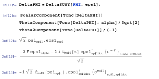
Figure 3.1: Screenshot of a Mathematica session where the variations under a supersymmetric transformation of parameters $(\varepsilon_{1},{\bar{\varepsilon}}_{1})$ of the component fields of a chiral superfield are computed. We refer to the text for more details.

3.4.2 Variation of general superfields

As a second example, we perform the same exercise as in Section 3.4.1 but in the case of general superfields. There is no dedicated function in FeynRules to get the expansion of such superfields in terms of the Grassmann variables so that we have to implement it directly in the Mathematica session. In our example, we consider a general superfield represented by the symbol Phi and use the ncc environment presented in Section 3.3.1 to facilitate its implementation,

  Phi = z + ncc[theta, xi] + ncc[thetabar, zetabar] + ncc[theta, theta] F +
    ncc[thetabar, thetabar] G + ncc[theta, si[mu], thetabar]  v[mu] +
     ncc[thetabar, thetabar] ncc[theta, omega] +
     ncc[theta, theta] ncc[thetabar, rhobar] +
     ncc[theta, theta] ncc[thetabar, thetabar] d

The names and symbols related to the component fields follow those of Eq. (2.3.8), and the list M$ClassesDeclaration accordingly contains

  V[1] == {ClassName -> v, SelfConjugate->True}
  W[1] == {ClassName->zeta,  Chirality->Left, SelfConjugate->False}
  W[2] == {ClassName->xi,    Chirality->Left, SelfConjugate->False}
  W[3] == {ClassName->omega, Chirality->Left, SelfConjugate->False}
  W[4] == {ClassName->rho,   Chirality->Left, SelfConjugate->False}
  S[1] == {ClassName->z, SelfConjugate->False}
  S[2] == {ClassName->F, SelfConjugate->False}
  S[3] == {ClassName->G, SelfConjugate->False}
  S[4] == {ClassName->d, SelfConjugate->False}

The variation of the general superfield under a supersymmetric transformation of parameters $(\varepsilon,{\bar{\varepsilon}})$ is computed as in the previous section,

  DeltaPhi = DeltaSUSY[ Phi , eps1 ]

Extracting the nine component fields by means of the XXXXComponent[DeltaPhi] commands, one gets the textbook expressions

$$\begin{split}\delta z=&\ \varepsilon\!\cdot\!\xi+{\bar{\varepsilon}}\!\cdot\!{\bar{\zeta}}\ ,\\ \delta\xi_{\alpha}=&\ 2f\varepsilon_{\alpha}+\big{(}\sigma^{\mu}{\bar{\varepsilon}}\big{)}_{\alpha}\big{(}v_{\mu}-i\partial_{\mu}z\big{)}\ ,\\ \delta{\bar{\zeta}}^{\dot{\alpha}}=&\ 2g{\bar{\varepsilon}}^{\dot{\alpha}}-\big{(}{\bar{\sigma}}^{\mu}\varepsilon\big{)}^{\dot{\alpha}}\big{(}v_{\mu}+i\partial_{\mu}z\big{)}\ ,\\ \delta v_{\mu}=&\ -\frac{i}{2}\varepsilon\!\cdot\!\partial_{\mu}\xi-\varepsilon\sigma_{\nu\mu}\partial^{\nu}\xi+\frac{i}{2}{\bar{\varepsilon}}\!\cdot\!\partial_{\mu}{\bar{\zeta}}-{\bar{\varepsilon}}{\bar{\sigma}}_{\nu\mu}\partial^{\nu}{\bar{\zeta}}+\omega\sigma_{\mu}{\bar{\varepsilon}}+\varepsilon\sigma_{\mu}{\bar{\rho}}\ ,\\ \delta f=&\ \frac{i}{2}\partial_{\mu}\xi\sigma^{\mu}{\bar{\varepsilon}}+{\bar{\varepsilon}}\!\cdot\!{\bar{\rho}}\ ,\\ \delta g=&\ -\frac{i}{2}\varepsilon\sigma^{\mu}\partial_{\mu}{\bar{\zeta}}+\varepsilon\!\cdot\!\omega\ ,\\ \delta\omega_{\alpha}=&\ -i\big{(}\sigma^{\mu}{\bar{\varepsilon}}\big{)}_{\alpha}\partial_{\mu}g+\frac{i}{2}\varepsilon_{\alpha}\partial_{\mu}v^{\mu}-\frac{i}{2}\big{(}\sigma^{\mu\nu}\varepsilon\big{)}_{\alpha}\ F^{0}_{\mu\nu}+2\varepsilon_{\alpha}d\ ,\\ \delta{\bar{\rho}}_{\dot{\alpha}}=&\ i\big{(}\varepsilon\sigma^{\mu}\big{)}_{\dot{\alpha}}\partial_{\mu}f-\frac{i}{2}{\bar{\varepsilon}}_{\dot{\alpha}}\partial_{\mu}v^{\mu}-\frac{i}{2}\big{(}{\bar{\varepsilon}}\sigma^{\mu\nu}\big{)}_{\dot{\alpha}}F^{0}_{\mu\nu}+2{\bar{\varepsilon}}_{\dot{\alpha}}d\ ,\\ \delta d=&\ \frac{i}{2}\partial_{\mu}\omega\sigma^{\mu}{\bar{\varepsilon}}-\frac{i}{2}\varepsilon\sigma^{\mu}\partial_{\mu}{\bar{\rho}}\ ,=\frac{i}{2}\partial_{\mu}\big{[}\omega\sigma^{\mu}{\bar{\varepsilon}}-\frac{i}{2}\varepsilon\sigma^{\mu}{\bar{\rho}}\big{]}\ ,\end{split}$$ (3.4.2)

where $F^{0}_{\mu\nu}$ is the derivative part of the field strength tensor,

$$F^{0}_{\mu\nu}=\partial_{\mu}v_{\nu}-\partial_{\nu}v_{\mu}\ .$$ (3.4.3)

The variation of the $D$-term proves the statement that the highest-order component field of a general superfield is a good candidate for a supersymmetric Lagrangian (see Section 2.4) since it transforms as a total derivative under supersymmetric transformations.

3.4.3 Vector superfields in the Wess-Zumino gauge

In this section, we apply the results of the previous section to the general vector superfield of Eq. (2.3.17), considering only the non-abelian case since the abelian limit can be easily derived. Switching to notations and normalization conventions of Section 2.3.4, the variations of the component fields are directly read from Eq. (3.4.2). Adopting the Wess-Zumino gauge where the component fields $C^{a}$, $(\chi^{a},{\bar{\chi}}^{a})$, $f^{a}$ and $g^{a}$ vanish, one observes that these five fields transform as

$$\begin{split}C^{a}=0\to&\ C^{a\prime}=C^{a}+i\varepsilon\!\cdot\!\chi^{a}+i{\bar{\varepsilon}}\!\cdot\!{\bar{\chi}}^{a}=0\ ,\\ \chi^{a}_{\alpha}=0\to&\ \chi^{a\prime}_{\alpha}=\chi^{a}_{\alpha}+f^{a}\varepsilon_{\alpha}-i\big{(}\sigma^{\mu}{\bar{\varepsilon}}\big{)}_{\alpha}\big{(}v^{a}_{\mu}-i\partial_{\mu}C^{a}\big{)}=-i\big{(}\sigma^{\mu}{\bar{\varepsilon}}\big{)}_{\alpha}v_{\mu}^{a}\ ,\\ {\bar{\chi}}^{a{\dot{\alpha}}}=0\to&\ {\bar{\chi}}^{a\prime{\dot{\alpha}}}={\bar{\chi}}^{a{\dot{\alpha}}}+f{a^{\dagger}}{\bar{\varepsilon}}^{\dot{\alpha}}-i\big{(}{\bar{\sigma}}^{\mu}\varepsilon\big{)}^{\dot{\alpha}}\big{(}v^{a}_{\mu}+i\partial_{\mu}C^{a}\big{)}=-i\big{(}{\bar{\sigma}}^{\mu}\varepsilon\big{)}^{\dot{\alpha}}v^{a}_{\mu}\ ,\\ f^{a}=0\to&\ f^{a\prime}=f^{a}+i\partial_{\mu}\chi^{a}\sigma^{\mu}{\bar{\varepsilon}}+2{\bar{\varepsilon}}\!\cdot\!\big{(}{\bar{\lambda}}^{a}-\frac{i}{2}{\bar{\sigma}}^{\mu}\partial_{\mu}\chi^{a}\big{)}=2{\bar{\varepsilon}}\!\cdot\!{\bar{\lambda}}^{a}\ ,\\ f^{a{\dagger}}=0\to&\ f^{a\prime{\dagger}}=f^{a{\dagger}}-i\varepsilon\sigma^{\mu}\partial_{\mu}{\bar{\chi}}^{a}+2\varepsilon\!\cdot\!\big{(}\lambda^{a}-\frac{i}{2}\sigma^{\mu}\partial_{\mu}{\bar{\chi}}^{a}\big{)}=2\varepsilon\!\cdot\!\lambda^{a}\ .\end{split}$$ (3.4.4)

The Wess-Zumino gauge is thus not supersymmetric as not preserved by supersymmetric transformations. In Section 2.3.4, we have also motivated the use of vector superfields in the Wess-Zumino gauge instead of general vector superfield by the argument that the component fields $(\lambda,{\bar{\lambda}})$, $v$ and $D$ are transforming into each other under supersymmetric transformations. This is true according to Eq. (3.4.2) since in the notations of Eq. (2.3.17), we have

$$\begin{split}\lambda^{a}_{\alpha}\to&\ \lambda_{\alpha}^{a\prime}=\lambda^{a}_{\alpha}-i(\sigma^{\mu\nu}\varepsilon)_{\alpha}\ F^{0a}_{\mu\nu}+i\varepsilon_{\alpha}D^{a}\ ,\\ {\bar{\lambda}}^{a}_{\dot{\alpha}}\to&\ {\bar{\lambda}}^{a\prime}_{\dot{\alpha}}={\bar{\lambda}}^{a}_{\dot{\alpha}}+i({\bar{\varepsilon}}{\bar{\sigma}}^{\mu\nu})_{\dot{\alpha}}F^{0a}_{\mu\nu}-i{\bar{\varepsilon}}_{\dot{\alpha}}D^{a}\ ,\\ v_{\mu}^{a}\to&\ v^{a\prime}_{\mu}=v^{a}_{\mu}-i\lambda^{a}\sigma_{\mu}{\bar{\varepsilon}}+i\varepsilon\sigma_{\mu}{\bar{\lambda}}^{a}\ ,\\ D^{a}\to&\ D^{a\prime}=D^{a}+\partial_{\mu}\lambda^{a}\sigma^{\mu}{\bar{\varepsilon}}+\varepsilon\sigma^{\mu}\partial_{\mu}{\bar{\lambda}}^{a}=D^{a}+\partial_{\mu}\big{[}\lambda^{a}\sigma^{\mu}{\bar{\varepsilon}}+\varepsilon\sigma^{\mu}{\bar{\lambda}}^{a}\big{]}\ ,\end{split}$$ (3.4.5)

where $F^{0a}_{\mu\nu}$ denotes the derivative terms of the non-abelian field strength tensor. However, vector superfields are closely related to gauge transformations, and in order to preserve the Wess-Zumino gauge, it is necessary to accompany supersymmetry transformations by gauge transformations. From Eq. (2.4.29), the variation of a vector superfield $\delta_{g}\Phi_{V}^{a}$ under a gauge transformation reads

$$\delta_{g}\Phi_{V}^{a}=-i(\Lambda^{a}-\Lambda^{a{\dagger}})-gf_{bc}{}^{a}\Phi_{V}^{b}(\Lambda^{c}+\Lambda^{c{\dagger}})\ ,$$ (3.4.6)

where $\Lambda$ is the (superfield) transformation parameter. We now use FeynRules to show that fixing

$$\Lambda^{a}=-i\theta\sigma^{\mu}{\bar{\varepsilon}}v^{a}_{\mu}+\theta\!\cdot\!\theta\ {\bar{\varepsilon}}\!\cdot\!{\bar{\lambda}}^{a}\ ,$$ (3.4.7)

allows to restore the Wess-Zumino gauge.

First, we assume that the non-abelian vector superfield $\Phi_{V}$ and its component fields $\lambda$, $v$ and $D$ have been properly declared, as shown in Section 3.1.5 and Section 3.3.3. Moreover, the gauge group associated to $\Phi_{V}$, as well as the related adjoint gauge index and the structure constants $f_{bc}{}^{a}$, must also have been declared following the syntax of Section 3.1.2 and Section 3.1.3. Finally, the coupling constant has to be added to the list of parameters, as presented in Section 3.1.4.

Then, we associate the symbol LAM to the superfield $\Lambda$ of Eq. (3.4.7). Its implementation in FeynRules reads

  LAM[a_] := -I ncc[theta,si[mu],eps1bar] V[mu, a] +
     ncc[theta,theta] ncc[eps1bar,lambdabar[a]];

where as in the beginning of this section, we employ the predefined spinor eps1 for the transformation parameters and the ncc environment to handle the canonical form of the superspace expressions. The variation under a gauge transformation is finally computed as

  deltag := -I (LAM[a]-HC[LAM[a]]) - g f[b,c,a] PHIV[b] (LAM[c]+HC[LAM[c]])

assuming that the vector superfield, the structure constants and the coupling strength related the gauge group are represented by the symbols PHIV, f[a,b,c] and g. Expanding this expression in terms of the Grassmann coordinates,

  GrassmannExpand[deltag]

one gets

$$\begin{split}\delta_{g}\Phi_{V}^{a}=&\ -\theta\sigma^{\mu}{\bar{\varepsilon}}v_{\mu}^{a}+{\bar{\theta}}{\bar{\sigma}}^{\mu}\varepsilon v_{\mu}^{a}-i\theta\!\cdot\!\theta{\bar{\lambda}}^{a}\!\cdot\!{\bar{\varepsilon}}+i{\bar{\theta}}\!\cdot\!{\bar{\theta}}\lambda^{a}\!\cdot\!\varepsilon-gf_{bc}{}^{a}{\bar{\theta}}\!\cdot\!{\bar{\theta}}\theta\sigma^{\mu\nu}\varepsilon v_{\mu}^{b}v_{\nu}^{c}\\ &\quad+igf_{bc}{}^{a}\theta\!\cdot\!\theta{\bar{\theta}}{\bar{\sigma}}^{\mu\nu}{\bar{\varepsilon}}v_{\mu}^{b}v_{\nu}^{c}+\frac{1}{2}gf_{bc}{}^{a}v_{\mu}^{c}\big{[}\varepsilon\sigma^{\mu}{\bar{\lambda}}^{b}+\lambda^{b}\sigma^{\mu}{\bar{\varepsilon}}\big{]}\end{split}$$ (3.4.8)

Merging this result with the normalization of the fields introduced in Eq. (2.3.17) and the variations of Eq. (3.4.4) and Eq. (3.4.5), one obtains

$$C^{a}=C^{a\prime}=\chi^{a}_{\alpha}=\chi^{a\prime}_{\alpha}={\bar{\chi}}^{a{\dot{\alpha}}}={\bar{\chi}}^{a\prime{\dot{\alpha}}}=f^{a}=f^{a\prime}=f^{a{\dagger}}=f^{a\prime{\dagger}}=0\ ,$$ (3.4.9)

which effectively restores the Wess-Zumino gauge. In addition, the variation of the components of the vector supermultiplet of Eq. (3.4.5) are now covariant with respect to gauge transformations,

$$\begin{split}\lambda^{a}_{\alpha}\to&\ \lambda_{\alpha}^{a\prime}=\lambda^{a}_{\alpha}-i(\sigma^{\mu\nu}\varepsilon)_{\alpha}\ F^{a}_{\mu\nu}+i\varepsilon_{\alpha}D^{a}\ ,\\ {\bar{\lambda}}^{a}_{\dot{\alpha}}\to&\ {\bar{\lambda}}^{a\prime}_{\dot{\alpha}}={\bar{\lambda}}^{a}_{\dot{\alpha}}+i({\bar{\varepsilon}}{\bar{\sigma}}^{\mu\nu})_{\dot{\alpha}}F^{a}_{\mu\nu}-i{\bar{\varepsilon}}_{\dot{\alpha}}D^{a}\ ,\\ v_{\mu}^{a}\to&\ v^{a\prime}_{\mu}=v^{a}_{\mu}-i\lambda^{a}\sigma_{\mu}{\bar{\varepsilon}}+i\varepsilon\sigma_{\mu}{\bar{\lambda}}^{a}\ ,\\ D^{a}\to&\ D^{a\prime}=D^{a}+D_{\mu}\big{[}\lambda^{a}\sigma^{\mu}{\bar{\varepsilon}}+\varepsilon\sigma^{\mu}{\bar{\lambda}}^{a}\big{]}\ ,\end{split}$$ (3.4.10)

where $F^{a}_{\mu\nu}$ is the standard non-abelian field strength tensor and $D_{\mu}\lambda^{a}$ and $D_{\mu}{\bar{\lambda}}^{a}$ the covariant derivatives in the adjoint representation given in Eq. (2.4.34).

We achieve this section by considering the variations of the chiral superfield of Section 3.4.1 under a joint supersymmetric and gauge transformation. At the infinitesimal level, Eq. (2.4.45) reads

$$\delta_{g}\Phi=-2ig\Lambda^{a}T_{a}\Phi\ .$$ (3.4.11)

This can be implemented in FeynRules as

  dgphi[i_] := -2 I g LAM[a] T[a,i,j] PHI[j]

where we assume that the superfield $\Phi$ lies in a representation of the gauge group spanned by the matrices $T_{a}$. Extracting the scalar, fermionic and auxiliary coefficients of the chiral superfield $\delta_{g}\Phi$ by means of the functions XXXXComponent and introducing appropriate normalization factors, one gets

$$\begin{split}\delta_{g}z=&\ 0\ ,\\ \delta_{g}\psi_{\alpha}=&\ -\sqrt{2}g\big{(}\sigma^{\mu}{\bar{\varepsilon}}\big{)}_{\alpha}v_{\mu}^{a}\big{(}T_{a}z\big{)}\ ,\\ \delta_{g}F=&\ 2ig\big{(}T_{a}z\big{)}{\bar{\lambda}}^{a}\!\cdot\!{\bar{\varepsilon}}-\sqrt{2}g\big{(}T_{a}\psi\big{)}\sigma^{\mu}{\bar{\varepsilon}}v_{\mu}^{a}\ .\end{split}$$ (3.4.12)

Combining these results with those of Eq. (3.4.1), the variations of the component fields of a chiral superfield under the composition of a gauge and a supersymmetric transformation are now gauge covariant,

$$\begin{split}\delta_{\varepsilon}z=&\ \sqrt{2}\varepsilon\!\cdot\!\psi\ ,\\ \delta_{\varepsilon}\psi_{\alpha}=&\ -\sqrt{2}\varepsilon_{\alpha}F-i\sqrt{2}\big{(}\sigma^{\mu}{\bar{\varepsilon}}\big{)}_{\alpha}D_{\mu}z\ ,\\ \delta_{\varepsilon}F=&\ -i\sqrt{2}D_{\mu}\big{[}\psi\sigma^{\mu}{\bar{\varepsilon}}\big{]}+2ig\big{(}T_{a}z\big{)}{\bar{\lambda}}^{a}\!\cdot\!{\bar{\varepsilon}}\ ,\end{split}$$ (3.4.13)

which recovers well-known textbook results. We recall that the covariant derivatives of the scalar and fermionic fields, automatically expanded in FeynRules, are given by Eq. (2.4.58).

3.5 Non-renormalizable supersymmetric model building

In this section, we give an additional example to illustrate the power of FeynRules for superspace calculations by computing the Kähler potential of Eq. (2.4.6). We start with the declaration of two sets of indices, denoted by II and JS, related to chiral and antichiral superfields, respectively,

  IndexRange[Index[II]] = Range[12];    IndexRange[Index[JS]] = Range[12];

where the ranges of these indices are arbitrary since irrelevant for the following. We then include in M$ClassesDescription two sets of component fields associated with these indices,

  W[1] == {ClassName->psiL, Chirality->Left, SelfConjugate->False,
    Indices->{Index[II]}}
  W[2] == {ClassName->psiR, Chirality->Left, SelfConjugate->False,
    Indices->{Index[JS]}}
  S[1] == {ClassName->phiL, SelfConjugate->False, Indices->{Index[II]}}
  S[2] == {ClassName->phiR, SelfConjugate->False, Indices->{Index[JS]}}
  S[3] == {ClassName->FL, SelfConjugate->False, Unphysical->True,
    Indices->{Index[II]}}
  S[4] == {ClassName->FR, SelfConjugate->False, Unphysical->True,
    Indices->{Index[JS]}}

and we omit the declaration of the corresponding chiral and antichiral superfields $\Phi^{i}$ and $\Phi^{\dagger}_{i^{\ast}}$ as not necessary for our scope. Since these fields are all members of chiral (and not antichiral) supermultiplets, the Hermitian conjugate of the fields carrying a starry index JS have to be further used.

The Kähler potential is defined from the left-handed and right-handed chiral superfields $W^{I}(\Phi)$ and $W_{I}(\Phi^{\dagger})$ of Eq. (2.4.5). These two superfields are declared in the M$Superfields list,

  CSF[1] == { ClassName->WISF, Chirality->Left, Weyl->psWL, Scalar->phWL,
    Auxiliary->FWL}
  CSF[2] == { ClassName->WISFbar, Chirality->Right,  Weyl->psWR, Scalar->phWR,
    Auxiliary->FWR}

where their component fields have been declared in M$ClassesDescription,

  W[3] == {ClassName->psWL, Chirality->Left,  SelfConjugate->False}
  W[4] == {ClassName->psWR, Chirality->Right, SelfConjugate->False}
  S[5] == {ClassName->phWL, SelfConjugate->False}
  S[6] == {ClassName->phWR, SelfConjugate->False}
  S[7] == {ClassName->FWL,  SelfConjugate->False, Unphysical->True}
  S[8] == {ClassName->FWR,  SelfConjugate->False, Unphysical->True}

To get the correct expansion of the Kähler potential in terms of the Grassmann variables, these fields have to be further replaced by the relevant expressions. These replacement rules require the declarations as parameters of the functions of the scalar fields $W^{I}$ and $W_{I}$ and their derivatives. They are included in the M$Parameters list,

  WI   == { TeX->Superscript[W,"I"] }
  DWI  == { TeX->Superscript[W,"I"], Indices->{Index[II]} }
  DDWI == { TeX->Superscript[W,"I"], Indices->{Index[II], Index[II]}}
  WIbar   == { TeX->Subscript[W,"I"] }
  DWIbar  == { TeX->Subscript[W,"I"], Indices->{Index[JS]} }
  DDWIbar == { TeX->Subscript[W,"I"], Indices->{Index[JS], Index[JS]}}

Consequently, the replacement rules for the component fields associated with the chiral superfield $W^{I}$, being implemented following a standard Mathematica syntax, read

  rules := {
    del[del[phWL,mu_],mu_] :> Module[{ii,jj}, DDWI[ii,jj] del[phiL[ii],mu] *
      del[phiL[jj], mu] + DWI[ii] del[del[phiL[ii],mu],mu]],
    del[phWL,mu_] :> Module[{ii}, DWI[ii] del[ phiL[ii], mu]],
    phWL -> WI,
    del[psWL[sp_], mu_] :> Module[{ii,jj}, del[psiL[sp,ii],mu] DWI[ii] +
      psiL[sp,ii] del[phiL[jj],mu] DDWI[ii,jj]],
    psWL[sp_] :> Module[{ii}, psiL[sp,ii] DWI[ii]],
    FWL :> Module[{ii,jj}, FL[ii] DWI[ii] + 1/2 ncc[psiL[ii],psiL[jj]] *
      DDWI[ii,jj]]
  }

The rules associated with the antichiral superfield $W_{I}$ being similar, they are omitted from the present document for brevity.

We are now ready to compute the Kähler potential, by simply issuing in a Mathematica session

  kahler = GrassmannExpand[WISFbar WISF];
  kahler = Tonc[kahler]/.rules;
  kahler = Expand[kahler];

The first command above gives a rather long expression not yet depending on the Kähler potential and its derivatives. We choose to get back to the nc environment by means of the Tonc function (see Section 3.3.1) before applying the replacement rules in the second command. This allows to avoid the Mathematica Dot environment, explicitly removed by the Tonc method, which could lead to expansion issues when replacing the fermionic components of the $W_{I}$ and $W^{I}$ superfields by their correct expressions.

In order to map the products of derivatives of the (scalar) function $W^{I}$ and $W_{I}$, a second set of standard Mathematica replacement rules has to be applied on the result,

  {WI WIbar->K[{},{}], WIbar*DDWI[i__]->K[{i},{}], WIbar*DWI[i__]->K[{i},{}],
  WI*DDWIbar[i__]->K[{},{i}], WI*DWIbar[i__]->K[{},{i}],
  DDWIbar[j__]*DDWI[i__]->K[{i},{j}], DWIbar[j__]*DDWI[i__]->K[{i},{j}],
  DDWIbar[j__]*DWI[i__]->K[{i},{j}], DWIbar[j__]*DWI[i__]->K[{i},{j}]}

In the commands above, we have introduced a function K taking two lists as arguments, the first one being related to derivation operations with respect to the chiral fields and the second one to those associated with the antichiral fields. It can be checked that the results match the one presented in Eq. (2.4.6), after having expanded all the covariant derivatives included in this equation as given by Eq. (2.4.10) and employed the definitions of Eq. (2.4.7). Moreover, the Mathematica output readability can be improved by adding the formatting rule

  Format[K[{ii___},{jj___}]]:=Subsuperscript[K, StringJoin@@(ToString/@{ii}),
    StringJoin@@(ToString/@{jj})]

Chapter 4 Supersymmetry breaking

Since not a single superpartner with the mass of its Standard Model counterpart has been observed up to now, supersymmetry must be broken. We present in this chapter the main features of supersymmetry breaking and detail the most studied mechanisms.

4.1 Supersymmetry breaking: general features

4.1.1 Motivations for softly broken supersymmetric theories

For many years, the Standard Model of particle physics [1, 2, 3, 4, 5, 6, 7, 8, 9, 10] has passed impressively all experimental tests. Only the mechanism of electroweak symmetry breaking and the one of generation of mass have for a long time remained unsolved questions. Those two issues are however presently addressed by the general-purpose experiments ATLAS and CMS at the LHC, since both experiments have observed a new neutral scalar particle that seems compatible with a Standard-Model-like Higgs boson [11, 12]. However, despite of the success of the Standard Model, many fundamental questions remain unanswered.

One of the most infamous conceptual problem of the Standard Model lies in the non-explained large hierarchy between the electroweak scale and the Planck scale. The latter lying orders of magnitude away from the weak scale, the mass of any fundamental scalar field, and in particular, the one of the new state observed by the ATLAS and CMS experiments, is found to be drastically affected by quantum corrections. Furthermore, many questions arise from the complicated structure of the $SU(3)_{c}\times SU(2)_{L}\times U(1)_{Y}$ Standard Model gauge group. For instance, there is no fundamental reason for the chosen representation of the matter fields and this choice additionally implies the non-unification of the gauge coupling constants at high energies. Moreover, the Standard Model does not provide a mechanism for neutrino oscillations or a candidate particle to account for the presence of dark matter in the universe. As last examples, one can also state that it also does not motivate the non-vanishing cosmological constant, does not provide an explanation for the strong $CP$-problem and does not include gravity.

Over the last decades, large classes of theories have been proposed in order to extend the Standard Model and address one or several of its open issues. Among all these new physics theories, we focus in this work on supersymmetry, a particularly appealing extension of the Standard Model as theoretically well-motivated (see Chapter 2). Supersymmetry is known to solve the hierarchy problem by the introduction of the superpartners of the Standard Model degrees of freedom. Their presence also leads to a modification of the renormalization group equations driving the evolution of the gauge coupling constants between two energy scales, allowing for supersymmetry to tackle the problem of the unification of the gauge couplings at high energies. Many supersymmetric models contain, in addition to gauge symmetries, extra discrete symmetries that typically render the lightest supersymmetric particle stable, which can then be seen as a viable dark matter candidate. Finally, local supersymmetry, also known as supergravity, provides a possible way to include gravity next to the other interactions.

Even if supersymmetry is very attractive both from the theoretical and phenomenological points of view, we have shown in Section 2.2.2 that all the components of a given supermultiplet have the same mass. However, not a single supersymmetric partner of the Standard Model particles has been observed so far, especially at the LHC [42, 43, 179]. In particular, no hint for a scalar electron with a 511 keV mass or for a very light scalar quark of a few MeV has been found. Therefore, supersymmetry cannot be an exact symmetry of nature and building phenomenologically viable supersymmetric models requires to break supersymmetry at low energies. In order to remain a viable solution to the hierarchy problem, this breaking is required to be soft, yielding supersymmetric masses around the TeV scale that are thus reachable at the LHC.

We dedicate the rest of this section to a presentation of the general properties of supersymmetry breaking, while three of the most studied mechanisms implying soft supersymmetry breaking are briefly reviewed in Section 4.2. For all those mechanisms, supersymmetry breaking generally occurs at a higher scale where some organizing relations among the model parameters hold. In contrast, the current particle physics experimental program is designed to probe a much lower scale, the electroweak scale, so that associated phenomenological works require to evolve those parameters down to the electroweak scale. This evolution is controlled by highly coupled differential equations, the supersymmetric renormalization group equations, that we present in Section 4.3.

4.1.2 The Goldstone theorem for supersymmetry

As for any symmetry, supersymmetry is spontaneously broken under the condition that the vacuum state $|\Omega\rangle$ is not invariant under supersymmetry transformations. In other words, the action of the supercharges on the vacuum state obeys to

$$Q_{\alpha}|\Omega\rangle\neq 0\qquad\text{and}\qquad{\bar{Q}}_{\dot{\alpha}}|\Omega\rangle\neq 0\ .$$ (4.1.1)

From the energy operator $P^{0}$ and the superalgebra of Eq. (2.1.37), one can derive a constraint on the energy $E$ of the vacuum state,

$$\begin{split}\langle\Omega|E|\Omega\rangle=&\ \langle\Omega|P^{0}|\Omega\rangle=\frac{1}{4}\Big{\langle}\Omega\Big{|}\big{\{}Q_{1},Q_{1}^{\dagger}\big{\}}+\big{\{}Q_{2},Q_{2}^{\dagger}\big{\}}\Big{|}\Omega\Big{\rangle}\\ =&\ \frac{1}{4}\Big{[}\big{|}\big{|}Q_{1}|\Omega\rangle\big{|}\big{|}+\big{|}\big{|}Q_{2}|\Omega\rangle\big{|}\big{|}+\big{|}\big{|}Q_{1}^{\dagger}|\Omega\rangle\big{|}\big{|}+\big{|}\big{|}Q_{2}^{\dagger}|\Omega\rangle\big{|}\big{|}\Big{]}\neq 0\ ,\end{split}$$ (4.1.2)

so that $E$ is non-vanishing on the basis of Eq. (4.1.1). Moreover, a norm being positively defined, the energy, being equal to the sum of four norms, is thus positive too.

Considering the vacuum state, the Hamiltonian $P^{0}$, as the Lagrangian ${\cal L}$, is reduced to the scalar potential $V$. Therefore, the vacuum expectation value of the potential is positively defined, $\langle V\rangle>0$, as shown in Eq. (4.1.2) and the scalar potential gets a non-trivial minimum. To investigate under which conditions this minimum is reached, we start from the solutions of the equations of motion for the auxiliary fields given in Eq. (2.4.67). In the limit of a renormalizable theory, these solutions become, after accounting for Eq. (2.4.68) and the properties of the Kähler metric of Eq. (2.4.8),

$$F^{i}=W^{\star i}\ ,\qquad F^{\dagger}_{i}=W_{i}\qquad\text{and}\qquad D^{a}=g\phi^{\dagger}_{i}\big{(}T^{a}\phi\big{)}^{i}\ .$$ (4.1.3)

In our theoretical setup, we construct a generic supersymmetric theory describing the dynamics of a set of chiral superfield $\{\Phi^{i}\}$ in interaction. The scalar, fermionic and auxiliary component fields of these superfields are denoted by $\phi^{i}$, $\psi^{i}$ and $F^{i}$, respectively, as in Chapter 2. Moreover, we also recall our conventions for the shorthand notations employed for the first-order derivatives of the superpotential $W$ (and those of the Hermitian conjugate function $W^{\star}$) that appear in Eq. (4.1.3),

$$W_{i}\equiv\frac{\partial W(\phi)}{\partial\phi^{i}}\qquad\text{and}\qquad W^{\star i}\equiv\frac{\partial W^{\star}(\phi^{\dagger})}{\partial\phi^{\dagger}_{i}}\ .$$ (4.1.4)

Finally, the matrices $T_{a}$, on which depend the solutions of the equations of motion for the $D$-fields, are representation matrices of the gauge group associated with the representation in which the scalar fields $\phi^{i}$ and $\phi^{\dagger}_{i}$ lie, and as usual, the coupling constant of the gauge group is denoted by $g$. Inserting Eq. (4.1.3) in the Lagrangian of Eq. (2.4.71), the scalar potential $V$ can be rewritten exclusively in terms of the auxiliary fields,

$$V=F^{i}F^{\dagger}_{i}+\frac{1}{2}D^{a}D_{a}\ .$$ (4.1.5)

As stated above, the vacuum expectation value of the scalar potential is positive, $\langle V\rangle>0$. From the results of Eq. (4.1.5), supersymmetry is thus broken in the case at least one of the auxiliary fields gets a non-vanishing vacuum expectation value.

The minimization conditions for the scalar potential imply that the first-order derivatives of $V$ with respect to the scalar fields vanish at the minimum,

$$0=\left\langle\frac{\partial V}{\partial\phi_{j}}\right\rangle=\left\langle F^{i}\frac{\partial F^{\dagger}_{i}}{\partial\phi^{j}}+D^{a}\frac{\partial D^{a}}{\partial\phi^{j}}\right\rangle=\left\langle F^{i}W_{ij}+gD^{a}(\phi^{\dagger}T_{a})_{j}\right\rangle\qquad\forall j\ ,$$ (4.1.6)

where the equalities are derived after inserting the solutions of the equations of motion for the auxiliary fields of Eq. (4.1.3) in the expression of the scalar potential of Eq. (4.1.5) . Additional information can be obtained from the fact that superpotential is a gauge-invariant quantity. Consequently, its variation under a gauge transformation vanishes,

$$0=\delta_{\omega}W^{\star}=W^{\star i}\delta_{\omega}\phi^{\dagger}_{i}=F^{i}\Big{[}ig\omega^{a}(\phi^{\dagger}T_{a})_{i}\Big{]}\ ,$$ (4.1.7)

where $\omega^{a}$ are the transformation parameters. In order to derive this last result, we have used the equation of motions for the auxiliary $F$-field and we recall that, at the infinitesimal level, the scalar fields transform as

$$\phi^{i}\to\phi^{i}-ig\omega^{a}\big{(}T_{a}\phi\big{)}^{i}\qquad\text{and}\qquad\phi^{\dagger}_{i}\to\phi^{\dagger}_{i}+ig\omega^{a}\big{(}\phi^{\dagger}T_{a}\big{)}_{i}\ .$$ (4.1.8)

The two conditions of Eq. (4.1.6) and Eq. (4.1.7) can be collected into a single matrix equation characterizing the vacuum state,

$$\boxed{\begin{pmatrix}\langle W_{ij}\rangle&\langle g\phi_{k}^{\dagger}(T_{a})^{k}{}_{j}\rangle\\ \langle g\phi_{k}^{\dagger}(T_{a})^{k}{}_{i}\rangle&0\end{pmatrix}\begin{pmatrix}\langle F^{i}\rangle\\ \langle D^{a}\rangle\end{pmatrix}=\begin{pmatrix}0\\ 0\end{pmatrix}\ .}$$ (4.1.9)

We now investigate the fermionic sector, and in particular the mass matrices resulting from the spontaneous breaking of supersymmetry. The interaction terms of the Lagrangian yielding fermionic mass terms, that we denote by ${\cal L}_{\rm int}^{\psi}$, can be extracted from Eq. (2.4.71),

$${\cal L}_{\rm int}^{\psi}=-\frac{1}{2}W_{ij}\psi^{i}\!\cdot\!\psi^{j}-\sqrt{2}ig\phi^{\dagger}_{i}(T_{a})^{i}{}_{j}\psi^{j}\!\cdot\!\lambda^{a}+{\rm h.c.}\ .$$ (4.1.10)

Shifting the scalar fields with respect to their vacuum expectation values then generates the mass terms

$${\cal L}_{\rm mass}^{\psi}=-\frac{1}{2}\begin{pmatrix}\psi^{j}&\sqrt{2}i\lambda^{a}\end{pmatrix}^{\alpha}\begin{pmatrix}\langle W_{ij}\rangle&\langle g\phi_{k}^{\dagger}(T_{b})^{k}{}_{j}\rangle\\ \langle g\phi_{k}^{\dagger}(T_{a})^{k}{}_{i}\rangle&0\end{pmatrix}\begin{pmatrix}\psi^{i}\\ \sqrt{2}i\lambda^{b}\end{pmatrix}_{\alpha}+{\rm h.c.}\ .$$ (4.1.11)

Using the minimization conditions of Eq. (4.1.9), we observe that the fermionic field defined by

$$\boxed{|\psi_{G}\rangle=\frac{\sqrt{2}}{2}\langle F_{i}^{\dagger}\rangle\ |\psi^{i}\rangle+\frac{i}{2}\langle D^{a}\rangle\ |\lambda_{a}\rangle}$$ (4.1.12)

is massless.

The prediction of the existence of such a massless field, dubbed a goldstino, consists of the Goldstone theorem for supersymmetry. When supersymmetry is spontaneously broken, the scalar potential is minimum for a configuration in which at least one of the auxiliary fields gets a non-vanishing vacuum expectation value $\langle F^{i}\rangle$ or $\langle D^{a}\rangle$ and the particle spectrum consequently contains a massless fermionic state $\psi_{G}$ defined by Eq. (4.1.12) [39, 94].

4.1.3 Properties of the goldstino field

As explained in the previous section, spontaneous supersymmetry breaking predicts the existence of a massless (Majorana) fermion, the goldstino. The interactions of such a field with the rest of the particle spectrum can be derived from the conservation of the Nœther current. We recall that the current is defined from the variation of the Lagrangian ${\cal L}$ under a supersymmetry transformation, as shown in Eq. (2.1.5),

$$\delta_{\varepsilon}{\cal L}=\partial_{\mu}K^{\mu}=\partial_{\mu}\bigg{[}{\partial{\cal L}\over\partial\big{(}\partial_{\mu}X\big{)}}\delta_{\varepsilon}X\bigg{]}\ ,$$ (4.1.13)

where the quantity $K^{\mu}$ is obtained after directly varying the fields appearing in the Lagrangian and where the Majorana fermion $(\varepsilon,{\bar{\varepsilon}})$ denotes the transformation parameters. As in Chapter 2, the second equality is obtained on the basis of Euler-Lagrange equations, a sum over all the fields $X$ of the theory being understood. Consequently, the supercurrent $(J^{\mu},{\bar{J}}^{\mu})$, defined as

$$\varepsilon\!\cdot\!J^{\mu}+{\bar{\varepsilon}}\!\cdot\!{\bar{J}}^{\mu}={\partial{\cal L}\over\partial\big{(}\partial_{\mu}X\big{)}}\delta_{\varepsilon}X-K^{\mu}\ ,$$ (4.1.14)

is a conserved quantity.

In Chapter 2, we have derived supersymmetric Lagrangians both in terms of superfields and component fields and have shown that, in terms of superfields, a supersymmetric Lagrangian can generically be written as a sum of five terms,

$${\cal L}=\Big{[}\Phi_{i}^{\dagger}e^{-2gV}\Phi^{i}\Big{]}_{\theta^{2}{\bar{\theta}}^{2}}+\frac{1}{16g^{2}}\Big{[}W^{\alpha}_{a}W^{a}_{\alpha}\Big{]}_{\theta^{2}}+\frac{1}{16g^{2}}\Big{[}{\overline{W}}_{\dot{\alpha}}^{a}{\overline{W}}_{a}^{\dot{\alpha}}\Big{]}_{{\bar{\theta}}^{2}}+\Big{[}W(\Phi)\Big{]}_{\theta^{2}}+\Big{[}W^{\star}(\Phi^{\dagger})\Big{]}_{{\bar{\theta}}^{2}}\ ,$$ (4.1.15)

where the subscripts indicate which coefficients of the expansion in terms of the Grassmann variables have to be selected. We recall that in this expression, the (generic) coupling constant of the gauge group is denoted by $g$ and we consider a theory describing the dynamics of a set of chiral superfields $\{\Phi^{i}\}$. We have also associated with the gauge group of the theory a set of vector superfields $\{V^{a}\}$ lying in its adjoint representation. The related Lagrangian terms, i.e., the second and third terms of Eq. (4.1.15), rely on the superfield strength tensors built from the vector superfields $V^{a}$, the spinorial superfields $W_{\alpha}^{a}$ and ${\overline{W}}_{\dot{\alpha}}^{a}$ defined by Eq. (2.4.30).

From the variation laws of the different component fields of a general superfield, as collected in Eq. (3.4.2), as well as from those of a chiral superfield shown in Eq. (3.4.1), the variation of the Lagrangian above under a supersymmetry transformation of parameters $(\varepsilon,{\bar{\varepsilon}})$ reads

$$\begin{split}\delta_{\varepsilon}{\cal L}=&\ -\frac{i}{2}\varepsilon\sigma^{\mu}\partial_{\mu}\Big{[}\Phi_{i}^{\dagger}e^{-2gV}\Phi^{i}\Big{]}_{\theta^{2}{\bar{\theta}}}-\frac{i}{2}{\bar{\varepsilon}}{\bar{\sigma}}^{\mu}\partial_{\mu}\Big{[}\Phi_{i}^{\dagger}e^{-2gV}\Phi^{i}\Big{]}_{\theta{\bar{\theta}}^{2}}\\ &\ -i\varepsilon\sigma^{\mu}\partial_{\mu}\Big{[}W^{\star}(\Phi^{\dagger})+\frac{1}{16g^{2}}{\overline{W}}_{\dot{\alpha}}^{a}{\overline{W}}_{a}^{\dot{\alpha}}\Big{]}_{\bar{\theta}}-i{\bar{\varepsilon}}{\bar{\sigma}}^{\mu}\partial_{\mu}\Big{[}W(\Phi)+\frac{1}{16g^{2}}W^{\alpha}_{a}W^{a}_{\alpha}\Big{]}_{\theta}\ .\end{split}$$ (4.1.16)

Expanding the superfields in terms of their component fields and selecting the proper coefficients of the series in the Grassmann variables, one finds, after inserting the solutions of the equations of motion for the auxiliary fields,

$$\begin{split}\delta_{\varepsilon}{\cal L}=&\ \varepsilon\!\cdot\!\partial_{\mu}\bigg{[}\frac{\sqrt{2}}{2}D_{\nu}\phi^{\dagger}_{i}\sigma^{\mu}{\bar{\sigma}}^{\nu}\psi^{i}-\frac{\sqrt{2}i}{2}\sigma^{\mu}{\bar{\psi}}_{i}W^{\star i}-\frac{1}{2}g\phi_{i}^{\dagger}\big{(}T_{a}\phi\big{)}^{i}\sigma^{\mu}{\bar{\lambda}}^{a}-\frac{i}{4}\sigma^{\mu}{\bar{\sigma}}^{\nu}\sigma^{\rho}{\bar{\lambda}}_{a}F^{a}_{\nu\rho}\\ &\ -\frac{\sqrt{2}}{4}\partial_{\nu}\big{[}\phi^{\dagger}_{i}\sigma^{\mu}{\bar{\sigma}}^{\nu}\psi^{i}\big{]}\bigg{]}+{\bar{\varepsilon}}\!\cdot\!\partial_{\mu}\bigg{[}\frac{\sqrt{2}}{2}D_{\nu}\phi^{i}{\bar{\sigma}}^{\mu}\sigma^{\nu}{\bar{\psi}}_{i}-\frac{\sqrt{2}i}{2}{\bar{\sigma}}^{\mu}\psi^{i}W_{i}\\ &\ +\frac{1}{2}g\big{(}\phi^{\dagger}T_{a}\big{)}_{i}\phi^{i}{\bar{\sigma}}^{\mu}\lambda^{a}-\frac{i}{4}{\bar{\sigma}}^{\mu}\sigma^{\nu}{\bar{\sigma}}^{\rho}\lambda_{a}F^{a}_{\nu\rho}-\frac{\sqrt{2}}{4}\partial_{\nu}\big{[}\phi^{i}{\bar{\sigma}}^{\mu}\sigma^{\nu}{\bar{\psi}}_{i}\big{]}\bigg{]}\ .\end{split}$$ (4.1.17)

To compute this last result, we have performed two integrations by parts (explicitly including all total derivatives) and introduced the gauge covariant derivatives of the scalar fields given in Eq. (2.4.64). One derives from this expression the quantity $K^{\mu}$ of Eq. (4.1.13) and Eq. (4.1.14),

$$\begin{split}K^{\mu}_{\alpha}=&\ \frac{\sqrt{2}}{2}D_{\nu}\phi^{\dagger}_{i}\big{(}\sigma^{\mu}{\bar{\sigma}}^{\nu}\psi^{i}\big{)}_{\alpha}-\frac{\sqrt{2}i}{2}\big{(}\sigma^{\mu}{\bar{\psi}}_{i}\big{)}_{\alpha}W^{\star i}-\frac{1}{2}g\phi_{i}^{\dagger}\big{(}T_{a}\phi\big{)}^{i}\big{(}\sigma^{\mu}{\bar{\lambda}}^{a}\big{)}_{\alpha}\\ &\ -\frac{i}{4}\big{(}\sigma^{\mu}{\bar{\sigma}}^{\nu}\sigma^{\rho}{\bar{\lambda}}_{a}\big{)}_{\alpha}F^{a}_{\nu\rho}-\frac{\sqrt{2}}{4}\partial_{\nu}\Big{[}\phi^{\dagger}_{i}\big{(}\sigma^{\mu}{\bar{\sigma}}^{\nu}\psi^{i}\big{)}_{\alpha}\Big{]}\ .\end{split}$$ (4.1.18)

To achieve the calculation of the supercurrent, it is also necessary to compute the first term of the right-hand side of Eq. (4.1.14). To this aim, it is enough to select the derivative terms of the supersymmetric Lagrangian of Eq. (2.4.72),

$$\begin{split}{\cal L}=&\ -\frac{1}{4}\partial_{\mu}\big{(}\phi^{\dagger}_{i}\partial^{\mu}\phi^{i}+\partial^{\mu}\phi^{\dagger}_{i}\phi^{i}\big{)}+D^{\mu}\phi^{\dagger}_{i}D_{\mu}\phi^{i}+\frac{i}{2}\Big{[}\psi^{i}\sigma^{\mu}D_{\mu}{\bar{\psi}}_{i}-D_{\mu}\psi^{i}\sigma^{\mu}{\bar{\psi}}_{i}\big{]}\\ &\ -\frac{1}{4}F^{a}_{\mu\nu}F_{a}^{\mu\nu}+\frac{i}{2}\Big{[}\lambda^{a}\sigma^{\mu}D_{\mu}{\bar{\lambda}}_{a}-D_{\mu}\lambda^{a}\sigma^{\mu}{\bar{\lambda}}_{a}\Big{]}\ ,\end{split}$$ (4.1.19)

and perform the derivation of this expression with respect to the first-order derivatives of the fields. We have included in this Lagrangian the total derivative that was originally originally present (see, e.g., Eq.(2.4.61)) and then omitted in the computations of Chapter 2. From the variations of the fields computed in Eq. (3.4.12) and Eq. (3.4.13), one gets, after inserting again the solutions of the equations of motion for the auxiliary fields,

$$\begin{split}{\partial{\cal L}\over\partial\big{(}\partial_{\mu}X\big{)}}\delta X=&\ \varepsilon\!\cdot\!\Big{[}\sqrt{2}D_{\mu}\phi_{i}^{\dagger}\psi^{i}-\frac{\sqrt{2}}{4}\partial^{\mu}(\phi_{i}^{\dagger}\psi^{i})+\frac{\sqrt{2}i}{2}\sigma^{\mu}{\bar{\psi}}_{i}W^{\star i}+\frac{\sqrt{2}}{2}D_{\nu}\phi_{i}^{\dagger}\sigma^{\nu}{\bar{\sigma}}^{\mu}\psi^{i}\\ &\ -i\sigma_{\nu}{\bar{\lambda}}^{a}F_{a}^{\mu\nu}+\frac{1}{2}g\phi^{\dagger}_{i}\big{(}T_{a}\phi\big{)}^{i}\sigma^{\mu}{\bar{\lambda}}^{a}-\frac{i}{4}\sigma^{\rho}{\bar{\sigma}}^{\nu}\sigma^{\mu}{\bar{\lambda}}_{a}F^{a}_{\nu\rho}\Big{]}+{\bar{\varepsilon}}\!\cdot\!\Big{[}\sqrt{2}D_{\mu}\phi^{i}{\bar{\psi}}_{i}\\ &\ -\frac{\sqrt{2}}{4}\partial^{\mu}(\phi^{i}{\bar{\psi}}_{i})+\frac{\sqrt{2}i}{2}{\bar{\sigma}}^{\mu}\psi^{i}W_{i}+\frac{\sqrt{2}}{2}D_{\nu}\phi^{i}{\bar{\sigma}}^{\nu}\sigma^{\mu}{\bar{\psi}}_{i}-i{\bar{\sigma}}_{\nu}\lambda^{a}F_{a}^{\mu\nu}\\ &\ -\frac{1}{2}g\big{(}\phi^{\dagger}T_{a}\big{)}_{i}\phi^{i}{\bar{\sigma}}^{\mu}\lambda^{a}-\frac{i}{4}{\bar{\sigma}}^{\rho}\sigma^{\nu}{\bar{\sigma}}^{\mu}\lambda_{a}F^{a}_{\nu\rho}\Big{]}\ .\end{split}$$ (4.1.20)

The supercurrent is finally given, collecting the two contributions of Eq. (4.1.18) and Eq. (4.1.20) and employing the definition of Eq. (4.1.14), by

$$\boxed{J^{\mu}_{\alpha}=\sqrt{2}D_{\nu}\phi^{\dagger}_{i}\big{(}\sigma^{\nu}{\bar{\sigma}}^{\mu}\psi^{i}\big{)}_{\alpha}+\sqrt{2}i\big{(}\sigma^{\mu}{\bar{\psi}}_{i}\big{)}_{\alpha}W^{\star i}+g\phi^{\dagger}T_{a}\phi\big{(}\sigma^{\mu}{\bar{\lambda}}^{a}\big{)}_{\alpha}-\frac{i}{2}\big{(}\sigma^{\rho}{\bar{\sigma}}^{\nu}\sigma^{\mu}{\bar{\lambda}}_{a}\big{)}_{\alpha}F^{a}_{\nu\rho}\ ,}$$ (4.1.21)

where we have made use of the identities of Eq. (A.3.5) and Eq. (A.3.7). This result agrees with those of the pioneering works of Ref. [95] and Ref. [96]. As stated in Chapter 2, the conserved supercurrent is always defined up to a quantity $\kappa^{\mu}$ that fulfills the relation $\partial_{\mu}\kappa^{\mu}=0$. From the computations above, this quantity is found to be

$$\kappa^{\mu}_{\alpha}=\frac{\sqrt{2}}{4}\partial_{\nu}\Big{[}\phi^{\dagger}_{i}\big{(}\sigma^{\mu}{\bar{\sigma}}^{\nu}\psi^{i}\big{)}_{\alpha}\Big{]}-\frac{\sqrt{2}}{4}\partial^{\mu}\Big{[}\phi_{i}^{\dagger}\psi^{i}_{\alpha}\Big{]}\ .$$ (4.1.22)

These calculations can also be performed automatically by employing the superspace module of FeynRules. The routine allowing for the extraction of the supercurrent in the case of any supersymmetric model exactly follows the approach described above [79]. To compute the supercurrent associated with a given model implementation, it is enough to type in a Mathematica session

  SuperCurrent[lv,lc,lw,sp,lor]

where the variables lv, lc and lw contain the Lagrangian terms related to the gauge sector (the second and third terms in Eq. (4.1.15)), those associated with the chiral content of the theory (the first term of Eq. (4.1.15)) and those related to the interaction terms driven from the superpotential (the last two terms of Eq. (4.1.15)). Following the syntax presented above, each of the three quantities represented by the symbols lv, lc and lw must be given as a full series in the Grassmann variables. Finally, the symbols sp and lor stand for the spin and Lorentz indices attached to the supercurrent.

Once extracted, the supercurrent can be further employed in the building of Lagrangians, deriving the supercurrent being the first step to the construction of an effective action describing the interactions of the goldstino field.

For the sake of the example, we assume that only the auxiliary component of one single chiral supermultiplet acquires a vacuum expectation value. In other words, one single chiral supermultiplet is responsible for supersymmetry breaking. The general case can however be easily deduced from Eq. (4.1.12). According to our simplification assumption, this equation shows that the goldstino field is the fermionic component of the supermultiplet that leads to the breaking of supersymmetry. We therefore denote it by $(\phi_{G},\psi_{G},F_{G})$. After shifting the auxiliary field with respect to its vacuum expectation value, $F_{G}\to v_{F}/\sqrt{2}+F_{G}^{\prime}$, the supercurrent can be rewritten as

$$J^{\mu}=iv_{F}\ \big{(}\sigma^{\mu}{\bar{\psi}}_{G}\big{)}_{\alpha}+{\cal J}^{\mu}_{\alpha}\ .$$ (4.1.23)

However, current conservation enforces that $\partial_{\mu}J^{\mu}=0$, or equivalently

$$iv_{F}\ \big{(}\sigma^{\mu}\partial_{\mu}{\bar{\psi}}_{G}\big{)}_{\alpha}+\partial_{\mu}{\cal J}^{\mu}_{\alpha}=0\ .$$ (4.1.24)

This equation can be seen as the equations of motion for the goldstino field, so that the associated (effective) Lagrangian reads, after introducing standard normalization [97, 98],

$$\boxed{{\cal L}_{G}=\frac{i}{2}(\psi_{G}\sigma^{\mu}\partial_{\mu}{\bar{\psi}}_{G}-\partial_{\mu}\psi_{G}\sigma^{\mu}{\bar{\psi}}_{G})+\frac{1}{2v_{F}}\psi_{G}\!\cdot\!\partial_{\mu}{\cal J}^{\mu}+\frac{1}{2v_{F}}{\bar{\psi}}_{G}\!\cdot\!\partial_{\mu}\bar{\cal J}^{\mu}\ .}$$ (4.1.25)

It is important to note that this goldstino Lagrangian does not depend on the supersymmetry-breaking mechanism itself, but only on supercurrent conservation. Therefore, the form of ${\cal L}_{G}$ given above is a very general result. One can check that similar Lagrangians are obtained in the case supersymmetry is broken via the vacuum expectation value of a $D$-term, or through a linear combination of several $F$-terms and $D$-terms.

From these considerations, pioneering mechanisms for supersymmetry breaking have been proposed based on either a spontaneous supersymmetry breaking via a $D$-term, or through a $F$-term. From the names of the authors of such mechanisms, they are known as the Fayet-Iliopoulos [94, 139] and the O’Raifeartaigh mechanisms [180], respectively. However, they have been found to be not phenomenologically viable as they both predict superpartners lighter than their Standard Model counterparts, which contradicts the experimental (non-)observations. We therefore refer to the literature for more details about these supersymmetry-breaking models and only focus, in Section 4.2, on viable supersymmetry-breaking scenarios commonly used for phenomenological and experimental studies.

4.1.4 The supertrace constraint

As briefly mentioned at the end of Section 4.1.3, neither $F$-term-induced nor $D$-term induced supersymmetry-breaking mechanisms are satisfactory. In this section, we focus on the derivation of an important constraint on viable supersymmetry-breaking mechanisms which arises from the existence of a (tree-level) sum rule on the model particle masses [99]. This rule is obtained from inspecting the traces of the scalar, fermion and vector squared mass matrices and strongly limits the possibilities for designing realistic supersymmetry-breaking models.

The squared scalar mass matrix ${\cal M}_{0}^{2}$ can be deduced from the second-order derivatives of the scalar potential. It reads, in the $(\phi^{i},\phi^{\dagger}_{j})$ basis,

$$\begin{split}&{\cal M}_{0}^{2}=\\ &\left\langle\!\begin{pmatrix}W^{\star kj}W_{ki}\!+\!g^{2}\big{[}T^{a}{}^{j}{}_{i}\phi^{\dagger}T_{a}\phi\!+\!\!\big{(}\phi^{\dagger}T^{a}\big{)}_{i}\big{(}T_{a}\phi\big{)}^{j}\Big{]}&W^{\star kij}W_{k}+g^{2}\big{(}T^{a}\phi\big{)}^{j}\big{(}T_{a}\phi\big{)}^{i}\\ W^{\star k}W_{kij}+g^{2}\big{(}\phi^{\dagger}T^{a}\big{)}_{i}\big{(}\phi^{\dagger}T_{a}\big{)}_{j}&W^{\star ki}W_{kj}\!+\!g^{2}\big{[}T^{a}{}^{i}{}_{j}\phi^{\dagger}T_{a}\phi\!+\!\!\big{(}\phi^{\dagger}T^{a}\big{)}_{j}\big{(}T_{a}\phi\big{)}^{i}\big{]}\end{pmatrix}\!\right\rangle.\end{split}$$ (4.1.26)

The trace of this matrix is thus given by

$${\rm Tr}\big{[}{\cal M}_{0}^{2}\big{]}=2\left\langle\frac{\partial^{2}V}{\partial\phi^{i}\partial\phi^{\dagger}_{i}}\right\rangle=2\langle W^{\star ki}W_{ki}\rangle+2g^{2}\big{\langle}\phi^{\dagger}T^{a}T_{a}\phi\big{\rangle}+2g^{2}\big{\langle}\phi^{\dagger}T^{a}\phi\big{\rangle}{\rm Tr}\big{[}T_{a}\big{]}\ .$$ (4.1.27)

We now turn to the vectorial field masses. The corresponding squared mass matrix arises from Lagrangian terms including gauge covariant derivatives of the scalar fields. After having shifted these scalar fields by their vacuum expectation values, one gets terms bilinear in the vector fields, so that the associated squared mass matrix reads

$${\cal M}_{1}^{2}=\left\langle\begin{pmatrix}2g^{2}\big{(}\phi^{\dagger}T_{a}\big{)}_{i}\big{(}T^{b}\phi\big{)}^{i}\end{pmatrix}\right\rangle\ ,$$ (4.1.28)

the trace of such a matrix being given by

$${\rm Tr}\big{[}{\cal M}_{1}^{2}\big{]}=2g^{2}\big{\langle}\phi^{\dagger}T^{a}T_{a}\phi\big{\rangle}\ .$$ (4.1.29)

Finally, considering the fermion sector, one has two contributions to their mass matrix. The first one arises from the supersymmetric masses included in the superpotential and the second one is related to the gaugino-fermion-scalar interactions included in the Kähler potential, as shown in Eq. (4.1.11). The trace of the square of this matrix can then be computed as

$${\rm Tr}\big{[}{\cal M}_{1/2}^{2}\big{]}={\rm Tr}\big{[}{\cal M}_{1/2}^{\dagger}{\cal M}_{1/2}\big{]}=\langle W^{\star ki}W_{ki}\rangle+4g^{2}\big{\langle}\phi^{\dagger}T_{a}T^{a}\phi\big{\rangle}\ .$$ (4.1.30)

Collecting the results of Eq. (4.1.27), Eq. (4.1.29) and Eq. (4.1.30), one deduces the supertrace formula

$$\boxed{{\rm sTr}\big{[}{\cal M}^{2}\big{]}=\sum_{\ell=0,1/2,1}(-)^{2\ell}(2\ell+1){\rm Tr}\big{[}{\cal M}_{\ell}^{2}\big{]}=2g^{2}\big{\langle}\phi^{\dagger}T^{a}\phi\big{\rangle}{\rm Tr}\big{[}T_{a}\big{]}\ .}$$ (4.1.31)

This sum rule is very difficult to accommodate when building phenomenologically viable models for supersymmetry breaking. Accounting for the masses of the Standard Model particles, it indeed imposes that some superparticles are always unacceptably light. The strategy to evade this rule is to break supersymmetry either radiatively or via non-renormalizable interactions.

In general, the breaking of supersymmetry is assumed to occur in a hidden sector of particles that have no or reduced couplings to the visible sector. The latter consists of the Standard Model particles, together with their superpartners. Among the most popular mechanisms, one finds gravity-mediated supersymmetry breaking [100, 101, 102, 103, 104, 105, 106, 107, 108, 109, 110, 111, 112, 113, 114], gauge-mediated supersymmetry breaking [115, 116, 117, 118, 119, 120, 121, 122, 123, 124, 125] and anomaly-mediated supersymmetry breaking [126, 127, 128, 129, 130, 131, 132, 133]. We review the main properties of those three mechanisms in the next sections. Other mechanisms, such as, e.g., gaugino-mediated supersymmetry breaking, have however been proposed more recently and now receive a sensible attention. They are not discussed in this work.

4.2 Examples of soft supersymmetry-breaking mechanisms

4.2.1 Supergravity: general features

In this section, we briefly review how gravity-mediated supersymmetry breaking arises. We refer to Ref. [134] for technical details and only describe, in the following, the main features of this mechanism since a deep and detailed study of supergravity theories is clearly going beyond the scope of this work.

To construct supergravity theories, one must add the gravity effects which matter and vector supermultiplets are sensitive to through a coupling to the gravitation supermultiplet. In Section 2.2.3, we have shown that the degrees of freedom included in the latter consist of the graviton field and the spin 3/2 gravitino field. The derivation of these gravity-related interactions relies on a local extension of supersymmetry. Similarly to global supersymmetry, Lagrangians are more easily constructed by employing the superspace formalism. However, the superspace structure of supergravity slightly differs from the one used in global supersymmetry that has been presented in Section 2.3.

In general relativity, the spacetime is curved and the standard Minkowski spacetime is only recovered locally, when considering reference frames where gravity effects are eliminated. Similarly, in supergravity theories, the superspace is curved and at each superspace point, we consider a (different) reference frame where gravity is eliminated. In addition, care must be taken with the choice of this frame so that fields with spins higher than two, naturally arising in the general case, are eliminated [181]. This procedure allows to recover locally a flat tangent superspace at each point.

These flat and curved superspaces are connected by the supervierbein, i.e., the supersymmetric version of the vierbein of general relativity which allows to convert flat quantities to their curved counterpart. Moreover, the superconnection allows to define covariant superderivatives ${\cal D}_{M}$ accounting for the curvature of the space. These superderivatives are related to the torsion and curvature (superfield) tensors $T_{MN}{}^{P}$ and $R_{MNPQ}$, the indices $M$, $N$, $P$ and $Q$ generically denoting Lorentz ($\mu$) and spin ($\alpha$, ${\dot{\alpha}}$) indices. They help to write (anti)commutation relations among superderivatives

$$\Big{[}{\cal D}_{M},{\cal D}_{N}\Big{]}_{|M||N|}=T_{MN}{}^{P}{\cal D}_{P}-\frac{1}{2}R_{MN\underline{\alpha}\underline{\beta}}J^{\underline{\beta}\underline{\alpha}}\ ,$$ (4.2.1)

where we have introduced the graded commutator $[\cdot,\cdot]_{\rm grading}$ which consists of an anticommutator for two fermionic quantities and a commutator otherwise. More generally, the gradings of the spin and Lorentz indices are defined as $|\mu|=0$ and $|\alpha|=|{\dot{\alpha}}|=1$. Finally, the underlined index $\underline{\alpha}$ denotes a generic index being either a left-handed spin index $\alpha$ or a right-handed spin index ${\dot{\alpha}}$, and the operators $J_{\alpha\beta}$ and $J_{{\dot{\alpha}}{\dot{\beta}}}$ are the generators of the Lorentz algebra in the two two-component spinorial representations.

Imposing well-chosen constraints on the elements of the torsion tensor allows to recover, when taking the flat limit of Eq. (4.2.1), the superalgebra of Eq. (2.1.37) [163, 182]. Furthermore, by means of the (supersymmetric) Bianchi identities,

$$\begin{split}0=&\ (-)^{|M_{1}||M_{3}|}\Big{[}{\cal D}_{M_{1}},\big{[}{\cal D}_{M_{2}},{\cal D}_{M_{3}}\big{]}_{|M_{2}||M_{3}|}]\Big{]}_{|M_{1}|(|M_{2}|+|M_{3}|)}\\ &\ +(-)^{|M_{2}||M_{1}|}\Big{[}{\cal D}_{M_{2}},\big{[}{\cal D}_{M_{3}},{\cal D}_{M_{1}}\big{]}_{|M_{3}||M_{1}|}]\Big{]}_{|M_{2}|(|M_{3}|+|M_{1}|)}\\ &\ +(-)^{|M_{3}||M_{2}|}\Big{[}{\cal D}_{M_{3}},\big{[}{\cal D}_{M_{1}},{\cal D}_{M_{2}}\big{]}_{|M_{1}||M_{2}|}]\Big{]}_{|M_{3}|(|M_{1}|+|M_{2}|)}\ ,\end{split}$$ (4.2.2)

one can show that all the elements of the torsion and the curvature tensors can be entirely defined from three basic superfields, a scalar chiral superfield ${\cal R}$, a real vectorial superfield $G_{\mu}$ and a chiral superfield with three left-handed spin indices $W_{(\alpha\beta\gamma)}$ symmetric under the exchange of two indices, together with its antichiral Hermitian-conjugate equivalent ${\overline{W}}_{({\dot{\alpha}}{\dot{\beta}}{\dot{\gamma}})}$.

The lowest order coefficients of the expansion of those superfields in terms of the Grassmann variables, together with the lowest order components of the supervierbein, are the key ingredients allowing to construct chiral and vector superfields in curved superspace. In other words, gravity effects in local supersymmetry can be entirely modeled by means of a reduced set of component fields, identified to the graviton and the gravitino fields as well as one supplementing complex scalar and one extra real vectorial auxiliary fields. As for chiral and vector superfields (see Section 2.3.3 and Section 2.3.4), the auxiliary fields of the gravity supermultiplet allow to recover a same number of fermionic and bosonic degrees of freedom when considering off-shell fields.

In supergravity, expanding chiral and vector superfields in terms of the Grassmann variables consists of a non-trivial task since the Grassmann variables are local and thus depend on the superspace point under consideration. However, the building of Lagrangians can be facilitated by introducing a hybrid system of Grassmann variables, $\Theta$ and ${\bar{\Theta}}$, depending both on curved and flat indices [163]. The price to pay is the introduction of a more complicated invariant measure, the capacity ${\cal E}$, a superfield that the expansion however only depends on the components of the gravity supermultiplet.

Skipping all technical details, the supergravity Lagrangian generalizing the action presented in Eq. (2.4.62) can be written, under a fully chiral form, as

$$\begin{split}{\cal L}=&\ \frac{3}{8\kappa^{2}}\int{\rm d}^{2}\Theta\ {\cal E}\big{[}\bar{\cal D}\!\cdot\!\bar{\cal D}-8{\cal R}\big{]}e^{-\frac{1}{3}\kappa^{2}K(\Phi,\Phi^{\dagger}e^{-2gV})}+\int{\rm d}^{2}\Theta{\cal E}W(\Phi)\\ &\ +\frac{1}{16g^{2}}\int{\rm d}^{2}\Theta\ {\cal E}h_{ab}(\Phi)W^{a\alpha}W_{\alpha}^{b}+{\rm h.c.}\ ,\end{split}$$ (4.2.3)

where the parameter $\kappa$ stands for the inverse of the Planck mass. In this expression, the functions $K$, $W$, $h$ are the curved versions of the Kähler potential, the superpotential and the gauge kinetic function, respectively. We also stress that the chiral superfields $\Phi$ and the superfield strength tensors $W_{\alpha}^{a}$ are now curved quantities, in contrast to their flat counterparts introduced in Chapter 2 and used in Eq. (2.4.62).

Extracting the expression of this Lagrangian after expanding the superfields in terms of the Grassmann variables is rather tedious [134, 163]. Furthermore, at the end of this procedure, kinetic terms are obtained in the unconventional Brans-Dicke form [183]. In order to recover standard normalizations, some factors have to be absorbed in the fields. This normalization procedure relies on the symmetries of the theory. Since the Weyl supergroup is the symmetry group of the (curved) superalgebra [184, 185, 186], a super-Weyl transformation can be employed to restore standard normalizations. This is similar to the Weyl rescaling of the vierbein inferred by the Weyl group in general relativity [163].

Standard normalizations can also be recovered by introducing Weyl compensators $\tilde{\Phi}$ which render the action of Eq. (4.2.3) superconformal [133, 187, 188],

$$\begin{split}{\cal L}=&\ \frac{3}{8\kappa^{2}}\int{\rm d}^{2}\Theta\ {\cal E}\big{[}\bar{\cal D}\!\cdot\!\bar{\cal D}-8{\cal R}\big{]}\big{[}\tilde{\Phi}\tilde{\Phi}^{\dagger}e^{-\frac{1}{3}\kappa^{2}K(\Phi,\Phi^{\dagger}e^{-2gV})}\big{]}+\int{\rm d}^{2}\Theta{\cal E}\tilde{\Phi}^{3}W(\Phi)\\ &\ +\frac{1}{16g^{2}}\int{\rm d}^{2}\Theta\ {\cal E}h_{ab}(\Phi)W^{a\alpha}W_{\alpha}^{b}+{\rm h.c.}\ .\end{split}$$ (4.2.4)

Fixing appropriately the lowest-order coefficient of the compensator superfield $\tilde{\Phi}$ allows to get standard normalizations for the kinetic and gauge interaction terms.

Since we focus on the mediation of supersymmetry breaking through gravitational interactions, we omit the complete expression of the Lagrangian ${\cal L}$, irrelevant for our purposes, and only consider the scalar potential $V$. Its form generalizes the one that can be extracted from Eq. (2.4.62) so that gravity effects are now incorporated. After having eliminated the auxiliary fields, the scalar potential reads, skipping again all technical details,

$$\begin{split}V=&\ \frac{1}{8}\big{(}{\cal R}\{h^{-1}\}\big{)}^{ab}\Big{[}K_{i}(T_{a}\phi)^{i}+(\phi^{\dagger}T_{a})^{i^{\ast}}\phi^{\dagger}_{i^{\ast}}\Big{]}\Big{[}K_{j}(T_{b}\phi)^{j}+(\phi^{\dagger}T_{b})^{j^{\ast}}\phi^{\dagger}_{j^{\ast}}\Big{]}\\ &\ +\kappa^{2}e^{\cal G}\Big{[}{\cal G}_{i}({\cal G}^{-1})^{i}{}_{i^{\ast}}{\cal G}^{i^{\ast}}-3\Big{]}\ ,\end{split}$$ (4.2.5)

where ${\cal G}$ is the generalized Kähler potential that unifies the superpotential $W$ and the Kähler potential $K$ as

$${\cal G}=\kappa^{2}K+\log\big{|}W\big{|}^{2}\ .$$ (4.2.6)

The first and second order derivatives of the generalized Kähler potential included in Eq. (4.2.5) follow the notation conventions introduced in Chapter 2 for the Kähler potential (see Eq. (2.4.7)) and the superpotential (see Eq. (2.4.13)),

$$\begin{split}{\cal G}_{i}=\frac{\partial{\cal G}}{\partial\phi^{i}}=\kappa^{2}K_{i}+\frac{W_{i}}{W}\ ,\qquad\qquad&{\cal G}^{i^{\ast}}=\frac{\partial{\cal G}}{\partial\phi^{\dagger}_{i^{\ast}}}=\kappa^{2}K^{i^{\ast}}+\frac{W^{\star{i^{\ast}}}}{W^{\star}}\ ,\\ {\cal G}^{i^{\ast}}{}_{i}=\frac{\partial^{2}{\cal G}}{\partial\phi^{i}\partial\phi^{\dagger}_{i^{\ast}}}=&\kappa^{2}K^{i^{\ast}}{}_{i}\ .\end{split}$$ (4.2.7)

4.2.2 Gravity-mediated supersymmetry breaking

In this section, we employ the supergravity framework presented in Section 4.2.1 in order to break supersymmetry by means of gravity effects. Although this could be achieved in several ways, we choose to focus on a minimal approach, following the framework of Ref. [189]. As mentioned in Section 4.1.4, supersymmetry breaking occurs in a hidden sector. We consequently introduce a gauge singlet supermultiplet $Z\equiv(z,\psi_{z},F_{z})$ that is the only relevant part of the hidden sector. In contrast, the set of chiral superfields $\{\Phi^{i}\equiv(\phi^{i},\psi^{i},F^{i})\}$ denotes the superfield content of the visible sector. In this setup, supersymmetry is broken when the auxiliary component of $Z$ gets a vacuum expectation value. In order to mediate supersymmetry breaking to the visible sector, both sectors are coupled via superpotential and/or Kähler interactions. In the minimal version of supergravity theories, the Kähler potential is chosen as in the renormalizable case,

$$K=\phi^{\dagger}_{i}\phi^{i}+z^{\dagger}z\ ,$$ (4.2.8)

while the superpotential reads

$$W=W_{v}(\phi)+\frac{\mu}{\kappa}(z+\beta)\ ,$$ (4.2.9)

both quantities being expressed as polynomial functions of the scalar degrees of freedom. In the expressions above, we have split the $K$ and $W$ functions into terms depending exclusively on the visible sector and terms related only to the hidden sector. In particular, the quantity $W_{v}$ denotes the superpotential interactions of the visible sector and we assume that the (a priori) free parameters of the model related to the hidden sector, $\mu$ and $\beta$, are real, for simplicity.

After having eliminated the auxiliary $F_{z}$ field by inserting back into the Lagrangian the solution of its equations of motion, the vacuum state corresponds to a field configuration where only the scalar component of the hidden superfield, i.e., the field $\phi_{z}$, gets an expectation value $v_{z}/\sqrt{2}$. The vacuum expectation value of the scalar potential is then given by

$$\langle V\rangle=\mu^{2}e^{\frac{v_{z}^{2}}{2m_{p}^{2}}}\bigg{(}\Big{[}m_{p}+\frac{v_{z}}{\sqrt{2}m_{p}}\big{(}\frac{v_{z}}{\sqrt{2}}+\beta\big{)}\Big{]}^{2}-3\Big{[}\frac{v_{z}}{\sqrt{2}}+\beta\Big{]}^{2}\bigg{)}\ ,$$ (4.2.10)

after having reintroduced the Planck mass $m_{p}=1/\kappa$ and after omitting all terms arising from the gauge sector. The potential lies at a minimum under two conditions. On the one hand, the first-order derivative of $\langle V\rangle$ with respect to $v_{z}$ must vanish. On the other hand, its second-order derivative must be positive. Further imposing that $\langle V\rangle=0$, or in other words asking for a vanishing cosmological constant, one derives the relations

$$v_{z}=\pm\Big{(}\sqrt{2}(\sqrt{3}-1)m_{p}\Big{)}\qquad\text{and}\qquad\beta=\pm\Big{(}(2-\sqrt{3})m_{p}\Big{)}\ .$$ (4.2.11)

Considering the case where both $v_{z}$ and $\beta$ are positive real numbers, we now study the particle spectrum resulting from supersymmetry breaking. We start from the scalar potential of Eq. (4.2.5) and shift the scalar component of the hidden sector supermultiplet by its vacuum expectation value,

$$z\to\frac{1}{\sqrt{2}}\Big{[}v_{z}+\Re\{z\}+i\Im\{z\}\Big{]}\ ,$$ (4.2.12)

where we have also split the shifted complex field into its scalar and pseudoscalar components. In the limit of a large Planck mass, i.e., when $\kappa\to 0$ or $m_{p}\to\infty$, the terms quadratic in $\Re\{z\}$ and $\Im\{z\}$ included in Eq. (4.2.5) read

$$V(z)\approx e^{2(2-\sqrt{3})}\mu^{2}\Big{[}\sqrt{3}\Re\{z\}^{2}+\big{(}2-\sqrt{3}\big{)}\Im\{z\}^{2}\Big{]}\ ,$$ (4.2.13)

after simplifying the results by means of Eq. (4.2.11). The complex scalar state of the supermultiplet $Z$, responsible for supersymmetry breaking, becomes thus massive, and one furthermore observes a mass splitting among its scalar and pseudoscalar components.

From the form of the superpotential of Eq. (4.2.9), it can be shown, starting from the complete supergravity Lagrangian, that the fermionic component of the hidden supermultiplet also becomes massive. This could be surprizing as this field is expected to be the goldstino as predicted by Eq. (4.1.12). However, this last equation is only valid for the case of global supersymmetry. In the context of local supersymmetry, the goldstino field can be massive and will be identified with the longitudinal polarizations of the (massive) gravitino field (see below). The entire field content of the hidden sector consists thus, after supersymmetry breaking, of one massive fermionic field $\psi_{z}$ identified with the goldstino field and two massive real scalar fields, $\Re\{z\}$ and $\Im\{z\}$.

Next, we turn to the chiral content of the visible sector. Collecting the leading terms of the expansion of the scalar potential in terms of $m_{p}$, one gets, omitting all terms independent of the scalar fields $\phi^{i}$ and $\phi^{\dagger}_{i}$,

$$V(\phi,\phi^{\dagger})\approx e^{2(2-\sqrt{3})}\Big{[}\mu^{2}\phi^{\dagger}_{i}\phi^{i}+W_{vi}W_{v}^{\star i}\Big{]}+e^{2-\sqrt{3}}\mu\Big{[}\big{(}-\sqrt{3}W_{v}+\phi^{i}W_{vi}+{\rm h.c.}\big{)}\Big{]}\ .$$ (4.2.14)

This last expression is again obtained after shifting the field $z$ by its vacuum expectation value. We have also introduced the quantities $W_{vi}$ and $W_{v}^{\star i}$ as the first-order derivatives of the parts of the superpotential related to the visible sector. The results of Eq. (4.2.14) show that supersymmetry breaking has lead to the generation of scalar mass terms as well as of multiscalar interactions. Moreover the form of the superpotential is such that no new fermionic mass terms are generated additionally to the supersymmetric masses possibly included in $W_{v}$.

Getting back to the globally supersymmetric Lagrangian of Eq. (2.4.63), one observes that the gauge kinetic function also couples to the gaugino fields when one inspects the terms of the fifth line, provided that we account for the solutions of the equations of motion for the auxiliary $F$-fields of Eq. (2.4.67). Those Lagrangian terms are still present for local supersymmetry and are not even modified by gravity effects,

$${\cal L}_{\rm ino}=\frac{1}{4}F^{i}h_{abi}\lambda^{a}\!\cdot\!\lambda^{b}+\frac{1}{4}F^{\dagger}_{i^{\ast}}h^{\star{i^{\ast}}}_{ab}{\bar{\lambda}}^{a}\!\cdot\!{\bar{\lambda}}^{b}\ .$$ (4.2.15)

In contrast, the solutions of the equations of motion for the $F$-fields, which are originally given by Eq. (2.4.67) in global supersymmetry, are modified as soon as matter and gauge fields are coupled to gravity,

$$F^{i}=\kappa^{2}({\cal G}^{-1})^{i}{}_{i^{\ast}}e^{\frac{1}{2}{\cal G}}{\cal G}^{i^{\ast}}+\ldots\ ,$$ (4.2.16)

where the dots stand for additional terms irrelevant for our purposes. Gaugino mass terms arise after inserting this last relation in Eq. (4.2.15) and shifting the scalar component of the supermultiplet $Z$ by its vacuum expectation value. For a model where the gauge kinetic function is given by

$$h_{ab}=\alpha z\ \delta_{ab}\ ,$$ (4.2.17)

the parameter $\alpha$ being taken real for simplicity, supersymmetry breaking subsequently generates gaugino mass terms of the form

$${\cal L}_{\rm mass}^{(\lambda)}=\frac{\sqrt{3}}{4}e^{2-\sqrt{3}}\ \mu m_{p}\ \alpha\big{[}\lambda^{a}\!\cdot\!\lambda^{a}+{\bar{\lambda}}^{a}\!\cdot\!{\bar{\lambda}}^{a}\big{]}\ .$$ (4.2.18)

In order to improve the readability of all the mass and interaction terms generated by gravity-mediated supersymmetry breaking, it is useful to introduce the gravitino mass $m_{3/2}$. Initially massless, the gravitino field also acquires a mass after supersymmetry breaking. This can be seen by starting from the Lagrangian terms coupling the gravitino field to the generalized Kähler potential,

$${\cal L}_{\rm gravitino}=-\frac{i}{2}\kappa^{2}e^{\frac{1}{2}{\cal G}}\psi_{\mu}\sigma^{\mu\nu}\psi_{\nu}+{\rm h.c.}\ ,$$ (4.2.19)

where $\psi_{\mu}$ stands for the Rarita-Schwinger gravitino field. After shifting the scalar field $z$ with respect to its vacuum expectation value, a mass term is generated,

$${\cal L}_{\rm mass}^{(\psi)}=-\frac{i}{2}e^{2-\sqrt{3}}\mu\psi_{\mu}\sigma^{\mu\nu}\psi_{\nu}+{\rm h.c.}\ ,$$ (4.2.20)

the gravitino mass being thus

$$m_{3/2}=e^{2-\sqrt{3}}\mu\ .$$ (4.2.21)

To summarize the effects of gravity-mediated supersymmetry breaking on the fields of the visible sector, we now assume that the superpotential interactions of the visible sector $W_{v}$ are renormalizable and thus given by Eq. (2.4.69),

$$W_{v}=\frac{1}{6}\lambda_{ijk}\phi^{i}\phi^{j}\phi^{k}+\frac{1}{2}\mu_{ij}\phi^{i}\phi^{j}+\xi_{i}\phi^{i}\ ,$$ (4.2.22)

$\lambda$, $\mu$ and $\xi$ being free parameters of the model. Collecting the results from Eq. (4.2.14) and Eq. (4.2.18), the supersymmetry-breaking Lagrangian terms that have been generated are all soft, i.e., the related coupling strengths have strictly positive mass dimensions,

$$\boxed{\begin{split}{\cal L}_{\rm soft}=&\ -\frac{1}{2}m_{1/2}\big{[}\lambda^{a}\!\cdot\!\lambda_{a}+{\bar{\lambda}}^{a}\!\cdot\!{\bar{\lambda}}_{a}\big{]}-m_{0}^{2}\phi^{\dagger}_{i}\phi^{i}\\ &\quad-\bigg{[}\frac{1}{6}A_{0}\ \lambda_{ijk}\phi^{i}\phi^{j}\phi^{k}+\frac{1}{2}B_{0}\ \mu_{ij}\phi^{i}\phi^{j}+C_{0}\ \xi_{i}\phi^{i}+{\rm h.c.}\bigg{]}\ .\end{split}}$$ (4.2.23)

In the equation above, we have introduced the universal gaugino and scalar masses $m_{1/2}$ and $m_{0}$, as well as the universal trilinear coupling $A_{0}$. These three universal parameters are however not independent and can all be rewritten in terms of the gravitino mass given in Eq. (4.2.21),

$$\boxed{\begin{array}[]{c}m_{1/2}=\frac{\sqrt{3}}{2}\alpha m_{3/2}m_{p}\ ,\qquad m_{0}=m_{3/2}\ ,\\ C_{0}=(1-\sqrt{3})m_{3/2}\ ,\qquad B_{0}=(2-\sqrt{3})m_{3/2}\ ,\qquad A_{0}=(3-\sqrt{3})m_{3/2}\ .\end{array}}$$ (4.2.24)

The universality of those parameters is driven by our choices for the Kähler potential, the gauge kinetic function and the superpotential. The model presented in this section consists of the so-called Polonyi model [189] with the simplest parametrization of the hidden sector. Among other rather popular choices, one finds dilaton-dominated models [190, 191, 192] or no-scale models [193]. They all lead to a supersymmetry-breaking Lagrangian similar to the one presented in Eq. (4.2.23), with however different relations among the soft parameters.

Constructing phenomenologically models viable with respect to the current experimental bounds on supersymmetric masses, i.e., with superpartners of about 1 TeV, implies that the gravitino mass is of about 1 TeV too. The gravitino, initially massless, has absorbed the goldstino field after supersymmetry breaking so that it gets two helicity $\pm 1/2$ components and becomes massive. This is called the super-Brout-Englert-Higgs mechanism [106, 194], the supersymmetric analog of the Brout-Englert-Higgs mechanism in non-supersymmetric quantum field theories.

The universality feature of Eq. (4.2.24) has inspired the so-called constrained versions of supersymmetric models. In this case, the soft supersymmetry-breaking Lagrangian is still given by Eq. (4.2.23), the soft parameters are taken universal and independent.

4.2.3 Gauge-mediated supersymmetry breaking

In contrast to gravity-mediated supersymmetry breaking which is inferred by non-renormalizable interactions, gauge-mediated supersymmetry breaking is a mechanism that can be entirely expressed in terms of renormalizable loop effects and standard gauge interactions [119, 120, 121, 122, 123, 124]. As for supergravity, supersymmetry breaking still occurs in a hidden sector. The latter contains, in its minimal version, a gauge singlet chiral supermultiplet $Z\equiv(z,\psi_{z},F_{z})$ that both the scalar and the auxiliary components acquire vacuum expectation values,

$$\langle Z\rangle=\frac{1}{\sqrt{2}}\Big{[}v_{z}-\theta\!\cdot\!\theta\ v_{F}^{2}\Big{]}\ .$$ (4.2.25)

In order to mediate supersymmetry breaking to the visible sector, one introduces several messenger fields, organized in two sets of chiral supermultiplets ${\bf\Phi}^{i}$ and ${\bf{\bar{\Phi}}}_{i}$ lying in (non-trivial) complex conjugate representations of the gauge group. Contrary to the fields of the visible sector that are not connected to the hidden sector by any mean, the messenger fields are allowed to couple to the hidden sector through interactions driven by the superpotential. For simplicity, we consider, in the rest of this section, that the messenger sector consists of one single pair of messenger superfields ${\bf\Phi}$ and ${\bf{\bar{\Phi}}}$. The generalization to a fully generic setup goes along the same lines of what is presented below and is omitted as minimal gauge-mediated supersymmetry-breaking scenarios are sufficient for depicting the main features of a spontaneous breaking of supersymmetry by gauge interactions. The messengers are coupled to the hidden sector through superpotential interactions,

$$W_{\rm mes}=\lambda{\bf{\bar{\Phi}}}{\bf\Phi}Z\ ,$$ (4.2.26)

where $\lambda$ is a free parameter of the model.

Since the messenger superfields lie in non-trivial conjugate representations of the gauge group, they also communicate with the visible sector by means of ordinary gauge interactions that are included in the Kähler potential. Focusing on the hidden and messenger sectors, the Kähler potential is given by

$$K({\bf\Phi},{\bf{\bar{\Phi}}})={\bf\Phi}^{\dagger}e^{-2gV}{\bf\Phi}+{\bf{\bar{\Phi}}}^{\dagger}e^{-2gV^{\prime}}{\bf{\bar{\Phi}}}+Z^{\dagger}Z\ ,$$ (4.2.27)

where we have adopted the simplest renormalizable form for the function $K$, as given in Eq. (2.4.70). In Eq. (4.2.27), we denote respectively by $V^{(^{\prime})}$ and $g$ the vector superfield and coupling constant associated with the gauge group of the model (the prime denoting different representations of the gauge group).

Multiscalar interaction terms are included in both the Lagrangian related to the superpotential of Eq. (4.2.26) and in the one associated with the Kähler potential of Eq. (4.2.27),

$${\cal L}_{\rm scal.}=F^{\dagger}F+{\bar{F}}^{\dagger}{\bar{F}}+F_{z}^{\dagger}F_{z}-\lambda\Big{[}F_{z}{\bar{\phi}}\phi+z{\bar{F}}\phi+z{\bar{\phi}}F\Big{]}+{\rm h.c.}\ .$$ (4.2.28)

In our notations, the fields $\phi$ and ${\bar{\phi}}$ are the scalar components of the messenger supermultiplets ${\bf\Phi}$ and ${\bf{\bar{\Phi}}}$ while $F$ and ${\bar{F}}$ are their auxiliary components, respectively. After the components of the superfield $Z$ get their vacuum expectation values as in Eq. (4.2.25), mass terms are generated from this interaction Lagrangian ${\cal L}_{\rm scal.}$. Solving the equations of motion for the auxiliary fields and inserting back the solutions into the Lagrangian, ${\cal L}_{\rm scal.}$ can then be rewritten as

$${\cal L}_{\rm scal.}=-\frac{1}{2}\big{|}\lambda v_{z}\big{|}^{2}\phi^{\dagger}\phi-\frac{1}{2}\big{|}\lambda v_{z}\big{|}^{2}{\bar{\phi}}{\bar{\phi}}^{\dagger}+\frac{1}{\sqrt{2}}\lambda v_{F}^{2}{\bar{\phi}}\phi+\frac{1}{\sqrt{2}}\lambda^{\ast}v_{F}^{2\ast}\phi^{\dagger}{\bar{\phi}}^{\dagger}+\ldots\ ,$$ (4.2.29)

where the dots stand for trilinear and quartic terms. In the $(\phi,{\bar{\phi}}^{\dagger})$ basis, the squared mass matrix is thus given by

$${\cal M}^{2}_{\rm mes}=\begin{pmatrix}\frac{1}{2}\big{|}\lambda v_{z}\big{|}^{2}&-\frac{1}{\sqrt{2}}\lambda v_{F}^{2}\\ -\frac{1}{\sqrt{2}}\lambda^{\ast}v_{F}^{2\ast}&\frac{1}{2}\big{|}\lambda v_{z}\big{|}^{2}\end{pmatrix}\ .$$ (4.2.30)

Consequently, the scalar components of the pairs of messenger superfields ${\bf\Phi}$ and ${\bf{\bar{\Phi}}}$, initially massless, mix to two mass eigenstates defined by

$$\phi_{1}=\frac{1}{\sqrt{2}}\bigg{[}\frac{\lambda v_{F}^{2}}{\big{|}\lambda v_{F}^{2}\big{|}}\phi-{\bar{\phi}}^{\dagger}\bigg{]}\qquad\text{and}\qquad\phi_{2}=\frac{1}{\sqrt{2}}\bigg{[}\frac{\lambda v_{F}^{2}}{\big{|}\lambda v_{F}^{2}\big{|}}\phi+{\bar{\phi}}^{\dagger}\bigg{]}\ ,$$ (4.2.31)

the masses being given by

$$m_{1}^{2}=\frac{1}{2}\big{|}\lambda v_{z}\big{|}^{2}-\frac{1}{\sqrt{2}}\big{|}\lambda v_{F}^{2}\big{|}\qquad\text{and}\qquad m_{2}^{2}=\frac{1}{2}\big{|}\lambda v_{z}\big{|}^{2}+\frac{1}{\sqrt{2}}\big{|}\lambda v_{F}^{2}\big{|}\ .$$ (4.2.32)

We now turn to the fermionic fields of the hidden and messenger sectors. The interaction Lagrangian terms derived from the superpotential contain the Yukawa interactions

$$-\lambda\Big{[}z\ \psi_{\bf{\bar{\Phi}}}\!\cdot\!\psi_{\bf\Phi}+\phi\ \psi_{z}\!\cdot\!\psi_{\bf{\bar{\Phi}}}+{\bar{\phi}}\ \psi_{\bf\Phi}\!\cdot\!\psi_{z}\Big{]}+{\rm h.c.}\ ,$$ (4.2.33)

where $\psi_{\bf\Phi}$ and $\psi_{\bf{\bar{\Phi}}}$ are the fermionic components of the messenger superfields ${\bf\Phi}$ and ${\bf{\bar{\Phi}}}$, respectively, and we recall that the field $\psi_{z}$ denotes the fermionic component of the superfield $Z$ of the hidden sector. Shifting the scalar field $z$ by its vacuum expectation value as shown in Eq. (4.2.25), one observes that supersymmetry breaking has rendered the messenger fermions massive,

$$m_{\psi}^{2}=\frac{1}{2}\big{|}\lambda v_{z}\big{|}^{2}\ ,$$ (4.2.34)

whilst the $\psi_{z}$ fermionic field stays massless and can be identified with the goldstino field, in agreement with Eq. (4.1.12).

From Eq. (4.2.32) and Eq. (4.2.34), it can be seen that the effects of supersymmetry breaking on the messenger sector is to split its spectrum apart if $v_{F}\neq 0$. Since this condition is also necessary to ensure supersymmetry breaking, it is however always fulfilled. One of the messenger scalar mass eigenstate has thus become lighter than the fermionic messenger field while the other ones is now heavier.

Figure 4.1: Virtual contributions to gaugino self-energies leading to radiatively-induced gaugino masses. In the notations employed in this figure, $\Psi_{\lambda}$ stands for the Majorana gaugino field, $\Psi$ for the Dirac messenger field and $\phi_{k}$ for the two scalar messenger fields, with $k=1,2$.

Supersymmetry breaking is subsequently communicated to the visible sector through radiative corrections. Both the messengers and the fields of the visible sector of the theory are sensitive to the gauge interactions. In particular, the Lagrangian of Eq. (2.4.71) includes terms coupling the scalar and fermionic components of a specific chiral supermultiplet of the theory to the gaugino field $\lambda_{a}$. This feature holds both for the visible and the messenger sectors and is the key for understanding the radiative generation of mass terms for the visible sector fields. Focusing on the messenger superfields lying in complex conjugate representations ${\cal R}$ and $\bar{\cal R}$ of the gauge group that are specified by the Hermitian matrices $T_{a}$ and ${\bar{T}}_{a}=-T_{a}^{t}$, respectively, the relevant interactions read

$${\cal L}_{2}=-i\sqrt{2}g\Big{[}\phi^{\dagger}T^{a}\psi_{\bf\Phi}\!\cdot\!\lambda_{a}-\lambda_{a}\!\cdot\!\psi_{\bf{\bar{\Phi}}}T^{a}{\bar{\phi}}^{\dagger}\Big{]}+{\rm h.c.}\ .$$ (4.2.35)

In order to more easily compute the gaugino mass terms generated by such interactions, we rewrite this Lagrangian, currently expressed in terms of two-component Weyl fermions, in terms of a four-component Majorana field and a four-component Dirac field

$$\Psi_{\lambda}=\begin{pmatrix}\phantom{-}i\lambda\\ -i{\bar{\lambda}}\end{pmatrix}\qquad\text{and}\qquad\Psi=\begin{pmatrix}\psi_{\bf\Phi}\\ \psi_{\bf{\bar{\Phi}}}\end{pmatrix}\ .$$ (4.2.36)

Usual Feynman rules can therefore be extracted and standard Feynman diagram techniques with four-component spinors employed in order to calculate radiatively-induced mass terms. The Lagrangian ${\cal L}_{2}$ is rewritten, in four-component notations and after the rotation of the scalar messenger fields $\phi$ and ${\bar{\phi}}^{\dagger}$ to the physical basis $(\phi_{1},\phi_{2})$, as

$${\cal L}_{4}=-\sqrt{2}g\sum_{k=1}^{2}\Big{[}\phi_{k}^{\dagger}R_{k1}T_{a}{\bar{\Psi}}_{\lambda}^{a}P_{L}\Psi-{\bar{\Psi}}P_{L}\Psi_{\lambda}^{a}T_{a}R_{k2}^{\ast}\phi_{k}\Big{]}+{\rm h.c.}\ ,$$ (4.2.37)

where the relation between mass eigenstates and gauge eigenstates, together with the definition of the elements of the mixing matrix $R$, can be obtained from Eq. (4.2.31),

$$R=\frac{1}{\sqrt{2}}\begin{pmatrix}\frac{\lambda v_{F}^{2}}{\big{|}\lambda v_{F}^{2}\big{|}}&-1\\ \frac{\lambda v_{F}^{2}}{\big{|}\lambda v_{F}^{2}\big{|}}&1\end{pmatrix}\ .$$ (4.2.38)

In addition, we have also introduced the left-handed and right-handed chirality projectors $P_{L}$ and $P_{R}$ acting on four-component spinors.

At the first order, the (unrenormalized) gaugino propagator $-i\Sigma$ receives contributions from the one-loop diagrams presented in Figure 4.1. This propagator can always be rewritten by splitting its scalar and vectorial pieces $\Sigma_{S}$ and $\Sigma_{V}$,

$$-i\Sigma_{ab}(p)=-i\delta_{ab}\Big{[}\Sigma_{V}(p^{2})\not{p}+\Sigma_{S}(p^{2})P_{L}+\Sigma^{\ast}_{S}(p^{2})P_{R}\Big{]}\ ,$$ (4.2.39)

where $p_{\mu}$ stands for the gaugino four-momentum and $a$ and $b$ for adjoint gauge indices attached to the external legs. Evaluated on-shell, the quantities $\Sigma_{S}$ and $\Sigma_{V}$ allow to derive the quantum corrections to the gaugino mass $\delta m_{\lambda}$,

$$\delta m_{\lambda}=-m_{\lambda}\Sigma_{V}(m_{\lambda}^{2})-\Re\big{\{}\Sigma_{S}(m_{\lambda}^{2})\big{\}}=-\Re\big{\{}\Sigma_{S}(0)\big{\}}\ .$$ (4.2.40)

We recall that for the second equality, we have employed the fact that the gaugino field is massless at tree-level. Computing the loop-diagrams of Figure 4.1 using standard loop-computation techniques, the self-energy corrections can be written in terms of two-point Passarino-Veltman functions $B_{0}(0;m_{k}^{2},m_{\psi}^{2})$ with $k=1,2$ [195],

$$\delta m_{\lambda}=-\frac{g^{2}m_{\psi}}{4\pi^{2}}\tau_{\cal R}\sum_{k=1}^{2}\bigg{[}\Re\big{\{}R_{k2}^{\ast}R_{k1}\Big{\}}B_{0}(0;m_{k}^{2},m_{\psi}^{2})\bigg{]}\ .$$ (4.2.41)

In this expression, we account for the fact that both scalar messenger states propagate in the quantum loops. In addition, products of representation matrices of the gauge group have been simplified by means of the relation

$${\rm Tr}\big{[}T_{a}T_{b}\big{]}=\tau_{\cal R}\delta_{ab}\ ,$$ (4.2.42)

where the group invariant $\tau_{\cal R}$ is the Dynkin index related to the representation ${\cal R}$. Inserting the analytical expressions for the elements of the mixing matrix of Eq. (4.2.38), the values of the messenger masses of Eq. (4.2.32) and Eq. (4.2.34) and computing explicitly the Passarino-Veltman integrals, one obtains [122, 123, 124]

$$\boxed{\delta m_{\lambda}=\frac{g^{2}}{8\pi^{2}}\tau_{\cal R}\Lambda\Big{[}\frac{M_{\rm mes}^{2}+\Lambda M_{\rm mes}}{\Lambda^{2}}\log\frac{M_{\rm mes}+\Lambda}{M_{\rm mes}}+\frac{M_{\rm mes}^{2}-\Lambda M_{\rm mes}}{\Lambda^{2}}\log\frac{M_{\rm mes}-\Lambda}{M_{\rm mes}}\Big{]}\ .}$$ (4.2.43)

In this expression, we have introduced the supersymmetry-breaking scale $\Lambda$ standing for the ratio of the vacuum expectation values of the scalar and auxiliary components of the superfield $Z$ and the messenger scale $M_{\rm mes}$ being equal to the mass of the fermionic messenger field,

$$\boxed{\Lambda=\frac{v_{F}}{v_{z}}\qquad\text{and}\qquad M_{\rm mes}=m_{\psi}=\frac{1}{2}\big{|}\lambda v_{z}\big{|}^{2}\ .}$$ (4.2.44)

To summarize, the splitting of the messenger spectrum has lead to radiatively induced gaugino masses. In other words, supersymmetry breaking has been successfully transferred to the visible sector by means of standard gauge interactions.

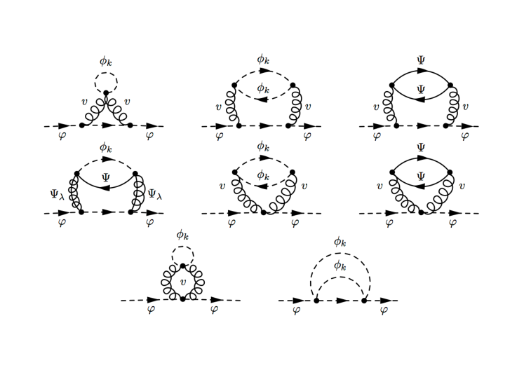
Figure 4.2: Virtual contributions to the self-energies of the scalar fields of the visible sector that lead to radiatively-induced masses. In the notation conventions of this figure, $\varphi$ stands for a generic scalar field of the visible sector, $v$ and $\Psi_{\lambda}$ for the gauge boson and gaugino field associated with the model gauge group, and $\phi_{k}$ and $\Psi$ for the scalar and four-component fermionic messenger fields, respectively.

Similarly, masses for the scalar fields of the visible sector can also be generated by quantum corrections, but this time at the two-loop level, as shown in Figure 4.2. The relevant loop diagrams involve, as for the gaugino case, standard gauge interactions depicted in the Lagrangian of Eq. (2.4.72) that apply both for the scalar fields of the visible sector and the messenger fields. Quantum corrections to the squared mass of a massless scalar field $\varphi$ of the visible sector are derived from the expression of the scalar propagator $-i\Pi$ evaluated on-shell

$$-i\Pi_{mn}(p)=-i\Pi(p)\delta_{mn}\qquad\Rightarrow\qquad\delta m^{2}_{\varphi}=\Pi(0)\ ,$$ (4.2.45)

where $m$ and $n$ are gauge indices related to the representation of the gauge group in which the field $\varphi$ lies. After an omitted (for brevity) computation, these two-loop quantum corrections are evaluated as

$$\boxed{\begin{split}\delta m^{2}_{\varphi}=&\ \frac{g^{4}}{128\pi^{4}}\tau_{\cal R}C_{\cal R}\bigg{[}\Big{(}M_{\rm mes}^{2}\!+\!\Lambda M_{\rm mes}\Big{)}\Big{(}\log\frac{M_{\rm mes}\!+\!\Lambda}{M_{\rm mes}}\!-\!2{\rm Li}_{2}\frac{\Lambda}{M_{\rm mes}\!+\!\Lambda}\!+\!\frac{1}{2}{\rm Li}_{2}\frac{2\Lambda}{M_{\rm mes}\!+\!\Lambda}\Big{)}\\ &\ +\Big{(}M_{\rm mes}^{2}\!-\!\Lambda M_{\rm mes}\Big{)}\Big{(}\log\frac{M_{\rm mes}\!-\!\Lambda}{M_{\rm mes}}\!-\!2{\rm Li}_{2}\frac{\Lambda}{\Lambda\!-\!M_{\rm mes}}\!+\!\frac{1}{2}{\rm Li}_{2}\frac{2\Lambda}{\Lambda\!-\!M_{\rm mes}}\Big{)}\bigg{]}\ ,\end{split}}$$ (4.2.46)

where $C_{\cal R}$ is the Casimir invariant associated to the representation ${\cal R}$,

$$\big{(}T^{a}T_{a}\big{)}^{m}{}_{n}=C_{\cal R}\ \delta^{m}{}_{n}\ .$$ (4.2.47)

The originally massless scalar fields have hence been rendered massive.

In gravity-mediated supersymmetry breaking, multiscalar soft interactions have been generated as illustrated in the Lagrangian of Eq. (4.2.23). The same kind of supersymmetry-breaking interactions are also induced by gauge-mediation. However, they arise, as for the scalar masses, at the two-loop level but can, in contrast to the mass terms, be approximately neglected at the messenger scale. The supersymmetry-breaking Lagrangian hence reads, collecting the terms related to the visible sector,

$$\boxed{\begin{split}{\cal L}_{\rm soft}=&\ -\frac{1}{2}m_{\lambda^{a}}\big{[}\lambda^{a}\!\cdot\!\lambda_{a}+{\bar{\lambda}}^{a}\!\cdot\!{\bar{\lambda}}_{a}\big{]}-m_{\varphi^{i}}^{2}\varphi^{\dagger}_{i}\varphi^{i}\ .\end{split}}$$ (4.2.48)

The gaugino and scalar masses $m_{\lambda^{a}}$ and $m_{\phi^{i}}$ are deduced from Eq. (4.2.43) and Eq. (4.2.46), respectively, and multiscalar interactions are only generated when evolving the soft supersymmetry-breaking parameters down to the electroweak scale.

4.2.4 Anomaly-mediated supersymmetry breaking

In this section, we present a mechanism where supersymmetry breaking is mediated to the visible sector through quantum loop effects related to anomalous rescaling violations [126, 127, 128]. This mechanism has the virtue to operate as soon as we have a hidden sector in the theory by means of several sources of anomalies and possibly competes with other sources of supersymmetry breaking. We take here the example of supergravity where supersymmetry breaking is also mediated by Weyl anomalies, although their contribution is strongly suppressed with respect to gravity effects.

In order to underline the effects of anomaly-mediated supersymmetry breaking, we start from the supergravity Lagrangian of Eq. (4.2.3) and replace the capacity ${\cal E}$ by the superfield product ${\cal E}\langle{\bf\Phi}\rangle^{3}$, introducing a spurious superfield ${\bf\Phi}$. The vacuum expectation value of the latter is explicitly given by

$$\big{\langle}{\bf\Phi}\big{\rangle}=1+M_{\rm aux}\ \theta\!\cdot\!\theta\ ,$$ (4.2.49)

so that $\langle{\bf\Phi}\rangle$ can be employed as a tool to select the lowest-order component of the supergravity multiplet included in the supervierbein,

$${\cal E}=e\big{\langle}{\bf\Phi}^{3}\big{\rangle}+\ldots$$ (4.2.50)

where higher spin states are contained in the dots. This computation artifact allows us to factorize out the pure gravity Lagrangian and only focus on the chiral and gauge content of the theory. The spurious superfield is hence used to rewrite the first term of the Lagrangian of Eq. (4.2.3) under an eight-dimensional integral upon the superspace coordinates. This uses a recasting of the kinetic and interaction terms included in the Kähler potential, neglecting gravitational contributions involving non-scalar states of the gravitation supermultiplet, where the relevant terms are made proportional to $\langle{\bf\Phi\Phi}^{\dagger}\rangle$ [188, 196]. Inserting the spurious superfield $\langle{\bf\Phi}\rangle$ into the other terms of the supergravity Lagrangian, the latter can be rewritten as

$$\begin{split}{\cal L}=&\ \frac{3e}{2\kappa^{2}}\int{\rm d}^{2}\Theta\ {\rm d}^{2}{\bar{\Theta}}\ \big{\langle}{\bf\Phi\Phi}^{\dagger}\big{\rangle}\ e^{-\frac{1}{3}\kappa^{2}K(\Phi,\Phi^{\dagger}e^{-2gV})}+e\int{\rm d}^{2}\Theta\ \big{\langle}{\bf\Phi}^{3}\big{\rangle}\ W(\Phi)\\ &\ +\frac{e}{16g^{2}}\int{\rm d}^{2}\Theta\ h_{ab}(\Phi)W^{a\alpha}W_{\alpha}^{b}+{\rm h.c.}+\ldots\ ,\end{split}$$ (4.2.51)

where the superfield $\Phi$ represents in a generic fashion the chiral content of the theory, $W_{\alpha}$ the superfield strength tensor associated with the gauge group and the dots stand for the omitted terms related to the gravity supermultiplet. We moreover assume that all the three fundamental functions, i.e., the Kähler potential $K$, the superpotential $W$ and the gauge kinetic function $h$, are independent of the spurious superfield ${\bf\Phi}$ and can be written as sums of two terms, one of them depending exclusively on the superfields of the visible sector and the other one being only related to the hidden sector where supersymmetry breaking occurs. The same Lagrangian could also have been obtained by employing the Weyl compensator formalism for the rescaling. In this case, it is sufficient to replace the compensator superfield appearing in the Lagrangian of Eq. (4.2.4) by its vacuum expectation value given by Eq. (4.2.49).

Inspecting the Lagrangian of Eq. (4.2.51), we observe that the super-Yang-Mills part of the Lagrangian (i.e., the term of the second line of this equation) does not couple to the spurious superfield $\langle{\bf\Phi}\rangle$. This is not surprising as the gauge sector is invariant under super-Weyl transformations. However, this symmetry is anomalous and broken via quantum loop effects [129, 130, 131, 132, 133]. Canceling this anomaly by appropriate counterterms balancing the effects of the relevant loop-diagrams yields a shift of the gauge kinetic function,

$$h_{ab}(\Phi)\to h_{ab}(\Phi)-2\ b_{0}\ \delta_{ab}\ \langle\log({\bf\Phi})\rangle\ ,$$ (4.2.52)

where $b_{0}$ stands for the one-loop coefficient of the gauge beta function $\beta_{g}$

$$\beta_{g}=-b_{0}g^{3}+\ldots\ .$$ (4.2.53)

After evaluating the integral upon $\Theta$ in the super-Yang-Mills Lagrangian, the shift of Eq. (4.2.52) generates a non-vanishing gaugino mass $m_{\lambda}$,

$$\boxed{m_{\lambda}=\frac{\beta_{g}}{g}M_{\rm aux}\ .}$$ (4.2.54)

This consists of a strong prediction of anomaly-mediated supersymmetry-breaking scenarios as this last equation means that the different gaugino masses appear as the ratio of the corresponding gauge beta functions when the gauge group is a semi-simple group.

As briefly mentioned above, there are other ways to generate anomalous mass terms for the gaugino fields, but they can all be considered as results of the violation of the super-Weyl invariance. We can associate a cutoff scale $\Lambda_{\rm UV}$ to these effects, related to a hidden sector embedding some mechanism for anomaly cancellation. In the case of supergravity, this scale is naturally the Planck scale. Renormalizable physics, i.e., physics related to the visible sector, is however independent of the nature of the cutoff. Therefore, the previous results of Eq. (4.2.54) can be safely generalized. To illustrate this statement, we introduce a renormalization scale $\mu_{R}$ and turn to the study of anomaly-induced supersymmetry-breaking terms in the general case.

After renormalization, the Wilsonian effective Lagrangian obtained after integrating out all the modes lying above $\Lambda_{\rm UV}$ (and thus included in the hidden sector) is given by

$$\begin{split}{\cal L}=&\ \int{\rm d}^{2}\theta\ {\rm d}^{2}{\bar{\theta}}\ Z^{i}{}_{j}\bigg{[}\frac{\mu_{R}}{\Lambda_{\rm UV}\langle{\bf\Phi}\rangle},\frac{\mu_{R}}{\Lambda_{\rm UV}\langle{\bf\Phi^{\dagger}}\rangle}\bigg{]}\Phi_{i}^{\dagger}e^{-2gV}\Phi^{j}+\int{\rm d}^{2}\theta\ W(\Phi)\\ &\ +\frac{1}{16g^{2}}\int{\rm d}^{2}\theta\ \tau_{ab}\bigg{[}\frac{\mu_{R}}{\Lambda_{\rm UV}\langle{\bf\Phi}\rangle}\bigg{]}W^{a\alpha}W_{\alpha}^{b}+{\rm h.c.}\ .\end{split}$$ (4.2.55)

This last expression can be computed by starting from Eq. (4.2.51), then performing a Taylor expansion of the exponential and finally evaluating the results in the flat space limit,

$$\Theta\to\theta\ ,\qquad{\bar{\Theta}}\to{\bar{\theta}}\qquad\text{and}\qquad e\to 1\ .$$ (4.2.56)

The tree-level dependence in the spurious superfield is shifted away by the superfield redefinitions

$$\Phi\langle{\bf\Phi}\rangle\to\Phi\ ,$$ (4.2.57)

so that the dependence in $\langle{\bf\Phi}\rangle$ now only occurs through loop-effects embedded into the functions $Z$ and $\tau$. In other words, there is no tree-level communication of supersymmetry breaking. In order to write such a form for the Lagrangian, we have assumed that the superpotential is trilinear and homogeneous in the chiral superfields of the visible sector, as it originally multiplies a third power of the spurious superfield and there is no more dependence on $\langle{\bf\Phi}\rangle$ in the superpotential Lagrangian of Eq. (4.2.55). The generation of superpotential mass and linear terms is however still possible dynamically, once supersymmetry is broken [126, 197, 198, 199]. Moreover, the absence of renormalization effects in the superpotential term of Eq. (4.2.55) is justified by the supersymmetric non-renormalization theorems [28, 24, 96, 200, 201, 202, 203]. To summarize, the spurious superfield, and in particular its vacuum expectation value $\langle{\bf\Phi}\rangle$, are the only quantities encompassing the effects of the hidden sector which left in the effective Lagrangian.

The form of the functions $Z$ and $\tau$, as well as the one of their arguments can be obtained by means of the classical $R$-symmetry of the Lagrangian. Before the rescaling of Eq. (4.2.57), the tree-level Lagrangian is manifestly $R$-symmetric after assigning a vanishing $R$-charge to the chiral superfields $\Phi$ and a $R$-charge of 2/3 for the spurious superfield, since the superpotential has been chosen as a trilinear and homogeneous function of the chiral superfields. At the one-loop level, the situation is however highly different. Firstly, counterterms that depend on a cutoff scale $\Lambda_{\rm UV}$ must be added to the theory so that the one-loop ultraviolet divergences are compensated. Secondly, the rescaling of the matter fields does not allow to fully eliminate the dependence in $\langle{\bf\Phi}\rangle$ issued from the loop diagrams but only the tree-level one. It has been found that the latter always appears through a product with the cutoff scale [126, 133, 204], so that the holomorphic function $\tau$ only depends on the product $\Lambda_{\rm UV}\langle{\bf\Phi}\rangle$, while the function $Z$ depends in addition on the conjugate quantity $\Lambda_{\rm UV}\langle{\bf\Phi}^{\dagger}\rangle$. After the rescaling, all chiral superfields $\Phi$ get a $R$-charge of 2/3, as shown by Eq. (4.2.57). Since the $R$-symmetry is (formally) exact, the function $Z$ is enforced to depend on the spurious superfield only through a $R$-invariant products of ${\bf\Phi}$ and ${\bf\Phi}^{\dagger}$,

$$Z^{i}{}_{j}\bigg{[}\frac{\mu_{R}}{\Lambda_{\rm UV}\langle{\bf\Phi}\rangle},\frac{\mu_{R}}{\Lambda_{\rm UV}\langle{\bf\Phi^{\dagger}}\rangle}\bigg{]}\to Z^{i}{}_{j}\bigg{[}\frac{\mu_{R}}{\Lambda_{\rm UV}\langle|{\bf\Phi}|\rangle}\bigg{]}\ .$$ (4.2.58)

Turning off the effects of the hidden sector, i.e., fixing $\langle{\bf\Phi}\rangle$ to unity, the $R$-symmetry becomes explicitly broken in the gauge sector, a consequence of the well-known anomalies of the $R$-symmetry. Curing these anomalies by means of appropriate counterterms therefore implies a shift of the function $\tau$ that restores the $R$-symmetry. The anomalies impose in this way the form of the function $\tau$, which is found to be similar to Eq. (4.2.52),

$$\tau_{ab}\bigg{[}\frac{\mu_{R}}{\Lambda_{\rm UV}\langle{\bf\Phi}\rangle}\bigg{]}=h_{ab}+2b_{0}\delta_{ab}\log\frac{\mu_{R}}{\Lambda_{\rm UV}\langle{\bf\Phi}\rangle}\ .$$ (4.2.59)

This shows that gaugino mass term at a scale $\mu_{R}$ are obtained according to renormalization group running from the cutoff scale $\Lambda_{\rm UV}\langle{\bf\Phi}\rangle$ to $\mu_{R}$, the results of Eq. (4.2.52) being retrieved after Taylor-expanding the logarithm of the spurion superfield.

We have so far proved that super-Weyl anomalies are responsible for generating gaugino mass terms. Other soft supersymmetry-breaking terms can also be generated by anomalies. To underline such effects, one proceeds with the computation of the Taylor expansion of the wave function $Z$ associated with the chiral superfield $\Phi$ with respect to $M_{\rm aux}$. Understanding superfield indices, one finds

$$\begin{split}\log Z\bigg{[}\frac{\mu_{R}}{\Lambda_{\rm UV}\langle|{\bf\Phi}|\rangle}\bigg{]}=&\ \log\frac{\mu_{R}}{\Lambda_{\rm UV}}-\frac{1}{2}\gamma(g,y)M_{\rm aux}\ \theta\!\cdot\!\theta-\frac{1}{2}\gamma(g,y)M_{\rm aux}^{\ast}\ {\bar{\theta}}\!\cdot\!{\bar{\theta}}\\ &\ +\frac{1}{4}\big{|}M_{\rm aux}\big{|}^{2}\Big{[}\frac{\partial\gamma(g,y)}{\partial\beta}\beta_{g}+\frac{\partial\gamma(g,y)}{\partial y}\beta_{y}\Big{]}\ \theta\!\cdot\!\theta\ {\bar{\theta}}\!\cdot\!{\bar{\theta}}\ ,\end{split}$$ (4.2.60)

where we have introduced the anomalous dimension of the superfield $\Phi$,

$$\gamma(g,y)=\frac{\partial\log Z}{\partial\log\mu_{R}}\ ,$$ (4.2.61)

and the beta functions

$$\beta_{g}=\frac{\partial g}{\partial\log\mu_{R}}\qquad\text{and}\qquad\beta_{y}=\frac{\partial y}{\partial\log\mu_{R}}\ .$$ (4.2.62)

In our notations, the quantity $y$ generically denotes any superpotential coupling and $g$ stands for the gauge coupling constant. As far as mass terms are concerned, the lower-order coefficients of the Grassmann expansion of $\log Z$ can be rescaled away,

$$\exp\bigg{[}\frac{1}{2}\log\frac{\mu_{R}}{\Lambda_{\rm UV}}-\frac{1}{2}\gamma(g,y)M_{\rm aux}\ \theta\!\cdot\!\theta\bigg{]}\langle{\bf\Phi}\rangle\to\langle{\bf\Phi}\rangle\ ,$$ (4.2.63)

so that after integration upon the Grassmann variables, the first term of the Lagrangian of Eq. (4.2.55) contains a scalar mass term, the related mass parameter $m_{\phi}^{2}$ evaluated at the renormalization scale $\mu_{R}$ reading

$$\boxed{m_{\phi}^{2}(\mu_{R})=-\frac{1}{4}\big{|}M_{\rm aux}\big{|}^{2}\bigg{[}\frac{\partial\gamma}{\partial\beta}\beta_{g}+\frac{\partial\gamma}{\partial y}\beta_{y}\bigg{]}\ .}$$ (4.2.64)

Scalar masses hence arise at the two-loop level, in contrast to the gaugino masses which are induced by one-loop effects shown in Eq. (4.2.54), since the leading contributions to the scalar masses are derived from the knowledge of coefficients of the anomalous dimension and the beta functions already computed at the one-loop order. Schematically, they can be written as

$$\gamma(g,y)=\gamma_{g}g^{2}+\gamma_{y}y^{2}\ ,\qquad\beta_{g}=-b_{0}g^{3}\qquad\text{and}\qquad\beta_{y}=y\big{(}y_{y}y^{2}+y_{g}g^{2}\big{)}\ ,$$ (4.2.65)

where $\gamma_{g}$ is always positive and real while the other parameters could be positive or negative real numbers. In particular, $\gamma_{y}$ is negative for infrared-free gauge theories, so that some scalar masses can become tachyonic if no other source of supersymmetry breaking allows for balancing the negative effects.

The shift of Eq. (4.2.63) also induces effects in the superpotential Lagrangian, i.e., in the second term of Eq. (4.2.55). Recalling that the superpotential only consists of trilinear interaction terms, this shift leads to supersymmetry-breaking trilinear scalar interactions. Denoting generically by $y_{ijk}$ a superpotential interaction that couples the superfields $\Phi^{i}$, $\Phi^{j}$ and $\Phi^{k}$, the associated soft supersymmetry-breaking coupling strength $A_{ijk}$ is hence given by

$$\boxed{A_{ijk}=\frac{1}{2}y_{ijk}\Big{[}\gamma_{i}+\gamma_{j}+\gamma_{k}\Big{]}M_{\rm aux}\ ,}$$ (4.2.66)

where $\gamma_{i}$, $\gamma_{j}$ and $\gamma_{k}$ are the anomalous dimensions related to the superfields $\Phi^{i}$, $\Phi^{j}$ and $\Phi^{k}$, respectively.

Collecting all the results derived above, the soft supersymmetry-breaking Lagrangian induced by anomalies can be written as

$$\boxed{\begin{split}{\cal L}_{\rm soft}=&\ -\frac{1}{2}m_{\lambda}\big{[}\lambda^{a}\!\cdot\!\lambda_{a}+{\bar{\lambda}}^{a}\!\cdot\!{\bar{\lambda}}_{a}\big{]}-m_{\phi^{i}}^{2}\ \phi^{\dagger}_{i}\phi^{i}-\Big{[}\frac{1}{6}A_{ijk}\phi^{i}\phi^{j}\phi^{k}+{\rm h.c.}\Big{]}\ ,\end{split}}$$ (4.2.67)

where the gaugino masses are given by Eq. (4.2.54), the scalar masses by Eq. (4.2.64) and the trilinear couplings by Eq. (4.2.66). In addition, the form of these soft terms is renormalization-group invariant and therefore holds at any scale. This consequently entails large predictivity for anomaly-mediated supersymmetry-breaking scenarios, with fixed mass ratios and distinctive signatures [205, 206, 207, 208, 209].

4.3 Renormalization group equations for supersymmetry

In the three supersymmetry-breaking scenarios introduced in Section 4.2.2, Section 4.2.3 and Section 4.2.4, supersymmetry breaking occurs at a high energy-scale. In order to investigate the related phenomenology, but at the electroweak scale, the generated soft terms must be subsequently run down. Assuming a renormalizable (softly-broken) supersymmetric theory and only focusing on the visible sector, the supersymmetric pieces of the action are given as in Eq. (2.4.70),

$$\begin{split}{\cal S}=&\ \int{\rm d}^{4}x\ {\rm d}^{2}\theta\ {\rm d}^{2}{\bar{\theta}}\ \Phi^{\dagger}e^{-2gV}\Phi+\int{\rm d}^{4}x\ {\rm d}^{2}\theta\ W(\Phi)+\int{\rm d}^{4}x\ {\rm d}^{2}{\bar{\theta}}\ W^{\star}(\Phi^{\dagger})\\ &\ +\frac{1}{16g^{2}}\int{\rm d}^{4}x\ {\rm d}^{2}\theta\ W^{a\alpha}W_{a\alpha}+\frac{1}{16g^{2}}\int{\rm d}^{4}x\ {\rm d}^{2}{\bar{\theta}}\ {\overline{W}}^{a}_{\dot{\alpha}}{\overline{W}}_{a}^{\dot{\alpha}}\ ,\end{split}$$ (4.3.1)

where we have chosen the gauge kinetic function and the Kähler potential in a minimal way, as given by Eq. (2.4.68). We recall that in our conventions, the Lagrangian above describes the dynamics of a set of matter supermultiplets that are represented by chiral superfields $\Phi$. These superfields lie in given representations of a gauge group $G$ with which we associate the coupling constant $g$ and the vector superfield $V$. Finally, kinetic and gauge interaction terms for the components of the superfield $V$ are derived from the sum of the squares of the superfield strength tensors $W_{\alpha}$ and ${\overline{W}}_{\dot{\alpha}}$, as usual.

For a renormalizable theory, the superpotential $W$ is a gauge-invariant function at most trilinear in the chiral content of the theory, as given in Eq. (2.4.69),

$$W(\Phi)=\frac{1}{6}\lambda_{ijk}\Phi^{i}\Phi^{j}\Phi^{k}+\frac{1}{2}\mu_{ij}\Phi^{i}\Phi^{j}+\xi_{i}\Phi^{i}\ ,$$ (4.3.2)

where $\lambda$, $\mu$ and $\xi$ are free parameters of the model.

In addition to the supersymmetric Lagrangian, one also needs to consider supersymmetry-breaking soft terms generically written as

$${\cal L}_{\rm soft}=-\frac{1}{6}a_{ijk}\phi^{i}\phi^{j}\phi^{k}-\frac{1}{2}b_{ij}\phi^{i}\phi^{j}-c_{i}\phi^{i}-\frac{1}{2}M\lambda\!\cdot\!\lambda-\frac{1}{2}\phi^{\dagger}_{i}(m^{2})^{i}{}_{j}\phi^{j}+{\rm h.c.},$$ (4.3.3)

where the parameters $a$, $b$, $c$ denote the interaction strengths of the supersymmetry-breaking multiscalar interactions, $M$ the gaugino masses and $m^{2}$ the squared mass matrix associated with the scalar fields of the theory. In the Lagrangian above, the scalar components of the matter supermultiplets are denoted by $\phi$ while the gaugino component of the vector supermultiplet $V$ is represented by $\lambda$.

These parameters are related to the supersymmetry-breaking mechanism and are in principle known at the (high) scale where supersymmetry breaking occurs. The derivation of the values of those parameters at the electroweak scale, relevant for, e.g., collider phenomenology, is driven by supersymmetric renormalization group equations. These equations link the low-energy parameters to their high-energy counterparts. Although the number of free parameters can be quite large, some organizing principles in general hold at the supersymmetry-breaking scale so that we end up with a few input parameters at the high scale.

The supersymmetric renormalization group equations have been known at the one-loop level [210, 211] and two-loop level for a long time [212, 213, 214, 215, 216] and are generically written as

$$\frac{{\rm d}}{{\rm d}t}x=\beta_{x}\qquad\text{with}\qquad\beta_{x}=\frac{1}{16\pi^{2}}\beta_{x}^{(1)}+\frac{1}{(16\pi^{2})^{2}}\beta_{x}^{(2)}+\ldots\ ,$$ (4.3.4)

where $x$ stands for any parameter and $\beta_{x}$ for the associated beta function. This function is thus calculated perturbatively, $\beta_{x}^{(1)}$ and $\beta_{x}^{(2)}$ being the one-loop and two-loop coefficients, respectively.

Starting with the gauge sector, the first coefficients of the $\beta$-functions of the gauge coupling constant $g$ and of the gaugino mass parameter $M$ read

$$\beta_{g}^{(1)}=g^{3}\Big{[}\tau-3C_{G}\Big{]}\qquad\text{and}\qquad\beta_{M}^{(1)}=2g^{2}M\Big{[}\tau-3C_{G}\Big{]}\ ,$$ (4.3.5)

whilst the two-loop coefficients are given, in the $\overline{DR}$ renormalization scheme, by

$$\begin{split}\beta_{g}^{(2)}=&\ g^{5}\Big{[}-6C_{G}^{2}+2C_{G}\tau+4\tau_{\cal R}C_{\cal R}\Big{]}-g^{3}\lambda^{\ast ijk}\lambda_{ijk}C_{k}/d_{G}\ ,\\ \beta_{M}^{(2)}=&\ 4g^{4}M\Big{[}-6C_{G}^{2}+2C_{G}\tau+4\tau_{\cal R}C_{\cal R}\Big{]}+2g^{2}\lambda_{ijk}\Big{[}a^{\ast ijk}-M\lambda^{\ast ijk}\Big{]}C_{k}/d_{G}\ .\end{split}$$ (4.3.6)

Considering a chiral superfield lying in a representation ${\cal R}$ of the gauge group, we denote by $C_{\cal R}$ the quadratic Casimir invariant associated with this representation. Similarly, $C_{G}$ is the quadratic Casimir invariant relative to the adjoint representation and $C_{k}$ corresponds to the Casimir invariant associated with the representation in which the chiral superfield $\Phi^{k}$ lies. In addition, we have also introduced $\tau$ as the total Dynkin index of the gauge group, i.e., the Dynkin index summed over all the chiral content of the model, accounting for the superfield multiplicity. Moreover, the quantity $C_{\cal R}\tau_{\cal R}$ contains an implicit summation. It refers to a sum of the Dynkin indices over all the chiral superfields of the model, weighted by the corresponding quadratic Casimir invariants. Finally, the dimension of the gauge group is denoted by $d_{G}$.

On the basis of the supersymmetric non-renormalization theorems [24, 28, 96, 200, 201, 202, 203], the evolution of the superpotential parameters is entirely driven by the anomalous dimensions of the fields (see Section 4.2.4). The first and second coefficients of the $\beta$-functions of the linear, bilinear and trilinear interaction parameters $\xi$, $\mu$ and $\lambda$ are then given by

$$\begin{split}\beta_{\xi_{i}}^{(n)}=&\ \xi_{p}\ (\gamma^{(n)})^{p}{}_{i}\ ,\\ \beta_{\mu_{ij}}^{(n)}=&\ \mu_{ip}\ (\gamma^{(n)})^{p}{}_{j}+\mu_{pj}\ (\gamma^{(n)})^{p}{}_{i}\ ,\\ \beta_{\lambda_{ijk}}^{(n)}=&\ \lambda_{ijp}\ (\gamma^{(n)})^{p}{}_{k}+\lambda_{ipk}\ (\gamma^{(n)})^{p}{}_{j}+\lambda_{pjk}\ (\gamma^{(n)})^{p}{}_{i}\ ,\end{split}$$ (4.3.7)

respectively, with $n=1$ or 2. The first two coefficients of the anomalous dimensions $\gamma$ appearing in these beta functions are given by

$$\begin{split}(\gamma^{(1)})^{j}{}_{i}=&\ \frac{1}{2}\lambda_{ipq}\lambda^{\ast jpq}-2\delta^{j}{}_{i}g^{2}C_{i}\ ,\\ (\gamma^{(2)})^{j}{}_{i}=&\ g^{2}\lambda_{ipq}\lambda^{\ast jpq}\Big{[}2C_{p}\!-\!C_{i}\Big{]}\!-\!\frac{1}{2}\lambda_{imn}\lambda^{\ast npq}\lambda_{pqr}\lambda^{\ast mrj}\!+\!2\delta^{j}{}_{i}g^{4}C_{i}\Big{[}\tau\!+\!2C_{i}\!-\!3C_{G}\Big{]}\ .\end{split}$$ (4.3.8)

We now turn to the evolution of the supersymmetry-breaking parameters. The first coefficients of the beta functions related to the linear, bilinear and trilinear scalar interactions read

$$\begin{split}\beta_{c_{i}}^{(1)}=&\ \frac{1}{2}\lambda_{ipq}\lambda^{\ast rpq}c_{r}\!+\!\lambda^{\ast rpq}a_{ipq}\xi_{r}\!+\!\mu_{ir}\lambda^{\ast rpq}b_{pq}\!+\!2\lambda_{ipq}(m^{2})^{q}{}_{r}\mu^{\ast pr}\!+\!a_{ipq}b^{\ast pq}\ ,\\ \beta_{b_{ij}}^{(1)}=&\ \frac{1}{2}b_{ip}\lambda^{\ast pqr}\lambda_{qrj}\!+\!\frac{1}{2}\lambda_{ijr}\lambda^{\ast rpq}b_{pq}\!+\!\mu_{ip}\lambda^{\ast pqr}a_{qrj}\!-\!2g^{2}C_{i}\big{[}b_{ij}\!-\!2M\mu_{ij}\big{]}\\ &\ +\frac{1}{2}b_{jp}\lambda^{\ast pqr}\lambda_{qri}\!+\!\frac{1}{2}\lambda_{jir}\lambda^{\ast rpq}b_{pq}\!+\!\mu_{jp}\lambda^{\ast pqr}a_{qri}\!-\!2g^{2}C_{j}\big{[}b_{ji}\!-\!2M\mu_{ji}\big{]}\ ,\\ \beta_{a_{ijk}}^{(1)}=&\ \frac{1}{2}a_{ijr}\lambda^{\ast rpq}\lambda_{pqk}\!+\!\lambda_{ijr}\lambda^{\ast rpq}a_{pqk}\!-\!2g^{2}C_{k}\big{[}a_{ijk}\!-\!2M\lambda_{ijk}\big{]}\\ &\ +\frac{1}{2}a_{kjr}\lambda^{\ast rpq}\lambda_{pqi}\!+\!\lambda_{kjr}\lambda^{\ast rpq}a_{pqi}\!-\!2g^{2}C_{i}\big{[}a_{kji}\!-\!2M\lambda_{kji}\big{]}\\ &\ +\frac{1}{2}a_{ikr}\lambda^{\ast rpq}\lambda_{pqj}\!+\!\lambda_{ikr}\lambda^{\ast rpq}a_{pqj}\!-\!2g^{2}C_{j}\big{[}a_{ikj}\!-\!2M\lambda_{ikj}\big{]}\ ,\end{split}$$ (4.3.9)

while the second coefficients of these beta functions are given by

$$\begin{split}\beta_{c_{i}}^{(2)}=&\ 4g^{2}C_{q}\Big{[}\big{(}a_{ipq}\!-\!\lambda_{ipq}M\big{)}\big{(}\lambda^{\ast rpq}\xi_{r}\!+\!b^{\ast pq}\big{)}\!+\!\frac{1}{2}\lambda_{ipq}\lambda^{\ast rpq}c_{r}\!-\!\lambda^{\ast rpq}\big{(}\mu_{pq}M\!-\!b_{pq}\big{)}\mu_{ir}\\ &\ +\big{(}\lambda_{ipq}(m^{2})^{p}{}_{r}\!+\!\lambda_{irp}(m^{2})^{p}{}_{q}\!+\!2\lambda_{irq}|M|^{2}\!-\!a_{irq}M^{*}\big{)}\mu^{\ast rq}\Big{]}\\ &\ -\Big{[}\lambda_{ipq}a_{trs}+a_{ipq}\lambda_{trs}\Big{]}\lambda^{\ast qrs}\lambda^{\ast kpt}\xi_{k}-\frac{1}{2}\lambda_{ipq}\lambda^{\ast qrs}\lambda_{trs}\lambda^{\ast kpt}c_{k}\\ &\ -\Big{[}a_{qst}\mu_{pk}+\lambda_{qst}b_{pk}\Big{]}\lambda^{\ast kst}\lambda^{\ast rpq}\mu_{ir}-\Big{[}\lambda_{ipq}a_{rst}+a_{ipq}\lambda_{rst}\Big{]}\lambda^{\ast qst}b^{\ast pr}\\ &\ -\!\Big{[}\big{(}\lambda_{ikq}(m^{2})^{k}{}_{p}\lambda_{rst}\!+\!\lambda_{ipq}(m^{2})^{k}{}_{r}\lambda_{kst}\!+\!2\lambda_{ipq}(m^{2})^{t}{}_{k}\lambda_{rst}\!+\!\lambda_{ipk}(m^{2})^{k}{}_{q}\lambda_{rst}\big{)}\lambda^{\ast qst}\\ &\ +\!\big{(}\lambda_{ipq}a_{rst}-a_{ipq}\lambda_{rst}\big{)}a^{\ast qst}\Big{]}\mu^{\ast pr}\ ,\\ \beta_{b_{ij}}^{(2)}=&\ g^{2}\lambda^{\ast rpq}\Big{\{}2C_{p}\lambda_{ijr}\big{(}b_{pq}\!-\!\mu_{pq}M\big{)}\!+\!\big{(}2C_{p}\!-\!C_{i}\big{)}\Big{[}b_{ir}\lambda_{pqj}\!+\!2\mu_{ir}\big{(}a_{pqj}\!-\!\lambda_{pqj}M\big{)}\Big{]}\Big{\}}\\ &\ +2g^{4}\big{(}b_{ij}\!-\!4\mu_{ij}M\big{)}\big{(}C_{i}\tau\!+\!2C_{i}^{2}\!-\!3C_{G}C_{i}\big{)}\!-\!\frac{1}{2}\Big{[}b_{ip}\lambda_{qkj}\!+\!b_{qk}\lambda_{ijp}\Big{]}\lambda_{str}\lambda^{\ast pqr}\lambda^{\ast stk}\\ &\ -\!\Big{[}\frac{1}{2}\lambda_{ijs}\mu_{tr}a_{pqk}\!+\!\mu_{is}\big{(}a_{kpq}\lambda_{trj}\!+\!\lambda_{kpq}a_{trj}\big{)}\Big{]}\lambda^{\ast pqr}\lambda^{\ast stk}+(i\leftrightarrow j)\ ,\\ \beta_{a_{ijk}}^{(2)}=&\ -\lambda^{\ast smn}\lambda^{\ast pqr}\Big{[}\frac{1}{2}a_{ijs}\lambda_{npq}\lambda_{mrk}+\lambda_{ijs}\big{(}\lambda_{npq}a_{mrk}+a_{npq}\lambda_{mrk}\big{)}\Big{]}\\ &\ +g^{2}\big{(}2C_{p}-C_{k}\big{)}\lambda^{\ast rpq}\Big{[}a_{ijr}\lambda_{pqk}+2\lambda_{ijr}\big{(}a_{pqk}-M\lambda_{pqk}\big{)}\Big{]}\\ &\ +2g^{4}\big{(}a_{ijk}-4M\lambda_{ijk}\big{)}\big{(}C_{k}\tau+2C_{k}^{2}-3C_{G}C_{k}\big{)}+(k\leftrightarrow i)+(k\leftrightarrow j)\ .\end{split}$$ (4.3.10)

Finally, we achieve this section by providing the first two coefficients of the beta function associated to the scalar mass parameters,

$$\begin{split}\beta^{(1)}_{(m^{2})^{i}{}_{j}}=&\ \frac{1}{2}\lambda^{\ast ipq}\lambda_{pqr}(m^{2})^{r}{}_{j}+\frac{1}{2}\lambda_{jpq}\lambda^{\ast pqr}(m^{2})^{i}{}_{r}+2\lambda^{\ast ipq}\lambda_{jpr}(m^{2})^{r}{}_{q}+a_{jpq}a^{\ast ipq}\\ &\ -8\delta^{i}{}_{j}MM^{\dagger}g^{2}C_{i}+2g^{2}(T_{a})^{i}{}_{j}{\rm Tr}\big{[}T^{a}m^{2}\big{]}\ ,\end{split}$$ (4.3.11)

and

$$\begin{split}\beta^{(2)}_{(m^{2})^{i}{}_{j}}=&\ \delta^{i}{}_{j}g^{4}\bigg{[}MM^{\dagger}\Big{(}24\tau C_{i}\!+\!48C_{i}^{2}\!-\!72C_{G}C_{i}\Big{)}+8C_{i}\Big{(}{\rm Tr}\big{[}\tau_{\cal R}m^{2}\big{]}\!-\!C_{G}MM^{\dagger}\Big{)}\bigg{]}\\ &\ -2g^{2}(T_{a})^{i}{}_{j}\big{(}T^{a}m^{2}\big{)}^{r}{}_{s}\lambda^{\ast spq}\lambda_{rpq}+8g^{4}(T_{a})^{i}{}_{j}{\rm Tr}\big{[}T^{a}C_{\cal R}m^{2}\big{]}\\ &\ +g^{2}\big{(}C_{p}\!+\!C_{q}\!-\!C_{i}\big{)}\Big{[}(m^{2})^{i}{}_{s}\lambda^{\ast spq}\lambda_{jpq}\!+\!\lambda^{\ast ipq}\lambda_{spq}(m^{2})^{s}{}_{j}\!+\!4\lambda^{\ast ipq}\lambda_{jps}(m^{2})^{s}{}_{q}\\ &\ +2a^{\ast ipq}\big{(}a_{jpq}-\lambda_{jpq}M\big{)}-2\lambda^{\ast ipq}\big{(}a_{jpq}M^{\dagger}-2\lambda_{jpq}MM^{\dagger}\big{)}\Big{]}\\ &\ -\lambda^{\ast ism}\bigg{[}\lambda_{jnm}\Big{(}(m^{2})^{r}{}_{s}\lambda^{\ast npq}\lambda_{rpq}\!+\!(m^{2})^{n}{}_{r}\lambda^{\ast rpq}\lambda_{spq}\Big{)}\!+\!\lambda_{jnr}(m^{2})^{n}{}_{s}\lambda^{\ast pqr}\lambda_{pqm}\\ &\ +2\lambda_{jsn}(m^{2})^{r}{}_{q}\lambda^{\ast npq}\lambda_{mpr}\bigg{]}\!-\!\Big{[}a^{\ast ism}\lambda^{\ast npq}\!+\!\lambda_{jsn}a_{mpq}\Big{]}\Big{[}a_{jsn}\lambda_{mpq}\!+\!\lambda_{jsn}a_{mpq}\Big{]}\\ &\ -\frac{1}{2}\lambda_{pqn}\lambda^{\ast pqr}\Big{[}(m^{2})^{i}{}_{s}\lambda^{\ast smn}\lambda_{mrj}+(m^{2})^{s}{}_{j}\lambda_{smr}\lambda^{\ast mni}\Big{]}\ .\end{split}$$ (4.3.12)

The terms depending explicitly on the representation matrices of the gauge group vanish identically for non-abelian groups. We recall that in the abelian case, these matrices must be read as squared abelian charges. Moreover, the Casimir invariant $C_{\cal R}$ and Dynkin index $\tau_{\cal R}$ appearing in some of these terms is associated with the representation of the relevant fields in the traces.

Chapter 5 The Minimal Supersymmetric Standard Model

In Chapter 2 and Chapter 4, we have shown how to construct any softly-broken supersymmetric field theory from very basic principles. In this chapter, we apply all the concepts that have been introduced so far in order to build the simplest phenomenologically relevant supersymmetric model, namely the Minimal Supersymmetric Standard Model or MSSM. We start with a detailed description of the construction of the model itself in Section 5.1, including details on the most popular choices for breaking supersymmetry in that framework and then detail the main features of the model in Section 5.2. One of the drawbacks of the MSSM, similarly to large classes of beyond the Standard Model theories, consists of its very large parameter space and the subsequent difficulties in designing non-experimentally excluded benchmark scenarios which implies to account for strong constraints from many experimental data. In this prospect, we study in Section 5.3 several low-energy electroweak and flavor observables in the context of the MSSM and dedicate Section 5.4 to the investigation of its cosmological aspects. We next address the more recent direct constraints extracted from the Large Hadron Collider data in Section 5.5, including the observation of a 125 GeV state compatible with the Standard Model Higgs boson [11, 12] and finally shortly motivate the needs to go beyond the MSSM in Section 5.6.

5.1 Construction of the model

5.1.1 Field content

The Minimal Supersymmetric Standard Model is the simplest supersymmetric model extending the Standard Model of particle physics [31, 32]. It results from the straightforward supersymmetrization of the Standard Model with the same gauge interactions, based on the semi-simple gauge group $SU(3)_{c}\times SU(2)_{L}\times U(1)_{Y}$. Because of their quantum numbers, the Standard Model particles cannot be gathered into $N=1$ representations of the Poincaré superalgebra (see Section 2.2.3). It is consequently necessary to embed each of the Standard Model degrees of freedom within a chiral or vector supermultiplet, supplementing it with one new state.

Supermultiplet	Standard Model fermion	Superpartner	Representation
$Q_{L}^{i}$
	$q_{L}^{i}=\begin{pmatrix}u_{L}^{i}\\ d_{L}^{i}\end{pmatrix}$	$\tilde{q}^{i}_{L}=\begin{pmatrix}\tilde{u}^{i}_{L}\\ \tilde{d}^{i}_{L}\end{pmatrix}$	$({\utilde{\bf 3}},{\utilde{\bf 2}},\frac{1}{6})$
$U^{i}_{R}$	$u_{R}^{ic}$	$\tilde{u}_{R}^{i{\dagger}}$	$({\utilde{\bf\bar{3}}},{\utilde{\bf 1}},-\frac{2}{3})$
$D_{R}^{i}$	$d_{R}^{ic}$	$\tilde{d}_{R}^{i{\dagger}}$	$({\utilde{\bf\bar{3}}},{\utilde{\bf 1}},\frac{1}{3})$
$L_{L}^{i}$
	$\ell_{L}^{i}=\begin{pmatrix}\nu_{L}^{i}\\ e_{L}^{i}\end{pmatrix}$	$\tilde{\ell}_{L}^{i}=\begin{pmatrix}\tilde{\nu}^{i}_{L}\\ \tilde{e}^{i}_{L}\end{pmatrix}$	$({\utilde{\bf 1}},{\utilde{\bf 2}},-\frac{1}{2})$
$E_{R}^{i}$	$e_{R}^{ic}$	$\tilde{e}_{R}^{i{\dagger}}$	$({\utilde{\bf 1}},{\utilde{\bf 1}},1)$
$N_{R}^{i}$	$\nu_{R}^{ic}$	$\tilde{\nu}_{R}^{i{\dagger}}$	$({\utilde{\bf 1}},{\utilde{\bf 1}},0)$

Table 5.1: The MSSM matter sector resulting from the supersymmetrization of the Standard Model quark and lepton fields. The representations under $SU(3)_{c}\times SU(2)_{L}\times U(1)_{Y}$ are provided in the last column of the table and the superscript $c$ denotes charge conjugation.

The matter sector of the theory consists of three generations of six chiral supermultiplets containing the Standard Model quarks and leptons, together with their squark and slepton superpartners. The corresponding superfields and their representations under the MSSM gauge group read

$$\begin{split}&\ Q_{L}^{i}=({\utilde{\bf 3}},{\utilde{\bf 2}},\phantom{-}\frac{1}{6})\quad,\quad U_{R}^{i}=({\utilde{\bf\bar{3}}},{\utilde{\bf 1}},-\frac{2}{3})\quad,\quad D_{R}^{i}=({\utilde{\bf\bar{3}}},{\utilde{\bf 1}},\frac{1}{3})\quad,\quad\\ &\ L_{L}^{i}=({\utilde{\bf 1}},{\utilde{\bf 2}},-\frac{1}{2})\quad,\quad E_{R}^{i}=({\utilde{\bf 1}},{\utilde{\bf 1}},\phantom{-}1)\quad,\quad N_{R}^{i}=({\utilde{\bf 1}},{\utilde{\bf 1}},0)\quad,\end{split}$$ (5.1.1)

where $i=1,2,3$ stands for a generation index and where the right-handed neutrino superfields $N_{R}$ are included for completeness. In our notations, we have employed the hypercharge quantum numbers as ‘representations’ for the $U(1)_{Y}$ subgroup. The physical component fields embedded into these superfields are detailed in Table 5.1. Usually, four-component spinorial representations of the Poincaré algebra are employed to describe (massive) quarks and leptons. Denoting such a four-component spinor $\Psi$ by

$$\Psi=\begin{pmatrix}\chi_{\alpha}\\ {\bar{\xi}}^{\dot{\alpha}}\end{pmatrix}\ ,$$ (5.1.2)

allows us to put an emphasis on its two-component fermionic content. This field combines a left-handed Weyl fermion $\chi$ and a right-handed Weyl fermion ${\bar{\xi}}$. However, only left-handed Weyl fermions can be employed to construct supersymmetric theories. This issue is cured by means of the charge conjugate Dirac field $\Psi^{c}$,

$$\Psi^{c}=C{\bar{\Psi}}^{t}=\begin{pmatrix}\xi_{\alpha}\\ {\bar{\chi}}^{\dot{\alpha}}\end{pmatrix}\ ,$$ (5.1.3)

where $C$ is the charge-conjugation operator. To supersymmetrize a non-supersymmetric theory with Dirac fermions by employing left-handed chiral superfields, the left-handed components of both the Dirac fields and their charge-conjugate counterparts are hence employed. In the example of the MSSM, it means that the superfields lying in the fundamental representation $\utilde{\bf 2}$ of $SU(2)_{L}$ ($Q_{L}$ and $L_{L}$) are built upon the left-handed component of the Standard Model quarks and leptons while those being singlet of $SU(2)_{L}$ ($U_{R}$, $D_{R}$, $E_{R}$ and $N_{R}$) are based on the left-handed component of the conjugate fields. As shown in Table 5.1, the scalar components of the chiral supermultiplets are introduced accordingly, employing conjugate fields where relevant.

In contrast to the Standard Model, the Higgs sector of the MSSM contains two chiral supermultiplets $H_{D}$ and $H_{U}$. Since the superpotential is an holomorphic function of the chiral superfields (see Section 2.4.1), two $SU(2)_{L}$ doublets are necessary to give mass to both up-type and down-type particles. Moreover, two supermultiplets with opposite hypercharge quantum numbers are necessary to cancel the chiral anomalies resulting from the fermionic components of $H_{U}$ and $H_{D}$, dubbed higgsinos. A good choice for their representation under the MSSM gauge group is thus

$$\begin{split}H_{D}=({\utilde{\bf 1}},{\utilde{\bf 2}},-\frac{1}{2})\quad,\quad H_{U}=({\utilde{\bf 1}},{\utilde{\bf 2}},\frac{1}{2})\ ,\end{split}$$ (5.1.4)

where in this way, the superfield $H_{U}$ couples to up-type particles whilst $H_{D}$ couples to down-type particles. The component fields are collected in Table 5.2.

Supermultiplets	Scalar fields	Higgsino fields	Representation
$H_{D}$
	$H_{d}=\begin{pmatrix}H_{d}^{0}\\ H_{d}^{-}\end{pmatrix}$	$\widetilde{H}_{d}=\begin{pmatrix}\widetilde{H}_{d}^{0}\\ \widetilde{H}_{d}^{-}\end{pmatrix}$	$({\utilde{\bf 1}},{\utilde{\bf 2}},-\frac{1}{2})$
$H_{U}$
	$H_{u}=\begin{pmatrix}H_{u}^{+}\\ H_{u}^{0}\end{pmatrix}$	$\widetilde{H}_{u}=\begin{pmatrix}\widetilde{H}_{u}^{+}\\ \widetilde{H}_{u}^{0}\end{pmatrix}$	$({\utilde{\bf 1}},{\utilde{\bf 2}},\frac{1}{2})$

Table 5.2: The Higgs sector of the Minimal Supersymmetric Standard Model. The representations under the MSSM gauge group $SU(3)_{c}\times SU(2)_{L}\times U(1)_{Y}$ are indicated, together with the components of the two Higgs supermultiplets.

Supermultiplet	Gauge boson	Gaugino field	Representation
$V_{B}$	$B_{\mu}$	$\widetilde{B}$	$({\utilde{\bf 1}},{\utilde{\bf 1}},0)$
$V_{W}$	$W_{\mu}$	$\widetilde{W}$	$({\utilde{\bf 1}},{\utilde{\bf 3}},0)$
$V_{G}$	$g_{\mu}$	$\widetilde{g}$	$({\utilde{\bf 8}},{\utilde{\bf 1}},0)$

Table 5.3: The gauge sector of the Minimal Supersymmetric Standard Model. The representations under the MSSM gauge group $SU(3)_{c}\times SU(2)_{L}\times U(1)_{Y}$ are indicated, together with the components fields of the gauge supermultiplets.

We finally turn to the gauge sector of the model which contains one vector superfield for each of the direct factors of the gauge group. These superfields lie in the corresponding adjoint representation and are singlets under all the other gauge symmetries,

$$\begin{split}SU(3)_{c}\leftrightarrow&\ V_{G}=({\utilde{\bf 8}},{\utilde{\bf 1}},0)\ ,\\ SU(2)_{L}\leftrightarrow&\ V_{W}=({\utilde{\bf 1}},{\utilde{\bf 3}},0)\ ,\\ U(1)_{Y}\leftrightarrow&\ V_{B}=({\utilde{\bf 1}},{\utilde{\bf 1}},0)\ .\end{split}$$ (5.1.5)

As shown in Table 5.3, these supermultiplets contain, in addition to the Standard Model gauge bosons, their fermionic partners dubbed gauginos.

5.1.2 Supersymmetry-conserving Lagrangian

As shown in Eq. (2.4.70), kinetic and gauge interaction terms for the chiral and vector superfields of the theory are entirely fixed by gauge invariance and supersymmetry. For the MSSM vector superfield content of Table 5.3, they read

$$\begin{split}{\cal L}_{\rm vector}=&\ \bigg{[}\frac{1}{4}W_{B}^{\alpha}W_{B\alpha}+\frac{1}{16g_{w}^{2}}W_{Wk}^{\alpha}W^{k}_{W\alpha}+\frac{1}{16g_{s}^{2}}W_{Ga}^{\alpha}W^{a}_{G\alpha}\bigg{]}_{\theta\cdot\theta}+{\rm h.c.}\ ,\end{split}$$ (5.1.6)

where we recall that the notation $[\ .\ ]_{\theta\cdot\theta}$ indicates that only the $\theta\cdot\theta$-component of the expansion of the superfield lying inside the squared brackets must be kept. The Lagrangian ${\cal L}_{\rm vector}$ depends, as presented in Chapter 2, on the superfield strength tensors defined by Eq. (2.4.19) and Eq. (2.4.30),

$$\begin{split}W_{B\alpha}=&\ -\frac{1}{4}{\bar{D}}\!\cdot\!{\bar{D}}D_{\alpha}V_{B}\ ,\\ W_{W\alpha}=&\ -\frac{1}{4}{\bar{D}}\!\cdot\!{\bar{D}}e^{2g_{w}V_{W}}D_{\alpha}e^{-2g_{w}V_{W}}\ ,\\ W_{G\alpha}=&\ -\frac{1}{4}{\bar{D}}\!\cdot\!{\bar{D}}e^{2g_{s}V_{G}}D_{\alpha}e^{-2g_{s}V_{G}}\ .\end{split}$$ (5.1.7)

In these expressions, we have contracted the adjoint indices of the vector superfields associated with $SU(2)_{L}$ and $SU(3)_{c}$. with the fundamental representation matrices $\frac{1}{2}\sigma_{k}$ and $T_{a}$ of these two groups, so that we define $V_{W}=V_{W}^{k}\frac{1}{2}\sigma_{k}$ and $V_{G}=V_{G}^{a}T_{a}$. Moreover, we have also introduced the gauge coupling constants $g_{w}$ and $g_{s}$ and for further references, we denote the hypercharge coupling constant by $g_{y}$. In Eq. (5.1.7), we hence employ the superfields

$$W_{W\alpha}=W_{W\alpha}^{k}\frac{1}{2}\sigma_{k}\qquad\text{and}\qquad W_{G\alpha}=W_{G\alpha}^{a}T_{a}\ ,$$ (5.1.8)

that can be used to further extract the quantities included in the Lagrangian of Eq. (5.1.6).

Gauge interaction and kinetic terms for the chiral superfields of Table 5.1 and Table 5.2 are given, according to Eq. (2.4.70), by

$$\begin{split}{\cal L}_{\rm chiral}=&\ \bigg{[}Q_{L}^{\dagger}\Big{(}e^{-\frac{1}{3}g_{y}V_{B}}e^{-2g_{w}V_{W}}e^{-2g_{s}V_{G}}\Big{)}Q_{L}+U_{R}^{\dagger}\Big{(}e^{\frac{4}{3}g_{y}V_{B}}e^{-2g_{s}V^{\prime}_{G}}\Big{)}U_{R}+\\ &\quad D_{R}^{\dagger}\Big{(}e^{-\frac{2}{3}g_{y}V_{B}}e^{-2g_{s}V^{\prime}_{G}}\Big{)}D_{R}+L_{L}^{\dagger}\Big{(}e^{g_{y}V_{B}}e^{-2g_{w}V_{W}}\Big{)}L_{L}+E_{R}^{\dagger}\Big{(}e^{-2g_{y}V_{B}}\Big{)}E_{R}+\\ &\quad N_{R}^{\dagger}N_{R}\ +H_{D}^{\dagger}\Big{(}e^{g_{y}V_{B}}e^{-2g_{w}V_{W}}\Big{)}H_{D}+H_{U}^{\dagger}\Big{(}e^{-g_{y}V_{B}}e^{-2g_{w}V_{W}}\Big{)}H_{U}\bigg{]}_{\theta\cdot\theta\bar{\theta}\cdot\bar{\theta}}\ ,\end{split}$$ (5.1.9)

where all indices are understood and where the notation $[\ .\ ]_{\theta\cdot\theta\bar{\theta}\cdot\bar{\theta}}$ indicates that only the $\theta\!\cdot\!\theta\bar{\theta}\!\cdot\!\bar{\theta}$-component of the expansion of the superfield lying inside the squared brackets has to be kept. Concerning the $SU(3)_{c}$ exponential factors, we have introduced the antifundamental representation matrices $\bar{T}_{a}$ within $V_{G}^{\prime}=V_{G}^{a}\bar{T}_{a}=-V_{G}^{a}T_{a}^{t}$ since the superfields $U_{R}$ and $D_{R}$ lie in the ${\utilde{\bf\bar{3}}}$ representation of the QCD gauge group.

Superpotential interactions contain the Yukawa couplings generating quark and lepton masses. According to the quantum numbers of the MSSM chiral superfields (see Table 5.1 and Table 5.2), additional terms can be added and the most general superpotential is written as

$$\begin{split}W_{\rm MSSM}=&\ ({\bf y^{u}})_{ij}\ U_{R}^{i}\ Q_{L}^{j}\!\cdot\!H_{U}-({\bf y^{d}})_{ij}\ D_{R}^{i}\ Q_{L}^{j}\!\cdot\!H_{D}+({\bf y^{\nu}})_{ij}\ N_{R}^{i}\ L_{L}^{j}\!\cdot\!H_{U}\ -\\ &\ ({\bf y^{e}})_{ij}\ E_{R}^{i}\ L_{L}^{j}\!\cdot\!H_{D}+\mu\ H_{U}\!\cdot\!H_{D}+({\bf m^{\nu}})_{ij}\ N_{R}^{i}N_{R}^{j}+W_{RPV}\ ,\end{split}$$ (5.1.10)

where ${\bf y^{u}}$, ${\bf y^{d}}$, ${\bf y^{\nu}}$ and ${\bf y^{l}}$ denote the $3\times 3$ Yukawa matrices in flavor space, $\mu$ the Higgs off-diagonal mass-mixing parameter and ${\bf m^{\nu}}$ the $3\times 3$ (right-handed) neutrino mass matrix. The dot products stand for $SU(2)$ invariant products, defined, for two generic chiral superfields $\Phi$ and $\Phi^{\prime}$, by

$$\Phi\!\cdot\!\Phi^{\prime}=\varepsilon_{k\ell}\ \Phi^{k}\Phi^{{}^{\prime}\ell}\ ,$$ (5.1.11)

where $k$ and $\ell$ are fundamental $SU(2)_{L}$ indices and $\varepsilon_{12}=-\varepsilon^{12}=1$. In the last term of the superpotential of Eq. (5.1.10), we have included the so-called $R$-parity violating interactions,

$$\begin{split}W_{RPV}=\frac{1}{2}\lambda_{ijk}L_{L}^{i}\!\cdot\!L_{L}^{j}E_{R}^{k}+\lambda^{\prime}_{ijk}L_{L}^{i}\!\cdot Q_{L}^{j}D_{R}^{k}+\frac{1}{2}\lambda^{\prime\prime}_{ijk}U_{R}^{i}D^{j}_{R}D_{R}^{k}-\kappa_{i}L_{L}^{i}\!\cdot\!H_{U}\ .\end{split}$$ (5.1.12)

The lepton-Higgs mixing parameter $\kappa$ is a three-dimensional vector in generation space, while the Yukawa-like parameters $\lambda$, $\lambda^{\prime}$ and $\lambda^{\prime\prime}$ are $3\times 3\times 3$ tensors of this space. These interactions explicitly violate either the lepton number $L$ or the baryon number $B$ and lead to disastrous phenomenological consequences. Therefore, it is desirable to forbid them. This is achieved by imposing a discrete symmetry, dubbed $R$-parity [217], defined by

$$R=(-1)^{3B+L}\qquad\text{and}\qquad R=(-1)^{3B+L+2S}\ ,$$ (5.1.13)

at the superfield and component field level, respectively, $S$ standing for the spin. Following standard conventions for constructing the minimal version of a supersymmetric theory based upon the Standard Model, $R$-parity conservation is imposed so that the interactions induced by $W_{RPV}$ are not allowed. We will come back to $R$-parity violation in Section 6.1.1.

Still in the aim of constructing a minimal model, the right-handed neutrino is assumed decoupled so that the MSSM superpotential finally reduces to

$$\boxed{W_{\rm MSSM}=({\bf y^{u}})_{ij}U_{R}^{i}\ Q_{L}^{j}\!\cdot\!H_{U}-({\bf y^{d}})_{ij}D_{R}^{i}\ Q_{L}^{j}\!\cdot\!H_{D}+({\bf y^{e}})_{ij}E_{R}^{i}\ L_{L}^{j}\!\cdot\!H_{D}+\mu H_{U}\!\cdot\!H_{D}\ .}$$ (5.1.14)

The corresponding interaction terms are obtained by extracting the $\theta\!\cdot\!\theta$-component of this quantity,

$${\cal L}_{W}=\Big{[}W_{MSSM}\Big{]}_{\theta\cdot\theta}+{\rm h.c.}\ .$$ (5.1.15)

Collecting the results of Eq. (5.1.6), Eq. (5.1.9), Eq. (5.1.14) and Eq. (5.1.15), the supersymmetric part of the MSSM Lagrangian is summarized by

$${\cal L}_{\rm MSSM,susy}={\cal L}_{\rm vector}+{\cal L}_{\rm chiral}+{\cal L}_{W}\ .$$ (5.1.16)

The expansion of this Lagrangian in terms of the component fields being straightforward, we refer to Eq. (2.4.72) without providing any further detail.

5.1.3 Supersymmetry-breaking Lagrangian

Realistic supersymmetric theories are theories where supersymmetry is spontaneously broken. The Lagrangian density therefore respects supersymmetry invariance, but the vacuum state does not. As mentioned in Chapter 4, supersymmetry breaking is assumed to occur at some high-energy scale. It is then mediated to the visible sector of the model by some mechanisms which generate soft mass and interaction terms. The specific way in which those mechanisms work is however not addressed in this section (see Chapter 4), and we rather choose to adopt a phenomenological point of view at low energy and supplement to the Lagrangian of Eq. (5.1.16) all possible soft terms breaking supersymmetry explicitly [218],

$$\boxed{\begin{split}{\cal L}_{\rm soft}=&\ \frac{1}{2}\Big{[}M_{1}\widetilde{B}\!\cdot\!\widetilde{B}+M_{2}\widetilde{W}\!\cdot\!\widetilde{W}+M_{3}\widetilde{g}\!\cdot\!\widetilde{g}+{\rm h.c.}\Big{]}-({\bf m^{2}_{\tilde{Q}}})^{i}{}_{j}\tilde{q}_{Li}^{\dagger}\tilde{q}_{L}^{j}-({\bf m^{2}_{\tilde{U}}})^{i}{}_{j}\tilde{u}_{Ri}\tilde{u}_{R}^{j{\dagger}}\\ &\ -({\bf m^{2}_{\tilde{D}}})^{i}{}_{j}\tilde{d}_{Ri}\tilde{d}_{R}^{j{\dagger}}-({\bf m^{2}_{\tilde{L}}})^{i}{}_{j}\tilde{\ell}_{Li}^{\dagger}\tilde{\ell}_{L}^{j}-({\bf m^{2}_{\tilde{E}}})^{i}{}_{j}\tilde{e}_{Ri}\tilde{e}_{R}^{j{\dagger}}-m_{H_{u}}^{2}H_{u}^{\dagger}H_{u}-m_{H_{d}}^{2}H_{d}^{\dagger}H_{d}\\ &\ -\Big{[}({\bf T^{u}})_{ij}\tilde{u}_{R}^{i{\dagger}}\tilde{q}_{L}^{j}\!\cdot\!H_{u}-({\bf T^{d}})_{ij}\tilde{d}_{R}^{i{\dagger}}\tilde{q}_{L}^{j}\!\cdot\!H_{d}-({\bf T^{e}})_{ij}\tilde{e}_{R}^{i{\dagger}}\tilde{\ell}_{L}^{j}\!\cdot\!H_{d}+bH_{u}\!\cdot\!H_{d}+{\rm h.c.}\Big{]}\ .\end{split}}$$ (5.1.17)

The first bracket of Eq. (5.1.17) contains gaugino mass terms. The sign of these terms may seem a priori surprising. However, a phase is further absorbed in field redefinitions (see Section 5.1.4) so that one eventually gets mass terms with the correct sign. The next seven terms of ${\cal L}_{\rm soft}$ consist of scalar mass terms, where the parameters ${\bf m_{\tilde{Q}}}$, ${\bf m_{\tilde{L}}}$, ${\bf m_{\tilde{u}}}$, ${\bf m_{\tilde{d}}}$ and ${\bf m_{\tilde{e}}}$ are $3\times 3$ Hermitian matrices in flavor space and $m_{H_{u}}$ and $m_{H_{d}}$ are Higgs mass parameters. Finally, the remaining soft terms are bilinear and trilinear scalar interactions, where ${\bf T_{u}}$, ${\bf T_{d}}$, and ${\bf T_{e}}$ are $3\times 3$ matrices in generation space and $b$ is the strength of the supersymmetry-breaking Higgs off-diagonal mixing.

The form of the Lagrangian given in Eq. (5.1.17) also holds, in general, at high energy. In realistic supersymmetry-breaking scenarios, the parameters are however deduced from a reduced set of key parameters related to the supersymmetry-breaking mechanism (see, e.g., the relations of Eq. (4.2.24) for gravity-mediated supersymmetry breaking). The parameters of the low-energy Lagrangian are then recovered by means of the supersymmetric renormalization group equations introduced in Section 4.3.

If one allows for $R$-parity violation, additional soft terms are permitted. Their form is very similar to the one of the superpotential of Eq. (5.1.12), with extra slepton-Higgs off-diagonal mass terms. We refer to Section 6.1.1 for more information. In addition, we also recall that all possible contributions depending on the right-handed sneutrino fields $\tilde{\nu}_{R}$ have been omitted, those fields being assumed decoupled.

5.1.4 Electroweak symmetry breaking and particle mixings

The classical Higgs potential is extracted from the Lagrangian derived in the previous section. In order to simplify its analysis, we first employ an $SU(2)_{L}$ gauge transformation to rotate away the possible vacuum expectation value of the charged component of one of the two Higgs doublets. Then, the minimization equations of the scalar potential imply that the vacuum expectation of the charged component of the second doublet also vanishes, in agreement with electromagnetism conservation. We concentrate from now on on the terms depending exclusively on the neutral components of the two Higgs doublets $H_{u}^{0}$ and $H_{d}^{0}$,

$$\begin{split}V(H_{d}^{0},H_{u}^{0})=&\ \frac{g_{y}^{2}+g_{w}^{2}}{8}\Big{[}H_{d}^{0^{\dagger}}H_{d}^{0}-H_{u}^{0^{\dagger}}H_{u}^{0}\Big{]}^{2}-b\Big{[}H_{d}^{0}H_{u}^{0}+H_{d}^{0^{\dagger}}H_{u}^{0^{\dagger}}\Big{]}\\ &\ +\big{(}|\mu|^{2}+m_{H_{d}}^{2}\big{)}H_{d}^{0^{\dagger}}H_{d}^{0}+\big{(}|\mu|^{2}+m_{H_{u}}^{2}\big{)}H_{u}^{0^{\dagger}}H_{u}^{0}\ ,\end{split}$$ (5.1.18)

where we have redefined the Higgs fields so that the soft parameter $b$ is real and positive. In order to break spontaneously the electroweak symmetry, the Higgs potential must be bounded from below. For arbitrary large and different vacuum expectation values $v_{d}/\sqrt{2}$ and $v_{u}/\sqrt{2}$ of the two fields $H_{d}^{0}$ and $H_{u}^{0}$, the quartic term of Eq. (5.1.18) dominates so that the potential is always stabilized. However, in the case the two vacuum expectation values are equal, the quartic terms vanish at the minimum of the potential. Since these terms are issued from the contributions of the auxiliary $D$-fields to the scalar potential, these configurations are referred to as $D$-flat directions of the Higgs potential. In order to bound the potential from below along these directions, one asks for the condition

$$2|\mu|^{2}+m_{H_{d}}^{2}+m_{H_{u}}^{2}-2b>0\ .$$ (5.1.19)

A second condition among the Higgs sector parameters arises by forbidding the trivial solution $v_{u}=v_{d}=0$ to be a minimum of the potential. This is achieved from the associated Hessian matrix,

$$M_{H}^{2}=\begin{pmatrix}|\mu|^{2}+m_{H_{d}}^{2}&-b\\ -b&|\mu|^{2}+m_{H_{u}}^{2}\end{pmatrix}\ ,$$ (5.1.20)

evaluated at $v_{u}=v_{d}=0$. If its determinant is negative, then $v_{u}=v_{d}=0$ is a saddle point. Equivalently, this corresponds to

$$\big{(}|\mu|^{2}+m_{H_{d}}^{2}\big{)}\big{(}|\mu|^{2}+m_{H_{u}}^{2}\big{)}<b^{2}\ .$$ (5.1.21)

Contrary, if the determinant of the $M_{H}^{2}$ is positive,

$$\big{(}|\mu|^{2}+m_{H_{d}}^{2}\big{)}\big{(}|\mu|^{2}+m_{H_{u}}^{2}\big{)}-b^{2}>0\ .$$ (5.1.22)

From Eq. (5.1.19) and since the Higgs soft mixing parameter $b$ is positive and real, the sums $(|\mu|^{2}+m_{H_{d}}^{2})$ and $(|\mu|^{2}+m_{H_{u}}^{2})$ have the same sign. Consequently, a positive determinant of $M_{H}^{2}$ always leads to an unacceptable minimum in $v_{u}=v_{d}=0$.

Collecting the previous results, the electroweak symmetry is broken only if the two conditions of Eq. (5.1.19) and Eq. (5.1.21) are satisfied,

$$\boxed{2|\mu|^{2}+m_{H_{d}}^{2}+m_{H_{u}}^{2}-2b>0\qquad\text{and}\qquad\big{(}|\mu|^{2}+m_{H_{d}}^{2}\big{)}\big{(}|\mu|^{2}+m_{H_{u}}^{2}\big{)}<b^{2}\ .}$$ (5.1.23)

Supersymmetric renormalization group equations drive the evolution of the Higgs squared mass parameters $m_{H_{d}}^{2}$ and $m_{H_{u}}^{2}$ between the high scale where supersymmetry is broken down to the electroweak scale. Due to the strong Yukawa coupling between the superfields $H_{U}$, $Q_{L}^{3}$ and $U_{R}^{3}$ in the superpotential (related to the mass of the top quark), these equations naturally push $m_{H_{u}}^{2}$ to be negative or much smaller than $m_{H_{d}}^{2}$, which helps to satisfy the conditions of Eq. (5.1.23). In many viable supersymmetry-breaking scenarios, this effect is even sufficient to guarantee the spontaneous breaking of the electroweak symmetry therefore referred to as radiative electroweak symmetry breaking.

Finally, all the parameters of the Higgs sector are not independent. The minimization conditions of the Higgs potential impose its first-order derivatives with respect to the neutral Higgs fields to vanish at the minimum,

$$\begin{split}0=&\ \frac{g_{w}^{2}+g_{y}^{2}}{8}\big{[}v_{d}^{2}-v_{u}^{2}\big{]}+|\mu|^{2}+m_{H_{d}}^{2}-b\frac{v_{u}}{v_{d}}\ ,\\ 0=&\ \frac{g_{w}^{2}+g_{y}^{2}}{8}\big{[}v_{u}^{2}-v_{d}^{2}\big{]}+|\mu|^{2}+m_{H_{u}}^{2}-b\frac{v_{d}}{v_{u}}\ .\end{split}$$ (5.1.24)

Two parameters can then be deduced from the knowledge of the others.

After electroweak symmetry breaking, the $SU(2)_{L}$ and $U(1)_{Y}$ vector bosons mix and get massive, as in the Standard Model. Shifting the neutral scalar Higgs bosons by their vacuum expectation value,

$$H_{u}^{0}\to\frac{v_{u}}{\sqrt{2}}+h_{u}^{0}\quad\text{and}\quad H_{d}^{0}\to\frac{v_{d}}{\sqrt{2}}+h_{d}^{0}\ ,$$ (5.1.25)

where $h_{u}^{0}$ are $h_{d}^{0}$ are complex scalar fields, we extract the squared mass matrix of the neutral electroweak gauge bosons $B_{\mu}$ and $W_{\mu}^{3}$ from the Higgs kinetic and gauge interaction terms,

$${\cal L}_{\rm EW}=D^{\mu}H_{u}^{\dagger}D_{\mu}H_{u}+D^{\mu}H_{d}^{\dagger}D_{\mu}H_{d}\ .$$ (5.1.26)

This matrix reads, in the $(B^{\mu},W_{\mu}^{3})$ basis,

$$M^{2}_{V^{0}}=\frac{1}{4}\big{[}v_{d}^{2}+v_{u}^{2}\big{]}\begin{pmatrix}g_{y}^{2}&-g_{y}g_{w}\\ -g_{y}g_{w}&g_{w}^{2}\end{pmatrix}\ ,$$ (5.1.27)

and is diagonalized by introducing the photon $A_{\mu}$ and neutral electroweak boson $Z_{\mu}$ defined by the rotation

$$\boxed{\begin{pmatrix}A_{\mu}\\ Z_{\mu}\end{pmatrix}=\begin{pmatrix}\cos\theta_{w}&\sin\theta_{w}\\ -\sin\theta_{w}&\cos\theta_{w}\end{pmatrix}\begin{pmatrix}B_{\mu}\\ W_{\mu}^{3}\end{pmatrix}\ .}$$ (5.1.28)

The electroweak mixing angle $\theta_{w}$ and the masses $M_{A}$ and $M_{Z}$ of the physical states are calculated as

$$\boxed{\cos^{2}\theta_{w}=\frac{g_{w}^{2}}{g_{w}^{2}+g_{y}^{2}}\ ,\qquad M_{A}=0\qquad\text{and}\qquad M_{Z}=\frac{g_{w}\sqrt{v_{u}^{2}+v_{d}^{2}}}{2\cos\theta_{w}}\ .}$$ (5.1.29)

Similarly to the Standard Model, the physical charged weak boson states are obtained after diagonalizing the third generator of $SU(2)_{L}$ in the adjoint representation. The transformation rules relating the mass and interaction bases and the physical $W$-boson mass $M_{W}$ are given by

$$\boxed{W_{\mu}^{\pm}=\frac{1}{\sqrt{2}}(W_{\mu}^{1}\mp iW^{2}_{\mu})\qquad\text{and}\qquad M_{W}=\frac{g_{w}\sqrt{v_{u}^{2}+v_{d}^{2}}}{2}\ .}$$ (5.1.30)

Before getting back to the Higgs sector, one can emphasize that the relations of Eq. (5.1.29) allows us to rewrite the minimization conditions of Eq. (5.1.24) as

$$\boxed{\sin 2\beta=\frac{2b}{2|\mu|^{2}+m_{H_{d}}^{2}+m_{H_{u}}^{2}}\quad\text{and}\quad M_{Z}^{2}=\frac{\big{|}m_{H_{u}}^{2}\!-\!m_{H_{d}}^{2}\big{|}}{\big{|}\cos 2\beta\big{|}}-\!2|\mu|^{2}\!-\!m_{H_{d}}^{2}\!-\!m_{H_{u}}^{2}\ ,}$$ (5.1.31)

where we have introduced the ratio of the vacuum expectation values of the neutral Higgs fields, $\tan\beta=v_{u}/v_{d}$. These two equations enlighten the so-called $\mu$-problem of the MSSM [219]. Without fine-tuned cancellations, all the parameters $b$, $|\mu|$, $m_{H_{d}}$ and $m_{H_{u}}$ must be roughly of the order of the $Z$-boson mass. However, $\mu$ is a superpotential parameter, not related to the breaking of the electroweak symmetry, and there is therefore no strong reason to impose its value to be of the order of the electroweak scale. Furthermore, from a theoretical point of view, the $\mu$-parameter being the only dimensionful quantity of the superpotential, its natural size can only be either of the order of the supersymmetry-breaking scale, the only inherent mass scale in the setup, or zero when forbidden by a symmetry. Several solutions exist to address this issue, such as, e.g., the elegant proposal (however not considered in this work) of generating the $\mu$ term dynamically from the vacuum expectation value of a new singlet chiral superfield as in the so-called Next-to-Minimal Supersymmetric Standard Model [153, 139, 210, 220, 221, 222, 223, 224, 225, 226, 227, 228].

When becoming massive, the $W$ and $Z$ gauge bosons eat three out of the eight real degrees of freedom included in the two Higgs doublets, i.e., the Goldstone bosons $G^{\pm}$ and $G^{0}$ which become the longitudinal modes of the weak bosons. The five other degrees of freedom mix to the physical Higgs fields, $h^{0}$, $H^{0}$, $A^{0}$ and $H^{\pm}$. The definition of these eight states, as well as their mass, can be obtained from the diagonalization of the scalar, pseudoscalar and charged Higgs mass matrices $M_{S}^{2}$, $M_{P}^{2}$ and $M_{\pm}^{2}$, extracted from the full Higgs potential. They read, in the $(\Re\{h_{d}^{0}\},\Re\{h_{u}^{0}\})$, $(\Im\{h_{d}^{0}\},\Im\{h_{u}^{0}\})$ and $(H_{d}^{-{\dagger}},H_{u}^{+})$ bases,

$$\begin{split}M_{S}^{2}=&\ \begin{pmatrix}M_{Z}^{2}c^{2}_{\beta}\!+\!\big{(}2|\mu|^{2}\!+\!m_{H_{d}}^{2}\!+\!m_{H_{u}}^{2}\big{)}s^{2}_{\beta}&-(2|\mu|^{2}\!+\!m_{H_{d}}^{2}\!+\!m_{H_{u}}^{2}\!+\!M_{Z}^{2})s_{\beta}c_{\beta}\\ -(2|\mu|^{2}\!+\!m_{H_{d}}^{2}\!+\!m_{H_{u}}^{2}\!+\!M_{Z}^{2})s_{\beta}c_{\beta}&M_{Z}^{2}\sin^{2}\beta\!+\!\big{(}2|\mu|^{2}\!+\!m_{H_{d}}^{2}\!+\!m_{H_{u}}^{2}\big{)}c^{2}_{\beta}\end{pmatrix}\ ,\\ M_{P}^{2}=&\ b\begin{pmatrix}t_{\beta}&1\\ 1&\frac{1}{t_{\beta}}\end{pmatrix}\qquad\text{and}\qquad M_{\pm}^{2}=\begin{pmatrix}M_{W}^{2}s_{\beta}^{2}+bt_{\beta}&M_{W}^{2}s_{\beta}c_{\beta}+b\\ M_{W}^{2}s_{\beta}c_{\beta}+b&M_{W}^{2}\cos^{2}\beta+\frac{b}{t_{\beta}}\\ \end{pmatrix}\ ,\end{split}$$ (5.1.32)

respectively, after employing Eq. (5.1.24), Eq. (5.1.29) and Eq. (5.1.30) for simplifications. We have also introduced the shorthand notations $s_{\beta}=\sin\beta$, $c_{\beta}=\cos\beta$ and $t_{\beta}=\tan\beta$. After diagonalizing those matrices, one rewrites the gauge eigenstates $H_{u}^{+}$, $h_{u}^{0}$, $h_{d}^{0}$ and $H_{d}^{-}$ in terms of the mass eigenstates as

$$\boxed{\begin{split}h_{u}^{0}=&\ \cos\alpha\ h^{0}+\sin\alpha\ H^{0}+i\cos\beta\ A^{0}+i\sin\beta\ G^{0}\ ,\\ h_{d}^{0}=&\ -\sin\alpha\ h^{0}+\cos\alpha\ H^{0}+i\sin\beta\ A^{0}-i\cos\beta\ G^{0}\ ,\\ H_{u}^{+}=&\ \cos\beta\ H^{+}+\sin\beta\ G^{+}\ ,\\ H_{d}^{-}=&\ \sin\beta\ H^{-}-\cos\beta\ G^{-}\ ,\end{split}}$$ (5.1.33)

where the neutral Higgs mixing angle $\alpha$ is defined as

$$\tan 2\alpha=\tan 2\beta\frac{2|\mu|^{2}\!+\!m_{H_{d}}^{2}\!+\!m_{H_{u}}^{2}+M_{Z}^{2}}{2|\mu|^{2}\!+\!m_{H_{d}}^{2}\!+\!m_{H_{u}}^{2}-M_{Z}^{2}}\ .$$ (5.1.34)

Furthermore, the physical squared masses are the eigenvalues of the three matrices above,

$$\boxed{\begin{split}M_{G^{0}}^{2}=&\ 0\quad{\rm and}\quad M_{A^{0}}^{2}=2|\mu|^{2}+m_{H_{d}}^{2}+m_{H_{u}}^{2}\ ,\\ M_{G^{\pm}}^{2}=&\ 0\quad{\rm and}\quad M_{H^{\pm}}^{2}=M_{W}^{2}+2|\mu|^{2}+m_{H_{d}}^{2}+m_{H_{u}}^{2}\ ,\\ M_{h^{0}}^{2}=&\ \frac{1}{2}\Big{[}M_{A^{0}}^{2}+M_{Z}^{2}-\sqrt{(M_{A^{0}}^{2}-M_{Z}^{2})^{2}+4M_{A^{0}}^{2}M_{Z}^{2}\sin^{2}2\beta}\Big{]}\ ,\\ M_{H^{0}}^{2}=&\ \frac{1}{2}\Big{[}M_{A^{0}}^{2}+M_{Z}^{2}+\sqrt{(M_{A^{0}}^{2}-M_{Z}^{2})^{2}+4M_{A^{0}}^{2}M_{Z}^{2}\sin^{2}2\beta}\Big{]}\ .\end{split}}$$ (5.1.35)

One observes that the mass of the lightest Higgs field $h^{0}$ is bounded from above since

$$M_{h^{0}}<M_{Z}\big{|}\cos 2\beta\big{|}\ ,$$ (5.1.36)

which contradicts current observations. However, the particle masses are subject to quantum corrections. The lightest Higgs mass is hence shifted to a higher scale, in particular through quantum loops of top quarks and squarks.

In the fermionic sector, the mass matrix of the neutral partners of the gauge and Higgs bosons reads, in the $(i\widetilde{B},i\widetilde{W}^{3},\widetilde{H}_{d}^{0},\widetilde{H}_{u}^{0})$ basis,

$$M_{\tilde{\chi}^{0}}=\begin{pmatrix}M_{1}&0&-M_{W}\tan\theta_{w}\cos\beta&M_{W}\tan\theta_{w}\sin\beta\\ 0&M_{2}&M_{W}\cos\beta&-M_{W}\sin\beta\\ -M_{W}\tan\theta_{w}\cos\beta&M_{W}\cos\beta&0&-\mu\\ M_{W}\tan\theta_{w}\sin\beta&-M_{W}\sin\beta&-\mu&0\end{pmatrix}\ .$$ (5.1.37)

We have obtained this expression after employing Eq. (5.1.29) and Eq. (5.1.30) for simplifications. Factors of $i$ have been absorbed in gaugino field redefinitions so that the mass matrix $M_{\tilde{\chi}^{0}}$ is now real. Moreover, since $M_{\tilde{\chi}^{0}}$ is in addition symmetric, it can be diagonalized by means of a unitary matrix $N$,

$$\boxed{N^{*}M_{\tilde{\chi}^{0}}N^{-1}={\rm diag}\,(M_{\tilde{\chi}^{0}_{1}},M_{\tilde{\chi}^{0}_{2}},M_{\tilde{\chi}^{0}_{3}},M_{\tilde{\chi}^{0}_{4}})\ .}$$ (5.1.38)

The masses $M_{\tilde{\chi}^{0}_{1}}<M_{\tilde{\chi}^{0}_{2}}<M_{\tilde{\chi}^{0}_{3}}<M_{\tilde{\chi}^{0}_{4}}$ are the masses of the two-component fields $\chi^{0}_{i}$, dubbed neutralinos, related to the gaugino and higgsino interaction eigenstates by

$$\boxed{\begin{pmatrix}\chi^{0}_{1}\\ \chi^{0}_{2}\\ \chi^{0}_{3}\\ \chi^{0}_{4}\end{pmatrix}=N\begin{pmatrix}i\widetilde{B}\\ i\widetilde{W}^{3}\\ \widetilde{H}_{d}^{0}\\ \widetilde{H}_{u}^{0}\end{pmatrix}\ .}$$ (5.1.39)

Following the second version of the Supersymmetry Les Houches Accord conventions [175], the eigenvalues of the $M_{\tilde{\chi}^{0}}$ matrix are chosen non-negative and real so that the mixing matrix $N$ is generally complex. Their analytical expressions can be written under a relatively compact form by means of projection operators but we however refer to the literature for further details [229, 230, 231].

Similarly, the mass matrix of the charged fermionic partners reads, in the $(i\widetilde{W}^{-},\widetilde{H}^{-}_{d})$ and $(i\widetilde{W}^{+},\widetilde{H}^{+}_{u})$ bases,

$$M_{\tilde{\chi}^{\pm}}=\begin{pmatrix}M_{2}&\sqrt{2}M_{W}\sin\beta\\ \sqrt{2}M_{W}\cos\beta&\mu\end{pmatrix}\ ,$$ (5.1.40)

after employing Eq. (5.1.30) for simplifications. The charged wino states $\widetilde{W}_{\mu}^{\pm}$ are defined after diagonalizing the third generator of $SU(2)$ in the adjoint representation, as for the $W$-boson states,

$$\widetilde{W}^{\pm}=\frac{1}{\sqrt{2}}(\widetilde{W}^{1}\mp i\widetilde{W}^{2})\ .$$ (5.1.41)

The matrix $M_{\tilde{\chi}^{\pm}}$ is diagonalized by two unitary matrices $U$ and $V$ so that

$$\boxed{U^{*}M_{\tilde{\chi}^{\pm}}V^{-1}={\rm diag}(M_{\tilde{\chi}^{\pm}_{1}},M_{\tilde{\chi}^{\pm}_{2}})\ ,}$$ (5.1.42)

where $M_{\tilde{\chi}^{\pm}_{1}}<M_{\tilde{\chi}^{\pm}_{2}}$ are the masses of the so-called chargino states. Those two rotations relate the interaction eigenstates to the physical charginos states $\chi^{\pm}_{i}$ by

$$\boxed{\begin{pmatrix}\chi^{+}_{1}\\ \chi^{+}_{2}\end{pmatrix}=V\begin{pmatrix}i\widetilde{W}^{+}\\ \widetilde{H}^{+}_{u}\end{pmatrix}\quad\text{and}\quad\begin{pmatrix}\chi^{-}_{1}\\ \chi^{-}_{2}\end{pmatrix}=U\begin{pmatrix}i\widetilde{W}^{-}\\ \widetilde{H}^{-}_{d}\end{pmatrix}\ .}$$ (5.1.43)

The computation of $V$ stems from the diagonalization of the Hermitian matrix $M_{\tilde{\chi}^{\pm}}^{\dagger}M_{\tilde{\chi}^{\pm}}$, so that one has, from Eq. (5.1.42),

$$VM_{\tilde{\chi}^{\pm}}^{\dagger}M_{\tilde{\chi}^{\pm}}V^{-1}={\rm diag}\,(M_{\tilde{\chi}^{\pm}_{1}}^{2},M_{\tilde{\chi}^{\pm}_{2}}^{2})\ .$$ (5.1.44)

This allows to derive the squared chargino masses,

$$M_{\tilde{\chi}^{\pm}_{1,2}}^{2}=\frac{1}{2}\Big{[}|M_{2}|^{2}+|\mu|^{2}+2M_{W}^{2}\mp\sqrt{(|M_{2}|^{2}+|\mu|^{2}+2M_{W}^{2})^{2}-4|\mu M_{2}-M_{W}^{2}s_{2\beta}|^{2}}\Big{]}\ ,$$ (5.1.45)

after having introduced the shorthand notation $s_{2\beta}=\sin 2\beta$, and the rotation matrix $V$ reads

$$V=\begin{pmatrix}\cos\theta_{+}&\sin\theta_{+}\,e^{-i\phi_{+}}\\ -\sin\theta_{+}\,e^{i\phi_{+}}&\cos\theta_{+}\end{pmatrix}\ .$$ (5.1.46)

The phase of the off-diagonal element cannot be eliminated as it is needed to rotate away the imaginary part of the off-diagonal matrix element in $M_{\tilde{\chi}^{\pm}}^{\dagger}M_{\tilde{\chi}^{\pm}}$,

$$\Im\Big{[}(M_{2}^{*}\sin\beta+\mu\cos\beta)e^{i\phi_{+}}\Big{]}=0\ .$$ (5.1.47)

Moreover, the rotation angle $\theta_{+}\in[0;\pi]$ is uniquely fixed by the two conditions

$$\begin{split}\tan 2\theta_{+}=&\ \frac{2\sqrt{2}M_{W}\big{(}M_{2}^{*}\sin\beta+\mu\cos\beta\big{)}e^{i\phi_{+}}}{|M_{2}|^{2}-|\mu|^{2}+2M_{W}^{2}c_{2\beta}}\ ,\\ \sin 2\theta_{+}=&\ \frac{-2\sqrt{2}M_{W}\big{(}M_{2}^{*}\sin\beta+\mu\cos\beta\big{)}e^{i\phi_{+}}}{\sqrt{\Big{[}|M_{2}|^{2}-|\mu|^{2}+2M_{W}^{2}c_{2\beta}\Big{]}^{2}+8M_{W}^{2}\Big{[}(M_{2}^{*}\sin\beta+\mu\cos\beta)e^{i\phi_{+}}\Big{]}^{2}}}\ ,\end{split}$$ (5.1.48)

where $c_{2\beta}=\cos 2\beta$. Similar relations can be obtained from the rotation matrix $U$ starting from

$$U^{\ast}M_{\tilde{\chi}^{\pm}}M_{\tilde{\chi}^{\pm}}^{\dagger}U^{t}={\rm diag}\,(M_{\tilde{\chi}^{\pm}_{1}}^{2},M_{\tilde{\chi}^{\pm}_{2}}^{2})\ .$$ (5.1.49)

However, it is more convenient to derive it directly from the knowledge of $V$ by employing

$$U={\rm diag}\,(\frac{1}{M_{\tilde{\chi}^{\pm}_{1}}},\frac{1}{M_{\tilde{\chi}^{\pm}_{2}}})V^{*}M_{\tilde{\chi}^{\pm}}^{t}\ .$$ (5.1.50)

As in the Standard Model, the diagonalization of the quark sector requires four unitary matrices $V_{u}$, $V_{d}$, $U_{u}$ and $U_{d}$, so that

$$d_{L}^{i}\to\big{(}V_{d}d_{L}\big{)}^{i}\ ,\quad d_{R}^{ic}\to\big{(}d_{R}^{c}U_{d}^{\dagger}\big{)}^{i}\ ,\quad u_{L}^{i}\to\big{(}V_{u}u_{L}\big{)}^{i}\quad\text{and}\quad u_{R}^{ic}\to\big{(}u_{R}^{c}U_{u}^{\dagger}\big{)}^{i}\ ,$$ (5.1.51)

where the generation index $i$ is explicitly indicated and the subscript $c$ stands for charge conjugation. In contrast, the diagonalization of the lepton sector proceeds only through three unitary rotations $V_{e}$, $V_{\nu}$ and $U_{e}$,

$$e_{L}^{i}\to\big{(}V_{e}e_{L}\big{)}^{i}\ ,\quad e_{R}^{ic}\to\big{(}e_{R}^{c}U_{e}^{\dagger}\big{)}^{i}\quad\text{and}\quad\nu_{L}^{i}\to\big{(}V_{\nu}\nu_{L}\big{)}^{i}\ ,$$ (5.1.52)

since the right-handed neutrino fields have been decoupled. Promoting these rotations to the superfield level, Eq. (5.1.51) and Eq. (5.1.52) lead to a redefinition of the parameters of the superpotential,

$$W_{\rm MSSM}=({\bf\hat{y}^{u}})_{ij}U_{R}^{i}\ Q_{L}^{j}\!\cdot\!H_{U}-({\bf\hat{y}^{d}}V_{d}^{\dagger}V_{u})_{ij}D_{R}^{i}\ Q_{L}^{j}\!\cdot\!H_{D}+({\bf\hat{y}^{e}})_{ij}E_{R}^{i}\ L_{L}^{j}\!\cdot\!H_{D}+\mu H_{U}\!\cdot\!H_{D}\ ,$$ (5.1.53)

where the general Yukawa matrices of Eq. (5.1.14) have been replaced by

$$\boxed{{\bf y^{u}}\to{\bf\hat{y}^{u}}=U_{u}^{\dagger}{\bf y^{u}}V_{u}\ ,\quad{\bf y^{d}}\to{\bf\hat{y}^{d}}V_{d}^{\dagger}V_{u}=U_{d}^{\dagger}{\bf y^{d}}V_{u}\quad\text{and}\quad{\bf y^{e}}\to{\bf\hat{y}^{e}}=U_{e}^{\dagger}{\bf y^{e}}V_{e}\ .}$$ (5.1.54)

The matrices ${\bf\hat{y}^{u}}$, ${\bf\hat{y}^{d}}$ and ${\bf\hat{y}^{e}}$ are diagonal and real $3\times 3$ matrices in flavor space and the rotations of Eq. (5.1.51) have been absorbed into two new superfield redefinitions,

$$\boxed{D_{L}^{i}\to\big{(}V_{\rm CKM}D_{L}\big{)}^{i}=\big{(}V_{u}^{\dagger}V_{d}D_{L}\big{)}^{i}\qquad\text{and}\qquad N_{L}^{i}\to\big{(}V_{\rm PMNS}N_{L}\big{)}^{i}=\big{(}V_{l}^{\dagger}V_{\nu}N_{L}\big{)}^{i}\ ,}$$ (5.1.55)

which corresponds to the supersymmetrization of the well-known Standard Model CKM and PMNS mixings. In these notations, the superfield $D_{L}$ stands for the down-type component of the $SU(2)_{L}$ doublet $Q_{L}$ while the superfield $N_{L}$ is the up-type component of the doublet $L_{L}$. This defines the so-called super-CKM and super-PMNS bases [232].

To prevent the rotation matrices of Eq. (5.1.51) and Eq. (5.1.52) to appear explicitly in the soft supersymmetry-breaking Lagrangian of Eq. (5.1.17), appropriate redefinitions of the soft parameters are also performed,

$$\begin{split}{\cal L}_{\rm soft}=&\ \frac{1}{2}\Big{[}M_{1}\widetilde{B}\!\cdot\!\widetilde{B}+M_{2}\widetilde{W}\!\cdot\!\widetilde{W}+M_{3}\widetilde{g}\!\cdot\!\widetilde{g}+{\rm h.c.}\Big{]}-m_{H_{u}}^{2}H_{u}^{\dagger}H_{u}-m_{H_{d}}^{2}H_{d}^{\dagger}H_{d}\\ &\ -(V_{\rm CKM}{\bf\hat{m}^{2}_{\tilde{Q}}}V_{\rm CKM}^{\dagger})^{i}{}_{j}\tilde{q}_{Li}^{\dagger}\tilde{q}_{L}^{j}-({\bf\hat{m}^{2}_{\tilde{U}}})^{i}{}_{j}\tilde{u}_{Ri}\tilde{u}_{R}^{j{\dagger}}-({\bf\hat{m}^{2}_{\tilde{D}}})^{i}{}_{j}\tilde{d}_{Ri}\tilde{d}_{R}^{j{\dagger}}\\ &\ -({\bf\hat{m}^{2}_{\tilde{L}}})^{i}{}_{j}\tilde{\ell}_{Li}^{\dagger}\tilde{\ell}_{L}^{j}-({\bf\hat{m}^{2}_{\tilde{E}}})^{i}{}_{j}\tilde{e}_{Ri}\tilde{e}_{R}^{j{\dagger}}\\ &\ -\Big{[}({\bf\hat{T}^{u}})_{ij}\tilde{u}_{R}^{i{\dagger}}\tilde{q}_{L}^{j}\!\cdot\!H_{u}-({\bf\hat{T}^{d}}V_{\rm CKM}^{\dagger})_{ij}\tilde{d}_{R}^{i{\dagger}}\tilde{q}_{L}^{j}\!\cdot\!H_{d}-({\bf\hat{T}^{e}})_{ij}\tilde{e}_{R}^{i{\dagger}}\tilde{\ell}_{L}^{j}\!\cdot\!H_{d}+{\rm h.c.}\Big{]}\\ &\ -\Big{[}bH_{u}\!\cdot\!H_{d}+{\rm h.c.}\Big{]}\ ,\end{split}$$ (5.1.56)

so that only the rotations of Eq. (5.1.55) have still to be applied to the full Lagrangian. The trilinear interaction strengths have been redefined according to

$$\boxed{{\bf T^{u}}\to{\bf\hat{T}^{u}}=U_{u}^{\dagger}{\bf T^{u}}V_{u}\ ,\quad{\bf T^{d}}\to{\bf\hat{T}^{d}V_{\rm CKM}^{\dagger}}=U_{d}^{\dagger}{\bf T^{d}}V_{u}\quad\text{and}\quad{\bf T^{e}}\to{\bf\hat{T}^{e}}=U_{e}^{\dagger}{\bf T^{e}}V_{e}\ ,}$$ (5.1.57)

and the sfermion masses have been replaced by

$$\boxed{\begin{split}{\bf m^{2}_{\tilde{Q}}}\to V_{\rm CKM}{\bf\hat{m}^{2}_{\tilde{Q}}}V_{\rm CKM}^{\dagger}\ ,\quad&\ {\bf m^{2}_{\tilde{U}}}\to{\bf\hat{m}^{2}_{\tilde{U}}}=U_{u}^{\dagger}{\bf m^{2}_{\tilde{U}}}U_{u}\ ,\quad\\ {\bf m^{2}_{\tilde{D}}}\to{\bf\hat{m}^{2}_{\tilde{D}}}=U_{d}^{\dagger}{\bf m^{2}_{\tilde{D}}}U_{d}\ ,{\bf m^{2}_{\tilde{L}}}\to{\bf\hat{m}^{2}_{\tilde{L}}}=&\ V_{e}^{\dagger}{\bf m^{2}_{\tilde{L}}}V_{e}\ ,\quad{\bf m^{2}_{\tilde{E}}}\to{\bf\hat{m}^{2}_{\tilde{E}}}=U_{e}^{\dagger}{\bf m^{2}_{\tilde{E}}}U_{e}\ .\end{split}}$$ (5.1.58)

It is important to emphasize that the ‘hatted’ soft parameters are not necessarily diagonal in flavor space so that in the the super-CKM and super-PMNS bases, fermion and sfermion fields can be possibly misaligned. Keeping full generalities, the $3\times 3$ sneutrino mass matrix reads, in the $(\tilde{\nu}_{e},\tilde{\nu}_{\mu},\tilde{\nu}_{\tau})$ basis,

$$M_{\tilde{\nu}}^{2}=V_{\rm PMNS}^{\dagger}{\bf m^{2}_{\tilde{L}}}V_{\rm PMNS}+\frac{1}{2}\cos 2\beta M_{Z}^{2}I_{3}\ ,$$ (5.1.59)

where $I_{3}$ is the three-dimensional identity matrix, while the $6\times 6$ squark and charged slepton mass matrices are respectively given, in the $(\tilde{u}_{L},\tilde{c}_{L},\tilde{t}_{L},\tilde{u}_{R},\tilde{c}_{R},\tilde{t}_{R})$, $(\tilde{d}_{L},\tilde{s}_{L},\tilde{b}_{L},\tilde{d}_{R},\tilde{s}_{R},\tilde{b}_{R})$ and $(\tilde{e}_{L},\tilde{\mu}_{L},\tilde{\tau}_{L},\tilde{e}_{R},\tilde{\mu}_{R},\tilde{\tau}_{R})$ bases, by

$$\begin{split}M_{\tilde{u}}^{2}=&\ \begin{pmatrix}V_{\rm CKM}{\bf\hat{m}^{2}_{\tilde{Q}}}V_{\rm CKM}^{\dagger}+M_{q_{u}}^{2}+(\frac{1}{2}-\frac{2}{3}s_{w}^{2})c_{2\beta}M_{Z}^{2}I_{3}&\frac{v_{u}}{\sqrt{2}}{\bf\hat{T}^{u}}{}^{\dagger}-\frac{1}{t_{\beta}}\mu M_{q_{u}}\\ \frac{v_{u}}{\sqrt{2}}{\bf\hat{T}^{u}}-\frac{1}{t_{\beta}}\mu^{\ast}M_{q_{u}}&{\bf\hat{m}^{2}_{\tilde{U}}}+M_{q_{u}}^{2}+\frac{2}{3}s_{w}^{2}c_{2\beta}M_{Z}^{2}I_{3}\end{pmatrix}\ ,\\ M_{\tilde{d}}^{2}=&\ \begin{pmatrix}{\bf\hat{m}^{2}_{\tilde{Q}}}+M_{q_{d}}^{2}-(\frac{1}{2}-\frac{1}{3}s_{w}^{2})c_{2\beta}M_{Z}^{2}I_{3}&\frac{v_{d}}{\sqrt{2}}{\bf\hat{T}^{d}}{}^{\dagger}-t_{\beta}\mu M_{q_{d}}\\ \frac{v_{d}}{\sqrt{2}}{\bf\hat{T}^{d}}-t_{\beta}\mu^{\ast}M_{q_{d}}&{\bf\hat{m}^{2}_{\tilde{D}}}+M_{q_{d}}^{2}-\frac{1}{3}s_{w}^{2}c_{2\beta}M_{Z}^{2}I_{3}\end{pmatrix}\ ,\\ M_{\tilde{e}}^{2}=&\ \begin{pmatrix}{\bf\hat{m}^{2}_{\tilde{L}}}+M_{\ell}^{2}-(\frac{1}{2}-s_{w}^{2})c_{2\beta}M_{Z}^{2}I_{3}&\frac{v_{d}}{\sqrt{2}}{\bf\hat{T}^{e}}{}^{\dagger}-t_{\beta}\mu M_{\ell}\\ \frac{v_{d}}{\sqrt{2}}{\bf\hat{T}^{e}}-t_{\beta}\mu^{\ast}M_{\ell}&{\bf\hat{m}^{2}_{\tilde{E}}}+M_{\ell}^{2}-s_{w}^{2}c_{2\beta}M_{Z}^{2}I_{3}\end{pmatrix}\ .\end{split}$$ (5.1.60)

To derive those results, we have employed Eq. (5.1.29), introduced the shorthand notations $s_{w}=\sin\theta_{w}$ and $c_{2\beta}=\cos 2\beta$ and defined the (diagonal and real) fermion mass matrices $M_{q_{u}}$, $M_{q_{d}}$ and $M_{\ell}$ by

$$M_{q_{u}}=\frac{v_{u}{\bf\hat{y}^{u}}}{\sqrt{2}}\ ,\qquad M_{q_{d}}=\frac{v_{d}{\bf\hat{y}^{d}}}{\sqrt{2}}\ ,\qquad M_{\ell}=\frac{v_{d}{\bf\hat{y}^{e}}}{\sqrt{2}}\ .$$ (5.1.61)

The four sfermion mass matrices can be diagonalized by means of four additional rotations $R^{u}$, $R^{d}$, $R^{e}$ and $R^{\nu}$,

$$\boxed{\begin{split}{\rm diag}(M_{\tilde{u}_{1}}^{2},\ldots,M_{\tilde{u}_{6}}^{2})=R^{u}M_{\tilde{u}}^{2}R^{u{\dagger}}\ ,\qquad&{\rm diag}(M_{\tilde{d}_{1}}^{2},\ldots,M_{\tilde{d}_{6}}^{2})=R^{d}M_{\tilde{d}}^{2}R^{d{\dagger}}\ ,\\ {\rm diag}(M_{\tilde{e}_{1}}^{2},\ldots,M_{\tilde{e}_{6}}^{2})=R^{e}M_{\tilde{e}}^{2}R^{u{\dagger}}\ ,\qquad&{\rm diag}(M_{\tilde{\nu}_{1}}^{2},M_{\tilde{\nu}_{2}}^{2},M_{\tilde{\nu}_{3}}^{2})=R^{\nu}M_{\tilde{\nu}}^{2}R^{\nu{\dagger}}\ .\end{split}}$$ (5.1.62)

By convention, the states are mass-ordered from the lightest to the heaviest, $M_{\tilde{f}_{1}}<\ldots<M_{\tilde{f}_{6}}$ for $f=u$, $d$ and $e$ and $M_{\tilde{\nu}_{1}}<M_{\tilde{\nu}_{2}}<M_{\tilde{\nu}_{3}}$ and the physical mass eigenstates are related to their gauge counterparts (in the super-CKM and super-PMNS bases) by

$$\boxed{\begin{split}\begin{pmatrix}\tilde{u}_{1}\\ \tilde{u}_{2}\\ \tilde{u}_{3}\\ \tilde{u}_{4}\\ \tilde{u}_{5}\\ \tilde{u}_{6}\end{pmatrix}=R^{u}\begin{pmatrix}\tilde{u}_{L}\\ \tilde{c}_{L}\\ \tilde{t}_{L}\\ \tilde{u}_{R}\\ \tilde{c}_{R}\\ \tilde{t}_{R}\end{pmatrix}\ ,\quad\begin{pmatrix}\tilde{d}_{1}\\ \tilde{d}_{2}\\ \tilde{d}_{3}\\ \tilde{d}_{4}\\ \tilde{d}_{5}\\ \tilde{d}_{6}\end{pmatrix}=&\ R^{d}\begin{pmatrix}\tilde{d}_{L}\\ \tilde{s}_{L}\\ \tilde{b}_{L}\\ \tilde{d}_{R}\\ \tilde{s}_{R}\\ \tilde{b}_{R}\end{pmatrix}\ ,\quad\begin{pmatrix}\tilde{e}_{1}\\ \tilde{e}_{2}\\ \tilde{e}_{3}\\ \tilde{e}_{4}\\ \tilde{e}_{5}\\ \tilde{e}_{6}\end{pmatrix}=R^{e}\begin{pmatrix}\tilde{e}_{L}\\ \tilde{\mu}_{L}\\ \tilde{\tau}_{L}\\ \tilde{e}_{R}\\ \tilde{\mu}_{R}\\ \tilde{\tau}_{R}\end{pmatrix}\ ,\\ \begin{pmatrix}\tilde{\nu}_{1}\\ \tilde{\nu}_{2}\\ \tilde{\nu}_{3}\end{pmatrix}=&\ R^{\nu}\begin{pmatrix}\tilde{\nu}_{e}\\ \tilde{\nu}_{\mu}\\ \tilde{\nu}_{\tau}\end{pmatrix}\ .\end{split}}$$ (5.1.63)

Finally, the four-component spinor representations $\psi$ of the fermionic fields are related to the two-component ones by

$$\boxed{\begin{split}&\ \psi_{u}^{i}=\begin{pmatrix}u_{L}^{i}\\ \bar{u}_{Ri}^{c}\end{pmatrix}\ ,\quad\psi_{d}^{i}=\begin{pmatrix}u_{L}^{i}\\ \bar{d}_{Ri}^{c}\end{pmatrix}\ ,\quad\psi_{e}^{i}=\begin{pmatrix}e_{L}^{i}\\ \bar{e}_{Ri}^{c}\end{pmatrix}\ ,\quad\psi_{\nu}^{i}=\begin{pmatrix}\nu_{L}^{i}\\ \bar{\nu}_{Ri}^{c}\end{pmatrix}\ ,\\ &\qquad\qquad\psi_{\chi^{0}}^{i}=\begin{pmatrix}\chi^{0}_{i}\\ \bar{\chi}^{0i}\end{pmatrix}\ ,\quad\psi_{\chi^{\pm}}^{i}=\begin{pmatrix}\chi^{\pm}_{i}\\ \bar{\chi}^{\mp i}\end{pmatrix}\ ,\quad\psi_{\tilde{g}}=\begin{pmatrix}i\tilde{g}\\ -i\overline{\tilde{g}}\end{pmatrix}\ .\end{split}}$$ (5.1.64)

We have now achieved the derivation of the MSSM particle spectrum, together with the associated mass matrices, at tree-level. Loop corrections are mandatory to compute an accurate enough particle spectrum. One-loop contributions to the mass matrices are known for almost two decades and the associated analytical results can be found in Ref. [233], Ref. [234] and Ref. [235]. We omit their complete expressions from the present manuscript for brevity but will use them when addressing the generation of realistic supersymmetric spectra in the rest of this section.

5.1.5 Supersymmetry-breaking models in the MSSM framework

The supersymmetry-breaking Lagrangian of Eq. (5.1.56) contain 105 masses, phases and mixing angles that cannot be rotated away by field redefinitions [236]. Most of them are however strongly constrained by the experiment as they imply new sources of flavor violation and/or $CP$ violation. When non-vanishing or non-drastically reduced, these parameters could enhance the rates of several observables related to $K^{0}-\bar{K}^{0}$, $D^{0}-\bar{D}^{0}$ and $B^{0}-\bar{B}^{0}$ oscillations, flavor-changing decays of kaons, $D$-mesons, $B$-mesons, muons and taus, etc..

This clearly restricts the class of phenomenologically viable supersymmetry-breaking scenarios that can be constructed. We choose to focus, in this section, on the minimal version of the three classes of models presented in Section 4.2, i.e., gravity-mediated, gauge-mediated and anomaly-mediated supersymmetry-breaking theories. In those scenarios, organizing principles relate all the model free parameters to a reduced set of quantities and impose no additional flavor and $CP$ violation with respect to those already included in the CKM and PMNS mixings. Deviations from this assumption will be shortly discussed in Section 5.3, following a phenomenological approach where some of the off-diagonal parameters of the sfermion mass matrices are taken, at low energy, arbitrary [135, 136, 137].

The first class of supersymmetry-breaking models investigated in this work are inspired from gravity-mediated supersymmetry-breaking theories, as introduced in Section 4.2.2, and are commonly called constrained MSSM (cMSSM) scenarios. First, one assumes that all the model parameters are real, with the exception of the elements of the CKM matrix. Moreover, the PMNS matrix is taken equal to the identity $3\times 3$ matrix $I_{3}$. Next, on the basis of Eq. (4.2.24), all the free parameters included in the soft Lagrangian of Eq. (5.1.56) are defined, at a high scale, in terms of three parameters, the universal scalar mass $m_{0}$, the universal gaugino mass $m_{1/2}$ and the universal trilinear couplings $A_{0}$,

$$\begin{split}M_{1}=&\ M_{2}=M_{3}=m_{1/2}\ ,\\ {\bf\hat{m}^{2}_{\tilde{Q}}}=&\ {\bf\hat{m}^{2}_{\tilde{U}}}={\bf\hat{m}^{2}_{\tilde{D}}}={\bf\hat{m}^{2}_{\tilde{L}}}={\bf\hat{m}^{2}_{\tilde{E}}}=m_{0}^{2}\ I_{3}\ ,\qquad m_{H_{u}}^{2}=m_{H_{d}}^{2}=m_{0}^{2}\ ,\\ {\bf\hat{T}^{u}}=&\ {\bf\hat{y}^{u}}A_{0}\ ,\qquad{\bf\hat{T}^{d}}={\bf\hat{y}^{d}}A_{0}\ ,\qquad{\bf\hat{T}^{e}}={\bf\hat{y}^{e}}A_{0}\ .\end{split}$$ (5.1.65)

These relations hold at a high-scale being usually taken as the scale where the three gauge couplings of the model unify and the values of the Yukawa couplings at the high scale are derived, using the supersymmetric renormalization group equations, from the knowledge of the Standard Model fermion masses. Moreover, concerning the Higgs sector parameters, the values of the off-diagonal Higgs mixing parameters $\mu$ and $b$ are indirectly fixed by the minimization conditions of Eq. (5.1.24) or Eq. (5.1.31) and the electroweak input parameters. The electroweak symmetry being broken at low-energy, the values of $\mu^{2}$ and $b$ at the high scale are deduced by employing again the supersymmetric renormalization group equations.

It is however necessary to specify the ratio of the vacuum expectation values of the two neutral Higgs fields (at low-energy) as well as the sign of $\mu$ since both these quantities cannot be extracted from the knowledge of the other parameters of the model. This leaves a total of four free parameters and a sign,

$$\boxed{m_{0}\ ,\qquad m_{1/2}\ ,\qquad A_{0}\ ,\qquad\tan\beta=\frac{v_{u}}{v_{d}}\qquad\text{and}\qquad{\rm sign}\big{(}\mu\big{)}\ ,}$$ (5.1.66)

supplementing the Standard Model input parameters.

The second class of supersymmetric scenarios for the MSSM which have been studied in this work are scenarios where the spontaneous breaking of supersymmetry is induced by gauge interactions. As presented in Section 4.2.3, the source of supersymmetry breaking is parametrized through a gauge singlet superfield whose both the scalar and auxiliary components acquire vacuum expectation values. This singlet superfield communicates to the visible sector of the MSSM (described in Section 5.1.1) by means of superpotential couplings to messenger fields. In realistic gauge-mediated supersymmetry-breaking models, the messenger sector is taken more general than in Section 4.2.3 and consists of $N_{q}$ and $N_{\ell}$ pairs of colored and non-colored messenger superfields, being respectively charged and singlet under the QCD gauge group. This freedom in choosing independently $N_{q}$ and $N_{\ell}$ allows to study various model configurations. We adopt here minimal benchmark scenarios where $N_{q}=N_{\ell}$ and where additionally, the messenger sector is embedded in complete representations of $SU(5)$.

The soft Lagrangian terms at the messenger scale are derived from Eq. (4.2.48) and read

$$\begin{split}{\cal L}_{\rm soft}=&\ \frac{1}{2}\Big{[}M_{1}\widetilde{B}\!\cdot\!\widetilde{B}+M_{2}\widetilde{W}\!\cdot\!\widetilde{W}+M_{3}\widetilde{g}\!\cdot\!\widetilde{g}+{\rm h.c.}\Big{]}-({\bf\hat{m}^{2}_{\tilde{Q}}})^{i}{}_{j}\tilde{q}_{Li}^{\dagger}\tilde{q}_{L}^{j}-({\bf\hat{m}^{2}_{\tilde{U}}})^{i}{}_{j}\tilde{u}_{Ri}\tilde{u}_{R}^{j{\dagger}}\\ &\ -({\bf\hat{m}^{2}_{\tilde{D}}})^{i}{}_{j}\tilde{d}_{Ri}\tilde{d}_{R}^{j{\dagger}}-({\bf\hat{m}^{2}_{\tilde{L}}})^{i}{}_{j}\tilde{\ell}_{Li}^{\dagger}\tilde{\ell}_{L}^{j}-({\bf\hat{m}^{2}_{\tilde{E}}})^{i}{}_{j}\tilde{e}_{Ri}\tilde{e}_{R}^{j{\dagger}}-m_{H_{u}}^{2}H_{u}^{\dagger}H_{u}-m_{H_{d}}^{2}H_{d}^{\dagger}H_{d}\ ,\end{split}$$ (5.1.67)

where all the mass parameters are given by Eq. (4.2.43) and Eq. (4.2.46). Gauge interactions being flavor-blind, new flavor and $CP$ violating effects are naturally suppressed so that the soft scalar mass matrices are diagonal and real in flavor space with a good approximation. Moreover, as for the considered cMSSM scenarios, we also assume $V_{\rm PMNS}=I_{3}$. Supersymmetric renormalization group equations are then employed to derive the values of the model parameters at the electroweak scale. Although absent at the high scale, trilinear couplings at low energy are generated when run down so that the supersymmetry-breaking Lagrangian at the TeV scale is given by Eq. (5.1.17).

Comments on the superpotential and Higgs parameters similar to those mentioned in the context of the CMSSM holding, the free parameters of the MSSM with gauge-mediated supersymmetry breaking are

$$\boxed{\Lambda\ ,\qquad M_{\rm mes}\ ,\qquad N_{q}=N_{\ell}\ ,\qquad\tan\beta=\frac{v_{u}}{v_{d}}\qquad\text{and}\qquad{\rm sign}\big{(}\mu\big{)}\ ,}$$ (5.1.68)

in addition to the Standard Model inputs. In contrast to gravity-mediated scenarios where the gravitino mass is related to the other soft parameters, it has to be included, in the setup above, as an extra input. Moreover, its mass being given by the ratio of the supersymmetry-breaking scale and the Planck mass, the gravitino is expected to be the lightest supersymmetric particle. The value of this mass could induce, in particular, a long lifetime for the next-to-lightest supersymmetric particle, leading to collider signatures with displaced vertices.

Finally, the last class of supersymmetry-breaking scenarios investigated in this work focuses on supersymmetry breaking by anomalies. According to the results of Section 4.2.4, the soft terms given by Eq. (5.1.56) are derived from Eq. (4.2.54), Eq. (4.2.64) and Eq. (4.2.66). These equations being renormalization group invariant, they hold at any scale. Again, we assume that the PMNS matrix is equal to the identity matrix and that flavor and $CP$ violation are only possible through CKM mixing. Therefore, the parameters appearing in Eq. (5.1.56) have to be read as flavor-diagonal and real. Moreover, the values of $\mu$ and $b$ are obtained after imposing, as above, a correct electroweak symmetry breaking. The input parameters of the model consists thus in the auxiliary mass $M_{\rm aux}$, the ratio of the Higgs vacuum expectation values $\tan\beta$ and the sign of the $\mu$-parameter.

This very simple setup however unfortunately leads to tachyonic slepton fields because of the form of the related anomalous dimensions, QED being an infrared-free theory. This problem must be cured in order to have a phenomenologically viable model and several solutions have been proposed [126, 199, 237, 238, 239, 240, 241, 242, 243, 244, 245, 246]. We adopt here the phenomenological approach of assuming non-negligible contributions to the scalar soft masses, induced, e.g., by gravity-mediated supersymmetry breaking. This renders all squared masses positive at the weak scale and allows to construct viable theories. The free parameters of the model consist thus of

$$\boxed{M_{\rm aux}\ ,\qquad m_{0}\ ,\qquad\tan\beta=\frac{v_{u}}{v_{d}}\qquad\text{and}\qquad{\rm sign}\big{(}\mu\big{)}\ ,}$$ (5.1.69)

in addition to the Standard Model inputs.

5.2 Main phenomenological features of the MSSM

5.2.1 The hierarchy or the fine-tuning problem

Despite its success, it seems very likely that the Standard Model has to be extended at the TeV scale. The main motivation lies in the so-called hierarchy problem, or equivalently the fine-tuning problem, related to the relative order of magnitude between the Planck scale and the electroweak scale [39]. In the Standard Model, successful spontaneous electroweak symmetry breaking implies the existence of a Higgs boson whose mass $M_{h}$ has been found to be of about 125 GeV. However, scalar fields receive enormous contributions from quantum corrections so that the Standard Model parameters must be fine-tuned up to the 16^th digit in order to maintain the Higgs-boson mass within the ${\cal O}(100)$ GeV range. Retaining only the dominant top quark, $Z$-boson, $W$-boson and Higgs-boson loop diagrams and cutting off the loop-integral momentum integration at a scale $\Lambda_{\rm UV}$, the quantum corrections to the Higgs-boson mass are calculated as

$$\delta M_{h}^{2}=\frac{3\Lambda^{2}_{\rm UV}}{8\pi^{2}v^{2}}\Big{[}M_{h}^{2}+2M_{W}^{2}+M_{Z}^{2}-4M_{t}^{2}\Big{]}\ ,$$ (5.2.1)

where $v$ is the Higgs-boson vacuum expectation value and $M_{Z}$, $M_{W}$ and $M_{t}$ the masses of the $Z$-boson, $W$-boson and top quark. The cut-off scale $\Lambda_{\rm UV}$ can be seen as the scale where new physics appears and where the Standard Model is known not to be valid anymore and is thus believed to be of the order of the Grand Unification or of the Planck scale.

To illustrate how the hierarchy problem is cured in supersymmetry, we take the example of the lightest Higgs boson of the MSSM. The results presented below can however be safely generalized to the case of any softly broken supersymmetric theory and for any of its scalar degrees of freedom. We start from the Lagrangian of Eq. (2.4.72), adapt it to the MSSM field content (including the diagonalization of the mass spectrum) and convert the Weyl fermions into Dirac fermions as shown in Eq. (5.1.64). The Feynman rule describing the interaction of the lightest Higgs boson $h^{0}$ with a fermion-antifermion pair $f_{k}\bar{f}_{k}$ can then be extracted and reads, considering all particles as incoming to the vertex,

$\displaystyle-\frac{i}{\sqrt{2}}({\bf\hat{y}^{f}})_{kk}X_{\alpha}$  .

  
The color and spin structures being trivial, they are understood. Moreover, the index $k$ denote the (non-summed) generation index attached to the fermion field $f_{k}$. We have also introduced the quantity $X_{\alpha}=\cos\alpha$ for up-type quarks and $X_{\alpha}=-\sin\alpha$ for down-type quarks and charged lepton. This interaction induces quantum corrections to the lightest Higgs boson mass illustrated by the Feynman diagram of left panel of Figure 5.1, which gives,

$$-i\Pi(p)=-\frac{iN_{c}({\bf\hat{y}^{f}})_{kk}^{2}X^{2}_{\alpha}}{16\pi^{2}}\Big{[}A_{0}(M_{f}^{2})-\big{(}\frac{1}{2}p^{2}-2M_{f}^{2}\big{)}B_{0}(p;M_{f}^{2},M_{f}^{2})\Big{]}\ ,$$ (5.2.2)

after inserting the Feynman rule above and introducing standard Passarino-Veltman integrals [195]. We have denoted the mass of the fermion $f$ by $M_{f}$ and the factor $N_{c}$ accounts for its representation under the QCD gauge group, being $N_{c}=3$ for quarks and $N_{c}=1$ for leptons. The Passarino-Veltman functions appearing above diverge in four dimensions so that we introduce an explicit cut-off scale $\Lambda_{\rm UV}\gg M_{f}$ to regulate the integration over of the loop momentum. The computation of the two integrals $A_{0}(M_{f}^{2})$ and $B_{0}(p;M_{f}^{2},M_{f}^{2})$ is then straightforward and they read, in the limit of a large scale $\Lambda_{\rm UV}$,

$$\begin{split}A_{0}(M_{f}^{2})=\int_{(q^{2}<\Lambda_{\rm UV}^{2})}\frac{{\rm d}^{4}q}{i\pi^{2}}\frac{1}{q^{2}-M_{f}^{2}}=-\Big{[}\Lambda_{\rm UV}^{2}+M_{f}^{2}\log\frac{M_{f}^{2}}{\Lambda_{\rm UV}^{2}}\Big{]}+{\cal O}\Big{(}\frac{1}{\Lambda_{\rm UV}}\Big{)}\ ,\\ B_{0}(p;M_{f}^{2},M_{f}^{2})=\int_{(q^{2}<\Lambda_{\rm UV}^{2})}\frac{{\rm d}^{4}q}{i\pi^{2}}\frac{1}{\Big{[}q^{2}-M_{f}^{2}\Big{]}\Big{[}(q+p)^{2}-M_{f}^{2}\Big{]}}=-\log\frac{M_{f}^{2}}{\Lambda^{2}_{\rm UV}}+{\cal O}(\frac{1}{\Lambda_{\rm UV}})\ .\end{split}$$ (5.2.3)

We deduce the corresponding quantum corrections to the mass of the lightest MSSM Higgs boson from the evaluation of the propagator of Eq. (5.2.2) for an on-shell Higgs boson (see Section 4.2.3), i.e., for $p^{2}=M_{h^{0}}^{2}$. One gets, after summing over all fermion species,

$$\delta_{1}M_{h^{0}}^{2}=\frac{1}{16\pi^{2}}\sum_{f,k}\bigg{[}N_{c}({\bf\hat{y}^{f}})_{kk}^{2}X^{2}_{\alpha}\Big{[}-2\Lambda_{\rm UV}^{2}+(2M_{h^{0}}^{2}-6M_{f}^{2})\log\frac{M_{f}^{2}}{\Lambda^{2}_{\rm UV}}\Big{]}\bigg{]}+{\cal O}(\frac{1}{\Lambda_{\rm UV}})\ .$$ (5.2.4)

Consequently, these corrections drive the lightest Higgs-boson squared mass by about 30 orders of magnitude above the squared electroweak scale for a cut-off scale of the order of the Planck mass or of the Grand Unification scale. Moreover, the naive option of lowering $\Lambda_{\rm UV}$ to an appropriate scale ensuring a Higgs-boson mass of about 100 GeV is excluded since this in general implies the failure of either unitarity or causality [247].

Figure 5.1: Fermion and sfermion loop-contributions to the lightest MSSM Higgs boson self-energies.

In the MSSM, each of the Standard Model fermions has a scalar partner which the couplings to the lightest Higgs boson $h^{0}$ are driven by supersymmetry. These new states, absent in the Standard Model, also contribute to $\delta M_{h^{0}}^{2}$ and regularize the quadratic dependence on $\Lambda_{\rm UV}$ of Eq. (5.2.4). From the Lagrangian of Eq. (2.4.72), one can derive the Feynman rule associated with the three-point interaction of a $h^{0}$ particle with a sfermion pair $\tilde{f}_{i}\tilde{f}_{j}^{\dagger}$,

$\displaystyle\frac{-i}{\sqrt{2}}C^{f}_{ij}\!\equiv\!\frac{-i}{\sqrt{2}}\bigg{\{}\sum_{k}\Big{[}({\bf\hat{y}^{f}})^{2}_{kk}Y_{\alpha}\big{(}R^{f\ast}_{ik}R^{f}_{jk}\!+\!R^{f\ast}_{i(k+3)}R^{f}_{j(k+3)}\big{)}+({\bf\hat{y}^{f}})_{kk}\big{(}Z_{\alpha}R^{f\ast}_{i(k+3)}R^{f}_{jk}+Z^{*}_{\alpha}R^{f\ast}_{ik}R^{f}_{j(k+3)}\big{)}\Big{]}+X_{\alpha}\sum_{k,l}\Big{[}\big{(}({\bf\hat{T}^{f}})_{lk}R^{f\ast}_{ik}R^{f}_{j(l+3)}+({\bf\hat{T}^{f}})^{*}_{lk}R^{f\ast}_{i(k+3)}R^{f}_{jl}\big{)}\Big{]}\bigg{\}}$ ,

  
all particles incoming to the vertex. The color structure is again understood and we have introduced the shorthand notations $Y_{\alpha}=\sqrt{2}v_{u}X_{\alpha}$ ($\sqrt{2}v_{d}X_{\alpha}$) and $Z_{\alpha}=\mu\sin\alpha$ ($-\mu\cos\alpha$) for up-type squarks (down-type squarks and charged sleptons). Moreover, in the expression above, we do not follow the Einstein summation conventions for the generation indices $k$ and $l$. This interaction contributes to the quantum corrections to the lightest MSSM Higgs-boson mass, as illustrated by the loop diagram of the middle panel of Figure 5.1, the corresponding unrenormalized propagator reading, after summing over all possible internal sfermion fields,

$$-i\Pi(p)=\frac{iN_{c}}{32\pi^{2}}\sum_{f}\sum_{i,j=1}^{6}\Big{[}\big{|}C_{ij}^{f}\big{|}^{2}B_{0}(p;M_{\tilde{f}_{i}}^{2},M_{\tilde{f}_{j}}^{2})\Big{]}\ .$$ (5.2.5)

Introducing again a cut-off scale $\Lambda_{\rm UV}$ for regularizing the integration over the loop momentum in the Passarino-Veltman function $B_{0}(p;M_{\tilde{f}_{i}}^{2},M_{\tilde{f}_{j}}^{2})$, one gets

$$\begin{split}B_{0}(p;M_{\tilde{f}_{i}}^{2},M_{\tilde{f}_{j}}^{2})=&\ \int_{(q^{2}<\Lambda_{\rm UV}^{2})}\frac{{\rm d}^{4}q}{i\pi^{2}}\frac{1}{\Big{[}q^{2}-M_{\tilde{f}_{i}}^{2}\Big{]}\Big{[}(q+p)^{2}-M_{\tilde{f}_{j}}^{2}\Big{]}}\\ =&\ \frac{1}{2}\Big{[}\log\frac{M_{\tilde{f}_{i}}^{2}}{\Lambda^{2}_{\rm UV}}+\log\frac{M_{\tilde{f}_{j}}^{2}}{\Lambda^{2}_{\rm UV}}\Big{]}+{\cal O}(\frac{1}{\Lambda_{\rm UV}})\ ,\end{split}$$ (5.2.6)

so that the associated contributions to the one-loop corrections to the lightest Higgs mass are

$$\delta_{2}M_{h^{0}}^{2}=-\frac{N_{c}}{64\pi^{2}}\sum_{f}\sum_{i,j=1}^{6}\Big{[}\big{|}C_{ij}^{f}\big{|}^{2}\big{(}\log\frac{M_{\tilde{f}_{i}}^{2}}{\Lambda^{2}_{\rm UV}}+\log\frac{M_{\tilde{f}_{j}}^{2}}{\Lambda^{2}_{\rm UV}}\big{)}\Big{]}+{\cal O}(\frac{1}{\Lambda_{\rm UV}})\ .$$ (5.2.7)

This result illustrates that soft supersymmetry-breaking terms ($\hat{T}^{f}$) contribute at most logarithmically to the scalar field mass corrections and are then not dangerous with this respect.

Finally, the Lagrangian also contains four-point interactions among the lightest Higgs boson and the scalar partners of the Standard Model particles, the corresponding interaction strength being again related to the Yukawa couplings by supersymmetry. The relevant Feynman rule reads,

$\displaystyle-iX_{\alpha}^{2}\sum_{k}\Big{[}({\bf\hat{y}^{f}})^{2}_{kk}\big{(}R^{f\ast}_{ik}R^{f}_{jk}+R^{f\ast}_{i(k+3)}R^{f}_{j(k+3)}\big{)}\Big{]}$ ,

  
all particles being again incoming to the vertex and the color structure understood. As above, the Einstein summation conventions do not apply to the generation index $k$, and the matrices $R^{f}$ denote the $6\times 6$ sfermion mixing matrices introduced in Eq. (5.1.63). This interaction contributes to the lightest Higgs boson mass quantum corrections through the diagram presented in the right panel of Figure 5.1. Evaluating this diagram after summing over all the scalar partners of the Standard Model fermions, we obtain the unrenormalized propagator

$$-i\Pi(p)=\frac{iN_{c}}{16\pi^{2}}\sum_{f,k}\sum_{i=1}^{6}\Big{[}X_{\alpha}^{2}({\bf\hat{y}^{f}})^{2}_{kk}\big{(}R^{f\ast}_{ik}R^{f}_{ik}+R^{f\ast}_{i(k+3)}R^{f}_{i(k+3)}\big{)}A_{0}(M_{{\tilde{f}}_{i}}^{2})\Big{]}\ .$$ (5.2.8)

The associated contribution to the lightest MSSM Higgs boson mass is then deduced after employing the unitarity properties of the sfermion mixing matrices and Eq. (5.2.3) for the calculation of the Passarino-Veltman function,

$$\begin{split}\delta_{3}M_{h^{0}}^{2}=&\ \sum_{f,k}\bigg{\{}\frac{N_{c}X_{\alpha}^{2}({\bf\hat{y}^{f}})^{2}_{kk}}{16\pi^{2}}\Big{[}2\Lambda_{\rm UV}^{2}+\sum_{i=1}^{6}\Big{(}R^{f\ast}_{ik}R^{f}_{ik}+R^{f\ast}_{i(k+3)}R^{f}_{i(k+3)}\Big{)}M_{\tilde{f}_{i}}^{2}\log\frac{M_{\tilde{f}_{i}}^{2}}{\Lambda^{2}_{\rm UV}}\Big{]}\bigg{\}}\\ &\quad+{\cal O}(\frac{1}{\Lambda_{\rm UV}})\ .\end{split}$$ (5.2.9)

Confronting this last equation to Eq. (5.2.4), the quadratic divergences cancel out, which is a strong prediction for any softly-broken supersymmetric theory. Supersymmetry associates with each fermionic loop diagram contributing to scalar mass corrections (e.g., left panel of Figure 5.1) a scalar loop (e.g., right panel of the figure). The coupling strengths being related by supersymmetry, the sum of the two contributions makes all quadratic divergences cancel. In addition, soft supersymmetry breaking leads to contributions that are at most logarithmically divergent and thus do not reintroduce the hierarchy problem.

Another important aspect of Eq. (5.2.9) is that it predicts the scale of the masses of the scalar superpartners strongly coupling to the Higgs bosons. In order to have a Higgs mass lying in the ${\cal O}(100)$ GeV range, the superpartners of the Standard Model top quark must hence lie around the TeV scale so that the term in $M_{\tilde{f}_{i}}^{2}$ is not too large.

Similar results hold when considering gauge boson and gaugino loops. Therefore, the searches for the superpartners of the Standard Model particles at the LHC, which is currently exploring the TeV scale, is one of the hottest topic of the present experimental program in particle physics. These results can be generalized for any scalar degree of freedom of a softly-broken supersymmetric theory and are still valid at any loop level since Supersymmetry in fact implies a net cancellation of the quadratic divergences at all orders.

5.2.2 Gauge coupling unification

Another good motivation for the existence of supersymmetry as a symmetry of Nature lies in the unification of the gauge interactions at high energies, as predicted by several supersymmetric models. The superpartners modify the various beta functions of the model gauge group, as shown in Eq. (4.3.5) and Eq. (4.3.6). Consequently, it can be shown that this implies a consistent unification of the gauge coupling at high energies [33, 34, 35, 36, 37, 38].

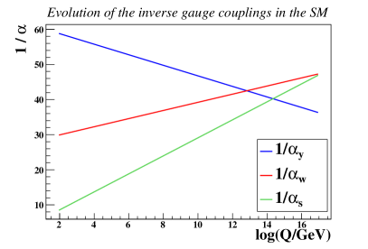
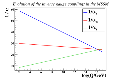
Figure 5.2: One-loop renormalization group evolution, as a function of the energy scale $Q$, of the inverse hypercharge ($\alpha_{y}^{-1}$), weak ($\alpha_{w}^{-1}$) and strong ($\alpha_{s}^{-1}$) gauge couplings in the Standard Model (left) and in the MSSM (right).

Starting from Eq. (4.3.5), the one-loop renormalization group equations for the hypercharge, weak and strong gauge coupling strengths $g_{y}$, $g_{w}$ and $g_{s}$ are given, when applied to the MSSM case, by

$$\begin{split}\frac{{\rm d}}{{\rm d}t}g_{y}=\frac{33}{80\pi^{2}}g_{y}^{3}\ ,\qquad\frac{{\rm d}}{{\rm d}t}g_{w}=\frac{1}{16\pi^{2}}g_{w}^{3}\qquad\text{and}\qquad\frac{{\rm d}}{{\rm d}t}g_{s}=-\frac{3}{16\pi^{2}}g_{s}^{3}\ .\end{split}$$ (5.2.10)

The evolution variable is taken as $t=\log(Q/Q_{0})$, where $Q_{0}$ is the scale at which the associated boundary conditions are imposed. Since the experimental measurements at the $Z$-boson scale allows for extracting very precisely the gauge couplings, $Q_{0}$ is in general chosen equal to $M_{Z}$. In contrast, in the Standard Model, the gauge couplings evolve according to

$$\begin{split}\frac{{\rm d}}{{\rm d}t}g_{y}=\frac{41}{160\pi^{2}}g_{y}^{3}\ ,\qquad\frac{{\rm d}}{{\rm d}t}g_{w}=-\frac{19}{96\pi^{2}}g_{w}^{3}\qquad\text{and}\qquad\frac{{\rm d}}{{\rm d}t}g_{s}=-\frac{7}{16\pi^{2}}g_{s}^{3}\ .\\ \end{split}$$ (5.2.11)

In the two series of equations above, the normalization of the hypercharge coupling $g_{y}$ has been chosen as predicted by the grand unification of the MSSM (or Standard Model) gauge group into $SU(5)$ or $SO(10)$. In this setup, the electromagnetic coupling constant $e$ is related to the hypercharge and weak coupling constants through the sine and cosine of the weak mixing angle $\theta_{w}$,

$$e=g_{w}\sin\theta_{w}=\sqrt{\frac{3}{5}}g_{y}\cos\theta_{w}\ .$$ (5.2.12)

This specific choice for the normalization of $g_{y}$ is adequate to ensure that Tr$(T_{a}T_{b})=1/2\delta_{ab}$ for any pair $T_{a}$ and $T_{b}$ of generators of $SU(5)$ or $SO(10)$ in the fundamental representation, including the hypercharge operator. Fixing the boundary conditions at the $Z$-pole as

$$M_{Z}=91.1876\text{ GeV }\ ,\ \ \sin\theta_{w}^{2}=0.23361\ ,\ \ \alpha^{-1}=\frac{4\pi}{e^{2}}=127.934\ \ \text{and}\ \ \alpha_{s}=0.118\ ,$$ (5.2.13)

we show in Figure 5.2 the evolution of the three gauge coupling constants with the energy. The Standard Model predictions of Eq. (5.2.11) are given in the left panel of the figure, while the MSSM results driven by the differential equations of Eq. (5.2.10) are presented in its right panel. In the MSSM, the three gauge couplings appear to unify at a scale of the order of $2\cdot 10^{16}$ GeV, in contrast to the Standard Model where no unification occurs. This value for the unification scale can be possibly seen as a hint favoring grand unified theories, which in general accommodate gauge coupling unification below the Planck scale.

The results presented in Figure 5.2 do not illustrate directly the evolution of the gauge coupling strengths $g_{i}$ (with $i=y$, $w$ and $s$) but rather exploit the one of the inverse of the quantities $\alpha_{i}=g_{i}^{2}/(4\pi)$. This is motivated by the fact that from Eq. (5.2.10) and Eq. (5.2.11), the $\alpha_{i}$ coupling constants are found to have the convenient property to run linearly with the renormalization group scale at the first order.

All these results can be extended to (and hold at) the two-loop level after also possibly including mass thresholds for the superpartners [248]. In this section, we however restrict ourselves to an illustration of the main phenomenological features of the MSSM and rather refer to public packages such as SPheno [249, 250], SuSpect [251] or SoftSusy [252, 253, 254] concerning results beyond the one-loop level.

5.2.3 Consequences of $R$-parity conservation

Imposing the conservation of $R$-parity, whose associated quantum number is obtained from Eq. (5.1.13), has important phenomenological consequences. First, the superpartners (sfermions, gauginos and higgsinos) are $R$-parity odd particles,

$$\begin{split}&R(\widetilde{H}_{u})=R(\widetilde{H}_{d})=R(\widetilde{B})=R(\widetilde{W})=R(\widetilde{g})=-1\ ,\\ &R(\tilde{q}_{L})=R(\tilde{u}_{R})=R(\tilde{d}_{R})=R(\tilde{\ell}_{L})=R(\tilde{e}_{R})=-1\ ,\end{split}$$ (5.2.14)

flavor indices being understood, while the particles of the Standard Model sector (quarks and leptons, gauge and Higgs bosons) are $R$-parity even states,

$$\begin{split}&R(H_{u})=R(H_{d})=R(B)=R(W)=R(g)=+1\ ,\\ &R(q_{L})=R(u_{R})=R(d_{R})=R(\ell_{L})=R(e_{R})=+1\ .\end{split}$$ (5.2.15)

Next, the exact conservation of $R$-parity implies that no particle mixing occurs between the Standard Model particles and their superpartners, as already shown in Section 5.1.4. In contrast, $R$-parity violating superpotential contributions such as the bilinear term of Eq. (5.1.12) leads to important mixings among the neutral particles of the spectrum (neutrinos and neutralinos; sneutrinos and neutral Higgs bosons) as well as among their charged counterparts (charged leptons and charginos; charged Higgs bosons and charged sleptons).

Furthermore, $R$-parity conservation imposes that each interaction vertex always involves an even number of $R$-parity-odd particles. Consequently, each superparticle always decays into an odd number of other, lighter, superparticles. The lightest supersymmetric particle is thus stable since all possible decay channels are kinematically closed. In addition, if this state is electrically and color neutral, it can be seen as an attractive candidate to explain the presence of non-baryonic dark matter in the universe [40, 41].

From the point of view of collider experiments, supersymmetric particles are always produced in pairs and each of the produced particles further decays following a possibly complicated chain where the latest link consists of the lightest supersymmetric particle, forming cascade decays [255, 256, 257, 258]. Moreover, once produced (either directly or from the decays of heavier superparticles), the lightest superpartner escapes the detector invisibly, which brings us to the typical supersymmetric signatures searched for at colliders, consisting of final states containing a fair amount of missing transverse energy produced in association with a possibly large number of jets and charged leptons.

5.3 Constraints from low-energy and electroweak precision measurements

Apart from direct searches at colliders, supersymmetric scenarios can be indirectly constrained by means of numerous low-energy and electroweak precision measurements restricting the masses and mixings of the superpartners. We dedicate this section to the study of the most stringent of these constraints and translate their effects in terms of parameter space scans in the context of the three supersymmetry-breaking scenarios presented in Section (5.1.5), i.e., the constrained version of the MSSM with four parameters and a sign (see Eq. (5.1.66)), the MSSM with gauge-mediated supersymmetry breaking described by four parameters and a sign (see Eq. (5.1.68)) and the MSSM with anomaly-mediated supersymmetry-breaking modeled by three parameters and a sign (see Eq. (5.1.69)).

5.3.1 Rare $B$-meson decays

Flavor physics observables are in general very sensitive to new physics, the associated measurements being one of the most promising ways to indirectly probe beyond the Standard Model effects. In particular, rare $B$-meson decays are already loop-suppressed in the Standard Model so that new physics diagrams are expected to contribute with the same order of magnitude.

The framework traditionally employed to compute theoretical predictions for $B$-physics observables consists of a low-energy heavy-quark effective field theory described by the Hamiltonian [259]

$$\mathcal{H}_{\rm eff}=-2\sqrt{2}G_{F}\ (V_{\rm CKM})_{ts}^{\ast}\ (V_{\rm CKM})_{tb}\ \sum_{i}{\cal C}_{i}(\mu_{b}){\cal O}_{i}(\mu_{b})\ ,$$ (5.3.1)

where $G_{F}$ is the Fermi constant. The most relevant effective operators ${\cal O}_{i}$ in the context of calculations related to $B$-decays depend on the electromagnetic and strong coupling constants $e$ and $g_{s}$, on the pole mass of the bottom quark $M_{b}$ and on the photon and gluon field strength tensors $F^{\mu\nu}$ and $g^{\mu\nu}$. Introducing in addition the fundamental representation matrices of the $SU(3)_{c}$ gauge group $T^{a}$, these operators read, employing four-component notations for the fermionic fields,

$$\begin{split}{\cal O}_{7}=&\ \frac{eM_{b}}{16\pi^{2}}{\bar{s}}_{L}\gamma_{\mu\nu}b_{R}F^{\mu\nu}\ ,\qquad\tilde{\cal O}_{7}=\frac{eM_{b}}{16\pi^{2}}{\bar{s}}_{R}\gamma_{\mu\nu}b_{L}F^{\mu\nu}\\ {\cal O}_{8}=&\ \frac{g_{s}M_{b}}{16\pi^{2}}{\bar{s}}_{L}\gamma_{\mu\nu}T^{a}b_{R}g^{\mu\nu}_{a}\ ,\qquad\tilde{\cal O}_{8}=\frac{g_{s}M_{b}}{16\pi^{2}}{\bar{s}}_{R}\gamma_{\mu\nu}T^{a}b_{L}g^{\mu\nu}_{a}\ ,\\ {\cal O}_{9}=&\ \frac{e^{2}}{16\pi^{2}}\big{[}{\bar{s}}_{L}\gamma_{\mu}b_{L}\big{]}\big{[}{\bar{\ell}}\gamma^{\mu}\ell\big{]}\ ,\qquad{\cal O}_{10}=\frac{e^{2}}{16\pi^{2}}\big{[}{\bar{s}}_{L}\gamma_{\mu}b_{L}\big{]}\big{[}{\bar{\ell}}\gamma^{\mu}\gamma^{5}\ell\big{]}\ .\end{split}$$ (5.3.2)

In these expressions, we have explicitly indicated, as a subscript, the left-handed ($L$) or right-handed ($R$) chirality of the charm ($c$), strange ($s$) and bottom ($b$) quark fields instead of employing the chirality projectors $P_{L}$ and $P_{R}$. Moreover, we generically note a charge lepton field as $\ell$. Getting back to Eq. (5.3.1), the renormalization scale $\mu_{b}$ is conveniently chosen of order of the mass of the bottom quark $M_{b}$, which ensures that all large logarithmic terms which could appear in computations based on the Hamiltonian $\mathcal{H}_{\rm eff}$ are embedded in the Wilson coefficients ${\cal C}_{i}$.

In order to perform accurate and reliable predictions, a calculation of the Wilson coefficients beyond the leading order in QCD is mandatory. In the framework of the MSSM, these quantities are known up to two loops with respect to QCD radiative corrections [260, 261] and up to one loop when including supersymmetric particles [262, 263, 264, 265, 266, 267, 268, 269]. Under that setup, the theoretical uncertainties are under good control and found to be reduced to a level of about $10\%$ [270, 271]. The MSSM predictions obtained in that way can be confronted to experimental data in order to extract constraints on the squark, chargino, neutralino and gluino masses and couplings. More generally, these bounds can be translated in terms of limits on the reduced set of model parameters associated with the supersymmetry-breaking scenarios.

The inclusive branching ratio BR($b\to s\gamma$) has been determined from combined measurements of the BABAR, BELLE, and CLEO experiments [272] and reads

$${\rm BR}(b\to s\gamma)=\big{(}3.55\pm 0.24_{\rm exp}\pm 0.23_{\rm theo}\big{)}\times 10^{-4}\ ,$$ (5.3.3)

where the theoretical uncertainties have been chosen according to the discussions presented in Ref. [273] and Ref. [274]. Possible contributions arising from supersymmetric diagrams have however been ignored. For these reasons, the ranges employed in the analysis of this section are estimated at the $2\sigma$ level, both for this observable as well as for any other of the observables presented below. In the context of a more general version of the MSSM where non-minimal $6\times 6$ squark mixings are allowed (see Eq. (5.1.63)), this measurement represents one of the most stringent constraints on the second and third generation mixing parameters in many popular supersymmetry-breaking mechanisms [135, 136, 137]. A second important observable consists of the $b\to s\mu^{+}\mu^{-}$ branching fraction, experimentally measured as [272]

$${\rm BR}(b\to s\mu^{+}\mu^{-})=\big{(}2.23\pm 0.98_{\rm exp}\pm 0.11_{\rm theo}\big{)}\times 10^{-6}\ ,$$ (5.3.4)

where we have taken the theoretical uncertainty from the results presented in Ref. [275]. Finally, due to very recent experimental data, the $B_{s}^{0}$-meson decay rate to a muon-antimuon pair has also become a strong constraint on new physics, with a branching ratio given by [276],

$${\rm BR}(B_{s}^{0}\to\mu^{+}\mu^{-})=\Big{(}3.2^{+1.5}_{-1.2}\Big{)}\times 10^{-9}\ ,$$ (5.3.5)

where theoretical uncertainties are included in the errors. This measurement performed by the LHCb collaboration consists of the first evidence for the $B_{s}^{0}\to\mu^{+}\mu^{-}$ decay. Data has been found compatible with the Standard Model expectation, the order of magnitude of the branching fraction being explained by both a loop-suppression and a helicity-suppression associated with the small muon mass.

Other observables could also be employed to constrain new physics, such as the branching ratios BR$(B_{u}\to\tau\nu_{\tau})$ or BR$(B\to D\tau\nu_{\tau})$. However, either their predictions cannot be computed in an accurate fashion due to the uncertainties on the relevant model parameters, or the associated experimental analysis is rather complex, which lead to large errors on the measurements. Therefore, we focus from now on the three $B$-meson decay constraints given by Eq. (5.3.3), Eq. (5.3.4) and Eq. (5.3.5).

To compute these observables in the context of the supersymmetry-breaking mechanisms of Section 5.1.5, our procedure starts at a high-energy scale with the few input parameters given either in Eq. (5.1.66), Eq. (5.1.68) or Eq. (5.1.69). The soft supersymmetry-breaking terms at the electroweak scale are then obtained through renormalization group running using the SPheno package version 3.2.1 [250], which solves the renormalization group equations numerically to two-loop order (see Section 4.3). This program next extracts the particle spectrum and mixings at the electroweak scale including one-loop corrections to the mass matrices of matter and gauge fields [235] and both one-loop and two-loop contributions to the Higgs mass matrices [233, 234, 277, 278, 279, 280, 281]. Finally, it computes several flavor physics observables, and in particular the branching ratio associated with the inclusive $b\to s\gamma$ decay [264, 265, 269], the one related to the inclusive $b\to s\mu^{+}\mu^{-}$ decay [264, 265, 267] and the exclusive branching ratio BR$(B_{s}^{0}\to\mu^{+}\mu^{-})$ [264, 263, 266].

For the numerical values of the Standard Model parameters, we fix the top quark pole mass to $M_{t}=173.5$ GeV, the bottom quark mass to $M_{b}(M_{b})=4.2$ GeV and the $Z$-boson mass to $M_{Z}=91.1876$ GeV. The Fermi constant has been taken as $G_{F}=1.16637\!\cdot\!10^{-5}$ GeV^-2, and the strong and electromagnetic coupling constants at the $Z$-pole as $\alpha_{s}(M_{Z})=0.1176$ and $\alpha(M_{Z})^{-1}=127.934$ [176]. Based on LHC searches with about 1 fb^-1 of data and on various sources of indirect constraints, benchmark planes for future searches on supersymmetry at the LHC have been defined from discussions among the supersymmetry working groups of the ATLAS and CMS experiments, together the LHC Physics Center at CERN [282]. For cMSSM scenarios, two $(m_{0},m_{1/2})$ planes have been proposed, motivated by the constraints derived from the measurements of the anomalous magnetic moment of the muon (see Section 5.3.3) and the rare $b\to s\gamma$ decay. Only models with a positive off-diagonal Higgs mixing parameter $\mu>0$ and $\tan\beta=10$, $A_{0}=0$ GeV or $\tan\beta=40$, $A_{0}=-500$ GeV have been adopted. While flavor bounds are not likely to strongly constrain regions of the parameter space with a low $\tan\beta$ value, loop-induced flavor-changing couplings of the Higgs bosons of the MSSM are enhanced for large values of $\tan\beta$ so that important effects are expected in the $\tan\beta=40$ case.

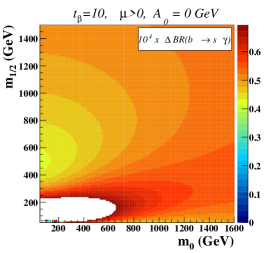
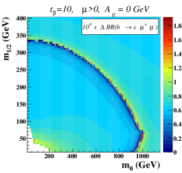
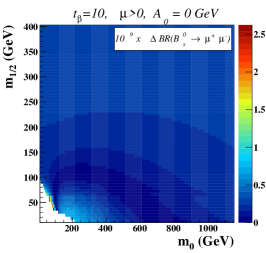
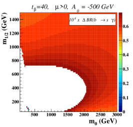
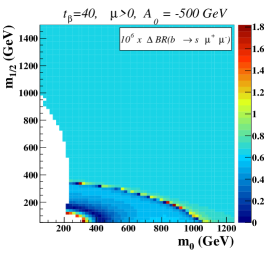
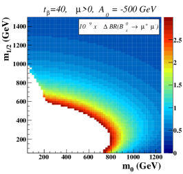
Figure 5.3: Theoretical predictions for the branching ratios associated with the inclusive $b\to s\gamma$ (left panel) and $b\to s\mu^{+}\mu^{-}$ (central panel) decays as well as with the exclusive $B_{s}^{0}\to\mu^{+}\mu^{-}$ decay given in terms of deviations from the central measured values given in Eq. (5.3.3), Eq. (5.3.4) and Eq. (5.3.5). We present the results in $(m_{0},m_{1/2})$-planes of the cMSSM for fixed values of $\tan\beta=10$, $A_{0}=0$ GeV and a positive Higgs mixing parameter $\mu>0$. The regions depicted in white correspond to excluded regions when applying the bounds of Eq. (5.3.3), Eq. (5.3.4) and Eq. (5.3.5) at the $2\sigma$-level, or to regions for which there is no solution to the supersymmetric renormalization group equations.

Figure 5.4: Same as Figure 5.4 but for fixed values of $\tan\beta=40$, $A_{0}=-500$ GeV and a positive Higgs mixing parameter $\mu>0$.

The theoretical predictions associated with the three $B$-physics observables discussed above are illustrated, for these two planes, on Figure 5.4 and Figure 5.4, respectively. In the left panel of the figures, we present theoretical predictions for the inclusive $b\to s\gamma$ branching ratio as deviations from the central value given in Eq. (5.3.3). In addition, we depict as white areas parameter space regions either excluded by the experimental limits of Eq. (5.3.3), imposed at the $2\sigma$-level, or for which there is no low-energy phenomenologically viable solution to the supersymmetric renormalization group equations.

For the two considered benchmark planes, the low-mass regions, even if attractive from a collider point of view, are strongly disfavored by indirect constraints derived from the measurement of the $b\to s\gamma$ branching ratio that is compatible with the Standard Model predictions. For relatively small values of $m_{0}$ and $m_{1/2}$, theoretical predictions are never found included in the $2\sigma$-range deduced from Eq. (5.3.3). Moreover, comparing results for $\tan\beta=10$ and $\tan\beta=40$, the constraints are found, as expected, enhanced for larger values of $\tan\beta$. The construction of viable, collider-friendly, benchmark scenarios with such a large $\tan\beta$ value is therefore challenging. Acceptable choices can however be made in two ways. The first option consists of keeping the gauginos relatively light (a small universal gaugino mass $m_{1/2}$) together with imposing the scalar particles of the model to be heavy (large universal scalar mass $m_{0}$ of several TeV). This allows for the heavy scalar propagators to tame the supersymmetric loop-diagram contributions to the $b\to s\gamma$ predictions, so that they lie well within the $2\sigma$-window derived from Eq. (5.3.3). The second option consists of fixing $m_{1/2}$ above one TeV, implying heavy gauginos that then reduce the supersymmetric effect on the $b\to s\gamma$ predictions for any value of $m_{0}$.

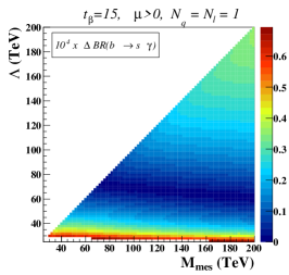
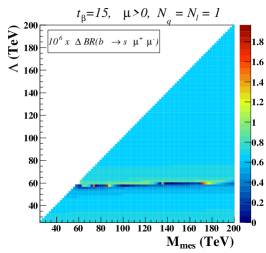
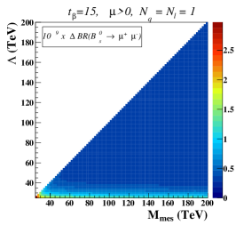
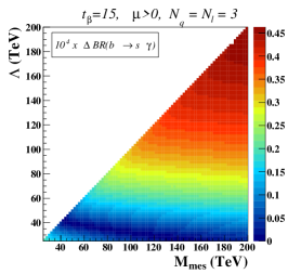
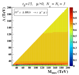
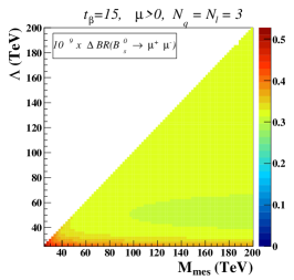
Figure 5.5: Same as Figure 5.4 but for gauge-mediated supersymmetry-breaking MSSM scenarios. We present $(M_{\rm mes},\Lambda)$ planes with $\tan\beta=15$, $N_{q}=N_{\ell}=1$ and a positive Higgs mixing parameter $\mu>0$.

Figure 5.6: Same as Figure 5.6 but for $N_{q}=N_{\ell}=3$.

The dependence of the $B$-physics observable on $\tan\beta$ is also illustrated on Figure 5.4 and Figure 5.4 in the context of the $b\to s\mu^{+}\mu^{-}$ (central panel) and $B_{s}^{0}\to\mu^{+}\mu^{-}$ decays (right panel), where we present the two branching ratios as deviations with respect to the central value of Eq. (5.3.4) and Eq. (5.3.5), respectively. The regions excluded at the $2\sigma$-level, as well as those for which there is no solution to the supersymmetric renormalization group equations, are again shown as white areas. For the case $\tan\beta=10$ and $A_{0}=0$ GeV (Figure 5.4), the effects of the supersymmetric contributions to these two observables are found to be numerically reduced due to the low value of $\tan\beta$. Additionally, both experimental measurements are suffering from large uncertainties. Consequently, the constraints on the parameter space are not competitive with those induced by the $b\to s\gamma$ observable.

In contrast, for larger values of $\tan\beta$, loop-corrections involving the bottom Yukawa coupling are enhanced so that the associated diagrams become as important as those involving the top Yukawa coupling. Enhancements of several orders of magnitude are in this way possible for the predictions of the BR$(B_{s}^{0}\to\mu^{+}\mu^{-})$ observable [283, 284]. The case $\tan\beta=40$ is illustrated on Figure 5.4. The constraints derived from the $b\to s\mu^{+}\mu^{-}$ and $B_{s}^{0}\to\mu^{+}\mu^{-}$ branching ratios are found not as restrictive as those induced by the inclusive $b\to s\gamma$ decay.

We now turn to the investigation of the MSSM with gauge-mediated supersymmetry breaking. In Ref. [282], two benchmark $(M_{\rm mes},\Lambda)$ planes have been adopted, with a fixed value of $\tan\beta=15$ and a positive $\mu$-parameter. The difference between the two planes lies in the number of messenger fields. In the first case, the model is constructed on the basis of $N_{q}=N_{\ell}=1$ messenger field while in the second case, it incorporates three sets of messengers ($N_{q}=N_{\ell}=3$). These two choices imply two different natures for the next-to-lightest superpartner, the lightest supersymmetric particle being always the gravitino. The next-to-lightest supersymmetric particle is hence the lightest stau for $N_{q}=N_{\ell}=3$ and the lightest neutralino for $N_{q}=N_{\ell}=1$.

The predictions for the three considered $B$-physics observables are presented on Figure 5.6 and Figure 5.6 for the $N_{q}=N_{\ell}=1$ and $N_{q}=N_{\ell}=3$ benchmark planes, respectively. For the entire scanned regions, one gets agreement between theory and experiment for all three observables, which is not surprising since gauge-mediated supersymmetry breaking naturally solves the so-called supersymmetric flavor problem. Supersymmetry is here usually broken within a few orders of magnitude from the weak scale, whereas the unrelated flavor-breaking scale can be chosen much higher. Consequently, the important flavor-violating terms included in the soft supersymmetry-breaking Lagrangian of Eq. (5.1.56) are avoided and one obtains, after diagonalization of the fermion sector, approximately flavor-conserving scalar mass matrices. Good agreement with measurements of flavor-changing neutral current observables is therefore foreseen, as shown in Figure 5.6 and Figure 5.6. Finally, the regions with $\Lambda>M_{\rm mes}$ are theoretically excluded as they do not allow for physical solutions of the supersymmetric renormalization group equations.

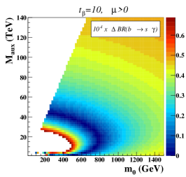
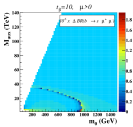
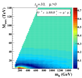
Figure 5.7: Same as Figure 5.4 but for anomaly-mediated supersymmetry-breaking MSSM scenarios. We present $(m_{0},M_{\rm aux})$ planes with $\tan\beta=10$ and a positive Higgs mixing parameter $\mu>0$.

In order to study the effect of the constraints derived from rare $B$-decays on MSSM scenarios where supersymmetry is broken via anomalies, we again follow the prescriptions of Ref. [282]. We adopt a benchmark plane inspired by the anomaly-mediated supersymmetry breaking benchmark point SPS9 [285]. The ratio of the expectation values of the two neutral Higgs boson is fixed to $\tan\beta=10$ and a positive sign for the $\mu$-parameter is chosen. The predictions for the three considered $B$-physics observables are presented in $(m_{0},M_{\rm aux})$ planes, in Figure 5.7, where we show, as above, their deviations from the central experimental values of Eq. (5.3.3), Eq. (5.3.4) and Eq. (5.3.5). As for the cMSSM, the low-mass regions with a relatively small $m_{0}$, attractive from a collider point of view, are strongly disfavored by data on the $b\to s\gamma$ branching ratio, the two other observables not bringing any additional restriction on the parameter space.

In the following, we turn to the investigation of the constraints induced by $B$-physics observables when more general squark mixings, like those given in Eq. (5.1.63), are allowed. We adopt a phenomenological approach where we assume non-negligible contributions to the off-diagonal terms of the squark soft mass matrices that we rewrite, in the super-CKM basis, as

$$M_{\tilde{q}}^{2}=\left(\begin{array}[]{ccc|ccc}M^{2}_{L_{q_{1}}}&\Delta^{q_{1}q_{2}}_{LL}&\Delta^{q_{1}q_{3}}_{LL}&X_{q_{1}}&\Delta^{q_{1}q_{2}}_{LR}&\Delta^{q_{1}q_{3}}_{LR}\\ \Delta^{q_{1}q_{2}\ast}_{LL}&M^{2}_{L_{q_{2}}}&\Delta^{q_{2}q_{3}}_{LL}&\Delta^{q_{1}q_{2}\ast}_{RL}&X_{q_{2}}&\Delta^{q_{2}q_{3}}_{LR}\\ \Delta^{q_{1}q_{3}\ast}_{LL}&\Delta^{q_{2}q_{3}\ast}_{LL}&M^{2}_{L_{q_{3}}}&\Delta^{q_{1}q_{3}\ast}_{RL}&\Delta^{q_{2}q_{3}\ast}_{RL}&X_{q_{3}}\\ \hline\cr X_{q_{1}}^{\ast}&\Delta^{q_{1}q_{2}}_{RL}&\Delta^{q_{1}q_{3}}_{RL}&M^{2}_{R_{q_{1}}}&\Delta^{q_{1}q_{2}}_{RR}&\Delta^{q_{1}q_{3}}_{RR}\\ \Delta^{q_{1}q_{2}\ast}_{LR}&X_{q_{2}}^{\ast}&\Delta^{q_{2}q_{3}}_{RL}&\Delta^{q_{1}q_{2}\ast}_{RR}&M^{2}_{R_{q_{2}}}&\Delta^{q_{2}q_{3}}_{RR}\\ \Delta^{q_{1}q_{3}\ast}_{LR}&\Delta^{q_{2}q_{3}\ast}_{LR}&X_{q_{3}}^{\ast}&\Delta^{q_{1}q_{3}\ast}_{RR}&\Delta^{q_{2}q_{3}\ast}_{RR}&M^{2}_{R_{q_{3}}}\end{array}\right)\ .$$ (5.3.6)

We have explicitly separated the left-left, left-right, right-left and right-right chiral sectors by means of horizontal and vertical line and additionally introduced shorthand notations for the flavor-diagonal elements,

$$\begin{split}M_{L_{u_{i}}}^{2}=(V_{\rm CKM}{\bf\hat{m}^{2}_{\tilde{Q}}}V_{\rm CKM}^{\dagger}\!+\!M_{q_{u}}^{2})^{i}{}_{i}\!+\!(\frac{1}{2}\!-\!\frac{2}{3}s_{w}^{2})c_{2\beta}M_{Z}^{2}\ ,&\quad M_{R_{u_{i}}}^{2}=({\bf\hat{m}^{2}_{\tilde{U}}}\!+\!M_{q_{u}}^{2})^{i}{}_{i}\!+\!\frac{2}{3}s_{w}^{2}c_{2\beta}M_{Z}^{2}\ ,\\ M_{L_{d_{i}}}^{2}=({\bf\hat{m}^{2}_{\tilde{Q}}}\!+\!M_{q_{d}}^{2})^{i}{}_{i}\!+\!(-\frac{1}{2}\!+\!\frac{1}{3}s_{w}^{2})c_{2\beta}M_{Z}^{2}\ ,&\quad M_{R_{d_{i}}}^{2}=({\bf\hat{m}^{2}_{\tilde{D}}}\!+\!M_{q_{d}}^{2})^{i}{}_{i}\!-\!\frac{1}{3}c_{2\beta}M_{Z}^{2}s_{w}^{2}\ ,\\ X_{u_{i}}=(\frac{v_{u}}{\sqrt{2}}{\bf\hat{T}^{u}}{}^{\dagger}-\frac{\mu}{\tan\beta}M_{q_{u}})^{i}{}_{i}\ ,&\quad X_{d_{i}}=(\frac{v_{d}}{\sqrt{2}}{\bf\hat{T}^{d}}{}^{\dagger}-\mu\tan\beta M_{q_{d}})^{i}{}_{i}\ .\end{split}$$ (5.3.7)

In these expressions, Einstein summation conventions are not applied on the generation index $i$. The off-diagonal parameters of the mass matrices that we denote by $\Delta$ are arbitrary and in general normalized to the diagonal entries of the soft supersymmetry-breaking mass matrices [286],

$$\Delta_{LL}^{u_{i}u_{j}}=\lambda^{u_{i}u_{j}}_{LL}({\bf\hat{m}^{2}_{\tilde{Q}}})^{i}{}_{i}({\bf\hat{m}^{2}_{\tilde{Q}}})^{j}{}_{j}\ ,\ \ \Delta_{LR}^{d_{i}d_{j}}=\lambda^{d_{i}d_{j}}_{LR}({\bf\hat{m}^{2}_{\tilde{Q}}})^{i}{}_{i}({\bf\hat{m}^{2}_{\tilde{D}}})^{j}{}_{j}\ ,\textit{etc.}\ .$$ (5.3.8)

Additional sources of squark flavor violation are then parametrized through the 21 dimensionless (possibly complex) new variables $\lambda^{q_{i}q_{j}}_{ab}$, recalling that the $\lambda_{LL}$ quantities for both the up-type and down-type squark sectors are identical. This also implies that both squark mass matrices cannot be simultaneously diagonal without neglecting the CKM matrix which we calculate using the Wolfenstein parametrization. The corresponding four free parameters are set to $\lambda_{\rm CKM}=0.2272$, $A_{\rm CKM}=0.818$, ${\bar{\rho}}_{\rm CKM}=0.221$ and ${\bar{\eta}}_{\rm CKM}=0.34$ [176].

Extensive studies of the kaon sector, $B$- and $D$-meson oscillations, rare decays, and electric dipole moments suggest that only flavor mixing involving the second and third generations of squarks can be substantial, and this only in the left-left and right-right chiral sectors [286, 287, 288, 289]. For this reason, we restrict to scenarios where only mixing of the second and third generation squarks is non-vanishing and that squarks with different chiralities can only mix in a flavor-conserving way. The only non-zero $\lambda$-parameters are thus given by

$$\lambda_{\rm L}\leavevmode\nobreak\ \equiv\leavevmode\nobreak\ \lambda_{LL}^{ct},\qquad\lambda_{R}\leavevmode\nobreak\ \equiv\leavevmode\nobreak\ \lambda_{RR}^{ct}=\lambda_{RR}^{sb}\ ,$$ (5.3.9)

in addition to $\lambda_{LL}^{sb}$ which is connected to $\lambda_{L}$ through the CKM matrix (see Eq. (5.3.7)). The equality $\lambda_{R}=\lambda_{RR}^{ct}=\lambda_{RR}^{sb}$ has been enforced for simplicity in order to avoid handling too many free parameters.

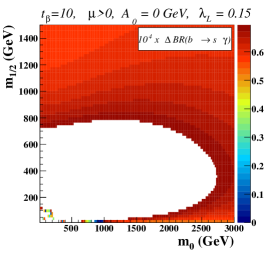
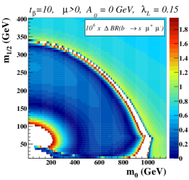
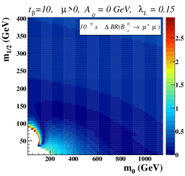
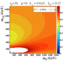
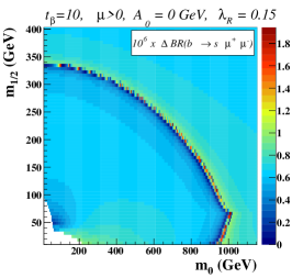
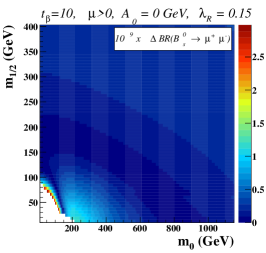
Figure 5.8: Same as in Figure 5.4 (cMSSM, $\tan\beta=10$, $A_{0}=0$ GeV, $\mu>0$) with $\lambda_{L}=0.15$.

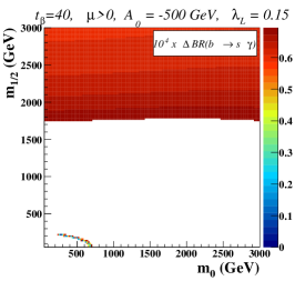
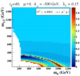
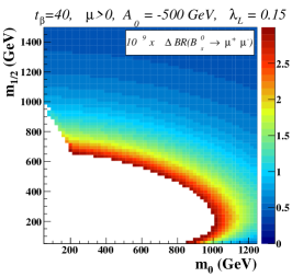
Figure 5.9: Same as in Figure 5.4 (cMSSM, $\tan\beta=10$, $A_{0}=0$ GeV, $\mu>0$) with $\lambda_{R}=0.15$.

Figure 5.10: Same as in Figure 5.4 (cMSSM, $\tan\beta=40$, $A_{0}=-500$ GeV, $\mu>0$) with $\lambda_{L}=0.15$.

We now revisit the previous studied constraints and address the phenomenology of MSSM scenarios including non-minimal flavor violation when the squark mass matrices are generalized by including the two flavor-violating parameters presented in Eq. (5.3.9) at low-energy. We however do not address the conception itself of fundamental mechanisms leading to non-vanishing flavor-violating squark mixing terms but provide instead several examples where such terms arise. In supergravity, they can be induced by non-trivial Kähler interactions. Although gauge-mediated supersymmetry-breaking scenarios are known to efficiently address the supersymmetric flavor problem, several possibilities for reintroducing flavor-violating terms have been pointed out recently [125, 290, 291]. For example, mixing between messenger and matter fields may lead to important flavor violation in the squark and slepton sectors. In Section 4.2.4, we have shown that in its simplest form, the mechanism yielding supersymmetry-breaking via anomalies leads to the problematics of tachyonic sleptons. In Section 5.1.5, we have presented a phenomenological approach to cure this problem by introducing additional and universal soft supersymmetry-breaking contributions to the scalar masses. This task could also be achieved in a non-universal way so that non-minimal flavor violation can be introduced in the theory [137].

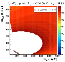
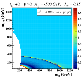
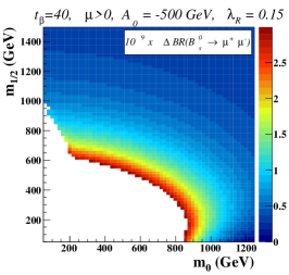
Figure 5.11: Same as in Figure 5.4 (cMSSM, $\tan\beta=40$, $A_{0}=-500$ GeV, $\mu>0$) with $\lambda_{R}=0.15$.

In Figure 5.10, Figure 5.10, Figure 5.10 and Figure 5.11, we depict the impact of the $\lambda_{L}$ and $\lambda_{R}$ parameters of Eq. (5.3.9) on the theoretical predictions for the three considered $B$-physics observables in the case of cMSSM scenarios with non-minimal flavor-violation. We adopt two scenarios, one where second and third generation squark mixing is only allowed in the left-left chiral sector ($\lambda_{L}=0.15$, $\lambda_{R}=0$) and one where it is only allowed in the right-right chiral sector ($\lambda_{R}=0.15$, $\lambda_{L}=0$). The $b\to s\gamma$ observable (left panel of the figures) allows us to probe non-minimally flavor-violating squark mixings in the left-left chiral sector through the effects of new flavor-violating loop-diagram contributions where lighter squark and (the wino component of the) neutralino or chargino fields propagate into the loops. Compared with the flavor-conserving case, larger fractions of the scanned $(m_{0},m_{1/2})$ planes are found to be excluded, so that phenomenologically viable scenarios imply heavier superpartners.

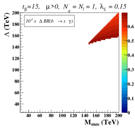
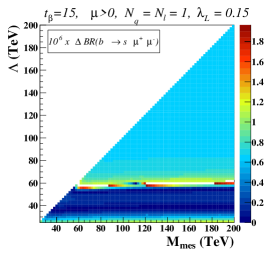
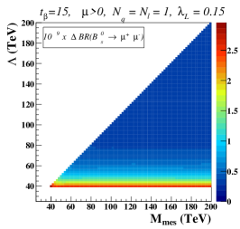
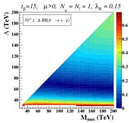
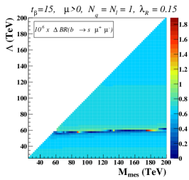
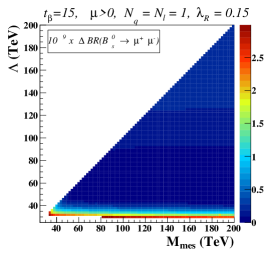
Figure 5.12: Same as in Figure 5.6 (MSSM with gauge-mediated supersymmetry breaking, $\tan\beta=15$, $N_{q}=N_{\ell}=1$, $\mu>0$) with $\lambda_{L}=0.15$.

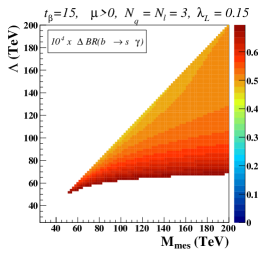
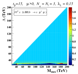
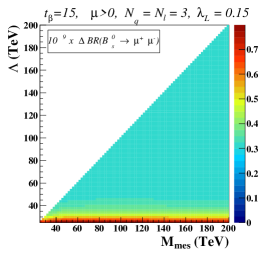
Figure 5.13: Same as in Figure 5.6 (MSSM with gauge-mediated supersymmetry breaking, $\tan\beta=15$, $N_{q}=N_{\ell}=1$, $\mu>0$) with $\lambda_{R}=0.15$.

Figure 5.14: Same as in Figure 5.6 (MSSM with gauge-mediated supersymmetry breaking, $\tan\beta=15$, $N_{q}=N_{\ell}=3$, $\mu>0$) with $\lambda_{L}=0.15$.

In contrast, the $b\to s\gamma$ branching ratio is insensitive to non-minimal right-right chiral squark mixings. The possible effects of a non-vanishing $\lambda_{R}$ parameter are related to the couplings of the higgsino component of the chargino and neutralino states and cMSSM scenarios usually imply lighter winos and heavier higgsinos, the associated $\lambda_{R}$-dependent contributions to the $b\to s\gamma$ branching ratio being thus suppressed.

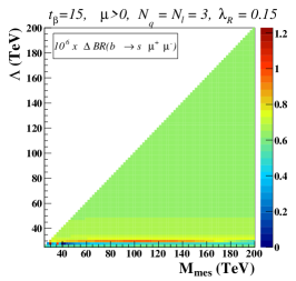
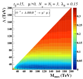
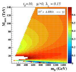
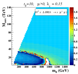
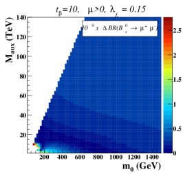
Figure 5.15: Same as in Figure 5.6 (MSSM with gauge-mediated supersymmetry breaking, $\tan\beta=15$, $N_{q}=N_{\ell}=3$, $\mu>0$) with $\lambda_{R}=0.15$.

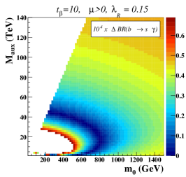
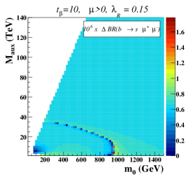
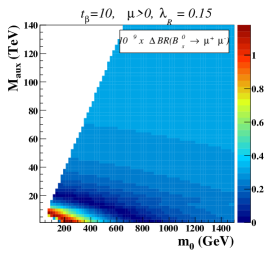
Figure 5.16: Same as in Figure 5.7 (MSSM with anomaly-mediated supersymmetry breaking, $\tan\beta=10$, $\mu>0$) with $\lambda_{L}=0.15$.

Figure 5.17: Same as in Figure 5.7 (MSSM with anomaly-mediated supersymmetry breaking, $\tan\beta=10$, $\mu>0$) with $\lambda_{R}=0.15$.

Non-minimal left-left squark chiral mixings also affect predictions for the $b\to s\mu^{+}\mu^{-}$ branching ratio (middle panels of the figures). All cMSSM regions regions excluded by $b\to s\mu^{+}\mu^{-}$ branching ratio measurements are however found to be also excluded by the $b\to s\gamma$ data. Contrary, right-right chiral mixings (right panels of the figures) cannot be probed, for the same reason as in the $b\to s\gamma$ case.

The large uncertainty on the $B_{s}^{0}\to\mu^{+}\mu^{-}$ branching ratio measurement potentially reduces the relevance of this observable to constrain squark flavor-violating mixings, in particular when confronting the constraining power of the $b\to s\gamma$ rare decay (see Figure 5.10, Figure 5.10, Figure 5.10 and Figure 5.11).

The same effects can be observed for gauge-mediated supersymmetry-breaking scenarios, as illustrated on Figure 5.14, Figure 5.14, Figure 5.14 and Figure 5.17, and for anomaly-mediated supersymmetry breaking MSSM scenarios as shown on Figure 5.17 and Figure 5.17. The theoretical predictions are insensitive to non-minimal flavor-violating right-right chiral mixings and the $b\to s\gamma$ branching ratio is the only observable capable to restrict the possibilities of constructing viable scenarios with non-minimal left-left chiral squark mixing.

5.3.2 $B$-meson oscillations

Weak interactions are responsible for providing different masses to the flavor eigenstates $|B_{q}^{0}\rangle=|{\bar{b}}q\rangle$ and $|{\bar{B}}_{q}^{0}\rangle=|b{\bar{q}}\rangle$, with $q=s$ or $d$, as well as mass mixing terms among those states. Consequently, the light ($L$) and heavy ($H$) neutral $B_{q}$-meson mass-eigenstates $|B_{q}^{L}\rangle$ and $|B_{q}^{H}\rangle$ differ in their masses and in their decay widths. Neglecting $CP$-violation since it is expected to be very small [292, 293, 294], the mass eigenstates are also $CP$-eigenstates, the light $|B_{q}^{L}\rangle$ state being $CP$-even and the heavy $|B_{q}^{H}\rangle$ state $CP$-odd. The evolution of a state prepared as a pure flavor eigenstate $|B_{q}^{0}\rangle$ or $|{\bar{B}}_{q}^{0}\rangle$ at a time $t=0$ is driven by the time-dependent probabilities ${\cal P}_{\rm unmix}(t)$ and ${\cal P}_{\rm mix}(t)$ that the flavor remains unchanged or oscillates,

$$\begin{split}{\cal P}_{\rm mix}(t)=&\ \frac{1}{2}\Gamma_{q}e^{-\Gamma_{q}t}\Big{[}1-\frac{\Delta\Gamma_{q}^{2}}{4\Gamma^{2}_{q}}\Big{]}\Big{[}\cosh\frac{\Delta\Gamma_{q}}{2}t-\cos\Delta M_{q}t\Big{]}\ ,\\ {\cal P}_{\rm unmix}(t)=&\ \frac{1}{2}\Gamma_{q}e^{-\Gamma_{q}t}\Big{[}1-\frac{\Delta\Gamma_{q}^{2}}{4\Gamma^{2}_{q}}\Big{]}\Big{[}\cosh\frac{\Delta\Gamma_{q}}{2}t+\cos\Delta M_{q}t\Big{]}\ ,\end{split}$$ (5.3.10)

respectively. In those expressions, $M_{q}$ and $\Gamma_{q}$ are the average mass and width of the $B_{q}$-mesons while $\Delta M_{q}$ and $\Delta\Gamma_{q}$ are the mass and width differences between the two eigenstates $|B_{q}^{L}\rangle$ and $|B_{q}^{H}\rangle$.

Among all the parameters introduced in Eq. (5.3.10), the mass difference $\Delta M_{s}$ is one of the key observables restricting the design of phenomenologically viable supersymmetric scenarios. The $B_{s}^{0}-{\bar{B}}_{s}^{0}$ oscillations have been observed for the first time in 2006 by the CDF and D0 collaborations [295, 296] and the precision on the measurement increases after the LHCb collaboration publishes results derived from the latest LHC data [297]. The oscillation frequency, given by the mass difference $\Delta M_{s}$, then reads [272]

$$\Delta M_{s}=\big{(}17.719\pm 0.043_{\rm exp}\pm 3.3_{\rm theo}\big{)}\text{ ps}^{-1}\ ,$$ (5.3.11)

where the theoretical uncertainty of 3.3 ps^-1 has been calculated in Ref. [298].

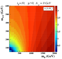
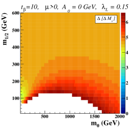
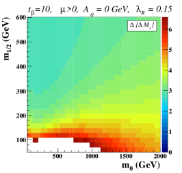
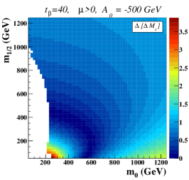
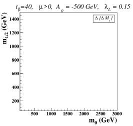
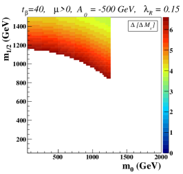
Figure 5.18: Predicted deviations from the central measured value for the mass difference between the two $B_{s}$-meson mass-eigenstates, as given in Eq. (5.3.11), in the framework of the cMSSM. We present the results in $(m_{0},m_{1/2})$-planes for fixed values of $\tan\beta=10$, $A_{0}=0$ GeV and a positive Higgs mixing parameter $\mu>0$. The regions depicted in white correspond to excluded regions when applying the bounds of Eq. (5.3.11) at the $2\sigma$-level, or to regions for which there is no solution to the supersymmetric renormalization group equations. Squark non-minimal flavor-violation is not allowed in the left panel of the figure, while we include non-vanishing flavor-violating squark mixing parameters $\lambda_{L}$ and $\lambda_{R}$ in its middle and right panels, respectively (see Eq. (5.3.9)).

Figure 5.19: Same as in Figure 5.19 but for $\tan\beta=40$, $A_{0}=-500$ GeV.

The computation of the associated theoretical predictions are based on the effective Hamiltonian of Eq. (5.3.1) and the four-fermion operators

$$\begin{split}{\cal O}_{1}^{q}=\big{[}{\bar{s}}_{L}\gamma_{\mu}T^{a}q_{L}\big{]}\big{[}{\bar{q}}_{L}\gamma^{\mu}T_{a}b_{L}\big{]}\ ,\quad&\ {\cal O}_{4}=\big{[}{\bar{s}}_{L}\gamma_{\mu}T^{a}b_{L}\big{]}\sum_{Q}\big{[}{\bar{Q}}\gamma^{\mu}T_{a}Q\big{]}\ ,\\ {\cal O}_{2}^{q}=\big{[}{\bar{s}}_{L}\gamma_{\mu}q_{L}\big{]}\big{[}{\bar{q}}_{L}\gamma^{\mu}b_{L}\big{]}\ ,\quad&\ {\cal O}_{5}=\big{[}{\bar{s}}_{L}\gamma_{\mu}\gamma_{\nu}\gamma_{\rho}b_{L}\big{]}\sum_{Q}\big{[}{\bar{Q}}\gamma^{\mu}\gamma^{\nu}\gamma^{\rho}Q\big{]}\ ,\\ {\cal O}_{3}=\big{[}{\bar{s}}_{L}\gamma_{\mu}b_{L}\big{]}\sum_{Q}\big{[}{\bar{Q}}\gamma^{\mu}Q\big{]}\ ,\quad&\ {\cal O}_{6}=\big{[}{\bar{s}}_{L}\gamma_{\mu}\gamma_{\nu}\gamma_{\rho}T^{a}b_{L}\big{]}\sum_{Q}\big{[}{\bar{Q}}\gamma^{\mu}\gamma^{\nu}\gamma^{\rho}T_{a}Q\big{]}\ ,\end{split}$$ (5.3.12)

with $q=u$ or $c$ dominantly contributing. The MSSM contributions to these operators have been calculated at the one-loop level in Ref. [264] and Ref. [266] and these results have been implemented in the computer code SPheno [250], which we employ to confront theory to data and constrain the MSSM parameter space.

In the context of the cMSSM, these constraints are translated in terms of scans of $(m_{0},m_{1/2})$ planes at fixed values of $\tan\beta$ and $A_{0}$. We refer to Section 5.3.1 for more details on the benchmark plane choices, and show, on Figure 5.19 and Figure 5.19, theoretical predictions for the mass difference $\Delta M_{s}$ associated with the $B_{s}$-meson system. These predictions are presented as deviations from the central value given in Eq. (5.3.11). Regions either excluded after imposing these constraints at the $2\sigma$-level, or for which there is no solution to the supersymmetric renormalization group equations linking high scale to low-energy scale physics, are depicted as white areas. In the case no squark non-minimal flavor violation is allowed (left panel of the figures), the large theoretical uncertainty of Eq. (5.3.11) strongly weakens the relevance of $\Delta M_{s}$ as a constraining observable for the construction of phenomenologically viable scenarios.

This contrasts with the case of scenarios featuring non-minimal flavor-violating mixings among the second and third generation squarks as defined in Eq. (5.3.9) (see the middle and right panels of Figure 5.19 and Figure 5.19). The $\Delta M_{s}$ observable is here highly sensitive to both mixings in the left-left chiral sector and in the right-right chiral sector as expected from the form of the dominant effective operators, contrary to $B$-meson rare decays which mainly probe mixings in the left-left chiral sector. Next, supersymmetric contributions to the $B_{s}^{0}-{\bar{B}}_{s}^{0}$ oscillations are strongly enhanced in parameter space regions where the value of $\tan\beta$ is large.

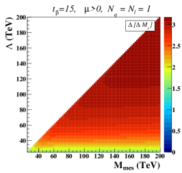
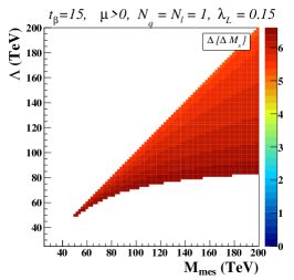
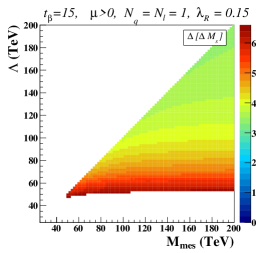
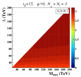
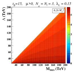
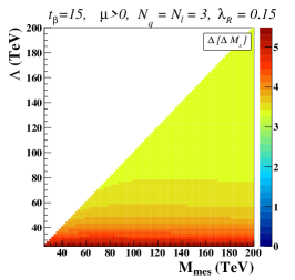
Figure 5.20: Same as in Figure 5.19 but for the MSSM with gauge-mediated supersymmetry-breaking. We present $(M_{\rm mes},\Lambda)$ planes with $\tan\beta=15$, one single series of messenger fields $N_{q}=N_{\ell}=1$ and a positive Higgs mixings parameter $\mu>0$.

Figure 5.21: Same as in Figure 5.19 but for the MSSM with gauge-mediated supersymmetry-breaking. We present $(M_{\rm mes},\Lambda)$ planes with $\tan\beta=15$, three series of messenger fields $N_{q}=N_{\ell}=3$ and a positive Higgs mixings parameter $\mu>0$.

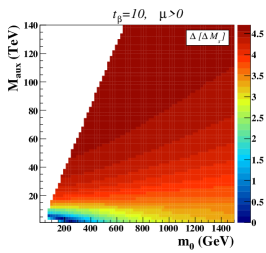
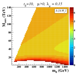
Figure 5.22: Same as in Figure 5.19 but for the MSSM with anomaly-mediated supersymmetry-breaking. We present $(m_{0},M_{\rm aux})$ planes with $\tan\beta=10$ and a positive Higgs mixing parameter $\mu>0$.

On Figure 5.21 and Figure 5.21, we turn to the case of the MSSM with gauge-mediated supersymmetry breaking and present $(N_{\rm mes},\Lambda)$ planes at fixed $\tan\beta$ and number of messenger fields. The investigated benchmark planes are those already described in Section 5.3.1 with $\tan\beta=15$ and $N_{q}=N_{\ell}=1$ or $N_{q}=N_{\ell}=3$. When flavor is conserved, i.e., when all $\lambda$-parameters of Eq. (5.3.9) are vanishing, good agreement is found between data and theory for the entire scanned regions after accounting for the large theoretical uncertainties. When allowing for non-minimal flavor violation, new constraints on the parameter space appear but are found to be less severe than those induced by rare $B$-meson decays (see Section 5.3.1).

Finally, we investigate MSSM scenarios with anomaly-mediated supersymmetry breaking on Figure 5.22, where $(m_{0},M_{\rm aux})$ planes at a fixed $\tan\beta=10$ value are presented. $B$-meson oscillations are found complementary to $B$-meson decays to constrain the parameter space in cases with non-minimal flavor violation in the squark sector, contrary to the MSSM with a flavor-conserving setup.

5.3.3 The anomalous magnetic moment of the muon

The world average experimental value for the muon anomalous magnetic moment is dominated by data collected by the E821 experiment at Brookhaven [299],

$$a_{\mu}^{\rm exp}=\big{(}11659208.0\pm 6.3\big{)}\times 10^{-10}\ .$$ (5.3.13)

Theoretical predictions in the Standard Model include QED contributions up to four loops and are even analytical up to the three-loop level [300, 301, 302, 303, 304, 305, 306, 307]. In addition, the leading logarithmic terms of the five-loop results are known [308, 309, 310, 311, 312, 313, 314, 315], as well as both the electroweak [316, 317, 318, 319, 320, 321, 322, 323, 324, 325, 326, 327] and hadronic contributions [328, 329] up to three loops. Moreover, the associated theoretical uncertainties are dominated by light-by-light scattering diagrams. The theoretical predictions hence read [176]

$$a_{\mu}^{\rm th}=\big{(}11659184.1\pm 4.8\big{)}\times 10^{-10}\ ,$$ (5.3.14)

which leads to a discrepancy of about $3\sigma$ between data and theory,

$$\Delta a_{\mu}=\big{(}23.9\pm 7.92\big{)}\times 10^{-10}\ ,$$ (5.3.15)

that we assume to be explained by new physics. In the context of supersymmetry, the dominant contributions $a_{\mu}^{\text{susy},1}$ to the anomalous magnetic moment of the muon consist of smuon, sneutrino, chargino and neutralino loops [330],

$$a_{\mu}^{\text{susy},1}\simeq 13\times 10^{-10}\Big{(}\frac{100\leavevmode\nobreak\ {\rm GeV}}{M_{\rm susy}}\Big{)}^{2}\tan\beta\ {\rm sign}(\mu)\ ,$$ (5.3.16)

where $M_{\rm susy}$ is a representative supersymmetry mass scale. This motivates the choice of a positive off-diagonal mixing $\mu$ parameter for all the considered benchmark scenarios as negative $\mu$-values would increase rather than decrease the discrepancy between data and theory.

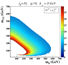
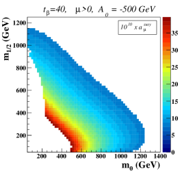
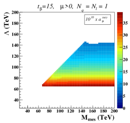
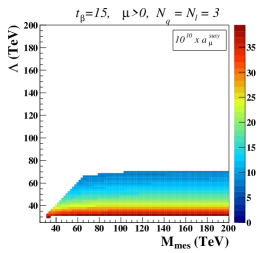
Figure 5.23: Supersymmetric contributions to the anomalous magnetic moment of the muon. Only the regions of the parameter space for which an agreement between the theoretical predictions and the measurements is found, at a $2\sigma$ level, are shown. We present the results in $(m_{0},m_{1/2})$-planes of the cMSSM for fixed values of $\tan\beta=10$ (40), $A_{0}=0$ GeV ($-500$ GeV) and a positive Higgs mixing parameter $\mu>0$ in the left (right) panel of the figure.

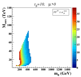
Figure 5.24: Same as in Figure 5.25 but for the MSSM with gauge-mediated supersymmetry-breaking. We present, in the left (right) panel of the figure, $(M_{\rm mes},\Lambda)$ planes for $\tan\beta=15$, one (three) single series of messenger fields $N_{q}=N_{\ell}=1$ (3) and a positive Higgs mixings parameter $\mu>0$.

Figure 5.25: Same as in Figure 5.25 but for the MSSM with anomaly-mediated supersymmetry-breaking. We present $(m_{0},M_{\rm aux})$ planes with $\tan\beta=10$ and a positive Higgs mixing parameter $\mu>0$.

We compute below the supersymmetric contributions to the muon anomalous magnetic moment including up to two-loop diagrams [331, 332, 333] and scan the parameter spaces associated with the three considered supersymmetry-breaking scenarios. In Figure 5.25, we show results in the cMSSM and demand that supersymmetry restores the agreement between theory and data within two standard deviations. We hence present parameter space regions compliant with this requirement for the two $(m_{0},m_{1/2})$ benchmark planes of the previous sections. Since squarks only contribute to the anomalous magnetic moment of the muon at the two-loop level, this considerably reduces the dependence of the $a_{\mu}$ on squark non-minimal flavor violation so that the results are independent of the considered $\lambda$-parameters.

Comparing with the results of Section 5.3.1 and Section 5.3.2, a significant fraction of the flavor-conserving cMSSM parameter space is found favored by both the $B$-physics constraints and the anomalous magnetic moment of the muon requirement, in particular for the small $\tan\beta$ region. Accommodating all constraints when non-minimal flavor violation is allowed becomes however challenging, as illustrated in the case of moderate left-left and right-right chiral squark mixings.

The same conclusions hold for MSSM scenarios with gauge-mediated supersymmetry-breaking, as shown on Figure 5.25 in which we present $(M_{\rm mes},\Lambda)$ benchmark planes for $\tan\beta=15$ and $N_{q}=N_{\ell}=1$ (left panel) and $N_{q}=N_{\ell}=3$ (right panel) messenger fields.

In contrast, it is very difficult to ask predictions of the anomalous magnetic moment of the muon to be compliant with data in the framework of MSSM scenarios with anomaly-mediated supersymmetry breaking, as illustrated on Figure 5.25. We show, by presenting theoretical results in a $(m_{0},M_{\rm aux})$ plane with $\tan\beta=10$, that only a very small part of the parameter space exhibits compatibility with experimental data. Imposing, in addition, constraints from $B$-physics (see previous sections) renders the design of viable benchmark scenarios complicated, as also found by other authors [334, 335]. Predictions for the anomalous magnetic moment of the muon are however strongly correlated to the slepton sector. The latter being linked to the way employed to solve the tachyonic slepton problem mentioned in Section 5.1.5, it is therefore convenient to ignore constraints from the anomalous magnetic moment of the muon when designing phenomenologically viable scenarios with anomaly-mediated supersymmetry breaking.

5.3.4 The electroweak $\rho$-parameter

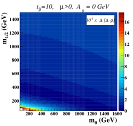
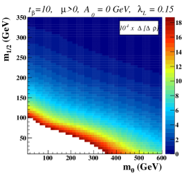
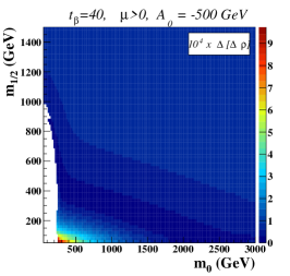
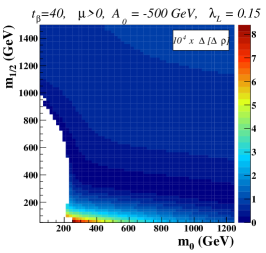
Figure 5.26: Supersymmetric contributions to electroweak precision observables given as deviations from the measured central value of the $\Delta\rho$ quantity defined in Eq. (5.3.18). We present the results in $(m_{0},m_{1/2})$-planes of the cMSSM with $\tan\beta=10$, $A_{0}=0$ GeV and a positive Higgs mixing parameter $\mu>0$. The regions depicted in white correspond to excluded regions when applying the bounds of Eq. (5.3.19) at the $2\sigma$-level, or to regions for which there is no solution to the supersymmetric renormalization group equations. Non-vanishing flavor-violating squark mixing parameters $\lambda_{L}$ and $\lambda_{R}$ are permitted in the middle and right panels of the figure, respectively (see Eq. (5.3.9)), while flavor violating squark mixing is forbidden in the left panel.

Figure 5.27: Same as in Figure 5.27 but for $\tan\beta=40$, $A_{0}=-500$ GeV.

Supersymmetry, as many extensions of the Standard Model, can be probed by means of electroweak precision observables such as the $\rho_{0}$-parameter. The latter is defined by

$$\rho_{0}=\frac{M_{W}^{2}}{M_{Z}^{2}\cos\theta_{w}^{2}\rho}\ ,$$ (5.3.17)

where the electroweak mixing angle $\theta_{w}$ is evaluated at the $Z$-pole and all loop effects are embedded into the $\rho$-parameter. For $\rho=\rho_{0}=1$, one recovers the well-known tree-level relation among the $Z$-boson and $W$-boson masses $M_{Z}$ and $M_{W}$. Eq. (5.3.17) provides a way to generalize this tree-level relation at higher orders [336, 337, 338, 339, 340]. In the Standard Model, the $\rho_{0}$-parameter is defined as equal to one, following the conventions of the Particle Data Group [176]. In contrast, for extensions of the Standard Model affecting the weak sector, $\rho_{0}$ usually differs from unity, the associated new physics contributions being more conveniently re-expressed as

$$\Delta\rho=\frac{\Sigma_{Z}(0)}{M_{Z}^{2}}-\frac{\Sigma_{W}(0)}{M_{W}^{2}}\ ,$$ (5.3.18)

where $\Delta\rho$ measures the deviation of the $\rho_{0}$ parameter from unity in terms of the weak vector boson self-energies at zero-momentum $\Sigma_{Z}(0)$ and $\Sigma_{W}(0)$. The $\Delta\rho$ quantity is traditionally employed to evaluate new physics contributions to electroweak precision observables such as the squared sine of the electroweak mixing angle or the $W$-boson mass. The latest combined fits of the $Z$-boson mass, width, pole asymmetry, $W$-boson and top-quark masses restrict $\Delta\rho$ to be in the range [176]

$$\Delta\rho=\big{(}1.564\pm 9.381\big{)}\times 10^{-4}\ .$$ (5.3.19)

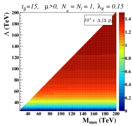
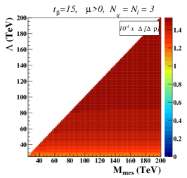
Figure 5.28: Same as in Figure 5.27 but for the MSSM with gauge-mediated supersymmetry-breaking. We present $(M_{\rm mes},\Lambda)$ planes with $\tan\beta=15$, one single series of messenger fields $N_{q}=N_{\ell}=1$ and a positive Higgs mixings parameter $\mu>0$.

Figure 5.29: Same as in Figure 5.27 but for the MSSM with gauge-mediated supersymmetry-breaking. We present $(M_{\rm mes},\Lambda)$ planes with $\tan\beta=15$, three series of messenger fields $N_{q}=N_{\ell}=3$ and a positive Higgs mixings parameter $\mu>0$.

In the context of the Minimal Supersymmetric Standard Model, radiative contributions to $\Delta\rho$ are known at the one-loop level [341]. Furthermore, the leading two-loop contributions involving gluonic loops as well as top and bottom Yukawa couplings have also been recently calculated [342, 343, 344, 345].

We present, in Figure 5.27 and Figure 5.27, theoretical predictions for the $\Delta\rho$ quantity of Eq. (5.3.18) in the framework of cMSSM scenarios as calculated by the SPheno program. We scan over the two considered $(m_{0},m_{1/2})$ benchmark planes ($\tan\beta=10$, $A_{0}=0$ GeV and $\tan\beta=40$, $A_{0}=-500$ GeV). By design, the $\Delta\rho$ parameter is directly sensitive to the mass splitting among the particles running into the loop-diagrams contributing to the self energies of the weak gauge bosons $\Sigma_{Z}$ and $\Sigma_{W}$. As shown in the left panel of the figures, the $\Delta\rho$ observable does not allow to extract constraints on the parameter space of the minimal models with $\lambda_{L}=\lambda_{R}=0$. However, when non-minimal flavor violation is included, the situation changes for the low $\tan\beta$ region (see the middle and right panels of the figures), the low-mass regions turning out to be excluded.

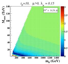
Figure 5.30: Same as in Figure 5.27 but for the MSSM with anomaly-mediated supersymmetry-breaking. We present $(m_{0},M_{\rm aux})$ planes with $\tan\beta=10$ and a positive Higgs mixing parameter $\mu>0$.

In Figure 5.29 and Figure 5.29, we explore MSSM scenarios with gauge-mediated supersymmetry-breaking and show scans of the $(M_{\rm mes},\Lambda)$ planes with $\tan\beta=15$ and respectively $N_{q}=N_{\ell}=1$ and $N_{q}=N_{\ell}=3$, while we address MSSM scenarios with anomaly-mediated supersymmetry breaking in Figure 5.30 in which we present $(m_{0},M_{\rm aux})$ planes for $\tan\beta\leavevmode\nobreak\ =\leavevmode\nobreak\ 10$. In all cases, almost all the scanned parameter space regions are found compatible with the measurements, so that this observable does not play a major role in constraining the construction of non-experimentally excluded benchmark scenarios.

5.3.5 Summary

In this section, we have investigated in details the MSSM effects on several low-energy, flavor and electroweak precision observables. We have considered, as a starting point for this study, two series of scenarios designed in the context of the cMSSM, two series of scenarios featuring gauge mediated supersymmetry breaking and one series of scenarios where supersymmetry gets broken via anomalies. Those scenarios have been chosen after relying on considerations of the LHC Physics Center at CERN and both the ATLAS and CMS collaborations after analyzing a fraction of the 2011 LHC data and a large class of indirect constraints on new physics.

Computing for each point predictions for several rare $B$-meson decays and the frequency of $B$-meson oscillations, it has been found that the low mass regions of the parameter space are in general excluded at the $2\sigma$ level in the cMSSM and anomaly-mediated supersymmetry-breaking cases, in contrast to gauge-mediated supersymmetry-breaking MSSM scenarios where supersymmetric contributions to those observables are reduced.

We have then started our exploration of non-minimal supersymmetric models and included non-minimal flavor violation in the squark sector for both left-left and right-right chirality mixings. We have shown that, especially for large flavor violation in the left-left sector, the constraints are much stronger than in the flavor-conserving case although large regions of the parameter space are still allowed by current flavor data.

We have next turned to electroweak constraints and calculated predictions for the anomalous magnetic moment of the muon. We have observed that there exist a substantial fraction of the parameter space for which supersymmetric loop diagrams allow to restore the agreement between theory and data. Contrary, current bounds on the $\rho$-parameter are not sufficient to induce any specific constraint at all, like when including non-minimal flavor violation in the squark sector.

5.4 Cosmological aspects

5.4.1 General features

Among the most compelling evidences for physics beyond the Standard Model is the presence of non-baryonic dark matter in the Universe. Its relic density is constrained to be, after combining seven-year data from WMAP with the latest measurements related to supernovæ, baryon acoustic oscillations and the Hubble constant [346],

$$\Omega_{\rm CDM}h^{2}=0.1126\pm 0.0036\ ,$$ (5.4.1)

where $h$ denotes the present Hubble expansion rate in units of 100 km s^-1 Mpc^-1. This value is however derived from an interpretation of cosmological data in the context of the six-parameter vanilla concordance model of cosmology.

In order for new physics theories to be compatible with such an observation, they must include a suitable dark matter candidate accounting for the quantity of dark matter given in Eq. (5.4.1). In the context of supersymmetry, we therefore require the lightest superpartner to be stable, electrically neutral and singlet under the QCD gauge group [40, 41]. Consequently, this motivates $R$-parity conservation and leaves the MSSM with three possible lightest supersymmetric particle, the lightest sneutrino, the lightest neutralino and the gravitino. However, phenomenologically viable scenarios with sneutrino dark matter are difficult to achieve by combining cosmological and collider constraints. On the one hand, a correct dark matter relic density can only be obtained if the lightest sneutrino is very light or very heavy, preventing from a too fast dark matter annihilation into Standard Model particles via $Z$-boson exchange diagrams [348, 349, 350]. On the other hand, very light sneutrinos are excluded by the invisible $Z$-boson width extracted at LEP [176] and very heavy sneutrinos are excluded by dark matter direct detection searches [350]. We therefore focus in this work on neutralino and gravitino dark matter scenarios.

5.4.2 Neutralino dark matter in the constrained MSSM

Being inspired by gravity-mediated supersymmetry-breaking, cMSSM scenarios include a gravitino field with a mass of the order of the TeV scale (see the relation among the different superpartner masses in Section (4.2.2)). The gravitino is therefore in general much heavier than some of the other superpartners and thus not a viable dark matter candidate. We consequently focus on neutralino dark matter. The energy density of a neutralino of mass $M_{\tilde{\chi}_{1}^{0}}$ is directly proportional to its present number density $n_{0}$,

$$\Omega_{\rm CDM}h^{2}=\frac{M_{\tilde{\chi}_{1}^{0}}n_{0}}{\rho_{c}}\ ,$$ (5.4.2)

where $\rho_{c}=3H_{0}^{2}/(8\pi G_{\rm N})$ is the critical density of our Universe, $G_{\rm N}$ being the gravitational constant and $H_{0}$ the present value of the Hubble expansion parameter [351]. The neutralino relic abundance $\Omega_{\rm CDM}h^{2}$ can be evaluated after solving the Boltzmann equation

$$\frac{{\rm d}n}{{\rm d}t}=-3Hn-\langle\sigma_{\rm eff}v\rangle\big{(}n^{2}-n_{\rm eq}^{2}\big{)}\ .$$ (5.4.3)

The first contribution to the right-hand side of this equation is proportional the time-dependent Hubble expansion parameter $H$ and describes a dilution of the dark matter density with the expansion of the Universe. On different footings, the second contribution is related to annihilations and co-annihilations of dark matter particles into Standard Model fermions and bosons. This term depends on the dark matter number density in thermal equilibrium $n_{\rm eq}$ as well as on the annihilation and co-annihilation effective cross section $\sigma_{\rm eff}$ multiplied by the relative particle velocity $v$. This product is then convoluted with the velocity distribution of the dark matter candidate to obtain the thermally averaged cross section $\langle\sigma_{\rm eff}v\rangle$. Taking into account a set of $N$ potentially co-annihilating superparticles, heavier than the lightest neutralino and with masses $M_{1}\leq\dots\leq M_{N}$, the thermally averaged cross section is given by [352, 353]

$$\langle\sigma_{\rm eff}v\rangle=\sum_{i,j=0}^{N}\langle\sigma_{ij}v_{ij}\rangle\frac{n_{\rm eq}^{i}n_{\rm eq}^{j}}{n_{\rm eq}^{2}}\ ,$$ (5.4.4)

where $n_{\rm eq}^{i}$ denotes the equilibrium number density of the particle $i$, the index $i=0$ referring to the lightest neutralino. We have also introduced the cross sections $\sigma_{ij}$ associated with the (co-)annihilation of the particles $i$ and $j$ and their relative velocity $v_{ij}$.

This last equation can be entirely rewritten in terms of the particle masses, the temperature $T$ and the number of internal degrees of freedom of each particle species $g_{i}$, or equivalently their statistical weights accounting for the number of possible combinations of related particle states,

$$\langle\sigma_{\rm eff}v\rangle=\sum_{i,j=0}^{N}\langle\sigma_{ij}v_{ij}\rangle\frac{g_{i}g_{j}}{g^{2}_{\rm eff}}\Big{[}\frac{M_{i}M_{j}}{M_{\tilde{\chi}_{1}^{0}}^{2}}\Big{]}^{3/2}\exp\Big{[}-\frac{(M_{i}+M_{j}-2M_{\tilde{\chi}_{1}^{0}})}{T}\Big{]}\ .$$ (5.4.5)

This expression depends in addition on the effective number of degrees of freedom $g_{\rm eff}$ that can be seen as an appropriate overall normalization factor. The mass differences between the superpartners hence play a crucial role in the computation of the relic density, the exponential suppression factor of Eq. (5.4.5) indicating that co-annihilations are only relevant for almost mass-degenerate superparticles.

In wide regions of the cMSSM parameter space, the annihilation of two neutralino states into Standard Model particles contributes dominantly to the computation of $\langle\sigma_{\rm eff}v\rangle$. However, other subprocesses could be significant. For instance, it is clear from Eq. (5.4.5) that non-trivial off-diagonal squark mixings that enhance splittings among the squark mass-eigenstates directly affect the predictions for the lightest neutralino relic density. In addition, flavor-violating couplings also imply that new channels could contribute to the effective annihilation and co-annihilation cross section. For example, annihilations of neutralinos into a charm-antitop or a top-anticharm quark pair become possible trough squark exchanges when the off-diagonal element of the squark mass matrices are of the same order as the diagonal ones [354].

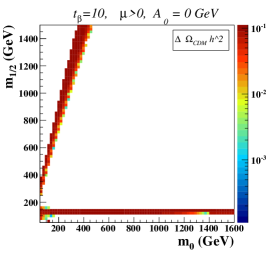
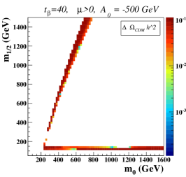
Figure 5.31: Theoretical predictions for the relic density of the lightest neutralino represented as deviations from the central value of Eq. (5.4.1). We present the results in $(m_{0},m_{1/2})$-planes of the cMSSM with $\tan\beta=10$, $A_{0}=0$ GeV (left) and $\tan\beta=40$, $A_{0}=-500$ GeV (right) and a positive Higgs mixing parameter $\mu>0$ in both case. The regions depicted in white correspond either to excluded regions when applying the upper bound of Eq. (5.4.1) at the $2\sigma$-level, to regions for which there is no solution to the supersymmetric renormalization group equations or to regions where the lightest neutralino is not the lightest supersymmetric particle (and therefore not a viable dark matter candidate).

In Figure 5.31, we present scans of the two cMSSM $(m_{0},m_{1/2})$ benchmark planes already introduced in Section 5.3 and show theoretical predictions for the neutralino dark matter relic density. After having firstly computed the particle masses and mixings by means of the SPheno package version 3.2.1 [250], the spectrum is in a second step exported to the DarkSusy code version 5.0.5 [355] which calculates the associated neutralino relic density. The regions depicted in white correspond either to regions for which there is no solution to the supersymmetric renormalization group equations, to regions where the lightest neutralino is not the lightest supersymmetric particle or to regions excluded after applying the upper bound of Eq. (5.4.1). This conservative assumption opens the possibility that either dark matter consists of several particle species, the lightest neutralino being only one of them, or that an alternative cosmological model is employed (see, e.g., Ref. [356, 357, 358, 359, 360, 361]). Regions of the parameter space compatible with the upper bound of Eq. (5.4.1) are indicated as colored areas, the color code being related to larger and larger deviations from the central value of Eq. (5.4.1). The entire scanned parameter space is found to be almost excluded by cosmological data.

Furthermore, it is important to note that a strict application of both the upper and lower limits of Eq. (5.4.1) leads to the exclusion of all the scanned parameter space, with the exception of the frontiers of the colored areas. Consequently, dark matter constraints turn out to be very hard to accommodate. In this case, allowing for non-minimal flavor violation does not help. Parameter space regions compliant with the observations are known to be rather insensitive to non-minimal flavor violation in the squark sector, the dominant diagrams being sub-dominant for moderate values of the $\lambda$-parameters of Eq. (5.3.9) [135]. One exception consists of fixing the $\lambda$-parameters to more extreme values, close to $\lambda=1$, as shown in Ref. [354].

The derivation of Eq. (5.4.1) has strongly relied on the assumption of the underlining cosmological model. The properties of the early Universe are however relatively unknown so that alternative cosmological models could be taken into account, such as models with a modified expansion rate [360, 361] or with a modified entropy content [361, 362]. Therefore, care must be taken when imposing dark matter constraints on the building of phenomenological models that could be reasonably evaded or modified.

5.4.3 Gravitino dark matter in gauge-mediated supersymmetry breaking

For MSSM scenarios where supersymmetry is broken through gauge interactions, the natural dark matter candidate is the gravitino. Depending on its mass, it can account either for cold ($m_{3/2}\gtrsim 100$ keV), warm ($1\ {\rm keV}\lesssim m_{3/2}\lesssim 100$ keV), or hot ($m_{3/2}\lesssim 1$ keV) dark matter. Two different sources contribute to the present gravitino abundance in the Universe,

$$\Omega_{\rm CDM}h^{2}=\Omega_{\rm CDM}^{\rm therm}h^{2}+\Omega_{\rm CDM}^{\rm non-therm}h^{2}\ .$$ (5.4.6)

The first contribution shows that gravitinos can be thermally produced in the very early Universe, the associated energy density reading [363, 364, 365]

$$\begin{split}\Omega_{\rm CDM}^{\rm therm}h^{2}\approx\Big{[}\frac{m_{3/2}}{100\ \text{GeV}}\Big{]}\Big{[}\frac{T_{R}}{10^{10}\ \text{GeV}}\Big{]}\sum_{i=1}^{3}\bigg{\{}\omega_{i}g_{i}^{2}\big{(}1+\frac{M^{2}_{i}}{3m^{2}_{3/2}}\big{)}\log\frac{k_{i}}{g_{i}}\bigg{\}}\ .\end{split}$$ (5.4.7)

The thermal contribution to the relic density $\Omega_{\rm CDM}^{\rm therm}$ involves, in addition to the gravitino mass $m_{3/2}$, a dependence on the reheating temperature $T_{R}$ which corresponds to the temperature of the Universe after inflation. No stringent constraints on $T_{R}$ exist, but values of the order ${\cal O}(10^{9})$ GeV and larger are preferred in scenarios that feature leptogenesis to explain the cosmic baryon asymmetry [366]. The summation included in Eq. (5.4.7) runs over the three gauge subgroups of the MSSM, i.e., $U(1)_{Y}$, $SU(2)_{L}$, and $SU(3)_{c}$ for which the couplings constants are denoted by $g_{i}$ and the soft mass parameters associated with the three gaugino fields by $M_{i}$. The constants $\omega_{i}$ and $k_{i}$ are taken as $\omega_{i}=0.018$, $0.044$, $0.117$ and $k_{i}=1.266$, $1.312$, $1.271$ for $i=1,2,3$, respectively, as in Ref. [364] where these values are derived from a consistent gauge-invariant finite-temperature calculation of all relevant squared matrix elements yielding gravitino production.

The second contribution to Eq. (5.4.6) consists of non-thermal production of gravitino through direct decays of the next-to-lightest supersymmetric particle into its Standard Model partner, together with a gravitino. The corresponding relic density $\Omega_{\rm CDM}^{\rm non-therm}$ depends on both the relic density of the next-to-lightest superparticle and its mass difference with the gravitino,

$$\Omega_{\rm CDM}^{\rm non-therm}h^{2}=\frac{m_{3/2}}{M_{\rm NLSP}}\Omega^{\rm therm}_{\rm NLSP}h^{2}\ .$$ (5.4.8)

The mass of the next-to-lightest superpartner is denoted by $M_{\rm NLSP}$ and its thermal relic density that would have been computed if it was stable by $\Omega^{\rm therm}_{\rm NLSP}h^{2}$. The would-be thermal relic density of the next-to-lightest supersymmetric particle $\Omega_{\rm NLSP}^{\rm therm}h^{2}$ is computed by solving the Boltzmann equation of Eq. (5.4.3) by means of the MicrOMEGAs package [367, 368, 369, 370, 371] since the DarkSusy program is only adapted for neutralino dark matter. Furthermore, we constrain the dark matter relic density as in Ref. [136],

$$0.094\leq\Omega_{\rm CDM}h^{2}\leq 0.136$$ (5.4.9)

at the $95\%$ confidence level. These numbers are extracted from three-year WMAP data, instead of seven-year WMAP data, and a non-minimal, more general, cosmological scenario with eleven parameters is assumed [372].

From Eq. (5.4.7) and Eq. (5.4.8), one observes that thermal gravitino production dominates for low values of the gravitino mass $m_{3/2}$ and/or a high reheating temperature $T_{R}$. In contrast, thermal production is found negligible for heavier gravitinos.

	$\Lambda$ [TeV]	$M_{\rm mes}$ [TeV]	$N_{q}=N_{\ell}$	$\tan\beta$	sign$(\mu)$	NLSP
E	65	90	1	15	$>0$	$\tilde{\chi}_{1}^{0}$
F	30	80	3	15	$>0$	$\tilde{\tau}_{1}$

Table 5.4: Benchmark MSSM scenarios featuring gauge-mediated supersymmetry breaking. We indicate, in addition to the value of the parameters of Eq. (5.1.68), the nature of the next-to-lightest superpartner (NLSP).

Extra constraints on scenarios with gravitino dark matter arise from the observed abundances of light elements in our Universe, which requires the next-to-lightest supersymmetric particle to decay fast enough [364]. Its lifetime $\tau_{\rm NLSP}$, given by the inverse of the total width, reads

$$\tau_{\rm NLSP}\approx 6100\ {\text{s}}\ \Big{[}\frac{1\ \text{TeV}}{M_{\rm NLSP}}\Big{]}^{5}\Big{[}\frac{m_{3/2}}{100\text{GeV}}\Big{]}^{2}\ ,$$ (5.4.10)

after neglecting any source of flavor violation and chirality mixings among sfermions, the latter having been found to have only little impact [135]. In order to ensure correct predictions for the abundances of the light elements as explained by primordial nucleosynthesis, the lifetime of the next-to-lightest supersymmetric particle has to satisfy the constraint $\tau_{\rm NLSP}\lesssim 6000$ s [373], favoring thus scenarios with a light gravitino.

In order to confront predictions for the gravitino relic density after imposing the constraint of Eq. (5.4.1) at the $2\sigma$ level, we select two representative benchmark scenarios among those included in the planes of Section 5.3. Following the conventions of Ref. [136], these scenarios are denoted by the letters E and F, and defined in Table 5.4.

The benchmark point E has been chosen in the region both favored by electroweak precision and flavor data (see Section 5.3). The superparticles are here rather light, the next-to-lightest supersymmetric particle being the lightest neutralino with a mass of $M_{\tilde{\chi}_{1}^{0}}=95.4$ GeV and the three lighter charged sleptons have close masses of about 100 GeV. The other sleptons, the sneutrinos, and the gauginos have moderate masses below 300 GeV, while squarks and gluino are quite heavy with masses above 700 GeV.

The point F is also compatible with low-energy and flavor constraints. In this case, the three lightest sleptons have masses of about 100 GeV, the next-to-lightest supersymmetric particle being the lightest stau with a mass $m_{\tilde{\tau}_{1}}=90.7$ GeV. The other sleptons, sneutrinos, and gauginos are a bit heavier but their masses are kept below 200 GeV. Finally, squarks and gluino have masses ranging up to 700 GeV.

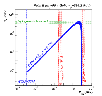
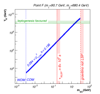
Figure 5.32: Cosmological constraints on the two MSSM scenarios with gauge-mediated supersymmetry breaking of Table 5.4 presented as $(m_{3/2},T_{R})$ planes. Regions favored by WMAP data are shown in blue, those predicting a correct lifetime for the next-to-lightest supersymmetric particle are indicated through a vertical red line and those favored by leptogenesis are shown by an horizontal green line. Regions where the gravitino consists of a warm (WDM) and cold (CDM) dark matter candidate are also pointed out, as well as those where the gravitino is not the lightest supersymmetric particle.

In Figure 5.32, we confront the predictions for the gravitino relic density after imposing the constraints of Eq. (5.4.1) and present the results in $(m_{3/2},T_{R})$ planes for the two benchmark scenarios E (left panel) and F (right panel). In both figures, we indicate the upper limit on the gravitino mass deduced from the lifetime of the next-to-lightest superpartner. The latter, computed as in Eq. (5.4.10), is asked to be shorter than 6000 seconds. In addition, the parameter space regions where the gravitino is a warm dark matter candidate, a cold dark matter candidate and not a suitable dark matter candidate are separated by means of vertical lines. Concerning the reheating temperature, we indicate the regions favored by leptogenesis, for which $T_{R}\gtrsim 10^{9}$ GeV.

The contributions to the gravitino relic density induced by decays of the next-to-lightest superparticle, $\Omega_{\rm CDM}^{\rm non-therm}h^{2}$, are only relevant for scenario E where the relic density of the lightest neutralino is rather large, $\Omega_{\rm NLSP}^{\rm therm}h^{2}=0.1275$. This value lying well within the interval favored by WMAP three-year data (see Eq. (5.4.9)), a band in the $(m_{3/2},T_{R})$ plane around $m_{3/2}\approx M_{\tilde{\chi}_{1}^{0}}=95.4$ GeV is found to be favored by the constraints. Concerning the benchmark point F, the lightest stau is the next-to-lightest superpartner and its annihilation cross section is large enough so that the corresponding relic density is negligible.

From the results shown in Figure 5.32, it is clear that all cosmological constraints cannot be fulfilled simultaneously. For instance, constructing a scenario featuring leptogenesis, i.e., where the reheating temperature is such that $T_{R}\gtrsim 10^{9}$ GeV, and predicting a correct value for the relic abundance leads to a too long predicted lifetime for the next-to-lightest superpartner so that light element abundances are spoiled. This property still holds for many other MSSM benchmark points with gauge-mediated supersymmetry breaking, as shown in Ref. [136]. However, the reheating temperature constraint, linked to leptogenesis, can in general be relaxed when building cosmologically viable MSSM scenarios. Mechanisms alternative to thermal leptogenesis can be accounted for to explain cosmic baryon asymmetry in the Universe, such as non-thermal leptogenesis via inflaton decay [374, 375] or Affleck-Dine leptogenesis [376]. We deduce from our results limits on an acceptable gravitino mass

$$10^{-4}\text{ GeV }\lesssim m_{3/2}\lesssim 0.1\text{ GeV }\ ,$$ (5.4.11)

which allows for gravitino cold dark matter whose relic density agrees with WMAP data. In addition, the next-to-lightest superparticle lifetime is kept short enough not to spoil light-element abundances.

5.4.4 Neutralino dark matter with anomaly-supersymmetry breaking

In MSSM scenarios where supersymmetry is broken through anomalies, the lightest of the four neutralinos is always the lightest superpartner and therefore a viable dark matter candidate. In contrast to the cMSSM, renormalization group evolution drives the wino mass parameter $M_{2}$ to a value smaller than the one of the two other gaugino mass parameters $M_{1}$ and $M_{3}$, dark matter being thus mostly wino-like. However, chargino masses also depend on the soft parameter $M_{2}$ so that the mass difference between the lightest neutralino and the lightest chargino is often of about a few GeV or less. From Eq. (5.4.5), it turns out that co-annihilations between these states are very efficient and play a significant role in the computations of predictions for the associated dark matter relic density.

$M_{\rm aux}$ [TeV]	$m_{0}$ [TeV]	$\tan\beta$	sign$(\mu)$	$M_{\tilde{\chi}^{0}_{1}}$ [GeV]	$M_{\tilde{\chi}^{\pm}_{1}}$ [GeV]
60	1	10	$>0$	174.5	174.7

Table 5.5: MSSM benchmark scenario featuring anomaly-mediated supersymmetry breaking. We indicate the supersymmetry-breaking parameters at the high scale (see Eq. (5.1.69)) and the masses, after renormalization group running, of the lightest neutralino and the lightest chargino.

As a result of a large co-annihilation cross sections, the neutralino relic density is usually, in anomaly-mediated supersymmetry-breaking scenarios, one or two orders of magnitude below the range given in Eq. (5.4.1) [377, 378]. We illustrate this feature by taking the specific example of one scenario of the scans of Section 5.3 that we define in Table 5.5. This scenario is compatible with constraints issued from flavor physics but do not include direct constraints on the masses of the superpartners (as in Section 5.4.3).

As a generic feature of MSSM scenarios with anomaly-mediated supersymmetry breaking, the lightest chargino and neutralino masses depend mainly on the auxiliary mass $M_{\rm aux}$, as shown in Eq. (4.2.54), and are roughly independent of the universal scalar mass $m_{0}$ introduced to solve the tachyonic slepton problem. After renormalization group running, these masses are found to be $M_{\tilde{\chi}^{0}_{1}}\sim M_{\tilde{\chi}^{\pm}_{1}}\sim 175$ GeV. Moreover, the larger value of the $m_{0}$ parameter leads masses above 1 TeV for the scalar superpartners and the gluino. Using the public code DarkSusy [355], we calculate the neutralino relic density $\Omega_{\rm CDM}h^{2}=8.57\times 10^{-4}$. As expected, this value is far too low compared the measurements (see Eq. (5.4.1)).

However, thermal production of neutralinos is not the only mechanism that has to be considered since in the context of anomaly-mediated supersymmetry breaking, several non-thermal production modes are possible. They include, for instance, the decay of heavy fields such as moduli, gravitinos, axions and axinos [378, 379, 380, 381]. In this work, we focus on two particular choices consisting first of decays of neutral scalar fields, called moduli fields $\Phi$, only coupling to matter via gravitational interactions and that are necessary for the UV completion of many phenomenologically-based models for cosmology, and secondly on gravitino fields.

The moduli contributions $\Omega_{\rm CDM}^{\rm mod}h^{2}$ to the neutralino relic density can be estimated as [382]

$$\Omega_{\rm CDM}^{\rm mod}h^{2}\approx 0.1\Big{[}\frac{M_{\tilde{\chi}^{0}_{1}}}{100\text{ GeV}}\Big{]}\ \Big{[}\frac{10.75}{g_{\rm eff}}\Big{]}^{1/4}\ \Big{[}\frac{3\cdot 10^{-24}\text{ cm}^{3}\text{s}^{-1}}{\langle\sigma_{\rm eff}v\rangle}\Big{]}\ \Big{[}\frac{100\text{ TeV}}{M_{\Phi}}\Big{]}^{3/2}\ .$$ (5.4.12)

The quantity $\Omega_{\rm CDM}^{\rm mod}$ depends on, in addition to the mass of the lightest neutralino $M_{\tilde{\chi}_{1}^{0}}$, the mass of the moduli fields $M_{\Phi}$, the effective number of degrees of freedom $g_{\rm eff}$ and the thermally averaged annihilation cross section $\langle\sigma_{\rm eff}v\rangle$. We present, in the left panel of Figure 5.33, isolines in the $(M_{\tilde{\chi}_{1}^{0}},M_{\Phi})$ plane where the neutralino relic density $\Omega_{\rm CDM}h^{2}=0.1126$ (as in Eq. (5.4.1)). These results assume an effective number of degrees of freedom equal to $g_{\rm eff}=10.75$ [378] and each curve is associated with a different value for the neutralino annihilation cross section $\langle\sigma_{\rm eff}v\rangle$. For the benchmark of Table 5.5, the neutralino mass is 175 GeV and the computed neutralino relic density reads $\Omega_{\rm CDM}h^{2}=8.57\times 10^{-4}$. This corresponds to a neutralino annihilation cross section of $\langle\sigma_{\rm eff}v\rangle\approx 10^{-23}$ cm³ s^-1. Consequently, constructing a scenario with moduli masses of order of $M_{\rm aux}=60$ TeV allows to recover the measured dark matter abundance of Eq. (5.4.1).

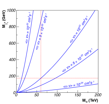
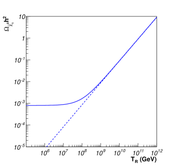
Figure 5.33: We present, in the left panel, curves defined by $\Omega_{\rm CDM}^{\rm mod}h^{2}=0.1126$ in the $(M_{\Phi},M_{\tilde{\chi}_{1}^{0}})$ plane for different values of the annihilation cross section $\langle\sigma v\rangle$. The dotted lines correspond to $M_{\tilde{\chi}^{0}_{1}}=175$ GeV and $M_{\Phi}=M_{\rm aux}=60$ TeV. In the right panel, we focus on the dependence on the reheating temperature $T_{R}$ of the neutralino relic density when both thermal and gravitino-induced non-thermal contributions are included (solid line) for the benchmark scenario of Table 5.5. In addition, the pure non-thermal contribution is indicated as a dashed line.

A second way to increase the neutralino relic abundance is to include contributions from gravitino decays,

$$\Omega_{\rm CDM}^{\rm non-therm}h^{2}=\frac{M_{\tilde{\chi}^{0}_{1}}}{m_{3/2}}\Omega_{3/2}h^{2}\ ,$$ (5.4.13)

where the gravitino thermal abundance $\Omega_{3/2}h^{2}$ is given as in Eq. (5.4.7). The mass ratio factor illustrates that each gravitino decays into one single stable neutralino. The corresponding effects are described on the right panel of Figure 5.33 for the scenario defined in Table 5.5 where we present the total neutralino relic density calculated as a function of the reheating temperature. For low values of $T_{R}$, thermal neutralino production dominates so that the total relic density, including both thermal and non-thermal contributions, has a roughly constant value of $\Omega_{\rm CDM}h^{2}\approx 8.57\times 10^{-4}$. When the reheating temperature reaches $10^{7}$ GeV, gravitino decays become dominant and the relic density grows linearly with $T_{R}$. Consequently, agreement with the observations corresponds to a reheating temperature of $T_{R}\approx 10^{10}$ GeV, a value in addition compatible with thermal leptogenesis [366].

5.5 Direct constraints

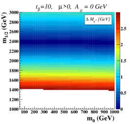
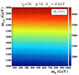
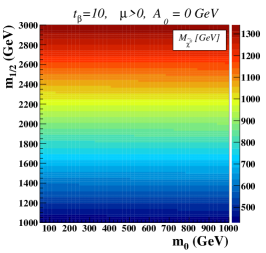
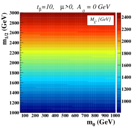
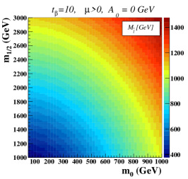
Figure 5.34: Predictions for the lightest Higgs boson mass (left panel, upper row) shown as deviations from the central measured value given in Eq. (5.5.1). We present the results in $(m_{0},m_{1/2})$-planes of the cMSSM with $\tan\beta=10$, $A_{0}=0$ GeV and a positive Higgs mixing parameter $\mu>0$. The predictions for the masses of the lightest squark (middle panel, upper row), the gluino (right panel, upper row), the lightest neutralino (left panel, lower row), the lightest chargino (middle panel, lower row) and the lightest slepton/sneutrino (right panel, lower row) are also depicted. In all figures, only the regions of the parameter space compatible with the bounds of Eq. (5.5.1) are indicated (1 TeV $<m_{1/2}<$ 3 TeV).

In the light of the latest experimental results, it is necessary to account for results of the direct searches of the Higgs boson [11, 12] when designing experimentally non-excluded scenarios. We therefore require

$$M_{h^{0}}\approx 126\pm 3\text{ GeV}\ ,$$ (5.5.1)

when scanning the MSSM parameter space. The central value is obtained from the average of the values reported by the two experimental collaborations and the bounds account for parametric uncertainties of the Standard Model inputs [383]. In Figure 5.34 and Figure 5.35, we scan over the two considered $(m_{0},m_{1/2})$ planes with $\tan\beta=10$, $A_{0}=0$ GeV and $\tan\beta\leavevmode\nobreak\ =\leavevmode\nobreak\ 40$, $A_{0}=-500$ GeV, respectively, and present, in the left panel of the upper row of the figures, predictions for the lightest Higgs boson mass shown as deviations from the central experimental value of 126 GeV. The theoretical computations are performed by means of the SPheno package, version 3.1.2, which includes one-loop and two-loop contributions to the Higgs mass matrices [233, 234, 277, 278, 279, 280, 281].

Confronting the Higgs mass predictions to data, it turns out that viable cMSSM scenarios prefer large values of the universal gaugino mass $m_{1/2}\gtrsim 1000$ GeV, while the universal scalar mass $m_{0}$ is left unconstrained. This has strong consequences on the superpartner spectrum, the predictions for their masses being presented in the other panels of Figure 5.34 and Figure 5.35 for the regions compatible with Eq. (5.5.1).

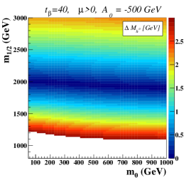
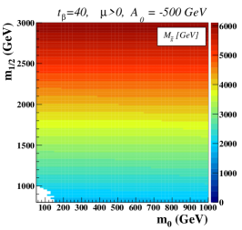
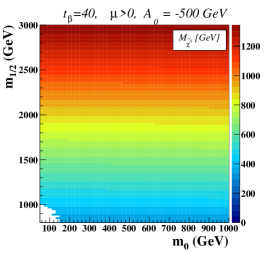
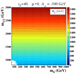
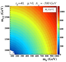
Figure 5.35: Same as Figure 5.34, but for $\tan\beta=40$, $A_{0}=-500$ GeV and a positive Higgs mixing parameter $\mu>0$.

In the middle panel of the upper row of the figures, we show the mass of the lightest of the squark eigenstates, i.e., the lightest stop. We observe that the regions of the scanned parameter space which accommodate $M_{h^{0}}\approx 126$ GeV also include heavy squarks of masses larger than 1 TeV. In this way, the tree-level Higgs mass of Eq. (5.1.36) is sufficiently shifted so that predictions agree with data. This however in general increases at the same time the amount of necessary fine-tuning as shown, e.g., by inspecting the logarithmic terms of Eq. (5.2.9). In the right panel of the figures, we show that these regions also exhibit heavy gluinos with masses above 2 TeV. Moreover, including non-minimal flavor violation as in Eq. (5.3.9) with $\lambda$-parameters equal to 0.15 does not induce enough mass splitting to drastically change the results. Although not considered in the examples studied in this work, lighter stop masses can still be viable to accomodate a correct Higgs boson mass. This specific setup requires an increased mixing among the two stop superpartners, or equivalently larger values of the $A_{0}$ parameter, and offers hence an alternative way for predicting a Standard Model-like Higgs boson with a mass of about 126 GeV and with a reduced amount of fine-tuning. We refer, e.g., to Refs. [384, 385] for more information.

On the second row of the figures (left and middle panels), we present predictions for the masses of the lightest neutralino and chargino in the regions accommodating a correct Higgs mass. These particles are expected to be lighter than squarks and gluino since the dominant effects driving the evolution of their masses with the energy are insensitive to the $SU(3)_{c}$ gauge interactions. The predicted masses are found to be above several hundreds of GeV for the lightest neutralino and above a TeV for the lightest chargino. Since the second lightest neutralino is mostly a wino state, as the lightest chargino, the range of its mass is can be inferred from the second panel of the second line of the figures. Finally, sleptons are in general the only superpartner to be allowed to be light, with masses of 100-200 GeV for large values of $\tan\beta$ being still possible. However, their possible discovery at the LHC is much more complicated. Either they can be observed through the cascade decays of strongly produced superparticles, or they are produced directly through the Drell-Yan mechanism. On the one hand, the first option is unlikely due to the heavy squark and gluino masses and the low cross sections [386, 387, 388, 389, 390, 391, 392, 393, 394, 395, 396, 397, 398, 399, 400, 401, 402]. On the other hand, direct production based searches rely on electroweak production processes [403, 404, 405, 406, 407, 408, 409, 410], whose cross sections are often found to be three or four orders of magnitude lower than those of the dominant $WW$ or $t\bar{t}$ backgrounds rendering the searches more challenging.

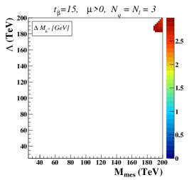
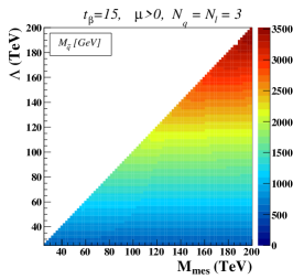
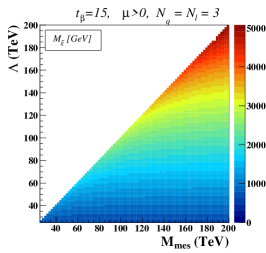
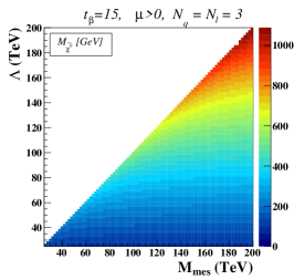
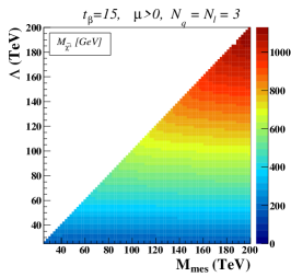
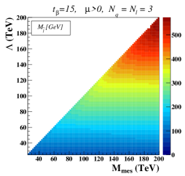
Figure 5.36: Same as in Figure 5.34 but for the MSSM with gauge-mediated supersymmetry-breaking. We present $(M_{\rm mes},\Lambda)$ planes with $\tan\beta=15$, $N_{q}=N_{\ell}=3$ messenger fields and a positive Higgs mixings parameter $\mu>0$.

Two remarks are in order here. First, all these predictions are compatible with the current experimental bounds induced by supersymmetry searches at the LHC experiments. With about 5 fb^-1 and 10 fb^-1 of data at a center-of-mass energy of 7 and 8 TeV, respectively, both the ATLAS and CMS collaborations have been able to set strong limits on low-scale supersymmetry. In particular, supersymmetry searches based on simplified models (often inspired by the cMSSM) and on the cMSSM itself stringently constrain the colored superpartner mass scale. Gluino and first and second generation squarks are currently pushed above 1 or 2 TeV [411, 412, 413, 414, 415, 416, 417, 418, 419, 420, 421, 422], while limits on third generation squark masses extend to about 500 GeV [419, 421, 422, 423, 424, 425, 426, 416, 427]. These negative search results have made the experimental attention shift towards the weak production channels, so that limits on chargino, neutralino and slepton masses have been improved to about 200-500 GeV [418, 420, 424, 428, 429, 430, 431]. Those limits are however not general and hold in very specific cases. Care should be taken when reinterpreted in different contexts such as a complete model, for instance.

The direct measurements are compatible with results extracted from flavor physics and electroweak precision data (see Section 5.3.1, Section 5.3.2 and Section 5.3.4), heavy superpartners being both favored by Higgs mass measurements and rare $B$-meson decays, neutral $B$-meson oscillations and electroweak precision observable data. However, scenarios with too heavy superparticle masses forbid supersymmetry to explain the gap between Standard Model predictions and measurements of the anomalous magnetic moment of the muon (see Section 5.3.3). Relaxing the $a_{\mu}$ constraints, viable benchmark scenarios can however be built, but are very collider-unfriendly with superpartners above the TeV range.

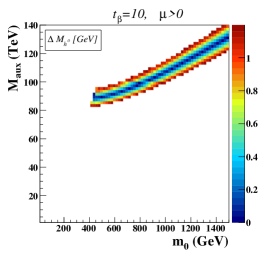
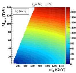
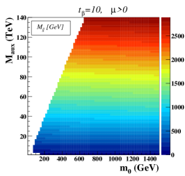
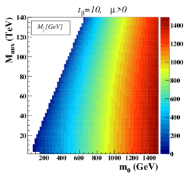
Figure 5.37: Same as in Figure 5.34 but for the MSSM with anomaly-mediated supersymmetry-breaking. We present $(m_{0},M_{\rm aux})$ planes with $\tan\beta=10$ and a positive Higgs mixing parameter $\mu>0$.

Turning to the MSSM with gauge-mediated supersymmetry-breaking, it is found that it is very difficult to accommodate the bounds on the Higgs mass of Eq. (5.5.1) for a large fraction of the parameter space. For instance, no scenario for which $\tan\beta=15$ and $N_{q}=N_{\ell}=1$ is compliant with the measurements. Even for $N_{q}=N_{\ell}=3$, the only way to restore agreement with data disfavors light supersymmetry (see Figure 5.36). The viable regions however also satisfies the indirect constraints of Section 5.3, with again the exception of the anomalous magnetic moment of the muon. Signatures of gauge-mediated supersymmetry-breaking scenarios are different from those expected in the context of the cMSSM. In particular, final states rich in photons are expected due to the different nature for the lightest superparticle. Dedicated experimental analyses have led to excluded mass ranges very similar to those excluded in the cMSSM framework [432, 433, 434, 435].

We finally present, in Figure 5.37, $(m_{0},M_{\rm aux})$ planes with $\tan\beta=10$ for MSSM scenarios with anomaly-mediated supersymmetry breaking. The Higgs mass predictions are shown in the left panel of the first row of the figure and the masses of the (lightest) superpartners in the rest of the figure. Only a narrow band of the scanned parameter space leads to an agreement with the Higgs mass measurement, but also predicts heavy superpartners of several TeV.

One important point to note is that in this region, the numerical value of the lightest Higgs boson mass returned by SPheno 3 differs by several GeV from those obtained by making use of SPheno version 2 [249], SuSpect [251] or SoftSusy [252, 253, 254], that all agree with each other. This difference is explained by consistently including in SPheno 3 gauge-invariant contributions to the Higgs mixing parameters $b$ and $\mu$ [436]. As a consequence, SPheno predictions show that anomaly-mediated supersymmetry breaking might still be viable, contrary to other spectrum generators predictions [383, 437]. Experimental analyses exclusively dedicated to anomaly-mediated supersymmetry-breaking scenarios exist, but only focus on the neutralino and chargino sectors. Weak constraints have been extracted on the chargino and neutralino mass required to be above ${\cal O}(100)$ GeV [438].

5.6 Motivation for going beyond the MSSM

In the previous sections, we have presented a representative set of constraints that can be employed when constructing theoretically motivated and not experimentally excluded benchmark scenarios. Direct searches at colliders (and in particular at the LHC), indirect constraints obtained from low-energy flavor and electroweak precision observables and cosmological data have been considered. We have concluded that it becomes very difficult to accommodate both light supersymmetry and all the constraints. Experimental results such as the discovery of a Higgs boson or the absence of any supersymmetric particle in current LHC data tend to show that if Nature is supersymmetric, supersymmetry lies above the TeV range. Viable regions are in general compatible with flavor and electroweak precision data, but are however not able to provide an explanation for the discrepancy between theory and experiment for the anomalous magnetic moment of the muon.

In order to reconcile supersymmetry, collider friendship and data, another option consists of leaving the minimal picture. We have already shown that allowing for non-minimal flavor violation in the MSSM can affect theoretical predictions. Moreover, current experimental results may not be valid in more general supersymmetric frameworks, in particular since most of all the current bounds are derived from simplified models inspired by the cMSSM. Although typical supersymmetric signatures, such as the presence of missing transverse energy in the final state, are common for the MSSM and many non-minimal supersymmetric models, dedicated phenomenological studies can be required to study new types of signatures. In the next chapter of this work, several non-minimal models are investigated, namely the MSSM with $R$-parity violation [138], $N\!=\!1\!/\!N\!=\!2$ hybrid supersymmetric theories [439, 440, 441, 442, 443, 444, 445, 446, 447] and minimal $R$-symmetric supersymmetric theories [139, 140, 141]. To this aim, we will make use of the tools introduced in Chapter 3 to perform LHC phenomenological studies based on Monte Carlo simulations.

Chapter 6 Searching for non-minimal supersymmetry at hadron colliders

As stated in Section 5.6, there are large classes of non-minimal supersymmetric theories valuable to be investigated. We choose to focus in this work on two of these, namely the MSSM with $R$-parity violation [138] and the minimal version of supersymmetric theories with an unbroken $R$-symmetry [139, 140, 141]. We first dedicate Section 6.1 to the description of the considered models and to the presentation of their main phenomenological implications. Next, Section 6.2 and Section 6.3 are more technical and show how to efficiently perform phenomenological LHC analyses in the framework of these models by means of Monte Carlo simulations. For the sake of the example, two analyses are finally addressed in Section 6.4 and Section 6.5.

6.1 Beyond minimal supersymmetry: two examples

6.1.1 $R$-parity violation

The conservation of $R$-parity is invoked to forbid the lepton-number-violating and baryon-number-violating interactions and mass terms induced by the superpotential contributions

$$\begin{split}W_{RPV}=\frac{1}{2}\lambda_{ijk}L_{L}^{i}\!\cdot\!L_{L}^{j}E_{R}^{k}+\lambda^{\prime}_{ijk}L_{L}^{i}\!\cdot Q_{L}^{j}D_{R}^{k}+\frac{1}{2}\lambda^{\prime\prime}_{ijk}U_{R}^{i}D^{j}_{R}D_{R}^{k}-\kappa_{i}L_{L}^{i}\!\cdot\!H_{U}\ ,\end{split}$$ (6.1.1)

and the soft supersymmetry-breaking Lagrangian

$$\begin{split}{\cal L}_{{\rm soft},RPV}=&\ \Big{[}D_{i}\tilde{\ell}_{L}^{i}\!\cdot\!H_{u}-({\bf m_{LH}^{2}})^{i}\tilde{\ell}_{Li}^{\dagger}H_{d}+{\rm h.c.}\Big{]}\\ &\ -\Big{[}\frac{1}{2}T_{ijk}\tilde{\ell}_{L}^{i}\!\cdot\!\tilde{\ell}_{L}^{j}\tilde{e}_{R}^{k{\dagger}}+T^{\prime}_{ijk}\tilde{\ell}_{L}^{i}\!\cdot\!\tilde{q}^{j}_{L}\tilde{d}_{R}^{k{\dagger}}+\frac{1}{2}T^{\prime\prime}_{ijk}\,\tilde{u}_{R}^{i{\dagger}}\tilde{d}_{R}^{j{\dagger}}\tilde{d}_{R}^{k{\dagger}}+{\rm h.c.}\Big{]}\ .\end{split}$$ (6.1.2)

In those equations, all indices but the flavor ones are understood and the notations for the superfields and their components are compliant with those introduced in Section 5.1.1. The parameters $\kappa$, $D$ and ${\bf m^{2}_{LH}}$ are three-dimensional vectors and $\lambda$, $\lambda^{\prime}$, ${\lambda^{\prime\prime}}$, $T$, $T^{\prime}$, $T^{\prime\prime}$ are $3\times 3\times 3$ tensors in generation space.

Switching to the super-CKM and super-PMNS basis, these parameters are redefined to prevent the rotation matrices of Eq. (5.1.51) and Eq. (5.1.52) to explicitly appear in the Lagrangian, having instead an explicit dependence on the CKM and PMNS matrices. This leads to the $R$-parity violating superpotential

$$\boxed{\begin{split}W_{RPV}=&\ (V_{\rm PMNS}^{\dagger})^{i}{}_{i^{\prime}}\hat{\lambda}_{ijk}N_{L}^{i^{\prime}}E_{L}^{j}E_{R}^{k}+(V_{\rm PMNS}^{\dagger})^{i}{}_{i^{\prime}}(V_{\rm CKM}^{\dagger})^{j}{}_{j^{\prime}}\hat{\lambda}^{\prime}_{ijk}L_{L}^{i^{\prime}}\!\cdot Q_{L}^{j^{\prime}}D_{R}^{k}\\ &\ +\frac{1}{2}\hat{\lambda}^{\prime\prime}_{ijk}U_{R}^{i}D^{j}_{R}D_{R}^{k}-\hat{\kappa}_{i}L_{L}^{i}\!\cdot\!H_{U}\ ,\end{split}}$$ (6.1.3)

and to the soft supersymmetry-breaking Lagrangian

$$\boxed{\begin{split}{\cal L}_{{\rm soft},RPV}=&\ \Big{[}\hat{D}_{i}\tilde{\ell}_{L}^{i}\!\cdot\!H_{u}-({\bf\hat{m}_{LH}^{2}})^{i}\tilde{\ell}_{Li}^{\dagger}H_{d}+{\rm h.c.}\Big{]}-\Big{[}(V_{\rm PMNS}^{\dagger})^{i}{}_{i^{\prime}}\hat{T}_{ijk}\tilde{\nu}_{L}^{i^{\prime}}\!\cdot\!\tilde{e}_{L}^{j}\tilde{e}_{R}^{k{\dagger}}\\ &\ +(V_{\rm PMNS}^{\dagger})^{i}{}_{i^{\prime}}(V_{\rm CKM}^{\dagger})^{j}{}_{j^{\prime}}\hat{T}^{\prime}_{ijk}\tilde{\ell}_{L}^{i^{\prime}}\!\cdot\!\tilde{q}^{j^{\prime}}_{L}\tilde{d}_{R}^{k{\dagger}}+\frac{1}{2}\hat{T}^{\prime\prime}_{ijk}\,\tilde{u}_{R}^{i{\dagger}}\tilde{d}_{R}^{j{\dagger}}\tilde{d}_{R}^{k{\dagger}}+{\rm h.c.}\Big{]}\ ,\end{split}}$$ (6.1.4)

the hatted parameters being used as input parameters according to the Supersymmetry Les Houches Accord conventions [175]. We have also introduced, in those expressions, the left-handed neutrino and left-handed charged lepton superfields $N_{L}$ and $E_{L}$, i.e., the components of the $SU(2)_{L}$ doublet $L_{L}$, and their scalar components $\tilde{\nu}_{L}$ and $\tilde{e}_{L}$. Whereas there is not any theoretical motivation to forbid these $R$-parity violating couplings terms, most of them are however highly constrained by experimental measurements.

The size of the lepton-number-violating operators is strongly restricted by the smallness of the neutrino masses [448, 449, 450, 451, 452], the neutrino oscillations rate along their propagation within media [453, 454] and the negative results from neutrinoless double beta decay searches [455, 456, 457, 458]. In addition, bounds on quadratic and quartic products of couplings are obtained from lepton rare decays [459, 460, 461], strange or $B$-meson decays [462, 460, 463, 464, 465], atomic parity violation data [466, 467] or magnetic and electric dipole moment measurements [468, 469, 470, 471, 472]. For superpartners with masses of the order of several hundreds of GeV, the lepton-number-violating couplings of Eq. (6.1.3) and Eq. (6.1.4) are typically constrained to be smaller than about $0.01-0.1$ [138, 473]. Indirect limits on the baryon-number-violating operators arise either from single nucleon decay data, and in particular from the proton lifetime measurements, [474, 475, 476, 477, 478, 479], from $K$-meson or $B$-meson data [480, 481, 482, 483, 484] or from nucleon-antinucleon oscillations and double nucleon decays [477, 485, 486]. However, the most restrictive bounds are implied by cosmology, the observed flux of cosmic antiprotons inducing ${\lambda^{\prime\prime}}<10^{-19}-10^{-24}$ [487] for most of the cases (see below).

Complementary to these indirect measurements, the ATLAS and CMS collaborations are currently searching for $R$-parity violating supersymmetry within the LHC data. No hint of signal has been found so that limits on the superpartner masses up to 1-2 TeV and on the $R$-parity violating coupling strengths of ${\cal O}(0.1)$ have been set [488, 489, 490, 491, 492, 493, 494, 495, 496], extending older Tevatron [497, 498] and H1 limits [499].

All the above-mentioned bounds are nevertheless not applicable when considering the $\lambda^{\prime\prime}_{3jk}$ parameters, related to the (s)top sector, when the lightest supersymmetric particle is lighter than the top quark. In this framework, the lightest superpartner slowly decays to a four-body final state through both a virtual stop and a virtual top quark, possibly outside the detector, so that typical supersymmetry search results are applicable. In addition, if we assume that the $T^{\prime\prime}$ parameters are non-zero, this class of scenarios also offers attractive solutions for baryogenesis and for the origin of the observed baryon asymmetry in the universe [486, 500, 501, 502]. We therefore choose to investigate in this work a novel approach to probe the $\lambda^{\prime\prime}_{3jk}$ couplings at the LHC.

6.1.2 The minimal $R$-symmetric supersymmetric model

As mentioned in Section 5.3, there are many flavor observables allowing for constraining new physics. Data being compatible with the Standard Model, it implies that supersymmetry breaking has to be, in a good approximation, flavor blind such as in gauge-mediated or anomaly-mediated supersymmetry breaking. Another alternative consists of allowing for flavor violation, but screening it simultaneously so that new physics effects are hidden. An appealing option for such scenarios lies in supersymmetric theories with an extended $R$-symmetry.

In Eq. (2.1.37), we have shown that the Poincaré superalgebra automatically contains a continuous $R$-symmetry. Moreover, the hidden sector where supersymmetry is broken must necessarily be $R$-symmetric to guarantee a spontaneous breaking of supersymmetry [503]. However, requiring an unbroken $R$-symmetry in the visible sector of the model leads to various phenomenological issues. Firstly, both Majorana mass terms for the gaugino fields and superpotential $\mu$-terms are forbidden. This challenges the current non-observation of massless gauginos and higgsinos as well as a proper electroweak symmetry breaking. Secondly, dynamical supersymmetry breaking generally breaks at the same time the $R$-symmetry. This can however be avoided by means of metastable non-supersymmetric vacua naturally appearing in supersymmetric gauge theories [504, 505, 506]. Finally, supersymmetry can only be embedded within the framework of supergravity if the cosmological constant is tunable to zero (by adding, e.g., a constant term in the superpotential), which usually explicitly breaks the $R$-symmetry. Consequently, $R$-symmetric supersymmetric theories have not received much attention until quite recently where it has been shown that viable scenarios can be constructed by adding new matter fields in the visible sector [141].

We start from the MSSM field content of Section 5.1.1 and impose an exact $R$-symmetry on the model. First, gauge spinorial superfields $W_{\alpha}$ have their usual $R$-charge of $+1$ so that all gauge interaction and kinetic terms (including those associated with the chiral content of the model) are $R$-symmetric and kept unchanged. Next, in order to avoid electroweak symmetry breaking to spontaneously break the $R$-symmetry, the $R$-charges of the Higgs superfields are fixed to zero,

$$R(H_{U})=R(H_{D})=0\ .$$ (6.1.5)

In addition, including the usual Yukawa couplings leads to

$$R(Q_{L})=R(U_{R})=R(D_{R})=R(L_{L})=R(E_{R})=1\ ,$$ (6.1.6)

since the superpotential has an $R$-charge of two units. Its most general renormalizable version satisfying the $R$-symmetry requirement reads thus

$$W^{(1)}_{\rm MRSSM}=({\bf y^{u}})_{ij}\ U_{R}^{i}\ Q_{L}^{j}\!\cdot\!H_{U}-({\bf y^{d}})_{ij}\ D_{R}^{i}\ Q_{L}^{j}\!\cdot\!H_{D}-({\bf y^{e}})_{ij}\ E_{R}^{i}\ L_{L}^{j}\!\cdot\!H_{D}\ .$$ (6.1.7)

The MSSM off-diagonal Higgs mixing term is absent and $R$-parity is automatically conserved.

Soft supersymmetry breaking can also be achieved in an $R$-symmetric fashion. To this aim, two hidden sector $F$-type and $D$-type spurion superfields are introduced,

$$\langle X\rangle=\theta\!\cdot\!\theta\ v_{F}\qquad\text{and}\qquad\langle W^{\prime}_{\alpha}\rangle=\sqrt{2}\theta_{\alpha}\ v_{D}\ ,$$ (6.1.8)

where $X$ stands for a chiral superfield with an $R$-charge of $+2$ and the spinorial superfield strength tensor $W^{\prime}$, with its standard $R$-charge of $+1$, is associated with a $U(1)^{\prime}$ gauge symmetry of the hidden sector. The vacuum expectation values $v_{F}$ and $v_{D}$ are typically taken of the order of magnitude of the supersymmetric masses $M_{\rm susy}$ and the soft supersymmetry-breaking terms of the visible sector are constructed by coupling the model superfields to the spurions in an $R$-preserving manner. In this way, the $F$-type spurion allows us to write down mass terms for the scalar fields of the theory and bilinear Higgs mixing terms,

$${\cal L}_{\rm soft}^{(1)}=\int{\rm d}^{2}\theta{\rm d}^{2}{\bar{\theta}}\ \frac{XX^{\dagger}}{M_{\rm susy}^{2}}\bigg{[}\Big{(}BH_{u}\!\cdot\!H_{D}+{\rm h.c.}\Big{)}+\sum_{\Phi=\{H_{U},H_{D},Q_{L},U_{R},D_{R},L_{L},E_{R}\}}\Big{(}m_{\Phi}^{2}\Phi^{\dagger}\Phi\Big{)}\bigg{]}\ .$$ (6.1.9)

The supersymmetry-breaking parameters $m_{\Phi}^{2}$ and $B$ are easily linked to their counterparts of Eq. (5.1.56), and we recall that there is no $R$-symmetric way to generate trilinear scalar interactions. In addition, the $R$-symmetry also forbids, on the one hand, the dangerous dimension-five operators $Q_{L}Q_{L}Q_{L}L_{L}$ and $U_{R}U_{R}D_{R}E_{R}$ yielding proton decay and allows, on the other hand, for neutrino Majorana masses induced by the operator $H_{U}H_{U}L_{L}L_{L}$.

Supermultiplet	Fermion	Scalar	Representation
$\tilde{\Phi}_{B}$	$\widetilde{B}^{\prime}$	$\sigma_{B}$	$({\utilde{\bf 1}},{\utilde{\bf 1}},0)$
$\tilde{\Phi}_{Y}$	$\widetilde{W}^{\prime}$	$\sigma_{W}$	$({\utilde{\bf 1}},{\utilde{\bf 3}},0)$
$\tilde{\Phi}_{G}$	$\widetilde{g}^{\prime}$	$\sigma_{G}$	$({\utilde{\bf 8}},{\utilde{\bf 1}},0)$
$R_{U}$	$\widetilde{R}_{u}=\begin{pmatrix}\widetilde{R}_{u}^{0}\\ \widetilde{R}_{u}^{-}\end{pmatrix}$	$R_{u}=\begin{pmatrix}R_{u}^{0}\\ R_{u}^{-}\end{pmatrix}$	$({\utilde{\bf 1}},{\utilde{\bf 2}},-\frac{1}{2})$
$R_{D}$	$\widetilde{R}_{d}=\begin{pmatrix}\widetilde{R}_{d}^{+}\\ \widetilde{R}_{d}^{0}\end{pmatrix}$	$R_{d}=\begin{pmatrix}R_{d}^{+}\\ R_{d}^{0}\end{pmatrix}$	$({\utilde{\bf 1}},{\utilde{\bf 2}},\frac{1}{2})$

Table 6.1: $R$-partners of the vector and Higgs superfields in the minimal $R$-symmetric supersymmetric model. They are given together with their scalar and fermionic components, as well as with their representations under the $SU(3)_{c}\times SU(2)_{L}\times U(1)_{Y}$ gauge group.

The $R$-symmetric version of the MSSM introduced so far contains massless gaugino and higgsino fields, which clearly contradicts experimental data. Therefore, the field content of the model must be augmented appropriately. Although Majorana gaugino masses are forbidden by the $R$-symmetry, Dirac masses are still allowed. Many phenomenologically viable models consequently include the pairing of each of the gaugino fields with the fermionic component of a new chiral superfield lying in the adjoint representation of the relevant gauge subgroup [507, 508, 509],

$$\tilde{\Phi}_{B}=({\utilde{\bf 1}},{\utilde{\bf 1}},0)\ ,\qquad\tilde{\Phi}_{W}=({\utilde{\bf 1}},{\utilde{\bf 3}},0)\ ,\qquad\tilde{\Phi}_{G}=({\utilde{\bf 8}},{\utilde{\bf 1}},0)\ .$$ (6.1.10)

Like the vector superfields of the theory, these new fields are uncharged under the $R$-symmetry. The higgsino fields are rendered massive by allowing the two Higgs chiral superfields $H_{D}$ and $H_{U}$ to mix with two new chiral superfields $R_{D}$ and $R_{U}$, whose representations under the gauge group are given by

$$R_{D}=({\utilde{\bf 1}},{\utilde{\bf 2}},\frac{1}{2})\qquad\text{and}\qquad R_{U}=({\utilde{\bf 1}},{\utilde{\bf 2}},-\frac{1}{2})\ .$$ (6.1.11)

Their $R$-charge is fixed to two units so that superpotential mass terms can be written. The notations for the component fields of these five new superfields are given in Table 6.1.

The new chiral superfields allow to extend the superpotential of Eq. (6.1.7) as

$$\boxed{W_{\rm MRSSM}=W_{\rm MRSSM}^{(1)}+\sum_{i=U,D}\bigg{[}\lambda^{B}_{i}H_{i}\tilde{\Phi}_{B}YR_{i}+\lambda^{W}_{i}H_{i}\tilde{\Phi}_{W}^{k}\frac{\sigma_{k}}{2}R_{i}+\mu_{i}H_{i}\!\cdot\!R_{i}\bigg{]}\ ,}$$ (6.1.12)

so that it now contains higgsino masses as well as additional interactions among the Higgs superfields, their $R$-partners and the new chiral adjoint superfields $\tilde{\Phi}$. We have also explicitly indicated the $U(1)_{Y}$ operator $Y$ and the generators of $SU(2)_{L}$ in the fundamental representation $\sigma_{k}/2$. In addition, dimension-five and dimension-six operators softly breaking supersymmetry and involving $F$-type and $D$-type spurions,

$$\boxed{\begin{split}{\cal L}_{\rm soft}^{\rm MRSSM}=&\ {\cal L}_{\rm soft}^{(1)}+\sum_{k=B,W,G}\bigg{[}\frac{1}{2g_{k}}m_{k}\int{\rm d}^{2}\theta\ \frac{W^{\prime\alpha}}{M_{\rm susy}}W_{k\alpha}\tilde{\Phi}_{k}+{\rm h.c.}\bigg{]}\\ &\ +\int{\rm d}^{2}\theta{\rm d}^{2}{\bar{\theta}}\ {\rm Tr}\big{[}\tilde{\Phi}_{k}\tilde{\Phi}_{k}\big{]}\sum_{k=B,W,G}\bigg{[}(M_{\tilde{\Phi}_{k}})^{2}\frac{XX^{\dagger}}{M_{\rm susy}^{2}}+({\cal M}_{\tilde{\Phi}_{k}})^{2}\frac{W^{\prime}\!\cdot\!W^{\prime}}{M_{\rm susy}^{2}}\bigg{]}\\ &\ +\int{\rm d}^{2}\theta{\rm d}^{2}{\bar{\theta}}\ \frac{XX^{\dagger}}{M_{\rm susy}^{2}}\bigg{[}B_{U}H_{U}\!\cdot\!R_{U}+B_{D}H_{D}\!\cdot\!R_{D}+{\rm h.c.}\bigg{]}\ ,\end{split}}$$ (6.1.13)

allow for the generation of Dirac gaugino masses together with extra multiscalar interactions. In this expression, $W_{k}$ denote the superfield strength tensor associated with the vector superfield $V_{k}$ ($k=B,W,G$), $m_{k}$ being the corresponding mass parameter. Moreover, $M_{\tilde{\Phi}_{k}}$ and ${\cal M}_{\tilde{\Phi}_{k}}$ are scalar mass parameters and $B_{U}$ and $B_{D}$ are bilinear mixing terms among Higgs and $R$-Higgs fields.

Gauge interaction and kinetic terms for the new chiral superfields are standard and given by Eq. (2.4.70),

$$\begin{split}{\cal L}_{K}=&\ \int{\rm d}^{2}\theta{\rm d}^{2}{\bar{\theta}}\ \bigg{[}\tilde{\Phi}_{B}^{\dagger}\tilde{\Phi}_{B}+\tilde{\Phi}_{W}^{\dagger}e^{-2g_{w}\tilde{V}_{W}}\tilde{\Phi}_{W}+\tilde{\Phi}_{G}^{\dagger}e^{-2g_{s}\tilde{V}_{G}}\tilde{\Phi}_{G}\\ &\ +R_{D}^{\dagger}\Big{(}e^{-g_{y}V_{B}}e^{-2g_{w}V_{W}}\Big{)}R_{D}+R_{U}^{\dagger}\Big{(}e^{g_{y}V_{B}}e^{-2g_{w}V_{W}}\Big{)}R_{U}\bigg{]}\ ,\end{split}$$ (6.1.14)

where $\tilde{V}_{W}=V_{W}^{k}\tilde{T}_{k}$ and $\tilde{V}_{G}=V_{G}^{a}\tilde{T}_{a}$, the matrices $\tilde{T}_{k}$ and $\tilde{T}_{a}$ being taken as representation matrices of the $SU(2)$ and $SU(3)$ algebra in the adjoint representation. We refer, for the rest of the notations, to Section 5.1.2. This Lagrangian contains, in particular, couplings of the new scalar adjoint $\sigma$-fields to a single gauge boson and to pairs of gauge bosons through the usual gauge-covariant derivatives. However, these fields also couple singly to up-type ($u$) and down-type ($d$) quark pairs, as well as to gluon pairs, through loop-diagrams involving squarks, gluinos, neutralinos and charginos. These interactions are described by the effective Lagrangian, expressed in terms of four-component fermions,

$$\boxed{\begin{split}{\cal L}_{\rm eff}=&\ \sigma_{G}^{a}\ \bar{d}T_{a}\Big{[}a^{L}_{d}P_{L}+a^{R}_{d}P_{R}\Big{]}d+\sigma_{G}^{a}\ \bar{u}T_{a}\Big{[}a^{L}_{u}P_{L}+a^{R}_{u}P_{R}\Big{]}u+a_{g}\ d_{a}{}^{bc}\ \sigma_{G}^{a}\ G_{\mu\nu b}G^{\mu\nu}{}_{c}\\ &\ +\sigma_{W}^{k}\ \bar{d}\frac{\sigma_{k}}{2}\Big{[}b^{L}_{d}P_{L}+b^{R}_{d}P_{R}\Big{]}d+\sigma_{W}^{k}\ \bar{u}\frac{\sigma_{k}}{2}\Big{[}b^{L}_{u}P_{L}+b^{R}_{u}P_{R}\Big{]}u\\ &\ +\sigma_{B}\ \bar{d}Y\Big{[}c^{L}_{d}P_{L}+c^{R}_{d}P_{R}\Big{]}d+\sigma_{B}\ \bar{u}Y\Big{[}c^{L}_{u}P_{L}+c^{R}_{u}P_{R}\Big{]}u+{\rm h.c.}\ .\end{split}}$$ (6.1.15)

The matrices $T_{a}$ and the tensor $d_{a}{}^{bc}$ are respectively the fundamental representation matrices and the symmetric structure constants of $SU(3)$, the operators $P_{L}$ and $P_{R}$ the left-handed and right-handed chirality projectors acting on four-component spin space and $G_{\mu\nu}{}^{a}$ the gluon field strength tensor. We have also introduced the (internal) parameters $a_{q}^{L}$, $a_{q}^{R}$, $b_{q}^{L}$, $b_{q}^{R}$, $c_{q}^{L}$, $c_{q}^{R}$ (with $q=u,d$) to model the strengths of the interactions among left-handed and right-handed quarks and a single scalar adjoint field, as well as the parameter $a_{g}$ for the modeling of the interactions among two gluons and the $\sigma_{G}$ field, also commonly dubbed sgluon. The computation of the associated loop-diagrams lead to effective couplings to quarks of the order of $M_{q}/M_{\rm susy}$, $M_{q}$ being the mass of the heaviest of the external quarks. These interactions are therefore non-suppressed only if at least one of the external quarks is a top quark. Similar calculations lead to $a_{g}\sim 1/M_{\rm susy}$ [441].

On different footings, current experimental data implies that sgluon fields lighter than about 2 TeV are excluded. These limits have however been obtained under the assumption that sgluons couple to light quarks and gluons by means of ${\cal O}(1)$ effective interactions [510, 511, 512, 513]. Since this setup does not apply to the framework presented in this section, no strong constrain exists on $R$-symmetric supersymmetric sgluons that couple to top quarks or with realistic interaction strengths. In the rest of this work, we choose to focus on these scalar $\sigma$-fields lying in the adjoint representation of the QCD gauge group, assuming they dominantly couple to top quarks. These fields also appear in the framework of hybrid $N\!=\!1\!/\!N\!=\!2$ supersymmetric theories [439, 440, 441, 442, 443, 444, 445, 446, 447] where in this case, the three new chiral superfields $\tilde{\Phi}_{B}$, $\tilde{\Phi}_{W}$ and $\tilde{\Phi}_{G}$ are considered, together with the vector superfields $V_{B}$, $V_{W}$ and $V_{G}$ of Table 5.3, as three complete vector representations of the $N=2$ supersymmetric algebra.

The main difference between the MSSM and its $R$-symmetric version lies in the Dirac nature of the neutralino and gluino fields. Also, the neutral scalar adjoint fields $\sigma_{B}$ and $\sigma_{W}^{3}$ can obtain non-vanishing vacuum expectation values at the minimum of the scalar potential so that the mechanism leading to the breaking of the electroweak symmetry can be more involved. As a result, a more complicated particle mixing structure appears which we summarize below.

Starting with the fermionic sector, the neutralino, chargino and gluino fields are now all Dirac fermions,

$$\psi_{\chi^{0}}^{i}=\begin{pmatrix}\chi^{0}_{Li}\\ \bar{\chi}^{0i}_{R}\end{pmatrix}\ ,\qquad\psi_{\chi^{\pm}}^{i}=\begin{pmatrix}\chi^{\pm}_{i}\\ \bar{\chi}^{\mp i}\end{pmatrix}\qquad\text{and}\qquad\psi_{\tilde{g}}=\begin{pmatrix}i\tilde{g}\\ \overline{\tilde{g}^{\prime}}\end{pmatrix}\ .$$ (6.1.16)

We have introduced in this expression the two-component neutralino and chargino states $\chi^{0}_{L}$, $\chi_{R}^{0}$ and $\chi^{\pm}$ which differ from their MSSM counterparts. The chargino $4\times 4$ mass matrix $M_{\tilde{\chi}^{\pm}}$ is diagonalized by means of two unitary matrices $U$ and $V$

$$U^{*}M_{\tilde{\chi}^{\pm}}V^{-1}={\rm diag}(M_{\tilde{\chi}^{\pm}_{1}},M_{\tilde{\chi}^{\pm}_{2}},M_{\tilde{\chi}^{\pm}_{3}},M_{\tilde{\chi}^{\pm}_{4}})\ ,$$ (6.1.17)

which relate the $\chi^{+}$ and $\chi^{-}$ mass eigenstates to the model gauge eigenstates as

$$\boxed{\begin{pmatrix}\chi^{+}_{1}\\ \chi^{+}_{2}\\ \chi^{+}_{3}\\ \chi^{+}_{4}\end{pmatrix}=V\begin{pmatrix}i\widetilde{W}^{+}\\ \widetilde{R}_{d}^{+}\\ \widetilde{W}^{\prime+}\\ \widetilde{H}_{u}^{+}\end{pmatrix}\qquad\text{and}\qquad\begin{pmatrix}\chi^{-}_{1}\\ \chi^{-}_{2}\\ \chi^{-}_{3}\\ \chi^{-}_{4}\end{pmatrix}=V\begin{pmatrix}i\widetilde{W}^{-}\\ \widetilde{R}_{u}^{-}\\ \widetilde{W}^{\prime-}\\ \widetilde{H}_{d}^{-}\end{pmatrix}\ .}$$ (6.1.18)

The charged wino states $\widetilde{W}^{\pm}$ and $\widetilde{W}^{\prime\pm}$ are defined as usual, from the diagonalization of the third generator of $SU(2)$ in the adjoint representation,

$$\widetilde{W}^{\pm}=\frac{1}{\sqrt{2}}(\widetilde{W}^{1}\mp i\widetilde{W}^{2})\qquad\text{and}\qquad\widetilde{W}^{\prime\pm}=\frac{1}{\sqrt{2}}(\widetilde{W}^{\prime 1}\mp i\widetilde{W}^{\prime 2})\ .$$ (6.1.19)

Similarly, the neutralino $4\times 4$ mass matrix $M_{\tilde{\chi}^{0}}$ is diagonalized by two unitary matrices $N$ and $N^{\prime}$

$$N^{\prime*}M_{\tilde{\chi}^{0}}N^{-1}={\rm diag}(M_{\tilde{\chi}^{0}_{1}},M_{\tilde{\chi}^{0}_{2}},M_{\tilde{\chi}^{0}_{3}},M_{\tilde{\chi}^{0}_{4}})\ ,$$ (6.1.20)

which relate the left-handed and right-handed neutralino mass-eigenstates $\chi^{0}_{L}$ and $\chi_{R}^{0}$ to the gauge eigenstate as

$$\boxed{\begin{pmatrix}\chi^{0}_{L1}\\ \chi^{0}_{L2}\\ \chi^{0}_{L3}\\ \chi^{0}_{L4}\end{pmatrix}=N\begin{pmatrix}i\widetilde{B}\\ i\widetilde{W}^{3}\\ \widetilde{R}_{u}^{0}\\ \widetilde{R}_{d}^{0}\end{pmatrix}\qquad\text{and}\qquad\begin{pmatrix}\chi^{0}_{R1}\\ \chi^{0}_{R2}\\ \chi^{0}_{R3}\\ \chi^{0}_{R4}\end{pmatrix}=N^{\prime}\begin{pmatrix}i\widetilde{B}^{\prime}\\ i\widetilde{W}^{\prime 3}\\ \widetilde{H}_{d}^{0}\\ \widetilde{H}_{u}^{0}\end{pmatrix}\ .}$$ (6.1.21)

Accounting for the scalar $R$-partners of the wino and bino states, the Higgs sector of the minimal $R$-symmetric supersymmetric model is enriched with respect to the one of the MSSM. The components of the two Higgs doublets $h_{u}$ and $h_{d}$ and those of the scalar adjoint fields $\sigma_{B}$ and $\sigma_{W}$ mix and give rise to four (three) neutral scalar (pseudoscalar) Higgs bosons $h^{0}$ ($A^{0}$), two charged Higgs bosons $H^{\pm}$ and three pseudo-Goldstone bosons $G^{0}$ and $G^{\pm}$ eaten by the weak bosons. Introducing the associated mixing matrices $R^{S}$, $R^{P}$ and $R^{\pm}$, the physical eigenstates are related to the gauge eigenstates by

$$\boxed{\begin{split}&\ \begin{pmatrix}h^{0}_{1}\\ h^{0}_{2}\\ h^{0}_{3}\\ h^{0}_{4}\end{pmatrix}=R^{S}\begin{pmatrix}\Re\{h_{d}^{0}\}\\ \Re\{h_{u}^{0}\}\\ \Re\{\sigma_{B}\}\\ \Re\{\sigma_{W}^{3}\}\end{pmatrix}\qquad\text{and}\qquad\begin{pmatrix}G^{0}\\ A^{0}_{1}\\ A^{0}_{2}\\ A^{0}_{3}\end{pmatrix}=R^{P}\begin{pmatrix}\Im\{h_{d}^{0}\}\\ \Im\{h_{u}^{0}\}\\ \Im\{\sigma_{B}\}\\ \Im\{\sigma_{W}^{3}\}\end{pmatrix}\ ,\\ &\ \begin{pmatrix}(G^{-})^{\dagger}\\ G^{+}\\ H^{+}_{1}\\ H^{+}_{2}\end{pmatrix}=R^{\pm}\begin{pmatrix}h_{u}^{+}\\ (h_{d}^{-})^{\dagger}\\ (\sigma_{W}^{-})^{\dagger}\\ \sigma_{W}^{+}\end{pmatrix}\ ,\end{split}}$$ (6.1.22)

where the charged $\sigma_{W}$ fields are defined as in Eq. (6.1.19),

$$\sigma_{W}^{\pm}=\frac{1}{\sqrt{2}}(\sigma_{W}^{1}\mp i\sigma_{W}^{2})\ .$$ (6.1.23)

These three unitary matrices are derived from the diagonalization of the scalar, pseudoscalar and charged Higgs squared mass matrices $M_{S}^{2}$, $M_{P}^{2}$ and $M^{2}_{\pm}$,

$$\begin{split}&\ R^{S}M_{S}^{2}{\cal R}^{S{\dagger}}={\rm diag}(M^{2}_{h_{1}^{0}},M^{2}_{h_{2}^{0}},M^{2}_{h_{3}^{0}},M^{2}_{h_{4}^{0}})\ ,\quad R^{P}M_{P}^{2}{\cal R}^{P{\dagger}}={\rm diag}(0,M^{2}_{A_{1}^{0}},M^{2}_{A_{2}^{0}},M^{2}_{A_{3}^{0}})\\ &\ R^{\pm}M_{\pm}^{2}{\cal R}^{\pm{\dagger}}={\rm diag}(0,0,M^{2}_{H_{1}^{\pm}},M^{2}_{H_{2}^{\pm}})\ .\end{split}$$ (6.1.24)

We finally turn to the sector of the $R$-partners of the Higgs bosons, the only scalar fields carrying non-vanishing $R$-charges. The neutral component of the $SU(2)_{L}$ doublets $R_{u}^{0}$ and $R_{d}^{0}$ hence mix among themselves,

$$\boxed{\begin{pmatrix}R^{0}_{1}\\ R^{0}_{2}\end{pmatrix}=R^{R}\begin{pmatrix}R_{d}^{0}\\ R_{u}^{0}\end{pmatrix}\ ,}$$ (6.1.25)

while the charged fields do not undergo any additional mixing. The unitary matrix $R^{R}$ is computed from the diagonalization of the neutral $R$-Higgs squared mass matrix,

$$R^{R}M_{R}^{2}R^{R{\dagger}}={\rm diag}(M_{R^{0}_{1}}^{2},M_{R^{0}_{2}}^{2})\ .$$ (6.1.26)

6.2 Implementation of supersymmetric models in FeynRules

In this section, we start by describing the implementation of the MSSM in FeynRules, employing the superspace module of the package [76]. This serves as a first example on how to use FeynRules for supersymmetric model implementation. Then, the cases of the two models described in Section 6.1.1 and Section 6.1.2 are respectively addressed in Section 6.2.2 and Section 6.2.3 [77], all the model files being public and available on the FeynRules website [173].

6.2.1 The MSSM

Gauge group

The MSSM is based on the $SU(3)_{c}\times SU(2)_{L}\times U(1)_{Y}$ gauge group and one different vector superfield is associated with each gauge subgroup. The declaration in the FeynRules model file of each of these subgroups follows exactly the syntax introduced in Section 3.1.3. In this way, the abelian factor $U(1)_{Y}$ is implemented as

  U1Y  == {
    Abelian          -> True,
    CouplingConstant -> gp,
    Superfield       -> BSF,
    Charge           -> Y
  }

where the declaration of the vector superfield BSF has to be included in the M$Superfields list (see below) and the one of the coupling constant gp in the M$Parameters list. The implementation of the non-abelian factors $SU(2)_{L}$ and $SU(3)_{c}$ contains a consistent definition of the representation matrices relevant for the model field content (see Table 5.1 and Table 5.2), but the adjoint representation which is internally handled by FeynRules [73, 76]. Each matrix is in this manner linked to a specific index to be carried by the (super)fields. The two series of Mathematica replacement rules

  SU2L == {
    Abelian           -> False,
    CouplingConstant  -> gw,
    Superfield        -> WSF,
    StructureConstant -> ep,
    Representations   -> {Ta,SU2D},
    Definitions       -> { Ta[a__] -> PauliSigma[a]/2, ep -> Eps}
  }

  SU3C ==
  {
    Abelian           -> False,
    CouplingConstant  -> gs,
    SymmetricTensor   -> dSUN,
    Superfield        -> GSF,
    StructureConstant -> f,
    Representations   -> { {T,Colour}, {Tb,Colourb} }
  }

allow to declare $SU(2)_{L}$ fundamental representation matrices, labeled by the symbol Ta and related to the gauge index SU2D, as well as $SU(3)_{c}$ fundamental and antifundamental representation matrices T and Tb mapped to the indices Colour and Colourb, respectively. The adjoint index label is inferred from the indices carried by the vector superfield attached to each gauge group. As for the declaration of $U(1)_{Y}$, the coupling constants must be declared in the parameter list.

Superfield and field content

The Standard Model quarks and leptons are embedded, together with their squark and slepton partners, into the three generations of chiral supermultiplets given in Table 5.1. The six associated chiral superfields, presented in Eq. (5.1.1), are implemented following the instruction given in Section 3.3.3, while their component fields are implemented as shown in Section 3.1.5. In order to be allowed to employ the automated function CSFKineticTerms to generate kinetic and gauge interaction terms, care must be taken when specifying the hypercharge quantum number and the attached gauge indices of each (super)field. As examples, the weak isospin doublet of quarks $Q_{L}$ and the $SU(2)_{L}$ singlet of charged leptons $E_{R}$ are implemented as

  CSF[1] == {
    ClassName      -> QL,
    Chirality      -> Left,
    Weyl           -> QLw,
    Scalar         -> QLs,
    QuantumNumbers -> {Y-> 1/6},
    Indices        -> {Index[SU2D],Index[GEN],Index[Colour]}
  }

  CSF[2] == {
    ClassName      -> ER,
    Chirality      -> Left,
    Weyl           -> ERw,
    Scalar         -> ERs,
    QuantumNumbers -> {Y-> 1},
    Indices        -> {Index[GEN]}
  }

In these two sets of Mathematica replacement rules, like in the full model implementation, we follow a simple naming scheme for the component fields. The symbols for the Weyl fermionic and for the scalar component of a chiral superfield are respectively obtained by suffixing w and s to the class name. The two chiral superfields $H_{U}$ and $H_{D}$ defining the Higgs sector of the model (see Table 5.2) as well as the three vector superfields associated with the gauge sector (see Table 5.3) are implemented in a similar fashion. We recall that for the case of the vector superfields, the Indices attribute of the superfield class has to refer to the name of the relevant adjoint index (labeled by SU2W and Gluon for $SU(2)_{L}$ and $SU(3)_{c}$, respectively). As an example, the $SU(2)_{L}$ vector superfield implementation reads

  VSF[1] == {
    ClassName  -> WSF,
    GaugeBoson -> Wi,
    Gaugino    -> wow,
    Indices    -> { Index[SU2W] }
  }

Lagrangian

As stated in Section 2.4, kinetic and gauge interaction terms for all the chiral and vector superfields of the model are fixed by gauge invariance and supersymmetry. In the case of the MSSM, the corresponding Lagrangian has already been presented in Section 5.1.2 and the two Lagrangians of Eq. (5.1.6) and Eq. (5.1.9) are implemented in the FeynRules model file as described in Section 3.3.4, using the automated functions CSFKineticTerms and VSFKineticTerms,

  LagKin = Theta2Thetabar2Component[CSFKineticTerms[]] +
    Theta2Component[VSFKineticTerms[]] + Thetabar2Component[VSFKineticTerms[]]

where all the terms are collected into the variable LagKin.

The superpotential is implemented by translating in terms of Mathematica notations the content of Eq. (5.1.53),

  SPot = yu[ff1,ff2] UR[ff1,cc1] (QL[1,ff2,cc1] HU[2] - QL[2,ff2,cc1] HU[1]) -
    yd[ff1,ff3] Conjugate[CKM[ff2,ff3]] DR[ff1,cc1] *
     (QL[1,ff2,cc1] HD[2] - QL[2,ff2,cc1] HD[1]) -
    ye[ff1,ff2] ER[ff1] (LL[1,ff2] HD[2] - LL[2,ff2] HD[1]) +
    MUH (HU[1] HD[2] - HU[2] HD[1])]

where the model superfields are denoted by the self-explained symbols HU, HU, QL, UR, DR, LL and ER. In these command lines, the Yukawa couplings are represented by the symbols yu, yd, ye, the $\mu$-parameter of the superpotential by the symbol MUH, and the CKM matrix by the symbol CKM. Following the Supersymmetry Les Houches Accord conventions [174, 175], the Yukawa matrices are flavor-diagonal, their numerical values are related to the Les Houches blocks YU, YD and YE and the CKM matrix explicitly appears in the superpotential (see Section 5.1.4 for more details). In these conventions, the real and imaginary parts of the CKM matrix are implemented as separate external parameters, within the Les Houches blocks VCKM and IMVCKM, whereas the complete complex matrix is made an internal parameter. Finally, the Higgs mixing parameter $\mu$ is stored in the block HMIX. The corresponding interaction Lagrangian is derived according to Eq. (2.4.14), which is converted to the Mathematica notations

  LagW = Theta2Component[ SPot ] + Thetabar2Component[ HC[SPot] ]

and the results are stored in the variable LagW.

Still following the Supersymmetry Les Houches Accord conventions, the supersymmetry-breaking Lagrangian is implemented from Eq. (5.1.56). The gaugino mass terms are included in a variable denoted by ino

  ino = Mx1*bow[s].bow[s] + Mx2*wow[s,k].wow[s,k] + Mx3*goww[s,a].goww[s,a]

where Mx1, Mx2 and Mx3 are the bino, wino and gluino mass parameters, respectively. Their numerical value is stored in the Les Houches blocks MSOFT and IMSOFT, after having split the parameters into their real and imaginary parts. Finally, in the Mathematica line above, the symbols bow, wow and goww are associated to the gaugino fields.

The implementation of the scalar mass terms are assigned to a symbol sca as

  sca = - mHu2*HC[hus[ii]]*hus[ii] - mHd2*HC[hds[ii]]*hds[ii] -
   mL2[ff1,ff2]*HC[LLs[ii,ff1]]*LLs[ii,ff2] -
   mE2[ff1,ff2]*HC[ERs[ff1]]*ERs[ff2] -
   CKM[ff1,ff2]*mQ2[ff2,ff3]*Conjugate[CKM[ff4,ff3]]*
     HC[QLs[ii,ff1,cc1]]*QLs[ii,ff4,cc1] -
   mU2[ff1,ff2]*HC[URs[ff1,cc1]]*URs[ff2,cc1] -
   mD2[ff1,ff2]*HC[DRs[ff1,cc1]]*DRs[ff2,cc1]

where we have introduced two symbols mHU2 and mHd2 representing the Higgs mass parameters, their numerical values being stored in the MSOFT Les Houches block. The squark and slepton mass matrices are implemented within the variables mQ2, mU2, mD2, mL2 and mE2, the numerical values being stored in Les Houches blocks of the same name. Following the Les Houches conventions, the real and imaginary parts of these matrices are implemented, like the CKM matrix, as external parameters, while the complete matrix is internal. Finally, the bilinear and trilinear scalar soft interactions deduced from the form of the superpotential are implemented into two variables Tri and Bil as

  Tri = -tu[ff1,ff2]*URs[ff1,cc1] *
      (QLs[1,ff2,cc1] hus[2] - QLs[2,ff2,cc1] hus[1]) +
    Conjugate[CKM[ff3,ff2]]*td[ff1,ff2]*DRs[ff1,cc1] *
      (QLs[1,ff3,cc1] hds[2] - QLs[2,ff3,cc1] hds[1]) +
    te[ff1,ff2]*ERs[ff1] (LLs[1,ff2] hds[2] - LLs[2,ff2] hds[1])

  Bil = -bb*(hus[1] hds[2] - hus[2] hds[1])

In this expression, the $3\times 3$ tensors ${\bf\hat{T}^{u}}$, ${\bf\hat{T}^{d}}$ and ${\bf\hat{T}^{e}}$ are represented by the symbols tu, td and te, respectively. The information on their numerical value is again passed, after having split their real and imaginary parts, into Les Houches blocks of the same name. Furthermore, the bilinear $b$-term is linked to the Mathematica symbol bb, an internal parameter whose the dependence on the other parameters is fixed by the Higgs potential minimization conditions. Collecting all the contributions above, the entire soft supersymmetry-breaking Lagrangian, represented by the symbol LS, is implemented as

  LS = (ino + HC[ino])/2 + sca + Tri + HC[Tri] + Bil + HC[Bil]

The complete model Lagrangian, stored in the variable Lag, is eventually given by

  Lag = LagKin + LagW + LS

The derivation of the Lagrangian is achieved by solving the equation of motions for the auxiliary fields so that they are eliminated as described in Section 3.3.4. This step can be performed automatically with the help of the SolveEqMotionD and SolveEqMotionF commands,

  Lag = SolveEqMotionD[ Lag ]

  Lag = SolveEqMotionF[ Lag ]

Particle mixings

Rotations of the gauge eigenstates to the physical states of the model are implemented using the Definitions attribute of the particle class. As a first simple example, the $SU(2)_{L}$ gauge boson redefinitions are implemented as

  Definitions -> {
    Wi[mu_,1] -> (Wbar[mu]+W[mu])/Sqrt[2],
    Wi[mu_,2] -> (Wbar[mu]-W[mu])/(I*Sqrt[2]),
    Wi[mu_,3] -> cw Z[mu] + sw A[mu]
  }

where A, Z and W correspond to the model file definitions of the physical gauge bosons, as given, e.g., in Ref. [73], and where sw and cw are the sine and cosine of the weak mixing angle, implemented as internal parameters (see Section 5.1.4).

The redefinitions of the Higgs fields are a bit more involved since they include a dependence on the vacuum expectation value of the neutral fields, in addition to the rotation angles $\alpha$ and $\beta$ presented in Section 5.1.4. Following the Les Houches conventions [174, 175], the information on the $\alpha$ angle is passed through a dedicated Les Houches block FRALPHA while the numerical value of the tangent of the $\beta$ angle is included in the block HMIX. The rotations are then explicitly included in the Higgs field class declaration and read, for the example of the up-type Higgs doublet $H_{u}$ labeled by hus,

  Definitions -> {
    hus[1] -> Cos[beta]*H + Sin[beta]*GP,
    hus[2] -> (vu + Cos[alp]*h0 + Sin[alp]*H0 +
       I*Cos[beta]*A0 + I*Sin[beta]*G0)/Sqrt[2]
  }

In those replacement rules, H, A0, h0, H0, GP and G0 are the labels of the (properly declared) physical Higgs fields and unphysical Goldstone bosons.

In the fermionic sector, the real and imaginary parts of the neutralino and chargino mixing matrices $N$, $U$ and $V$ are considered as input parameters, following the Supersymmetry Les Houches conventions. Their numerical values are stored in the Les Houches blocks (IM)NMIX, (IM)UMIX and (IM)VMIX, while the complex matrices are implemented as internal parameters. These matrices are subsequently employed in the rotation rules, which read, taking the example of the wino states

  Definitions -> {
    wow[s_,1] :> Module[{i}, (Conjugate[UU[i,1]]*chmw[s,i] +
        Conjugate[VV[i,1]]*chpw[s,i])/(I*Sqrt[2]) ],
    wow[s_,2] :> Module[{i}, (Conjugate[UU[i,1]]*chmw[s,i] -
        Conjugate[VV[i,1]]*chpw[s,i])/(-Sqrt[2]) ],
    wow[s_,3] :> Module[{i}, -I*Conjugate[NN[i,2]]*neuw[s,i] ]
  }

The symbols chmw, chpw and neuw denote the labels of the physical two-component Weyl fermions $\chi^{-}$, $\chi^{+}$ and $\chi^{0}$, respectively, whereas NN, UU and VV are the mixing matrices. Turning to the Standard Model quarks and leptons, the only rotations to be performed are those introduced in Eq. (5.1.55). They are implemented in the FeynRules model file as

  Definitions -> {
    QLw[s_, 1, ff_, cc_] -> uLw[s,ff,cc],
    QLw[s_, 2, ff_, cc_] :> Module[{ff2}, CKM[ff,ff2] dLw[s,ff2,cc] ]
  }

and

  Definitions -> {
    LLw[s_, 1, ff_] :> Module[{ff2}, PMNS[ff,ff2]*vLw[s,ff2] ],
    LLw[s_,2,ff_]   -> eLw[s,ff]
  }

where the Weyl fermion classes labeled by the symbols QLw and LLw represent, according to our labeling scheme for the component fields, the fermionic component of the $SU(2)_{L}$ doublets of superfields $Q_{L}$ and $L_{L}$. Similarly, the symbols uLw, dLw, vLw and eLw that appear in the right-hand side of the rules denote the (two-component) quark and lepton mass eigenstates. The PMNS matrix, labeled by the symbol PMNS, is declared like the CKM matrix and is split into its real and imaginary parts, whose numerical values are respectively specified within the Les Houches blocks UPMNS and IMUPMNS.

Finally, the last rotations to be implemented concern the sfermion sector (see Eq. (5.1.63)). The four associated rotation matrices $R^{u}$, $R^{d}$, $R^{e}$ and $R^{\nu}$ are again implemented after splitting them into their real and imaginary parts, following the Supersymmetry Les Houches Accord conventions and are stored respectively into the Les Houches blocks (IM)USQMIX, (IM)DSQMIX, (IM)SELMIX and (IM)SNUMIX. As an example, the redefinition of the scalar component of the superfield $U_{R}$

   Definitions -> {
     URs[ff_, cc_] :> Module[{ff2}, subar[ff2,cc]*RuR[ff2,ff]]
   }

where RuR refers to the three last columns of the mixing matrix $R^{u}$ and su is the symbol standing for the (properly declared) up-type squarks.

Dirac fermions

Weyl fermions must eventually be reexpressed in terms of their four-component counterparts (see Eq. (5.1.64)). In order to have FeynRules handling this automatically, the WeylComponents attribute of the particle class must be set appropriately [171]. As an example, the relations among the left-handed and right-handed Weyl components of the Dirac charged lepton field are implemented as

   F[1] == {
     ClassName      -> l,
     SelfConjugate  -> False,
     Indices        -> {Index[GEN]},
     FlavorIndex    -> GEN,
     WeylComponents -> {eLw,ERwbar},
     ...
   }

where the dots stand for additional options such as those required by Monte Carlo tools and eLw and ERw are the (left-handed) Weyl fermions, ERwbar representing thus a right-handed field.

The FeynRules function WeylToDirac allows us to perform the replacement of the Weyl fermions in terms of four-component fields at the Lagrangian level. However, we first need to address an issue related to the antifundamental color representation which the right-handed quark fields lie in, since only a single color representation, the fundamental one, is needed when declaring Dirac fermions. Denoting $T$ and $\bar{T}$ the fundamental and antifundamental color representation matrices and using the property $\bar{T}=-T^{t}$, the problem is solved by implementing, in the model file, the instructions,

  Colourb = Colour
  Lag = Lag /. { Tb[a_,i_,j_]->-T[a,j,i] }

Then, we start with an expansion of the $SU(2)_{L}$ multiplets in terms of their components,

  Lag = ExpandIndices[ Lag , FlavorExpand -> {SU2W, SU2D} ]

to remove fundamental and adjoint $SU(2)_{L}$ indices. This procedure enforces the $SU(2)_{L}$ field rotations from the gauge basis to the mass basis, necessary for the function WeylToDirac to correctly perform the translation to Dirac and Majorana fermions [76]. We finally eliminate all Weyl fermions from the Lagrangian by means of the WeylToDirac functions,

  Lag = WeylToDirac[ Lag ]

The Lagrangian obtained in this way is suitable either for the calculation of the Feynman rules by means of the function FeynmanRules or to be exported to the tools linked to FeynRules via the functions WriteCHOutput, WriteFeynArtsOutput, WriteMGOutput, WriteSHOutput, WriteUFO or WriteWOOutput.

6.2.2 The MSSM with $R$-parity violation

In $R$-parity violating MSSM scenarios described in Section 6.1.1, the superfield content of the theory is by construction identical to the one of the more standard $R$-parity conserving MSSM. Moreover, for simplicity, we choose to neglect the bilinear terms included in Eq. (6.1.3) and Eq. (6.1.4). All particle mixings occurring after electroweak symmetry breaking are therefore left unchanged with respect to those of the MSSM. As a consequence, the associated FeynRules model implementation can be performed with minimal efforts, by loading simultaneously into the Mathematica session several model files,

  LoadModel["mssm.fr", "rpv.fr"];

The modifications specific to $R$-parity violation are implemented all together in a file labeled by rpv.fr whereas the file mssm.fr contains the MSSM implementation described in Section 6.2.1.

First of all, the file rpv.fr includes the declaration of the $R$-parity violating parameters $\hat{\lambda}$, $\hat{\lambda}^{\prime}$, ${\hat{\lambda}^{\prime\prime}}$, $\hat{T}$, $\hat{T}^{\prime}$ and $\hat{T}^{\prime\prime}$ of Eq. (6.1.3) and Eq. (6.1.4). This follows the standard rules related to the implementation of parameters given in Section 3.1.4 and uses the self-explained Les Houches blocks (IM)RVLAMLLE, (IM)RVLAMLQD, (IM)RVLAMUDD, (IM)RVTLLE, (IM)RVTLQD and (IM)RVTUDD to store the numerical values of the $R$-parity violating couplings [175]. Secondly, this file also contains the implementation of the model Lagrangian. The kinetic and gauge interaction terms are similar to those of the MSSM and we therefore only show the superpotential interactions and the soft supersymmetry-breaking terms.

Recalling that the $R$-parity conserving MSSM superpotential has been stored in the variable SPot (see Section 6.2.1), the complete $R$-parity violating superpotential (both Eq. (5.1.53) and Eq. (6.1.3)) is implemented as

  SupW = SPot +
   LLLE[f1,f2,f3] Conjugate[PMNS[f4,f1]] * LL[1,f4] LL[2,f2] ER[f3] +
   LLQD[f4,f5,f3] Conjugate[CKM[f2,f5]] Conjugate[PMNS[f1,f4]] *
      DR[f3,c1] (LL[1,f1] QL[2,f2,c1] - LL[2,f1] QL[1,f2,c1]) +
   1/2 LUDD[f1,f2,f3] Eps[c1,c2,c3] UR[f1, c1] DR[f2,c2] DR[f3,c3]

This drives interaction terms collected into a variable represented by the symbol LagW, obtained by issuing

  LagW = Theta2Component[ SupW ] + Thetabar2Component[ HC[SupW] ]

In the definition of the superpotential above, the $\hat{\lambda}$, $\hat{\lambda}^{\prime}$ and $\hat{\lambda}^{\prime\prime}$ couplings are represented by the symbols LLLE, LLQD and LUDD, respectively, while Eps stands for the fully antisymmetric tensor of rank three and LL, ER, QL, UR and DR are, as in Section 6.2.1, the symbols respectively associated with the chiral superfields $L_{L}$, $E_{R}$, $Q_{L}$, $U_{R}$ and $D_{R}$.

In Section 6.2.1, we have implemented the $R$-parity conserving soft supersymmetry-breaking Lagrangian in the variable LS. Therefore, it is enough to add the extra contributions of Eq. (6.1.4), with the exception of the bilinear terms,

  LSoft = LS + Tsoft + HC[Tsoft]

into a new variable denoted by the symbol LSoft, the quantity Tsoft being defined by

  Tsoft = TLLE[f1,f2,f3] Conjugate[PMNS[f4,f1]] * LLs[1,f4] LLs[2,f2] ERs[f3] -
     TLQD[f4,f5,f3] Conjugate[CKM[f2,f5]] Conjugate[PMNS[f1,f4]] *
         DRs[f3,c1] (LLs[1,f1] QLs[2,f2,c1]-LLs[2,f1] QLs[1,f2,c1]) -
     1/2 TUDD[f1,f2,f3] Eps[c1,c2,c3] * URs[f1, c1] DRs[f2,c2] DRs[f3,c3]

The symbols TLLE, TLQD and TUDD appearing in Tsoft stand for the $\hat{T}$, $\hat{T}^{\prime}$ and $\hat{T}^{\prime\prime}$ parameters of the soft-supersymmetry breaking Lagrangian of Eq. (6.1.4) while LLS, ERs, QLs, URs and DRs denote the scalar component of the $L_{L}$, $E_{R}$, $Q_{L}$, $U_{R}$ and $D_{R}$ superfields, respectively.

The complete model Lagrangian, represented by the variable Lag, is thus given by

  Lag = LagKin + LagW + LSoft

In order to render this Lagrangian compliant with the requirements of the Monte Carlo programs further linked to FeynRules, the auxiliary $F$- and $D$-fields must be integrated out. In addition, all Weyl fermions are eventually replaced by their four-component counterparts. These steps are achieved by issuing

  Lag = SolveEqMotionD[ Lag ]
  Lag = SolveEqMotionF[ Lag ]
  Colourb = Colour
  Lag = Lag /. { Tb[a_,i_,j_]->-T[a,j,i] }
  Lag = ExpandIndices[ Lag , FlavorExpand -> {SU2W, SU2D} ]
  Lag = WeylToDirac[ Lag ]

We refer to Section 6.2.1 for more information about this set of commands.

6.2.3 The minimal $R$-symmetric supersymmetric theory

Unlike the $R$-parity violating MSSM implementation presented in the previous section, the FeynRules implementation of the minimal $R$-symmetric supersymmetric model described in Section 6.1.2 cannot be performed by simply adjoining to the MSSM model file a new file with all the novelties. The mixing relations, as well as the nature of the neutralino and gluino fields, have changed, so that the mssm.fr file must be deeply modified. Therefore, we start from a copy of this file and update it accordingly.

The implementation of the five new chiral superfields of Table 6.1 and the one of the new model free parameters strictly follow the rules presented in Chapter 3. For the sake of the example, we show and describe the implementation of the $\tilde{\Phi}_{G}$ chiral superfield, relevant for the phenomenological investigations performed in this work focusing on sgluon fields. This superfield is declared in the FeynRules model file as shown in Section 3.3, by including in the M$Superfields list the Mathematica equality

  CSF[100] == {
    ClassName -> SGL,
    Chirality -> Left,
    Scalar    -> sigG,
    Weyl      -> gopw,
    Indices   -> { Index[Gluon] }
  }

The replacement rules above allow us to assign the symbol SGL to the $\tilde{\Phi}_{G}$ superfield and sigG and gopw to the sgluon $\sigma_{G}$ and gluino $\tilde{g}^{\prime}$ component fields, respectively. The latter can be declared together with the other fields of the model, within the M$ClassesDescription list (see Section 3.1.5),

  S[100] == {
    ClassName     -> sigG,
    Unphysical    -> True,
    SelfConjugate -> False,
    Indices       -> { Index[Gluon] },
    Definitions   -> { sigG[aa_] -> (sig1[aa] + I sig2[aa])/Sqrt[2] }
  }

  S[101] == {
    ClassName     -> sig1,
    SelfConjugate -> True,
    Indices       -> { Index[Gluon] },
    Mass          -> Msig1,
    Width         -> Wsig1
  }

  S[102] == {
    ClassName     -> sig2,
    SelfConjugate -> True,
    Indices       -> { Index[Gluon] },
    Mass          -> Msig2,
    Width         -> Wsig2
  }

  W[100]== {
    ClassName     -> gopw,
    Unphysical    -> True,
    Chirality     -> Left,
    SelfConjugate -> False,
    Indices       -> {Index[Gluon]}
  }

Whilst sigG represents the complex scalar field $\sigma_{G}$, i.e., the component field of the chiral superfield $\tilde{\Phi}_{G}$, we have introduced the symbols sig1 and sig2 to respectively label its real scalar and pseudoscalar degrees of freedom since the different mass terms included in the soft supersymmetry-breaking Lagrangian of Eq. (6.1.13) lead to their splitting.

In order to declare the physical four-component gluino field as a Dirac fermion, it is enough to associate it with two different Weyl components by means of the WeylComponents attribute of the particle class. Denoting by goww the gaugino component of the vector superfield $V_{G}$, after having absorbed a phase as shown in Eq. (6.1.16), we include in the gluino declaration the rule

  WeylComponents -> {goww, gopwbar}

The complexity of the implementation of the mixing relations among the model gauge eigenstates being not that different as for the MSSM, they are therefore omitted from this manuscript and we refer to Section 6.2.1 and the model implementation available from the FeynRules webpage [173] for technical details.

In addition, the implementation of the $R$-symmetric supersymmetric Lagrangian is also similar to what has been performed for the two examples of Section 6.2.1 and Section 6.2.2. All kinetic and gauge interaction terms are implemented by issuing

  LagKin = Theta2Thetabar2Component[ CSFKineticTerms[ ] ] +
    Theta2Component[VSFKineticTerms[]] + Thetabar2Component[VSFKineticTerms[]]

whereas the superpotential is included by translating Eq. (6.1.12) into the Mathematica declaration of a variable SuperW,

   SuperW =  ...
     -luB/2 (HU[1] PhiB RU[2] - HU[2] PhiB RU[1]) +
      ldB/2 (HD[1] PhiB RD[2] - HD[2] PhiB RD[1]) +
     luW PhiW[a] (HU[1] Ta[a,2,i] RU[i] - HU[2] Ta[a,1,i] RU[i]) +
     ldW PhiW[a] (HD[1] Ta[a,2,i] RD[i] - HD[2] Ta[a,1,i] RD[i]) +
     MUu (HU[1] RU[2] - HU[2] RU[1]) +
     MUd (HD[1] RD[2] - HD[2] RD[1]) ]

In this expression, the dots stand for the trilinear Yukawa interactions of Eq. (6.1.7) that are identical to those of the MSSM (see Section 6.2.1). In addition, the $SU(2)_{L}$ invariant contractions have been expanded and Ta are the symbols representing the fundamental representation matrices of $SU(2)_{L}$. The quantities HU, HD, RU and RD are the names of the classes associated with the ($R$-)Higgs superfields, while PhiB and PhiW are those of the superfields $\tilde{\Phi}_{B}$ and $\tilde{\Phi}_{W}$. Finally, we denote the superpotential $\lambda$-parameters by luB, ldB, luW and ldW whilst the $\mu$-parameters are taken as MUu and MUd. As usual, we omit for brevity the description of the declaration of these parameters that is standard and refer, for more information, to Section 3.1.4. Like in Section 6.2.1 and Section 6.2.2, the associated interaction Lagrangian is implemented as

  Lag = Theta2Component[SuperW] + Thetabar2Component[HC[SuperW]]

Finally, the soft-supersymmetry breaking Lagrangian of Eq. (6.1.13) being given in terms of superfields, it can be directly implemented by employing standard functions of the superspace extension of FeynRules (see Section 3.3). As an example, the gluino Dirac mass term could be implemented into a variable denoted by mgluino by typing

    mgluino  = MG1/(2 gs) Ueps[be,al] *
      nc[theta[al], SuperfieldStrengthL[GSF, be, a], PhiG[a]]

where the symbol MG1 is associated with the product of the soft supersymmetry-breaking mass by the vacuum expectation value of the spurion superfield $W^{\prime}$, i.e., it is equal to $m_{1}^{G}v_{D}$. The corresponding Lagrangian, represented by the variable Lino, is given by

    Lino = Theta2Component[mgluino] + Thetabar2Component[HC[mgluino]

Al the other supersymmetry-breaking terms are implemented in a similar fashion and details are left out of this document for brevity.

6.3 From FeynRules to MadGraph 5

As already briefly mentioned in Section 6.1, we consider in this work two phenomenological analyses performed in the framework of two different non-minimal supersymmetric theories. First, we focus on the MSSM with $R$-parity violation and concentrate on the $\hat{\lambda}^{\prime\prime}_{3jk}$ superpotential interactions which are still almost unconstrained by experimental data in the case the lightest neutralino is lighter than the top quark. Next, we dedicate our efforts to the study of the LHC sensitivity to the presence of sgluons in the context of the minimal $R$-symmetric version of the MSSM. This model, where sgluons dominantly couple to top quarks, is presently not addressed by any of the current sgluon experimental LHC searches which assume ${\cal O}(1)$ couplings to light quarks and gluons.

Among the whole set of existing automated Monte Carlo tools such as CompHep/CalcHep [54, 55, 56, 57], MadGraph/MadEvent [60, 61, 62, 63, 64], Sherpa [47, 48] or Whizard [65, 66] that allow us to address phenomenological studies at colliders, most all of them contain restrictions on the set of supported color and Lorentz structures. While any structure that appears in the Standard Model or in the MSSM is in general allowed, vertices with non-standard color and/or Lorentz structures are most of the time not fulfilling the tools requirements and must therefore be discarded from the model implementations.

One possibility to overcome such a constrain is to compute the relevant squared matrix elements by hand and implement the results into non-automated tools such as Herwig [49, 50, 51, 52] or Pythia [44, 45, 46]. Performing Monte Carlo simulations of processes with a final states containing more than two particles is thus rather tedious. There is however another option, that we adopt in this work, which relies on the flexibility of the UFO format [67] employed by the MadGraph 5 generator [64]. As stated in Section 3.2, the UFO is by design agnostic of any restriction on the Lorentz and color structures allowed to appear in the interaction vertices. On the same lines, the MadGraph 5 program makes use of this strength to compute automatically predictions for any new physics theory, renormalizable or not and possibly containing non-standard structures.

The UFO-MadGraph 5 setup is thus suitable for the two studies aimed to be performed in this work, both Lagrangians involving non-standard color structures. The $R$-parity violating superpotential of Eq. (6.1.3) includes a color structure where three fields lying in the (anti)fundamental representation of $SU(3)_{c}$ are connected by means of a fully antisymmetric tensor, whereas the sgluon effective Lagrangian of Eq. (6.1.15) contains interactions where three fields lying in the adjoint representation of the QCD gauge group are connected through the symmetric structure constants of $SU(3)_{c}$.

The Monte Carlo event generator MadGraph 5 allows for the automated generation of tree-level matrix elements associated with any scattering processes, in particular occurring in proton-proton collisions as to be produced at the LHC, in a very efficient way. The main task left to the user consists of specifying the process of interest in terms of initial and final state particles together with the considered particle physics model, the collision setup (including, e.g., the energy of the colliding beams) and a set of basic event selection criteria related to the analysis of interest. In addition, a UFO version of the model under investigation has to be provided by the user if not already included in the model library of MadGraph 5 which is built upon the FeynRules model database [173]. We recall that in order to convert a FeynRules model implementation into its UFO version, an automated interface is included within the public version of FeynRules and can be called by typing, in a Mathematica session,

   WriteUFO[ Lag ]

where the variable Lag contains the model Lagrangian, expressed in terms of the usual fields of particle physics and in the model mass eigenbasis. The WriteUFO function internally calls the FeynRules core method FeynmanRules in order to compute the interaction vertices of the model. They are subsequently expanded into a color $\otimes$ spin basis as in Eq. (3.2.1) and exported, together with the rest of the model information, into the set of Python files described in Section 3.2. The output can eventually be loaded into MadGraph so that the user is able to use the model, for event generation, as any other built-in model implementation.

Once the user specifies a process, MadGraph 5 internally calls the Aloha package [170]. This program generates from the UFO model a series of subroutines, inspired by the Helas library [514, 515, 516, 517], allowing for the computation of helicity amplitudes related to the process under consideration. These amplitudes include helicity wave-functions associated with specific substructures that can be further reused within different Feynman diagrams. This consequently leads to an efficient evaluation of the associated squared matrix elements.

Supersymmetric theories contain, in their most general form, more than several thousands of vertices. Taking the example of the MSSM, the $6\times 6$ sfermion mixings of Eq. (5.1.63) lead to ${\cal O}(1000)$ four-scalar interactions, most of them being flavor-violating. In the framework of the benchmark scenarios usually investigated in supersymmetry phenomenology (see, e.g., Section 5.3), flavor violation in the sfermion sector is drastically restricted so that a large part of those ${\cal O}(1000)$ interaction vertices has to be vanishing or negligible. At the level of the Monte Carlo generators, the explicit presence of such a large number of zero vertices considerably slows down event generation, since they must be loaded into the computer memory on run time and diagrams with a vanishing contribution are generated. Therefore, it may be suitable to remove these vertices from the model implementation. This task can be done in an automatic way directly within FeynRules, with the help of the WriteRestrictionFile and LoadRestriction commands.

To this aim, the numerical values of all the model parameters must be firstly loaded by issuing, in the Mathematica session,

  ReadLHAFile[Input -> "susy.dat"]

The file susy.dat contains the model mass spectrum and particle mixings, together with the numerical values of the external parameters provided in a form compatible with the Les Houches structure implemented in the FeynRules model implementation. Then, the detection of the vanishing parameters is performed by issuing the commands

  WriteRestrictionFile[ ]

  LoadRestriction["ZeroValues.rst"]

The WriteRestrictionFile method scans over the whole set of internal and external parameters of the model and generates a file, dubbed ZeroValues.rst, with a list of Mathematica replacement rules mapping all the vanishing parameters to zero. The LoadRestriction function reads this file and loads the list of rules into the current Mathematica session. The FeynRules interfaces subsequently apply the replacement rules to each vertex before writing it to the output files, the zero contributions being in this way dropped before being translated to the considered Monte Carlo generator model format. In addition, vertices numerically evaluated to zero are ignored and not outputted.

After this optimization, hundreds of the remaining vertices still consist in four-scalar interactions which are, for tree-level computations, most of the time phenomenologically less relevant. Therefore, the efficiency of the Monte Carlo tools can be highly improved by discarding these vertices from the output Monte Carlo model files. This task can be done automatically at the FeynRules level by means of the Exclude4Scalars option of the interfaces. In the UFO case, one would issue, in Mathematica, the command

 WriteUFO[ Lag, Exclude4Scalars -> True ]

One must however keep in mind that the model files including the two series of optimizations presented in this section are not fully general. They instead depend on the considered benchmark scenario (defined here in the file susy.dat), even though at the FeynRules level, the model implementation is as general as possible.

6.4 Monotop production in the MSSM with $R$-parity violation

$M_{t}$ [GeV]	$M_{b}$ [GeV]	$M_{Z}$ [GeV]	$G_{F}$ [GeV-2]	$\alpha_{s}(M_{Z})$	$\alpha(M_{Z})^{-1}$
173.2	4.2	91.1876	$1.16637\times 10^{-5}$	0.1176	127.934
$m_{0}$ [GeV]	$m_{1/2}$ [GeV]	$A_{0}$ [GeV]	$\tan\beta$	$\text{sign}(\mu)$	$\hat{\lambda}^{\prime\prime}_{312}$
100	400	0	10	$>0$	0.2

Table 6.2: Input parameters associated with the chosen benchmark scenario for the $R$-parity violating supersymmetric explorations performed in this section. We recall that the supersymmetric parameters are defined at the grand unification scale and that all other ${\hat{\lambda}^{\prime\prime}}$-parameters, together with the $\hat{\lambda}$, $\hat{\lambda}^{\prime}$, $\hat{T}$, $\hat{T}^{\prime}$ and $\hat{T}^{\prime\prime}$ couplings are taken equal to zero.

6.4.1 Benchmark scenario and process of interest

Specific MSSM benchmark scenarios have been recently proposed by the supersymmetry working groups of the ATLAS and CMS collaborations, together the LHC Physics Center at CERN [282]. We adopt one of those benchmark scenarios, suitable for $R$-parity violating supersymmetry and lying along the so-called ‘RPV3-line’ of the $R$-parity violating MSSM parameter space. This point is derived from the cMSSM and defined by the usual four free parameters, one sign and the Standard Model inputs (see Section 5.1.5). To these inputs, one supplements the value of one ${\hat{\lambda}^{\prime\prime}}$ coupling that we choose to be ${\hat{\lambda}^{\prime\prime}}_{3jk}$ in our case. This setup, where only a single $R$-parity violating parameter is non-vanishing, is not uncommon and inferred from the single coupling dominance hypothesis [459, 518] often adopted when studying $R$-parity violation in supersymmetry.

We fix the top quark pole mass to $M_{t}=173.2$ GeV [519] and the bottom quark mass to $M_{b}(M_{b})=4.2$ GeV. The electroweak sector is defined by setting the $Z$-boson mass to $M_{Z}=91.1876$ GeV, the Fermi constant to $G_{F}=1.16637\times 10^{-5}$ GeV^-2 and the electromagnetic coupling constant at the $Z$-pole to $\alpha(M_{Z})^{-1}=127.924$, according to the 2010 Particle Data Group Review [520]. Finally, the strength of the strong interactions is determined from the $Z$-pole value $\alpha_{s}(M_{Z})=0.1176$ [520]. In the supersymmetric sector, we use a universal scalar mass of $m_{0}=100$ GeV, a universal gaugino mass of $m_{1/2}=400$ GeV and a universal trilinear coupling set to $A_{0}=0$ GeV. The ratio of the vacuum expectation values of the neutral component of the two Higgs doublets is taken as $\tan\beta=10$, whilst the $\mu$-parameter is chosen positive and $\hat{\lambda}^{\prime\prime}_{312}=0.2$ at the electroweak scale.

With this choice of parameters, summarized in Table 6.2, we employ the SPheno 3 package [250] to numerically evaluate the model parameters at the electroweak scale by means of renormalization group running at the two-loop level (see Section 4.3). In addition, SPheno 3 allows us to extract the particle spectrum and mixings at the two-loop level for the Higgs sector and at the one-loop level for the other particles. Among the electroweak superpartners, the sleptons are found fairly light, with masses of ${\cal O}(200-300)$ GeV, while the neutralino and chargino masses range from 160 GeV for the lightest neutralino, being the lightest supersymmetric particle, to 550 GeV for the heavier states. The masses of the colored superparters are found larger, ranging from 650 GeV to 900 GeV, the gluino being heavier than all squarks.

Since it is lighter than the top quark, the lightest neutralino can only decay to four-body final states and has a long lifetime. Therefore, when produced (directly or indirectly) at colliders such as the LHC, the neutralinos $\tilde{\chi}_{1}^{0}$ escape the detector invisibly [521] so that bounds derived from standard supersymmetry searches (see Section 5.5) apply. Consequently, by the time this manuscript was being completed, the chosen benchmark scenario has been excluded by the most recent limits on the masses of the first and second generation squarks as well as by those on the gluino mass. There are two obvious manners to restore agreement with data. Firstly, one can move along the ‘RPV3-line’ and adopt a benchmark scenario with heavier squark and gluino masses, which is also attractive from the point of view of the experimental Higgs results. Secondly, one can leave the minimal picture and make the gluino and the down and strange squarks heavier without modifying the rest of the spectrum. However, the phenomenological results derived below are mainly related to the mass of the lightest top squark, a quantity barely affected by any of the two choices above for small modifications from the original benchmark point. Therefore, we choose to keep the original scenario and will consider that the results of Section 6.4.2 will still be acceptable with a good approximation, even for similar but more realistic, experimentally not excluded, benchmarks.

Figure 6.1: Feynman diagrams associated with $R$-parity violating monotop production when the interactions related to the $\hat{\lambda}^{\prime\prime}_{312}$ superpotential parameter are switched on. These diagrams have been generated by means of the program FeynArts [165].

The $R$-parity violating MSSM scenario depicted above allows for the associated production of a top quark with a neutralino, as shown in the Feynman diagrams of Figure 6.1. This signature, where a top quark is produced in association with missing energy, has been recently dubbed monotop [142]. It consists of a clear sign of new physics (although possibly different from $R$-parity violating supersymmetry) since there is no process in the Standard Model that can lead to it at tree-level, the dominant production mode being suppressed both by a loop factor and by the GIM mechanism. In the benchmark scenario under consideration, the production cross section as computed by MadGraph reaches about 300 fb when employing the CTEQ6L1 set of parton densities [522] and for a center-of-mass energy of 7 TeV.

In the next subsection, we will show that such a large cross section can lead to observable hints of new physics at the LHC, already for a center-of-mass energy of 7 TeV, a low luminosity of a few fb^-1, and after following a simple selection strategy. Then, instead of determining the LHC reach to monotop production induced by $R$-parity violating supersymmetry, we will make use of the designed search strategy to extend the analysis well beyond the framework of non-minimal supersymmetry and investigate in Chapter 7, monotop production in the context of an effective field theory to be interpreted within several beyond the Standard Model theories.

6.4.2 Phenomenological investigations at 7 TeV

In this chapter, we concentrate on event simulation for the LHC running at a center-of-mass energy of $\sqrt{s}=7$ TeV and for an integrated luminosity of 4 fb^-1. Concerning both signal and background events, hard scattering matrix elements are calculated with the automated Monte Carlo event generator MadGraph 5 [64] and convoluted with the leading order set of the CTEQ6 parton density fit [522]. Moreover, both renormalization and factorization scales are identified to the transverse mass of the produced (massive) particles. The events generated in this way are then matched to parton showering and hadronization as provided by the Pythia program. The version 6 of this code [45] is used for background events, whilst the version 8 [46] is employed for the $R$-parity violating monotop signal due to the exotic color structure not compliant with the requirements of Pythia 6. Fast detector simulation is eventually performed by means of the program Delphes [88], using the publicly available CMS detector card, and jet reconstruction is ensured by using the FastJet package [523, 524] that contains an anti-$k_{t}$ algorithm whose radius parameter is fixed to $R=0.5$ [525]. The phenomenological analysis presented below is performed with the MadAnalysis 5 package [85].

Monotop production can be classified according to the top quark decays,

$$pp\to t+\widetilde{\chi}^{0}_{1}\to bjj+\not{E}_{T}\qquad\text{or}\qquad pp\to t+\widetilde{\chi}^{0}_{1}\to b\ell+\not{E}_{T}\ ,$$ (6.4.1)

where $j$ and $b$ denote light and $b$-jets, respectively, and $\ell$ a charged lepton. The missing transverse energy $\not{E}_{T}$ is associated with the lightest neutralino $\widetilde{\chi}_{1}^{0}$ escaping the detector invisibly due to its long lifetime, and also to the neutrino for leptonically decaying top quarks. Since leptonic monotops induced by $R$-parity violating supersymmetry have been already investigated in the past [526, 527], we focus instead on monotop events where the top quark decays hadronically.

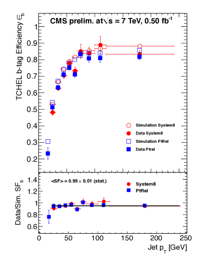
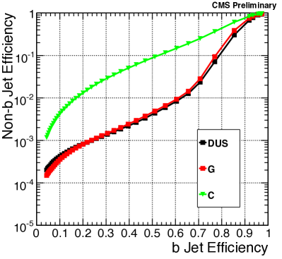
Figure 6.2: Efficiency of tagging a jet originating from the fragmentation of a $b$-quark as a $b$-jet (left) and associated mistagging rates (right). They depend on the transverse momentum of the jet and follow the ‘high efficiency $b$-tagging’ algorithm of CMS (TCHEL). In the upper panel of the left figure (taken from Ref. [528]), the measured and simulated $b$-tagging efficiencies from different methods are presented, while the ratio between data and simulation is shown on its lower panel. In the right panel of the Figure (taken from Ref. [529]), the associated mistagging rates are indicated, as a function of the $b$-tagging efficiency.

The only source of irreducible Standard Model background consists of the production of an invisibly decaying $Z$-boson together with at least three jets, one of them being originated from the fragmentation of a $b$-quark. However, many sources of instrumental background have also to be considered. On the one hand, multijet events with fake missing energy exactly mimic the signal. On the other hand, events originating from the production of a $W$-boson, $t\bar{t}$ pair or a weak boson pair in association with jets contribute as well to the background when the leptons originating from the top quark and weak boson decays are non-reconstructed. Finally, single top events including non-reconstructed or misrecontructed jets must be considered too.

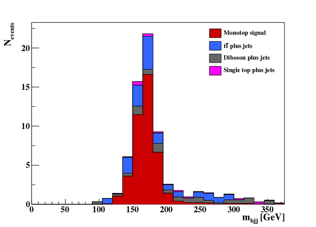
Figure 6.3: After applying the monotop selection strategy presented in the text, we show the invariant-mass distribution of the three jets $m_{bjj}$ both for the signal (red) and the dominant sources of background issued from single top (purple), $t\bar{t}$ (blue) and diboson (gray) processes.

It has been shown, in recent experimental analyses, that a simple selection strategy (as the one performed below) allows to keep a good control over the background [530, 531]. Inspired, in addition, by the parton-level results of Ref. [142], we preselect events containing a large amount of missing transverse energy $\not{E}_{T}>200$ GeV, where

$$\not{E}_{T}=\bigg{|}\bigg{|}\sum_{\text{visible particles}}\vec{p}_{T}\bigg{|}\bigg{|}\ .$$ (6.4.2)

We then impose a veto on the presence of any charged lepton (electron or muon) with a transverse momentum $p_{T}\geq 10$ GeV and a pseudorapidity $|\eta|\leq 2.5$. These selections have been found not to affect the signal but sensibly reduce the contributions of the $t\bar{t}$, $Z$-boson, and $W$-boson events. In a second stage, we exploit the presence of a hadronically decaying top quark and demand exactly one $b$-tagged jet with a transverse momentum $p_{T}\geq 50$ GeV and a pseudorapidity $|\eta|\leq 2.5$, as well as exactly two light jets with a transverse momentum $p_{T}\geq 30$ GeV and a pseudorapidity $|\eta|\leq 2.5$. In our analysis, we estimate a $b$-tagging efficiency depending on the transverse momentum as on Figure 6.2 (left panel), together with a charm and light jet mistagging rate as illustrated on the right panel of the figure. This corresponds to an efficiency of correctly tagging a jet with a transverse momentum of 50 GeV as a $b$-jet of about 70%, whilst the mistagging rate of a charm (light) jet as a $b$-jet is of about 25 % (2%). Since the two selected light jets are issued from the decay of a $W$-boson, we constrain their invariant mass to be compatible with the $W$-mass, i.e., lying in the $65$ GeV$-95$ GeV range.

The distribution of the invariant-mass of the three jets $m_{bjj}$ is presented on Figure 6.3. After applying all the selection criteria described above, the remaining background contributions consists of $t\bar{t}$, diboson and single top events, while all other sources of background, such as $W$-boson or $Z$-boson (or non-simulated multijet) events, are reduced to a(n expected to be) barely visible level and thus not presented in the figure. After further constraining the system of the three selected jets by requiring their invariant-mass to be compatible with the mass of the top quark, lying in a 40 GeV mass window centered around the top mass, we obtain the number of events shown in Table 6.3, both for the signal and the dominant background contributions.

Defining the LHC sensitivity to a monotop signal induced by $R$-parity violating supersymmetry as the number of selected signal events over the total number of selected events $S/\sqrt{S+B}$, the adopted benchmark scenario leads to a possible hint for monotops at the $4.95\sigma$ level. Conversely, a $3\sigma$-deviation from the Standard Model expectation can already be observed for any value of the $R$-parity violating parameter $\hat{\lambda}^{\prime\prime}_{312}\geq 0.11$, assuming the supersymmetric spectrum to be unchanged. Since the number of signal events is not expected to drastically change for moderate superpartner masses (below or around the TeV scale), the standard monotop search strategy presented above is expected to be sufficient to probe $R$-parity violating supersymmetric monotop signatures in large regions of the cMSSM parameter space. This statement will be confirmed in the next chapter.

Event sample	Number of selected events
Top-antitop pair plus jets	$8.2\pm 2.3$
Diboson plus jets	$2.7\pm 0.7$
Single top	$0.9\pm 0.3$
Total background	$11.8\pm 2.4$
Monotop signal	$33.2\pm 1.0$

Table 6.3: Number of selected events after applying the monotop search strategy described in the text for the different background contributions and for the signal. Since approximately no $W$-boson, $Z$-boson and multijet event is passing the selection criteria, these channels are not indicated in the table. These results correspond to 4 fb^-1 of LHC collisions at a center-of-mass energy of 7 TeV.

6.5 Sgluon-induced multitop production in $R$-symmetric supersymmetry

6.5.1 Benchmark scenario and process of interest

We now turn to an investigation of some phenomenology related to sgluon fields dominantly coupling to top quarks as predicted in $R$-symmetric supersymmetric models. Therefore, all superpartners and the numerous Higgs fields are irrelevant, which motivates us to conceive a practical benchmark scenario where all mixing matrices related to the sfermion, neutralino, chargino and Higgs sectors are set to zero so that the related particles do not play any role. In the aim of using the event generator MadGraph 5, the corresponding interaction vertices have been removed from the UFO model files generated by FeynRules by means of the optimization procedure described in Section 6.3.

Our benchmark scenario is defined by fixing the Standard Model inputs, together with the parameters related to the sgluon field, i.e., its mass $M_{\sigma}$ and its couplings to quarks $a_{q}^{L}$, $a_{q}^{R}$ (with $q=u$ and $d$) and gluons $a_{g}$ introduced in Eq. (6.1.15). Although in principle, the sgluon mass $M_{\sigma}$ depends on several soft parameters, i.e., $m_{\tilde{\Phi}_{G}}$, $M_{\tilde{\Phi}_{G}}$ and ${\cal M}_{\tilde{\Phi}_{G}}$ (see Eq. (6.1.9) and Eq. (6.1.13)), and is different for scalar and pseudoscalar sgluons, we simplify the approach by decoupling the pseudoscalar degree of freedom and collecting the three contributions to the scalar mass into a single parameter $M_{\sigma}$. As already mentioned in Section 6.1.2, recent ATLAS and CMS analyses have constrained the sgluon mass to be larger than 2 TeV [510, 511, 512, 513]. These limits however only hold when the sgluon field couple to light quarks and gluons with ${\cal O}(1)$ interaction strengths, and we therefore evade this bound by setting all effective parameters to zero, with the exception of $(a_{u}^{L})^{3}{}_{3}=(a_{u}^{R})^{3}{}_{3}=3\times 10^{-3}$ and $a_{g}=1.5\times 10^{-6}$ GeV^-1. These numbers are obtained by making use of the explicit calculations of the relevant loop diagrams in Ref. [441], and correspond to a benchmark scenario where squarks and gluinos have typical masses of about $1-2$ TeV and where non-minimal flavor violation in the squark sector is not allowed. Lower sgluon masses are thus viable and we set $M_{\sigma}=500$ GeV. The chosen numerical values for the model parameters are summarized in Table 6.4, which also includes the relevant Standard Model inputs taken from the 2010 Review of the Particle Data Group [520].

$M_{t}$ [GeV]	$M_{Z}$ [GeV]	$\alpha_{s}(M_{Z})$	$M_{\sigma}$ [GeV]	$(a_{u}^{L})^{3}{}_{3}$	$(a_{u}^{R})^{3}{}_{3}$	$a_{g}$ [GeV-1]
173.1	91.1876	0.1176	500	$3\times 10^{-3}$	$3\times 10^{-3}$	$1.5\times 10^{-6}$

Table 6.4: Input parameters associated with the chosen benchmark scenario for the $R$-symmetric supersymmetric exploration performed in this work. We recall that the superpartners are decoupled and irrelevant, and that all the omitted effective couplings are taken vanishing.

In this scenario, the total sgluon-pair production cross section, as calculated by MadGraph 5 [64] after convoluting the hard scattering matrix-elements related to the Feynman diagrams of Figure 6.4 with the CTEQ6L1 set of parton densities [522], reach the level of 0.20 pb. Including sgluon decays to a pair of top quarks, sgluon-induced four-top production occurs with a rate of about 42 fb, i.e., more than 140 times the (leading-order) Standard Model predictions of 0.3 fb. Whereas the value of the effective sgluon-gluon-gluon coupling of $1.5\times 10^{-6}$ GeV^-1 may seem very small, the related diagrams contribute to the sgluon-pair production cross section up to about 15%.

Figure 6.4: Tree-level Feynman diagrams associated with sgluon pair production at hadron colliders. These diagrams correspond to the interactions included in the Lagrangians of Eq. (6.1.14) and Eq. (6.1.15) and have been generated by means of the program FeynArts [165].

6.5.2 Phenomenological investigations at 7 TeV

Four-top production leads to final states enriched in jets and leptons that originate from the top decays. Therefore, the main sources of Standard Model background is expected to be related to rare processes with a high final state multiplicity, such as the production of a top-antitop pair in association with one or several gauge bosons or with jets. We generate both signal and background events by employing the same setup as in Section 6.4.2 and refer to this section for more information.

We preselect events containing exactly two charged leptons with a transverse momentum $p_{T}\geq 20$ GeV and a pseudorapidity $|\eta|\leq 2.5$. In addition, we impose them to be isolated so that electrons and muons at a relative distance $\Delta R=\sqrt{\Delta\varphi^{2}+\Delta\eta^{2}}\leq 0.2$ from a jet are rejected, $\varphi$ standing for the azimuthal angle with respect to the beam direction. To ensure a good rejection of the background, dominated by $t\bar{t}$ and Drell-Yan events, and to maintain at the same time a important signal efficiency (of about 50% in our case), we require that the two leptons carry the same electric charge. Moreover, leptonic top decays always imply missing transverse energy $\not{E}_{T}$, so that we only keep events with $\not{E}_{T}\geq 40$ GeV.

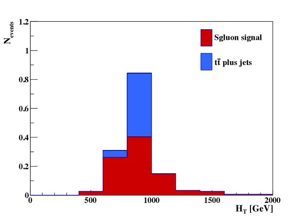
Figure 6.5: After applying the sgluon search strategy in the dilepton channel presented in the text, we present the distribution of the $H_{T}$ variable defined in Eq. (6.5.1) for both the signal (red) and the dominant source of background consisting of $t\bar{t}$ events (blue).

The rest of the proposed sgluon search strategy benefits from the important jet multiplicity specific to signal events. In particular, we expect at least four $b$-tagged jets (one for each of the produced top quarks) and four additional light jets originating from the hadronically decaying top quarks. Consequently, we demand the selected events to contain at least eight jets with a transverse energy $E_{T}\geq 20$ GeV, and impose that at least three of them are $b$-tagged, the $b$-tagging efficiency and the corresponding mistagging rates being defined as in Section 6.4.2. The important hadronic activity in the final state suggests to employ the $H_{T}$ variable, defined by

$$H_{T}=\sum_{\text{jets, leptons, missing energy}}\big{|}\big{|}\vec{p}_{T}\big{|}\big{|}\ ,$$ (6.5.1)

as a discriminating variable between signal and backgrounds. The results are presented in Figure 6.5 and in Table 6.5. The dominant contributions to the background consist in $t\bar{t}$ events, as well as, in a smaller extent (and therefore not shown), in events issued from the production and decay of a $t\bar{t}$ pair accompanied by one or several gauge bosons. Although the background rejection is efficient, a 4 fb^-1 luminosity of 7 TeV collisions is unfortunately not sufficient to obtain a good sensitivity to the sgluon signal, at least for a 500 GeV sgluon mass. This naive analysis has therefore to be improved, a task addressed in the next chapter.

Two remarks are in order here. First, our event selection criteria may seem very restrictive, in particular concerning the number of required jets and $b$-tags. However, these selections are mandatory to ensure a good background rejection, as shown in Ref. [77] where the effects or requiring different numbers of jets and $b$-tags have been investigated. Next, in our simulation setup, the multijet background, jets faking leptons and charge misidentification have not been accounted for. On the basis of the analysis of Ref. [532] where same sign dilepton events are investigated after selection criteria similar to those applied in this analysis, these sources of background have been found to be dominant. This issue is addressed more into details in Chapter 7, as this does not change the conclusions of the 7 TeV analysis of this section.

Event sample	Number of selected events
Top-antitop pair plus jets	$0.5\pm 0.3$
Total background	$0.5\pm 0.3$
Sgluon signal	$0.9\pm 0.1$

Table 6.5: Number of selected events after applying the dilepton sgluon search strategy presented in the text for the different background contributions and for the signal. Since approximately no event related to all the other sources of background is passing the selection criteria, these channels are not indicated in the table. The results correspond to an integrated luminosity of 4 fb^-1 of proton-proton collisions at the LHC collider, running with a center-of-mass energy of 7 TeV.

Chapter 7 From non-minimal supersymmetry to effective field theories

The search, in particular at the LHC, of tracks of new phenomena moves in several directions. The most beaten path, as illustrated in Chapter 6, lies on a top-down approach. In this case, a theory extending the Standard Model of particle physics is conceived on the basis of fundamental theoretical principles, such as an extended symmetry group or additional spacetime dimensions. This theory is constructed in a way to reproduce the Standard Model in the low energy limit and to possibly address one or more of the Standard Model open issues, such as the hierarchy problem like in supersymmetry (see Section 5.2.1). Predictions of physical observables can then be made by making use of perturbation theory. However, many new parameters, that cannot be fixed by experimental constraints, usually enter the calculations. For the sake of the examples, we recall the large size of the parameter space of the models presented in Chapter 5 and in Chapter 6, these models featuring up to several hundreds of free parameters in their general form. Benchmark scenarios must therefore be carefully designed in order to be compatible with (most of) current data and they subsequently imply typical signatures for the model that can be searched for in present and future experiments, such as the missing energy requirement in supersymmetry.

While widely used, this theory-driven approach has notable limitations. First, signatures are neither typical of a given benchmark nor of a specific model itself. For instance, universal extra dimensions and supersymmetry can have very similar signatures involving cascade decays of heavy particles. Next, the top-down approach can lead to strong biases in the experimental analyses. Therefore, it is important to pursue a more pragmatic approach where beyond the Standard Model explorations based on a bottom-up construction of new physics models are supplemented to the more common top-down inspired analyses.

In the following, we employ the tool of effective low energy theories to explore different scenarios built from the two experimental signatures investigated in Section 6.4.2 and Section 6.5.2. We analyze in this way several classes of models simultaneously for monotop searches (Section 7.1.1 and Section 7.3) and sgluon-induced multitop final states (Section 7.1.2 and Section 7.4). Additionally, we detail in Section 7.2 our simulation setup for the Standard Model background.

7.1 Effective theories inspired by non-minimal supersymmetry

7.1.1 An effective field theory for monotop production

Figure 7.1: Representative Feynman diagrams leading to a monotop signature, either through the resonant exchange of a colored scalar field $S$ (left) or via a flavor-changing interaction with a vector field $V$ (right). The $V$ and $\chi$ particles are here invisible and lead to missing energy.

Beyond supersymmetry and at tree-level, monotop production can occur via two main mechanisms. Either the top quark is produced, possibly resonantly, in association with an invisible fermionic state (see, e.g., the representative Feynman diagram shown on the left panel of Figure 7.1) or through a flavor-changing interaction with an invisible bosonic state (see, e.g., the representative Feynman diagram shown on the right panel of Figure 7.1).

Within the first production mechanism, the top quark is produced together with an undetected fermion which we denote, in the following, by $\chi$. Possible diagrams occur via $s$-channel (see Figure 7.1), $t$-channel and $u$-channel exchanges of a scalar ($S$) or vector ($V$) field lying in the (anti-)fundamental representation of $SU(3)_{c}$. As shown in Section 6.4, such processes appear in $R$-parity-violating supersymmetry where, similarly to the case discussed in Ref. [533], the intermediate particle is a (possibly on-shell) top squark and $\chi$ consists of the lightest neutralino,

$$\bar{d}\bar{s}\to\tilde{t}_{i}\to t\tilde{\chi}_{1}^{0}\ .$$ (7.1.1)

In the limit of very heavy resonances, monotops can also be seen as produced through a baryon number-violating four-fermion effective interaction [534, 535]. More exotic cases can involve invisible Rarita-Schwinger fields, as in supersymmetric theories containing a spin-$3/2$ gravitino field, or a multiparticle state with a global half-integer spin, as in hylogenesis scenarios for dark matter [536].

In the second class of models yielding a monotop signature, the missing energy is carried by a neutral bosonic state, either long-lived or decaying invisibly. Monotops are arising from quark-gluon initial states undergoing a flavor-changing interaction, as discussed, e.g., in Ref. [537]. In this case, the missing energy can be either a spin-zero $S$, spin-one $V$ (see Figure 7.1) or spin-two $G$ state,

$$ug\to tS\ ,\quad ug\to tV\quad\text{ or }\quad ug\to tG\ ,$$ (7.1.2)

or can also be a continuous state containing an even number of fermions, as in $R$-parity conserving supersymmetry with non-minimal flavor violation (see Section 5.3) [538],

$$ug\to\tilde{u}_{i}\tilde{\chi}_{1}^{0}\to t\tilde{\chi}_{1}^{0}\tilde{\chi}_{1}^{0}\ .$$ (7.1.3)

The properties of the produced top quark are induced by the features of the production mechanism. First, the partonic content of the initial state and the nature (mass and spin) of the undetected recoiling object play a key role. Next, the possible presence of intermediate resonant states could alter kinematical distributions such as the transverse-momentum spectrum of the final state particles. Following the spirit of Ref. [539], these considerations suggest a model-independent approach including all the cases within a single simplified theory. Assuming the strong interactions to be flavor-conserving, as in the Standard Model, the flavor-changing neutral interactions are bound to the weak sector. For simplicity, we also neglect spin-two gravitons, since their flavor-changing interactions are loop-suppressed [540], as well as any of their excitations which do not lead to a missing energy signature. Along the same lines, we do not consider spin-$3/2$ fields since their (flavor-violating or not) couplings are, at least in supersymmetric theories, suppressed by a high-energy scale. In addition, four-fermion interactions are omitted as they are known not to lead to a visible LHC signal [142].

In our construction of an effective Lagrangian for monotop production, we denote by $\phi$, $\chi$ and $V$ the possible scalar, fermionic and vector particle leading to missing energy, respectively, and by $\varphi$ and $X$ scalar and vector fields lying in the fundamental representation of $SU(3)_{c}$ possibly inducing resonant monotop production. The Lagrangian describing the interactions of those fields is supplemented to the Standard Model Lagrangian and reads, in the mass basis,

$$\begin{split}{\cal L}&=\ {\cal L}_{\rm kin}+\bigg{[}\phi\bar{u}\Big{[}a^{0}_{FC}\!+\!b^{0}_{FC}\gamma_{5}\Big{]}u\!+\!V_{\mu}\bar{u}\Big{[}a^{1}_{FC}\gamma^{\mu}\!+\!b^{1}_{FC}\gamma^{\mu}\gamma_{5}\Big{]}u\\ &+\!\epsilon^{ijk}\varphi_{i}\bar{d}^{c}_{j}\Big{[}a^{q}_{SR}\!+\!b^{q}_{SR}\gamma_{5}\Big{]}d_{k}\!+\!\varphi_{i}\bar{u}^{i}\Big{[}a^{1/2}_{SR}\!+\!b^{1/2}_{SR}\gamma_{5}\Big{]}\chi\\ &+\epsilon^{ijk}X_{\mu,i}\ \bar{d}^{c}_{j}\Big{[}a^{q}_{VR}\gamma^{\mu}+b^{q}_{VR}\gamma^{\mu}\gamma_{5}\Big{]}d_{k}+X_{\mu,i}\ \bar{u}^{i}\Big{[}a^{1/2}_{VR}\gamma^{\mu}+b^{1/2}_{VR}\gamma^{\mu}\gamma_{5}\Big{]}\chi+{\rm h.c.}\bigg{]}\ ,\end{split}$$ (7.1.4)

where kinetic and gauge interaction terms for the new states are included in ${\cal L}_{\rm kin}$ and where the indices $i$, $j$ and $k$ represent color indices in the fundamental representation of $SU(3)_{c}$. Additionally, flavor indices have been understood. The $3\times 3$ matrices (in flavor space) $a^{\{0,1\}}_{FC}$ and $b^{\{0,1\}}_{FC}$ contain quark interactions with the bosonic invisible particles $\phi$ and $V$, while $a^{1/2}_{\{S,V\}R}$ and $b^{1/2}_{\{S,V\}R}$ denote the couplings between up-type quarks, the invisible fermion $\chi$ and the new colored states $\varphi$ and $X$. Moreover, gauge invariance also allows the latter to couple to down-type quarks, the corresponding interaction strengths being given by the matrices $a^{q}_{\{S,V\}R}$ and $b^{q}_{\{S,V\}R}$.

To illustrate the main features of monotop production, we consider a series of simplified scenarios in which all axial couplings involving new particles vanish,

$$b=0\ .$$ (7.1.5)

Furthermore, we only retain interactions that can be enhanced by parton densities and set

$$\begin{split}(a^{0}_{FC})_{13}=(a^{0}_{FC})_{31}=(a^{1}_{FC})_{13}=(a^{1}_{FC})_{31}=a\ ,\\ (a^{q}_{SR})_{12}=\ -(a^{q}_{SR})_{21}=(a^{1/2}_{SR})_{3}=(a^{q}_{VR})_{11}=(a^{1/2}_{VR})_{3}=a\ ,\end{split}$$ (7.1.6)

the other couplings being fixed to zero. Within the above settings, we define four scenarios, the first two, which we denote by S.I and S.II, addressing resonant monotop production and the last two, which we denote by S.III and S.IV, focusing on monotop production via baryon-number conserving but flavor-changing interactions. We now turn to the evaluation of monotop production cross section at the LHC, running at a center-of-mass energy of 8 TeV and employ the QCD factorization theorem to convolute the associated leading order squared matrix elements with the leading order set of the CTEQ6 parton density fit [522], fixing both the renormalization and factorization scales to the transverse mass of the monotop system. To this aim, we implement the Lagrangian above into FeynRules, and export the model into a UFO library which is then linked to MadGraph 5.

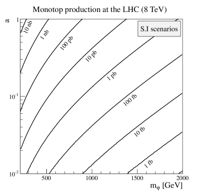
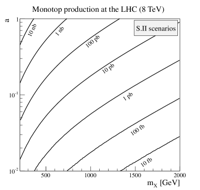
Figure 7.2: Total cross sections for monotop production at the LHC, running at a center-of-mass energy of 8 TeV, for scenarios of type S.I (left panel) and S.II (right panel) respectively featuring a scalar and vector colored resonance decaying with a branching fraction of one into a monotop state. The cross sections are presented as a function of the new physics coupling $a$ and of the resonance mass $m_{\varphi}$ (scalar resonance) and $m_{X}$ (vector resonance).

In scenarios of type S.I and S.II, we also assume that the new colored scalar $\varphi$ and vector $X$ resonances decay into a top quark and an invisible particle $\chi$ with a branching ratio equal to one. Consequently, this renders our analysis insensitive to the parameters $(a^{q}_{SR})_{3}$ and $(a^{q}_{VR})_{3}$ and the S.I and S.II scenarios are described by only three parameters, namely the couplings of the down-type quarks to the new resonance $a$, the resonance mass $m_{\varphi}$ (for scenarios of class S.I) and $m_{X}$ (for scenarios of class S.II) and the mass of the invisible particle $m_{\chi}$. Monotop production cross sections are however independent of the invisible particle mass as they are equal to the colored new particle production cross section, the subsequent branching ratio into a $t\chi$ pair being unity. The mass difference between the resonance and the missing energy particle however alters the selection efficiency of any monotop search strategy as it modifies the available phase space for the decay (see Section 7.3 for more details). The dependence of the monotop production cross section on the resonance mass and on the new physics coupling strength $a$ is illustrated on Figure 7.2 for scenarios involving a scalar resonance S.I (left panel of the figure) and a vector resonance S.II (right panel of the figure). Cross sections reaching the pb level are expected for a moderate coupling strength of $a=0.1$ and resonance masses around (in the scalar case) or even above (in the vector case) 1 TeV. For given resonance mass and coupling strength, it is also found that a monotop signature induced by a vector state is produced with a larger rate as when arising from the decay of a scalar state due to the different Lorentz structure of the interactions of the Lagrangian of Eq. (7.1.4) and to the larger number of propagating degrees of freedom of a vector field.

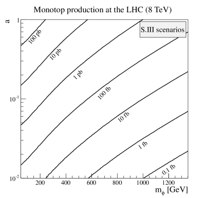
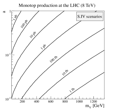
Figure 7.3: Total cross sections for monotop production at the LHC, running at a center-of-mass energy of 8 TeV, for scenarios of type S.III (left panel) and S.IV (right panel) respectively featuring a flavor-changing production of a top quark in association with a scalar and vector invisible state. The cross sections are presented as a function of the new physics coupling $a$ and of the invisible particle mass $m_{\phi}$ (scalar case) and $m_{V}$ (vector case).

In scenarios of class S.III and S.IV, the top quark is produced in association with a bosonic particle through a flavor-changing interaction in the weak sector. The bosonic state, being respectively a scalar and vector particle in the two scenarios, is further non-detected and gives rise to missing energy. The S.III and S.IV scenarios are thus described by exactly two parameters, the mass of the missing energy particle $m_{\phi}$ and $m_{V}$ in the scalar and vector cases, respectively, and the strength of the flavor-changing interaction of this particle with a pair of quarks comprised of one top quark and one up quark. Cross sections for monotop production in the flavor-changing mode are presented as a function of these two parameters in Figure 7.3 for a scalar (left panel of the figure) and vector (right panel of the figure) invisible state. In contrast to the first two scenarios where TeV-scale new physics can be associated with a cross section of 1 pb for a moderate coupling strength of $a=0.1$, such a cross section value corresponds to much lighter invisible particle masses of about 300 GeV and 500 GeV for scenarios of type S.III and S.IV, respectively, and an identical coupling value of $a=0.1$. Once again, larger cross sections are associated with the vector case due to the more important number of polarization states and the Lorentz structures of the possible interactions.

7.1.2 A simplified model for sgluon production and decays at the LHC

In Section 6.5.2, we have illustrated a phenomenological aspect of sgluon fields in the framework of the minimal version of $R$-symmetric supersymmetric theories [139, 140, 141], considering their contributions to the production rate of multitop final states. However, sgluon fields are also predicted in other models, such as in $N\!=\!1\!/\!N\!=\!2$ hybrid supersymmetric theories [439, 440, 441, 442, 443, 444, 445, 446, 447], in vector-like confining theories [541, 542, 543, 544, 545, 546] or in extra-dimensional models [547].

All these new physics models contain a sgluon sector with similar properties as in $R$-symmetric supersymmetry. This motivates us to construct a simplified effective model describing a scalar field lying in the octet representation of the QCD gauge group and its interactions with the Standard Model sector [143, 548]. This leaves open the possibility of reinterpreting the results in the context of any of the original models, or even in the framework of any other theory including a sgluon field. In addition, it avoids the careful design of a theoretically motivated and not experimentally excluded benchmark scenario for the complete model, the simplified model being instead described by a small number of couplings and masses.

We extend the Standard Model in a minimal way by supplementing to its particle content one real scalar field $\sigma$ of mass $M_{\sigma}$ lying in the adjoint representation of the QCD gauge group. Its kinetic, mass and gauge interaction terms are standard,

$${\cal L}_{\rm kin}=\frac{1}{2}D_{\mu}\sigma^{a}D^{\mu}\sigma_{a}-\frac{1}{2}M_{\sigma}^{2}\sigma^{a}\sigma_{a}\ ,$$ (7.1.7)

and are expressed in terms of the QCD covariant derivative taken in the adjoint representation

$$D_{\mu}\sigma^{a}=\partial_{\mu}\sigma^{a}+g_{s}\ f_{bc}{}^{a}\ g_{\mu}^{b}\ \sigma^{c}\ ,$$ (7.1.8)

for which we recall that the strong coupling constant is denoted by $g_{s}$, the antisymmetric structure constants of $SU(3)_{c}$ by $f_{bc}{}^{a}$ and that the gluon field reads $g_{\mu}$.

In Eq. (6.1.15), we have introduced, in the context of minimal $R$-symmetric supersymmetry, loop-induced interactions of a single sgluon to the Standard Model partons. This feature also holds in other theories, where the presence of additional particles in general implies loop diagrams yielding dimension-four and dimension-five effective operators involving up-type quarks $u$, down-type quarks $d$ and gluons,

$${\cal L}_{\rm eff}=\sigma^{a}\bar{d}T_{a}\Big{[}a^{L}_{d}P_{L}+a^{R}_{d}P_{R}\Big{]}d+\sigma^{a}\bar{u}T_{a}\Big{[}a^{L}_{u}P_{L}+a^{R}_{u}P_{R}\Big{]}u+a_{g}d_{a}{}^{bc}\sigma^{a}G_{\mu\nu b}G^{\mu\nu}{}_{c}+{\rm h.c.}\ ,$$ (7.1.9)

referring to Eq. (6.1.15) for the notations. These interactions consequently open all possible sgluon decays into Standard Model colored particles. Inspecting the two Lagrangians of Eq. (7.1.7) and Eq. (7.1.9), our simplified theory is described by one mass parameter, the sgluon mass $M_{\sigma}$, and the effective couplings of sgluons to colored partons described by a set of four complex $3\times 3$ matrices in flavor space $a^{L}_{d}$, $a^{R}_{d}$, $a^{L}_{u}$ and $a^{R}_{u}$ and one real dimensionful number $a_{g}$.

As already mentioned in Section 6.5.1, sgluon masses up to about 2 TeV are excluded by dijet resonance searches [511] once we assume ${\cal O}(1)$ effective sgluon interactions to light quarks. We therefore focus, motivated by $R$-symmetric supersymmetry, on scenarios where the sgluon field dominantly decays into final states containing at least one top quark and where its couplings to a pair of light quarks or to a pair of gluons are reduced so that the experimental constraints can be evaded. This brings us to consider two series of benchmark scenarios.

Parameters	Scenarios of type S.I	Scenarios of type S.II
$a_{g}$	$1.5\times 10^{-6}$ GeV-1	$1.5\times 10^{-6}$ GeV-1
$(a_{u})^{3}{}_{3}$	$3\times 10^{-3}$	$3\times 10^{-3}$
$(a_{u})^{3}{}_{1}=(a_{u})^{1}{}_{3}$	$3\times 10^{-3}$	0
$(a_{u})^{3}{}_{2}=(a_{u})^{2}{}_{3}$	$3\times 10^{-3}$	0
$M_{\sigma}$	[200-1000] GeV	[400-1000] GeV
$M_{t}$	172 GeV	172 GeV

Table 7.1: Non-zero input parameters for benchmark scenarios of class S.I and S.II. For all the other Standard Model parameters, we follow the conventions of Ref. [74].

For the first set of scenarios, referred to as scenarios of class S.I, sgluon particles are allowed to decay in a universal way to any associated pair of up-type quarks containing at least one top quark, so that

$$(a^{L}_{u})^{3}{}_{i}=(a^{R}_{u})^{3}{}_{i}=(a^{L}_{u})^{i}{}_{3}=(a^{R}_{u})^{i}{}_{3}=3\times 10^{-3}\ ,$$ (7.1.10)

for $i=1,2,3$. We subsequently impose that any other interaction among quarks and a single sgluon vanishes. Concerning the parameter $a_{g}$, we choose the value

$$a_{g}=1.5\times 10^{-6}\text{ GeV}^{-1}\ .$$ (7.1.11)

Both Eq. (7.1.10) and Eq. (7.1.11) correspond to a supersymmetry mass scale of about 2 TeV (as shown by the analytical formulas presented in Ref. [441]), in agreement with the current experimental results related to direct searches for squarks and gluinos at the LHC (see Section 5.5).

In our second class of scenarios, denoted as scenarios of class S.II, we focus exclusively on sgluon-induced signatures with four top quarks so that the only states into which a sgluon decays consist of either a top-antitop or a gluon pair, the only non-vanishing effective interactions being thus driven by the coupling parameters

$$(a^{L}_{u})^{3}{}_{3}=(a^{R}_{u})^{3}{}_{3}=3\times 10^{-3}\qquad\text{and}\qquad a_{g}=1.5\times 10^{-6}\text{ GeV}^{-1}\ .$$ (7.1.12)

In addition, we fix for both classes of scenarios the mass of the top quark to $M_{t}=172$ GeV, all the other Standard Model parameters according to the conventions of Ref. [74] and allow the sgluon mass $M_{\sigma}$ to vary below 1 TeV. We summarize in Table 7.1 the values of all non-zero parameters of the Lagrangians of Eq. (6.1.14) and Eq. (6.1.15).

Scenario	$M_{\sigma}$ [MeV]	$\Gamma_{\sigma}$ [GeV]	BR$[t\bar{t}]$	BR$[tj/\bar{t}j]$	BR$[gg]$	$\sigma_{\rm tot}$ [fb]	$K_{\rm NLO}$
S.I	200	0.012	-	80%	20%	98600	1.6
S.I	300	0.105	-	92.3%	7.7%	9802	1.6
S.I	400	0.219	4.4 %	86.9%	8.7%	1625	1.7
S.II		0.029	33.3%	-	66.7%
S.I	500	0.35	9.8 %	79.5%	10.1%	358.1	1.8
S.II		0.072	47.8%	-	52.2%
S.I	600	0.485	12 %	75%	13%	94.9	1.8
S.II		0.124	48%	-	52%
S.I	700	0.628	13.2 %	70.5%	16.3%	28.4	1.9
S.II		0.185	44.7%	-	55.3%
S.I	800	0.779	13.5 %	66.9%	19.6%	9.26	2.0
S.II		0.252	41%	-	59%
S.I	900	0.943	13.5 %	63.4%	23.1%	3.22	2.1
S.II		0.345	36.9%	-	63.1%
S.I	1000	1.12	13.2 %	60.2%	26.6%	1.17	2.2
S.II		0.447	33.2%	-	66.8%

Table 7.2: Dependence on the sgluon mass $M_{\sigma}$ of the sgluon total width ($\Gamma_{\sigma}$), of its branching fractions to a top-antitop pair (BR$[t\bar{t}]$), to an associated pair of a top (anti)quark and a light quark (BR$[tj/\bar{t}j]$) and to a gluon pair (BR$[gg]$), as well as of its total pair-production cross section at leading order and at the LHC collider running at a center-of-mass energy of 8 TeV ($\sigma_{\rm tot}$). The next-to-leading order $K$-factors ($K_{\rm NLO}$) are also indicated.

A key element in the multitop analysis of sgluon production and decay at the LHC lies in the sgluon branching fraction to final states containing one or two top quarks. We investigate the evolution of these branching ratios with the sgluon mass by implementing the Lagrangians of Eq. (6.1.14) and Eq. (6.1.15) into FeynRules, following the syntax introduced in Chapter 3, and by subsequently exporting the model to the UFO format so that it can be used within the MadGraph 5 framework. This matrix-element generator is then employed to estimate the total sgluon width and the different branching ratios into two gluons, an associated pair of a top quark and a light quark and into two top quarks. The results are shown in Table 7.2 for both classes of scenarios.

The branching of a light sgluon of a couple of hundreds of GeV into a $t\bar{t}$ pair is kinematically suppressed compared to the other open decay channels for both types of scenarios. This branching ratio then increases with the sgluon mass, although the contributions of the dijet ($\sigma\to gg$) channel to the total width also become more important. Therefore, the branching into a top-antitop pair peaks for $M_{\sigma}\sim 800$ GeV and $M_{\sigma}\sim 600$ GeV for scenarios of type S.I and S.II, respectively, and then decreases for heavier sgluons.

Table 7.2 also contains the leading-order sgluon pair-production cross sections as computed with the MadGraph 5 program. The numerical values are calculated in the context of the LHC collider running at a center-of-mass energy of 8 TeV and after convoluting the matrix elements related to the Feynman diagrams of Figure 6.4 with the leading order set of the CTEQ6 parton density fit [522], fixing both the renormalization and factorization scales to the transverse mass of the sgluon pair. Next-to-leading order corrections to those cross sections have been recently computed within the MadGolem setup [549, 550], and the corresponding $K$-factors are presented in the last column of the table.

7.2 Monte Carlo simulations of the Standard Model background

7.2.1 Simulation setup

Process	$k_{T}^{\rm min}$ [GeV]	$p_{T}^{\rm min}$ [GeV]	$n$	$Q^{\rm m}$ [GeV]	$\sigma$ [pb]	$N$
$W(\to\ell\nu)+\text{jets}$	10	10	4	20	35678	$2.56\cdot 10^{8}$
$\gamma^{*}/Z(\to 2\ell/2\nu)+\text{jets}$	10	10	4	20	10319	$4\cdot 10^{7}$
$t\bar{t}(\to 6\text{jets})\!+\!\text{jets}$	20	20	2	30	116.2	$8\cdot 10^{6}$
$t\bar{t}(\to 4\text{jets}\ 1\ell\ 1\nu)\!+\!\text{jets}$	20	20	2	30	112.4	$9\cdot 10^{6}$
$t\bar{t}(\to 2\text{jets}\ 2\ell\ 2\nu)\!+\!\text{jets}$	20	20	2	30	27.2	$3\cdot 10^{6}$
$t/\bar{t}+\text{jets}$ [$t$, incl.]	-	-	0	-	87.2	$6\cdot 10^{6}$
$t/\bar{t}+\text{jets}$ [$tW$, incl.]	-	-	0	-	22.2	$1\cdot 10^{6}$
$t/\bar{t}+\text{jets}$ [$s$, incl.]	-	-	0	-	5.55	$8\cdot 10^{5}$
$WW(\to 1\ell\ 1\nu\ 2\text{jets})\!+\!\text{jets}$	10	10	2	20	24.3	$3\cdot 10^{6}$
$WW(\to 2\ell\ 2\nu)+\text{jets}$	10	10	2	20	5.87	$8\cdot 10^{5}$
$WZ(\to 1\ell\ 1\nu\ 2\text{jets})+\text{jets}$	10	10	2	20	5.03	$5\cdot 10^{5}$
$WZ(\to 2\nu\ 2\text{jets})+\text{jets}$	10	10	2	20	2.98	$3\cdot 10^{5}$
$WZ(\to 2\ell\ 2\text{jets})+\text{jets}$	10	10	2	20	1.58	$2\cdot 10^{5}$
$WZ(\to 1\ell\ 3\nu)+\text{jets}$	10	10	2	20	1.44	$2\cdot 10^{5}$
$WZ(\to 3\ell\ 1\nu)+\text{jets}$	10	10	2	20	0.76	$2\cdot 10^{6}$
$ZZ(\to 2\nu\ 2\text{jets})+\text{jets}$	10	10	2	20	2.21	$3\cdot 10^{5}$
$ZZ(\to 2\ell\ 2\text{jets})+\text{jets}$	10	10	2	20	1.18	$1.5\cdot 10^{4}$
$ZZ(\to 4\nu)+\text{jets}$	10	10	2	20	0.63	$1\cdot 10^{5}$
$ZZ(\to 2\nu\ 2\ell)+\text{jets}$	10	10	2	20	0.32	$4\cdot 10^{4}$
$ZZ(\to 4\ell)+\text{jets}$	10	10	2	20	0.17	$4\cdot 10^{4}$
$t\bar{t}W+\text{jets}$ [incl.]	10	10	2	20	0.25	$3\cdot 10^{4}$
$t\bar{t}Z+\text{jets}$ [incl.]	10	10	2	20	0.21	$5\cdot 10^{4}$
$t/\bar{t}+Z+j+\text{jets}$ [incl.]	6.5	20	1	10	0.046	$3\cdot 10^{5}$
$t\bar{t}WW+\text{jets}$ [incl.]	10	10	2	20	0.013	$2\cdot 10^{3}$
$t\bar{t}t\bar{t}+\text{jets}$ [incl.]	-	-	0	-	$7\cdot 10^{-4}$	$10^{3}$

Table 7.3: Simulated background processes given together with the applied parton-level selection criteria ($k_{T}^{\rm min}$ and $p_{T}^{\rm min}$), the number of allowed extra hard emissions at the matrix-element level ($n$) and the merging scale ($Q^{\rm m}$). The numerical values employed for the cross sections ($\sigma$) are also shown, together with the number of generated events ($N$). We detail each of the background contributions according to the final state signature, $\ell$ standing equivalently for electrons, muons, leptonic and hadronic taus, $\nu$ for any neutrino, and jets or $j$ for any kind of jet. Moreover, the notation incl. indicates that the produced samples are inclusive in the decays of the produced particles. We refer to the rest of this section for more information, in particular on the adopted values for the cross sections.

This chapter aims to estimate the LHC sensitivity to the presence of monotops and sgluons-induced multitop events by means of Monte Carlo simulations. We consider the LHC collider running at a center-of-mass energy of $\sqrt{s}=8$ TeV and normalize our event samples to an integrated luminosity of 20 fb^-1. The hard scattering processes related to the different sources of background are described with the matrix-element generator MadGraph 5. Using the QCD factorization theorem, the matrix elements are convoluted with the leading order set of the CTEQ6 parton density fit [522], the renormalization and factorization scales being fixed to the transverse mass of the produced heavy particles and all quark masses but the top mass are neglected. Parton-level events are integrated into a full hadronic environment by matching the hard scattering matrix elements with a parton showering and hadronization infrastructure as provided by the Pythia 6 package [45]. Moreover, since the generated parton-level events are allowed to contain tau leptons, we make use of the Tauola program [551] to handle their decays.

Typical final states to be produced at the LHC contain in general abundant initial state QCD radiation that has important effects on the shapes of the kinematical distributions. In particular, large logarithmic contributions arise in phase space regions where these additional partons are neither widely separated nor hard. As a consequence, reliable theoretical predictions require a consistent reorganization of the logarithmic terms which have to be resummed to all orders in the strong coupling, embedded in this way within the so-called Sudakov form factor.

In phenomenological investigations relying on Monte Carlo simulations, additional jet production is traditionally simulated using parton showering programs. These tools describe QCD emissions as successive branchings of a mother parton into two daughter partons, the associated probability laws being based on Markov chain techniques built upon the Sudakov form factor. The latter must however be approximated in a way allowing for a description in terms of a Monte Carlo algorithm, which enforces to truncate it, in general, to the leading logarithmic accuracy. This description is formally only correct in the phase space regions where QCD radiation is soft and collinear and fails when considering the production of hard and widely separated additional partons. In this case, matrix elements describing the same final state together with an additional parton are required.

In order to obtain a good description over the whole kinematical range, parton showering and matrix element methods have to be eventually matched. We then allow for the matrix elements to contain up to $n$ additional hard jets and merge the $n+1$ different samples, after parton showering, following the $k_{T}$-MLM merging scheme [86] as implemented in the MadEvent generator [87] interfaced to Pythia 6 [45]. In this setup, two parton-level selection criteria are imposed. Firstly, parton-level final state jets are generated with a minimum jet measure $k_{T}$ larger than a process-dependent threshold $k_{T}^{\rm min}$. The quantity $k_{T}$ is defined, when considering two final state jets labeled by $i$ and $j$, by

$$k_{T}^{2}=\min(p_{Ti}^{2},p_{Tj}^{2})R_{ij}\ ,$$ (7.2.1)

where $p_{Ti}$ and $p_{Tj}$ are the transverse momenta of the jets and $R_{ij}$ their angular distance in the $(\eta,\varphi)$ plane, $\eta$ denoting the pseudorapidity and $\varphi$ the azimuthal angle with respect to the beam direction. Secondly, in order to ensure better QCD factorization properties with respect to initial-state collinear singularities [552], we define the jet measure related to an initial state splitting as its transverse momentum,

$$k_{T}=p_{Ti}\ ,$$ (7.2.2)

and ask it to be larger than a process-dependent value $p_{T}^{\rm min}$.

The events are then passed to Pythia for parton showering and jets are reconstructed making use of a $k_{T}$-jet algorithm [525] with a (process-dependent) cut-off scale $Q^{\rm m}$. A jet is said to be matched to one of the original partons only if the jet measure between the jet and this parton is smaller than $Q^{\rm m}$. In our procedure, only events where each jet is matched to one parton and where each parton is related to one jet are retained, with the exception of events belonging to the sample with the highest jet multiplicity. In this case, extra jets are allowed, which maintains the full inclusiveness of the merged sample. A correct choice for the merging parameters $k_{T}^{\rm min}$, $p_{T}^{\rm min}$ and $Q^{\rm m}$ is crucial since this allows for a coherent splitting of the phase space among regions dominated by matrix-element-based predictions and regions where parton showering correctly describes QCD emission.

In order to probe the smoothness of the transition between these regions, differential jet rate spectra are traditionally investigated. This class of variables consists of the distributions of the scale at which a specific event switches from a $N$-jet configuration to a $N+1$-jet configuration, for various values of the integer number $N$. The merging procedure has been validated for all simulated background contributions. For brevity, we only illustrate this validation in the context of $Z$-boson production (see Section 7.2.2).

The values chosen for the parton-level selection thresholds $p_{T}^{\rm min}$ and $k_{T}^{\rm min}$, the maximum number of included hard emissions $n$ and the merging scale $Q^{\rm m}$ are indicated in Table 7.3 for the various background processes that have been simulated. This table also contains the cross section values $\sigma$ employed for the normalization of the different samples and the numbers of generated events $N$.

7.2.2 Single boson production in association with jets

In terms of cross section, the main contributions to the Standard Model background originate from single weak gauge boson production in association with jets. After imposing the gauge bosons to decay either leptonically or invisibly,

$$\begin{split}pp\to W+\text{ jets }\to&\ \ \ell\nu+\text{ jets }\ ,\\ pp\to Z+\text{ jets }\to\ell\ell+\text{ jets }\ ,\qquad&pp\to Z+\text{ jets }\to\nu\nu+\text{ jets }\ ,\end{split}$$ (7.2.3)

where $\ell$ and $\nu$ generically denote any charged lepton (including the tau) and neutrino, respectively, we have merged event samples containing up to four additional hard jets. We choose the jet measure thresholds to be $p_{T}^{\rm min}=k_{T}^{\rm min}=10$ GeV and fix the merging scale to $Q^{\rm m}=20$ GeV. The suitability of these parameters is checked on Figure 7.4 where we present differential jet rate distributions for $pp\to Z+0,1,2,3$ and 4 jets events, the figures having been computed by making use of the MadAnalysis 5 package [85].

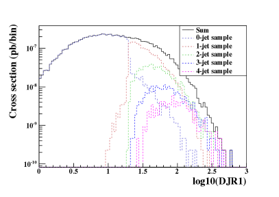
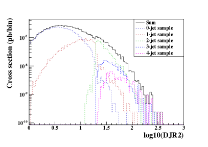
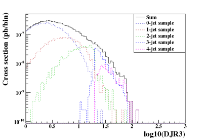
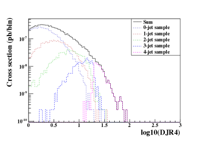
Figure 7.4: Differential jet rate distributions for the process $pp\to Z+$ 0, 1, 2, 3, and 4 jets, where multiparton matrix elements have been merged by employing the $k_{T}$-MLM scheme.

On the left panel of the upper line of the figure, we show the $1\to 0$ differential jet rate distribution, or in other words, the distribution of the scale at which an event passes from a configuration where no final state jet remains after reconstruction to a configuration with one single final state jet does. It is found that only events related to the production of a $Z$-boson without any extra hard jet contribute to the region to the left of the cut-off scale $Q^{\rm m}$ where parton radiation is dominated by parton showering. All the other events (with one hard jet or more at the matrix-element level) contribute to the region located to the right of the cut-off scale, radiation being here correctly described by means of matrix elements. From the figure, the cut-off scale is extracted and found to be equal to 20 GeV, in agreement with the Monte Carlo setup. Similar analyses can be performed for the $2\to 1$ (right panel of the upper line of the figure), $3\to 2$ (left panel of the lower line of the figure) and $4\to 3$ (right panel of the lower line of the figure) differential jet rate distributions.

We reweight the events according to the next-to-next-to-leading order cross sections as obtained by making use of the Fewz package [553, 554, 555]. Employing the recent set of parton densities CT10 provided by the CTEQ collaboration [556], the results, including the relevant weak boson decays of Eq. (7.2.3), read

$$\sigma_{W}=35678\text{ pb}\qquad\text{and}\qquad\sigma_{Z}=10319\text{ pb}\ ,$$ (7.2.4)

where we omit any source of theoretical uncertainties as neglected in the prospective studies performed in this work, although these are mandatory in any experimental analysis aiming to a proper derivation of any new physics limits. Moreover, virtual photon contributions have been considered for dileptonic final state production, after imposing a necessary parton-level selection on the dilepton invariant mass in the calculation of the $\sigma_{Z}$ cross section, $m_{\ell\ell}\leavevmode\nobreak\ \geq\leavevmode\nobreak\ 50$ GeV.

7.2.3 Single and pair production of top quarks in association with jets

We generate three distinct $t\bar{t}$ event samples according to the possible decays of the $t\bar{t}$ pair, the latter being allowed to decay either into a dileptonic final state, a semileptonic one or into a fully hadronic one. In our classification, tau leptons are considered as any other charged leptons, whatever they decay to. Parton-level events have been simulated based on matrix elements containing up to two additional jets after imposing the (parton-level) jet measure to be larger than $p_{T}^{\rm min}=k_{T}^{\rm min}=20$ GeV. We then combine event samples related to the three processes $pp\to t\bar{t}$, $pp\to t\bar{t}$ plus one jet and $pp\to t\bar{t}$ plus two jets following to the MLM merging technique, setting the merging scale to $Q^{\rm m}=30$ GeV. The results are reweighted according to the production cross section evaluated at the next-to-leading order accuracy, after including genuine next-to-next-to-leading order contributions, as predicted by the Hathor program [557, 558],

$$\sigma_{t\bar{t}}(\text{hadronic})\!=\!116.2\text{ pb,}\ \ \sigma_{t\bar{t}}(\text{semileptonic})\!=\!112.4\text{ pb}\ \ \text{and}\ \ \sigma_{t\bar{t}}(\text{dileptonic})\!=\!27.2\text{ pb.}$$ (7.2.5)

As for single gauge boson production, those results have been obtained by convoluting partonic cross sections with the parton density set CT10 of the CTEQ collaboration [556].

Single top event generation has been split into the generation of three different inclusive samples. We distinguish at the parton-level $s$-channel diagrams where the top quark is produced in association with a $b$ quark, $t$-channel diagrams where the top quark is produced in association with a light jet, and $tW$ diagrams describing the associated production of a top quark and a $W$-boson. In order to maintain this distinction non-ambiguous, the MLM merging procedure has not been applied since it possibly implies a double counting over the three channels due to particular diagrams with extra radiation that can belong to several of the categories, although the kinematical regimes are different for all three channels. The events generated with the leading-order generator MadGraph 5 are reweighted according to the next-to-leading order precision, after including in the cross section calculations genuine next-to-next-to-leading order contributions [560, 561, 562, 563],

$$\sigma_{t}(s\text{-channel})=1.81\text{ pb,}\quad\sigma_{t}(t\text{-channel})=28.4\text{ pb}\quad\text{and}\quad\sigma_{t}(tW\text{-channel})=12.1\text{ pb.}$$ (7.2.6)

7.2.4 Diboson production in association with jets

The simulation of events related to diboson production in association with jets has been split into several samples according to the weak boson decay products (see Table 7.3). In the analyses performed in Section 7.3 and Section 7.4, we always preselect events containing either at least one charged lepton or missing energy so that we do not consider pure multijet final states, for which the associated production rate is also widely suppressed compared to the strong production channels. Moreover, we have included virtual photon contributions where relevant and consequently imposed a parton-level selection on the dilepton invariant-mass of $m_{\ell\ell}\leavevmode\nobreak\ \geq\leavevmode\nobreak\ 50$ GeV when both leptons have the same flavor and an opposite electric charge.

We have merged hard matrix elements including up to two additional hard jets, making use of the MLM merging procedure as described in Section 7.2.1. To this aim, we impose that parton-level jets satisfy the selection thresholds $p_{T}^{\rm min}=k_{T}^{\rm min}=10$ GeV and we fix the merging scale to $Q^{\rm m}=20$ GeV. The cross sections have been normalized to the next-to-leading order accuracy as provided by the Mcfm package [564, 565], employing the CT10 parton density sets [556]. The rates related to $W$-boson pair-production are thus given, after including branching ratios relevant for the considered final states, by

$$\sigma_{W^{+}W^{-}}(1\ell\ 1\nu\ 2\text{jets})=24.3\text{ pb}\qquad\text{and}\qquad\sigma_{W^{+}W^{-}}(2\ell\ 2\nu)=5.87\text{ pb,}$$ (7.2.7)

those related to the associated production of a $W$-boson with a $Z$-boson by

$$\begin{split}\sigma_{WZ}(1\ell\ 1\nu\ 2\text{jets})=5.03\text{ pb,}\quad\sigma_{WZ}(2\nu\ 2\text{jets})=&\ 2.98\text{ pb,}\quad\sigma_{WZ}(2\ell\ 2\text{jets})=1.58\text{ pb,}\\ \sigma_{WZ}(1\ell\ 3\nu)=1.44\text{ pb}\quad\text{and}\quad&\sigma_{WZ}(3\ell\ 1\nu)=0.762\text{ pb,}\end{split}$$ (7.2.8)

and those related to $Z$-boson pair-production by

$$\begin{split}\sigma_{ZZ}(2\nu\ 2\text{jets})=2.21\text{ pb,}\quad\sigma_{ZZ}(2\ell\ 2\text{jets})=&\ 1.18\text{ pb,}\quad\sigma_{ZZ}(4\nu)=634\text{ fb,}\\ \sigma_{ZZ}(2\ell\ 2\nu)=319.9\text{ fb}\quad\text{and}\quad&\sigma_{ZZ}(4\ell)=168.3\text{ fb.}\end{split}$$ (7.2.9)

In addition, we have also simulated specific samples describing the production of a pair of $W$-bosons with the same electric charge. The total rate are normalized according to

$$\sigma_{W^{\pm}W^{\pm}}(1\ell\ 1\nu\ 2\text{jets})=47.5\text{ fb}\quad\text{and}\quad\sigma_{W^{\pm}W^{\pm}}(2\ell\ 2\nu)=12.8\text{ fb.}\\$$ (7.2.10)

as computed with the leading-order event generator MadGraph 5 and the leading order set of the CTEQ6 parton density fit [522].

7.2.5 Rare Standard Model processes

Complementary to the main Standard Model background processes described in the previous sections, we have generated events related to several classes of rare Standard Model processes. First, we consider the production of a top-antitop pair in associated with one additional (neutral or charged) weak boson and possibly extra jets. Our event simulation setup allows for the hard matrix elements to contain up to two additional jets, the MLM-merging parameters being set to $p_{T}^{\rm min}=k_{T}^{\rm min}=10$ GeV and $Q^{\rm m}=20$ GeV. The produced samples are then normalized according to the next-to-leading order results as provided by Mcfm [566],

$$\sigma_{ttW}=254\text{ fb}\qquad\text{and}\qquad\sigma_{ttZ}=205\text{ fb,}$$ (7.2.11)

all the cross sections being inclusive in the top quark and weak boson decays.

Next, we also consider the production of a top-antitop pair in association with two $W$-bosons. We normalize the events to the leading-order accuracy and employ the cross section as returned by MadGraph 5,

$$\sigma_{ttWW}=13.9\text{ fb.}$$ (7.2.12)

As above, matrix elements are allowed to contain up to two additional jets and the merging parameters are taken similarly to the $t\bar{t}V$ production cases with $V=W,Z$.

We also consider the production of a single top or antitop quark in associated with a neutral $Z$-boson and a light or $b$-tagged jet. Matrix elements containing up to one extra jet are merged, the MLM procedure parameters being set to $p_{T}^{\rm min}=20$ GeV, $k_{T}^{\rm min}=6.5$ GeV and $Q^{\rm m}=10$ GeV. We normalize the generated event sample to the leading order accuracy, making use of the total inclusive cross section as returned by MadGraph 5,

$$\sigma_{tzj}=45.6\text{ fb,}$$ (7.2.13)

where the subscript $j$ equivalently denotes here light and $b$-tagged jets.

Finally, four-top quark production is simulated without applying any merging procedure and the generated sample is normalized to the leading-order accuracy. The total rate provided by MadGraph 5 reads

$$\sigma_{tttt}=0.7\text{ fb.}$$ (7.2.14)

7.3 Monotop production with a CMS-like detector

In Section 6.4.2, we have designed an event selection strategy dedicated to the search for a single top squark produced via $R$-parity violating supersymmetric interactions and decaying into a monotop final state. In this section, we show how this search strategy can serve as a basis for a monotop event selection in a more general context. We start from the Lagrangian of Eq. (7.1.4) and investigate event samples associated with the four scenarios S.I, S.II, S.III and S.IV of Section 7.1.1 in order to probe the LHC sensitivity to monotops in many classes of new physics theories simultaneously.

In order to evaluate the parameter space regions that can be probed with 20 fb^-1 of LHC data recorded during the 2012 run, we simulate proton-proton collisions at a center-of-mass energy of 8 TeV. Since the Standard Model background simulation has already been introduced and detailed in Section 7.2, we only provide some details on the simulation of the signal. In this case, event samples are produced by means of MadGraph 5, after having implemented the effective field theory presented in Section 7.1.1 into FeynRules in order to generate the necessary UFO model library for MadGraph 5. Parton-level squared matrix elements have been convoluted with the leading order set of the CTEQ6 parton density fit [522], fixing both the renormalization and factorization scales to the transverse mass of the monotop system. Detector simulation is finally performed for both signal and background by means of the Delphes program [88]. We have employed a detector setup based on the publicly available CMS card which however includes a different modeling of the performances of the CMS detector as described in Ref. [567] and a more recent description of the $b$-tagging efficiency and mistagging rates. The latter is based, as in Section 6.4.2, on the TCHEL algorithm of CMS [529, 528]. We eventually make use of the MadAnalysis 5 framework [85] to analyze the generated events.

7.3.1 Object definitions

As shown in Section 6.4.2, we can benefit from the hadronically decaying top quark plus missing energy signature of the final state to apply a monotop-dedicated preselection aiming to already largely reduce the Standard Model background. This selection employs several objects such as jets that can be $b$-tagged or not, missing transverse energy and isolated charged lepton (in order to reject any event whose final state features at least one isolated charged lepton).

Isolated electrons and muons are first required to have their transverse momentum satisfying $p_{T}^{\ell}\leavevmode\nobreak\ \geq\leavevmode\nobreak\ 10$ GeV and their pseudorapidity such that $|\eta^{\ell}|<2.5$. Concerning isolation, we compute, for each candidate, a variable denoted by $I_{\rm rel}$ corresponding to the amount of transverse energy, evaluated relatively to the lepton $p_{T}^{\ell}$, present in a cone of radius $R\!=\!\sqrt{\Delta\varphi^{2}+\Delta\eta^{2}}\!=\!0.4$ centered on the lepton, $\varphi$ being the azimuthal angle with respect to the beam direction. We then require this quantity to satisfy the constraint $I_{\rm rel}\leq 20\%$.

Jets are reconstructed using an anti-$k_{T}$ algorithm [525] as implemented in the FastJet package [523, 524], using a radius parameter set to $R=0.4$. Among all reconstructed jet candidates, we only consider those lying within the detector geometrical acceptance, i.e., those with a pseudorapidity satisfying $|\eta^{j}|\leq 2.5$. In addition, we impose their transverse momentum $p_{T}^{j}$ to be greater than 30 GeV and we demand that the ratio between the associated hadronic and electromagnetic calorimeter deposits is larger than 30%.

Finally, the missing energy is calculated on the basis of Eq. (6.4.2), i.e., as the scalar sum of the transverse momentum of all the visible objects.

7.3.2 Seeking monotops at the LHC

Hadronic monotop production leads to a final state containing missing energy related to the undetected new state (denoted by $\chi$ in scenarios of class S.I and S.II and respectively by $\phi$ and $V$ in scenarios of class S.III and S.IV) and the decay products of the top quark. Focusing as in Section 6.4.2 on hadronic decays of the top quark, these decay products consist of one single $b$-tagged jet and two light (non $b$-tagged) jets. We therefore preselect events whose final state is comprised of one single $b$-tagged jet with a transverse momentum of at least 50 GeV and two or three light jets. This selection allows us to make use of monotop events containing initial or final state radiation. This has been found to increase the sensitivity defined as the significance $S/\sqrt{S+B}$, $S$ and $B$ respectively being the number of signal and background events after all selections described in the rest of this section. In addition, any event with a least one identified charged lepton is rejected.

After this preselection, about $8\cdot 10^{5}$ background events are expected, although this number does not account for possible QCD multijet contributions which have not been simulated. As said in Section 6.4.2, we base ourselves on existing experimental and pioneering phenomenological analyses to ensure that the full selection strategy presented below is sufficient to have this source of background under good control [142, 530, 531]. These $8\cdot 10^{5}$ Standard Model background events are comprised in 35% of the cases of events issued from the production of a leptonically decaying $W$-boson in association with jets, the charged lepton being either too soft ($p_{T}^{\ell}<10$ GeV), non-isolated, or outside the detector acceptance ($|\eta^{\ell}|>2.5$). The next-to-leading background component (25% of the Standard Model background) is made up of top-antitop events. For half of the events, both top quarks are found to decay hadronically whereas for the other half, only one of the top quarks decays hadronically, the other one decaying to a non-reconstructed lepton. The rest of the background finds its origin in single top production (mainly in the $t$-channel mode) in 20% of the cases and in the associated production of an invisibly-decaying $Z$-boson with jets in 15% of the cases. Any other contribution to the background, such as events originating from diboson or rarer Standard Model processes, is at this stage found to be subdominant.

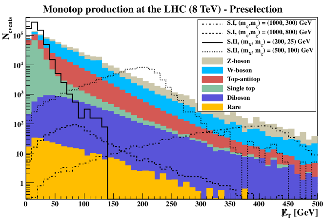
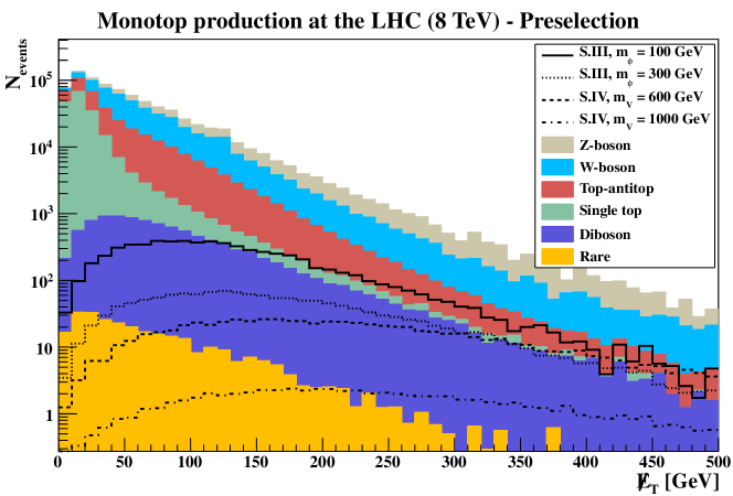
Figure 7.5: Missing transverse energy distributions after preselecting events containing exactly one single $b$-tagged jet, two or three light jets and no isolated charged leptons. We distinguish the various contributions to the Standard Model background and present results for the production of $Z$-boson (gray), $W$-boson (blue), top-antitop pairs (red), single top (green) and diboson (mauve) in association with jets, as well as those related to rarer Standard Model processes (orange). Predictions for four representative signal scenarios of class S.I and S.II are superimposed to the Standard Model expectation for different choices of resonance and invisible particle masses on the upper panel of the figure while the lower panel addresses scenarios of class S.III and S.IV. The coupling strengths are taken as $a=0.1$ in all cases.

As already mentioned in Ref. [142], a simple selection on the missing energy is expected to be sufficient to suppress most of the background. This is illustrated on Figure 7.5 where we present the missing transverse energy distribution for the different background contributions as well as for a small set of representative signal scenarios. On the upper panel of the figure, we address scenarios of type S.I and S.II where the monotop signature arises from the decay of a resonance. We choose four scenarios depicting features associated with different regions of the parameter space. Two of the benchmark points are of class S.I and exhibit a heavy scalar resonant state of mass $m_{\varphi}=1000$ GeV. The invisible fermion is then either moderately light ($m_{\chi}=300$ GeV) or rather heavy ($m_{\chi}=800$ GeV). In the first case, the available phase space for the decay into a monotop state is important while in the second case, the monotop system has to be produced almost at threshold. The two last illustrative scenarios are of type S.II with a rather light vector resonance of mass $m_{X}=200$ GeV and $m_{X}=500$ GeV, respectively. For the first scenario, the mass of the invisible particle must be chosen very light ($m_{\chi}=25$ GeV) in order to allow the resonance to decay into a monotop state, while in the second one, its mass is taken more moderately, $m_{\chi}=100$ GeV. Investigating the missing energy distributions shown in the figure, we observe a typical resonant behavior, the spectrum showing an edge (distorted due to detector effects) at a value depending both on the mass of the resonance and on the one of the invisible particle. For larger mass differences, and in particular for very heavy resonances, the missing energy spectrum extents to larger values. This suggests a key event selection criterion requiring an important quantity of missing energy which would yield the rejection of most of the Standard Model background and allow us to keep a large fraction of the signal events. In contrast, when the resonance mass is close to the sum of the top mass and the invisible particle mass, the position of the edge of the spectrum lies at lower missing energy values, which renders the observation of such a monotop state challenging due to the much larger Standard Model background. We therefore design two different monotop search strategies, one of them being dedicated to the low mass region with a selection threshold on the missing energy taken as low as possible (but reasonable enough to ensure a good control of the Standard Model background), and another one with a harder selection on the missing energy, expected to be more sensible to the high mass region.

On the lower panel of Figure 7.5, we superimpose to the Standard Model predictions four representative signal scenarios of class S.III and S.IV where the monotop state arises from a flavor-changing interaction. We consider lighter scalar invisible states in the case of S.III scenarios with $m_{\phi}=100$ GeV and $m_{\phi}=300$ GeV and heavier vector invisible state in the context of S.IV scenarios with $m_{V}=600$ GeV and $m_{V}=1000$ GeV. Compared to the resonant case, the distributions are flatter and show a peak whose value depends on the mass of the invisible particle. However, even for small masses, the peak stands already at larger $\not{E}_{T}$ values compared to the Standard Model background. Similarly, a key selection strategy based on the missing energy would allow, in most of the cases, for a good background rejection together with an important signal selection efficiency.

From those considerations, we define two options for a missing energy selection and ask it to satisfy

$$\text{ either }\not{E}_{T}\geq 150\leavevmode\nobreak\ \text{GeV}\qquad\text{or}\qquad\not{E}_{T}\geq 250\leavevmode\nobreak\ \text{GeV}\ .$$ (7.3.1)

The first choice is driven by the missing transverse energy value for which the ATLAS and CMS detectors can trig on with an efficiency greater than 70% [568, 569], assuming the use of missing energy only triggers. Such a low missing energy selection threshold is expected to increase the sensitivity to monotop parameter space regions where the invisible particle is light or, for scenarios of type S.I and S.II, when the intermediate resonance is not that heavy (see Figure 7.5). In contrast, the second choice on the missing transverse energy selection is dedicated to parameter space regions with a heavier invisible particle (but only for benchmark points where the production cross section is large enough) or, in the context of scenarios of class S.I and S.II featuring a heavier resonance. A more stringent missing energy selection is also associated with a trigger efficiency closer to unity for both LHC experiments. Additionally, both choices are also expected to lead to a good control of the non-simulated multijet background, together with the current preselection [142, 530, 531].

After imposing $\not{E}_{T}\geq 150$ GeV, about 45000 background events are found to survive, most of them being related to the production of an invisibly decaying $Z$-boson (43%), a $W$-boson (37%) or a top-antitop pair (15%) with jets. With the harder selection on the missing energy $\not{E}_{T}\geq 250$ GeV, only about 8000 background events remain. In this case, the three main sources of Standard Model background consist of events associated with the production of a $Z$-boson (53%), a $W$-boson (33%) or of a top-antitop pair (8%) in association with jets.

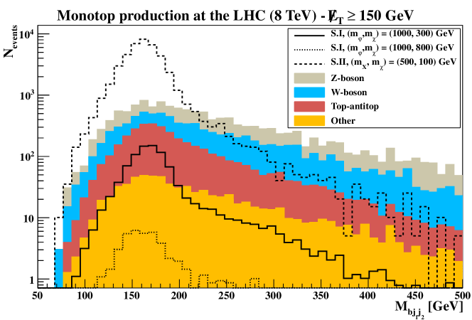
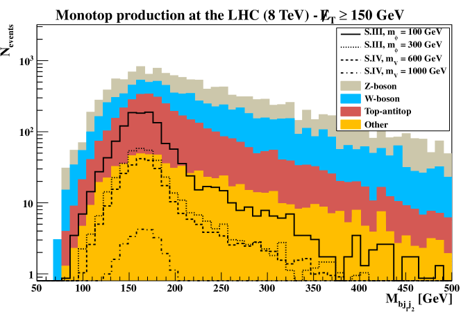
Figure 7.6: Invariant mass distribution of the three-jet system comprised of the $b$-tagged jet and the two light jets defined as originating from a $W$-boson decay, after applying the selection strategy described in the text with a missing transverse energy requirement of $\not{E}_{T}\geq 150$ GeV. We distinguish the various dominant contributions to the Standard Model background and present results for $Z$-boson (gray), $W$-boson (blue) and top-antitop pairs (red) production in association with jets, as well as those related to other Standard Model processes contributing in a smaller extent (orange). Predictions for four representative signal scenarios of class S.I and S.II are superimposed to the Standard Model expectation for different choices of resonance and invisible particle masses on the upper panel of the figure while the lower panel addresses scenarios of class S.III and S.IV. The coupling strengths are taken as $a=0.1$ in all cases. There is no event surviving the selection strategy in the case of the fourth signal scenario included in the upper panel of Figure 7.5.

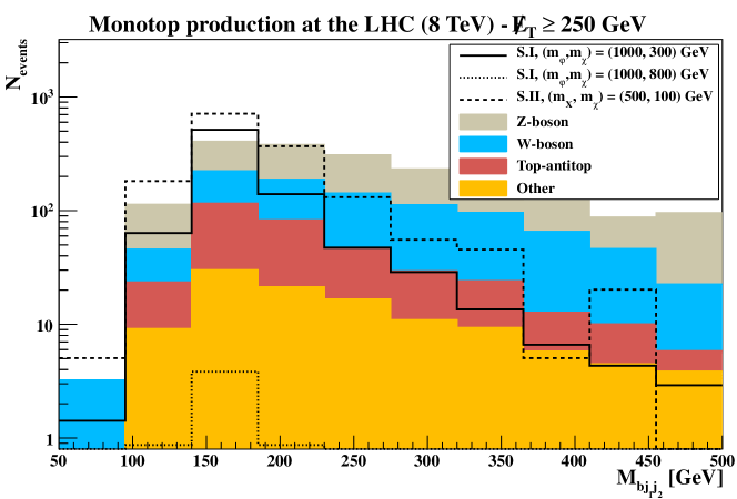
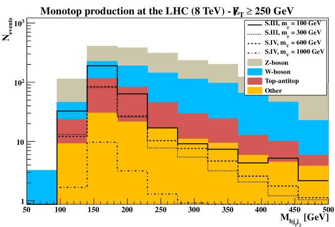
Figure 7.7: Same as in Figure 7.6 but for a missing transverse energy requirement of $\not{E}_{T}\leavevmode\nobreak\ \geq\leavevmode\nobreak\ 250$ GeV.

The next steps of the selection take advantage of the configuration of the final state for signal events. Two of the selected light jets $j_{1}$ and $j_{2}$ must have an invariant mass $m_{j_{1}j_{2}}$ compatible with the mass of a $W$-boson so that we reject events for which

$$m_{j_{1}j_{2}}\ \not{\in}\ [50,105]\leavevmode\nobreak\ \text{GeV}\ .$$ (7.3.2)

In the case of events containing three light jets, we define as $m_{j_{1}j_{2}}$ the invariant mass of the dijet system whose invariant mass is the closest to the $W$-boson mass. In addition, we require the leading jet momentum $\vec{p}(j_{1})$ to be separated from the missing momentum $\vec{\not{p}}_{T}$ in the transverse plane,

$$\Delta\varphi\Big{(}\vec{\not{p}}_{T},\vec{p}(j_{1})\Big{)}\in[0.5,5.75]\ ,$$ (7.3.3)

recalling that $\varphi$ stands for the azimuthal angle with respect to the beam direction. Taking into account the $b$-tagged jet $b$, we reconstruct the top quark as the system comprised of the three jets $j_{1}$, $j_{2}$ and $b$. We first demand that the reconstructed top is well separated from the missing momentum direction,

$$\Delta\varphi\Big{(}\vec{\not{p}}_{T},\vec{p}(t)\Big{)}\in[1,5]\ .$$ (7.3.4)

Background	$N_{\rm events}$, $\not{E}_{T}\geq 150$ GeV	$N_{\rm events}$, $\not{E}_{T}\geq 250$ GeV
$Z$-boson plus jets	$1411\pm 38$	$210\pm 15$
$W$-boson plus jets	$1064\pm 33$	$148\pm 12$
Top-antitop pair plus jets	$1486\pm 39$	$105\pm 10$
Other background sources	$262\pm 15$	$34.7\pm 5.9$
Total	$4223\pm 65$	$497\pm 22$

Table 7.4: Number of expected monotop events ($N_{\rm events}$) for 20 fb^-1 of LHC collisions at a center-of-mass energy of 8 TeV, given together with the associated statistical uncertainties. These numbers have been derived after applying all the selections described in the text for two different requirements on the missing transverse energy. We present results for the different contributions to the Standard Model background.

At this stage of the analysis, the Standard Model background consists of about 15000 (2000) events when applying the $\not{E}_{T}\geq 150$ GeV (250 GeV) missing energy requirement and is composed at 40% (52%), 33% (31%) and 22% (11%) of events originating from the production of a $Z$-boson, a $W$-boson and a top-antitop pair, respectively, in association with jets. We illustrate the selection performed so far on Figure 7.6 and Figure 7.7 by presenting the trijet invariant-mass $m_{bj_{1}j_{2}}$ spectrum for the different (dominant) background contributions and a few representative signal scenarios. The first series of figures (Figure 7.6) is dedicated to the analysis strategy with the softer missing energy selection. On the upper panel of the figure, we compare the background expectation to predictions for signal scenarios of class S.I and S.II, whereas the lower panel of the figure addresses scenarios of class S.III and S.IV. Similarly, Figure 7.7 concerns the analysis strategy with the hardest missing energy requirement.

Signal scenario	$N_{\rm events}$, $\not{E}_{T}\geq 150$ GeV	$N_{\rm events}$, $\not{E}_{T}\geq 250$ GeV
S.I, $m_{\varphi}=1000$ GeV, $m_{\chi}=300$ GeV	$664\pm 25$	$581\pm 23$
S.I, $m_{\varphi}=1000$ GeV, $m_{\chi}=800$ GeV	$29.4\pm 5.4$	$4.1\pm 2.0$
S.II, $m_{X}=200$ GeV, $m_{\chi}=25$ GeV	$\approx 0$	$\approx 0$
S.II, $m_{X}=500$ GeV, $m_{\chi}=100$ GeV	$31047\pm 171$	$334\pm 18$
S.III, $m_{\phi}=100$ GeV	$885\pm 29$	$212\pm 15$
S.III, $m_{\phi}=300$ GeV	$268\pm 16$	$92.0\pm 9.5$
S.IV, $m_{V}=600$ GeV	$191\pm 14$	$95.6\pm 9.7$
S.IV, $m_{V}=1000$ GeV	$19.7\pm 4.3$	$11.0\pm 3.3$

Table 7.5: Same as above but for each of the eight representative signal scenarios introduced in this section. The free coupling parameter is chosen in each case as $a=0.1$.

As illustrated on the four subfigures, constraining the invariant mass of the three jet system, or equivalently constraining the reconstructed top mass, can help to reduce the background contamination. We hence enforce the $m_{bj_{1}j_{2}}$ quantity to lie close to the value of the top mass, since contrary to the different signal spectra which present a clear peak centered around the mass of the top quark, the background expectation exhibits a continuum extending to much larger values of the invariant mass $m_{bj_{1}j_{2}}$. We therefore reject events for which

$$m_{bj_{1}j_{2}}\ \not{\in}\ [140,195]\leavevmode\nobreak\ \text{GeV}\ ,$$ (7.3.5)

and obtain the number of events given in Table 7.4 for the different (dominant) contributions to the Standard Model background and in Table 7.5 for the eight representative signal scenarios investigated in details in this section. As already mentioned, resonant scenarios of class S.I and S.II lead to a number of selected events largely depending on both the resonant mass, whose production cross section depends on, and on its difference with the sum of the top mass and the invisible fermion mass which controls the position of the edge in the missing energy distribution. In contrast, flavor-changing monotop production as featured in scenarios of class S.III and S.IV predicts a number of events surviving the selection strategies only depending on the invisible particle mass. In all cases, we have chosen a given value of the coupling strength $a$ fixed to $a=0.1$ for the sake of the example. Results for other values of $a$ can easily be deduced as the number of selected signal events is proportional to $a^{2}$.

We now translate the number of signal ($S$) and background ($B$) events passing all selections in terms of the LHC sensitivity, with 20 fb^-1 of proton-proton collisions at a center-of-mass energy of 8 TeV, to monotops as produced in the context of scenarios of type S.I (upper panel of Figure 7.8), S.II (lower panel of Figure 7.8), S.III (upper panel of Figure 7.9) and S.IV (lower panel of Figure 7.9). In those figures, we define the sensitivity to each benchmark point as the significance $s=S/\sqrt{S+B}$ and present the contour lines where $s=3$ (dotted curves) and $s=5$ (plain curves).

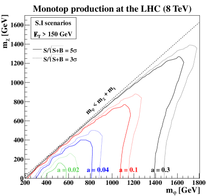
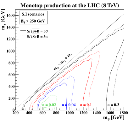
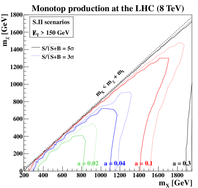
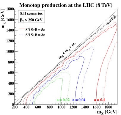
Figure 7.8: LHC sensitivity to monotop production in the context of scenarios of class S.I (upper figures) and S.II (lower figures) with 20 fb^-1 of proton-proton collisions at a center-of-mass energy of 8 TeV. The sensitivity is calculated as the ratio $S/\sqrt{S+B}$ where $S$ is the number of signal events surviving all selections presented in the text. The results, given in the $(m_{\chi},m_{\varphi})$ and $(m_{\chi},m_{X})$ planes for scenarios of class S.I and S.II, respectively, are presented for several values of the coupling parameter $a=0.02$ (green), 0.04 (blue), 0.1 (red) and 0.3 (black). Moreover, we focus on a search strategy based on a missing energy requirement of $\not{E}_{T}\geq 150$ GeV in the left column of the figure, whereas those related to the $\not{E}_{T}\geq 250$ GeV selection are shown in the right column of the figure.

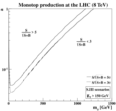
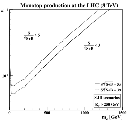
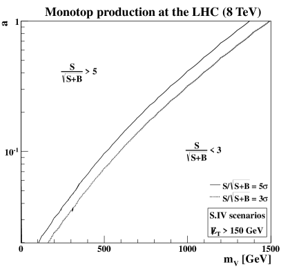
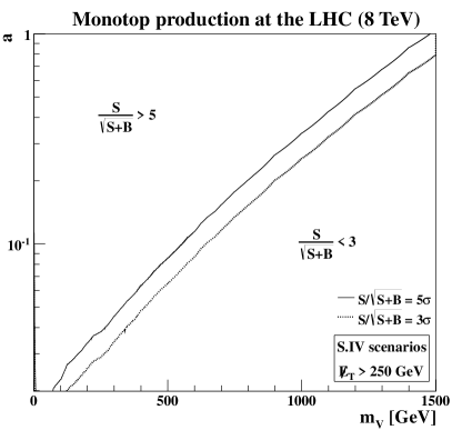
Figure 7.9: Same as in Figure 7.8 but in the context of monotop scenarios of class S.III (upper figures) and S.IV (lower figures). The results are this time given in the $(m_{\phi},a)$ and $(m_{V},a)$ planes for scenarios of class S.III and S.IV, respectively.

On Figure 7.8, we extract the significance as a function of both the resonant and the invisible fermion masses for different values of the coupling strength $a$. We first observe that the LHC is more sensitive to scenarios where the resonance decaying into a monotop state is a vector particle. As already mentioned in Section 7.1.1, this effect is directly related to the larger cross section in scenarios of class S.II for a given choice of masses. Next, it is found that very large coupling values of $a\geq 0.1$ implies a very good coverage of the parameter space by the LHC, both concerning a possible monotop discovery (the $5\sigma$ curves) or the observation of an important deviation (the $3\sigma$ curves) with respect to the Standard Model expectation. In this way, resonance masses ranging up to about 1-1.5 TeV (1.5-2 TeV) are accessible, for invisible particle masses of 800-1300 GeV (1200-1800 GeV) in scenarios of type S.I (S.II). For smaller coupling strengths, the reaches are reduced, although the LHC remains a promising machine for accessing the low mass regions of the parameter space. Finally, comparing the left column of the figure to its right column, we again conclude that a larger missing energy requirement increases the analysis sensitivity to the high mass parameter space regions whereas it simultaneously decrease the sensitivity to the low mass regions.

We recall that we have neglected here the efficiencies of the missing energy only triggers [568, 569]. Even if requiring $\not{E}_{T}\geq 150$ GeV is above the thresholds for both the ATLAS and CMS experiments, the corresponding efficiencies are lower than in the case of a $\not{E}_{T}\geq 250$ GeV selection, which could slightly changes the picture depicted in the figures.

Similar conclusions are found for scenarios of class S.III and S.IV in Figure 7.9. The results are here presented in two-dimensional planes with the invisible particle mass on the $x$-axis ($m_{\phi}$ and $m_{V}$ for scenarios of type S.III and S.IV, respectively) and the coupling strength $a$ on the $y$-axis. In contrast to the resonant case for which there exists no public results for monotop searches at a collider experiment, monotop production induced by a flavor-changing interaction has been searched for by the CDF collaboration in the case the invisible particle is a new vector state [145] (see also Section 8). Limits on the monotop production cross section for masses of the invisible vector particle lying in the range [0, 150] GeV have been extracted from data. The non-observation of any signal event has implied that for a coupling strength of $a=0.1$, benchmark scenarios for which $m_{V}\leq 140$ GeV are excluded. From the curves shown on Figure 7.9, it is clear that future results from monotop analyses at the LHC could greatly improve the current constraints.

7.4 Sgluon-induced multitop production with an ATLAS-like detector

In this section, we use the effective model describing sgluon pair production and decay constructed in Section 7.1.2 to analyze the sensitivity of the LHC through two search strategies, the first one being based on a multilepton plus jets signature and the second one on a single lepton plus jets signature. The Standard Model background contributions are generated as in Section 7.2 and we leave out any further detail from this section. Concerning signal events, they have been simulated by means of the MadGraph 5 program and reweighted so that the production cross section matches the next-to-leading order result [549, 550]. The UFO model files employed with MadGraph 5 have been generated after implementing the model described in Section 7.1.2 into FeynRules. While the leading order set of the CTEQ6 parton density fit is again employed [522], both the renormalization and factorization scales have been fixed to the transverse mass of the sgluon pair. Parton showering, hadronization and tau decays are then handled as in Section 7.2, using the Pythia 6 package and the Tauola program. Finally, detector simulation is performed, both for the signal and the background, by means of the Delphes program, using the public ATLAS card.

7.4.1 Object definitions

Jets are reconstructed using an anti-$k_{T}$ algorithm [525] as provided by the FastJet package [523, 524], the radius parameter being set to $R=0.4$. In addition, we apply a correction factor to the reconstructed jet transverse energy. This allows us to account for magnetic field effects as simulated by Delphes which are known to introduce large bias in energy reconstruction, in particular for jets with a low transverse momentum $p_{T}$ which get their energy spread out within the detector. Denoting by $E_{T}^{\text{(reco)}}$ the reconstructed jet transverse energy and by $E_{T}^{\text{(truth)}}$ the jet transverse energy before detector simulation, we model these effects through the variable

$$\omega=\frac{E_{T}^{\text{(reco)}}-E_{T}^{\text{(truth)}}}{E_{T}^{\text{(truth)}}}\ .$$ (7.4.1)

The evolution of this variable with the (true) jet energy is presented by red squares on Figure 7.10. This figure is based on dijet events originating from the decay of a sequential $Z^{\prime}$-boson, i.e., a massive vector boson with the same couplings to quarks and leptons as the Standard Model $Z$-boson. In order to probe the entire energy range, we have allowed the $Z^{\prime}$ mass to vary in the range [200, 1000] GeV. The energy loss reaches about $5\%$ for low-$p_{T}$ jets with $E_{T}^{\text{(truth)}}=20$ GeV while it stabilizes to about $1\%$ for jets with a transverse energy $E_{T}^{\text{(truth)}}$ larger than 500 GeV.

Figure 7.10: Evolution of the $\omega$-variable defined in Eq. (7.4.1) with respect to the true transverse energy of the reconstructed jet $E_{T}^{\text{(truth)}}$ before (red squares) and after (blue circles) calibration. Figure taken from Ref. [143].

Fitting the distribution, we account for magnetic field effects by an ad-hoc energy calibration. This leads to the application on the reconstructed jet energy of the correction function

$$E_{T}^{\rm(cal)}=\bigg{[}2.62\cdot 10^{-3}-\frac{0.451{\rm GeV}}{E_{T}^{\rm(reco)}}\ln\frac{E_{T}^{\rm(reco)}}{1\leavevmode\nobreak\ {\rm GeV}}\bigg{]}E_{T}^{\rm(reco)}\ ,$$ (7.4.2)

where $E_{T}^{\rm(cal)}$ is the jet transverse energy after calibration and where all the energies are given in GeV. This procedure allows us to recover a correct jet energy for transverse energy as low as $E_{T}^{\text{(truth)}}\sim 40$ GeV, as shown by the blue circles on Figure 7.10.

In our analysis, only jets with a calibrated transverse energy $E_{T}^{({\rm cal})}\geq 20$ GeV and a pseudorapidity $|\eta|\leq 2.5$, are retained. In addition, we estimate a $b$-tagging efficiency of about 60%, while the associated charm and light flavor mistagging rate are assumed to be of about 10% and 1%, respectively.

Charged lepton candidates are requested to have a transverse momentum $p_{T}\geq 20$ GeV and a pseudorapidity $|\eta|\leq 2.47$ and $|\eta|\leq 2.5$ for electrons and muons, respectively. In addition, we also impose two isolation criteria. First, the closest jet to an electron is removed from the event if their relative angular distance $\Delta R=\sqrt{\Delta\varphi^{2}+\Delta\eta^{2}}\leq 0.1$, where $\varphi$ stands for the azimuthal angle with respect to the beam direction. Secondly, in the case at least one jet is present within a cone of radius $R=0.4$ centered on the lepton, the lepton is this time removed.

7.4.2 Searching for sgluons via multitop events at the LHC

In the context of the two classes of scenarios introduced in Section 7.1.2 and summarized in Table 7.1, sgluon pair production and decay lead to three topologies comprised of two top quarks and two light jets ($tjtj$), three top quarks and one light jet ($tjtt$) and four top quarks ($tttt$), denoting top and antitop quarks by the common symbol $t$ and light jets by the symbol $j$. In all channels, the final state is thus characterized by a large number of hard jets (between four and twelve) with an important heavy-flavor content arising from the top decays. We neglect full hadronic channels where each top quark is assumed to decay into a pair of light jets and a single $b$-tagged jet. Although signal cross sections are larger than in the leptonic cases, the overwhelming multijet background, whose a correct treatment requires data-driven methods, renders any signal extraction from the background more challenging, so that we restrict ourselves to leptonic final states, designing two analyses, a first one dedicated to events containing exactly one lepton and a second one to events with at least two leptons.

Event selection strategy for a multilepton plus jets signature

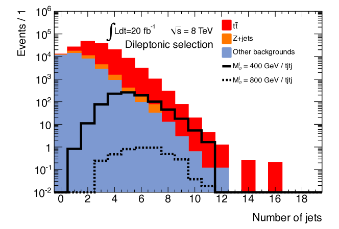
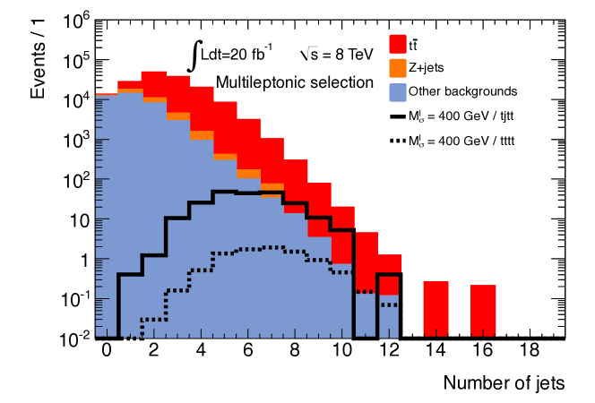
Figure 7.11: Jet multiplicity distribution after selecting events with exactly (upper panel) or at least (lower panel) two leptons, a certain amount of missing transverse energy $\not{E}_{T}\geq 40$ GeV and a dilepton invariant-mass $m_{\ell\ell}\geq 50$ GeV. Contributions arising from top-antitop (red) and Drell-Yan (orange) events are factorized from the rest of the background (blue). Signal distributions for several representative benchmark scenarios are also indicated in the context of the $tjtj$ (upper panel) and the $tjtt$/$tttt$ (lower panel) by plain and dashed curves. Figures taken from Ref. [143].

Events are preselected with the requirement that they contain exactly (for the $tjtj$ topology) or at least (for the other topologies) two charged leptons with a transverse momentum $p_{T}^{\ell}\leavevmode\nobreak\ \geq\leavevmode\nobreak\ 20$ GeV. Moreover, the invariant mass of a lepton pair is imposed to be $m_{\ell\ell}\geq 50$ GeV to remove hadronic resonances decaying into a lepton pair. After this preselection, the Standard Model background contains a large fraction of Drell-Yan dileptonic events (98.7% and 98.2% for the $tjtj$ and $tjtt$/$tttt$ topologies, respectively). To reduce this background, a selection on the missing transverse energy $\not{E}_{T}$, defined as in Eq. (6.4.2), is applied. By only considering events where $\not{E}_{T}\geq 40$ GeV, we take advantage of the fact that Drell-Yan events are characterized by a lack of missing energy, whereas neutrinos arising from leptonic top decays ensure signal events to contain a sensible quantity of missing energy.

Selections	$tjtj$ channel
	$M_{\sigma}^{I}=400$ GeV	$M_{\sigma}^{I}=800$ GeV	Backgrounds
$N_{\ell}=2$ with $p^{\ell}_{T}\geq 20$ GeV	$(1.26\pm 0.02)\!\cdot\!10^{3}$	$4.86\pm 0.30$	$(1.721\pm 0.002)\!\cdot\!10^{7}$
$m_{\ell\ell}\geq 50$ GeV	$(1.15\pm 0.02)\!\cdot\!10^{3}$	$4.49\pm 0.28$	$(1.716\pm 0.002)\!\cdot\!10^{7}$
$\not{E}_{T}\geq 40$ GeV	$(9.38\pm 0.20)\!\cdot\!10^{2}$	$4.04\pm 0.27$	$(1.549\pm 0.004)\!\cdot\!10^{5}$
$N_{j}\geq 3$ with $p^{j}_{T}\geq 25$ GeV	$(9.18\pm 0.19)\!\cdot\!10^{2}$	$4.04\pm 0.27$	$(5.693\pm 0.020)\!\cdot\!10^{4}$
$N_{b}\geq 1$	$(6.05\pm 0.16)\!\cdot\!10^{2}$	$2.80\pm 0.22$	$(4.089\pm 0.011)\!\cdot\!10^{4}$
Same sign dilepton	$(2.81\pm 0.11)\!\cdot\!10^{2}$	$1.06\pm 0.14$	$(4.191\pm 0.035)\!\cdot\!10^{3}$

Selections	$tjtt$ channel
	$M_{\sigma}^{I}=400$ GeV	$M_{\sigma}^{I}=800$ GeV	Backgrounds
$N_{\ell}\geq 2$ with $p^{\ell}_{T}\geq 20$ GeV	$(2.89\pm 0.11)\!\cdot\!10^{2}$	$4.71\pm 0.17$	$(1.722\pm 0.002)\!\cdot\!10^{7}$
$m_{\ell\ell}\geq 50$ GeV	$(2.63\pm 0.10)\!\cdot\!10^{2}$	$4.44\pm 0.17$	$(1.717\pm 0.002)\!\cdot\!10^{7}$
$\not{E}_{T}\geq 40$ GeV	$(2.17\pm 0.09)\!\cdot\!10^{2}$	$4.12\pm 0.16$	$(1.598\pm 0.004)\!\cdot\!10^{5}$
$N_{j}\geq 4$ with $p^{j}_{T}\geq 25$ GeV	$(1.97\pm 0.09)\!\cdot\!10^{2}$	$4.03\pm 0.16$	$(2.375\pm 0.012)\!\cdot\!10^{4}$
$N_{b}\geq 2$	$83.0\pm 6.0$	$1.89\pm 0.11$	$(5.950\pm 0.040)\!\cdot\!10^{3}$
Same sign dilepton	$36.0\pm 4.0$	$0.77\pm 0.07$	$(2.860\pm 0.080)\!\cdot\!10^{2}$

Selections	$tttt$ channel
	$M_{\sigma}^{I}=400$ GeV	$M_{\sigma}^{II}=800$ GeV	Backgrounds
$N_{\ell}\geq 2$ with $p^{\ell}_{T}\geq 20$ GeV	11.33 $\pm$ 0.33	7.90 $\pm$ 0.24	$(1.722\pm 0.002)\!\cdot\!10^{7}$
$m_{\ell\ell}\geq 50$ GeV	10.42 $\pm$ 0.32	7.56 $\pm$ 0.22	$(1.717\pm 0.002)\!\cdot\!10^{7}$
$\not{E}_{T}\geq 40$ GeV	8.78 $\pm$ 0.30	7.03 $\pm$ 0.21	$(1.598\pm 0.004)\!\cdot\!10^{5}$
$N_{j}\geq 5$ with $p^{j}_{T}\geq 25$ GeV	7.50 $\pm$ 0.27	6.60 $\pm$ 0.20	$(8.11\pm 0.06)\!\cdot\!10^{3}$
$N_{b}\geq 3$	1.61 $\pm$ 0.13	1.93 $\pm$ 0.11	$(1.88\pm 0.06)\!\cdot\!10^{2}$
Same sign dilepton	0.69 $\pm$ 0.08	0.82 $\pm$ 0.07	10.3 $\pm$ 1.5

Table 7.6: Flow charts of the number of events surviving the multilepton selection strategy described in the text for the $tjtj$ (upper panel), $tjtt$ (middle panel) and $tttt$ (lower panel) topologies, in the context of the LHC collider running at a center-of-mass energy of $\sqrt{s}=8$ TeV and for an integrated luminosity of 20 fb^-1. We indicate, in addition, the associated statistical uncertainties. For the $tjtj$ and $tjtt$ channels, the signal event numbers correspond to scenarios of class S.I with a sgluon mass of $M_{\sigma}^{I}=400$ GeV and 800 GeV (second and third column of the tables). Concerning the $tttt$ channel, we respectively present instead the evolution of the number of signal events for a scenario of class S.I with a sgluon mass of $M_{\sigma}^{I}=400$ GeV (second column of the last table) and for a scenario of class S.II with a sgluon mass $M_{\sigma}^{II}=800$ GeV (third column of the last table). The sum over all background contributions leads to the event numbers shown in the last column of the tables.

On different footings, jets present in signal events originate mainly from the hadronization of the decay products of the top quarks. In contrast, the hadronic activity in background events is mostly issued from initial-state radiation that leads to a lower jet multiplicity. This is illustrated in Figure 7.11 where we distinguish purely dileptonic final state arising from $tjtj$ events (upper panel of the figure) from signatures possibly containing more than two leptons as induced by $tjtt$ and $tttt$ events (lower panel of the figure). To simultaneously maintain a good sensitivity to the signal and to discard a substantial part of the background, the presence of at least three, four and five jets with $p_{T}^{j}\geq 25$ GeV is demanded for the $tjtj$, $tjtt$ and $tttt$ final states, respectively. In addition, we benefit from the presence of heavy-flavor jets arising from the fragmentation of long-lived $b$-quarks issued from top decays, requiring respectively at least one, two and three $b$-tagged jets for the $tjtj$, $tjtt$ and $tttt$ search channels.

After applying the above-mentioned requirements to the preselected events, the signal selection efficiencies, computed from the information indicated in Table 7.6 containing the number of events surviving each step of the analysis, are found to range from 15% to 50% for a sgluon mass of $M_{\sigma}=400$ GeV (scenario of class S.I) and from 25% to 60% for $M_{\sigma}=800$ GeV (scenario of class S.I for the $tjtj$ and $tjtt$ topologies and of class S.II for the four-top channel). At this stage of the analysis, the Standard Model background has been divided by a factor of about 400, 3000 and 100000 for the $tjtj$, $tjtt$ and $tttt$ search strategies, respectively, and is now largely comprised of Drell-Yan and top-antitop (plus possibly one or two additional gauge bosons) events. We therefore apply a specific selection on the dileptonic events and retain only those where the leptons have the same electric charge. The signal efficiency of such a criterion is of about 50% while only 10% and 20% of the background events survive in the context of the $tjtj$ and $tjtt$/$tttt$ topologies. As a consequence, the background is eventually dominated by top-antitop events for all three search channels, as well as by events related to the associated production of a top-antitop pair with one or two additional gauge bosons in the case of the $tttt$ search strategy.

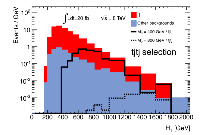
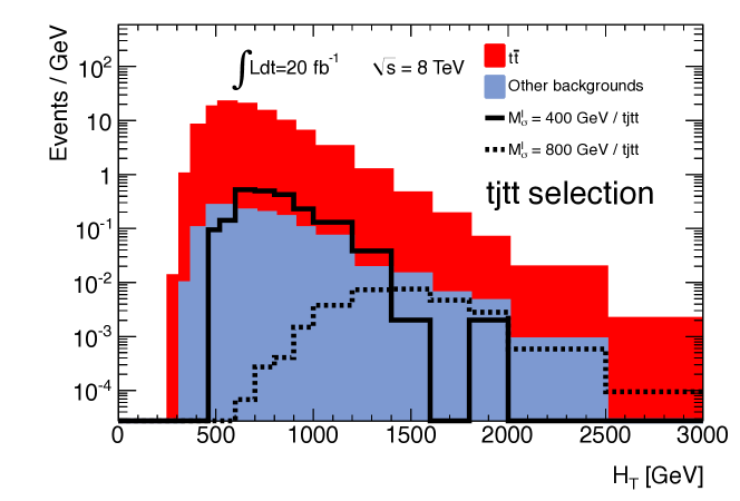
Figure 7.12: Distribution of the $H_{T}$ variable defined in Eq. (6.5.1) after applying the selection strategy presented in Table 7.6 for the $tjtj$ (upper panel) and $tjtt$ (lower panel) topologies. We distinguish the dominant source of background related to the production of $t\bar{t}$ pairs in association with jets (red) from all the other contributions (blue). We superimpose the distributions obtained for two signal scenarios of class S.I with respective sgluon mass of 400 GeV (plain) and 800 GeV (dashed). Figures taken from Ref. [143].

However, the multijet background, jets faking leptons and charge misidentification have not been accounted for in our simulation setup, as already stated above. Recently, the ATLAS collaboration has shown that after a selection strategy very similar to the one performed in this work, neglecting these effects leads to an underestimation of the background contributions by a factor of ten [532]. We therefore adopt a conservative approach and derive below two limits on sgluon-induced new physics in multitop events. First, limits are extracted after omitting the non-simulated background contributions. Next, they are derived after multiplying the number of background events by a factor of ten.

Since signal events are expected to contain more jets and leptons than background events, we consider the $H_{T}$ variable defined by Eq. (6.5.1) to discriminate signal from background. Omitting the $tttt$ channel as its statistical significance is very poor (see Table 7.6 for two illustrative benchmark scenarios), we respectively present $H_{T}$ distributions for the $tjtj$ and $tjtt$ topologies on the upper and lower panels of Figure 7.12. We depict curves associated with signal scenarios of class S.I where the sgluon mass is fixed to 400 GeV and 800 GeV, as in Table 7.6. The distributions present a steep rise once the production threshold is reached, followed by a large peak centered around twice the sgluon mass. We compare these curves to the background distributions, which are indicated after having factorized the dominant $t\bar{t}$ contribution (in red) from the rest of the background events (in blue). The large differences among the shapes of background and signal distributions suggest us to probe the LHC sensitivity to the presence of sgluon fields coupling dominantly to top quarks by means of this $H_{T}$ observable, using the full spectrum rather than applying an (inefficient) selection (see below).

Event selection for a single lepton plus jets signature

The branching ratios of the $tjtj$ and $tjtt/tttt$ topologies into states with one single lepton are large and reach 36% and about $41\%$, respectively. Therefore, events with a single lepton are expected to be copiously produced at the LHC from the production and decay of a sgluon pair. To probe the sensitivity to such a signature, we preselect events by demanding exactly one charged lepton with a transverse momentum $p_{T}^{\ell}\geq 25$ GeV. In this case, the background from the Standard Model is dominated at $92\%$ by events originating from the associated production of a $W$-boson with jets. We illustrate the effect of such a selection on the signal by choosing representative scenarios with sgluon masses of 400 GeV and 800 GeV, like in the previous subsection. The results are presented in Table 7.7 where it is shown that the expected number of signal events ranges from 34.6 (23.2) to 10600 (45.7) for a sgluon mass of 400 GeV (800 GeV).

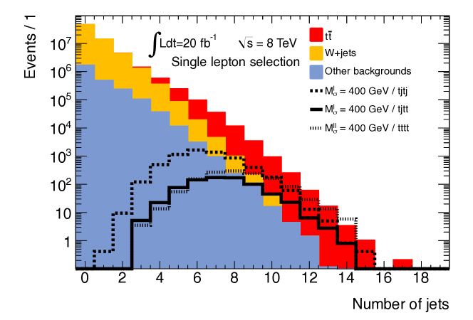
Figure 7.13: Jet multiplicity distribution after selecting events with exactly one lepton, $\not{E}_{T}\leavevmode\nobreak\ \geq\leavevmode\nobreak\ 40$ GeV and $M_{T}^{W}\geq 25$ GeV. We distinguish the $t\bar{t}$ (red) and $W$-boson plus jets (orange) contributions from the rest of the background (blue). We then superimpose signal distributions related to pair production of 400 GeV sgluons, the latter coupling universally to all up-type quarks (scenario of class S.I) in the $tjtj$ (plain), $tjtt$ (strong dashed) and $tttt$ (light dashed) channels. Figure taken from Ref. [143].

Multijet background contributions have not been accounted for in our simulation setup and we need to remedy that lack. To this aim, we rely on data-driven methods such as those introduced in the analysis of Ref. [570]. The latter shows that selecting events with a missing transverse energy larger than $\not{E}_{T}\geq 40$ GeV and requiring the reconstructed $W$-boson transverse mass,

$$M_{T}^{W}=\sqrt{2p_{T}^{\ell}\not{E}_{T}\Big{[}1-\cos\Delta\varphi(\ell,\not{E}_{T})\Big{]}}\ ,$$ (7.4.3)

to be larger than 25 GeV ensure a good control of that source of background. In the equation above, we have introduced the quantity $\Delta\varphi(\ell,\not{E}_{T})$ standing for the angular distance, in the azimuthal direction with respect to the beam, between the lepton and the missing energy.

As in the multilepton analysis, signal events are expected to be rich in hard jets which arise from the hadronization of the decay products of the top quarks. This contrasts with the dominant $W$-boson plus jets background contributions where jets originate mainly from initial-state radiation (see Figure 7.13). Events are therefore selected with the requirement that they contain at least six, seven and eight jets with a transverse-momentum $p_{T}^{j}\geq 25$ GeV in the context of the searches in the $tjtj$, $tjtt$ and $tttt$ topologies, respectively. For the same reasons, signal events are also expected to include a high number of $b$-tagged jets. We therefore demand a minimal number of one and two $b$-jets for the $tjtj$ and $tjtt$/$tttt$ search channels, respectively. At this stage, the expected Standard Model background is composed mainly of $t\bar{t}$ events, the top-antitop pair being possibly produced in association with one or several gauge bosons.

Selections	$tjtj$ channel
	$M_{\sigma}^{I}=400$ GeV	$M_{\sigma}^{I}=800$ GeV	Backgrounds
$N_{\ell}=1$ with $p^{\ell}_{T}\geq 25$ GeV	$(1.06\pm 0.01)\!\cdot\!10^{4}$	$45.7\pm 0.9$	$(2.376\pm 0.003)\!\cdot\!10^{8}$
$\not{E}_{T}\geq 40$ GeV	$(7.65\pm 0.06)\!\cdot\!10^{3}$	$37.9\pm 0.8$	$(6.836\pm 0.002)\!\cdot\!10^{7}$
$M_{T}^{W}\geq 25$ GeV	$(6.43\pm 0.05)\!\cdot\!10^{3}$	$30.7\pm 0.7$	$(6.722\pm 0.002)\!\cdot\!10^{7}$
$N_{j}\geq 6$ with$p_{T}^{j}\geq 25$ GeV	$(3.88\pm 0.04)\!\cdot\!10^{3}$	$24.9\pm 0.7$	$(8.634\pm 0.024)\!\cdot\!10^{4}$
$N_{b}\geq 1$	$(2.91\pm 0.04)\!\cdot\!10^{3}$	$19.3\pm 0.6$	$(6.407\pm 0.014)\!\cdot\!10^{4}$

Selections	$tjtt$ channel
	$M_{\sigma}^{I}=400$ GeV	$M_{\sigma}^{I}=800$ GeV	Backgrounds
$N_{\ell}=1$ with $p^{\ell}_{T}\geq 25$ GeV	$(1.21\pm 0.22)\!\cdot\!10^{3}$	$21.3\pm 0.4$	$(2.376\pm 0.001)\!\cdot\!10^{8}$
$\not{E}_{T}\geq 40$ GeV	$(8.81\pm 0.19)\!\cdot\!10^{2}$	$18.1\pm 0.3$	$(6.836\pm 0.002)\!\cdot\!10^{7}$
$M_{T}^{W}\geq 25$ GeV	$(7.66\pm 0.18)\!\cdot\!10^{2}$	$15.4\pm 0.3$	$(6.722\pm 0.002)\!\cdot\!10^{7}$
$N_{j}\geq 7$ with $p_{T}^{j}\geq 25$ GeV	$(4.05\pm 0.13)\!\cdot\!10^{2}$	$11.08\pm 0.3$	$(2.613\pm 0.012)\!\cdot\!10^{4}$
$N_{b}\geq 2$	$(1.99\pm 0.09)\!\cdot\!10^{2}$	$5.99\pm 0.2$	$(9.330\pm 0.050)\!\cdot\!10^{3}$

Selections	$tttt$ channel
	$M^{I}_{\sigma}\ =\ 400$ GeV	$M^{II}_{\sigma}=800$ GeV	Backgrounds
$N_{\ell}=1$ with $p^{\ell}_{T}\geq 25$ GeV	$34.6\pm 0.6$	$23.2\pm 0.4$	$(2.376\pm 0.001)\!\cdot\!10^{8}$
$\not{E}_{T}\geq 40$ GeV	$27.3\pm 0.5$	$20.2\pm 0.4$	$(6.836\pm 0.002)\!\cdot\!10^{7}$
$M_{T}^{W}\geq 25$ GeV	$23.6\pm 0.5$	$17.1\pm 0.3$	$(6.722\pm 0.002)\!\cdot\!10^{7}$
$N_{j}\geq 8$ with $p_{T}^{j}\geq 25$ GeV	$10.8\pm 0.3$	$12.3\pm 0.3$	$(7.020\pm 0.060)\!\cdot\!10^{3}$
$N_{b}\geq 2$	$7.21\pm 0.27$	$8.47\pm 0.23$	$(2.658\pm 0.026)\!\cdot\!10^{3}$

Table 7.7: Same as Table 7.6 but for a final state signature with one single lepton. We refer to the text for a detailed description of the selection strategy.

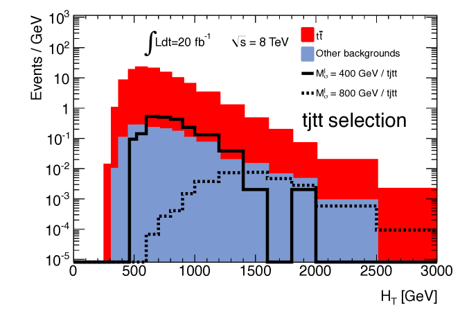
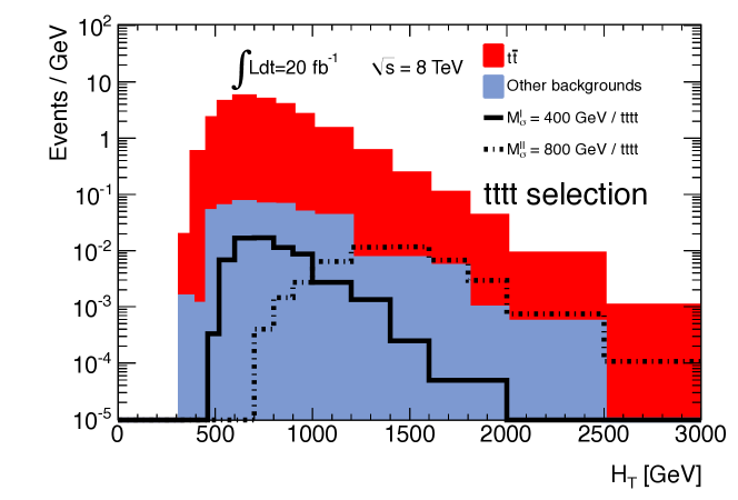
Figure 7.14: Distribution of the hadronic energy $H_{T}$, defined in Eq. (6.5.1), after the selection strategy presented in Table 7.7. We distinguish background events issued from the production of a top-antitop pair together with jets (red) from the other Standard Model contributions (blue). For the $tjtt$ topology (left panel), we superimpose the curves related to two signal scenarios of class S.I with respective sgluon masses of 400 GeV (plain) and 800 GeV (dashed), while for the $tttt$ search strategy (right panel), we consider a scenario of class S.I with a sgluon mass of 400 GeV (plain) and a scenario of class S.II with a sgluon mass of 800 GeV (dashed).

Details on the number of events surviving each of the selection criteria are given in Table 7.7 for two representative signal scenarios with $M_{\sigma}=400$ GeV and 800 GeV as well as for the sum of the background contributions. After all selections, we predict 7.21 (8.47) to 2910 (19.3) signal events, depending on the search channel and for a sgluon mass of 400 (800) GeV. In contrast, the Standard Model expectation consists of 64070, 9330 and 2658 events for the $tjtj$, $tjtt$ and $tttt$ topologies, respectively. The large hadronic activity proper to signal events motivates us to again consider the $H_{T}$ variable as discriminant between signal and background. This feature is depicted on Figure 7.14 in the context of the $tjtt$ (upper panel) and $tttt$ (lower panel) selection strategies. Signal distributions present a clear peaky behavior centered around a $H_{T}$ value of about $1.5M_{\sigma}$ and a tail which does not extend to very large hadronic energies, in contrast to the Standard Model results. The latter, for which we distinguish events associated with top-antitop production in association with jets (red) from the other contributions (blue), show a steep rise once the top-antitop production threshold is reached followed by a peak around $H_{T}\approx 500$ GeV and a smooth fall with increasing energy. This shape difference will be employed below to probe the sgluon mass possibly reachable at the LHC.

While the $H_{T}$ variable is in principle a good discriminant between signal and background, better limits on the sgluon mass can be extracted in the case of the $tjtj$ channel after a kinematical fit of the events, assuming that the missing energy is only originating from a leptonic $W$-boson decay. Assigning the labeling of the six jets according to

$$pp\to\sigma\sigma\to(tj_{5})(tj_{6})\to(j_{1}j_{2}j_{3}j_{5})(j_{4}\ell\nu j_{6})\ ,$$ (7.4.4)

the true configuration of each event is defined as the jet permutation minimizing the $\chi^{2}$-variable

$$\begin{split}\chi^{2}=&\ \left[\frac{m_{j_{1}j_{2}}-m^{(r)}_{W}}{\sigma^{(r)}_{W}}\right]^{2}+\left[\frac{\big{(}m_{j_{1}j_{2}j_{3}}-m_{j_{1}j_{2}}\big{)}-m^{(r)}_{tW}}{\sigma^{(r)}_{tW}}\right]^{2}+\left[\frac{m_{\ell\nu j_{4}}-m^{(r)}_{t\ell}}{\sigma^{(r)}_{t\ell}}\right]^{2}+\\ &\ \left[\frac{(m_{\ell\nu j_{4},j_{6}}-m_{\ell\nu j_{4}})-(m_{j_{1}j_{2}j_{3},j_{5}}-m_{j_{1}j_{2}j_{3}})}{\sigma_{\sigma t}^{(r)}\big{[}(m_{\ell\nu j_{4},j_{6}}-m_{\ell\nu j_{4}})+(m_{j_{1}j_{2}j_{3},j_{5}}-m_{j_{1}j_{2}j_{3}})\big{]}}\right]^{2}\ .\end{split}$$ (7.4.5)

The different contributions to this $\chi^{2}$-variable exactly mimic the decay chain of Eq. (7.4.4). With the first two terms, we ensure that the three jets $j_{1}$, $j_{2}$ and $j_{3}$ consist of the decay products of a hadronically decaying top quark. More into details, they enforce the invariant mass of the first two jets $m_{j_{1}j_{2}}$ to be compatible with the $W$-boson mass and the three-jet system invariant mass $m_{j_{1}j_{2}j_{3}}$ to be compatible with the top mass. Since these two observables are correlated, we however subtract from the reconstructed top mass $m_{j_{1}j_{2}j_{3}}$ the reconstructed dijet invariant-mass $m_{j_{1}j_{2}}$ in the second term of Eq. (7.4.5). The values of the $\chi^{2}$ parameters are taken as $m^{(r)}_{W}=80.7$ GeV, $\sigma^{(r)}_{W}=8.9$ GeV, $m^{(r)}_{tW}=90.8$ GeV and $\sigma^{(r)}_{tW}=10.5$ GeV and have been extracted from a fit based on the Monte Carlo truth where each reconstructed object is correctly assigned according to the configuration of Eq. (7.4.4). The values of the widths of ${\cal O}(10\%)$ are compatible with the mass resolution inputted in our detector simulation.

The third term of Eq. (7.4.5) addresses the leptonically decaying top quark and verifies that the invariant mass $m_{\ell\nu j_{4}}$ is compatible with the top mass. The neutrino four-momentum is reconstructed after assuming that the missing energy of the event as well as the identified charged lepton are both issued from a $W$-boson decay. In this way, information on the reconstructed $W$-boson is implicitly included in the $m_{\ell\nu j_{4}}$ term of the $\chi^{2}$ so that there is no need for a dedicated contribution. From the Monte Carlo truth, we have extracted the parameters $m^{(r)}_{tl}=167.8$ GeV and $\sigma^{(r)}_{tl}=19.1$ GeV.

Finally, both the $tj_{5}$ and $tj_{6}$ systems are the decay products of a sgluon field. Therefore, the invariant masses $m_{j_{1}j_{2}j_{3},j_{5}}$ and $m_{\ell\nu j_{4},j_{6}}$ must be compatible with each other, up to the detector resolution. This leads to the last term of Eq. (7.4.5), after subtracting the reconstructed top masses to avoid possible correlations among the different terms of the $\chi^{2}$ and after including an extra factor at the denominator to remove a too strong dependence on the sgluon mass. From the Monte Carlo truth, we derive the numerical value of the parameter $\sigma_{\sigma t}^{(r)}$, found equal to 0.098 GeV.

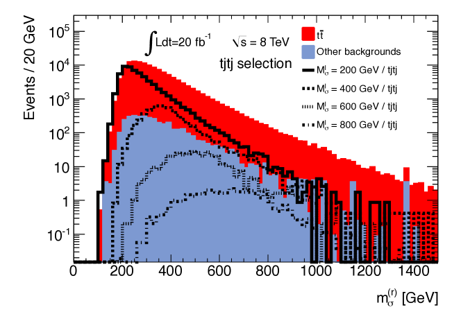
Figure 7.15: Reconstructed sgluon mass $M_{\sigma}^{(r)}$ following the procedure described in the text, after adopting the $tjtj$ search strategy (see the upper panel of Table 7.7). We distinguish the top-antitop contributions (red) from the rest of the background (blue) and superimpose the results associated with four signal scenarios of class S.I, with respective sgluon mass of 200 GeV (plain), 400 GeV (strong dotted), 600 GeV (light dotted) and 800 GeV (dash-dotted). Figure taken from Ref. [143].

After selecting the events as summarized in the upper panel of Table 7.7, we reconstruct each surviving event according to the pattern given in Eq. (7.4.4) by minimizing the $\chi^{2}$-variable of Eq. (7.4.5). We then extract the sgluon mass $M_{\sigma}^{(r)}$ and present the related distributions on Figure 7.15 for both the background, distinguishing the top-antitop pair component (in red) from the other contributions (in blue), and four signal scenarios of class S.I with a sgluon mass of 200 GeV, 400 GeV, 600 GeV and 800 GeV, respectively. The background distribution presents a rising behavior once the top-antitop production threshold is reached, followed by a tail extending up to rather large values of the reconstructed sgluon mass $M_{\sigma}^{(r)}$. In contrast, signal distributions all show a clear peak. For light sgluons ($M_{\sigma}=200$ GeV or 400 GeV), this peak is centered around the true sgluon mass while for heavier sgluons ($M_{\sigma}=600$ GeV and 800 GeV), the detector resolution widens the peak so that the central value is equal to about $70\%-80\%$ of the true sgluon mass. The different shapes of the background and signal distributions can hence be used to extract limits on the sgluon mass possibly reachable at the LHC (see below).

LHC sensitivity to a sgluon field dominantly coupling to top quarks

For each of the considered search channel and strategy, we combine the number of expected signal and background events to calculate upper limits on the signal cross section at the 95% confidence level. More into details, we make use of the CLs technique [571] as implemented in the MCLimit software [572] and employ either the reconstructed sgluon mass (for a $tjtj$ final state with an analysis based on a single lepton signature) or the $H_{T}$ variable (in all the other cases) to discriminate signal from background. The results are presented in Figure 7.16 for the $tjtj$ (upper panel), $tjtt$ (middle panel) and $tttt$ topology (lower panel) as dashed (multilepton analysis), dotted (multilepton analysis after multiplying the background by ten to estimate the effects of the non-simulated contributions) and dot-dashed (single lepton analysis) curves. We also show theoretical predictions for sgluon-induced production of multitop final states as a function of the sgluon mass. In addition to the central next-to-leading order results derived from Table 7.2, we include a $30\%$ uncertainty band corresponding to typical effects induced by factorization and renormalization scale variations (light and dark gray for scenarios of class S.I and S.II, respectively) [549]. In Table 7.8, these results are translated in terms of the sgluon mass that can be possibly excluded at the $95\%$ confidence level for each final state and considered scenario. In addition, $1\sigma$ variations have been derived after accounting for statistical uncertainties.

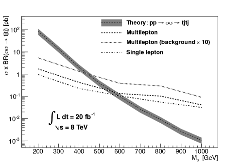
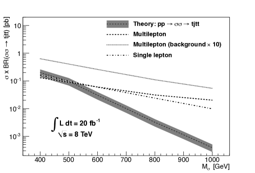
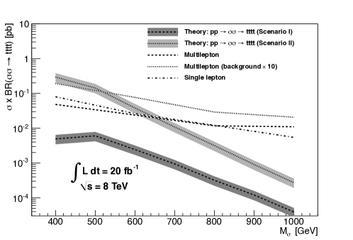
Figure 7.16: The 95% confidence level expected signal cross sections as a function of the sgluon mass, for 20 fb^-1 of LHC collisions at $\sqrt{s}=8$ TeV. The uncertainty bands associated with the next-to-leading order theoretical predictions correspond to 30% variations, as commonly driven by the dependence on the unphysical scales (see Ref. [549]), and are presented as light (dark) gray bands for scenarios of class S.I (S.II). Expected limits in the $tjtj$ (upper), $tjtt$ (middle) and $tttt$ (lower) channels are given as dot-dashed (single lepton analysis), dashed (multilepton analysis) and dotted (multilepton analysis after enhancing the background by a factor of ten) curves. Figures taken from Ref. [143].

	Single lepton analysis	Multilepton analysis	Multilepton analysis
			(background $\times 10$)
$tjtj$	590 ${}^{+40}_{-30}$ GeV	570 ${}^{+30}_{-50}$ GeV	440 ${}^{+40}_{-15}$ GeV
$tjtt$	480 ${}^{+70}_{-80}$ GeV	520 ${}^{+35}_{-90}$ GeV	-
$tttt$ (S.I)	-	-	-
$tttt$ (S.II)	640 ${}^{+40}_{-30}$ GeV	650 ${}^{+30}_{-40}$ GeV	520 ${}^{+50}_{-110}$ GeV

Table 7.8: Expected sensitivity of the LHC, running at a center-of-mass of 8 TeV and for an integrated luminosity of 20 fb^-1, to a sgluon signal in multitop events. The results are given, together with the associated $1\sigma$ statistical uncertainties, in terms of upper bounds on the sgluon mass possibly reachable, at the 95% confidence level, for the different analyses under consideration. Expectations for scenarios of class S.I are given for the $tjtj$, $tjtt$ and $tttt$ channels on the first three lines of the table, respectively. Scenarios of class S.II are only investigated in the context of the $tttt$ search channel, the results being shown on the fourth line of the table.

From the results of the multilepton analysis, we observe that sgluon masses ranging up to 570 GeV and 520 GeV can be excluded by an investigation of the $tjtj$ and $tjtt$ topologies, respectively, in the context of scenarios of class S.I. Equivalently, the LHC, when operating at $\sqrt{s}=8$ TeV, is sensitive to sgluon-induced multitop production cross sections of ${\cal O}(100)$ fb for both signatures. From Table 7.8, it can be seen that the limits obtained for the $tjtj$ search channel vary by less than $10\%$ when accounting for $1\sigma$ statistical uncertainties. In contrast, the bounds extracted from the analysis of the $tjtt$ topology are found to be more sensitive to statistics since they could vary by up to 17% with respect to $1\sigma$ (un)lucky fluctuations. This feature is related to the behavior of both cross sections (including the relevant branching ratios) in the 500-600 GeV sgluon mass range. In the $tjtj$ case, the cross section decreases with the mass, while in the $tjtt$ case, it is rather constant. Due to the low sgluon branching ratio into a top-antitop pair for scenarios of class S.I (see Table 7.2), the multilepton analysis is not sensitive to final states with four top quarks, at least for an integrated luminosity of 20 fb^-1. In class S.II scenarios, this branching ratio is $2.5-7.6$ times more important so that sgluon masses ranging up 650 GeV, or cross sections of ${\cal O}(10)$ fb, can be excluded at the 95% confidence level. When accounting for non-simulated backgrounds by multiplying the number of expected background events by ten, we loose all sensitivity to the $tjtt$ channel while the masses to be possibly excluded when analyzing $tjtj$ and $tttt$ (for scenarios of class S.II) final states decrease from 570 GeV to 440 GeV and from 650 GeV to 520 GeV, respectively.

We now turn to single lepton analyses. First, considering $tjtj$ final states, we show that the reconstructed sgluon mass can be used to exclude at the 95% confidence level sgluon as heavy as 590 GeV, these bounds being rather strong against statistical fluctuations. Next, considering $tjtt$ and $tttt$ topologies, the $H_{T}$ variable is employed as a discriminant and it is found that sgluon masses up to 480 GeV and 640 GeV can be reached. While in the $tjtt$ case, statistical fluctuations can lead to different expectations by about $\pm 15\%$, the results related to a four top signature are found only to change by about $5\%$ within the $1\sigma$ band.

Chapter 8 When theory meets experiment

In the previous chapters of this work, we have investigated two signatures predicted by two non-minimal supersymmetric models. We have addressed the production of a monotop final state, consisting of a single top quark and missing energy, originating from an $R$-parity-violating top squark decay as well as the production of a multitop final state arising from the pair-production and decay of a new scalar state, dubbed sgluon, lying in the adjoint representation of the QCD gauge group. We have then generalized the performed analyses by means of effective field theories in order to facilitate their reinterpretation in the context of various classes of new physics models, supersymmetric or not, although the reinterpretation process in the framework of a well-defined model by itself goes beyond the scope of this work. All the predictions that have been made suggest that the LHC is sensitive to large parts of the respective parameter spaces, which has motivated dedicated ATLAS and CMS searches. These searches are more precisely currently either already achieved [146] or on-going [147, 148]. Furthermore, the obtained results at the phenomenology level have even triggered a first monotop search at the Tevatron collider in 2012 [145].

The above-mentioned LHC and Tevatron experimental analyses have followed the phenomenological studies performed in this work. For obvious reasons, only analyses which are achieved and publicly available are discussed, i.e., a monotop search by the CDF collaboration [145] and an analysis of sgluons decaying into multitop final states performed by the ATLAS collaboration [146]. In the following, the CDF monotop analysis (which is a part of this work) is detailed, from the point of view of a theorist, in Section 8.1 whereas only the conclusions of the ATLAS analysis are presented in Section 8.2.

8.1 Search for monotops with the CDF detector

8.1.1 Analysis strategy for monotop searches with the CDF detector

Among all the scenarios introduced in Section 7.1.1, benchmark points of class S.IV have been considered for a confrontation to data recorded by the CDF detector. In this case, we recall that the top quark is produced in association with an invisible vector field through a flavor-changing interaction of the new state with a top quark and an up quark. In the following, we adopt the CDF notations and the new state, that can in particular be compatible with a dark matter candidate, is denoted by the symbol $D$. The most relevant region of the parameter space with respect to the Tevatron available center-of-mass energy and integrated luminosity consists of the low-mass region. Therefore, the mass of the invisible state $M_{D}$ is further assumed to satisfy

$$M_{D}\in[0-150]\text{\leavevmode\nobreak\ GeV.}$$ (8.1.1)

Such a light dark matter candidate is also motivated by new physics signals reported by several experiments dedicated to direct detection of dark matter. More into details, the DAMA project, based on a detector made up of 250 kg of sodium iodide exploiting the annual modulation of the dark matter signature due to Earth rotation, has first reported an effect that could be explained by a light dark matter candidate [573]. Later, both the CoGeNT experiment, using a low-background germanium detector looking for dark matter elastic interactions with nuclei [574, 575] and the CRESST-II collaboration, probing dark matter detection via its interactions with nuclei inside CaWO₄ crystals [576], have found discrepancies in several observables. It has been found that a by light dark matter particle could explain all the issues. In each of these cases, the light dark matter candidate has to interact with the Standard Model sector in such a way that its detection at collider experiments would be feasible. The classes of scenarios S.III and S.IV designed in the context of the monotop effective field theory of Section 7.1.1 are generic examples of models satisfying these constraints, so that they can also be seen as extensions of the Standard Model with a dark sector coupled to the top quark in a flavor-violating fashion. Consequently, flavor-changing monotop production has received more experimental attention than the resonant one so far.

In this section, we introduce the search strategy designed by the CDF collaboration to probe possible signals of flavor-changing monotop production. This includes 7.7($\pm 0.55$) fb^-1 of events recorded by the CDF-II detector, one of the two general purpose detectors employed for the study of $p\bar{p}$ collisions with a center-of-mass energy of 1.96 TeV at the Tevatron. The CDF-II detector contains a tracking system consisting of a cylindrical open-cell drift chamber together with silicon microstrip detectors immersed in a magnetic field of 1.4 T parallel to the beam axis. This inner part of the detector is surrounded by a calorimetric system comprised of both an electromagnetic and a hadronic piece in order to measure particle energies. Additional drift chambers and muon scintillators are located outside the calorimeters and are dedicated to muon identification. A more detailed description of the detector and the Tevatron accelerating facility can be found in Ref. [577] and references therein.

The results of the monotop analyses of Section 6.4.2 and Section 7.3 at the LHC were suggesting to employ a data acquisition trigger based on the missing energy only. The CDF analysis presented in this section investigates instead events that have triggered the acquisition system by the presence in the final state of two calorimeter clusters together with significant missing transverse energy of at least 35 GeV [578] and 30 GeV [579] for data recorded before and after 2007, respectively. In this case, the missing transverse energy definition relies on calorimetric deposits and is defined as the magnitude of the vectorial sum of the transverse energy contained in each calorimeter tower of the detector.

Jets are reconstructed by making use of the CDF JetClu algorithm [580] using cones of radius $R=0.4$ to cluster calorimeter deposits into jets. Reconstructed jet energies are then corrected using standard techniques developed on the basis of a deep comparison of Monte Carlo simulations of proton-antiproton collisions in CDF and data for several physics processes such as jet, single photon with jets, single gauge boson or $J/\psi$ production [581]. In order to identify jets originating from the fragmentation of a $b$-quark, a secondary-vertex-tagging algorithm is employed, accounting for the longer lifetime of $B$-hadrons [582]. The efficiency of such a $b$-tagging algorithm ranges from 30% to 50% for jets with a transverse energy lower than 200 GeV, for a mistagging rate of a few percents.

In order to achieve a full trigger system efficiency, event selection further requires the amount of missing transverse energy to fulfill

$$\not{E}_{T}\geq 50\text{\leavevmode\nobreak\ GeV}\ .$$ (8.1.2)

In addition only those events whose final state contains exactly three jets are retained. One of these jets is constrained to be identified as a $b$-tagged jet, whereas the transverse energies of the three jets $j_{1}$, $j_{2}$ and $j_{3}$, ordered by decreasing transverse energies, are required to satisfy

$$E_{T}(j_{1})\geq 35\leavevmode\nobreak\ \text{GeV}\ ,\qquad E_{T}(j_{2})\geq 25\leavevmode\nobreak\ \text{GeV}\qquad\text{and}\qquad E_{T}(j_{3})\geq 15\leavevmode\nobreak\ \text{GeV}\ .$$ (8.1.3)

We further impose that either the leading or the next-to-leading jet has a pseudorapidity such that $|\eta|\leq 0.9$, and that all three jets have their pseudorapidity satisfying $|\eta|<2.4$. Finally, events containing any identified charged lepton are vetoed in order to be compatible with the monotop signature associated with a hadronically decaying top quark.

As a consequence of the low missing energy requirement, the event selection gives at this stage a data sample dominated by QCD multijet events with fake missing energy arising from the mismeasurement of jet energies. The simulation of this type of background being prohibitive due to the very large production rate and the important theoretical uncertainties, a QCD multijet sample has instead been generated by using a data-driven method [583]. This method works in several steps. First, a control region enriched in multijet events is defined by restricting the selection (without considering the $b$-tagging requirement) to events with a moderate amount of missing energy (below 70 GeV) and an angular separation smaller than 0.3 between the next-to-leading jet and the missing momentum (multijet events featuring such a quantity of missing energy have often their second jet aligned with the missing momentum). Next, a probability for tagging a jet as a (real or fake) jet issued from a $b$-quark is derived as a function of the hadronic activity of the event and several jet properties such as its transverse momentum and its pseudorapidity. The derived probability is then applied as a per-event weight to all the events satisfying all the selection criteria introduced so far, but the $b$-tagging requirement. The resulting weighted event sample consists of the desired data-driven multijet background once the electroweak contributions, computed by means of Monte Carlo simulations, are subtracted.

All other sources of Standard Model background have been simulated by means of Monte Carlo event generators. Events originating from diboson and top-antitop pair production have been produced using Pythia 6 [45] and reweighted according to the next-to-leading order results as predicted by the Mcfm program for the diboson case [564, 584] and to the approximate next-to-next-to-leading order predictions for the top-antitop case [585]. Furthermore, events issued from single vector boson production in association with (light and heavy flavored) jets have been generated with AlpGen [53], parton showering and hadronization being again performed by pythia, and normalized on the basis of the next-to-leading order cross section returned by Mcfm. Finally, single top events have been modeled with the MadGraph 5 package [64], Pythia 6 taking again care of parton showering and hadronization. Each single top event has then been reweighted according to the next-to-leading order predictions [586, 587].

On different footings, a non-negligible source of background consists of events selected due to the mistagging of a light-flavor jet as a jet issued from a $b$-quark. This contribution is modeled in two stages. As a first step, the mistagging rate of a light jet as a $b$-jet is extracted from data [582]. To this aim, one starts from the secondary vertex that has implied the $b$-tag and calculates the projection onto the jet axis of the vector pointing from the primary to the secondary vertex. This quantity, denoted $L_{2D}$, is dubbed the two-dimensional decay length of the secondary vertex. Its sign plays a critical role in the estimation of the mistagging rate as $b$-quark-initiated hadrons in general lead to large positive values of $L_{2D}$ whereas mistagged lighter jets exhibit smaller $|L_{2D}|$ values that occur with the same rate for both signs. This feature finds its origin in the fact that secondary vertices leading to fake $b$-jets in general arise from tracks found displaced due to tracking errors. However, although decays of $K_{S}$ mesons or $\Lambda$ hyperons contribute subdominantly, their effect is non-negligible and has been considered. True $b$-tagged jet contributions to the negative $L_{2D}$ region are then subtracted by comparing jet data to Monte Carlo simulations, using the distribution of the pseudo-proper decay length $\hat{L}$ defined as

$$\hat{L}=\frac{L_{2D}M^{(v)}}{p_{T}^{(v)}}\ ,$$ (8.1.4)

where $M^{(v)}$ is the invariant mass of all tracks originating from the secondary vertex and $p_{T}^{(v)}$ the transverse-momentum of the secondary vertex four-vector. The quantity $\hat{L}$ turns out to be largely different for $b$-jets and lighter jets and can thus be used as a discriminant. Finally, the mistagging rate in the negative $L_{2D}$ region computed in this way is extrapolated to the positive region. As a second step, the calculated mistagging probability is applied to each light-flavor jet included in the Monte Carlo generated events, the resulting sample being identified as the so-called mistag contributions to the background.

In order to probe the possible presence of monotop events in data, we have simulated eleven signal samples in the framework of the S.IV class of scenarios. The benchmark points differ by the mass $M_{D}$ of the dark matter candidate yielding missing energy. The values for this mass have been chosen by sampling the [0,25] GeV mass range in steps of 5 GeV and the [25,150] GeV range in steps of 25 GeV. Like in the previous sections, signal simulation has been based on the UFO model extracted from the FeynRules implementation of the effective model constructed in Section 7.1.1, after fixing the mass of the top quark to $M_{t}=172.5$ GeV [519, 588]. Hard scattering events have then been generated using the MadGraph 5 package and parton showering and hadronization have been described by the Pythia 6 program.

Applying all the steps of the selection described above, 6471 data events survive. From the Standard Model expectation, it turns out that most of these events (about 70%) consists of QCD multijet events. In this case, as already stated above, the missing momentum tends to be aligned with the momentum of the second jet $j_{2}$. Therefore, a good fraction of the multijet contribution to the background can be rejected by imposing that the azimuthal distance between the missing transverse momentum $\vec{\not{p}}_{T}$ and the momentum of the second hardest jet $\vec{p}(j_{2})$ satisfies

$$\Delta\varphi\Big{(}\vec{\not{p}}_{T},\vec{p}(j_{2})\Big{)}\geq 0.7\ .$$ (8.1.5)

In order to further suppress the Standard Model background, we follow the suggestions of the monotop selection strategy designed in the previous sections and require that the invariant mass of the three-jet system $m_{j_{1}j_{2}j_{3}}$ is compatible with the mass of the top quark,

$$m_{j_{1}j_{2}j_{3}}\in[110,200]\text{\leavevmode\nobreak\ GeV}\ .$$ (8.1.6)

We finally improve the background rejection (without too much affecting the signal selection efficiency) by imposing a large missing transverse energy significance,

$$\frac{\not{E}_{T}}{\sqrt{\sum E_{T}}}\geq 3.5\leavevmode\nobreak\ \sqrt{\text{GeV}}\ ,$$ (8.1.7)

and further constrain the transverse energy of the third jet,

$$E_{T}(j_{3})\geq 25\leavevmode\nobreak\ \text{GeV}\ .$$ (8.1.8)

In Eq. (8.1.7), the expression $\sum E_{T}$ refers to the scalar sum of transverse energy deposited in both calorimeters.

8.1.2 Results of the first monotop search at a hadron collider

Processes	Number of events
Signal scenario with $M_{D}=20$ GeV	2116.9 $\pm$ 121.4
Signal scenario with $M_{D}=75$ GeV	232.3 $\pm$ 22.9
Signal scenario with $M_{D}=100$ GeV	129.8 $\pm$ 12.5
Signal scenario with $M_{D}=125$ GeV	94.5 $\pm$ 9.3
QCD multijet	210.2 $\pm$ 54.5
Top-antitop	182.8 $\pm$ 20.2
Single boson (plus jets)	130.5 $\pm$ 33.8
Mistag	96.9 $\pm$ 39.4
Single top	24.3 $\pm$ 4.5
Diboson	15.7 $\pm$ 2.7
Total background	660.2 $\pm$ 78.1
Data	592

Table 8.1: Number of expected signal (for different masses of the invisible vector particle $M_{D}$) and background events surviving the monotop selection strategy presented in the text, given together with the combined statistical and systematic uncertainties. We distinguish the different background contributions and compare the Standard Model expectation to data.

Although the analysis strategy presented in Section 8.1.1 has been inspired by the phenomenological works of the previous sections, it has more precisely been designed in the aim of optimizing the significance $S/\sqrt{S+B}$, $S$ and $B$ being the expected number of signal and background events, respectively. Out of the 6471 data events, 592 of them remain after the last selection steps. In order to extract some conclusions on the possible presence of monotops in those data, this number must be confronted to the Standard Model predictions. This is achieved in Table 8.1, where we distinguish the different contributions to the Standard Model background and present the number of selected signal events for several simulated scenarios of class S.IV.

The uncertainty values quoted in the table encompass both statistic and systematic uncertainties. For the latter, several contributions have been considered and are listed below. The dominant source of systematic uncertainties consist of the normalization of the QCD multijet background, the mistagging rate of the $b$-tagging algorithm (16.6%) and the theoretical cross sections employed for the different other background contributions ($6.5\%-30\%$). In a smaller extent, uncertainties issued from the jet energy scale ($2.8\%-10.7\%$) [581], the measurement of the luminosity (6%) [589], the efficiency of the $b$-tagging algorithm (5.2%), the initial-state and final-state parton radiation (4%), the parton densities (2%), the veto on the presence of charged leptons in the selection (2%) and the trigger efficiency ($0.4\%-0.9\%$) are included. Finally, two additional sources of systematic uncertainties are also accounted for. A first contribution is derived from the shape variation of various kinematical distributions when a $\pm 1\sigma$ modification of the jet energy scale is performed. On a different line, a second contribution consists of the uncertainties on the efficiency of the data acquisition system.

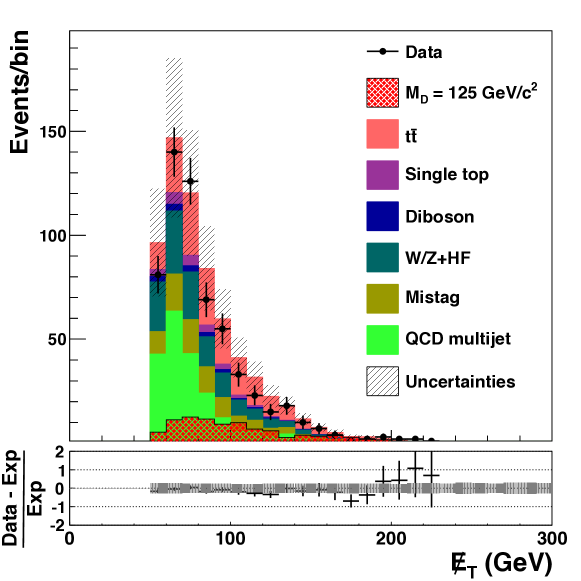
Figure 8.1: Missing transverse energy spectrum after applying the CDF monotop search strategy described in the Section 8.1.1. We compare the sum of the different contributions to the Standard Model background to data and superimpose the expected distribution of a monotop signal arising from a scenario of class S.IV for an invisible particle mass of $M_{D}=125$ GeV. Figure taken from Ref. [145].

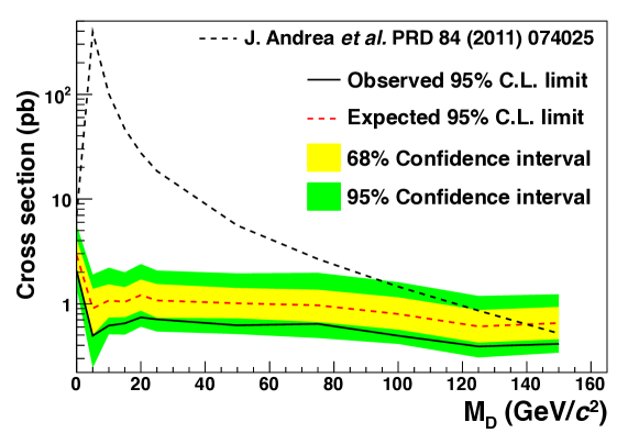
Figure 8.2: Exclusion curve for the monotop production cross section as a function of the mass of the invisible vector particle $M_{D}$. Theoretical cross section extracted from Ref. [142] have been superimposed to the curves. Figure taken from Ref. [145].

One of the key distribution allowing for a signal versus background discrimination in the context of the described monotop search strategy at the Tevatron consists of the missing energy spectrum. This holds in particular for kinematical regions where $\not{E}_{T}$ is large, since in this case, a significant signal contribution is expected together with a reduced background contamination. This is illustrated on Figure 8.1 where we show the different contributions to the Standard Model background and compare their sum to data. In addition, we also present the spectrum induced by the presence of a dark matter particle $D$ of mass $M_{D}=125$ GeV after the selection. The obtained results are compatible with the Standard Model and no significant excess of signal-like events has been found in the analyzed dataset.

Consequently, the results allow to extract 95% confidence level (C.L.) upper limits on the monotop production cross section by comparing the expected shape of the transverse missing energy distribution in the case there is a new physics contribution with the one got from data. To this aim, a Bayesian maximum likelihood method has been employed [590]. The used likelihood function $L$ is defined as the product of Poisson probabilities for each bin of the missing energy distribution. Since the Poisson probabilities are functions of the number of observed data events $d_{i}$ and the predicted number of events $\mu_{i}$ in each bin, we have

$$L=\prod_{i=1}^{n_{\rm bins}}\frac{\mu_{i}^{d_{i}}e^{-\mu_{i}}}{d_{i}\!}\ ,$$ (8.1.9)

where the predictions $\mu_{i}$ have been computed as the sum over both signal and background contributions. In the calculation of the $\mu_{i}$ quantities, a series of nuisance parameters have been introduced, one of them being associated with each source of systematic uncertainties. This allows to calculate predictions for the $\mu_{i}$ quantities encompassing $\pm 1\sigma$ variations possibly induced by the different sources of systematic uncertainties. After assuming Gaussian priors centered on zero and with a unit width for each of the nuisance parameters, the posterior $L^{\prime}$ is computed by marginalizing these parameters, so that it is sufficient to maximize $L^{\prime}$ to get the expected limit on the signal cross section. The 68% and 95% confidence level uncertainty bands are eventually obtained by integrating $L^{\prime}$ over the signal cross section $\sigma_{s}$ varying from zero to infinity when a uniform positive prior is associated with $\sigma_{s}$. The respective bands are then defined by the smallest cross section range containing 68% and 95% of the integral value.

The results are shown on Figure 8.2 as a function of the mass of the new vector state $M_{D}$. In addition, we have indicated the theoretical predictions for the cross section as calculated in the framework of the effective field theory developed in Section 7.1.1, for benchmark scenarios of type S.IV and for a coupling parameter set to $a=0.1$. From the figure, we observe that under the above-mentioned hypotheses, new vector states yielding a monotop signature via flavor-changing interactions are constrained to be heavier than about 100 GeV, at the 95% confidence level.

8.2 Conclusions of a search for sgluons with the ATLAS detector

Using 14.3 fb^-1 of proton-proton collision at a center-of-mass energy of 8 TeV, the ATLAS collaboration has investigated LHC data for hints of sgluon fields dominantly coupling to the top quark, following the work performed in Section 7.4 [146]. In this case, only scenarios of class S.II have been addressed, the sgluon field only singly coupling to a pair of top quarks or gluons. As a result of the analysis, sgluon masses of about 800 GeV have been excluded. Those limits are slightly better than the predictions of Section 7.4 due to a more optimized analysis strategy. As stated at the beginning of this section, we leave any detail of this experimental search out of this work and refer to Ref. [146] for more information.

Chapter 9 Conclusions

The Standard Model of particle physics provides a tremendously successful description of most of currently observed high-energy physics data. However, despite its success, it includes several conceptual problems, such as, e.g., the stabilization of the mass of the recently observed Higgs boson with respect to quantum corrections. This has triggered the construction of a plethora of new physics theories over the last decades whose predict, for most of them, phenomena expected to be observable at scales probed by current and future experiments. In this work, we have focused of one class of such theories dubbed supersymmetry in the aim of investigating specific signatures predicted by non-minimal supersymmetric models at the Large Hadron Collider.

We have started by showing how supersymmetric quantum field theories naturally arise from the only knowledge of both Nœther and spin-statistics theorems used jointly with a series of no-go theorems. We have then described in details how the superspace formalism allows for the construction of supersymmetric Lagrangians in a very efficient way. On different footings, the collider phenomenology of any supersymmetric model can in general be probed after having implemented the Feynman rules associated with the underlying Lagrangian in various high-energy physics tools such as, e.g., Monte Carlo event generators. This has brought us to put some emphasis on the program FeynRules that has been developed over the last few years. It allows, on the one hand, to derive supersymmetric Lagrangians in a very efficient way, and, on the other hand, to extract the related Feynman rules and export them into a programming language that can be understood by Monte Carlo codes. In particular, translating the model into a UFO library offers a way to pass all the information, regardless the use of non-usual Lorentz and/or color structures that could be included in the vertices, to any program lying further in the simulation chain.

Although supersymmetric theories are promising from the theoretical point of view, not a single superpartner has been observed up to now. Therefore, supersymmetry has to be broken so that the masses of the supersymmetric particles are shifted with respect to those of their Standard Model counterparts. We thus depict, in the last formal part of this manuscript, some general properties of broken supersymmetric theories and the most commonly employed mechanisms leading to supersymmetry breaking.

Once these bases have been set, we have moved on with more phenomenological topics. We have detailed the construction of the supersymmetric model resulting from the direct supersymmetrization of the Standard Model, the so-called MSSM, together with its properties. With the current status of the experimental data, designing phenomenologically viable scenarios for the most constrained versions of the MSSM becomes a more and more difficult task. This feature has been illustrated by estimating the regions of the parameter space (un)favored by several low-energy, flavor and electroweak observables as well as by cosmological data and by results of direct searches for supersymmetric particles at colliders. We have in a second stage generalized the squark sector of the minimal model by allowing for non-minimal flavor mixing among all up-type and down-type squark gauge-eigenstates and revisited some of the above-mentioned constraints. We have found that important flavor violation is still allowed by current data, in particular for parameter space regions where the superpartners are heavy.

We have then turned to the building of two non-minimal supersymmetric theories and the detailed investigation of two signatures of such models at the LHC. First, we have illustrated how non-minimal softly-broken supersymmetric theories can be efficiently and easily implemented in FeynRules by using its superspace module and further exported to Monte Carlo event generators for phenomenological investigations at colliders. Next, we have focused on the study of monotop production in the framework of $R$-parity violating supersymmetry and sgluon-induced multitop production within $R$-symmetric supersymmetry. We have chosen two specific benchmark scenarios and show that the LHC is possibly capable of unveiling the presence of new physics within the overwhelming background from the Standard Model through simple search strategies.

However, observing a new physics signal such as those that can arise in the framework of the two investigated benchmark scenarios does neither imply that the relevant scenario consists of the physics model chosen by Nature, nor that the underlying supersymmetric theory is realized. A given signature can be predicted by many benchmarks of a given theory and even by several different theories. In order to allow for an easy recasting of the results into any other context (either another benchmark or another theory beyond the Standard Model), we have followed a bottom-up path starting from the signature itself. In this way, we have constructed one effective field theory for each signature that encompasses all its possible production modes. Consequently, various new physics scenarios yielding either the production of a monotop state or the one of a multitop state issued from the decay of a sgluon pair have been explored simultaneously. Using Monte Carlo simulations of 20 fb^-1 of collisions that have been produced at the LHC in 2012, we have designed general search strategies which we have shown to be sensitive to a large fraction of the effective field theory parameter spaces. It has been found that new physics states lying within the TeV range can easily be observed in most of the cases, for not too small interaction strengths.

Although the reinterpretation of the general results in the framework of a very specific beyond the Standard Model theory is beyond the scope of this work, this consists of its natural extension in a near future. This future can also be seen as the recasting era in particle physics since both the ATLAS and CMS collaborations will certainly not have enough manpower to dedicate (at least) one analysis to each scenario of each new physics theory that theorists can think of, even if we restrict ourselves to scenarios valuable to be investigated. This is the reason why it is likely that both theorists and experimentalists will share this task of reinterpreting the existing searches in the context of large classes of models. In this work, we have shown that several existing tools, such as FeynRules, MadGraph 5 or MadAnalysis 5, are ready to be used for rendering this step more straightforward from the point of view of the user.

In the last part of this work, we have presented one additional example of possible interactions among theorists and experimentalists and described an existing analysis of Tevatron data that has been motivated by our phenomenological results. It consists of a monotop search with the CDF detector at the Tevatron, that we have presented with the eyes of a theorist. We have observed that parameter space regions of the constructed monotop effective field theory, relevant for providing an explanation of observed anomalies in dark matter direct detection experiments, are already excluded by collider data.

Appendix A Conventions

A.1 Lorentz indices

We employ, for the Minkowski metric $\eta_{\mu\nu}$ and its inverse $\eta^{\mu\nu}$, the conventions

$$\eta_{\mu\nu}=\text{diag}(1,-1,-1,-1)\qquad\text{and}\qquad\eta^{\mu\nu}=\text{diag}(1,-1,-1,-1)\ ,$$ (A.1.1)

so that the product of these two symmetric matrices is given by

$$\eta_{\mu\rho}\ \eta^{\rho\nu}=\delta_{\mu}{}^{\nu}\ .$$ (A.1.2)

These matrices allow for lowering and raising spacetime indices,

$$x^{\mu}=\eta^{\mu\nu}x_{\nu}\qquad\text{and}\qquad x_{\mu}=\eta_{\mu\nu}x^{\nu}\ ,$$ (A.1.3)

where $x^{\mu}$ is an arbitrary four-vector. In this work, we use Greek letters from the middle of the alphabet for Lorentz indices ranging from zero to four, and Latin letters from the middle of the alphabet for Euclidean indices ranging from one to three. In our conventions, we define the rank-four antisymmetric tensor with lower indices as

$$\varepsilon_{0123}=1\ .$$ (A.1.4)

Therefore, its counterpart with upper indices is derived as

$$\varepsilon^{\mu\nu\rho\sigma}=\varepsilon_{\tilde{\mu}\tilde{\nu}\tilde{\rho}\tilde{\sigma}}\ \eta^{\mu\tilde{\mu}}\ \eta^{\nu\tilde{\nu}}\ \eta^{\rho\tilde{\rho}}\ \eta^{\sigma\tilde{\sigma}}\ ,$$ (A.1.5)

or equivalently, we have $\varepsilon^{0123}=-1$.

A.2 Spinor indices

For Weyl spinors, we adopt the van der Waerden conventions for indices, so that the tensorial structure of a left-handed Weyl spinor $\lambda$ reads

$$\lambda\equiv\lambda_{\alpha}\ ,$$ (A.2.1)

and the one of a right-handed spinor ${\bar{\chi}}$ is given by

$${\bar{\chi}}\equiv{\bar{\chi}}^{\dot{\alpha}}\ .$$ (A.2.2)

In both cases, we employ Greek letters from the beginning of the alphabet to denote spin indices ranging from one to two. Merging one two-component left-handed Weyl spinor $\lambda_{\alpha}$ and one right-handed two-component Weyl spinor ${\bar{\chi}}^{\dot{\alpha}}$, one constructs four-component Dirac spinors which read, in the van der Waerden notations

$$\psi_{D}=\begin{pmatrix}\lambda_{\alpha}\\ {\bar{\chi}}^{\dot{\alpha}}\end{pmatrix}\ .$$ (A.2.3)

In the case of a four-component Majorana spinor, the left-handed and right-handed components are related by Hermitian conjugation, $(\lambda_{\alpha})^{\dagger}={\bar{\lambda}}_{\dot{\alpha}}$, so that the four-component object reads

$$\psi_{M}=\begin{pmatrix}\lambda_{\alpha}\\ {\bar{\lambda}}^{\dot{\alpha}}\end{pmatrix}\ .$$ (A.2.4)

Getting back to Weyl spinors, their spin indices can be raised and lowered by means of the rank-two antisymmetric tensors $\varepsilon_{\alpha\beta}$ and $\varepsilon^{\alpha\beta}$ acting on left-handed spinors as well as $\varepsilon_{{\dot{\alpha}}{\dot{\beta}}}$ and $\varepsilon^{{\dot{\alpha}}{\dot{\beta}}}$ acting on right-handed spinors. We normalize these tensors as $\varepsilon_{12}=1$, $\varepsilon^{12}=-1$, $\varepsilon_{\dot{1}\dot{2}}=1$ and $\varepsilon^{\dot{1}\dot{2}}=-1$. Subsequently, the summation properties

$$\varepsilon_{\alpha\beta}\,\varepsilon^{\beta\gamma}=\delta_{\alpha}{}^{\gamma}\quad\text{and}\quad\varepsilon_{{\dot{\alpha}}{\dot{\beta}}}\,\varepsilon^{{\dot{\beta}}{\dot{\gamma}}}=\delta_{\dot{\alpha}}{}^{\dot{\gamma}}$$ (A.2.5)

are verified and raising and lowering indices obey the rules

$$\lambda^{\alpha}=\varepsilon^{\alpha\beta}\lambda_{\beta}\ ,\quad\lambda_{\alpha}=\varepsilon_{\alpha\beta}\lambda^{\beta}\ ,\quad{\bar{\chi}}^{\dot{\alpha}}=\varepsilon^{{\dot{\alpha}}{\dot{\beta}}}{\bar{\chi}}_{\dot{\beta}}\quad\text{and}\quad{\bar{\chi}}_{\dot{\alpha}}=\varepsilon_{{\dot{\alpha}}{\dot{\beta}}}{\bar{\chi}}^{\dot{\beta}}\ .$$ (A.2.6)

Contracting spinors with upper and lower indices further allows to define scalar products as

$$\lambda\cdot\lambda^{\prime}=\lambda^{\alpha}\lambda^{\prime}_{\alpha}\quad\text{and}\quad{\bar{\chi}}\cdot{\bar{\chi}}^{\prime}={\bar{\chi}}_{\dot{\alpha}}{\bar{\chi}}^{\prime}{}^{\dot{\alpha}}\ .$$ (A.2.7)

where we have introduced a left-handed Weyl spinor $\lambda^{\prime}$ and a right-handed Weyl spinor ${\bar{\chi}}^{\prime}$.

A.3 Pauli and Dirac matrices

The three Pauli matrices are defined, in our conventions, by

$$\sigma^{1}=\begin{pmatrix}0&1\\ 1&0\end{pmatrix}\ ,\quad\sigma^{2}=\begin{pmatrix}0&-i\\ i&0\end{pmatrix}\quad\text{and}\quad\sigma^{3}=\begin{pmatrix}1&0\\ 0&-1\end{pmatrix}\ ,$$ (A.3.1)

and we remind that $\sigma_{i}=-\sigma^{i}$. Introducing $\sigma^{0}$ as the dimension-two identity matrix, one can construct the two four-vectors

$$\sigma^{\mu}=(\sigma^{0},\sigma^{i})\quad\text{and}\quad{\bar{\sigma}}^{\mu}=(\sigma^{0},-\sigma^{i})\ ,$$ (A.3.2)

whose the tensorial structure reads

$$\sigma^{\mu}\equiv\sigma^{\mu}{}_{\alpha{\dot{\alpha}}}\quad\text{and}\quad{\bar{\sigma}}^{\mu}\equiv{\bar{\sigma}}^{\mu}{}^{{\dot{\alpha}}\alpha}\ .$$ (A.3.3)

From the product of these four-vectors, one gets the generators of the Lorentz algebra in the left-handed and right-handed spinorial representations,

$$\sigma^{\mu\nu}=\frac{i}{4}\Big{[}\sigma^{\mu}{\bar{\sigma}}^{\nu}-\sigma^{\nu}{\bar{\sigma}}^{\mu}\Big{]}\quad\text{and}\quad{\bar{\sigma}}^{\mu\nu}=\frac{i}{4}\Big{[}{\bar{\sigma}}^{\mu}\sigma^{\nu}-{\bar{\sigma}}^{\nu}\sigma^{\mu}\Big{]}\ ,$$ (A.3.4)

respectively. The matrices $\sigma^{\mu}$ and ${\bar{\sigma}}^{\mu}$ naturally appear in superspace computations, together with products of these matrices. The latter can in general be simplified by means of several useful identities. Firstly, the two four-vectors $\sigma^{\mu}$ and ${\bar{\sigma}}^{\mu}$ are related through metric tensors in spin and Minkowski space,

$$\begin{split}{\bar{\sigma}}^{\mu}{}^{{\dot{\beta}}\beta}=\sigma^{\mu}{}_{\alpha{\dot{\alpha}}}\varepsilon^{\alpha\beta}\varepsilon^{{\dot{\alpha}}{\dot{\beta}}}\ ,\qquad&\ \sigma^{\mu}{}_{\alpha{\dot{\alpha}}}{\bar{\sigma}}_{\mu}{}^{{\dot{\beta}}\beta}=2\delta_{\alpha}{}^{\beta}\delta_{\dot{\alpha}}{}^{\dot{\beta}}\ ,\\ {\bar{\sigma}}^{\mu{\dot{\alpha}}\alpha}{\bar{\sigma}}_{\mu}{}^{{\dot{\beta}}\beta}=2\varepsilon^{{\dot{\alpha}}{\dot{\beta}}}\varepsilon^{\alpha\beta}\ ,\qquad&\ \sigma^{\mu}{}_{\alpha{\dot{\alpha}}}\sigma_{\mu}{}_{\beta{\dot{\beta}}}=2\varepsilon_{\alpha\beta}\varepsilon_{{\dot{\alpha}}{\dot{\beta}}}\ ,\\ ({\bar{\sigma}}^{\mu}\sigma^{\nu})^{\dot{\alpha}}{}_{\dot{\beta}}=\eta^{\mu\nu}\delta^{\dot{\alpha}}{}_{\dot{\beta}}-2i({\bar{\sigma}}^{\mu\nu})^{\dot{\alpha}}{}_{\dot{\beta}}\ ,\qquad&\ (\sigma^{\mu}{\bar{\sigma}}^{\nu})_{\alpha}{}^{\beta}=\eta^{\mu\nu}\delta_{\alpha}{}^{\beta}{}-2i(\sigma^{\mu\nu})_{\alpha}{}^{\beta}\ .\end{split}$$ (A.3.5)

Secondly, the tensors $\sigma^{\mu\nu}$ and ${\bar{\sigma}}^{\mu\nu}$ fulfill (anti-)self-duality properties,

$$\frac{1}{2}\varepsilon_{\mu\nu\rho\sigma}\sigma^{\rho\sigma}=-i\sigma_{\mu\nu}\qquad\text{and}\qquad\frac{1}{2}\varepsilon_{\mu\nu\rho\sigma}{\bar{\sigma}}^{\rho\sigma}=i{\bar{\sigma}}_{\mu\nu}\ .$$ (A.3.6)

Finally, the product of three Pauli matrices can be simplified to

$$\begin{split}{\bar{\sigma}}^{\mu}\sigma^{\nu}{\bar{\sigma}}^{\rho}=&\ i\varepsilon^{\mu\nu\rho\sigma}{\bar{\sigma}}_{\sigma}+\eta^{\mu\nu}{\bar{\sigma}}^{\rho}+\eta^{\nu\rho}{\bar{\sigma}}^{\mu}-\eta^{\mu\rho}{\bar{\sigma}}^{\nu}\ ,\\ \sigma^{\mu}{\bar{\sigma}}^{\nu}\sigma^{\rho}=&\ -i\varepsilon^{\mu\nu\rho\sigma}\sigma_{\sigma}+\eta^{\mu\nu}\sigma^{\rho}+\eta^{\nu\rho}\sigma^{\mu}-\eta^{\mu\rho}\sigma^{\nu}\ .\end{split}$$ (A.3.7)

From Pauli matrices, one can construct the Dirac matrices in the Weyl representation,

$$\gamma^{\mu}=\begin{pmatrix}0&\sigma^{\mu}\\ {\bar{\sigma}}^{\mu}&0\end{pmatrix}\ ,$$ (A.3.8)

while products of Dirac matrices define the four-component spinorial representation of the Lorentz algebra

$$\gamma^{\mu\nu}=\frac{i}{4}\big{[}\gamma^{\mu},\gamma^{\nu}\big{]}\ .$$ (A.3.9)

This representation is reducible to the two-component representations defined above so that one can also define a fifth Dirac matrix $\gamma^{5}$ as

$$\gamma^{5}=i\gamma^{0}\gamma^{1}\gamma^{2}\gamma^{3}=\begin{pmatrix}-1&0\\ 0&1\end{pmatrix}\ ,$$ (A.3.10)

which commutes with all the generators of the algebra and which anticommutes with all the Dirac matrices.

A.4 Grassmann variables

A point in superspace is defined by adjoining to the spacetime coordinates $x^{\mu}$ the Grassmann coordinates $\theta_{\alpha}$ and ${\bar{\theta}}^{\dot{\alpha}}$ forming a Majorana spinor. The $\theta$-variables satisfy the Grassmann algebra

$$\big{\{}\theta^{\alpha},\theta^{\beta}\big{\}}=\big{\{}{\bar{\theta}}_{\dot{\alpha}},{\bar{\theta}}_{\dot{\beta}}\big{\}}=\big{\{}\theta^{\alpha},{\bar{\theta}}_{\dot{\alpha}}\big{\}}=0\ .$$ (A.4.1)

Since the square of an anticommuting object vanishes, it follows that

$$\theta^{\alpha}\theta^{\beta}=-\frac{1}{2}\theta\!\cdot\!\theta\varepsilon^{\alpha\beta}\ ,\qquad{\bar{\theta}}^{\dot{\alpha}}{\bar{\theta}}^{\dot{\beta}}=\frac{1}{2}{\bar{\theta}}\!\cdot\!{\bar{\theta}}\varepsilon^{{\dot{\alpha}}{\dot{\beta}}}\qquad\text{and}\qquad\theta^{\alpha}{\bar{\theta}}^{\dot{\alpha}}=\frac{1}{2}\theta\sigma^{\mu}{\bar{\theta}}{\bar{\sigma}}_{\mu}{}^{{\dot{\alpha}}\alpha}\ ,$$ (A.4.2)

which is at the basis of any computation to be performed in superspace. We define the operators $\partial_{\mu}$, $\partial_{\alpha}$ and ${\bar{\partial}}^{\dot{\alpha}}$ conjugate to the superspace coordinates $x^{\mu}$, $\theta^{\alpha}$ and ${\bar{\theta}}^{\dot{\alpha}}$. In other words, we define derivatives with respect to the superspace coordinates that fulfill the properties

$$\big{[}\partial_{\mu},x^{\nu}\big{]}=\delta_{\mu}{}^{\nu}\ ,\qquad\big{\{}\partial_{\alpha},\theta^{\beta}\big{\}}=\delta_{\alpha}{}^{\beta}\qquad\text{and}\qquad\big{\{}{\bar{\partial}}_{\dot{\alpha}},{\bar{\theta}}^{\dot{\beta}}\big{\}}=\delta_{\dot{\alpha}}{}^{\dot{\beta}}\ .$$ (A.4.3)

Finally, integration upon Grassmann variables is defined by the relations

$$\int{\rm d}^{2}\theta=\int{\rm d}^{2}\theta\ \theta=\int{\rm d}^{2}{\bar{\theta}}=\int{\rm d}^{2}{\bar{\theta}}\ {\bar{\theta}}=0\ ,\qquad\int{\rm d}^{2}\theta\ \theta\!\cdot\!\theta=\int{\rm d}^{2}{\bar{\theta}}\ {\bar{\theta}}\!\cdot\!{\bar{\theta}}=1\ .$$ (A.4.4)

References

- [1] S. Glashow, “Partial Symmetries of Weak Interactions,” Nucl.Phys. 22 (1961) 579–588.
- [2] A. Salam and J. C. Ward, “Electromagnetic and Weak Interactions,” Phys.Lett. 13 (1964) 168–171.
- [3] S. Weinberg, “A Model of Leptons,” Phys.Rev.Lett. 19 (1967) 1264–1266.
- [4] A. Salam, Elementary Particle Theory. ed. N. Svartholm (Almqvist and Forlag, Stockholm), 1968.
- [5] S. Glashow, J. Iliopoulos, and L. Maiani, “Weak Interactions with Lepton-Hadron Symmetry,” Phys.Rev. D2 (1970) 1285–1292.
- [6] S. Weinberg, “Mixing Angle in Renormalizable Theories of Weak and Electromagnetic Interactions,” Phys.Rev. D5 (1972) 1962–1967.
- [7] D. Gross and F. Wilczek, “Asymptotically Free Gauge Theories. 1,” Phys.Rev. D8 (1973) 3633–3652.
- [8] M. Kobayashi and T. Maskawa, “CP Violation in the Renormalizable Theory of Weak Interaction,” Prog.Theor.Phys. 49 (1973) 652–657.
- [9] D. Gross and F. Wilczek, “Asymptotically Free Gauge Theories. 2.,” Phys.Rev. D9 (1974) 980–993.
- [10] H. D. Politzer, “Asymptotic Freedom: An Approach to Strong Interactions,” Phys.Rept. 14 (1974) 129–180.
- [11] ATLAS Collaboration, G. Aad et al., “Observation of a New Particle in the Search for the Standard Model Higgs Boson with the ATLAS Detector at the LHC,” Phys.Lett B716 (2012) 1–29.
- [12] CMS Collaboration, S. Chatrchyan et al., “Observation of a New Boson at a Mass of 125 GeV with the CMS Experiment at the LHC,” Phys.Lett B716 (2012) 30–61.
- [13] H. Georgi and S. Glashow, “Unity of All Elementary Particle Forces,” Phys.Rev.Lett. 32 (1974) 438–441.
- [14] H. Georgi, H. R. Quinn, and S. Weinberg, “Hierarchy of Interactions in Unified Gauge Theories,” Phys.Rev.Lett. 33 (1974) 451–454.
- [15] H. Fritzsch and P. Minkowski, “Unified Interactions of Leptons and Hadrons,” Annals Phys. 93 (1975) 193–266.
- [16] F. Gursey, P. Ramond, and P. Sikivie, “A Universal Gauge Theory Model Based on E6,” Phys.Lett. B60 (1976) 177.
- [17] D. Chang, R. Mohapatra, and M. Parida, “A New Approach to Left-Right Symmetry Breaking in Unified Gauge Theories,” Phys.Rev. D30 (1984) 1052.
- [18] E. Witten, “Search for a Realistic Kaluza-Klein Theory,” Nucl.Phys. B186 (1981) 412.
- [19] N. Arkani-Hamed, S. Dimopoulos, and G. Dvali, “The Hierarchy Problem and New Dimensions at a Millimeter,” Phys.Lett. B429 (1998) 263–272.
- [20] L. Randall and R. Sundrum, “A Large Mass Hierarchy from a Small Extra Dimension,” Phys.Rev.Lett. 83 (1999) 3370–3373.
- [21] T. Appelquist, H.-C. Cheng, and B. A. Dobrescu, “Bounds on Universal Extra Dimensions,” Phys.Rev. D64 (2001) 035002.
- [22] Y. Golfand and E. Likhtman, “Extension of the Algebra of Poincare Group Generators and Violation of p Invariance,” JETP Lett. 13 (1971) 323–326.
- [23] D. Volkov and V. Akulov, “Is the Neutrino a Goldstone Particle?,” Phys.Lett. B46 (1973) 109–110.
- [24] J. Wess and B. Zumino, “A Lagrangian Model Invariant Under Supergauge Transformations,” Phys.Lett. B49 (1974) 52.
- [25] J. Wess and B. Zumino, “Supergauge Transformations in Four-Dimensions,” Nucl.Phys. B70 (1974) 39–50.
- [26] J. Wess and B. Zumino, “Supergauge Invariant Extension of Quantum Electrodynamics,” Nucl.Phys. B78 (1974) 1.
- [27] A. Salam and J. A. Strathdee, “Supergauge Transformations,” Nucl. Phys. B76 (1974) 477–482.
- [28] A. Salam and J. A. Strathdee, “On Superfields and Fermi-Bose Symmetry,” Phys.Rev. D11 (1975) 1521–1535.
- [29] S. Ferrara, J. Wess, and B. Zumino, “Supergauge Multiplets and Superfields,” Phys. Lett. B51 (1974) 239.
- [30] S. Ferrara and B. Zumino, “Supergauge Invariant Yang-Mills Theories,” Nucl.Phys. B79 (1974) 413.
- [31] H. P. Nilles, “Supersymmetry, Supergravity and Particle Physics,” Phys.Rept. 110 (1984) 1–162.
- [32] H. E. Haber and G. L. Kane, “The Search for Supersymmetry: Probing Physics Beyond the Standard Model,” Phys.Rept. 117 (1985) 75–263.
- [33] L. E. Ibanez and G. G. Ross, “Low-Energy Predictions in Supersymmetric Grand Unified Theories,” Phys.Lett. B105 (1981) 439.
- [34] S. Dimopoulos, S. Raby, and F. Wilczek, “Supersymmetry and the Scale of Unification,” Phys.Rev. D24 (1981) 1681–1683.
- [35] J. R. Ellis, S. Kelley, and D. V. Nanopoulos, “Probing the Desert Using Gauge Coupling Unification,” Phys.Lett. B260 (1991) 131–137.
- [36] U. Amaldi, W. de Boer, and H. Furstenau, “Comparison of Grand Unified Theories with Electroweak and Strong Coupling Constants Measured at LEP,” Phys.Lett. B260 (1991) 447–455.
- [37] P. Langacker and M.-x. Luo, “Implications of Precision Electroweak Experiments for , , and Grand Unification,” Phys.Rev. D44 (1991) 817–822.
- [38] C. Giunti, C. Kim, and U. Lee, “Running Coupling Constants and Grand Unification Models,” Mod.Phys.Lett. A6 (1991) 1745–1755.
- [39] E. Witten, “Dynamical Breaking of Supersymmetry,” Nucl.Phys. B188 (1981) 513.
- [40] H. Goldberg, “Constraint on the Photino Mass from Cosmology,” Phys.Rev.Lett. 50 (1983) 1419.
- [41] J. R. Ellis, J. Hagelin, D. V. Nanopoulos, K. A. Olive, and M. Srednicki, “Supersymmetric Relics from the Big Bang,” Nucl.Phys. B238 (1984) 453–476.
- [42] https://twiki.cern.ch/twiki/bin/view/AtlasPublic/SupersymmetryPublicResults .
- [43] https://twiki.cern.ch/twiki/bin/view/CMSPublic/PhysicsResultsSUS .
- [44] T. Sjostrand, P. Eden, C. Friberg, L. Lonnblad, G. Miu, et al., “High-Energy Physics Event Generation with PYTHIA 6.1,” Comput.Phys.Commun. 135 (2001) 238–259.
- [45] T. Sjostrand, S. Mrenna, and P. Z. Skands, “Pythia 6.4 Physics and Manual,” JHEP 0605 (2006) 026.
- [46] T. Sjostrand, S. Mrenna, and P. Z. Skands, “A Brief Introduction to Pythia 8.1,” Comput.Phys.Commun. 178 (2008) 852–867.
- [47] T. Gleisberg, S. Hoeche, F. Krauss, A. Schalicke, S. Schumann, et al., “SHERPA 1. Alpha: A Proof of Concept Version,” JHEP 0402 (2004) 056.
- [48] T. Gleisberg, S. Hoeche, F. Krauss, M. Schonherr, S. Schumann, et al., “Event Generation with SHERPA 1.1,” JHEP 0902 (2009) 007.
- [49] G. Corcella, I. Knowles, G. Marchesini, S. Moretti, K. Odagiri, et al., “Herwig 6: An Event generator for hadron emission reactions with interfering gluons (including supersymmetric processes),” JHEP 0101 (2001) 010.
- [50] G. Corcella, I. Knowles, G. Marchesini, S. Moretti, K. Odagiri, et al., “HERWIG 6.5 Release Note,”.
- [51] M. Bahr, S. Gieseke, M. Gigg, D. Grellscheid, K. Hamilton, et al., “Herwig++ Physics and Manual,” Eur.Phys.J. C58 (2008) 639–707.
- [52] K. Arnold, L. d’Errico, S. Gieseke, D. Grellscheid, K. Hamilton, et al., “Herwig++ 2.6 Release Note,”.
- [53] M. L. Mangano, M. Moretti, F. Piccinini, R. Pittau, and A. D. Polosa, “ALPGEN, a Generator for Hard Multiparton Processes in Hadronic Collisions,” JHEP 0307 (2003) 001.
- [54] A. Pukhov, E. Boos, M. Dubinin, V. Edneral, V. Ilyin, et al., “CompHEP: A Package for Evaluation of Feynman Diagrams and Integration over Multiparticle Phase Space,” arXiv:hep-ph/9908288 [hep-ph].
- [55] E. Boos et al., “CompHEP 4.4: Automatic Computations from Lagrangians to Events,” Nucl.Instrum.Meth. A534 (2004) 250–259.
- [56] A. Pukhov, “CalcHEP 2.3: MSSM, Structure Functions, Event Generation, Batchs, and Generation of Matrix Elements for Other Packages,” arXiv:hep-ph/0412191 [hep-ph].
- [57] A. Belyaev, N. D. Christensen, and A. Pukhov, “CalcHEP 3.4 for Collider Physics Within and Beyond the Standard Model,” arXiv:1207.6082 [hep-ph].
- [58] A. Kanaki and C. G. Papadopoulos, “HELAC: A Package to Compute Electroweak Helicity Amplitudes,” Comput.Phys.Commun. 132 (2000) 306–315.
- [59] A. Cafarella, C. G. Papadopoulos, and M. Worek, “Helac-Phegas: A Generator for all Parton Level Processes,” Comput.Phys.Commun. 180 (2009) 1941–1955.
- [60] T. Stelzer and W. Long, “Automatic Generation of Tree Level Helicity Amplitudes,” Comput.Phys.Commun. 81 (1994) 357–371.
- [61] F. Maltoni and T. Stelzer, “MadEvent: Automatic Event Generation with MadGraph,” JHEP 0302 (2003) 027.
- [62] J. Alwall, P. Demin, S. de Visscher, R. Frederix, M. Herquet, et al., “MadGraph/MadEvent v4: The New Web Generation,” JHEP 0709 (2007) 028.
- [63] J. Alwall, P. Artoisenet, S. de Visscher, C. Duhr, R. Frederix, et al., “New Developments in MadGraph/MadEvent,” AIP Conf.Proc. 1078 (2009) 84–89.
- [64] J. Alwall, M. Herquet, F. Maltoni, O. Mattelaer, and T. Stelzer, “MadGraph 5 : Going Beyond,” JHEP 1106 (2011) 128.
- [65] M. Moretti, T. Ohl, and J. Reuter, “O’Mega: An Optimizing Matrix Element Generator,” arXiv:hep-ph/0102195 [hep-ph].
- [66] W. Kilian, T. Ohl, and J. Reuter, “WHIZARD: Simulating Multi-Particle Processes at LHC and ILC,” Eur.Phys.J. C71 (2011) 1742.
- [67] C. Degrande, C. Duhr, B. Fuks, D. Grellscheid, O. Mattelaer, et al., “UFO - The Universal FeynRules Output,” Comput.Phys.Commun. 183 (2012) 1201–1214.
- [68] A. Semenov, “LanHEP: A Package for Automatic Generation of Feynman Rules in Gauge Models,” arXiv:hep-ph/9608488 [hep-ph].
- [69] A. Semenov, “LanHEP: A Package for Automatic gGneration of Feynman Rules from the Lagrangian,” Comput.Phys.Commun. 115 (1998) 124–139.
- [70] A. Semenov, “LanHEP: A Package for Automatic Generation of Feynman Rules in Field Theory. Version 2.0,” arXiv:hep-ph/0208011 [hep-ph].
- [71] A. Semenov, “LanHEP: A Package for the Automatic Generation of Feynman Rules in Field Theory. Version 3.0,” Comput.Phys.Commun. 180 (2009) 431–454.
- [72] A. Semenov, “LanHEP - a Package for Automatic Generation of Feynman Rules from the Lagrangian. Updated Version 3.1,” arXiv:1005.1909 [hep-ph].
- [73] N. D. Christensen and C. Duhr, “FeynRules - Feynman Rules Made Easy,” Comput.Phys.Commun. 180 (2009) 1614–1641.
- [74] N. D. Christensen, P. de Aquino, C. Degrande, C. Duhr, B. Fuks, et al., “A Comprehensive Approach to New Physics Simulations,” Eur.Phys.J. C71 (2011) 1541.
- [75] N. D. Christensen, C. Duhr, B. Fuks, J. Reuter, and C. Speckner, “Introducing an Interface Between Whizard and FeynRules,” Eur.Phys.J. C72 (2012) 1990.
- [76] C. Duhr and B. Fuks, “A Superspace Module for the FeynRules Package,” Comput.Phys.Commun. 182 (2011) 2404–2426.
- [77] B. Fuks, “Beyond the Minimal Supersymmetric Standard Model: from Theory to Phenomenology,” Int.J.Mod.Phys. A27 (2012) 1230007.
- [78] A. Alloul, J. D’Hondt, K. De Causmaecker, B. Fuks, and M. Rausch de Traubenberg, “Automated Mass Spectrum Generation for New Physics,” Eur.Phys.J. C73 (2013) 2325.
- [79] N. D. Christensen, P. de Aquino, N. Deutschmann, C. Duhr, B. Fuks, et al., “Simulating spin- particles at colliders,” Eur.Phys.J. C73 (2013) 2580.
- [80] A. Alloul, N. D. Christensen, C. Degrande, C. Duhr, and B. Fuks, “FeynRules 2.0 - A complete toolbox for tree-level phenomenology,” arXiv:1310.1921 [hep-ph].
- [81] F. Staub, “SARAH,” arXiv:0806.0538 [hep-ph].
- [82] F. Staub, “From Superpotential to Model Files for FeynArts and CalcHep/CompHep,” Comput.Phys.Commun. 181 (2010) 1077–1086.
- [83] F. Staub, “Automatic Calculation of Supersymmetric Renormalization Group Equations and Self Energies,” Comput.Phys.Commun. 182 (2011) 808–833.
- [84] F. Staub, “Linking SARAH and MadGraph Using the UFO Format,” arXiv:1207.0906 [hep-ph].
- [85] E. Conte, B. Fuks, and G. Serret, “MadAnalysis 5, A User-Friendly Framework for Collider Phenomenology,” Comput.Phys.Commun. 184 (2013) 222–256.
- [86] M. L. Mangano, M. Moretti, F. Piccinini, and M. Treccani, “Matching Matrix Elements and Shower Evolution for Top-Quark Production in Hadronic Collisions,” JHEP 0701 (2007) 013.
- [87] J. Alwall, S. de Visscher, and F. Maltoni, “QCD Radiation in the Production of Heavy Colored Particles at the LHC,” JHEP 0902 (2009) 017.
- [88] S. Ovyn, X. Rouby, and V. Lemaitre, “Delphes, a Framework for Fast Simulation of a Generic Collider Experiment,” arXiv:0903.2225 [hep-ph].
- [89] W. Pauli, “The Connection Between Spin and Statistics,” Phys.Rev. 58 (1940) 716–722.
- [90] E. Noether, “Invariant Variation Problems,” Gott.Nachr. 1918 (1918) 235–257.
- [91] S. R. Coleman and J. Mandula, “All Possible Symmetries of the S Matrix,” Phys.Rev. 159 (1967) 1251–1256.
- [92] R. Haag, J. T. Lopuszanski, and M. Sohnius, “All Possible Generators of Supersymmetries of the S Matrix,” Nucl.Phys. B88 (1975) 257.
- [93] B. Fuks and M. Rausch de Traubenberg, Supersymétrie : exercices avec solutions. Ellipses Editions, 2011.
- [94] P. Fayet and J. Iliopoulos, “Spontaneously Broken Supergauge Symmetries and Goldstone Spinors,” Phys.Lett. B51 (1974) 461–464.
- [95] J. Wess and B. Zumino, “The Component Formalism Follows from the Superspace Formulation of Supergravity,” Phys.Lett. B79 (1978) 394.
- [96] J. Iliopoulos and B. Zumino, “Broken Supergauge Symmetry and Renormalization,” Nucl.Phys. B76 (1974) 310.
- [97] P. Fayet, “Mixing Between Gravitational and Weak Interactions Through the Massive Gravitino,” Phys.Lett. B70 (1977) 461.
- [98] P. Fayet, “Scattering Cross-Sections of the Photino and the Goldstino (Gravitino) on Matter,” Phys.Lett. B86 (1979) 272.
- [99] S. Ferrara, L. Girardello, and F. Palumbo, “A General Mass Formula in Broken Supersymmetry,” Phys.Rev. D20 (1979) 403.
- [100] E. Witten and J. Bagger, “Quantization of Newton’s Constant in Certain Supergravity Theories,” Phys.Lett. B115 (1982) 202.
- [101] S. Deser and B. Zumino, “Consistent Supergravity,” Phys.Lett. B62 (1976) 335.
- [102] D. Z. Freedman, P. van Nieuwenhuizen, and S. Ferrara, “Progress Toward a Theory of Supergravity,” Phys.Rev. D13 (1976) 3214–3218.
- [103] D. Z. Freedman and P. van Nieuwenhuizen, “Properties of Supergravity Theory,” Phys.Rev. D14 (1976) 912.
- [104] S. Ferrara, J. Scherk, and P. van Nieuwenhuizen, “Locally Supersymmetric Maxwell-Einstein Theory,” Phys.Rev.Lett. 37 (1976) 1035.
- [105] E. Cremmer, B. Julia, J. Scherk, S. Ferrara, L. Girardello, et al., “Spontaneous Symmetry Breaking and Higgs Effect in Supergravity Without Cosmological Constant,” Nucl.Phys. B147 (1979) 105.
- [106] E. Cremmer, B. Julia, J. Scherk, P. van Nieuwenhuizen, S. Ferrara, et al., “SuperHiggs Effect in Supergravity with General Scalar Interactions,” Phys.Lett. B79 (1978) 231.
- [107] E. Cremmer, S. Ferrara, L. Girardello, and A. Van Proeyen, “Yang-Mills Theories with Local Supersymmetry: Lagrangian, Transformation Laws and SuperHiggs Effect,” Nucl.Phys. B212 (1983) 413.
- [108] A. H. Chamseddine, R. L. Arnowitt, and P. Nath, “Locally Supersymmetric Grand Unification,” Phys.Rev.Lett. 49 (1982) 970.
- [109] R. Barbieri, S. Ferrara, and C. A. Savoy, “Gauge Models with Spontaneously Broken Local Supersymmetry,” Phys.Lett. B119 (1982) 343.
- [110] L. E. Ibanez, “Locally Supersymmetric SU(5) Grand Unification,” Phys.Lett. B118 (1982) 73.
- [111] N. Ohta, “Grand Unified Theories Based on Local Supersymmetry,” Prog.Theor.Phys. 70 (1983) 542.
- [112] J. R. Ellis, D. V. Nanopoulos, and K. Tamvakis, “Grand Unification in Simple Supergravity,” Phys.Lett. B121 (1983) 123.
- [113] L. Alvarez-Gaume, J. Polchinski, and M. B. Wise, “Minimal Low-Energy Supergravity,” Nucl.Phys. B221 (1983) 495.
- [114] P. Binetruy, G. Girardi, and R. Grimm, “Supergravity couplings: A Geometric formulation,” Phys.Rept. 343 (2001) 255–462.
- [115] S. Dimopoulos and S. Raby, “Supercolor,” Nucl.Phys. B192 (1981) 353.
- [116] M. Dine, W. Fischler, and M. Srednicki, “Supersymmetric Technicolor,” Nucl.Phys. B189 (1981) 575–593.
- [117] J. Derendinger and C. A. Savoy, “Gaugino Masses and a New Mechanism for Proton Decay in Supersymmetric Theories,” Phys.Lett. B118 (1982) 347.
- [118] P. Fayet, “Massive Gluinos,” Phys.Lett. B78 (1978) 417.
- [119] M. Dine and W. Fischler, “A Phenomenological Model of Particle Physics Based on Supersymmetry,” Phys.Lett. B110 (1982) 227.
- [120] C. R. Nappi and B. A. Ovrut, “Supersymmetric Extension of the SU(3) x SU(2) x U(1) Model,” Phys.Lett. B113 (1982) 175.
- [121] L. Alvarez-Gaume, M. Claudson, and M. B. Wise, “Low-Energy Supersymmetry,” Nucl.Phys. B207 (1982) 96.
- [122] M. Dine and A. E. Nelson, “Dynamical Supersymmetry Breaking at Low-Energies,” Phys.Rev. D48 (1993) 1277–1287.
- [123] M. Dine, A. E. Nelson, and Y. Shirman, “Low-Energy Dynamical Supersymmetry Breaking Simplified,” Phys.Rev. D51 (1995) 1362–1370.
- [124] M. Dine, A. E. Nelson, Y. Nir, and Y. Shirman, “New Tools for Low-Energy Dynamical Supersymmetry Breaking,” Phys.Rev. D53 (1996) 2658–2669.
- [125] G. Giudice and R. Rattazzi, “Theories with Gauge Mediated Supersymmetry Breaking,” Phys.Rept. 322 (1999) 419–499.
- [126] L. Randall and R. Sundrum, “Out of this World Supersymmetry Breaking,” Nucl.Phys. B557 (1999) 79–118.
- [127] N. Arkani-Hamed, G. F. Giudice, M. A. Luty, and R. Rattazzi, “Supersymmetry Breaking Loops from Analytic Continuation into Superspace,” Phys.Rev. D58 (1998) 115005.
- [128] J. A. Bagger, T. Moroi, and E. Poppitz, “Anomaly Mediation in Supergravity Theories,” JHEP 0004 (2000) 009.
- [129] J.-P. Derendinger, S. Ferrara, C. Kounnas, and F. Zwirner, “All Loop Gauge Couplings from Anomaly Cancellation in String Effective Theories,” Phys.Lett. B271 (1991) 307–313.
- [130] J. Derendinger, S. Ferrara, C. Kounnas, and F. Zwirner, “On Loop Corrections to String Effective Field Theories: Field Dependent Gauge Couplings and Sigma Model Anomalies,” Nucl.Phys. B372 (1992) 145–188.
- [131] G. Lopes Cardoso and B. A. Ovrut, “A Green-Schwarz Mechanism for D = 4, N=1 Supergravity Anomalies,” Nucl.Phys. B369 (1992) 351–372.
- [132] G. Lopes Cardoso and B. A. Ovrut, “Coordinate and Kahler Sigma Model Anomalies and their Cancellation in String Effective Field Theories,” Nucl.Phys. B392 (1993) 315–344.
- [133] V. Kaplunovsky and J. Louis, “Field Dependent Gauge Couplings in Locally Supersymmetric Effective Quantum Field Theories,” Nucl.Phys. B422 (1994) 57–124.
- [134] B. Fuks and M. Rausch de Traubenberg, “A Supergravity Primer,” in preparation .
- [135] G. Bozzi, B. Fuks, B. Herrmann, and M. Klasen, “Squark and Gaugino Hadroproduction and Decays in Non-Minimal Flavour Violating Supersymmetry,” Nucl.Phys. B787 (2007) 1–54.
- [136] B. Fuks, B. Herrmann, and M. Klasen, “Flavour Violation in Gauge-Mediated Supersymmetry Breaking Models: Experimental Constraints and Phenomenology at the LHC,” Nucl.Phys. B810 (2009) 266–299.
- [137] B. Fuks, B. Herrmann, and M. Klasen, “Phenomenology of Anomaly-Mediated Supersymmetry Breaking Scenarios with Non-Minimal Flavour Violation,” Phys.Rev. D86 (2012) 015002.
- [138] R. Barbier, C. Berat, M. Besancon, M. Chemtob, A. Deandrea, et al., “R-parity Violating Supersymmetry,” Phys.Rept. 420 (2005) 1–202.
- [139] P. Fayet, “Supergauge Invariant Extension of the Higgs Mechanism and a Model for the Electron and Its Neutrino,” Nucl.Phys. B90 (1975) 104–124.
- [140] A. Salam and J. Strathdee, “Supersymmetry and Fermion Number Conservation,” Nucl.Phys. B87 (1975) 85.
- [141] G. D. Kribs, E. Poppitz, and N. Weiner, “Flavor in Supersymmetry with an Extended R-Symmetry,” Phys.Rev. D78 (2008) 055010.
- [142] J. Andrea, B. Fuks, and F. Maltoni, “Monotops at the LHC,” Phys.Rev. D84 (2011) 074025.
- [143] S. Calvet, B. Fuks, P. Gris, and L. Valery, “Searching for Sgluons in Multitop Events at a Center-of-Mass Energy of 8 TeV,” JHEP 1304 (2012) 043.
- [144] J.-L. Agram, J. Andrea, M. Buttignol, E. Conte, and B. Fuks, “Monotop phenomenology at the Large Hadron Collider,” arXiv:1311.6478 [hep-ph].
- [145] CDF Collaboration, T. Aaltonen et al., “Search for a dark matter candidate produced in association with a single top quark in collisions at TeV,” Phys.Rev.Lett. 108 (2012) 201802.
- [146] ATLAS collaboration, “Search for anomalous production of events with same-sign dileptons and jets in 14.3 fb-1 of collisions at tev with the atlas detector,” ATLAS-CONF-2013-051.
- [147] ATLAS Collaboration, Private Communication .
- [148] CMS Collaboration, Private Communication .
- [149] A. Salam and J. Strathdee, “Supersymmetry and Superfields,” Fortsch.Phys. 26 (1978) 57.
- [150] W. Nahm, “Supersymmetries and their Representations,” Nucl.Phys. B135 (1978) 149.
- [151] S. Ferrara, C. A. Savoy, and B. Zumino, “General Massive Multiplets in Extended Supersymmetry,” Phys.Lett. B100 (1981) 393.
- [152] S. Weinberg, The Quantum Theory of Fields, Volume 1: Foundations. Cambridge University Press, 2005.
- [153] P. Fayet and S. Ferrara, “Supersymmetry,” Phys.Rept. 32 (1977) 249–334.
- [154] B. Zumino, “Supersymmetry and Kahler Manifolds,” Phys.Lett. B87 (1979) 203.
- [155] L. Alvarez-Gaume and D. Z. Freedman, “Geometrical Structure and Ultraviolet Finiteness in the Supersymmetric Sigma Model,” Commun.Math.Phys. 80 (1981) 443.
- [156] J. Bagger and E. Witten, “Matter Couplings in N=2 Supergravity,” Nucl.Phys. B222 (1983) 1.
- [157] J. A. Bagger, “Coupling the Gauge Invariant Supersymmetric Nonlinear Sigma Model to Supergravity,” Nucl.Phys. B211 (1983) 302.
- [158] M. Bordemann, M. Forger, and H. Romer, “Homogeneous Kahler Manifolds: Paving the Way towards New Supersymmetric Sigma Models,” Commun.Math.Phys. 102 (1986) 605.
- [159] K. Itoh, T. Kugo, and H. Kunitomo, “Supersymmetric Nonlinear Realization for Arbitrary Kahlerian Coset Space G/H,” Nucl.Phys. B263 (1986) 295.
- [160] A. Salam and J. Strathdee, “Supersymmetry and Nonabelian Gauges,” Phys.Lett. B51 (1974) 353–355.
- [161] J. Bagger and E. Witten, “The Gauge Invariant Supersymmetric Nonlinear Sigma Model,” Phys.Lett. B118 (1982) 103–106.
- [162] C. Hull, A. Karlhede, U. Lindstrom, and M. Rocek, “Nonlinear Sigma Models and their Gauging in and out of Superspace,” Nucl.Phys. B266 (1986) 1.
- [163] J. Wess and J. Bagger, Supersymmetry and Supergravity. Princeton University Press, second ed., 1992.
- [164] T. Hahn and M. Perez-Victoria, “Automatized One Loop Calculations in Four-Dimensions and D-Dimensions,” Comput.Phys.Commun. 118 (1999) 153–165.
- [165] T. Hahn, “Generating Feynman Diagrams and Amplitudes with FeynArts 3,” Comput.Phys.Commun. 140 (2001) 418–431.
- [166] T. Hahn, “FormCalc 6,” PoS ACAT08 (2008) 121.
- [167] S. Agrawal, T. Hahn, and E. Mirabella, “FormCalc 7,” arXiv:1112.0124 [hep-ph].
- [168] G. Cullen, N. Greiner, G. Heinrich, G. Luisoni, P. Mastrolia, et al., “Automated One-Loop Calculations with GoSam,” Eur.Phys.J. C72 (2012) 1889.
- [169] G. Cullen, N. Greiner, G. Heinrich, G. Luisoni, P. Mastrolia, et al., “GoSam: A Program for Automated One-Loop Calculations,” J.Phys.Conf.Ser. 368 (2012) 012056.
- [170] P. de Aquino, W. Link, F. Maltoni, O. Mattelaer, and T. Stelzer, “ALOHA: Automatic Libraries Of Helicity Amplitudes for Feynman Diagram Computations,” Comput.Phys.Commun. 183 (2012) 2254–2263.
- [171] J. Butterworth, F. Maltoni, F. Moortgat, P. Richardson, S. Schumann, et al., “The Tools and Monte Carlo Working Group Summary Report,” arXiv:1003.1643 [hep-ph].
- [172] C. Duhr, B. Fuks, O. Mattelaer, G. Öztürk, and C.-H. Shen, “Computing decay rates for new physics theories with FeynRules and MadGraph,” in preparation .
- [173] http://feynrules.irmp.ucl.ac.be .
- [174] P. Z. Skands, B. Allanach, H. Baer, C. Balazs, G. Belanger, et al., “SUSY Les Houches Accord: Interfacing SUSY Spectrum Calculators, Decay Packages, and Event Generators,” JHEP 0407 (2004) 036.
- [175] B. Allanach, C. Balazs, G. Belanger, M. Bernhardt, F. Boudjema, et al., “SUSY Les Houches Accord 2,” Comput.Phys.Commun. 180 (2009) 8–25.
- [176] Particle Data Group, J. Beringer et al., “Review of Particle Physics (RPP),” Phys.Rev. D86 (2012) 010001.
- [177] J. Alwall, E. Boos, L. Dudko, M. Gigg, M. Herquet, et al., “A Les Houches Interface for BSM Generators,” arXiv:0712.3311 [hep-ph].
- [178] T. Han, I. Lewis, and T. McElmurry, “QCD Corrections to Scalar Diquark Production at Hadron Colliders,” JHEP 1001 (2010) 123.
- [179] ATLAS and CMS collaborations, S. Lowette, “Supersymmetry Searches with ATLAS and CMS,” arXiv:1205.4053 [hep-ex].
- [180] L. O’Raifeartaigh, “Spontaneous Symmetry Breaking for Chiral Scalar Superfields,” Nucl.Phys. B96 (1975) 331.
- [181] P. C. West, Introduction to Supersymmetry and Supergravity. World Scientific Pub Co Inc, 1986.
- [182] J. Wess and B. Zumino, “Superspace Formulation of Supergravity,” Phys.Lett. B66 (1977) 361–364.
- [183] C. Brans and R. Dicke, “Mach’s Principle and a Relativistic Theory of Gravitation,” Phys.Rev. 124 (1961) 925–935.
- [184] P. S. Howe and R. Tucker, “Scale Invariance in Superspace,” Phys.Lett. B80 (1978) 138.
- [185] J. Wess and B. Zumino, “Superfield Lagrangian for Supergravity,” Phys.Lett. B74 (1978) 51.
- [186] W. Siegel, “Supergravity Supergraphs,” Phys.Lett. B84 (1979) 197.
- [187] S. Gates, M. T. Grisaru, M. Rocek, and W. Siegel, “Superspace Or One Thousand and One Lessons in Supersymmetry,” Front.Phys. 58 (1983) 1–548.
- [188] W. Siegel and J. Gates, S. James, “Superfield Supergravity,” Nucl.Phys. B147 (1979) 77.
- [189] J. Polonyi. Hungary Central Inst Res - KFKI-77-93 (unpublished).
- [190] V. S. Kaplunovsky and J. Louis, “Model Independent Analysis of Soft Terms in Effective Supergravity and in String Theory,” Phys.Lett. B306 (1993) 269–275.
- [191] R. Barbieri, J. Louis, and M. Moretti, “Phenomenological Implications of Supersymmetry Breaking by the Dilaton,” Phys.Lett. B312 (1993) 451–460.
- [192] A. Brignole, L. E. Ibanez, and C. Munoz, “Towards a Theory of Soft Terms for the Supersymmetric Standard Model,” Nucl.Phys. B422 (1994) 125–171.
- [193] A. Brignole, L. E. Ibanez, and C. Munoz, “Soft Supersymmetry Breaking Terms from Supergravity and Superstring Models,” arXiv:hep-ph/9707209 [hep-ph].
- [194] S. Deser and B. Zumino, “Broken Supersymmetry and Supergravity,” Phys.Rev.Lett. 38 (1977) 1433.
- [195] G. Passarino and M. Veltman, “One Loop Corrections for e+ e- Annihilation Into mu+ mu- in the Weinberg Model,” Nucl.Phys. B160 (1979) 151.
- [196] J. Bagger, E. Poppitz, and L. Randall, “Destabilizing Divergences in Supergravity Theories at Two Loops,” Nucl.Phys. B455 (1995) 59–82.
- [197] G. Giudice and A. Masiero, “A Natural Solution to the mu Problem in Supergravity Theories,” Phys.Lett. B206 (1988) 480–484.
- [198] G. F. Giudice, M. A. Luty, H. Murayama, and R. Rattazzi, “Gaugino Mass Without Singlets,” JHEP 9812 (1998) 027.
- [199] A. Pomarol and R. Rattazzi, “Sparticle Masses from the Superconformal Anomaly,” JHEP 9905 (1999) 013.
- [200] S. Ferrara, J. Iliopoulos, and B. Zumino, “Supergauge Invariance and the Gell-Mann - Low Eigenvalue,” Nucl.Phys. B77 (1974) 413.
- [201] B. Zumino, “Supersymmetry and the Vacuum,” Nucl.Phys. B89 (1975) 535.
- [202] S. Ferrara and O. Piguet, “Perturbation Theory and Renormalization of Supersymmetric Yang-Mills Theories,” Nucl.Phys. B93 (1975) 261.
- [203] M. T. Grisaru, W. Siegel, and M. Rocek, “Improved Methods for Supergraphs,” Nucl.Phys. B159 (1979) 429.
- [204] M. K. Gaillard, “One Loop Pauli-Villars Regularization of Supergravity 1. Canonical Gauge Kinetic Energy,” Phys.Rev. D58 (1998) 105027.
- [205] T. Gherghetta, G. F. Giudice, and J. D. Wells, “Phenomenological Consequences of Supersymmetry with Anomaly Induced Masses,” Nucl.Phys. B559 (1999) 27–47.
- [206] J. L. Feng, T. Moroi, L. Randall, M. Strassler, and S.-f. Su, “Discovering Supersymmetry at the Tevatron in Wino LSP Scenarios,” Phys.Rev.Lett. 83 (1999) 1731–1734.
- [207] J. L. Feng and T. Moroi, “Supernatural Supersymmetry: Phenomenological Implications of Anomaly Mediated Supersymmetry Breaking,” Phys.Rev. D61 (2000) 095004.
- [208] R. Rattazzi, A. Strumia, and J. D. Wells, “Phenomenology of Deflected Anomaly Mediation,” Nucl.Phys. B576 (2000) 3–28.
- [209] A. Barr, C. Lester, M. A. Parker, B. Allanach, and P. Richardson, “Discovering Anomaly Mediated Supersymmetry at the LHC,” JHEP 0303 (2003) 045.
- [210] J. Derendinger and C. A. Savoy, “Quantum Effects and SU(2) x U(1) Breaking in Supergravity Gauge Theories,” Nucl.Phys. B237 (1984) 307.
- [211] N. K. Falck, “Renormalization Group Equations for Softly Broken Supersymmetry: The Most General Case,” Z.Phys. C30 (1986) 247.
- [212] S. P. Martin and M. T. Vaughn, “Two Loop Renormalization Group Equations for Soft Supersymmetry Breaking Couplings,” Phys.Rev. D50 (1994) 2282.
- [213] Y. Yamada, “Two Loop Renormalization of Gaugino Mass in Supersymmetric Gauge model,” Phys.Lett. B316 (1993) 109–111.
- [214] Y. Yamada, “Two Loop Renormalization of Gaugino Masses in General Supersymmetric Gauge Models,” Phys.Rev.Lett. 72 (1994) 25–27.
- [215] Y. Yamada, “Two loop Renormalization Group Equations for Soft SUSY Breaking Scalar Interactions: Supergraph Method,” Phys.Rev. D50 (1994) 3537–3545.
- [216] I. Jack, D. T. Jones, S. P. Martin, M. T. Vaughn, and Y. Yamada, “Decoupling of the Epsilon Scalar Mass in Softly Broken Supersymmetry,” Phys.Rev. D50 (1994) 5481–5483.
- [217] G. R. Farrar and P. Fayet, “Phenomenology of the Production, Decay, and Detection of New Hadronic States Associated with Supersymmetry,” Phys.Lett. B76 (1978) 575–579.
- [218] L. Girardello and M. T. Grisaru, “Soft Breaking of Supersymmetry,” Nucl.Phys. B194 (1982) 65.
- [219] J. E. Kim and H. P. Nilles, “The mu Problem and the Strong CP Problem,” Phys.Lett. B138 (1984) 150.
- [220] P. Fayet, “Spontaneously Broken Supersymmetric Theories of Weak, Electromagnetic and Strong Interactions,” Phys.Lett. B69 (1977) 489.
- [221] J. R. Ellis, J. Gunion, H. E. Haber, L. Roszkowski, and F. Zwirner, “Higgs Bosons in a Nonminimal Supersymmetric Model,” Phys.Rev. D39 (1989) 844.
- [222] M. Drees, “Supersymmetric Models with Extended Higgs Sector,” Int.J.Mod.Phys. A4 (1989) 3635.
- [223] U. Ellwanger, M. Rausch de Traubenberg, and C. A. Savoy, “Particle Spectrum in Supersymmetric Models with a Gauge Singlet,” Phys.Lett. B315 (1993) 331–337.
- [224] T. Elliott, S. King, and P. White, “Unification Constraints in the Next-to-Minimal Supersymmetric Standard Model,” Phys.Lett. B351 (1995) 213–219.
- [225] U. Ellwanger, M. Rausch de Traubenberg, and C. A. Savoy, “Higgs Phenomenology of the Supersymmetric Model with a Gauge Singlet,” Z.Phys. C67 (1995) 665–670.
- [226] U. Ellwanger, M. Rausch de Traubenberg, and C. A. Savoy, “Phenomenology of Supersymmetric Models with a Singlet,” Nucl.Phys. B492 (1997) 21–50.
- [227] M. Maniatis, “The Next-to-Minimal Supersymmetric Extension of the Standard Model Reviewed,” Int.J.Mod.Phys. A25 (2010) 3505–3602.
- [228] U. Ellwanger, C. Hugonie, and A. M. Teixeira, “The Next-to-Minimal Supersymmetric Standard Model,” Phys.Rept. 496 (2010) 1–77.
- [229] M. El Kheishen, A. Aboshousha, and A. Shafik, “Analytic Formulas for the Neutralino Masses and the Neutralino Mixing Matrix,” Phys.Rev. D45 (1992) 4345–4348.
- [230] G. Gounaris, C. Le Mouel, and P. Porfyriadis, “A Description of the Neutralino Observables in Terms of Projectors,” Phys.Rev. D65 (2002) 035002.
- [231] T. Ibrahim and P. Nath, “CP Violation From Standard Model to Strings,” Rev.Mod.Phys. 80 (2008) 577–631.
- [232] L. J. Hall, V. A. Kostelecky, and S. Raby, “New Flavor Violations in Supergravity Models,” Nucl.Phys. B267 (1986) 415.
- [233] P. H. Chankowski, S. Pokorski, and J. Rosiek, “Complete On-Shell Renormalization Scheme for the Minimal Supersymmetric Higgs Sector,” Nucl.Phys. B423 (1994) 437–496.
- [234] A. Dabelstein, “The One Loop Renormalization of the MSSM Higgs Sector and its Application to the Neutral Scalar Higgs Masses,” Z.Phys. C67 (1995) 495–512.
- [235] D. M. Pierce, J. A. Bagger, K. T. Matchev, and R.-j. Zhang, “Precision Corrections in the Minimal Supersymmetric Standard Model,” Nucl.Phys. B491 (1997) 3–67.
- [236] S. Dimopoulos and D. W. Sutter, “The Supersymmetric Flavor Problem,” Nucl.Phys. B452 (1995) 496–512.
- [237] Z. Chacko, M. A. Luty, I. Maksymyk, and E. Ponton, “Realistic Anomaly Mediated Supersymmetry Breaking,” JHEP 0004 (2000) 001.
- [238] E. Katz, Y. Shadmi, and Y. Shirman, “Heavy Thresholds, Slepton Masses and the Mu Term in Anomaly Mediated Supersymmetry Breaking,” JHEP 9908 (1999) 015.
- [239] I. Jack and D. Jones, “Fayet-Iliopoulos D Terms and Anomaly Mediated Supersymmetry Breaking,” Phys.Lett. B482 (2000) 167–173.
- [240] I. Jack and D. Jones, “Yukawa Textures and Anomaly Mediated Supersymmetry Breaking,” Nucl.Phys. B662 (2003) 63–88.
- [241] B. Murakami and J. D. Wells, “Abelian D Terms and the Superpartner Spectrum of Anomaly Mediated Supersymmetry Breaking,” Phys.Rev. D68 (2003) 035006.
- [242] R. Kitano, G. D. Kribs, and H. Murayama, “Electroweak Symmetry Breaking via UV Insensitive Anomaly Mediation,” Phys.Rev. D70 (2004) 035001.
- [243] M. Ibe, R. Kitano, and H. Murayama, “A Viable Supersymmetric Model with UV Insensitive Anomaly Mediation,” Phys.Rev. D71 (2005) 075003.
- [244] R. Hodgson, I. Jack, D. Jones, and G. Ross, “Anomaly Mediation, Fayet-Iliopoulos D-terms and Precision Sparticle Spectra,” Nucl.Phys. B728 (2005) 192–206.
- [245] D. Jones and G. Ross, “Anomaly Mediation and Dimensional Transmutation,” Phys.Lett. B642 (2006) 540–545.
- [246] R. Hodgson, I. Jack, and D. Jones, “Anomaly mediation, Fayet-Iliopoulos D-terms and the Renormalisation Group,” JHEP 0710 (2007) 070.
- [247] D. Eliezer and R. Woodard, “The Problem of Nonlocality in String Theory,” Nucl.Phys. B325 (1989) 389.
- [248] M. S. Carena, S. Pokorski, and C. Wagner, “On the Unification of Couplings in the Minimal Supersymmetric Standard Model,” Nucl.Phys. B406 (1993) 59–89.
- [249] W. Porod, “SPheno, a Program for Calculating Supersymmetric Spectra, SUSY Particle Decays and SUSY Particle Production at e+ e- Colliders,” Comput.Phys.Commun. 153 (2003) 275–315.
- [250] W. Porod and F. Staub, “SPheno 3.1: Extensions Including Flavour, CP-Phases and Models Beyond the MSSM,” Comput.Phys.Commun. 183 (2012) 2458–2469.
- [251] A. Djouadi, J.-L. Kneur, and G. Moultaka, “SuSpect: A Fortran Code for the Supersymmetric and Higgs Particle Spectrum in the MSSM,” Comput.Phys.Commun. 176 (2007) 426–455.
- [252] B. Allanach, “SOFTSUSY: a Program for Calculating Supersymmetric Spectra,” Comput.Phys.Commun. 143 (2002) 305–331.
- [253] B. Allanach and M. Bernhardt, “Including R-parity Violation in the Numerical Computation of the Spectrum of the Minimal Supersymmetric Standard Model: SOFTSUSY,” Comput.Phys.Commun. 181 (2010) 232–245.
- [254] B. Allanach, C. Kom, and M. Hanussek, “Computation of Neutrino Masses in R-parity Violating Supersymmetry: SOFTSUSY3.2,” Comput.Phys.Commun. 183 (2012) 785–793.
- [255] H. Baer, J. R. Ellis, G. Gelmini, D. V. Nanopoulos, and X. Tata, “Squark Decays into Gauginos at the p anti-p Collider,” Phys.Lett. B161 (1985) 175.
- [256] G. Gamberini, “Heavy Gluino and Squark Decays at p anti-p Collider,” Z.Phys. C30 (1986) 605–613.
- [257] H. Baer, V. D. Barger, D. Karatas, and X. Tata, “Detecting Gluinos at Hadron Supercolliders,” Phys.Rev. D36 (1987) 96.
- [258] R. M. Barnett, J. F. Gunion, and H. E. Haber, “Gluino Decay Patterns and Signatures,” Phys.Rev. D37 (1988) 1892.
- [259] G. Buchalla, A. J. Buras, and M. E. Lautenbacher, “Weak Decays Beyond Leading Logarithms,” Rev.Mod.Phys. 68 (1996) 1125–1144.
- [260] A. L. Kagan and M. Neubert, “Direct CP Violation in B to X(s) gamma Decays as a Signature of New Physics,” Phys.Rev. D58 (1998) 094012.
- [261] A. L. Kagan and M. Neubert, “QCD Anatomy of B to X(s gamma) Decays,” Eur.Phys.J. C7 (1999) 5–27.
- [262] W.-S. Hou, “Enhanced Charged Higgs Boson Effects in B- to tau anti-neutrino, mu anti-neutrino and b to tau anti-neutrino + X,” Phys.Rev. D48 (1993) 2342–2344.
- [263] H. E. Logan and U. Nierste, “ in a two Higgs Doublet Model,” Nucl.Phys. B586 (2000) 39–55.
- [264] S. Baek, T. Goto, Y. Okada, and K.-i. Okumura, “Muon Anomalous Magnetic Moment, Lepton Flavor Violation, and Flavor Changing Neutral Current Processes in SUSY GUT with Right-Handed Neutrino,” Phys.Rev. D64 (2001) 095001.
- [265] C. Bobeth, A. J. Buras, F. Kruger, and J. Urban, “QCD corrections to , , and in the MSSM,” Nucl.Phys. B630 (2002) 87–131.
- [266] A. J. Buras, P. H. Chankowski, J. Rosiek, and L. Slawianowska, “ and in Supersymmetry at Large ,” Nucl.Phys. B659 (2003) 3.
- [267] T. Huber, E. Lunghi, M. Misiak, and D. Wyler, “Electromagnetic Logarithms in anti-B to X(s) l+ l-,” Nucl.Phys. B740 (2006) 105–137.
- [268] T. Hahn, W. Hollik, J. Illana, and S. Penaranda, “Interplay between H to b anti-s and b to s gamma in the MSSM with Non-Minimal Flavor Violation,” arXiv:hep-ph/0512315 [hep-ph].
- [269] E. Lunghi and J. Matias, “Huge Right-Handed Current Effects in B to K*(K pi)l+l- in Supersymmetry,” JHEP 0704 (2007) 058.
- [270] A. J. Buras, A. Kwiatkowski, and N. Pott, “On the Scale Uncertainties in the B to X(s) gamma Decay,” Phys.Lett. B414 (1997) 157–165.
- [271] K. G. Chetyrkin, M. Misiak, and M. Munz, “Weak Radiative B Meson Decay Beyond Leading Logarithms,” Phys.Lett. B400 (1997) 206–219.
- [272] Heavy Flavor Averaging Group, Y. Amhis et al., “Averages of b-hadron, c-hadron, and tau-lepton properties as of early 2012,” arXiv:1207.1158 [hep-ex].
- [273] T. Hurth, E. Lunghi, and W. Porod, “Untagged Anti-B to X(s+d) Gamma CP Asymmetry as a Probe for New Physics,” Nucl.Phys. B704 (2005) 56–74.
- [274] M. Misiak, H. Asatrian, K. Bieri, M. Czakon, A. Czarnecki, et al., “Estimate of B(anti-B) to X(s) gamma at O(alpha(s)**2),” Phys.Rev.Lett. 98 (2007) 022002.
- [275] T. Huber, T. Hurth, and E. Lunghi, “Logarithmically Enhanced Corrections to the Decay Rate and Forward Backward Asymmetry in ,” Nucl.Phys. B802 (2008) 40–62.
- [276] LHCb Collaboration, R. Aaij et al., “First Evidence for the Decay Bs to mu+ mu-,” arXiv:1211.2674 [hep-ex].
- [277] G. Degrassi, P. Slavich, and F. Zwirner, “On the Neutral Higgs Boson Masses in the MSSM for Arbitrary Stop Mixing,” Nucl.Phys. B611 (2001) 403–422.
- [278] A. Brignole, G. Degrassi, P. Slavich, and F. Zwirner, “On the O(alpha(t)**2) Two Loop Corrections to the Neutral Higgs Boson Masses in the MSSM,” Nucl.Phys. B631 (2002) 195–218.
- [279] A. Brignole, G. Degrassi, P. Slavich, and F. Zwirner, “On the Two Loop Sbottom Corrections to the Neutral Higgs Boson Masses in the MSSM,” Nucl.Phys. B643 (2002) 79–92.
- [280] A. Dedes and P. Slavich, “Two Loop Corrections to Radiative Electroweak Symmetry Breaking in the MSSM,” Nucl.Phys. B657 (2003) 333–354.
- [281] A. Dedes, G. Degrassi, and P. Slavich, “On the Two Loop Yukawa Corrections to the MSSM Higgs Boson Masses at Large tan beta,” Nucl.Phys. B672 (2003) 144–162.
- [282] S. AbdusSalam, B. Allanach, H. Dreiner, J. Ellis, U. Ellwanger, et al., “Benchmark Models, Planes, Lines and Points for Future SUSY Searches at the LHC,” Eur.Phys.J. C71 (2011) 1835.
- [283] S. R. Choudhury and N. Gaur, “Dileptonic Decay of B(s) Meson in SUSY Models with Large tan Beta,” Phys.Lett. B451 (1999) 86–92.
- [284] K. Babu and C. F. Kolda, “Higgs Mediated in Minimal Supersymmetry,” Phys.Rev.Lett. 84 (2000) 228–231.
- [285] B. Allanach, M. Battaglia, G. Blair, M. S. Carena, A. De Roeck, et al., “The Snowmass Points and Slopes: Benchmarks for SUSY Searches,” Eur.Phys.J. C25 (2002) 113–123.
- [286] F. Gabbiani, E. Gabrielli, A. Masiero, and L. Silvestrini, “A Complete Analysis of FCNC and CP Constraints in General SUSY Extensions of the Standard Model,” Nucl.Phys. B477 (1996) 321–352.
- [287] J. S. Hagelin, S. Kelley, and T. Tanaka, “Supersymmetric Flavor Changing Neutral Currents: Exact Amplitudes and Phenomenological Analysis,” Nucl.Phys. B415 (1994) 293–331.
- [288] P. Brax and C. A. Savoy, “Flavor Changing Neutral Current Effects from Flavor Dependent Supergravity Couplings,” Nucl.Phys. B447 (1995) 227–251.
- [289] M. Ciuchini, E. Franco, D. Guadagnoli, V. Lubicz, M. Pierini, et al., “ - Mixing and New Physics: General Considerations and Constraints on the MSSM,” Phys.Lett. B655 (2007) 162–166.
- [290] K. Tobe, J. D. Wells, and T. Yanagida, “Neutrino Induced Lepton Flavor Violation in Gauge Mediated Supersymmetry Breaking,” Phys.Rev. D69 (2004) 035010.
- [291] S. Dubovsky and D. Gorbunov, “Flavor Violation and tan Beta in Gauge Mediated Models with Messenger - Matter Mixing,” Nucl.Phys. B557 (1999) 119–145.
- [292] M. Beneke, G. Buchalla, C. Greub, A. Lenz, and U. Nierste, “Next-to-leading Order QCD Corrections to the Lifetime Difference of B(s) Mesons,” Phys.Lett. B459 (1999) 631–640.
- [293] A. Lenz and U. Nierste, “Theoretical Update of Mixing,” JHEP 0706 (2007) 072.
- [294] A. Lenz and U. Nierste, “Numerical Updates of Lifetimes and Mixing Parameters of B Mesons,” arXiv:1102.4274 [hep-ph].
- [295] CDF Collaboration, A. Abulencia et al., “Measurement of the Oscillation Frequency,” Phys.Rev.Lett. 97 (2006) 062003.
- [296] D0 Collaboration, V. Abazov et al., “First Direct Two-Sided Bound on the Oscillation Frequency,” Phys.Rev.Lett. 97 (2006) 021802.
- [297] LHCb Collaboration, R. Aaij et al., “Measurement of the Oscillation Frequency in Decays,” Phys.Lett. B709 (2012) 177–184.
- [298] P. Ball and R. Fleischer, “Probing New Physics through Mixing: Status, Benchmarks and Prospects,” Eur.Phys.J. C48 (2006) 413–426.
- [299] Muon g-2 Collaboration, G. Bennett et al., “Measurement of the Negative Muon Anomalous Magnetic Moment to 0.7 ppm,” Phys.Rev.Lett. 92 (2004) 161802.
- [300] G. Li, R. Mendel, and M. A. Samuel, “Precise Mass Ratio Dependence of Fourth Order Lepton Anomalous Magnetic Moments: The Effect of a New Measurement of m(tau),” Phys.Rev. D47 (1993) 1723–1725.
- [301] S. Laporta and E. Remiddi, “The Analytical Value of the Electron Light-Light Graphs Contribution to the Muon (g-2) in QED,” Phys.Lett. B301 (1993) 440–446.
- [302] S. Laporta and E. Remiddi, “The Analytical Value of the Electron (g-2) at Order alpha**3 in QED,” Phys.Lett. B379 (1996) 283–291.
- [303] A. Czarnecki and M. Skrzypek, “The Muon Anomalous Magnetic Moment in QED: Three Loop Electron and Tau Contributions,” Phys.Lett. B449 (1999) 354–360.
- [304] J. Erler and M.-x. Luo, “Hadronic Loop Corrections to the Muon Anomalous Magnetic Moment,” Phys.Rev.Lett. 87 (2001) 071804.
- [305] T. Kinoshita and M. Nio, “Improved alpha**4 term of the Muon Anomalous Magnetic Moment,” Phys.Rev. D70 (2004) 113001.
- [306] M. Passera, “The Standard Model Prediction of the Muon Anomalous Magnetic Moment,” J.Phys. G31 (2005) R75–R94, arXiv:hep-ph/0411168 [hep-ph].
- [307] T. Kinoshita, “Theory of Lepton g-2: Improvement of QED Terms,” Nucl.Phys.Proc.Suppl. 144 (2005) 206–213.
- [308] V. Hughes and T. Kinoshita, “Anomalous g Values of the Electron and Muon,” Rev.Mod.Phys. 71 (1999) S133–S139.
- [309] T. Kinoshita, “Everyone Makes Mistakes: Including Feynman,” J.Phys. G29 (2003) 9–22.
- [310] A. Czarnecki and W. J. Marciano, “The Muon Anomalous Magnetic Moment: A Harbinger for ’New Physics’,” Phys.Rev. D64 (2001) 013014.
- [311] M. Davier and W. Marciano, “The Theoretical Prediction for the Muon Anomalous Magnetic Moment,” Ann.Rev.Nucl.Part.Sci. 54 (2004) 115–140.
- [312] A. Kataev, “The Improved 10th Order QED Expression for a(mu): New Results and Related Estimates,” Nucl.Phys.Proc.Suppl. 155 (2006) 369–371.
- [313] T. Kinoshita and M. Nio, “The Tenth-Order QED Contribution to the Lepton g-2: Evaluation of Dominant alpha**5 Terms of Muon g-2,” Phys.Rev. D73 (2006) 053007.
- [314] J. P. Miller, E. de Rafael, and B. L. Roberts, “Muon (g-2): Experiment and Theory,” Rept.Prog.Phys. 70 (2007) 795.
- [315] F. Jegerlehner, “Essentials of the Muon g-2,” Acta Phys.Polon. B38 (2007) 3021.
- [316] S. J. Brodsky and J. D. Sullivan, “W Boson Contribution to the Anomalous Magnetic Moment of the Muon,” Phys.Rev. 156 (1967) 1644–1647.
- [317] T. Burnett and M. Levine, “Intermediate vector boson contribution to the muon’s anomalous magnetic moment,” Phys.Lett. B24 (1967) 467–468.
- [318] R. Jackiw and S. Weinberg, “Weak Interaction Corrections to the Muon Magnetic Moment and to Muonic Atom Energy Levels,” Phys.Rev. D5 (1972) 2396–2398.
- [319] I. Bars and M. Yoshimura, “Muon Magnetic Moment in a Finite Theory of Weak and Electromagnetic Interaction,” Phys.Rev. D6 (1972) 374–376.
- [320] K. Fujikawa, B. Lee, and A. Sanda, “Generalized Renormalizable Gauge Formulation of Spontaneously Broken Gauge Theories,” Phys.Rev. D6 (1972) 2923–2943.
- [321] G. Altarelli, N. Cabibbo, and L. Maiani, “The Drell-Hearn Sum Rule and the Lepton Magnetic Moment in the Weinberg Model of Weak and Electromagnetic Interactions,” Phys.Lett. B40 (1972) 415.
- [322] W. A. Bardeen, R. Gastmans, and B. Lautrup, “Static Quantities in Weinberg’s Model of Weak and Electromagnetic Interactions,” Nucl.Phys. B46 (1972) 319–331.
- [323] T. Kukhto, E. Kuraev, Z. Silagadze, and A. Schiller, “The Dominant Two Loop Electroweak Contributions to the Anomalous Magnetic Moment of the Muon,” Nucl.Phys. B371 (1992) 567–596.
- [324] S. Peris, M. Perrottet, and E. de Rafael, “Two Loop Electroweak Corrections to the Muon g-2: A New Class of Hadronic Contributions,” Phys.Lett. B355 (1995) 523–530.
- [325] A. Czarnecki, B. Krause, and W. J. Marciano, “Electroweak Fermion Loop Contributions to the Muon Anomalous Magnetic Moment,” Phys.Rev. D52 (1995) 2619–2623.
- [326] A. Czarnecki, B. Krause, and W. J. Marciano, “Electroweak Corrections to the Muon Anomalous Magnetic Moment,” Phys.Rev.Lett. 76 (1996) 3267–3270.
- [327] G. Degrassi and G. Giudice, “QED Logarithms in the Electroweak Corrections to the Muon Anomalous Magnetic Moment,” Phys.Rev. D58 (1998) 053007.
- [328] K. Melnikov and A. Vainshtein, “Hadronic Light-by-Light Scattering Contribution to the Muon Anomalous Magnetic Moment Revisited,” Phys.Rev. D70 (2004) 113006.
- [329] J. Erler and G. T. Sanchez, “An Upper Bound on the Hadronic Light-by-Light Contribution to the Muon g-2,” Phys.Rev.Lett. 97 (2006) 161801.
- [330] T. Moroi, “The Muon Anomalous Magnetic Dipole Moment in the Minimal Supersymmetric Standard Model,” Phys.Rev. D53 (1996) 6565–6575.
- [331] T. Ibrahim and P. Nath, “CP Violation and the Muon Anomaly in N=1 Supergravity,” Phys.Rev. D61 (2000) 095008.
- [332] S. Heinemeyer, D. Stockinger, and G. Weiglein, “Two Loop SUSY Corrections to the Anomalous Magnetic Moment of the Muon,” Nucl.Phys. B690 (2004) 62–80.
- [333] S. Heinemeyer, D. Stockinger, and G. Weiglein, “Electroweak and Supersymmetric Two-Loop Corrections to (g-2)(mu),” Nucl.Phys. B699 (2004) 103–123.
- [334] S. P. Martin and J. D. Wells, “Muon Anomalous Magnetic Dipole Moment in Supersymmetric Theories,” Phys.Rev. D64 (2001) 035003.
- [335] B. Allanach, G. Hiller, D. Jones, and P. Slavich, “Flavour Violation in Anomaly Mediated Supersymmetry Breaking,” JHEP 0904 (2009) 088.
- [336] M. Veltman, “Limit on Mass Differences in the Weinberg Model,” Nucl.Phys. B123 (1977) 89.
- [337] A. Sirlin, “Radiative Corrections in the SU(2)-L x U(1) Theory: A Simple Renormalization Framework,” Phys.Rev. D22 (1980) 971–981.
- [338] D. Kennedy, B. Lynn, C. Im, and R. Stuart, “Electroweak Cross-Sections and Asymmetries at the Z0,” Nucl.Phys. B321 (1989) 83.
- [339] D. Y. Bardin, M. S. Bilenky, G. Mitselmakher, G. Mitselmakher, T. Riemann, et al., “A Realistic Approach to the Standard Z Peak,” Z.Phys. C44 (1989) 493.
- [340] W. Hollik, “Radiative Corrections in the Standard Model and their Role for Precision Tests of the Electroweak Theory,” Fortsch.Phys. 38 (1990) 165–260.
- [341] M. Drees and K. Hagiwara, “Supersymmetric Contribution to the Electroweak Parameter,” Phys.Rev. D42 (1990) 1709–1725.
- [342] A. Djouadi, P. Gambino, S. Heinemeyer, W. Hollik, C. Junger, et al., “Supersymmetric Contributions to Electroweak Precision Observables: QCD Corrections,” Phys.Rev.Lett. 78 (1997) 3626–3629.
- [343] A. Djouadi, P. Gambino, S. Heinemeyer, W. Hollik, C. Junger, et al., “Leading QCD Corrections to Scalar Quark Contributions to Electroweak Precision Observables,” Phys.Rev. D57 (1998) 4179–4196.
- [344] S. Heinemeyer and G. Weiglein, “Leading Electroweak Two Loop Corrections to Precision Observables in the MSSM,” JHEP 0210 (2002) 072.
- [345] S. Heinemeyer, W. Hollik, F. Merz, and S. Penaranda, “Electroweak Precision Observables in the MSSM with Nonminimal Flavor Violation,” Eur.Phys.J. C37 (2004) 481–493.
- [346] WMAP Collaboration, E. Komatsu et al., “Seven-Year Wilkinson Microwave Anisotropy Probe (WMAP) Observations: Cosmological Interpretation,” Astrophys.J.Suppl. 192 (2011) 18.
- [347] Planck Collaboration, P. Ade et al., “Planck 2013 results. XVI. Cosmological parameters,” arXiv:1303.5076 [astro-ph.CO].
- [348] L. E. Ibanez, “The Scalar Neutrinos as the Lightest Supersymmetric Particles and Cosmology,” Phys.Lett. B137 (1984) 160.
- [349] J. S. Hagelin, G. L. Kane, and S. Raby, “Perhaps Scalar Neutrinos Are the Lightest Supersymmetric Partners,” Nucl.Phys. B241 (1984) 638.
- [350] T. Falk, K. A. Olive, and M. Srednicki, “Heavy Sneutrinos as Dark Matter,” Phys.Lett. B339 (1994) 248–251.
- [351] G. Bertone, D. Hooper, and J. Silk, “Particle Dark Matter: Evidence, Candidates and Constraints,” Phys.Rept. 405 (2005) 279–390.
- [352] K. Griest and D. Seckel, “Three Exceptions in the Calculation of Relic Abundances,” Phys.Rev. D43 (1991) 3191–3203.
- [353] J. Edsjo and P. Gondolo, “Neutralino Relic Density Including Coannihilations,” Phys.Rev. D56 (1997) 1879–1894.
- [354] B. Herrmann, M. Klasen, and Q. Le Boulc’h, “Impact of Squark Flavour Violation on Neutralino Dark Matter,” Phys.Rev. D84 (2011) 095007.
- [355] P. Gondolo, J. Edsjo, P. Ullio, L. Bergstrom, M. Schelke, et al., “DarkSUSY: Computing Supersymmetric Dark Matter Properties Numerically,” JCAP 0407 (2004) 008.
- [356] M. Kamionkowski and M. S. Turner, “THERMAL RELICS: DO WE KNOW THEIR ABUNDANCES?,” Phys.Rev. D42 (1990) 3310–3320.
- [357] G. F. Giudice, E. W. Kolb, and A. Riotto, “Largest temperature of the radiation era and its cosmological implications,” Phys.Rev. D64 (2001) 023508.
- [358] P. Salati, “Quintessence and the relic density of neutralinos,” Phys.Lett. B571 (2003) 121–131.
- [359] G. Gelmini, P. Gondolo, A. Soldatenko, and C. E. Yaguna, “The Effect of a late decaying scalar on the neutralino relic density,” Phys.Rev. D74 (2006) 083514.
- [360] A. Arbey and F. Mahmoudi, “SUSY Constraints from Relic Density: High Sensitivity to Pre-BBN Expansion Rate,” Phys.Lett. B669 (2008) 46–51.
- [361] A. Arbey and F. Mahmoudi, “SUSY Constraints, Relic Density, and Very Early Universe,” JHEP 1005 (2010) 051.
- [362] A. Arbey, A. Deandrea, and A. Tarhini, “Anomaly Mediated SUSY Breaking Scenarios in the Light of Cosmology and in the Dark (Matter),” JHEP 1105 (2011) 078.
- [363] M. Bolz, A. Brandenburg, and W. Buchmuller, “Thermal Production of Gravitinos,” Nucl.Phys. B606 (2001) 518–544.
- [364] J. Pradler and F. D. Steffen, “Thermal Gravitino Production and Collider Tests of Leptogenesis,” Phys.Rev. D75 (2007) 023509.
- [365] V. S. Rychkov and A. Strumia, “Thermal Production of Gravitinos,” Phys.Rev. D75 (2007) 075011.
- [366] W. Buchmuller, P. Di Bari, and M. Plumacher, “Leptogenesis for Pedestrians,” Annals Phys. 315 (2005) 305–351.
- [367] G. Belanger, F. Boudjema, A. Pukhov, and A. Semenov, “MicrOMEGAs: A Program for Calculating the Relic Density in the MSSM,” Comput.Phys.Commun. 149 (2002) 103–120.
- [368] G. Belanger, F. Boudjema, A. Pukhov, and A. Semenov, “micrOMEGAs: Version 1.3,” Comput.Phys.Commun. 174 (2006) 577–604.
- [369] G. Belanger, F. Boudjema, A. Pukhov, and A. Semenov, “MicrOMEGAs 2.0: A Program to Calculate the Relic Density of Dark Matter in a Generic Model,” Comput.Phys.Commun. 176 (2007) 367–382.
- [370] G. Belanger, F. Boudjema, A. Pukhov, and A. Semenov, “Dark Matter Direct Detection Rate in a Generic Model with MicrOMEGAs 2.2,” Comput.Phys.Commun. 180 (2009) 747–767.
- [371] G. Belanger, F. Boudjema, P. Brun, A. Pukhov, S. Rosier-Lees, et al., “Indirect Search for Dark Matter with MicrOMEGAs2.4,” Comput.Phys.Commun. 182 (2011) 842–856.
- [372] J. Hamann, S. Hannestad, M. S. Sloth, and Y. Y. Wong, “How Robust are Inflation Model and Dark Matter Constraints from Cosmological Data?,” Phys.Rev. D75 (2007) 023522.
- [373] M. Pospelov, J. Pradler, and F. D. Steffen, “Constraints on Supersymmetric Models from Catalytic Primordial Nucleosynthesis of Beryllium,” JCAP 0811 (2008) 020.
- [374] G. Lazarides and Q. Shafi, “Origin of Matter in the Inflationary Cosmology,” Phys.Lett. B258 (1991) 305–309.
- [375] H. Murayama and T. Yanagida, “Leptogenesis in Supersymmetric Standard Model with Right-Handed Neutrino,” Phys.Lett. B322 (1994) 349–354.
- [376] I. Affleck and M. Dine, “A New Mechanism for Baryogenesis,” Nucl.Phys. B249 (1985) 361.
- [377] C. Chen, M. Drees, and J. Gunion, “A Nonstandard String / SUSY Scenario and its Phenomenological Implications,” Phys.Rev. D55 (1997) 330–347.
- [378] T. Moroi and L. Randall, “Wino Cold Dark Matter from Anomaly Mediated SUSY Breaking,” Nucl.Phys. B570 (2000) 455–472.
- [379] L. Covi, J. E. Kim, and L. Roszkowski, “Axinos as Cold Dark Matter,” Phys.Rev.Lett. 82 (1999) 4180–4183.
- [380] L. Covi, H.-B. Kim, J. E. Kim, and L. Roszkowski, “Axinos as Dark Matter,” JHEP 0105 (2001) 033.
- [381] H. Baer, R. Dermisek, S. Rajagopalan, and H. Summy, “Neutralino, Axion and Axino Cold Dark Matter in Minimal, Hypercharged and Gaugino AMSB,” JCAP 1007 (2010) 014, arXiv:1004.3297 [hep-ph].
- [382] B. S. Acharya, G. Kane, S. Watson, and P. Kumar, “A Non-Thermal WIMP Miracle,” Phys.Rev. D80 (2009) 083529.
- [383] A. Arbey, M. Battaglia, A. Djouadi, and F. Mahmoudi, “The Higgs sector of the phenomenological MSSM in the light of the Higgs boson discovery,” JHEP 1209 (2012) 107.
- [384] F. Brummer, S. Kraml, and S. Kulkarni, “Anatomy of maximal stop mixing in the MSSM,” JHEP 1208 (2012) 089.
- [385] C. Wymant, “Optimising Stop Naturalness,” Phys.Rev. D86 (2012) 115023.
- [386] W. Beenakker, R. Hopker, M. Spira, and P. Zerwas, “Squark and Gluino Production at Hadron Colliders,” Nucl.Phys. B492 (1997) 51–103.
- [387] W. Beenakker, M. Kramer, T. Plehn, M. Spira, and P. Zerwas, “Stop Production at Hadron Colliders,” Nucl.Phys. B515 (1998) 3–14.
- [388] E. L. Berger, M. Klasen, and T. M. Tait, “Scale Dependence of Squark and Gluino Production Cross-Sections,” Phys.Rev. D59 (1999) 074024.
- [389] E. L. Berger, M. Klasen, and T. M. Tait, “Associated Production of Gauginos and Gluinos at Hadron Colliders in Next-to-Leading Order SUSY QCD,” Phys.Lett. B459 (1999) 165–170.
- [390] E. L. Berger, M. Klasen, and T. M. Tait, “Next-to-Leading Order SUSY QCD Predictions for Associated Production of Gauginos and Gluinos,” Phys.Rev. D62 (2000) 095014.
- [391] M. Spira, “Higgs and SUSY Particle Production at Hadron Colliders,” arXiv:hep-ph/0211145 [hep-ph].
- [392] L.-G. Jin, C.-S. Li, and J. J. Liu, “Next-to-Leading Order QCD Predictions for Associated Production of Top Squarks and Charginos,” Eur.Phys.J. C30 (2003) 77.
- [393] L. G. Jin, C. S. Li, and J. J. Liu, “Associated Production of Top Squarks and Charginos at the CERN LHC in NLO SUSY QCD,” Phys.Lett. B561 (2003) 135–144.
- [394] W. Hollik, M. Kollar, and M. K. Trenkel, “Hadronic Production of Top-Squark Pairs with Electroweak NLO Contributions,” JHEP 0802 (2008) 018.
- [395] W. Hollik, E. Mirabella, and M. K. Trenkel, “Electroweak Contributions to Squark-Gluino Production at the LHC,” JHEP 0902 (2009) 002.
- [396] E. Mirabella, “NLO Electroweak Contributions to Gluino Pair Production at Hadron Colliders,” JHEP 0912 (2009) 012.
- [397] A. Kulesza and L. Motyka, “Threshold Resummation for Squark-Antisquark and Gluino-Pair Production at the LHC,” Phys.Rev.Lett. 102 (2009) 111802.
- [398] A. Kulesza and L. Motyka, “Soft Gluon Resummation for the Production of Gluino-Gluino and Squark-Antisquark Pairs at the LHC,” Phys.Rev. D80 (2009) 095004.
- [399] W. Beenakker, S. Brensing, M. Kramer, A. Kulesza, E. Laenen, et al., “Soft-Gluon Resummation for Squark and Gluino Hadroproduction,” JHEP 0912 (2009) 041.
- [400] W. Beenakker, S. Brensing, M. Kramer, A. Kulesza, E. Laenen, et al., “Supersymmetric Top and Bottom Squark Production at Hadron Colliders,” JHEP 1008 (2010) 098.
- [401] W. Beenakker, S. Brensing, M. Kramer, A. Kulesza, E. Laenen, et al., “Squark and Gluino Hadroproduction,” Int.J.Mod.Phys. A26 (2011) 2637–2664.
- [402] M. Kramer, A. Kulesza, R. van der Leeuw, M. Mangano, S. Padhi, et al., “Supersymmetry Production Cross Sections in Collisions at TeV,” arXiv:1206.2892 [hep-ph].
- [403] H. Baer, B. Harris, and M. H. Reno, “Next-to-Leading Order Slepton Pair Production at Hadron Colliders,” Phys.Rev. D57 (1998) 5871–5874.
- [404] W. Beenakker, M. Klasen, M. Kramer, T. Plehn, M. Spira, et al., “The Production of Charginos / Neutralinos and Sleptons at Hadron Colliders,” Phys.Rev.Lett. 83 (1999) 3780–3783.
- [405] G. Bozzi, B. Fuks, and M. Klasen, “Slepton production in polarized hadron collisions,” Phys.Lett. B609 (2005) 339–350.
- [406] G. Bozzi, B. Fuks, and M. Klasen, “Transverse-momentum resummation for slepton-pair production at the CERN LHC,” Phys.Rev. D74 (2006) 015001.
- [407] G. Bozzi, B. Fuks, and M. Klasen, “Threshold Resummation for Slepton-Pair Production at Hadron Colliders,” Nucl.Phys. B777 (2007) 157–181.
- [408] G. Bozzi, B. Fuks, and M. Klasen, “Joint resummation for slepton pair production at hadron colliders,” Nucl.Phys. B794 (2008) 46–60.
- [409] B. Fuks, M. Klasen, D. R. Lamprea, and M. Rothering, “Gaugino Production in Proton-Proton Collisions at a Center-of-Mass Energy of 8 TeV,” JHEP 1210 (2012) 081.
- [410] B. Fuks, M. Klasen, D. R. Lamprea, and M. Rothering, “Revisiting slepton pair production at the Large Hadron Collider,” arXiv:1310.2621 [hep-ph].
- [411] ATLAS Collaboration, G. Aad et al., “Hunt for New Phenomena Using Large Jet Multiplicities and Missing Transverse Momentum with ATLAS in 4.7 fb-1 of TeV Proton-Proton Collisions,” JHEP 1207 (2012) 167.
- [412] ATLAS Collaboration, G. Aad et al., “Search for Top and Bottom Squarks from Gluino Pair Production in Final States with Missing Transverse Energy and at Least Three b-jets with the ATLAS Detector,” Eur.Phys.J. C72 (2012) 2174.
- [413] ATLAS Collaboration, G. Aad et al., “Search for Squarks and Gluinos with the ATLAS Detector in Final States with Jets and Missing Transverse Momentum Using 4.7 fb-1 of TeV Proton-Proton collision data,” arXiv:1208.0949 [hep-ex].
- [414] ATLAS Collaboration, G. Aad et al., “Search for Supersymmetry in Events with Photons, Bottom Quarks, and Missing Transverse Momentum in Proton-Proton Collisions at a Centre-of-Mass Energy of 7 TeV with the ATLAS Detector,” arXiv:1211.1167 [hep-ex].
- [415] ATLAS Collaboration, “Search for gluino pair production in final states with missing transverse momentum and at least three b-jets using 12.8 fb-1 of pp collisions at sqrt(s) = 8 tev with the atlas detector.,” ATLAS-CONF-2012-145.
- [416] ATLAS Collaboration, “Search for supersymmetry using events with three leptons, multiple jets, and missing transverse momentum in 13.0 fb-1 of pp collisions with the atlas detector at tev,” ATLAS-CONF-2012-151.
- [417] CMS Collaboration, S. Chatrchyan et al., “Search for Supersymmetry in Hadronic Final States Using MT2 in Collisions at TeV,” JHEP 1210 (2012) 018.
- [418] CMS Collaboration, S. Chatrchyan et al., “Search for New Physics in the Multijet and Missing Transverse Momentum Final State in Proton-Proton Collisions at TeV,” Phys.Rev.Lett. 109 (2012) 171803.
- [419] CMS Collaboration, S. Chatrchyan et al., “Search for Supersymmetry in Final States with Missing Transverse Energy and 0, 1, 2, or at least 3 b-quark Jets in 7 TeV pp Collisions using the Variable alphaT,” arXiv:1210.8115 [hep-ex].
- [420] CMS Collaboration, S. Chatrchyan et al., “Search for Supersymmetry in Final States with a Single Lepton, b-quark Jets, and Missing Transverse Energy in Proton-Proton Collisions at sqrt(s) = 7 TeV,” arXiv:1211.3143 [hep-ex].
- [421] CMS collaboration, “Search for supersymmetry in final states with missing transverse energy and 0, 1, 2, 3, or at least 4 b-quark jets in 8 tev pp collisions using the variable alphat,” CMS PAS SUS-12-028.
- [422] CMS collaboration, “Search for supersymmetry in events with same-sign dileptons and b-tagged jets with 8 tev data,” CMS PAS SUS-12-029.
- [423] ATLAS Collaboration, G. Aad et al., “Search for Direct Slepton and Gaugino Production in Final States with Two Leptons and Missing Transverse Momentum with the ATLAS Detector in Collisions at TeV,” arXiv:1208.2884 [hep-ex].
- [424] ATLAS Collaboration, G. Aad et al., “Search for a Supersymmetric Partner to the Top Quark in Final States with Jets and Missing Transverse Momentum at TeV with the ATLAS Detector,” arXiv:1208.1447 [hep-ex].
- [425] ATLAS Collaboration, G. Aad et al., “Search for Direct Top Squark Pair Production in Final States with one Isolated Lepton, Jets, and Missing Transverse Momentum in TeV Collisions Using 4.7 of ATLAS Data,” arXiv:1208.2590 [hep-ex].
- [426] ATLAS Collaboration, G. Aad et al., “Search for a Heavy Top-Quark Partner in Final States with Two Leptons with the ATLAS Detector at the LHC,” JHEP 1211 (2012) 094.
- [427] CMS collaboration, “Search for direct top squark pair production in events with a single isolated lepton, jets and missing transverse energy at sqrt(s) = 8 tev,” CMS PAS SUS-12-023.
- [428] CMS Collaboration, S. Chatrchyan et al., “Search for electroweak production of charginos and neutralinos using leptonic final states in collisions at TeV,” JHEP (2012) , arXiv:1209.6620 [hep-ex].
- [429] CMS collaboration, “Search for direct ewk production of susy particles in multilepton modes with 8tev data,” CMS PAS SUS-12-022.
- [430] ATLAS Collaboration, G. Aad et al., “Search for Direct Production of Charginos and Neutralinos in Events with Three Leptons and Missing Transverse Momentum in TeV Collisions with the ATLAS Detector,” arXiv:1208.3144 [hep-ex].
- [431] ATLAS Collaboration, “Search for direct production of charginos and neutralinos in events with three leptons and missing transverse momentum in 13.0 fb-1 of pp collisions at =8 tev with the atlas detector,”.
- [432] ATLAS Collaboration, G. Aad et al., “Search for Diphoton Events with Large Missing Transverse Momentum in 7 TeV Proton-Proton Collision Data with the ATLAS Detector,” arXiv:1209.0753 [hep-ex].
- [433] ATLAS Collaboration, G. Aad et al., “Search for Supersymmetry in Events with Large Missing Transverse Momentum, Jets, and at Least One Tau Lepton in 7 TeV Proton-Proton Collision Data with the ATLAS Detector,” arXiv:1210.1314 [hep-ex].
- [434] ATLAS Collaboration, “Search for new phenomena in monojet plus missing transverse momentum final states using 10fb-1 of pp collisions at tev with the atlas detector at the lhc,” ATLAS-CONF-2012-147.
- [435] CMS Collaboration, S. Chatrchyan et al., “Search for New Physics in Events with Photons, Jets, and Missing Transverse energy in pp Collisions at sqrt(s) = 7 TeV,” arXiv:1211.4784 [hep-ex].
- [436] W. Porod, “Private communication,”.
- [437] A. Arbey, M. Battaglia, A. Djouadi, F. Mahmoudi, and J. Quevillon, “Implications of a 125 GeV Higgs for supersymmetric models,” Phys.Lett. B708 (2012) 162–169.
- [438] ATLAS Collaboration, “Search for Direct Ghargino Production in Anomaly-Mediated Supersymmetry Breaking Models Based on a Disappearing-Track Signature in Collisions at TeV with the ATLAS Detector,” arXiv:1210.2852 [hep-ex].
- [439] P. Fayet, “Fermi-Bose Hypersymmetry,” Nucl.Phys. B113 (1976) 135.
- [440] L. Alvarez-Gaume and S. Hassan, “Introduction to S Duality in N=2 Supersymmetric Gauge Theories: A Pedagogical Review of the Work of Seiberg and Witten,” Fortsch.Phys. 45 (1997) 159–236.
- [441] T. Plehn and T. M. Tait, “Seeking Sgluons,” J.Phys.G G36 (2009) 075001.
- [442] S. Choi, M. Drees, A. Freitas, and P. Zerwas, “Testing the Majorana Nature of Gluinos and Neutralinos,” Phys.Rev. D78 (2008) 095007.
- [443] S. Choi, M. Drees, J. Kalinowski, J. Kim, E. Popenda, et al., “Color-Octet Scalars of N=2 Supersymmetry at the LHC,” Phys.Lett. B672 (2009) 246–252.
- [444] S. Choi, M. Drees, J. Kalinowski, J. Kim, E. Popenda, et al., “Color-Octet Scalars at the LHC,” Acta Phys.Polon. B40 (2009) 1947–1956.
- [445] S. Choi, D. Choudhury, A. Freitas, J. Kalinowski, J. Kim, et al., “Dirac Neutralinos and Electroweak Scalar Bosons of N=1/N=2 Hybrid Supersymmetry at Colliders,” JHEP 1008 (2010) 025.
- [446] S. Choi, D. Choudhury, A. Freitas, J. Kalinowski, and P. Zerwas, “The Extended Higgs System in -symmetric Supersymmetry Theories,” Phys.Lett. B697 (2011) 215–221.
- [447] S. Schumann, A. Renaud, and D. Zerwas, “Hadronically Decaying Color-Adjoint Scalars at the LHC,” JHEP 1109 (2011) 074.
- [448] M. Drees, S. Pakvasa, X. Tata, and T. ter Veldhuis, “A Supersymmetric Resolution of Solar and Atmospheric Neutrino Puzzles,” Phys.Rev. D57 (1998) 5335–5339.
- [449] E. Chun, S. Kang, C. Kim, and U. Lee, “Supersymmetric Neutrino Masses and Mixing with R-Parity Violation,” Nucl.Phys. B544 (1999) 89–103.
- [450] A. S. Joshipura and S. K. Vempati, “Sneutrino Vacuum Expectation Values and Neutrino Anomalies through Trilinear R-parity Violation,” Phys.Rev. D60 (1999) 111303.
- [451] K.-m. Cheung and O. C. Kong, “Zee Neutrino Mass Model in SUSY Framework,” Phys.Rev. D61 (2000) 113012.
- [452] P. Dey, A. Kundu, B. Mukhopadhyaya, and S. Nandi, “Two-Loop Neutrino Masses with Large R-Parity Violating Interactions in Supersymmetry,” JHEP 0812 (2008) 100.
- [453] E. Roulet, “MSW effect with Flavor Changing Neutrino Interactions,” Phys.Rev. D44 (1991) 935–938.
- [454] M. Guzzo, A. Masiero, and S. Petcov, “On the MSW Effect with Massless Neutrinos and no Mixing in the Vacuum,” Phys.Lett. B260 (1991) 154–160.
- [455] M. Hirsch, H. Klapdor-Kleingrothaus, and S. Kovalenko, “Supersymmetry and Neutrinoless Double Beta Decay,” Phys.Rev. D53 (1996) 1329–1348.
- [456] K. Babu and R. Mohapatra, “New vector - Scalar Contributions to Neutrinoless Double Beta Decay and Constraints on R-parity Violation,” Phys.Rev.Lett. 75 (1995) 2276–2279.
- [457] A. Faessler, S. Kovalenko, F. Simkovic, and J. Schwieger, “Dominance of Pion Exchange in R-parity Violating Supersymmetry Contributions to Neutrinoless Double Beta Decay,” Phys.Rev.Lett. 78 (1997) 183–186.
- [458] A. Faessler, S. Kovalenko, and F. Simkovic, “Bilinear R-parity Violation in Neutrinoless Double Beta Decay,” Phys.Rev. D58 (1998) 055004.
- [459] V. D. Barger, G. Giudice, and T. Han, “Some New Aspects of Supersymmetry R-Parity Violating Interactions,” Phys.Rev. D40 (1989) 2987.
- [460] H. K. Dreiner, G. Polesello, and M. Thormeier, “Bounds on Broken R Parity from Leptonic Meson Decays,” Phys.Rev. D65 (2002) 115006.
- [461] M. Herz, “Bounds on Leptoquark and Supersymmetric, R Parity Violating Interactions from Meson Decays,” arXiv:hep-ph/0301079 [hep-ph].
- [462] F. Tahir, M. Sadiq, M. Anwar Mughal, and K. Ahmed, “Bounds on R-Parity Violating SUSY Yukawa Couplings from Semileptonic Decays of Baryons,” Phys.Lett. B439 (1998) 316–318.
- [463] Y. Grossman, Z. Ligeti, and E. Nardi, “New limit on Inclusive anti-neutrino neutrino Decay and Constraints on New Physics,” Nucl.Phys. B465 (1996) 369–398.
- [464] J. Erler, J. L. Feng, and N. Polonsky, “A Wide Scalar Neutrino Resonance and b anti-b Production at LEP,” Phys.Rev.Lett. 78 (1997) 3063–3066.
- [465] J. P. Saha and A. Kundu, “Constraints on R Parity Violating Supersymmetry from Leptonic and Semileptonic tau, B(d) and B(s) Decays,” Phys.Rev. D66 (2002) 054021.
- [466] J. L. Rosner, “Role of Present and Future Atomic Parity Violation Experiments in Precision Electroweak Tests,” Phys.Rev. D65 (2002) 073026.
- [467] J. Ginges and V. Flambaum, “Violations of Fundamental Symmetries in Atoms and Tests of Unification Theories of Elementary Particles,” Phys.Rept. 397 (2004) 63–154.
- [468] J. E. Kim, B. Kyae, and H. M. Lee, “Effective Supersymmetric Theory and (g-2)muon with R-Parity Violation,” Phys.Lett. B520 (2001) 298–306.
- [469] R. Adhikari and G. Rajasekaran, “Anomalous Magnetic Moment of Muon and L Violating Supersymmetric Models,” arXiv:hep-ph/0107279 [hep-ph].
- [470] R. Godbole, S. Pakvasa, S. Rindani, and X. Tata, “Fermion Dipole Moments in Supersymmetric Models with Explicitly Broken R-Parity,” Phys.Rev. D61 (2000) 113003.
- [471] S. Abel, A. Dedes, and H. K. Dreiner, “Dipole Moments of the Electron, Neutrino and Neutron in the MSSM without R-Parity Symmetry,” JHEP 0005 (2000) 013.
- [472] P. Herczeg, “P, T Violating Electron - Nucleon Interactions in the R-Parity Violating Minimal Supersymmetric Standard Model,” Phys.Rev. D61 (2000) 095010.
- [473] Y. Kao and T. Takeuchi, “Single-Coupling Bounds on R-parity Violating Supersymmetry, an Update,” arXiv:0910.4980 [hep-ph].
- [474] D. Chang and W.-Y. Keung, “New Limits on R-Parity Breakings in Supersymmetric Standard Models,” Phys.Lett. B389 (1996) 294–298.
- [475] K. Choi, K. Hwang, and J. S. Lee, “Constraints on R-Parity and B Violating Couplings in Gauge Mediated Supersymmetry Breaking Models,” Phys.Lett. B428 (1998) 129–135.
- [476] G. Bhattacharyya and P. B. Pal, “New Constraints on R-parity Violation from Proton Stability,” Phys.Lett. B439 (1998) 81–84.
- [477] I. Hinchliffe and T. Kaeding, “B+L Violating Couplings in the Minimal Supersymmetric Standard Model,” Phys.Rev. D47 (1993) 279–284.
- [478] C. E. Carlson, P. Roy, and M. Sher, “New Bounds on R-Parity Violating Couplings,” Phys.Lett. B357 (1995) 99–104.
- [479] A. Y. Smirnov and F. Vissani, “Upper Bound on all Products of R-Parity Violating Couplings lambda-prime and lambda-prime-prime from Proton Decay,” Phys.Lett. B380 (1996) 317–323.
- [480] R. Barbieri and A. Masiero, “Supersymmetric Models with Low-Energy Baryon Number Violation,” Nucl.Phys. B267 (1986) 679.
- [481] S. Abel, “CP Violation in R-Parity Violating Models,” Phys.Lett. B410 (1997) 173–180.
- [482] P. Slavich, “Constraints on R-Parity Violating Stop Couplings from Flavor Physics,” Nucl.Phys. B595 (2001) 33–43.
- [483] D. Chakraverty and D. Choudhury, “ Physics Constraints on Baryon Number Violating Couplings: Grand Unification or R-Parity Violation,” Phys.Rev. D63 (2001) 112002.
- [484] S. Bar-Shalom, G. Eilam, and Y.-D. Yang, “B phi pi and B0 phi phi in the Standard Model and New Bounds on R Parity Violation,” Phys.Rev. D67 (2003) 014007.
- [485] F. Zwirner, “Observable Delta B=2 Transitions Without Nucleon Decay in a Minimal Supersymmetric Extension of the Standard Model,” Phys.Lett. B132 (1983) 103–106.
- [486] S. Dimopoulos and L. J. Hall, “Baryogenesis at the MeV Era,” Phys.Lett. B196 (1987) 135.
- [487] E. A. Baltz and P. Gondolo, “Limits on R-Parity Violation from Cosmic Ray Anti-protons,” Phys.Rev. D57 (1998) 7601–7606.
- [488] ATLAS Collaboration, G. Aad et al., “Search for Long-Lived, Heavy Particles in Final States with a Muon and Multi-Track Displaced Vertex in Proton-Proton Collisions at TeV with the ATLAS Detector,” arXiv:1210.7451 [hep-ex].
- [489] ATLAS Collaboration, G. Aad et al., “Search for Pair Production of Massive Particles Decaying into Three Quarks with the ATLAS Detector in TeV Collisions at the LHC,” arXiv:1210.4813 [hep-ex].
- [490] ATLAS Collaboration, G. Aad et al., “Search for R-Parity-Violating Supersymmetry in Events with Four or More Leptons in TeV Collisions with the ATLAS Detector,” arXiv:1210.4457 [hep-ex].
- [491] ATLAS Collaboration, G. Aad et al., “Search for Lepton Flavour Violation in the emu Continuum with the ATLAS Detector in TeV Collisions at the LHC,” Eur.Phys.J. C72 (2012) 2040.
- [492] ATLAS Collaboration, G. Aad et al., “Search for a Heavy weutral Particle Decaying into an Electron and a Muon Using 1 fb-1 of ATLAS Data,” Eur.Phys.J. C71 (2011) 1809.
- [493] ATLAS Collaboration, “Search for supersymmetry in events with four or more leptons in 13 fb-1 pp collisions at = 8 tev with the atlas detector,” ATLAS-CONF-2012-153.
- [494] CMS Collaboration, S. Chatrchyan et al., “Search for Physics Beyond the Standard Model Using Multilepton Signatures in Collisions at TeV,” Phys.Lett. B704 (2011) 411–433.
- [495] CMS Collaboration, S. Chatrchyan et al., “Search for Anomalous Production of Multilepton Events in Collisions at TeV,” JHEP 1206 (2012) 169.
- [496] CMS collaboration, “Search for rpv supersymmetry with three or more leptons and b-tags,” CMS PAS SUS-12-027.
- [497] D0 Collaboration, V. Abazov et al., “Search for R-parity Violating Supersymmetry via the LL anti-E couplings , or in Collisions at = 1.96-TeV,” Phys.Lett. B638 (2006) 441–449.
- [498] CDF Collaboration, A. Abulencia et al., “Search for Anomalous Production of Multi-Lepton Events in Collisions at = 1.96-TeV,” Phys.Rev.Lett. 98 (2007) 131804.
- [499] H1 Collaboration, S. Aid et al., “A Search for Squarks of Rp Violating SUSY at HERA,” Z.Phys. C71 (1996) 211–226.
- [500] J. M. Cline and S. Raby, “Gravitino Induced Baryogenesis: A Problem Made a Virtue,” Phys.Rev. D43 (1991) 1781–1787.
- [501] R. J. Scherrer, J. M. Cline, S. Raby, and D. Seckel, “Gravitino Induced Baryogenesis, Primordial Nucleosynthesis, and the Tremaine-Gunn Limit,” Phys.Rev. D44 (1991) 3760–3766.
- [502] S. Mollerach and E. Roulet, “Axino Induced Baryogenesis,” Phys.Lett. B281 (1992) 303–308.
- [503] A. E. Nelson and N. Seiberg, “R Symmetry Breaking versus Supersymmetry Breaking,” Nucl.Phys. B416 (1994) 46–62.
- [504] K. A. Intriligator, N. Seiberg, and D. Shih, “Dynamical SUSY Breaking in Meta-Stable Vacua,” JHEP 0604 (2006) 021.
- [505] K. A. Intriligator and N. Seiberg, “Lectures on Supersymmetry Breaking,” Class.Quant.Grav. 24 (2007) S741–S772.
- [506] K. A. Intriligator, N. Seiberg, and D. Shih, “Supersymmetry Breaking, R-Symmetry Breaking and Metastable Vacua,” JHEP 0707 (2007) 017.
- [507] J. Polchinski and L. Susskind, “Breaking of Supersymmetry at Intermediate-Energy,” Phys.Rev. D26 (1982) 3661.
- [508] M. Dine and D. MacIntire, “Supersymmetry, Naturalness, and Dynamical Supersymmetry Breaking,” Phys.Rev. D46 (1992) 2594–2601.
- [509] P. J. Fox, A. E. Nelson, and N. Weiner, “Dirac Gaugino Masses and Supersoft Supersymmetry Breaking,” JHEP 0208 (2002) 035.
- [510] ATLAS Collaboration, G. Aad et al., “Search for Massive Colored Scalars in Four-Jet Final States in TeV Proton-Proton Collisions with the ATLAS Detector,” Eur.Phys.J. C71 (2011) 1828.
- [511] ATLAS Collaboration, G. Aad et al., “Search for New Physics in the Dijet Mass Distribution using 1 fb-1 of Collision Data at TeV collected by the ATLAS Detector,” Phys.Lett. B708 (2012) 37–54.
- [512] ATLAS Collaboration, “Search for Massive Coloured Scalars with the ATLAS Detector in Four-Jet Final States Using 4.6 fb-1 of TeV Proton-Proton Collision Data,” ATLAS-CONF-2012-110, ATLAS-COM-CONF-2012-155.
- [513] CMS Collaboration, “Search for Narrow Resonances Using the Dijet Mass Spectrum in pp Collisions at of 8 TeV,” CMS-PAS-EXO-12-016.
- [514] H. Murayama, I. Watanabe, and K. Hagiwara, “Helas: Helicity Amplitude Subroutines for Feynman Diagram Evaluations,” KEK-91-11.
- [515] K. Hagiwara, J. Kanzaki, Q. Li, and K. Mawatari, “Helas and MadGraph/MadEvent with Spin-2 Particles,” Eur.Phys.J. C56 (2008) 435–447.
- [516] K. Hagiwara, K. Mawatari, and Y. Takaesu, “Helas and MadGraph with Spin-3/2 Particles,” Eur.Phys.J. C71 (2011) 1529.
- [517] K. Mawatari and Y. Takaesu, “Helas and MadGraph with Goldstinos,” Eur.Phys.J. C71 (2011) 1640.
- [518] S. Dimopoulos and L. J. Hall, “Lepton and Baryon Number Violating Collider Signatures from Supersymmetry,” Phys.Lett. B207 (1988) 210.
- [519] Tevatron Electroweak Working Group, CDF Collaboration, D0 Collaboration, “Combination of CDF and D0 Results on the Mass of the Top Quark Using up to 5.8 fb-1 of Data,” arXiv:1107.5255 [hep-ex].
- [520] Particle Data Group, K. Nakamura et al., “Review of Particle Physics,” J.Phys. G37 (2010) 075021.
- [521] R parity Working Group Collaboration, B. Allanach et al., “Searching for R parity violation at Run II of the Tevatron,” arXiv:hep-ph/9906224 [hep-ph].
- [522] J. Pumplin, D. Stump, J. Huston, H. Lai, P. M. Nadolsky, et al., “New Generation of Parton Distributions with Uncertainties from Global QCD Analysis,” JHEP 0207 (2002) 012.
- [523] M. Cacciari and G. P. Salam, “Dispelling the Myth for the Jet-Finder,” Phys.Lett. B641 (2006) 57–61.
- [524] M. Cacciari, G. P. Salam, and G. Soyez, “FastJet User Manual,” Eur.Phys.J. C72 (2012) 1896.
- [525] M. Cacciari, G. P. Salam, and G. Soyez, “The Anti-k(t) Jet Clustering Algorithm,” JHEP 0804 (2008) 063.
- [526] E. L. Berger, B. Harris, and Z. Sullivan, “Single Top Squark Production via R-parity Violating Supersymmetric Couplings in Hadron Collisions,” Phys.Rev.Lett. 83 (1999) 4472–4475.
- [527] E. L. Berger, B. Harris, and Z. Sullivan, “Direct Probes of R-parity Violating Supersymmetric Couplings via Single Top Squark Production,” Phys.Rev. D63 (2001) 115001.
- [528] CMS Collaboration, “Performance of the b-jet identification in CMS,” CMS-PAS-BTV-11-001.
- [529] CMS Collaboration, “Algorithms for b Jet identification in CMS,” CMS-PAS-BTV-09-001.
- [530] ATLAS Collaboration, G. Aad et al., “Search for Squarks and Gluinos using Final States with Jets and Missing Transverse Momentum with the ATLAS Detector in TeV Proton-Proton Collisions,” Phys.Lett. B701 (2011) 186–203.
- [531] CMS Collaboration, S. Chatrchyan et al., “Search for New Physics with Jets and Missing Transverse Momentum in collisions at TeV,” JHEP 1108 (2011) 155.
- [532] ATLAS Collaboration, “Search for Exotic Same-Sign Dilepton Signatures ( Quark, and Four Top Quarks Production) in 4.7 fb-1 of pp Collisions at TeV with the ATLAS Detector,” ATLAS-CONF-2012-130, ATLAS-COM-CONF-2012-163.
- [533] N. Desai and B. Mukhopadhyaya, “R-Parity Violating Resonant Stop Production at the Large Hadron Collider,” JHEP 1010 (2010) 060.
- [534] D. Morrissey, T. M. Tait, and C. Wagner, “Proton Lifetime and Baryon Number Violating Signatures at the CERN LHC in Gauge Extended Models,” Phys.Rev. D72 (2005) 095003.
- [535] Z. Dong, G. Durieux, J.-M. Gerard, T. Han, and F. Maltoni, “Baryon Number Violation at the LHC: the Top Option,” Phys.Rev. D85 (2012) 016006.
- [536] H. Davoudiasl, D. E. Morrissey, K. Sigurdson, and S. Tulin, “Baryon Destruction by Asymmetric Dark Matter,” Phys.Rev. D84 (2011) 096008.
- [537] F. del Aguila, J. Aguilar-Saavedra, and L. Ametller, “Z t and gamma t Production via Top Flavor Changing Neutral Couplings at the Fermilab Tevatron,” Phys.Lett. B462 (1999) 310–318.
- [538] B. C. Allanach, S. Grab, and H. E. Haber, “Supersymmetric Monojets at the Large Hadron Collider,” JHEP 1101 (2011) 138.
- [539] LHC New Physics Working Group, D. Alves et al., “Simplified Models for LHC New Physics Searches,” J.Phys. G39 (2012) 105005.
- [540] G. Degrassi, E. Gabrielli, and L. Trentadue, “Flavor Changing Fermion-Graviton Vertices,” Phys.Rev. D79 (2009) 053004.
- [541] C. Kilic, T. Okui, and R. Sundrum, “Colored Resonances at the Tevatron: Phenomenology and Discovery Potential in Multijets,” JHEP 0807 (2008) 038.
- [542] C. Kilic, S. Schumann, and M. Son, “Searching for Multijet Resonances at the LHC,” JHEP 0904 (2009) 128.
- [543] C. Kilic, T. Okui, and R. Sundrum, “Vectorlike Confinement at the LHC,” JHEP 1002 (2010) 018.
- [544] C. Kilic and T. Okui, “The LHC Phenomenology of Vectorlike Confinement,” JHEP 1004 (2010) 128.
- [545] D. A. Dicus, C. Kao, S. Nandi, and J. Sayre, “Discovering Colorons at the Early Stage LHC,” Phys.Rev. D83 (2011) 091702.
- [546] J. Sayre, D. A. Dicus, C. Kao, and S. Nandi, “Searching for Colorons at the Large Hadron Collider,” Phys.Rev. D84 (2011) 015011.
- [547] G. Burdman, B. A. Dobrescu, and E. Ponton, “Resonances from Two Universal Extra Dimensions,” Phys.Rev. D74 (2006) 075008.
- [548] G. Brooijmans, B. Gripaios, F. Moortgat, J. Santiago, P. Skands, et al., “Les Houches 2011: Physics at TeV Colliders New Physics Working Group Report,” arXiv:1203.1488 [hep-ph].
- [549] D. Goncalves-Netto, D. Lopez-Val, K. Mawatari, T. Plehn, and I. Wigmore, “Sgluon Pair Production to Next-to-Leading Order,” Phys.Rev. D85 (2012) 114024.
- [550] D. Lopez-Val, D. Goncalves-Netto, K. Mawatari, T. Plehn, and I. Wigmore, “MadGolem: automating NLO calculations for New Physics,” PoS LL2012 (2012) 048.
- [551] N. Davidson, G. Nanava, T. Przedzinski, E. Richter-Was, and Z. Was, “Universal Interface of Tauola Technical and Physics Documentation,” Comput.Phys.Commun. 183 (2012) 821–843.
- [552] S. Catani, Y. L. Dokshitzer, M. Seymour, and B. Webber, “Longitudinally Invariant Clustering Algorithms for Hadron Hadron Collisions,” Nucl.Phys. B406 (1993) 187–224.
- [553] K. Melnikov and F. Petriello, “Electroweak Gauge Boson Production at Hadron Colliders through O(alpha(s)**2),” Phys.Rev. D74 (2006) 114017.
- [554] R. Gavin, Y. Li, F. Petriello, and S. Quackenbush, “W Physics at the LHC with Fewz 2.1,” arXiv:1201.5896 [hep-ph].
- [555] R. Gavin, Y. Li, F. Petriello, and S. Quackenbush, “Fewz 2.0: A Code for Hadronic Z Production at Next-to-Next-to-Leading Order,” Comput.Phys.Commun. 182 (2011) 2388–2403.
- [556] H.-L. Lai, M. Guzzi, J. Huston, Z. Li, P. M. Nadolsky, et al., “New Parton Distributions for Collider Physics,” Phys.Rev. D82 (2010) 074024.
- [557] M. Aliev, H. Lacker, U. Langenfeld, S. Moch, P. Uwer, et al., “HATHOR: HAdronic Top and Heavy quarks crOss section calculatoR,” Comput.Phys.Commun. 182 (2011) 1034–1046.
- [558] P. Baernreuther, M. Czakon, and A. Mitov, “Percent Level Precision Physics at the Tevatron: First Genuine NNLO QCD Corrections to ,” Phys.Rev.Lett. 109 (2012) 132001.
- [559] M. Czakon, P. Fiedler, and A. Mitov, “The total top quark pair production cross-section at hadron colliders through ,” Phys.Rev.Lett. 110 (2013) 252004.
- [560] N. Kidonakis, “NNLL Resummation for s-channel Single Top Quark Production,” Phys.Rev. D81 (2010) 054028.
- [561] N. Kidonakis, “Two-Loop Soft Anomalous Dimensions for Single Top Quark Associated Production with a W- or H-,” Phys.Rev. D82 (2010) 054018.
- [562] N. Kidonakis, “Next-to-Next-to-Leading-Order Collinear and Soft Gluon Corrections for t-channel Single Top Quark Production,” Phys.Rev. D83 (2011) 091503.
- [563] N. Kidonakis, “Differential and Total Cross Sections for Top Pair and Single Top Production,” arXiv:1205.3453 [hep-ph].
- [564] J. M. Campbell and R. K. Ellis, “An Update on Vector Boson Pair Production at Hadron Colliders,” Phys.Rev. D60 (1999) 113006.
- [565] J. M. Campbell, R. K. Ellis, and C. Williams, “Vector Boson Pair Production at the LHC,” JHEP 1107 (2011) 018.
- [566] J. M. Campbell and R. K. Ellis, “ Production and Decay at NLO,” JHEP 1207 (2012) 052.
- [567] CMS Collaboration, G. Bayatian et al., “CMS Technical Design Report, Volume II: Physics Performance,” J.Phys. G34 (2007) 995–1579.
- [568] https://twiki.cern.ch/twiki/bin/view/AtlasPublic/MissingEtTriggerPublicResults .
- [569] CMS Collaboration, Internal Note .
- [570] ATLAS Collaboration, G. Aad et al., “A Search for Resonances with the ATLAS Detector in 2.05 fb-1 of Proton-Proton Collisions at TeV,” Eur.Phys.J. C72 (2012) 2083.
- [571] A. L. Read, “Presentation of Search Results: The CL(s) Technique,” J.Phys. G28 (2002) 2693–2704.
- [572] http://www-cdf.fnal.gov/trj/mclimit/production/mclimit.html .
- [573] DAMA Collaboration, R. Bernabei et al., “First Results from DAMA/LIBRA and the Combined Results with DAMA/NaI,” Eur.Phys.J. C56 (2008) 333–355.
- [574] CoGeNT collaboration, C. Aalseth et al., “Results from a Search for Light-Mass Dark Matter with a P-type Point Contact Germanium Detector,” Phys.Rev.Lett. 106 (2011) 131301.
- [575] C. Aalseth, P. Barbeau, J. Colaresi, J. Collar, J. Diaz Leon, et al., “Search for an Annual Modulation in a P-type Point Contact Germanium Dark Matter Detector,” Phys.Rev.Lett. 107 (2011) 141301.
- [576] G. Angloher, M. Bauer, I. Bavykina, A. Bento, C. Bucci, et al., “Results from 730 kg days of the CRESST-II Dark Matter Search,” Eur.Phys.J. C72 (2012) 1971.
- [577] CDF Collaboration, D. Acosta et al., “Measurement of the Meson and Hadron Production Cross Sections in Collisions at GeV,” Phys.Rev. D71 (2005) 032001.
- [578] CDF Collaboration, T. Aaltonen et al., “Search for Single Top Quark Production in pbar Collisions at TeV in the Missing Transverse Energy plus Jets Topology,” Phys.Rev. D81 (2010) 072003.
- [579] A. Bhatti, A. Canepa, M. Casarsa, M. Convery, G. Cortiana, S. Donati, G. Flanagan, V. Greco, H. Frisch, T. Fukun, P. Giannetti, D. Krop, T. Liu, D. Lucchesi, M. Piendibene, L. Ristori, L. Rogondino, V. Rusu, L. Sartori, M. Vidal, and L. Zhou, “Level-2 Calorimeter Trigger Upgrade at CDF,” Nuclear Science, IEEE Transactions on 56 (2009) no. 3, 1685–1689.
- [580] CDF Collaboration, F. Abe et al., “The Topology of Three Jet Events in Collisions at TeV,” Phys.Rev. D45 (1992) 1448–1458.
- [581] CDF Collaboration, A. Bhatti et al., “Determination of the Jet Energy Scale at the Collider Detector at Fermilab,” Nucl.Instrum.Meth. A566 (2006) 375–412.
- [582] CDF Collaboration, D. Acosta et al., “Measurement of the Production Cross Section in Collisions at TeV Using Lepton + Jets Events with Secondary Vertex Tagging,” Phys.Rev. D71 (2005) 052003.
- [583] CDF Collaboration, T. Aaltonen et al., “A Search for the Higgs Boson Using Neural Networks in Events with Missing Energy and b-quark Jets in p anti-p Collisions at s**(1/2) = 1.96-TeV,” Phys.Rev.Lett. 104 (2010) 141801.
- [584] J. M. Campbell and R. K. Ellis, “Radiative Corrections to Z b anti-b Production,” Phys.Rev. D62 (2000) 114012.
- [585] U. Langenfeld, S. Moch, and P. Uwer, “Measuring the Running Top-Quark Mass,” Phys.Rev. D80 (2009) 054009.
- [586] B. Harris, E. Laenen, L. Phaf, Z. Sullivan, and S. Weinzierl, “The Fully Differential Single Top Quark Cross-Section in Next to Leading Order QCD,” Phys.Rev. D66 (2002) 054024.
- [587] Z. Sullivan, “Understanding Single-Top-Quark Production and Jets at Hadron Colliders,” Phys.Rev. D70 (2004) 114012.
- [588] A. B. Galtieri, F. Margaroli, and I. Volobouev, “Precision Measurements of the Top Quark Mass from the Tevatron in the pre-LHC Era,” Rept.Prog.Phys. 75 (2012) 056201.
- [589] D. Acosta, S. Klimenko, J. Konigsberg, A. Korytov, G. Mitselmakher, et al., “The Performance of the CDF Luminosity Monitor,” Nucl.Instrum.Meth. A494 (2002) 57–62.
- [590] CDF Collaboration, T. Aaltonen et al., “Observation of Single Top Quark Production and Measurement of —Vtb— with CDF,” Phys.Rev. D82 (2010) 112005.