Delay-Energy lower bound on Two-Way Relay Wireless Network Coding

Abstract

Network coding is a novel solution that significantly improve the throughput and energy consumed of wireless networks by mixing traffic flows through algebraic operations. In conventional network coding scheme, a packet has to wait for packets from other sources to be coded before transmitting. The wait-and-code scheme will naturally result in packet loss rate in a finite buffer. We will propose Enhanced Network Coding (ENC), an extension to ONC [1] in continuous time domain.

In ENC, the relay transmits both coded and uncoded packets to reduce delay. In exchange, more energy is consumed in transmitting uncoded packets. ENC is a practical algorithm to achieve minimal average delay and zero packet-loss rate under given energy constraint. The system model for ENC on a general renewal process queuing is presented. In particular, we will show that there exists a fundamental trade-off between average delay and energy. We will also present the analytical result of lower bound for this trade-off curve, which can be achieved by ENC.

I Introduction

Network coding, where packets from two or more sources are allowed to be transmitted and processed jointly, has recently attracted much attention due to its potential for high-speed network [2]. It has recently been found that the broadcast nature of network coding is suitable for improving the energy consumed in wireless network, which is critical in energy-limited wireless sensor network. Significant recent effort has been dedicated to this field.

Using network coding in wireless scenario for saving energy consumption and improving information exchange consumed is first proposed in [3]. In [4], a wireless network with a centralized relay and $N$ sources exchanging their information, was proposed in order to characterize the relay-assistant network under fading and multiuser interference. A more general scenario without centralized relay is presented in [5]. With network coding, the number of packets needed transmitted is decreased significantly, which improves energy consumed significantly. A physical layer network coding was considered in [6, 7]. The received signal is simply amplified and broadcast in a noise version of the summation of the two source signals. By doing this, the complexity of the relay node is reduced.

The above works were mainly focused on enhancing the performance of a synchronized network. However, due to the stochastic nature of wireless network, the packets arriving pattern should be taken into account. Moreover, delay and packet-loss rate, which is critical parameter in Quality of Service (QoS), is seldom considered. In [1], delay-energy relation is considered, and theoretical delay-energy trade-off curve is given. Furthermore, A novel scheduling scheme for network coding, ONC - Opportunistic Network Coding, is proposed in the discrete time domain in order to achieve the optimal trade-off boundary. An analysis on first-come-first-serve policy in continuous time domain is presented in [8]. In this paper, ONC will be extended to continuous time domain, referred as Enhanced Network Coding (ENC), which mainly focuses on renewal process and Poisson process for packet arriving pattern. We will show that with a finite buffer, conventional network coding scheme results in inevitable packet loss. This paper will also presented the optimal delay-energy trade-off curve in continuous time domain. We will observe that first-come-first-serve policy is not sufficient to achieve the minimized delay.

The rest of this paper is organized as follows. The details of system model and general description of ENC policy is presented in sec:System-Model. sec:Energy-Delay-Trade-off-Analysis will show that why we need ENC and the rigorous mathematical model of ENC for renewal process and Poisson process arriving pattern. The expression of systems parameters including delay, packet-loss rate, and energy consumed is proposed. With the parameters given, sec:Optimal-Delay-Power-Trade-off relates delay and energy with a linear programming problem. After solving this problem, we will have the optimal curve of delay-energy trade-off as well as the optimal ENC policy under different energy constraints. It will be shown that there exists a fundamental trade-off between delay and energy, which implies the performance limits of wireless network coding.

II System Model

A wireless network consists two nodes A and B that wants to exchange their packets via a relay is considered, as depicted in fig:Wireless-Switching-Network. With network coding, the relay only need to broadcast the bit-by-bit XOR result of a packet of Node A and a packet of Node B. Each node can then decode its desired packet by implementing XOR operation again between the received packet and the packet from itself. Compared with the conventional method of transmitting the two packets individually, network coding can save 50% energy for the relay node in each transmission.

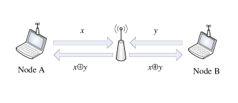
Figure 1: Wireless Switching Network using Network Coding

Packets from node A and B arrive at the relay from two independent Poisson processes with equal parameters $\lambda$ through an ideal channel. We will show that the parameter $\lambda$ could be also applied in renewal process. The relay node maintains two finite buffers to store the backlog packets, which can hold at most $K$ packets, as shown in fig:Queuing-Model-in. The relay employs the following policy in transferring the packet.

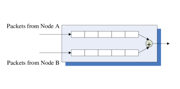
Figure 2: Queuing Model in the Relay Node

1. When a packet arrives, if the queue holding the traffic from the opposite direction is not empty, the relay sends out the coded version of the binary sum of this packet and the packet in the queue from the opposite direction immediately.

2. When a packet arrives, if the queue holding the traffic from the opposite direction is empty, the relay sends out the oldest packet in the queue with the probability of $g_{k}$, where $k$ denotes the current number of storing packet in the queue.

3. When no packet arrives, the relay sends out the packet it stored with a certain probability. This probability is described as a Poisson process depending on the current state $k$. The parameter for this Poisson process is $f_{k}$.

All of above policies are depicted in fig:ENC-Policies. In all cases, we assume that the packet size is small enough that the transmission delay is negligible. In other words, the transmissions can be modeled as points on the time axis. Therefore, the average delay experienced by the packets equals the average amount of time the spend in the queue at the relay. In the next section, we will explore the relationship of the average delay with the average transmission energy of the relay.

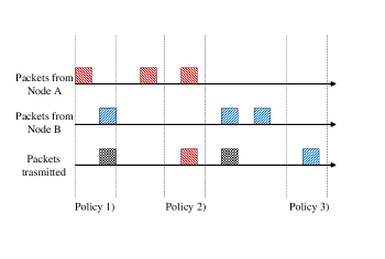
Figure 3: ENC Policies

Note that when the probability of sending an un-coded packet is fixed to be 0, ENC reduces to conventional wireless network coding, where all packets are network-coded. Hence, conventional wireless network coding can be viewed as a special case of ENC. In [8], a policy called “first-come-first-serve”(FCFS) was presented. It can be viewed as another special case of ENC with parameters $f_{k}\equiv 0$. The relay only transmits un-coded packet when buffer is full. There is a brief summary in tab:Policy-comparation-among.

ENC Parameters	$g_{k}$	$f_{k}$
Conventional Network Coding	0	0
“first-come-first-serve”	$g_{k}=\begin{cases}1&k=K\\ 0&k\neq K\end{cases}$	0

TABLE I: Policy comparison among conventional network coding, FCFS and ENC

In this paper, we will show that conventional wireless network coding is not optimal, in terms of delay and packet loss, even results in huge packet-loss rate. The performance limit of wireless network coding, in terms of delay-energy trade-off, will be presented. We shall also optimize ENC to achieve the optimal trade-off.

III Delay-energy Trade-off Analysis

In this section, we present a rigorous mathematical description of ENC. A finite-state Markov chain is formulated for delay and energy consumed analysis.

III-A Why ENC?

Conventional network coding approach usually assumes a buffer with a infinite length on the relay for storing packets. However, in the practical implementation, infinite buffer is impossible. Through the following theorem, we could see that the finite buffer implies the conventional network coding has inevitable packet loss.

First of all, we remark that at most one queue at the relay node can be non-empty. (Otherwise, the relay should XOR and transmit the packets from two queues immediately. We denote the number of packets on the relay at the time instance $t$ by $|R(t)|$, and the number of all packets arriving at the relay before the time instance $t$ by $Q(t)$. If $R(t)>0$, it means that only packets from Node A is in the queue. If $R(t)<0$, packets from Node B can be found in the queue. $B_{k}$ is a random variable represents the $k^{th}$ packets that arriving at the relay. Its definition is as follows:

$$B_{k}:=\begin{cases}1&\text{Packet comes from Node A}\\ -1&\text{Packet comes from Node B}\end{cases}$$

We assume that each $B_{k}$ has independent identical distribution for all $k$ and $E(B_{k}=0$.

Theorem 1

The probability of buffer overflow is

$$\Pr(|R(t)|>K)\approx 2\Phi(-\frac{K}{\sqrt{Q(t)}\sigma_{B}}$$

for any given finite $K$-packet-buffer, where $\sigma_{B}$ is the variance of $B_{k}$, and $\Phi(z)=\Pr(X<z)$, $X\sim N(0,1)$.

Proof:

With the definition in sec:System-Model, since the sum of $B_{k}$ represents the number of remaining packets in the relay, one can easily obtains the following equation,

$$R(t)=\underset{k=1}{\overset{Q(t)}{\sum}}B_{k}$$

When $t\rightarrow\infty$, $Q(t)\rightarrow\infty$, according to central limit theorem, we have

$$R(t)\sim N(0,\sqrt{Q(t)}\sigma_{B}$$

Now let us calculate the probability of buffer overflow.

$$\begin{array}[]{ccc}\Pr(|R(t)|>K)&=&\Pr(|\frac{R(t)}{\sqrt{Q(t)}\sigma_{B}}|>\frac{K}{\sqrt{Q(t)}\sigma_{B}}\\ &\approx&2\Phi(-\frac{K}{\sqrt{Q(t)}\sigma_{B}}\end{array}$$

∎

We know that $\underset{t\rightarrow\infty}{\lim}Q(t)=\infty$. So when $t\rightarrow\infty$, $R(t)$ has infinite variance, and the over flow probability $\Pr(|R(t)|>K)\rightarrow 1$. Thus, without ENC, the system performance will decrease significantly.

This result can also be derived through Little’s Law. Assume that at the time instance $t$, the queue only has the packets from Node A, i.e. $R(t)>0$. At the same time, packets from Node A and Node B arrive at the relay at the identical rate of $\lambda$ packets/second. When packets from Node A arrives, the length of queue increases. We could see that the “arriving rate” is $\lambda$. When packets from Node B arrives, the length of queue decreases with parameter $\lambda$. So the “service rate” is also $\lambda$. According to Little’s Law, a queue with identical arriving time and service time will have infinite length. Thus, with a finite buffer, the packet-loss rate will be unavoidable.

In other case, if Node A and Node B has different flow strength, the situation could be even worse. Assume that the strength of Node A is $\lambda$ and $\mu$ for Node B. If $\lambda>\mu$, in the case above, obviously the “arriving rate” exceeds “service rate”, and the queue will be infinite. If $\lambda<\mu$, when all Node A’s packets are network coded and sent out, Node B’s packets start to accumulate in the queue, which will result in $R(t)<0$, the “arriving rate” exceeds “service rate” again. In the discussion below, we only consider the scenario that Node A and Node B has identical flow strength.

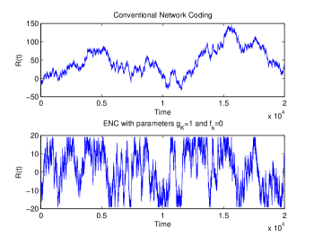
Figure 4: System Performance Comparison between Conventional Network Coding and ENC

fig:System-Performance presents the system performance comparison between conventional network coding and ENC with parameters $g_{K}=1$ and $f_{k}\equiv 0$. The buffer size $K$ is set to 20. In this figure, we can see that in most of time, the buffer overflows in conventional network coding. ENC limits the maximum queue length to be 20. However, this simple group of parameters in not optimal for ENC, since it has potential waste of energy. We will show in the following part of this paper that there exist a group of ENC parameters which fully utilize given energy constraint to achieve minimum delay.

III-B Queuing Model

Before we considering the optimal policy on a finite buffer, we first give a rigorous mathematical model on renewal process queuing and its special case - Poisson process queuing.

III-B1 Renewal Process Queuing Model

A renewal process is a generalization of the Poisson process. In essence, the Poisson process is a continuous-time Markov process on the positive integers which has independent identically distributed holding times at each integer $i$ (exponentially distributed) before advancing to the next integer $i+1$. In a renewal process, the distribution of the gaps has arbitrary independent identical distribution. Let us denote the probability distribution function as $f(t)$ and the total number of packets as $N(t)$.

Definition 1

The short term average renewal rate is defined as

$$\lambda(t):=\frac{dE\left\{N(t)\right\}}{dt}$$

Definition 2

The long term average renewal rate is defined as

$$\lambda^{{}^{\prime}}:=\underset{t\rightarrow\infty}{\lim}\lambda(t)$$

With the above definitions, we notice that $\lambda^{{}^{\prime}}$ has the same character as the parameter $\lambda$ in a Poisson process. It represent the number of packets arriving at the relay in a unit time. In order to calculate $\lambda^{{}^{\prime}}$, we have the following theorems.

Lemma 1

The short term average renewal rate of a renewal process is given by

$$\Lambda(s)=\frac{\psi(s)}{1-\psi(s)}$$

where $\Lambda(s)$ and $\psi(s)$ are Laplace transformation of $\lambda(t)$ and $f(t)$

$$\Lambda(s)=\int_{0}^{\infty}\lambda(t)\exp(-st)dt$$

$$\psi(s)=\int_{0}^{\infty}f(t)\exp(-st)dt$$

Theorem 2

The long term average renewal rate of a renewal process is given by

$$\lambda^{{}^{\prime}}=\frac{1}{\int_{0}^{\infty}tf(t)dt}$$

Proof:

According to def:long-term-average and thm:short-term-average, we have

$$\lambda^{{}^{\prime}} = \underset{t\rightarrow\infty}{\lim}\lambda(t)$$

$$= \underset{s\rightarrow 0}{\lim}s\Lambda(s)$$

$$= \underset{s\rightarrow 0}{\lim}(\frac{s}{1-\psi(s)}-s)$$

$$= \underset{s\rightarrow 0}{\lim}\frac{s}{1-\int_{0}^{\infty}f(t)\exp(-st)dt}$$

$$= \underset{s\rightarrow 0}{\lim}\frac{s}{\int_{0}^{\infty}f(t)stdt}$$

$$= \frac{1}{\int_{0}^{\infty}tf(t)dt}$$

Thus the above theorem holds. ∎

III-B2 Poisson Queuing Model

Let us focus on the special case of renewal process - Poisson process. Assume that the Node A and Node B exchange packets via the relay with the rate of $\lambda$ packet/second, i.e. the short term arriving rate $\lambda(t)$ is a constant. In the following discussion, if we replace the Poisson parameter $\lambda$ with long term average renewal rate $\lambda^{{}^{\prime}}$, all theorems can be applied to renewal process as well.

Based on the transmission policy at the relay described in sec:System-Model, the state of queues at the relay node can be characterized with an integer $S(t)\in[0,K]$, where $K$ represents the total length of queue at the relay.

$$S(t)=|R(t)|$$

Since the future state is independent from its past given the current state, $S(t)$ is a continuous time finite state Markov chain. With the policy defined before, we could derive the transition probability of $S(t)$.

We depict the above mathematical description in fig:Finite-State-Markov.

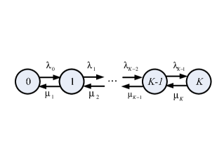
Figure 5: Finite State Markov Chain Model of Buffer State

Theorem 3

The buffer state $S(t)$ is a $K+1$ state Markov Chain with transition probability $\Pr(S(t+\Delta t)=j|S(t)=i)=p_{ij}\Delta t$, which satisfies $p_{ij}=0$ for $|j-i|>1$ and

$$p_{k,k+1}=\begin{cases}\lambda(1-g_{k}&1\leq k\leq K\\ 2\lambda(1-g_{0}&k=0\end{cases}$$ (1)

$$p_{k,k-1}=\lambda+f_{k}$$ (2)

Proof:

First, we derive the transition probability (1) and (2). For $k=0$, the event $S(t+\Delta t)=S(t)+1$ is equivalent to the event that the relay only receives a packet from either source node and does not transmit an un-coded packet. Hence,

$$p_{0,1}=\underset{\Delta t\rightarrow 0}{\lim}\frac{2(\lambda\Delta t)(1-g_{0}}{\Delta t}=2\lambda(1-g_{0}$$

For $1\leq k\leq K-2$, the event $S(t+\Delta t)=S(t)+1$ is equivalent to the event that the relay nodes only receives a packet from the source whose packets are already in the queue, and does not transmit an un-coded packet. Hence, we have

$$p_{k,k+1}=\underset{\Delta t\rightarrow 0}{\lim}\frac{(\lambda\Delta t)(1-g_{k}}{\Delta t}=\lambda(1-g_{k}$$

Note that the event $S(t+\Delta t)=S(t)-1$ is equivalent to the event that (1) the relay only receives a packet from the opposite source to one already in the queue; or (2) the relay transmits an un-coded packet without receiving any packets. As a result,

$$\begin{array}[]{ccc}p_{k,k-1}&=&\underset{\Delta t\rightarrow 0}{\lim}\frac{\lambda\Delta t+[1-2(\lambda\Delta t)](f_{k}\Delta t)}{\Delta t}\\ &=&\lambda+f_{k}\end{array}$$

∎

For convenience, let us denote

$$\lambda_{k}=\begin{cases}p_{k,k+1}&0\leq k\leq K-1\\ \lambda(1-g_{K}&k=K\end{cases}$$ (3)

$$\mu_{k}=p_{k,k-1}$$ (4)

We shall mainly use $\lambda_{k}$ and $\mu_{k}$ rather than $g_{k}$ and $f_{k}$ as the ENC parameters in the following discussion. Also note that $g_{k}\in[0,1]$ and $f_{k}\geq 0$. Thus, $\lambda_{k}$ and $\mu_{k}$ satisfy the following constraints:

$$0\leq\lambda_{k}\leq\begin{cases}2\lambda&k=0\\ \lambda&1\leq k\leq K\end{cases}$$

$$\mu_{k}\geq\lambda$$

III-C Delay and Packet-Loss

With the Markov chain model, we can investigate the network layer performance of ENC, namely, delay and packet-loss. We first present the stationary state probability of $S(t)=k$, denoted by $\pi_{k}$, $k=0,1,\cdots,K$, in the following theorem. The proof of this theorem can be find in [9].

Theorem 4

The stationary state probability $\pi_{k}$ is given by

$$\pi_{k}=\pi_{0}\overset{k-1}{\underset{m=0}{\prod}}\frac{\lambda_{m}}{\mu_{m+1}}$$

where

$$\pi_{0}=[1+\underset{k=1}{\overset{K}{\sum}}\underset{m=0}{\overset{k-1}{\prod}}(\frac{\lambda_{m}}{\mu_{m+1}}]^{-1}$$

We next present the average packet delay by the following corollary, ignoring the potential lost packets.

Corollary 1

The average delay of ENC is given by

$$D=\frac{1}{2\lambda}\underset{k=0}{\overset{K}{\sum}}k\pi_{k}$$

Proof:

Assume that at the time instance $t=t_{0}$, there is $k$ packets in the queue. Let us consider the time a particular packet will experience. Because ENC policy means no difference between two nodes, the probability that this $k$ packets has the same source origin as our last packet is $\frac{1}{2}$. Thus the average length of the queue consisting of the packets from a particular node can be obtained as

$$\bar{K}=\frac{1}{2}\underset{k=0}{\overset{K}{\sum}}k\pi_{k}$$

Recall that the average arriving time of a Poisson process is $\lambda$, according to the Little’s law, (1) holds. ∎

We can also characterize the packet-loss rate of ENC.

Corollary 2

The normalized packet-loss rate of ENC is given by

$$\xi=\frac{\pi_{K}\lambda_{K}}{2\lambda}$$

Proof:

As mentioned above, the packet loss of ENC results from a full queue. The buffer overflow event is equivalent as follows:

$$\Pr(S(t+\Delta t)>K)=\Pr(S(t)=K)\lambda_{K}\Delta t$$

This is the buffer overflow probability for a single packet. We should normalize it by dividing it with the total number of packets that arrives at the relay in the time interval $\Delta t$, i.e. $2\lambda\Delta t$. Thus, the corollary is verified. ∎

To avoid retransmission, packet dropping is not allowed in the relay node. As a result, when the buffer is in state $S(t)=K$, the relay must send a packet if it receives a packet from the source whose packets are already in the queue. Thus, we have $g_{K}=1$, or equivalently,

$$\lambda_{K}=0$$

In particular, as shown in sub:Why-do-we, conventional wireless networking’s packet-loss rate cannot be 0 in general. However, in some scenario, such as UDP, packet loss is allowed. We will see that allowing $\xi\neq 0$ further reduce the energy needed.

III-D Energy Consumption

Having obtained the delay and packet-loss rate of ENC, we now focus on its energy consumption. As described in sec:System-Model, the relay transmits a packet under any of three circumstances. Thus, we have the following theorem:

Theorem 5

Conditioned on the buffer state $S(t)=k$, the energy consumption $\varepsilon_{k}$ is a random variable satisfying

$$\Pr(\varepsilon_{k}=\varepsilon|S(t)=k)=\begin{cases}-\lambda_{0}+2\lambda&k=0\\ -\lambda_{k}+\mu_{k}+\lambda&1\leq k\leq K\end{cases}$$ (5)

$$\Pr(\varepsilon_{k}=0|S(t)=k)=1-\Pr(\varepsilon_{k}=\varepsilon|S(t)=k)$$ (6)

where $\varepsilon$ is the average energy for transmitting one packet.

Proof:

For $k=0$, the relay transmits with probability $g_{0}$ when receiving packet from either source.

$$\varepsilon_{0}=\varepsilon\underset{\Delta t\rightarrow 0}{\lim}\frac{2(\lambda\Delta t)g_{0}}{\Delta t}=2\lambda g_{0}\varepsilon=\varepsilon(-\lambda_{0}+2\lambda)$$

For $1\leq k\leq K$, the relay transmits when (1) receiving a packet from opposite source; (2) receiving a packet from the same source whose packets are already in queue (with probability $g_{k}$); (3) receiving no packet and transmitting the oldest packet in queue.

$$\begin{array}[]{ccc}\varepsilon_{k}&=\varepsilon&\underset{\Delta t\rightarrow 0}{\lim}\frac{(\lambda\Delta t)(1+g_{k}+(1-2\lambda\Delta t)(f_{k}\Delta t)}{\Delta t}\\ &=&\varepsilon[\lambda(1+g_{k}+f_{k}]\\ &=&\varepsilon(-\lambda_{k}+\mu_{k}+\lambda)\end{array}$$

Hence, (5) holds. (6) can then be verified by the probability normalization ∎

The average energy consumed in the relay node can be given by the following theorem.

Theorem 6

With ENC, the average energy consumed in the relay node can be given by

$$E^{ave}=\varepsilon(\lambda\pi_{0}+\lambda-\lambda_{K}\pi_{K}$$ (7)

Proof:

According to the definition of the average energy,

$$E^{ave}=\underset{k=0}{\overset{K}{\sum}}\varepsilon_{k}\pi_{k}$$ (8)

Then by substituting (5) into (8), it follows that

$$\begin{array}[]{ccc}E^{ave}&=&\varepsilon[(-\lambda_{0}+2\lambda)\pi_{0}+\underset{k=1}{\overset{K}{\sum}}(-\lambda_{k}+\mu_{k}+\lambda)\pi_{k}]\\ &=&\varepsilon[\lambda\pi_{0}+\lambda-\underset{k=0}{\overset{K-1}{\sum}}\lambda_{k}\pi_{k}+\underset{k=1}{\overset{K}{\sum}}\mu_{k}\pi_{k}-\lambda_{K}\pi_{K}]\end{array}$$ (9)

According to the character of stationary probability,

$$\underset{k=0}{\overset{K-1}{\sum}}\lambda_{k}\pi_{k}=\underset{k=1}{\overset{K}{\sum}}\mu_{k}\pi_{k}$$

Then by substituting (III-D) into (9), (7) holds. ∎

For different physical layer designs, the transmission energy $\varepsilon$ can be different. And for different data rate, $\lambda$ is different as well. We notice that $E^{ave}$ is a linear function of $\varepsilon\lambda$. To obtain a unified result, we divide $E^{ave}$ with $\varepsilon\lambda$

$$\overline{E}=\frac{E^{ave}}{\varepsilon\lambda}=\pi_{0}+1-2\xi$$

We notice that when the packet-loss rate is 0 for ENC, namely, $\xi=0$, the normalized average energy can be further simplified to be

$$\overline{E}=\pi_{0}+1$$

The normalized energy $\overline{E}$ represents the ratio of the actual energy $E^{ave}$ to the average arriving rate $\lambda$ and the average one-time energy consumption $\varepsilon$. According to (4), the performance of ENC is determined by the transition probabilities $\lambda_{k}$ and $\mu_{k}$. A key problem for ENC is, therefore, how to choose $\lambda_{k}$ and $\mu_{k}$ to optimize the system performance in terms of delay and energy.

IV Optimal Delay-energy Trade-off

We have already related the performance of ENC, in terms of average delay and energy consumption, to the transition probabilities $\lambda_{k}$ and $\mu_{k}$, in sec:Energy-Delay-Trade-off-Analysis. In this section, we shall address the fundamental problem of how can the average delay of ENC be minimized given an average energy constraint. The discussion is conducted in two parts - loss-free and non-loss-free.

IV-A Loss-free Scenario

Let $\bar{E}^{max}$ denote the normalized energy constraint. In this context, a deterministic optimization problem for minimizing the packet delay, $D$, of ENC can be formulated as follows.

Problem 1

Minimize $D=\frac{1}{2\lambda}\underset{k=0}{\overset{K}{\sum}}k\pi_{k}$, subject to

$$\begin{cases}\pi_{0}+1\leq\bar{E}^{max}\\ 0\leq\lambda_{k}\leq\begin{cases}2\lambda&k=0\\ \lambda&1\leq k\leq K\end{cases}\\ \mu_{k}\geq\lambda\\ \pi_{k}=\pi_{0}\overset{k-1}{\underset{m=0}{\prod}}\frac{\lambda_{m}}{\mu_{m+1}}\\ \pi_{0}=[1+\underset{k=1}{\overset{K}{\sum}}\underset{m=0}{\overset{k-1}{\prod}}(\frac{\lambda_{m}}{\mu_{m+1}}]^{-1}\end{cases}$$

Let $D^{*}$ denote the minimal delay determined by the above problem. Intuitively, $D^{*}$ is a decreasing function of $\bar{E}^{max}$,which we shall denote as

$$D^{*}=d^{*}(\bar{E}^{max}$$

The function $d^{*}(\centerdot)$ represents the optimal delay-energy trade-off. In this paper, we are interested in both the formulation of the trade-off function and how to achieve the optimal trade-off. To do this, we convert pro:Minimize into a linear programming problem as described in the following theorem.

Theorem 7

The optimization pro:Minimize is equivalent to a linear programming problem given by

Minimize $D=\frac{1}{2\lambda}\pi_{0}^{*}\underset{k=1}{\overset{K}{\sum}}k\rho_{k}$, subject to

$$\begin{cases}\underset{k=1}{\overset{K}{\sum}}\rho_{k}=\frac{1}{\pi_{0}^{*}}-1\\ \rho_{1}\leq 2\\ \rho_{k+1}-\rho_{k}\leq 0&1\leq k\leq K-1\\ \rho_{k}\geq 0\end{cases}$$

where $\pi_{0}^{*}$ is a constant defined by the following formula.

$$\pi_{0}^{*}=\begin{cases}0&\bar{E}^{max}<1\\ \bar{E}^{max}-1&1\leq\bar{E}^{max}\leq 2\\ 1&\bar{E}^{max}>1\end{cases}$$

Proof:

Let

$$\rho_{k}=\overset{k-1}{\underset{m=0}{\prod}}\frac{\lambda_{m}}{\mu_{m+1}}$$

It is easily seen that $\rho_{k}\geq 0$. Also, we have

$$\rho_{1}=\frac{\lambda_{0}}{\mu_{1}}\leq 2$$

Since

$$\rho_{k+1}=\frac{\lambda_{k}}{\mu_{k+1}}\rho_{k}$$

We get $\rho_{k+1}-\rho_{k}\leq 0$.

Next, we note that the average delay is decreased with the increase of the average energy. To achieve the maximum energy allowed, we could make $\pi_{0}$ to be

$$\pi_{0}=\bar{E}^{max}-1$$

At the same time, also note that $\pi_{0}\leq 1$. Thus,

$$\pi_{0}^{*}=\begin{cases}0&\bar{E}^{max}<1\\ \bar{E}^{max}-1&1\leq\bar{E}^{max}\leq 2\\ 1&\bar{E}^{max}>2\end{cases}$$

Then the above theorem follows. ∎

Next, we present the analytical optimal solution to thm:The-optimization-Problem.

Theorem 8

The analytical optimal solution to thm:The-optimization-Problem is given by

$$\rho_{k}^{*}=\begin{cases}2&k\leq k^{*}\\ \frac{1}{\pi_{0}^{*}}-1-2k^{*}&k=k^{*}+1\\ 0&k>k^{*}+1\end{cases}$$ (10)

where

$$k^{*}=\left\lfloor(\frac{1}{\pi_{0}^{*}}-1)/2\right\rfloor$$ (11)

Proof:

Note that the objective function is the weighted summation of $\rho_{k}$ with weight $k$. Subject to the given summation of $\rho_{k}$, one needs to minimize the $\rho_{k}$ with a relatively larger weight to minimize the weighted summation. As a result, there exists a positive integer $k^{*}$, which satisfies

$$0=\rho_{K}^{*}=\cdots=\rho_{k^{*}+2}^{*}\leq\rho_{k^{*}+1}^{*}<\rho_{k^{*}}^{*}=\cdots\rho_{1}^{*}=2$$

According to the constraint, $k^{*}$ is the largest integer satisfying

$$2k^{*}\leq\frac{1}{\pi_{0}^{*}}-1$$

So the theorem holds. ∎

Having solved the linear programming problem, we next present the optimal delay-energy trade-off function as well as the optimal ENC that can achieve that trade-off.

Theorem 9

The optimal ENC delay-energy trade-off function for loss-free transmission is

$$\begin{array}[]{l}d=\\ \begin{cases}\frac{k^{*}+1}{2\lambda}[1-(\bar{E}^{max}-1)(k^{*}+1)]&\frac{1}{1+2K}+1\leq\bar{E}^{max}\leq 2\\ 0&\bar{E}^{max}>2\end{cases}\end{array}$$ (12)

Proof:

Notice that the maximum length of queue is $K$. We have

$$\underset{k=1}{\overset{K}{\sum}}\rho_{k}\leq 2K$$

Thus,

$$\bar{E}^{max}\geq 1+\frac{1}{1+2K}$$ (13)

Otherwise, the feasible region is empty and hence there is no solution. Next, we substitute (11), (10) into equations in thm:The-optimization-Problem, the above theorem holds. ∎

According to thm:The-optimization-Problem, we can also present the optimal parameters for ENC.

Theorem 10

One group of optimal parameters for ENC with maximal average energy $\bar{E}^{max}$ are given as follows:

$$\lambda_{k}^{*}=\begin{cases}2\lambda&k=0\\ \lambda&1\leq k\leq k^{*}\\ 0&k^{*}+1\leq k\leq K\end{cases}$$ (14)

$$\mu_{k}^{*}=\begin{cases}\lambda&k\neq k^{*}+1\\ \frac{2\lambda}{\rho_{k^{*}+1}^{*}}&k=k^{*}+1\end{cases}$$ (15)

Proof:

From (IV-A), (IV-A), and (10), we have $\lambda_{0}^{*}=2\mu_{1}^{*}$, and $\lambda_{k}^{*}=\mu_{k+1}^{*}$ for $k\leq k^{*}$. For $k>k^{*}+1$, $\rho_{k}^{*}=0$, thus $\lambda_{k-1}^{*}=0$ and $\mu_{k}^{*}$ can be any positive value. We let $\mu_{k}^{*}=\lambda$ for convenience. Finally, note that $\rho_{k^{*}}^{*}=2$, thus $\mu_{k^{*}+1}^{*}=\frac{2\lambda}{\rho_{k^{*}+1}^{*}}$. ∎

By substituting (14), (15) into (3), (4), we can obtain the optimal probability of transmitting a packet without network coding

$$g_{k}^{*}=\begin{cases}0&k\leq k^{*}\\ 1&k^{*}+1\leq k\leq K\end{cases}$$ (16)

$$f_{k}^{*}=\begin{cases}\frac{2\lambda}{\rho_{k^{*}+1}^{*}}-\lambda&k=k^{*}+1\\ 0&k\neq k^{*}+1\end{cases}$$ (17)

This is the analytical result of delay-energy trade-off curve lower bound. ENC on this parameters could achieve the delay lower bound given energy constraint.

IV-B Non-loss-free Scenario

In this subsection, the optimal delay function and ENC parameters that satisfy the allowed normalized packet loss rate $\xi$ are presented. We assume that the packet-loss in ENC only is only introduced by a full queue. Note that the delay in non-loss-free scenario only represents the delay of the packets that arrive at the destination successfully.

Theorem 11

The optimal delay-energy trade-off function that achieve normalized packet loss rate $\xi$ in a $K$-packet buffer is

$$d=\frac{K}{2\lambda}[1-(\bar{E}^{max}-1+2\xi)K]$$ (18)

where $\frac{1}{1+2K}+1-2\xi\leq\bar{E}^{max}\leq\frac{1}{1+2K}+1$.

Proof:

Recall that in (13), we require that $\bar{E}^{max}\geq 1+\frac{1}{1+2K}$. However, this constraint is not always satisfied. (III-D) implies that the normalized packet loss rate $\xi$ can be view as a virtual energy that lowers down the energy threshold from $1+\frac{1}{1+2K}$ to $1+\frac{1}{1+2K}-2\xi$. Moreover, in this case, from (10), $\rho_{K}=\frac{1}{\pi_{0}}-1-2(K-1)=2$. Thus, $k^{*}+1=K$ according to (11). The optimal delay function can be applied to non-loss-free scenario simply by replacing $\bar{E}^{max}$ with $\bar{E}^{max}+2\xi$ in (12) and replacing $k^{*}+1$ with $K$. ∎

In the non-loss-free scenario, we are not interested system performance in terms of delay and energy. We are more interested in how to configure ENC’s parameters - especially $g_{k}$ to achieve particular packet loss rate.

Theorem 12

The parameters of ENC that achieve normalized packet loss rate $\xi$ in a $K$-packet buffer with energy constraint $\bar{E}^{max}=1+\frac{1}{1+2K}-2\xi$ is

$$g_{k}=\begin{cases}1&0\leq k\leq K-1\\ 1-(1+2K)\xi&k=K\end{cases}$$

$$f_{k}\equiv 0$$

Proof:

According to (III-D),

$$\pi_{0}=\bar{E}^{max}-1+\xi=\frac{1}{1+2K}$$

As we already know in the proof to the last theorem, $\rho_{K}=2$, we have $\pi_{K}=\pi_{0}\rho_{K}=\frac{2}{1+2K}$. Recall the definition of normalized packet loss rate,

$$\pi_{K}\lambda_{K}=2\xi\lambda$$

By substitute (IV-B) into (3), the theorem holds. ∎

fig:Packet-loss-Rate shows the relationship between normalized packet loss rate $\xi$ and ENC parameter $g_{K}$. We could see that $g_{K}$ changes linearly against $\xi$. However, one can not save energy in exchange of packet loss rate unlimitedly. It is because the stationary probability of a full queue $\pi_{K}$ is not large enough for introducing a packet loss rate of $\xi$. When $\xi$ exceeds $\frac{1}{1+2K}$, i.e. the normalized energy constraint is less than $1-\frac{1}{1+2K}$, ENC can not achieve the minimal energy constraint by enhancing allowed packet loss rate constraint.

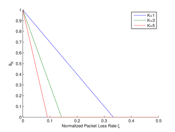
Figure 6: Packet-loss Rate of ENC

V Numerical Results

In this section, sample numerical results are presented to demonstrate the potential of ENC and validate the theoretical results of this work. We developed a event-driven simulator with C++ based on Monte-Carlo method to verify our theoretical model.

V-A Packet Loss Rate for Conventional Network Coding

In (12), if we let $g_{K}=0$, the ENC reduces to conventional network coding. We are interested in acquiring the curve of normalized packet-loss rate $\xi$ against the buffer length $K$ when $g_{K}=0$. fig:Conventional-Packet-Loss presents the theoretical curve of $\xi=\frac{1}{1+2K}$ and simulation result in squares.

Figure 7: Packet Loss Rate for Conventional Network Coding

Again, we observe that with a finite buffer, conventional network coding will result in inevitable packet loss, i.e. $\xi\neq 0$. However, when conventional network coding scheme employs a larger buffer, the packet loss rate will decreases.

V-B Delay-Energy Trade-off for ENC

Assume that the maximal relay buffer space is $K=3$. The theoretical optimal delay-energy trade-off curve, as well as the simulation results of the optimal trade-off achieving ENC strategies, is presented.

We observe the delay and energy consumed while changing $f_{k}^{*}$ and $k^{*}$. fig:Optimal-Delay-Power-Trade-off shows the theoretical and simulation results for the optimal delay-energy trade-off. The theoretical optimal trade-off curve is shown by the solid line. The simulation results for the four optimal ENC strategies are show by the squares in the three cases. It can be seen that the simulation results fit on the theoretical curve perfectly.

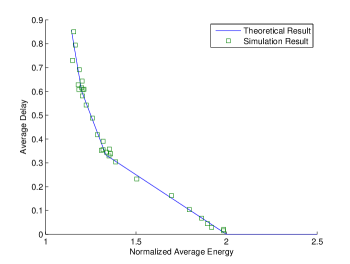
Figure 8: Optimal Delay-energy Trade-off for ENC

From this result, we could see that

1. The optimal delay is a decreasing function of minimal energy constraint. The curve consists $K$ straight lines, which indicates the delay is linear to the minimal energy constraint.

2. In the simulation, notice the three special cases, where the energy constraints are given by

   $$\begin{array}[]{cc}\bar{E}_{m}^{max}=1+\frac{1}{1+2m}+\delta&m=1,2,3\end{array}$$

   where $\delta\rightarrow 0^{+}$. Recall that in (10), (16) and (17),

   $$\rho_{k^{*}+1}^{*}=\frac{1}{\pi_{0}^{*}}-1-2\left\lfloor(\frac{1}{\pi_{0}^{*}}-1)/2\right\rfloor\in[0,2]$$

   When $\bar{E}_{m}^{max}$ is slightly larger than $1+\frac{1}{1+2m}$, $\rho_{k^{*}+1}^{*}=2$, $f_{k^{*}+1}^{*}=0$. So we have $k^{*}+1=m$ and $f_{k}^{*}\equiv 0$ for any $k$ in this case. The optimal ENC strategy becomes quite simple.

3. When the energy constraint is large, namely, $\bar{E}^{max}>2$, the delay is zero. That means the relay transmits a packet the time receiving it without storing. When the energy constraint is small, the delay increases rapidly. When $\bar{E}^{max}<1+\frac{1}{1+2K}=1+\frac{1}{7}\approx 1.143$, the delay is infinite, which indicates the given energy is not sufficient for packet-loss free transmitting. Recall that in sub:Why-do-we, we prove that conventional network coding could not avoid packet loss in a finite buffer. Here we can easily see that the conventional network coding has the normalized energy constraint $\bar{E}^{max}=1<1+\frac{1}{1+2K}$ for any positive integer $K$.

VI Conclusions

In this paper, we proposed a continuous-time opportunistic network coding or ENC method in the continuous time domain, where the relay node can transmit either network-coded or un-coded packets. We show that the conventional network coding scheme on a finite buffer implies inevitable packet loss. By using a Markov model, the packet delay, packet-loss rate, and average energy consumption of ENC were presented for general renewal process queuing and classical Poisson process queuing. Given the delay and energy results, the performance bound of ENC was proposed in terms of delay-energy trade-off. We also presented an ENC strategy which can achieve the optimal trade-off. Through simulations, the developed theoretical results were validated. It was also demonstrated that the proposed ENC can achieve lower delay compared to conventional wireless network coding scheme.

References

- [1] W. Chen, K. Letaief, and Z. Cao, “Opportunistic network coding for wireless networks,” in Communications, 2007. ICC ’07. IEEE International Conference on, 2007, pp. 4634–4639.
- [2] R. Ahlswede, N. Cai, S.-Y. Li, and R. Yeung, “Network information flow,” Information Theory, IEEE Transactions on, vol. 46, no. 4, pp. 1204–1216, 2000.
- [3] P. A. C. Wu and S.-Y. Kung, “Information exchange in wireless networks with network coding and physical layer-broadcast,” Microsoft Research, Tech. Rep. MSR-TR-2004-78, 8 2004.
- [4] W. Chen, K. Letaief, and Z. Cao, “A cross layer method for interference cancellation and network coding in wireless networks,” in Communications, 2006. ICC ’06. IEEE International Conference on, vol. 8, 2006, pp. 3693–3698.
- [5] ——, “Wlc46-6: Cooperative interference cancellation in multi-hop wireless networks: A cross layer approach,” in Global Telecommunications Conference, 2006. GLOBECOM ’06. IEEE, 2006, pp. 1–5.
- [6] P. Popovski and H. Yomo, “Bi-directional amplification of throughput in a wireless multi-hop network,” in Vehicular Technology Conference, 2006. VTC 2006-Spring. IEEE 63rd, vol. 2, 2006, pp. 588–593.
- [7] S. Zhang, S. chang Liew, and P. P. Lam, “Physical-layer network coding,” in in ACM Mobicom ‘06, 2006.
- [8] X. He and A. Yener, “On the energy-delay trade-off of a two-way relay network,” in Information Sciences and Systems, 2008. CISS 2008. 42nd Annual Conference on, 2008, pp. 865–870.
- [9] L. Kleinrock, Queuing Systems, Volume I: Theory. Wiley-Interscience, 1975.