Reversible first-order transition in Pauli percolation

Abstract

Percolation plays an important role in fields and phenomena as diverse as the study of social networks, the dynamics of epidemics, the robustness of electricity grids, conduction in disordered media, and geometric properties in statistical physics. We analyse a new percolation problem in which the first order nature of an equilibrium percolation transition can be established analytically and verified numerically. The rules for this site percolation model are physical and very simple, requiring only the introduction of a weight $W(n)=n+1$ for a cluster of size $n$. This establishes that a discontinuous percolation transition can occur with qualitatively more local interactions than in all currently considered examples of explosive percolation; and that, unlike these, it can be reversible. This greatly extends both the applicability of such percolation models in principle, and their reach in practice.

Introduction. The percolation transition involves fundamentally geometric properties, manifest in non-local observables such as an onset of conductivity in a dirty metal, a breakdown of an electrical grid or an epidemic disease outbreak Isichenko1992; Stauffer1994; Moore200epidemics; Golnoosh2012. This is at odds with the more standard phase transitions in statistical physics which are described by a local order parameter, such as the magnetisation in a bar magnet. It thus involves a conceptually fundamentally distinct set of issues. Its wide applicability coupled with this fundamental importance have generated much interest in defining various types of percolation problems and analysing their concomitant phase transitions. One enterprise has been the quest for a first-order percolation transition, where the percolating cluster sets in discontinuously, corresponding to a particularly violent transition, which can qualitatively amplify desirable properties in applications. Such a transition has remained remarkably elusive, but the development which has taken place under the heading of explosive percolation has finally yielded one, via a mechanism in which an infinite number of nonlocal interactions need to occur simultaneously Achlioptas2009; daCosta2010; Riordan2011; Ziff2009; Pan2011; Grassberger2011; Panagiotou2013; Manna2010; Cho2013.

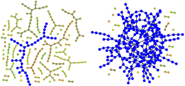
Here, we study Pauli percolation – a site percolation problem with its origin in correlated quantum magnetism, characterized by a number of novel striking and desirable properties. First of all, it exhibits a first-order phase transition invoking only a minimal amount of non-locality, in the form of an interaction solely between adjacent clusters, depending only on their respective sizes. Secondly, such an interaction can be very easily generated from perfectly local ones, for instance either via a simple classical colouring rule, or via a quantum-statistical interaction between Fermionic particles. Thirdly, it describes an equilibrium phase transition, and is hence reversible; at the same time, it can be thought of and analysed as a stochastic dynamical process and thus may – but need not – exhibit hysteresis. Finally, Pauli percolation lends itself to investigations using the toolbox of equilibrium classical statistical mechanics; we are thus able to solve its properties analytically on a regular random graph, and verify this solution via numerical Monte Carlo simulations.

Pauli percolation.

Figure 1: (a) In Pauli percolation, weight ${W=n+1}$ of a cluster can be reproduced by imposing a simple two-color ‘contagion’ rule shown here: the whole cluster of occupied sites can be either healthy (green) or have a single infected site (red). Different cluster configurations appear with different statistical weights. (b) The explosive nature of a Pauli-percolation transition on a regular random graph of $N=400$ sites: two representative configurations, without and with a giant cluster at the same site fugacity corresponding to $\tilde{p}=0.45$ are shown side by side. The largest cluster is colored blue; unoccupied sites are not shown.

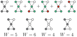
The model we consider first arose in a quantum many-body problem of itinerant electrons on lattices with flat energy bands. Such a system can exhibit flat-band ferromagnetism: the Pauli exclusion principle mandates that in the ground state the electron spins in a cluster order ferromagnetically in order to minimize the energy of repulsive on-site interactions Mielke1993. This leads to a weight of $(n+1)$, reflecting the number of possible orientations of the total spin of a ferromagnetic cluster of $n$ electrons Maksymenko2012.

The corresponding statistical-mechanical problem describes $M$ particles occupying random sites of a lattice. Every configuration $\mathcal{C}=\cup_{i}\mathcal{C}_{i}$ appears with statistical weight $W_{\mathcal{C}}=\prod_{i}(n(\mathcal{C}_{i})+1)$, with $n(\mathcal{C}_{i})$ being the size of cluster $\mathcal{C}_{i}$. The partition function is therefore $Z=\sum_{\{\mathcal{C}\}}W_{\mathcal{C}}.$

Merging two clusters of size $m$ and $n$ reduces their overall weight from $(m+1)(n+1)$ to $(m+n+1)$ – a dramatic reduction for large clusters resulting in an effective repulsive interaction between them. This is reminiscent of the ‘product rule’ leading to explosive percolation suggested by Achlioptas Achlioptas2009 and developed in Manna2010; Cho2013; Ziff2013 but there are fundamental differences, see discussion below.

Rather then fixing the number of occupied sites, we can study the grand canonical ensemble by letting each site of the lattice be occupied with an a priori probability ${p}$ or left empty with an a priori probability $1-{p}$. The grand canonical partition function is then

$$Z=\sum_{\{\mathcal{C}\}}\left(\frac{p}{1-p}\right)^{n(\mathcal{C})}W_{\cal C}$$ (1)

where $\ln{\left[{p}/(1-{p})\right]}$ plays the role of a chemical potential controlling the density of occupied sites and letting it fluctuate. Note that a priori probability ${p}$, unlike a regular site percolation, is not equal to the density of occupied sites.

This model also has a simple representation as a particular classical two-color, or contagion, percolation problem. It is a mild variation of regular percolation: sites can come in two colors, green (uninfected) or red (infected). Specifically, each site of a lattice is occupied and colored either green or red with an a priori probability $\tilde{p}$ each, or left empty with an a priori probability $1-2\tilde{p}$. Only configurations $\{{\mathcal{G}}\}$ where every cluster contains no more than one red site are taken into account. The partition function of this model is then simply

$$Z_{\text{gr}}\!=\!\sum_{{\{{\mathcal{G}}}\}}\left(\frac{\tilde{p}}{1-2\tilde{p}}\right)^{n({\mathcal{G}})}$$ (2)

It is straightforward to see that tracing over all possible site colors consistent with fixed site occupations renders Eq. (2) identical to Eq. (1) (with the identification of $\tilde{p}=p/(p+1)$): each cluster may have either all sites green (uninfected), or at most one red (infected) site. Therefore a cluster of $n$ sites has weight ${(n+1)}$ after the sum over possible locations of red sites is taken into account. The utility of the formulation as a two-color percolation problem lies in the fact that the need ever to compute cluster sizes is obviated: the choice of location of the infected site takes care of that.

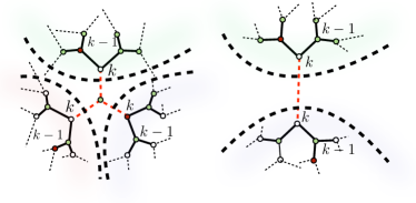
Analytic and numerical results. We show that Pauli percolation exhibits a discontinuous percolation transition in infinite dimensions by studying it analytically and numerically on a regular random graph of ${N}$ sites. Such graphs are often used to approximate random networks Dorogovtsev2010book. They have a vanishing density of short cycles and mostly contain loops of size $\ln{N}$; hence they are locally tree-like Mezard2001; Janson2000. This property enables us to develop an exact solution via a so-called cavity method widely used in spin glass and optimization problems Mezard2001; Laumann2008; Rivoire2005; Barre2007; Hsu2013. In the cavity method, adding a site or an edge to a $z$-regular random graph is equivalent to connecting $z$ or $z-1$ roots (here referred to as cavity sites) of independent Cayley trees (see Figure 2) via that site or edge. To complete the correspondence and get the correct set of solutions we introduce ‘wired’ boundary conditions which connect the outer sites (‘leaves’) with one another thus allowing the formation of loops.

The recursive structure of calculations on Cayley trees makes the mean-field treatment exact in these systems. Care must be taken to correctly calculate the bulk thermodynamic potentials on such structures Hoory2006; Laumann2009; Barre2007; Barre2001. For instance, the bulk free energy is computed as a change in free energy due to the addition of a site and the corresponding links emanating from this site ${\mathcal{F}=\lim_{k\to\infty}\left[-\ln{{\mathcal{Z}}/Z_{k}^{3}}+\left(z/2\right)\ln{{\tilde{\mathcal{Z}}}/Z_{k}^{2}}\right]}$, where ${\mathcal{Z}}$ and $\tilde{\mathcal{Z}}$ are the partition functions for a uniform Bethe lattice obtained by connecting either $z$ or $z-1$ root sites of independent trees via a new site or edge. $Z_{k}$ is the partition function for a level-$k$ tree Mezard2001; Laumann2008; Rivoire2005; Barre2007; Hsu2013.

Figure 2: (a) Properties of a regular random graph make it locally equivalent to the neighborhood of an internal site of a Bethe lattice obtained by connecting roots of independent Cayley trees via site or edge addition. Here the sites colors (red/dark grey and green/light grey) represent one instance allowed by the two-color contagion percolation rules. (b) The upper pane shows the probability ${\mathcal{P}}_{\infty}$ that a site belongs to a giant cluster as a function of $\tilde{p}$. The blue diamond marks $\tilde{p}=4/9$ at which the nonzero solution appears. The lower pane shows the ‘bulk’ free energy per site of a 3-regular random graph corresponding to each of these solutions (see text for details). The red pentagon indicates the transition point. Bold parts of the lines in both panels indicate the actual solution.

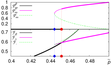
In the first instance we are interested in the existence of a giant cluster (i.e. a cluster occupying a finite fraction of the lattice), in the simplest case of $z=3$. We define ${\mathcal{P}}_{\infty}$ to be the probability that a given site belongs to such giant cluster; see Supplementary Material for details. For $\tilde{p}<4/9$, the only solution of the resulting equations is ${\mathcal{P}}^{\text{0}}_{\infty}=0$ – in other words, there is no percolation. For $\tilde{p}\geq 4/9$ two more solutions appear with ${\mathcal{P}}^{\pm}_{\infty}\neq 0$ as shown in Figure 2 (with the lower brunch being unphysical) . Note that there is never a percolating uninfected cluster: the probability that a given cluster of size $n$ remains uninfected is $1/(n+1)$.

The topology of the plot for ${\mathcal{P}}_{\infty}$ already demonstrates the first order nature of the percolation transition: the curve which yields the solution $\mathcal{P}^{+}_{\infty}=1$ (i.e. all sites are occupied) for $\tilde{p}\to 1/2$ never crosses the non-percolating solution $\mathcal{P}^{\text{0}}_{\infty}=0$, which in turn is unique for $\tilde{p}\to 0$. The transition from one to the other therefore implies a jump in $\mathcal{P}_{\infty}$! To determine when the actual transition takes place we analyze the bulk free energy of the problem. The solution which minimizes this quantity maximizes the partition function and thus is selected. This selects the solution of ${\mathcal{P}}^{+}_{\infty}\neq 0$ at $\tilde{p}_{c}=0.451606...$(See Figure 2) indicating a discontinuous jump as soon as $\tilde{p}=\tilde{p}_{c}$. We note that this is in agreement with other quantities such as cluster size distribution and average cluster size which show no signature of power-law distribution or divergence at the transition point. These, together with details of the computation, are shown in the Supplemental Material.

Figure 3: (a) Density $\rho$ versus a priori probability $\tilde{p}$. Red line indicates the exact solution while the dots represent Monte-Carlo results for 3-regular random graphs of sizes ${N}=50,100,200,300,400,600,800$. (b) Finite size extrapolation of the minimum of the fourth-order Binder cumulant of density $\cal{U}$ and point of equally weighed peaks of histograms of density $P(\rho)$. The red pentagon marks the point at which the infinite cluster appears in the thermodynamic limit, at a density distinct from where the solutions ${\cal P}^{\pm}_{\infty}$ first appear, indicated by the blue diamond.

We support our analytic results by Monte-Carlo simulations of Eq. (1) on a regular random graph. We analyze density of occupied sites $\rho$ as well as histograms of its distribution along with the fourth-order Binder cumulant $\mathcal{U}$ as standard indicators of phase transitions. In all the quantities the extrapolation to ${N}\rightarrow\infty$ is consistent with the exact solution. Below and above the transition the numerical data follows the branches of the exact solution for the uniform Bethe lattice. The histograms of the density distribution give a clear double peak structure – the hallmark of a discontinuous transition – and in Figure 3 we provide an extrapolation of the point at which these two peaks are of equal weight. This nicely extrapolates to the analytic result for the transition point $\tilde{p}_{c}=0.452(3)$. Finally the density Binder cumulant $\mathcal{U}$ develops a minimum at the transition point – a typical behavior for a discontinuous transition; its extrapolation to thermodynamic limit is also in good agreement with the transition point obtained analytically.

Discussion. The attractiveness of Pauli percolation is manifold. Firstly, it is underpinned by a simple and transparent physical mechanisms. Secondly, it is amenable to detailed numerical and analytical analyses. Thirdly, and crucially, it exhibits a remarkable phenomenology featuring a reversible first-order percolation transition. In the following, we discuss the import of these items, and embed them in a broader zoology of percolation problems.

The notion of explosive first-order percolation Achlioptas2009 has been met with much excitement, yet the initial approach proved to be deficient Riordan2011. A discontinuous transition has finally been found in several variants of explosive percolation models which, however, require a very elevated degree of non-locality: a dynamical process defining these models involves a comparison between an extensive number of degrees of freedom before a configuration change occurs daCosta2010; Riordan2011; Grassberger2011; Manna2010. Recent studies also considered suppressing the onset of percolation through a rule explicitly inhibiting bond addition if it leads to the formation of a spanning cluster Cho2013. Not only such a process involves an extensive number of local degrees of freedom, it also makes the ‘microscopic’ dynamics of the model – a placement of a particular bond – explicitly depend on the onset of a global phenomenon, percolation.

Pauli percolation, by contrast, considers one site at a time, with a minimal amount of non-locality entering only via the sizes of the clusters impinging on the site in question. In other words, Pauli percolation is non-local only up to the size of the clusters present locally. The Pauli principle of quantum mechanics presents a straightforward physical origin for such a weight: quantum statistical interactions are intrinsically non-local on this level. A classical route to the same weights involves permitting at most one site of each cluster to be infected, again a simple and intuitive description involving clusters only locally and individually.

Nor does Pauli percolation require the irreversibility of explosive percolation. Based on statistical weights of configurations rather than rules for cluster growth, Pauli percolation provides an equilibrium first-order transition. It in particular allows for shrinking, as well as growing, clusters. It therefore naturally accommodates healing/repairing processes, in e.g. network applications which, notably, can remove percolation discontinuously. The growth process encoded by the “product rule” in explosive percolation is reminiscent of the weights of Pauli percolation: the latter, however, provides a natural prescription for removing particles as well. We should note that another route to a reversible first-order percolation transition, although not normally thought of in these terms, is provided by the Fortuin–Kasteleyn (FK) representation of the $q$-state Potts model Fortuin1972. In this mapping, the ordering transition of the Potts model corresponds to a correlated bond percolation problem. For $q>q_{c}(d)$ (with $q_{c}=2$ for $d\geq 4$), the ordering transition of the Potts model is of first order, and hence so is the concomitant FK bond percolation transition. Another type of percolation models with a known first order transition are so-called $k$-core and closely related rigidity percolation problems Moukarzel1997; Duxbury1999; Schwarz2006. Here, despite local update rules, the percolation phenomenon itself cannot be detected without “postprocessing”, which both requires an extensive number of checks and complicates a reversible dynamical process interpretation.

Pauli percolation can be easily generalized to a non-equilibrium growth process, e.g. by simply removing the detailed balance implied by the configuration weights, and retaining only the relative rates for particle addition. In general, there is a huge family of non-equilibrium prescriptions which “generalize” a given equilibrium distribution. The equilibrium process – besides widening the purview of applications from the exclusively non-equilibrium cases – leads to a great simplification in the analysis. It can be efficiently studied numerically on a wide range of graphs and lattices, and therefore incorporates geometric structures and inhomogeneities which may be called for in real-life applications. On sufficiently regular graphs, it can be studied exactly with standard analytical methods. This in particular obviates worries about crossovers on absurdly long lengthscales or anomalously small critical exponents daCosta2010; Grassberger2011. Approximations such as geometry-free prescriptions for product-rule percolation also become unnecessary.

In summary, Pauli percolation is a simple, physical, natural, transparent and tractable novel percolation problem exhibiting an intriguing phenomenology. It holds great promise as a benchmark problem across the range of disciplines interested in percolation problems, ranging from condensed matter via biological systems and real-world networks to epidemic disease outbreaks.

I Supplementary Material

S1. Exact solution for Pauli percolation on a Cayley tree

We will use the following definitions: a level-$k$ Cayley tree of coordination number $z$ is constructed recursively by connecting a root site to ${z-1}$ identical level-${(k-1)}$ trees – until level $0$ is reached. We will refer to level-$0$ sites as leaves; they constitute the outer boundary of the Cayley tree. The so-called wired boundary conditions which we will consider here are equivalent to establishing additional connections between all boundary sites Chayes1986b; Chayes1999a. On the other hand, the free boundary conditions correspond to the leaves having only a single neighbor, the one at the next level.

We write the partition function of the two-color percolation problem for a level-$k$ Cayley tree (here we present the case of $z=3$) as a sum of contributions corresponding to the ‘fate’ of its root site:

$$Z_{k}=E_{k}+F^{\text{u}}_{k}+F^{\text{i}}_{k}+U_{k}+I_{k},$$ (1)

where $E_{k}$, $F^{\text{u/i}}_{k}$, $U_{k}$ and $I_{k}$ account for all configurations in which the root site at level $k$ is, respectively, empty or belongs to a finite uninfected/infected, giant uninfected ($U$) or giant infected ($I$) cluster. We call a cluster infected if it contains a single red site; a cluster is referred to as giant if it contains both the root and a boundary site, or as finite otherwise. By attaching two level-$k$ trees to a new root site at level $k+1$ and denoting $H_{\text{k}}=E_{k}+F^{\text{u}}_{k}$ we arrive at the following recursion relations

$$\begin{split}E_{k+1}&=(1-2\tilde{p})Z^{2}_{k},\\ F^{\text{u}}_{k+1}&=\tilde{p}H^{2}_{k},\qquad F^{\text{i}}_{k+1}=\tilde{p}(H^{2}_{k}+2F^{\text{i}}_{k}H_{k}),\\ U_{k+1}&=\tilde{p}\left[2U_{k}H_{k}+U_{k}^{2}\right],\\ I_{k+1}&=\tilde{p}\left[2I_{k}H_{k}+2U_{k}H_{k}+2U_{k}F^{\text{i}}_{k}+U_{k}^{2}+I_{k}^{2}\right],\end{split}$$ (2)

where $\tilde{p}$ is a priori probability of site being occupied and colored red or green as follows from the main text. Note that the term containing $I_{k}^{2}$ in the last line implies, somewhat counterintuitively, that two giant infected clusters can be merged. In fact, this is a consequence of the ’wired’ boundary conditions: these are two parts of the same cluster which are already connected via boundary sites. Essentially, wired boundaries imply that there may only exist a single giant cluster. For the same reason, no ${U_{k}}{I_{k}}$ terms are possible. (Note that this situation is reversed for free boundary conditions.) The partition function of a $(k+1)$-level tree is

$$Z_{k+1}=(1-2\tilde{p})Z^{2}_{k}+2\tilde{p}Z_{k}\left(H_{k}+U_{k}\right)-2\tilde{p}I_{k}U_{k}+\tilde{p}I_{k}^{2}$$ (3)

We define $P^{\text{u}}_{\infty}=\displaystyle\lim_{k\to\infty}{U_{k}}/{Z_{k}}$ and $P^{\text{i}}_{\infty}=\displaystyle\lim_{k\to\infty}{I_{k}}/{Z_{k}}$ to be probabilities that the root site of a large tree is connected to its boundary via an uninfected and infected clusters respectively. If $\tilde{p}<4/9$, the only real solution of the resulting equations is $P^{\text{u}}_{\infty}=P^{\text{i}}_{\infty}=0$ – in other words, there is no percolation. If $\tilde{p}\geq 4/9$, however, two additional solutions emerge:

$$P^{\pm}_{\infty}=P^{\text{i},\pm}_{\infty}=\frac{1}{2}\pm\frac{3}{2}\sqrt{1-\frac{4}{9\tilde{p}}},\qquad P^{\text{u}}_{\infty}=0.$$ (4)

As has been pointed in the main text, the fact that $P^{\text{u}}_{\infty}$ remains zero even after the onset of percolation is rather obvious since the probability of a large cluster to remain uninfected tends to zero with its size.

In the same manner we can compute other quantities such as the probability of a given site being empty $P_{\text{e}}=\lim_{k\rightarrow\infty}E_{k}/Z_{k}$, as well well as being occupied and belonging to either an uninfected or infected finite cluster, $P^{\text{u},\text{i}}_{\text{f}}=\lim_{k\rightarrow\infty}F^{\text{u},\text{i}}_{k}/Z_{k}$. If there is no percolation ($P^{\text{u}}_{\infty}=P^{\text{i}}_{\infty}=0$), these expressions are given by

$$P_{\text{e}} = \frac{\sqrt{1-4\tilde{p}^{2}}}{2\tilde{p}+1}$$

$$P^{\text{u}}_{\text{f}} = \frac{4\tilde{p}^{2}+\sqrt{1-4\tilde{p}^{2}}-1}{2\tilde{p}(2\tilde{p}+1)}$$

$$P^{\text{i}}_{\text{f}} = \frac{1}{2\tilde{p}}\left(1-\sqrt{1-4\tilde{p}^{2}}\right).$$ (5)

Above the percolation threshold, $P^{\textbf{i}}_{\infty}\neq 0$, the expressions become rather cumbersome:

$$P_{\text{e}} = \frac{\sqrt{2}(1-2\tilde{p})}{\theta_{\pm}(\tilde{p})}$$

$$P^{\text{u}}_{\text{f}} = \frac{1}{4\tilde{p}(14\tilde{p}-9)}\left[9\tilde{p}-14\tilde{p}^{2}+3\sqrt{2}\left(\tilde{p}-1\right)\theta_{\pm}(\tilde{p})\right.$$

$$\left.\pm\sqrt{\tilde{p}}\sqrt{9\tilde{p}-4}\left(9-\sqrt{2}\theta_{\pm}(\tilde{p})-14\tilde{p}\right)\right]$$

$$P^{\text{i}}_{\text{f}} = \frac{3\tilde{p}\mp\sqrt{\tilde{p}\left(9\tilde{p}-4\right)}-\sqrt{2}\theta_{\pm}(\tilde{p})}{4\tilde{p}}$$ (6)

with

$$\theta_{\pm}(\tilde{p})=\sqrt{\tilde{p}\left(6-11\tilde{p}\pm\sqrt{\tilde{p}\left(9\tilde{p}-4\right)}\right)}.$$

These solutions are used in the derivation of the corresponding probabilities for the $z$-regular random graph.

S2. Site/Edge addition to a $z$-regular random graph

Using the cavity method we can now obtain the results for the full-space $z$-regular random graph. In the cavity method the addition of a bulk site or edge is equivalent to connecting $z$ or $z-1$ roots of independent level-$k$ Cayley trees (see Figure 2) in the main text). In other words the bulk site or edge of $z$-regular random graph is equivalent to the central site or edge of a uniform Bethe lattice. The quantities for the site-centered case, analogous to those given by Eqs. (S2) for a rooted tree, can be written as

$${\mathcal{E}} = \left(1-2\tilde{p}\right)Z_{{k}}^{3},\quad{\mathcal{F}}^{\text{u}}=\tilde{p}H_{k}^{3},\quad{\mathcal{F}}^{\text{i}}=\tilde{p}\left(H_{k}^{3}+3F^{\text{i}}_{k}H_{k}^{2}\right),$$

$$\mathcal{I} = 3\tilde{p}I_{k}H_{k}^{2}+3\tilde{p}I_{k}^{2}H_{k}+\tilde{p}I_{k}^{3}$$ (7)

where we have discounted all configurations where the giant cluster is uninfected – we have already seen that they have vanishing relative contribution. The partition function is then

$$\mathcal{Z}={\mathcal{E}}+{\mathcal{F}}^{\text{u}}+{\mathcal{F}}^{\text{i}}+{\mathcal{I}}\\ =(1-2\tilde{p})Z^{3}_{k}+3\tilde{p}Z_{k}H_{k}^{2}-\tilde{p}H_{k}^{3}+3\tilde{p}I_{k}^{2}H_{k}+\tilde{p}I_{k}^{3}$$ (8)

Another way of constructing a uniform lattice is by adding an edge between two root sites of Cayley trees. The corresponding quantities in this case become:

$${\tilde{\mathcal{H}}}=H_{{k}}^{2},\quad\tilde{\mathcal{F}}^{\text{i}}=2F^{\text{i}}_{k}H_{k},\quad\tilde{\mathcal{I}}=2I_{k}H_{k}+I_{k}^{2}.$$ (9)

The meaning of these quantities in the case of edge addition is as follows: $\tilde{\mathcal{H}}$ is the number of all configurations where each of the (former root) sites connected by the new edge was either empty or belonged to a finite uninfected cluster; $\tilde{\mathcal{F}}^{\text{i}}$ counts all configurations where one of these sites belonged to a finite infected cluster while the other was either empty or a part of a finite uninfected cluster; $\tilde{\mathcal{I}}$ counts configurations where either one or both sites belonged to a giant (infected) cluster. Once again, we discount the configurations where the giant cluster is uninfected. The corresponding partition function is

$$\tilde{\mathcal{Z}}=\tilde{\mathcal{H}}+\tilde{\mathcal{F}}^{\text{i}}+\tilde{\mathcal{I}}=2Z_{k}H_{k}-H_{k}^{2}+I_{k}^{2}.$$ (10)

Using these quantities, we can calculate various probabilities in the same fashion as in the previous section for the root site – see Eqs. (S5,S6). Note that the value of parameter $\tilde{p}=4/9$ at which the percolation solution $\mathcal{P}_{\infty}\neq 0$ first emerges is not affected by such calculation, albeit the value of the percolation probability itself changes: $\mathcal{P}_{\infty}\neq{P}_{\infty}$.

The importance of merging the rooted Cayley trees into a Bethe lattice in these two different ways will become clear in the next section dedicated to calculating the free energy. This will allow us to circumvent the inherent problem of evaluating extensive thermodynamic potentials on the Bethe lattice, where the number of boundary sites is a finite fraction of the total system.

S3. Bulk free energy

In contrast with continuous phase transitions, first order transitions do not occur when the non-trivial solution for the order parameter first appears as this normally signifies only the emergence of a metastable state. Therefore, in order to determine the actual transition point in this case, one needs to study the free energy; the transition occurs when the free energy associated with an ordered state becomes smaller than that for the disordered state. This seemingly straightforward test becomes problematic on a Bethe lattice due to the aforementioned issue of an extensive size of the boundary. While this problem had been widely discussed in the literature – see e.g. Mueller-Hartmann1974; Eggarter1974; Wang1976; Peruggi1983; Gujrati1995; Duxbury1999 – none of the recipes proposed there are applicable (or even meaningful) for the case of percolation. Specifically, our percolation model is a counting problem and does not have any sensible notion of energy associated with it, hence no derivatives with respect to external fields can be used to define any thermodynamic potentials here, unlike, e.g. in the context of the Potts model Peruggi1983. One could define the limit of the free energy per internal site following the approach of Ref. Gujrati1995, yet this quantity is not helpful either: not only is such free energy always minimized in the percolating phase, it is not even continuous across the (putative) transition into this phase. Since the actual free energy must be continuous across any phase transitions, it is clear that the aforementioned free energy per internal site is not the right quantity to look at in our case. (Naturally, the total free energy defined via the logarithm of the partition function is a continuous function of its parameters but contains an extensive boundary contribution.) In short, the failure of this approach signifies a simple fact that the free energy cannot be associated solely with an internal site or an internal bond of a Bethe lattice, and the presence of an extensive boundary prevents one from meaningfully distributing its ‘shares’ between them. Specifically, a choice of boundary conditions (e.g. free vs. wired) dramatically changes the ratio between the number of bonds and the number of sites in the system. Note that this issue does not arise in the context of continuous phase transitions since those always coincide with the emergence of a non-trivial solution for the order parameter.

The problem with a meaningful definition of the free energy is cured by considering a $z$-regular random graph instead of a Bethe lattice. The two are locally equivalent to one another, yet the random graph lacks a distinct boundary. This in turn fixes the bond to site ratio of in the system to $z/2$. We can then use the prescription outlined in Ref. Barre2007 to write the free energy per added site as ${\mathcal{F}=\lim_{k\to\infty}\left[-\ln{{\mathcal{Z}}/Z_{k}^{3}}+z/2\ln{{\tilde{\mathcal{Z}}}/Z_{k}^{2}}\right]}$ where the first term corresponds to the the free energy of an internal site of a Bethe lattice defined similarly to Ref. Gujrati1995 while the second term corrects for the fact that adding a site to a $z$-regular graph creates $z$ new edges, and hence $z/2$ existing edges should be removed to maintain the graph’s regularity.

Using expressions for $\mathcal{Z}$, $\tilde{\mathcal{Z}}$ and $Z_{k}$ given by Eqs. (S8) and (S10) of the previous section, we find the expressions for free energy corresponding to all three solutions for $\mathcal{P}_{\infty}$ on a $3$-regular random graph:

$$\mathcal{F}_{0}=-\frac{1}{2}\ln{2}-\ln{\tilde{p}}+\frac{1}{2}\ln{\left(\frac{1}{\sqrt{1-4\tilde{p}^{2}}}-1\right)}$$ (11a)

$${\mathcal{F}}_{\pm}=-\frac{3}{2}\ln 2-\ln\left[26\mp 6\sqrt{\tilde{p}(9\tilde{p}-4)}-46\tilde{p}\right.\\ \left.+\sqrt{2}\left(11-6/\tilde{p}\right)\theta_{\pm}(\tilde{p})\pm\sqrt{9-4/\tilde{p}}\left(6-\sqrt{2}\theta_{\pm}(\tilde{p})\right)\right]\\ +\frac{3}{2}\ln\left[22+\frac{5\sqrt{2}\theta_{\pm}(\tilde{p})-12}{\tilde{p}}\right.\\ \left.\pm\sqrt{9-4/{\tilde{p}}}\left(\sqrt{2}\theta_{\pm}(\tilde{p})/\tilde{p}-2\right)\right].$$ (11b)

These expressions are plotted in Figure 2 of the main text.

S4. Average cluster size and cluster size distribution

Figure S1: Average size of a finite cluster $\chi(\tilde{p})$. The inset shows the cluster size distribution $f(n)=u_{n}+i_{n}$ below percolation, at $\tilde{p}=0.45<\tilde{p}_{c}$ (red) and above percolation, $\tilde{p}=0.452>\tilde{p}_{c}$ (blue).

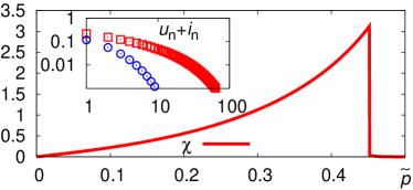
Having obtained the solutions of the recursion relations for a single rooted Cayley tree, we have access to other physical quantities of interest such as the average cluster size or the cluster size distribution in the same recursive manner. For example, the expected size of a cluster containing the root site but not any leaves is given by

$$\chi_{{k}}=\frac{f_{k}F_{k}}{Z_{k}}=\frac{f^{\text{i}}_{k}F^{\text{i}}_{k}+f^{\text{u}}_{k}F^{\text{u}}_{k}}{Z_{k}},$$ (12)

where $f_{k}$ is the average cluster size in non-percolating configurations, $F_{{k}}$ is the weight of corresponding configurations. As before, labels ‘i’ and ‘u’ indicate infected or uninfected clusters. The $k\to\infty$ limit of this quantity plays the role of susceptibility in conventional percolation problems. With minimal effort, it also can be found for the uniform Bethe lattice; the result is shown in Figure S1. Since in our case the transition is first order, this quantity does not diverge at the transition $\tilde{p}=\tilde{p}_{c}$.

The cluster size distribution for a rooted tree can be obtained from the total weight of configurations where the site at level $k$ belongs to a finite cluster

$$F_{k}=F^{\text{i}}_{k}+F^{\text{u}}_{k}=\sum_{n}F^{\text{i}}_{k}(n)+\sum_{n}F^{\text{u}}_{k}(n).$$ (13)

Here $F^{\text{u,i}}_{k}(n)$ are the weights of configurations where the root site belongs to a cluster of size $n$. The corresponding probabilities for a site to belong to an uninfected/infected $n$-site cluster are $(u,i)_{n}=\displaystyle\lim_{k\to\infty}F^{\text{u,i}}_{k}(n)/{Z_{k}}$ and may be also found from recursion relations

$$u_{n}=\tilde{p}\eta\left(\sum^{n-2}_{k\geq 1}u_{k}u_{n-k-1}+2u_{n-1}P_{\text{e}}\right),$$ (14a)

$$i_{n}=\tilde{p}\eta\left(\sum^{n-2}_{k=1}u_{k}u_{n-k-1}+2\sum^{n-2}_{k=1}i_{k}u_{n-k-1}\right.\\ +2P_{\text{e}}i_{n-1}+2P_{\text{e}}u_{n-1}\Bigg{)}.$$ (14b)

Here the probabilities for a site to form an isolated cluster or to remain unoccupied are, respectively,

$$u_{1}=i_{1}=\tilde{p}\eta P^{2}_{\text{e}},\qquad u_{0}=i_{0}=P_{\text{e}}$$ (15)

and $\eta=\lim_{k\to\infty}Z_{k}^{2}/Z_{k+1}$.

The generating functions for both sequences are

$$\mathcal{G}^{\text{u}}(x)=\sum_{n\geq 0}u_{n}x^{n}=\frac{1-\sqrt{1-4x\tilde{p}\eta P_{\text{e}}}}{2x\tilde{p}\eta}$$ (16)

and

$$\mathcal{G}^{\text{i}}(x)=\sum_{n\geq 0}i_{n}x^{n}=\frac{P_{\text{e}}+x\tilde{p}\eta\left[{\mathcal{G}^{\text{u}}}(x)\right]^{2}}{1-2x\tilde{p}\eta{\mathcal{G}^{\text{u}}}(x)},$$ (17)

and its series expansion yields $u_{n}$ and $i_{n}$.

The cluster size distribution (inset of Figure S1) has an exponential cutoff for large clusters both below and above the percolation transition. After the appearance of the giant component the cutoff discontinuously shifts to smaller cluster sizes. A similar cluster size distribution can in principle be obtained for a uniform Bethe lattice yet in practice the recursion relations become extremely unwieldy.

S5. Details of numerical simulations

Figure S2: a) Fourth-order Binder cumulant of density. b) Histograms of density at point where peaks are equally weighed; lines indicate fit to a pair of Gaussian functions.

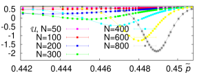
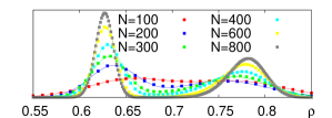
We use a Metropolis Monte-Carlo algorithm developed in Maksymenko2012 on graphs with up to ${N}=820$ sites. The algorithm works in the grand-canonical picture where a chemical potential $\mu$ controls the density of particles $\rho$ and allows it to fluctuate. The statistical weight is $W=\exp{(\mu n)}\prod(n(\mathcal{C}_{i})+1)$. The chemical potential $\mu$ is directly related to the a priori probability $\tilde{p}$ via $\mu=\ln\left[{\tilde{p}/(1-2\tilde{p}})\right]$. At every step we randomly choose a site (or group of sites) and if it is empty (occupied), propose to occupy (empty) it. The new configuration is accepted with a Metropolis probability. We use up to $2\times 10^{6}$ steps for equilibration which are then followed by $2\times 10^{6}$ steps for every measurement round. The plots presented in the report are based on averaging over up to $30$ measurements with a new realization of random graph for every measurement. The expander nature of the graph and the long range of underlying interactions lead to strong hysteresis. To reduce hysteresis, we have employed an exchange Monte-Carlo procedure by simulating the system at different values of $\tilde{p}$ and allowing exchanges of configurations between them. To control hysteresis effects, we have performed simulations starting from empty or occupied lattices as initial conditions. We present results for system sizes which show no hysteresis. In Figure S2 we present a fourth-order Binder cumulant ${\mathcal{U}}$ defined as.

$${\mathcal{U}}=1-\frac{\langle\rho^{4}\rangle}{3\langle\rho^{2}\rangle^{2}}$$ (18)

Minima of this quantity indicates the location of a phase transition, their extrapolation to the thermodynamic limit is plotted in the main text.