Magnetic flux concentrations from dynamo-generated fields

Abstract

Context. The mean-field theory of magnetized stellar convection gives rise to two distinct instabilities: the large-scale dynamo instability, operating in the bulk of the convection zone and a negative effective magnetic pressure instability (NEMPI) operating in the strongly stratified surface layers. The latter might be important in connection with magnetic spot formation. However, the growth rate of NEMPI is suppressed with increasing rotation rates. On the other hand, recent direct numerical simulations (DNS) have shown a subsequent increase in the growth rate.

Aims. We examine quantitatively whether this increase in the growth rate of NEMPI can be explained by an $\alpha^{2}$ mean-field dynamo, and whether both NEMPI and the dynamo instability can operate at the same time.

Methods. We use both DNS and mean-field simulations (MFS) to solve the underlying equations numerically either with or without an imposed horizontal field. We use the test-field method to compute relevant dynamo coefficients.

Results. DNS show that magnetic flux concentrations are still possible up to rotation rates above which the large-scale dynamo effect produces mean magnetic fields. The resulting DNS growth rates are quantitatively reproduced with MFS. As expected for weak or vanishing rotation, the growth rate of NEMPI increases with increasing gravity, but there is a correction term for strong gravity and large turbulent magnetic diffusivity.

Conclusions. Magnetic flux concentrations are still possible for rotation rates above which dynamo action takes over. For the solar rotation rate, the corresponding turbulent turnover time is about 5 hours, with dynamo action commencing in the layers beneath.

1 Introduction

The appearance of surface magnetic fields in the Sun presents some peculiar characteristics, such as being strongly concentrated into discrete spots. The origin and depth of such magnetic flux concentrations has long been the subject of considerable speculation. A leading theory by Parker (1955) interprets the emergence of such spots as the result of magnetically buoyant flux tubes at a depth of some 20 Mm. This magnetic field must be the result of a dynamo, but magnetic buoyancy also leads to the buoyant rise and subsequent loss of those magnetic structures. It was therefore thought that the dynamo should operate mainly at or even below the bottom of the convection zone where magnetic buoyancy could be stabilized by a subadiabatic temperature gradient (Parker, 1975). This led eventually to the idea that sunspots might be a direct consequence of dynamo-generated flux tubes that rise all the way from the bottom of the convection zone to the surface (e.g., Caligari et al., 1995). However, Schüssler (1980, 1983) emphasized early on that such fields would easily lose their systematic east–west orientation while ascending through the turbulent convection zone. D’Silva & Choudhuri (1993) estimated that a magnetic field strength of about $100\,{\rm kG}$ would be needed to preserve the overall east–west orientation (Hale et al., 1919) and also to produce the observed tilt angle of active regions known as Joy’s law.

A great deal of effort has gone into determining the conditions under which magnetic flux ropes may or may not be able to rise buoyantly across the convection zone. Emonet et al. (1998) determined for the first time the basic minimum twist thresholds for the survival of twisted magnetic flux ropes during the rise. Subsequent studies were based on different types of numerical simulations, which tested the underlying hypotheses and looked for other effects, such as the robustness against background convective motions (Jouve et al., 2013) and magnetic flux erosion by reconnection with the background dynamo field (Pinto et al., 2013). These studies, as well as many others (see, e.g., Fan, 2008, 2009, and references therein) specifically looked at which flux-rope configurations are able to reproduce the observed emergent polarity tilt angles (Joy’s law).

The observed variation in the number of sunspots in time and latitude is expected to be linked to some kind of large-scale dynamo, as was modeled by Leighton et al. (1969) and Steenbeck & Krause (1969) long ago. This led Schüssler (1980) to propose a so-called flux-tube dynamo approach that would couple the buoyant rise of thin flux tubes to their regeneration. However, even today the connection between dynamos and flux tubes is done by hand (see, e.g., Choudhuri et al., 2007; Miesch & Dikpati, 2014), which means that an ad hoc procedure is invoked to link flux tube emergence to a mean-field dynamo. Of course, such tubes, or at least bipolar regions, should ultimately emerge from a sufficiently well-resolved and realistic simulation of solar convection. While global convective dynamo simulations of Nelson et al. (2011, 2013, 2014) show magnetically buoyant magnetic flux tubes of $\approx 40\,{\rm kG}$ field strength, they do not yet address bipolar region formation. Indeed, solar surface simulations of Cheung et al. (2010) and Rempel & Cheung (2014) demonstrate that bipolar spots do form once a magnetic flux tube of $10\,{\rm kG}$ field strength is injected at the bottom of their local domain ($7.5\,{\rm Mm}$ below the surface). On the other hand, the deep solar simulations of Stein & Nordlund (2012) develop a bipolar active region with just $1\,{\rm kG}$ magnetic field injected at the bottom of their domain. While these simulations taken together outline what might occur in the Sun, they do not necessarily support the description of spots as a direct result of thin flux tubes piercing the surface (e.g. Caligari et al., 1995).

A completely different suggestion is that sunspots develop locally at the solar surface, and that their east–west orientation would reflect the local orientation of the mean magnetic field close to the surface. The tilt angle would then be determined by latitudinal shear producing the observed orientation of the meridional component of the magnetic field (Brandenburg, 2005a). One of the possible mechanisms of local spot formation is the negative effective magnetic pressure instability (NEMPI; see Kleeorin et al., 1989, 1990; Kleeorin & Rogachevskii, 1994; Kleeorin et al., 1996; Rogachevskii & Kleeorin, 2007). Another potential mechanism of flux concentration is related to a thermo-magnetic instability in turbulence with radiative boundaries caused by the suppression of turbulent heat flux through the large-scale magnetic field (Kitchatinov & Mazur, 2000). The second instability has so far only been found in mean-field simulations (MFS), but not in direct numerical simulations (DNS) nor in large-eddy simulations (LES). By contrast, NEMPI has recently been found in DNS (Brandenburg et al., 2011) and LES (Brandenburg et al., 2014) of strongly stratified fully developed turbulence.

As demonstrated in earlier work (Brandenburg et al., 2013, 2014), NEMPI can lead to the formation of equipartition-strength magnetic spots, which are reminiscent of sunspots. Even bipolar spots can form in the presence of a horizontal magnetic field near the surface (see Warnecke et al., 2013). For this idea to be viable, NEMPI and the dynamo instability would need to operate in reasonable proximity to each other, so that the dynamo can supply the magnetic field that would be concentrated into spots, as was recently demonstrated by Mitra et al. (2014). In studying this process in detail, we have a chance of detecting new joint effects resulting from the two instabilities, which is one of the goals of the present paper. However, these two instabilities may also compete against each other, as was already noted by Losada et al. (2013). The large-scale dynamo effect relies on the combined presence of rotation and stratification, while NEMPI requires stratification and large enough scale separation. On the other hand, even a moderate amount of rotation suppresses NEMPI. In fact, Losada et al. (2012) found significant suppression of NEMPI when the Coriolis number $\mbox{\rm Co}=2\Omega\tau$ is larger than about 0.03. Here, $\Omega$ is the angular velocity and $\tau$ the turnover time of the turbulence, which is related to the rms velocity $u_{\rm rms}$ and the wavenumber $k_{\rm f}$ of the energy-carrying eddies via $\tau=(u_{\rm rms}k_{\rm f})^{-1}$. For the solar convection zone, the Coriolis number,

$$\mbox{\rm Co}=2\Omega/u_{\rm rms}k_{\rm f},$$ (1)

varies from $2\times 10^{-3}$ (at the surface using $\tau=5\min$) to $5$ (at the bottom of the convection zone using $\tau=10\,{\rm days}$). The value $\mbox{\rm Co}=0.03$ corresponds to a turnover time as short as two hours, which is the case at a depth of $\approx 10\,{\rm Mm}$.

The strength of stratification, on the other hand, is quantified by the nondimensional parameter

$$\mbox{\rm Gr}=g/c_{\rm s}^{2}k_{\rm f}\equiv(k_{\rm f}H_{\rho})^{-1},$$ (2)

where $H_{\rho}=c_{\rm s}^{2}/g$ is the density scale height, $c_{\rm s}$ is the sound speed, and $g$ is the gravitational acceleration. In the cases considered by Losada et al. (2012, 2013), the stratification parameter was $\mbox{\rm Gr}=0.03$, which is rather small compared with the estimated solar value of $\mbox{\rm Gr}=0.16$ (see the conclusions of Losada et al., 2013). One can expect that larger values of Gr would result in correspondingly larger values of the maximum permissible value of Co, for which NEMPI is still excited, but this has not yet been investigated in detail.

The goal of the present paper is to study rotating stratified hydromagnetic turbulence in a parameter regime that we expect to be at the verge between NEMPI and dynamo instabilities. We do this by performing DNS and MFS. In MFS, the study of combined NEMPI and dynamo instability requires suitable parameterizations of the negative effective magnetic pressure and $\alpha$ effects using suitable turbulent transport coefficients.

2 DNS study

We begin by reproducing some of the DNS results of Losada et al. (2013), who found the suppression of the growth rate of NEMPI with increasing values of Co and a subsequent enhancement at larger values, which they interpreted as being the result of dynamo action in the presence of an externally applied magnetic field. We also use DNS to determine independently the expected efficiency of the dynamo by estimating the $\alpha$ effect from kinetic helicity measurements and by computing both $\alpha$ effect and turbulent diffusivity directly using the test-field method (TFM).

2.1 Basic equations

In DNS of an isothermally stratified layer (Losada et al., 2013), we solve the equations for the velocity $U$, the magnetic vector potential $A$, and the density $\rho$ in the presence of rotation $\Omega$,

$${{\rm D}{}\mbox{\boldmath$U$}{}\over{\rm D}{}t} = {1\over\rho}\mbox{\boldmath$J$}{}\times\bm{B}-2\bm{\Omega}\times\mbox{\boldmath$U$}{}-\nu\mbox{\boldmath$Q$}{}+\mbox{\boldmath$F$}{}+\mbox{\boldmath$f$}{},$$ (3)

$${\partial\mbox{\boldmath$A$}{}\over\partial t} = \mbox{\boldmath$U$}{}\times\bm{B}-\eta\mbox{\boldmath$J$}{},$$ (4)

$${\partial\rho\over\partial t} = -\mbox{\boldmath$\nabla$}{}\cdot\rho\mbox{\boldmath$U$}{},$$ (5)

where ${\rm D}{}/{\rm D}{}t=\partial/\partial t+\mbox{\boldmath$U$}{}\cdot\mbox{\boldmath$\nabla$}{}$ is the advective derivative, $\bm{\Omega}=\Omega\hat{\mbox{\boldmath$z$}}{}$ is the angular velocity,

$$\mbox{\boldmath$F$}{}=\mbox{\boldmath$g$}{}-c_{\rm s}^{2}\mbox{\boldmath$\nabla$}{}\ln\rho$$ (6)

determines the hydrostatic force balance, $\nu$ is the kinematic viscosity, $\eta$ is the magnetic diffusivity due to Spitzer conductivity of the plasma,

$$-\mbox{\boldmath$Q$}{} = \nabla^{2}\mbox{\boldmath$U$}{}+\mbox{\boldmath$\nabla$}{}\mbox{\boldmath$\nabla$}{}\cdot\mbox{\boldmath$U$}{}/3+2\mbox{\boldmath${\sf S}$}{}\mbox{\boldmath$\nabla$}{}\ln\rho,$$ (7)

$$-\mbox{\boldmath$J$}{} = \nabla^{2}\mbox{\boldmath$A$}{}-\mbox{\boldmath$\nabla$}{}\mbox{\boldmath$\nabla$}{}\cdot\mbox{\boldmath$A$}{},$$ (8)

are the modified vorticity and the current density, respectively, where the vacuum permeability $\mu_{0}$ has been set to unity,

$$\bm{B}=\bm{B}_{0}+\mbox{\boldmath$\nabla$}{}\times\mbox{\boldmath$A$}{}$$ (9)

is the total magnetic field, $\bm{B}_{0}=(0,B_{0},0)$ is the imposed uniform field, and

$${\sf S}_{ij}={\textstyle{1\over 2}}(\partial_{j}U_{i}+\partial_{i}U_{j})-{\textstyle{1\over 3}}\delta_{ij}\mbox{\boldmath$\nabla$}{}\cdot\mbox{\boldmath$U$}{}$$ (10)

is the traceless rate-of-strain tensor. The forcing function $f$ consists of random, white-in-time, plane, nonpolarized waves with a certain average wavenumber $k_{\rm f}$. The turbulent rms velocity is approximately independent of $z$ with $u_{\rm rms}=\langle\mbox{\boldmath$u$}{}^{2}\rangle^{1/2}\approx 0.1\,c_{\rm s}$. The gravitational acceleration $\mbox{\boldmath$g$}{}=(0,0,-g)$ is chosen such that $k_{1}H_{\rho}=1$, so the density contrast between bottom and top is $\exp(2\pi)\approx 535$ in a domain $-\pi\leq k_{1}z\leq\pi$. Here, $H_{\rho}=c_{\rm s}^{2}/g$ is the density scale height and $k_{1}=2\pi/L$ is the smallest wavenumber that fits into the cubic domain of size $L^{3}$. We adopt Cartesian coordinates $(x,y,z)$, with periodic boundary conditions in the $x$ and $y$ directions and stress-free, perfectly conducting boundaries at top and bottom ($z=\pm L_{z}/2$). In most of the calculations, we use a scale separation ratio $k_{\rm f}/k_{1}$ of 30, so $\mbox{\rm Gr}=0.03$ is still the same as in earlier calculations. We use a fluid Reynolds number $\mbox{\rm Re}\equiv u_{\rm rms}/\nu k_{\rm f}$ of 36, and a magnetic Prandtl number $\mbox{\rm Pr}_{M}=\nu/\eta$ of 0.5. The magnetic Reynolds number is therefore $\mbox{\rm Re}_{M}=\mbox{\rm Pr}_{M}\mbox{\rm Re}=18$. These values are a compromise between having both $k_{\rm f}$ and Re large enough for NEMPI to develop at an affordable numerical resolution. The value of $B_{0}$ is specified in units of $B_{\rm eq0}=\sqrt{\rho_{0}}\,u_{\rm rms}$, where $\rho_{0}=\langle\rho\rangle$ is the volume-averaged density, which is constant in time. The local equipartition field strength is $B_{\rm eq}(z)=\sqrt{\rho}\,u_{\rm rms}$. In our units, $k_{1}=c_{\rm s}=\mu_{0}=\rho_{0}=1$. However, time is specified as the turbulent-diffusive time $t\,\eta_{\rm t0}k_{1}^{2}$, where $\eta_{\rm t0}=u_{\rm rms}/3k_{\rm f}$ is the estimated turbulent diffusivity. We also use DNS to compute these values more accurately with the TFM. The simulations are performed with the Pencil Code (http://pencil-code.googlecode.com), which uses sixth-order explicit finite differences in space and a third-order accurate time-stepping method. We use a numerical resolution of $256^{3}$ mesh points, which was found to be sufficient for the parameter regime specified above.

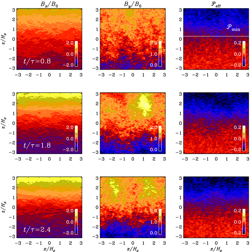
Figure 1: Visualization of $\overline{B}_{x}/B_{0}$ and $\overline{B}_{y}/B_{0}$ together with effective magnetic pressure for different times. Here $\Omega=0.15$, $\mbox{\rm Co}=0.09$, $\mbox{\rm Gr}=0.033$, and $k_{\rm f}/k_{1}=30$.

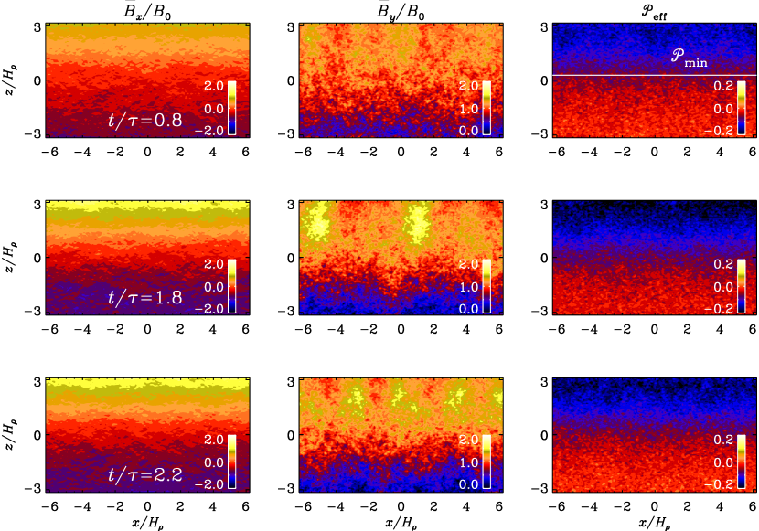
Figure 2: Like Fig. 1, but for a wider domain.

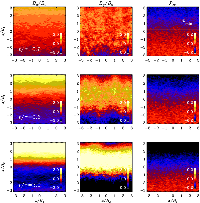
Figure 3: Like Fig. 1, but for $\Omega=0.35$, so $\mbox{\rm Co}=0.22$.

2.2 At the verge between NEMPI and dynamo

The work of Losada et al. (2013) suggested that for $\mbox{\rm Gr}=0.03$ and $\mbox{\rm Co}\geq 0.03$, NEMPI becomes strongly suppressed, and that for still larger values, the growth rate increases again. This was tentatively associated with dynamo action, but it was not investigated in further detail. We now consider such a case with $\mbox{\rm Co}=0.09$. This is a value that resulted in a rather low growth rate for NEMPI, while the estimated growth rate would be still subcritical for dynamo action. Following the work of Losada et al. (2013), we impose here a horizontal magnetic field in the $y$ direction with a strength of $0.05B_{\rm eq0}$, which was previously found to be in the optimal range for NEMPI to develop (Kemel et al., 2012a).

To bring out the structures more clearly, it was found to be advantageous to present mean magnetic fields by averaging over the $y$ direction and over a certain time interval $\Delta t$. We denote such averages by an overbar, e.g., $\overline{B}_{y}$. Once a dynamo develops, we expect a Beltrami-type magnetic field with $\overline{B}_{x}$ phase shifted relative to $\overline{B}_{y}$ by $\pi/2$ (Brandenburg, 2001). These are force-free fields with $\mbox{\boldmath$\nabla$}{}\times\overline{\mbox{\boldmath$B$}}{}=k\overline{\mbox{\boldmath$B$}}{}$ such as $\overline{\mbox{\boldmath$B$}}{}\propto(\sin kz,\cos kz,0)$, for example.

Figure 1 shows visualizations of $\overline{B}_{x}$ and $\overline{B}_{y}$ together with the effective magnetic pressure, ${\cal P}_{\rm eff}$ (defined below), at different times for a value of Co that is around the point where we expect onset of dynamo action. As in earlier work without rotation (Kemel et al., 2013), $\overline{B}_{y}$ varies between 0 to $2B_{0}$. Furthermore, $\overline{B}_{x}$ varies in the range $\pm 2B_{0}$. In Fig. 2, the $x$ extent of the domain is twice as big: $-2\pi<k_{1}x<2\pi$. In Fig. 3 we show the result for $\mbox{\rm Co}=0.22$, where a Beltrami-type field with a $\pi/2$ phase shift between $\overline{B}_{x}$ and $\overline{B}_{y}$ is well developed. For smaller values of Co, there are structures (e.g., for $t/\tau=1.8$ at $x/H_{\rho}\approx 1.5$ and for $t/\tau=2.4$ at $x/H_{\rho}\approx 1.5$ and $-2$) that are reminiscent of those associated with NEMPI. This can be seen by comparing our Fig. 1 with Fig. 4 of Kemel et al. (2013) or Fig. 3 of Losada et al. (2013). When the domain is twice as wide, the number of structures simply doubles. A similar phenomenon was also seen in the simulations of Kemel et al. (2012b). For larger values of Co, NEMPI is suppressed and the $\alpha^{2}$ dynamo, which generates mean magnetic field of a Beltrami-type structure, becomes more strongly excited.

The effective magnetic pressure shown in Figs. 1–3 is estimated by computing the $xx$ component of the total stress from the fluctuating velocity and magnetic fields as

$$\Delta\overline{\Pi}_{xx}^{\rm f}=\overline{\rho}\,(\overline{u_{x}^{2}}-\overline{u_{0x}^{2}})+{\textstyle{1\over 2}}(\overline{\bm{b}^{2}}-\overline{\bm{b}_{0}^{2}})-(\overline{b_{x}^{2}}-\overline{b_{0x}^{2}}),$$ (11)

where the subscript $0$ refers to the case with $B_{0}=0$. We then calculate (Brandenburg et al., 2012a)

$$q_{\rm p}=-2\Delta\overline{\Pi}_{xx}^{\rm f}/\overline{\mbox{\boldmath$B$}}{}^{2}.$$ (12)

Here, $q_{\rm p}(\beta)$ is a function of $\beta=\overline{B}/B_{\rm eq}(z)$. We then calculate ${\cal P}_{\rm eff}={\textstyle{1\over 2}}(1-q_{\rm p})\beta^{2}$, which is the effective magnetic pressure divided by $B_{\rm eq}^{2}$. We note that ${\cal P}_{\rm eff}$ shows a systematic $z$ dependence and is negative in the upper part. Variations in the $x$ direction are comparatively weak and therefore do not show a clear correspondence with the horizontal variations of $\overline{B}_{y}$.

As in earlier work (Brandenburg et al., 2011), we characterize the strength of resulting structures by an amplitude $B_{k}$ of a suitably low wavenumber Fourier mode ($k/k_{1}=1$ or 2), which is based on the magnetic field in the upper part of the domain, $2\leq z/H_{\rho}\leq\pi$. In Fig. 4 we compare the evolution of $B_{k}/B_{\rm eq0}$ for runs with different values of Co. For comparison, we also reproduce the first few runs of Losada et al. (2013) for $\mbox{\rm Co}=0.006$–$0.13$, where we used $k/k_{1}=1$ in all cases. It turns out that for the new cases with $\mbox{\rm Co}=0.09$ and $0.22$, the growth of $B_{k}/B_{\rm eq0}$ is not as strong as for the cases with smaller Co. Furthermore, as is also evident from Figs. 1 and 2, the structures are now characterized by $k/k_{1}=2$, while for $\mbox{\rm Co}=0.22$ they are still characterized by $k/k_{1}=1$. The growth for all three cases ($\mbox{\rm Co}=0.09$, both for normal and wider domains, as well as $\mbox{\rm Co}=0.22$) is similar. However, given that the typical NEMPI structures are not clearly seen for $\mbox{\rm Co}=0.22$, it is possible that the growth of structures is simply overwhelmed by the much stronger growth due to the dynamo, which is not reflected in the growth of $B_{k}/B_{\rm eq0}$, whose growth is still mainly indicative of NEMPI. In this sense, there is some evidence of the occurrence of NEMPI in both cases.

2.3 Kinetic helicity

To estimate the $\alpha$ effect and study its relation to kinetic helicity we begin by considering a fixed value of Gr equal to that used by Losada et al. (2013) and vary Co. For small values of Co, their data agreed with the MFS of Losada et al. (2012). For faster rotation, one eventually crosses the dynamo threshold. This is also the point at which the growth rate begins to increase again, although it now belongs to a different instability than for small values of Co. The underlying mechanism is the $\alpha^{2}$-dynamo, which is characterized by the dynamo number

$$C_{\alpha}=\alpha/\eta_{\rm T}k_{1},$$ (13)

where $\alpha$ is the typical value of the $\alpha$ effect (here assumed spatially constant), $\eta_{\rm T}=\eta_{\rm t}+\eta$ is the sum of turbulent and microphysical magnetic diffusivities, and $k_{1}$ is the lowest wavenumber of the magnetic field that can be fitted into the domain. For isotropic turbulence, $\alpha$ and $\eta_{\rm t}$ are respectively proportional to the negative kinetic helicity and the mean squared velocity (Moffatt, 1978; Krause & Rädler, 1980; Rädler et al., 2003; Kleeorin & Rogachevskii, 2003)

$$\alpha\approx\alpha_{0}\equiv-{\textstyle{1\over 3}}\tau\overline{\mbox{\boldmath$\omega$}{}\cdot\mbox{\boldmath$u$}{}},\quad\eta_{\rm t}\approx\eta_{\rm t0}\equiv{\textstyle{1\over 3}}\tau\overline{\mbox{\boldmath$u$}{}^{2}},$$ (14)

where $\tau=(u_{\rm rms}k_{\rm f})^{-1}$, so that (Blackman & Brandenburg, 2002; Candelaresi & Brandenburg, 2013)

$$C_{\alpha}=-\epsilon_{\it k}\epsilon_{\rm f}k_{\rm f}/k_{1}.$$ (15)

Here, $\epsilon_{\it k}$ is a free parameter characterizing possible dependencies on the forcing wavenumber, and $\epsilon_{\rm f}$ is a measure for the relative kinetic helicity. Simulations of Brandenburg et al. (2012b) and Losada et al. (2013) showed that

$$\epsilon_{\rm f}\equiv\overline{\mbox{\boldmath$\omega$}{}\cdot\mbox{\boldmath$u$}{}}/k_{\rm f}u_{\rm rms}^{2}\approx\epsilon_{\rm f0}\,\mbox{\rm Gr}\,\mbox{\rm Co}\quad(\mbox{\rm Gr}\,\mbox{\rm Co}\mathrel{\mathchoice{\vbox{\offinterlineskip\halign{\hfil$\displaystyle#$\hfil\cr<\cr\sim\cr}}}{\vbox{\offinterlineskip\halign{\hfil$\textstyle#$\hfil\cr<\cr\sim\cr}}}{\vbox{\offinterlineskip\halign{\hfil$\scriptstyle#$\hfil\cr<\cr\sim\cr}}}{\vbox{\offinterlineskip\halign{\hfil$\scriptscriptstyle#$\hfil\cr<\cr\sim\cr}}}}0.1),$$ (16)

where $\epsilon_{\rm f0}$ is yet another non-dimensional parameter on the order of unity that may depend weakly on the scale separation ratio, $k_{\rm f}/k_{1}$, and is slightly different with and without imposed field. In the absence of an imposed field, Brandenburg et al. (2012b) found $\epsilon_{\rm f0}\approx 2$ using $k_{\rm f}/k_{1}=5$. However, both an imposed field and a larger value of $k_{\rm f}/k_{1}$ lead to a slightly increased value of $\epsilon_{\rm f0}$. Our results are summarized in Fig. 5 for cases with and without imposed magnetic fields. Error bars are estimated as the largest departure of any one third of the full time series. The relevant points of Losada et al. (2013) give $\epsilon_{\rm f0}\approx 2.8$. For $\mbox{\rm Gr}\,\mbox{\rm Co}\mathrel{\mathchoice{\vbox{\offinterlineskip\halign{\hfil$\displaystyle#$\hfil\cr>\cr\sim\cr}}}{\vbox{\offinterlineskip\halign{\hfil$\textstyle#$\hfil\cr>\cr\sim\cr}}}{\vbox{\offinterlineskip\halign{\hfil$\scriptstyle#$\hfil\cr>\cr\sim\cr}}}{\vbox{\offinterlineskip\halign{\hfil$\scriptscriptstyle#$\hfil\cr>\cr\sim\cr}}}}0.5$, the results of Brandenburg et al. (2012b) show a maximum with a subsequent decline of $\epsilon_{\rm f}$ with increasing values of Co. However, although it is possible that the position of this maximum may be different for other values of Gr, it is unlikely to be relevant to our present study where we focus on smaller values of $C_{\alpha}$ near dynamo onset. Thus, in conclusion, Eq. (16) seems to be a useful approximation that has now been verified over a range of different values of $k_{\rm f}/k_{1}$.

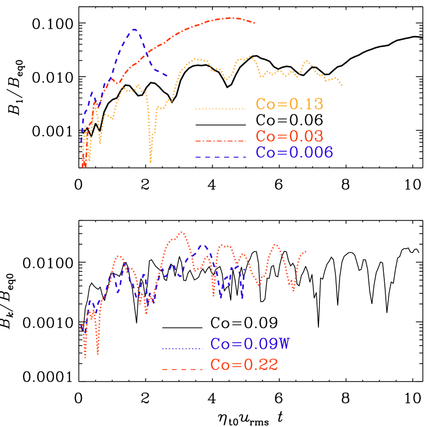
Figure 4: Comparison of the evolution of $B_{k}/B_{\rm eq0}$ for runs with different values of Co. In the first panel $k/k_{1}=1$, while in the second panel $k/k_{1}=2$ for the two runs with $\mbox{\rm Co}=0.09$ (label W refers to the wider box in the $x$ direction), and $k/k_{1}=1$ for the run with $\mbox{\rm Co}=0.22$.

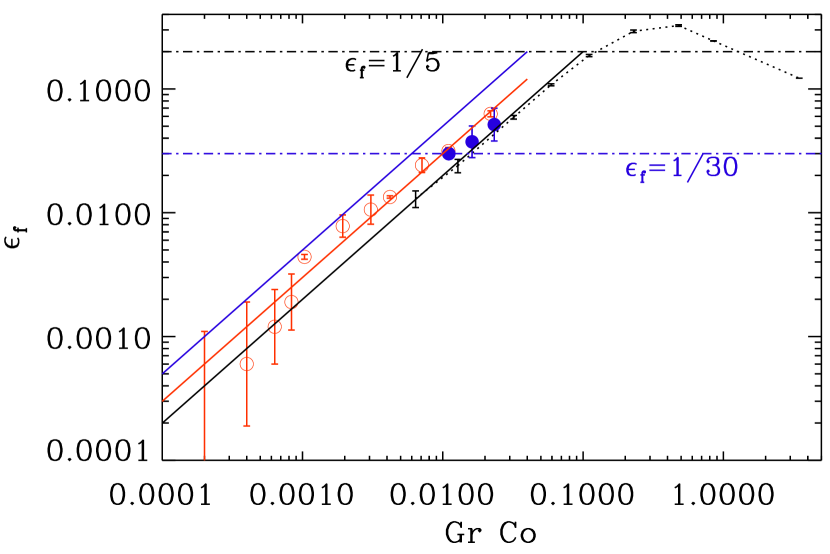
Figure 5: Dependence of $\epsilon_{\rm f}$ on Gr Co obtained in DNS with imposed field (open symbols, red) and without (closed symbols, blue), for $k_{\rm f}/k_{1}=30$. The black symbols connected by a dotted line correspond to the values of Brandenburg et al. (2012b) for $k_{\rm f}/k_{1}=5$. The horizontal lines correspond to the dynamo threshold for the two values of $k_{\rm f}/k_{1}$.

2.4 Test-field results

Our estimate for $C_{\alpha}$ is based on the reference values $\alpha_{0}$ and $\eta_{\rm t0}$ that are defined in Eq. (14) and represent approximations obtained from earlier simulations of helically forced turbulence (Sur et al., 2008). In the present study, helicity is self-consistently generated from the interaction between rotation and stratification. As an independent way of computing $\alpha$ and $\eta_{\rm t}$, we now use the test-field method (TFM). It consists of solving auxiliary equations describing the evolution of magnetic fluctuations, $\bm{b}^{pq}$, resulting from a set of several prescribed mean or test fields, $\overline{\mbox{\boldmath$B$}}{}^{pq}$. We solve for the corresponding vector potential $\mbox{\boldmath$a$}{}^{pq}$ with $\bm{b}^{pq}=\mbox{\boldmath$\nabla$}{}\times\mbox{\boldmath$a$}{}^{pq}$,

$${\partial\mbox{\boldmath$a$}{}^{pq}\over\partial t}=\mbox{\boldmath$u$}{}\times\overline{\mbox{\boldmath$B$}}{}^{pq}+\overline{\mbox{\boldmath$U$}}{}\times\bm{b}^{pq}+(\mbox{\boldmath$u$}{}\times\bm{b}^{pq})^{\prime}+\eta\nabla^{2}\mbox{\boldmath$a$}{}^{pq},$$ (17)

where $(\mbox{\boldmath$u$}{}\times\bm{b}^{pq})^{\prime}=\mbox{\boldmath$u$}{}\times\bm{b}^{pq}-\overline{\mbox{\boldmath$u$}{}\times\bm{b}^{pq}}$ is the fluctuating part of the electromotive force and

$$\overline{\mbox{\boldmath$B$}}{}^{i{\rm c}}=\hat{\mbox{\boldmath$x$}}{}_{i}\cos kz,\quad\overline{\mbox{\boldmath$B$}}{}^{i{\rm s}}=\hat{\mbox{\boldmath$x$}}{}_{i}\sin kz,\quad i=1,2,$$ (18)

are the four test fields, which can show a cosine or sine variation with $z$, while $\hat{\mbox{\boldmath$x$}}{}_{1}=(1,0,0)$ and $\hat{\mbox{\boldmath$x$}}{}_{2}=(0,1,0)$ are unit vectors in the two horizontal coordinate directions. The resulting $\bm{b}^{pq}$ are used to compute the electromotive force, $\overline{\mbox{\boldmath${\cal E}$}}{}^{pq}=\overline{\mbox{\boldmath$u$}{}\times\bm{b}^{pq}}$, which is then expressed in terms of $\overline{\mbox{\boldmath$B$}}{}^{pq}$ and $\overline{\mbox{\boldmath$J$}}{}^{pq}=\mbox{\boldmath$\nabla$}{}\times\overline{\mbox{\boldmath$B$}}{}^{pq}$ as

$$\overline{\cal E}{}^{pq}_{i}=\alpha_{ij}\overline{B}^{pq}_{j}-\eta_{ij}\overline{J}^{pq}_{j}.$$ (19)

By doing this for all four test field vectors, the $x$ and $y$ components of each of them gives eight equations for the eight unknowns, $\alpha_{11}$, $\alpha_{12}$, …, $\eta_{22}$ (for details see Brandenburg, 2005b).

With the TFM, we obtain the kernels $\alpha_{ij}$ and $\eta_{ij}$, from which we compute

$$\alpha={\textstyle{1\over 2}}(\alpha_{11}+\alpha_{22}),\quad\eta_{\rm t}={\textstyle{1\over 2}}(\eta_{11}+\eta_{22}),$$ (20)

$$\gamma={\textstyle{1\over 2}}(\alpha_{21}-\alpha_{12}),\quad\delta={\textstyle{1\over 2}}(\eta_{21}-\eta_{12}).$$ (21)

We normalize $\alpha$ and $\eta_{\rm t}$ by their respective values obtained for large magnetic Reynolds numbers defined in Eq. (14), and denote them by a tilde, i.e., $\tilde{\alpha}=\alpha/\alpha_{0}$ and $\tilde{\eta}_{\rm t}=\eta_{\rm t}/\eta_{\rm t0}$. We use the latter normalization also for $\delta$, i.e., $\tilde{\delta}=\delta/\eta_{\rm t0}$, but expect its value to vanish in the limit of zero angular velocity. No standard turbulent pumping velocity is expected (Krause & Rädler, 1980; Moffatt, 1978), because the rms turbulent velocity is independent of height. However, this is not quite true. To show this, we normalize $\gamma$ by $u_{\rm rms}$ and present $\tilde{\gamma}=\gamma/u_{\rm rms}$. In our normalization, the molecular value is given by

$\eta/\eta_{0}=3/\mbox{\rm Re}_{M}$.

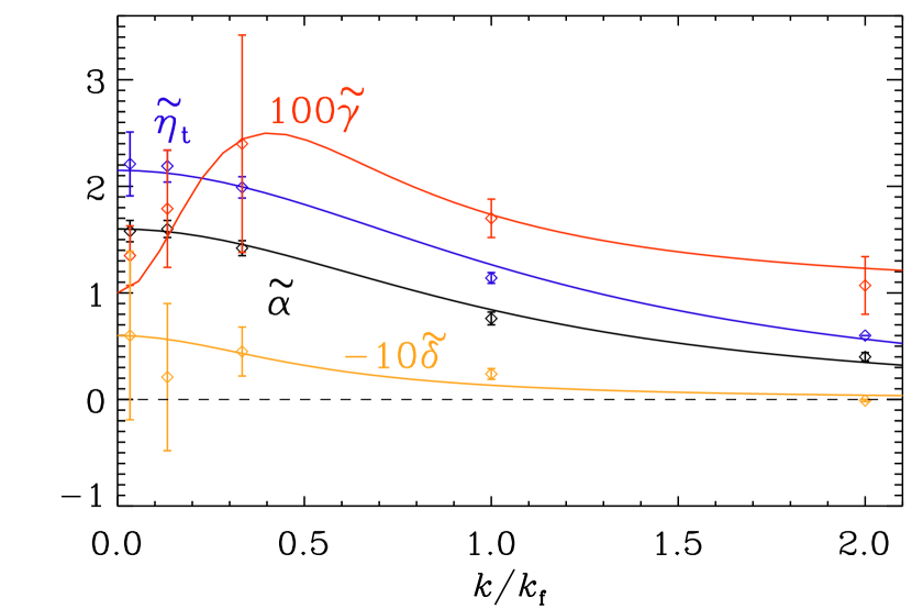
Figure 6: TFM coefficients versus scale separation ratio, $k/k_{\rm f}$, for $\mbox{\rm Co}=0.59$, $\mbox{\rm Re}_{M}=18$, $B_{0y}/B_{\rm eq0}=0.05$, $\tilde{g}=1$, and $\eta k_{1}/c_{\rm s}=2\times 10^{-4}$.

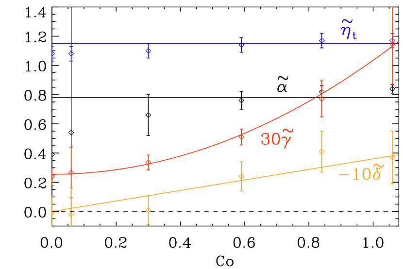
Figure 7: TFM coefficients versus Coriolis number, Co, for $k/k_{1}=1$, $\mbox{\rm Re}_{M}=18$, $B_{0y}/B_{\rm eq0}=0.05$, $\tilde{g}=1$, and $\eta k_{1}/c_{\rm s}=2\times 10^{-4}$.

We consider test fields that are constant in time and vary sinusoidally in the $z$ direction. We choose certain values of $k$ between $k_{1}$ and $60k_{\rm f}$ (=$2k_{1})$ and also vary the value of Co between 0 and about 1.06 while keeping $\mbox{\rm Gr}=0.033$ fixed. In all cases where the scale separation ratio is held fixed, we used $k_{\rm f}/k_{1}\approx 30$, which is larger than what has been used in earlier studies (Brandenburg et al., 2008b), where $k_{\rm f}/k_{1}$ was typically 5.

In Figure 6 we show the dependence of the coefficients on the normalized wavenumber of the test field, $k/k_{\rm f}$. The three coefficients $\tilde{\alpha}$, $\tilde{\eta}_{\rm t}$, and $\tilde{\delta}$ show the same behavior of the form of

$$\tilde{\sigma}=\tilde{\sigma}_{0}/\left(1+\ell_{\sigma}^{2}k^{2}\right)$$ (22)

for $\tilde{\sigma}=\tilde{\alpha}$, $\tilde{\eta}_{\rm t}$, or $\tilde{\delta}$, while for $\tilde{\gamma}$ we use

$$\tilde{\gamma}=\tilde{\gamma}_{0}+\tilde{\gamma}_{2}\ell_{\gamma}^{2}k^{2}/\left(1+\ell_{\gamma}^{2}k^{2}\right),$$ (23)

where $\tilde{\gamma}_{0}=0.01$, $\tilde{\gamma}_{2}=0.06$, and $\ell_{\gamma}=2.5$. These results have been obtained for $\mbox{\rm Co}=0.59$ and $B_{0y}/B_{\rm eq0}=0.05$. Again, error bars are estimated as the largest departure of any one third of the full time series.

Most of the coefficients are only weakly dependent on the value of Co, except $\gamma$ and $\delta$. The former varies approximately as

$$\tilde{\gamma}=\tilde{\gamma}_{0}+\tilde{\gamma}_{\Omega}^{2}\mbox{\rm Co}^{2},$$ (24)

where $\tilde{\gamma}_{0}=0.85$ and $\tilde{\gamma}_{\Omega}^{2}=2.6$. Here and in the following, we keep $k/k_{\rm f}=1/30$. For the same value of $k/k_{\rm f}$, the functional form for $\delta$ shows a linear increase with Co, i.e., $\tilde{\delta}=\tilde{\delta}_{0}\mbox{\rm Co}$ where $\tilde{\delta}_{0}=0.036$. Figure 7 shows that $\tilde{\alpha}$ is nearly independent of the Coriolis number. This result is in agreement with that obtained Kleeorin & Rogachevskii (2003), where a theory of $\alpha$ versus Coriolis number was developed for large fluid and magnetic Reynolds numbers. It turns out that the new values of $\alpha$ and $\eta_{\rm t}$ that have been obtained now with the TFM are somewhat different from previous TFM studies that originally estimated ($\tilde{\alpha}\approx 0.8$ and $\tilde{\eta}_{\rm t}\approx 1.15$). The TFM results now suggest $\epsilon_{\it k}=0.6$ in Eq. (15). The reason for the departure from unity cannot just be the fact that helicity is now self-consistently generated, because this was also the case in the earlier work of Brandenburg et al. (2012b). The only plausible reason is the large value of $k_{\rm f}/k_{1}$ that is now much larger than before ($30$ compared to $5$ in most previous studies), which explains the reason for our choice of the subscript in $\epsilon_{\it k}$.

The origin of weak pumping found in Figs. 6 and 7 is unclear. For a weak mean magnetic field, pumping of the magnetic field can cause not only inhomogeneous distributions of the velocity fluctuations (Krause & Rädler, 1980; Moffatt, 1978) or magnetic fluctuations (Rädler et al., 2003), but also non-uniform distribution of the fluid density in the presence either of small-scale dynamo or turbulent convection (Rogachevskii & Kleeorin, 2006). In our simulations there is no small-scale dynamo effect, because $\mbox{\rm Re}_{M}$ is too low. There is also no turbulent convection possible in our setup. The pumping effect is also not connected with nonlinear effects; see Fig. 2 in Rogachevskii & Kleeorin (2004).

3 MFS study

We now want to see whether the suppression of NEMPI and the subsequent increase in the resulting growth rate can be reproduced in MFS. In addition to a parameterization for the negative effective magnetic pressure in the momentum equation, we add one for the electromotive force. The important terms here are the $\alpha$ effect and the turbulent magnetic diffusivity, whose combined effect is captured by the quantity $C_{\alpha}$, which is defined in Eq. (13) and related to DNS parameters in Eq. (15). In contrast to DNS, the advantage of MFS is that they can more easily be extended to astrophysically interesting conditions of large Reynolds numbers and more complex geometries.

3.1 The model

Our MFS model is in many ways the same as that of Jabbari et al. (2013), where parameterizations for negative effective magnetic pressure and electromotive force where, for the first time, considered in combination with each other. Their calculations were performed in spherical shells without Coriolis force, while here we apply instead Cartesian geometry and do include the Coriolis force. The evolution equations for mean velocity $\overline{\mbox{\boldmath$U$}}{}$, mean vector potential $\overline{\mbox{\boldmath$A$}}{}$, and mean density $\overline{\rho}$, are thus

$${{\rm D}{}\overline{\mbox{\boldmath$U$}}{}\over{\rm D}{}t}\!\! = \!\!{1\over\overline{\rho}}\left(\overline{\mbox{\boldmath$J$}}{}\times\overline{\mbox{\boldmath$B$}}{}+\mbox{\boldmath$\nabla$}{}{q_{\rm p}\overline{\mbox{\boldmath$B$}}{}^{2}\over 2}\right)-2\bm{\Omega}\times\overline{\mbox{\boldmath$U$}}{}-\nu_{\rm T}\overline{\mbox{\boldmath$Q$}}{}+\overline{\mbox{\boldmath$F$}}{},$$ (25)

$${\partial\overline{\mbox{\boldmath$A$}}{}\over\partial t}\! = \!\overline{\mbox{\boldmath$U$}}{}\times\overline{\mbox{\boldmath$B$}}{}+\alpha\overline{\mbox{\boldmath$B$}}{}-\eta_{\rm T}\overline{\mbox{\boldmath$J$}}{},$$ (26)

$${{\rm D}{}\overline{\rho}\over{\rm D}{}t}\! = \!-\overline{\rho}\mbox{\boldmath$\nabla$}{}\cdot\overline{\mbox{\boldmath$U$}}{},$$

where ${\rm D}{}/{\rm D}{}t=\partial/\partial t+\overline{\mbox{\boldmath$U$}}{}\cdot\mbox{\boldmath$\nabla$}{}$ is the advective derivative,

$$\overline{\mbox{\boldmath$F$}}{}=\mbox{\boldmath$g$}{}-c_{\rm s}^{2}\mbox{\boldmath$\nabla$}{}\ln\overline{\rho}$$ (27)

is the mean-field hydrostatic force balance, $\eta_{\rm T}=\eta_{\rm t}+\eta$ and $\nu_{\rm T}=\nu_{\rm t}+\nu$ are the sums of turbulent and microphysical values of magnetic diffusivity and kinematic viscosities, respectively, $\alpha$ is the aforementioned coefficient in the $\alpha$ effect, $\overline{\mbox{\boldmath$J$}}{}=\mbox{\boldmath$\nabla$}{}\times\overline{\mbox{\boldmath$B$}}{}$ is the mean current density,

$$-\overline{\mbox{\boldmath$Q$}}{}=\nabla^{2}\overline{\mbox{\boldmath$U$}}{}+{\textstyle{1\over 3}}\mbox{\boldmath$\nabla$}{}\mbox{\boldmath$\nabla$}{}\cdot\overline{\mbox{\boldmath$U$}}{}+2\overline{\mbox{\boldmath${\mathsf{S}}$}}{}\mbox{\boldmath$\nabla$}{}\ln\overline{\rho}$$ (28)

is a term appearing in the viscous force, where $\overline{\mbox{\boldmath${\mathsf{S}}$}}{}$ is the traceless rate of strain tensor of the mean flow with components $\overline{\mathsf{S}}_{ij}={\textstyle{1\over 2}}(\overline{U}_{i,j}+\overline{U}_{j,i})-{\textstyle{1\over 3}}\delta_{ij}\mbox{\boldmath$\nabla$}{}\cdot\overline{\mbox{\boldmath$U$}}{}$, and finally $\mbox{\boldmath$\nabla$}{}(q_{\rm p}\overline{\mbox{\boldmath$B$}}{}^{2}/2)$ determines the turbulent contribution to the mean Lorentz force. Here, $q_{\rm p}$ depends on the local field strength and is approximated by (Kemel et al., 2012a)

$$q_{\rm p}(\beta)={q_{\rm p0}\over 1+\beta^{2}/\beta_{\rm p}^{2}}={\beta_{\star}^{2}\over\beta_{\rm p}^{2}+\beta^{2}},$$ (29)

where $q_{\rm p0}$, $\beta_{\rm p}$, and $\beta_{\star}=\beta_{\rm p}q_{\rm p0}^{1/2}$ are constants, $\beta=|\overline{\mbox{\boldmath$B$}}{}|/B_{\rm eq}$ is the normalized mean magnetic field, and $B_{\rm eq}=\sqrt{\rho}\,u_{\rm rms}$ is the equipartition field strength. For $\mbox{\rm Re}_{M}\mathrel{\mathchoice{\vbox{\offinterlineskip\halign{\hfil$\displaystyle#$\hfil\cr<\cr\sim\cr}}}{\vbox{\offinterlineskip\halign{\hfil$\textstyle#$\hfil\cr<\cr\sim\cr}}}{\vbox{\offinterlineskip\halign{\hfil$\scriptstyle#$\hfil\cr<\cr\sim\cr}}}{\vbox{\offinterlineskip\halign{\hfil$\scriptscriptstyle#$\hfil\cr<\cr\sim\cr}}}}60$, Brandenburg et al. (2012a) found $\beta_{\star}\approx 0.33$ and $\beta_{\rm p}\approx 1.05/\mbox{\rm Re}_{M}$. We use as our reference model the parameters for $\mbox{\rm Re}_{M}=18$, also used by Losada et al. (2013), which yields

$$\beta_{\rm p}=0.058,\quad\beta_{\star}=0.33\quad\mbox{(reference model)}.$$ (30)

In some cases we also compare with $\beta_{\star}=0.44$, which was found to match more closely the measured dependence of the effective magnetic pressure on $\beta$ by Losada et al. (2013). For vertical magnetic fields, MFS for a range of model parameters have been given by Brandenburg et al. (2014). In the MFS, we use (Sur et al., 2008)

$$\eta_{\rm t}\approx\eta_{\rm t0}\equiv u_{\rm rms}/3k_{\rm f}$$ (31)

to replace $k_{\rm f}=u_{\rm rms}/3\eta_{\rm t}$, so

$$\mbox{\rm Gr}=3\eta_{\rm t}/u_{\rm rms}H_{\rho}$$ (32)

and (Losada et al., 2013)

$$\mbox{\rm Co}=2\Omega/u_{\rm rms}k_{\rm f}=6\Omega\eta_{\rm t}/u_{\rm rms}^{2}.$$ (33)

We now consider separately cases where we vary either Co or Gr. In addition, we also vary the scale separation ratio $k_{\rm f}/k_{1}$, which is essentially a measure of the inverse turbulent diffusivity, i.e.,

$$k_{\rm f}/k_{1}=u_{\rm rms}/3\eta_{\rm t}k_{1}$$ (34)

(see Eq. (31)).

3.2 Fixed value of Gr

The work of Losada et al. (2012) has shown that the growth rate of NEMPI, $\lambda$, decreases with increasing values of the rotation rate. They found it advantageous to express $\lambda$ in terms of the quantity

$$\lambda_{*0}=\beta_{\star}u_{\rm rms}/H_{\rho}.$$ (35)

As discussed above, the normalized growth rate $\lambda/\lambda_{*0}$ shows first a decline with increasing values of Co, but then an increase for $\mbox{\rm Co}>0.13$, which was argued to be a result of the dynamo effect (Losada et al., 2013). This curve has a minimum at $\mbox{\rm Co}\approx 0.13$. As rotation is increased further, the combined action of stratification and rotation leads to increased kinetic helicity and thus eventually to the onset of mean-field $\alpha^{2}$ dynamo action.

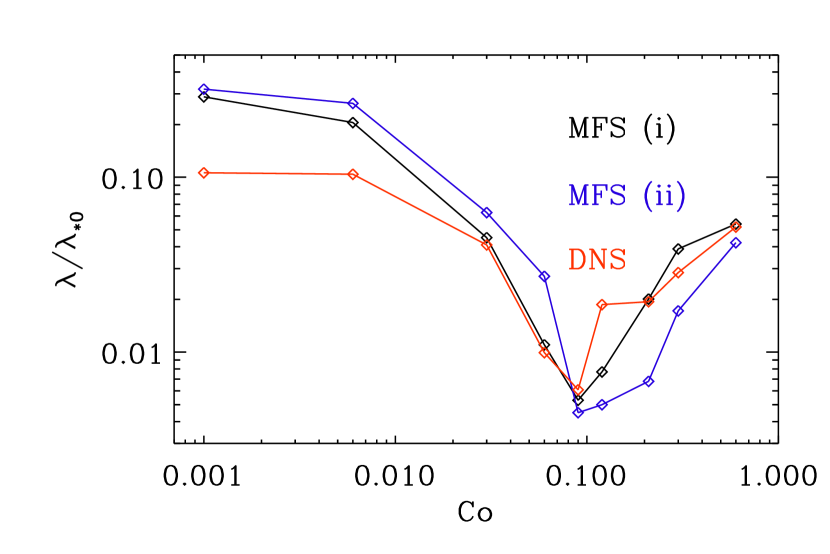
Figure 8: Non-dimensional growth rate of NEMPI versus Co for MFS(i) with $\beta_{\star}=0.33$ and MFS(ii) with $\beta_{\star}=0.44$, as well as DNS for $\mbox{\rm Gr}=0.033$ and $\beta_{0}=0.05$.

Owing to the effects of turbulent diffusion, the actual value of the growth rate of NEMPI is always expected to be less than $\lambda_{*0}$. Kemel et al. (2013) proposed an empirical formula replacing $\lambda$ by $\lambda+\eta_{\rm t}k^{2}$, where $k$ is the wavenumber. This would lead to

$$\lambda/\lambda_{*0}\propto 1-\mbox{\rm Gr}_{*}/\mbox{\rm Gr},$$ (36)

with a coefficient $\mbox{\rm Gr}_{*}=\tilde{\eta}_{\rm t}/3\beta_{\star}\mbox{\rm Ma}$. However, as we will see below, this expression is not found to be consistent with our numerical data.

The onset of the dynamo instability is governed by the dynamo number

$$C_{\alpha}=\epsilon_{\rm f0}\,\mbox{\rm Gr}\,\mbox{\rm Co}\,k_{\rm f}/k_{1}.$$ (37)

For a cubic domain, large-scale dynamo action occurs for $C_{\alpha}>1$, which was confirmed by Losada et al. (2013), who found the typical Beltrami fields for two supercritical cases. They used the parameters $\mbox{\rm Gr}=0.033$ and values of Co up to 0.6. Here we present MFS in two- and three-dimensional domains for the same values of Gr and a similar range of Co values. In Fig. 8, we compare the DNS of Losada et al. (2013) with our reference model defined through Eq. (30) and referred to as MFS(i) as well as with the case $\beta_{\star}=0.44$, referred to as MFS(ii).

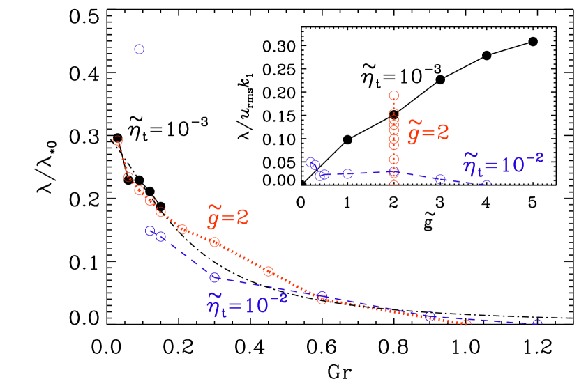
Figure 9: Normalized growth rate of NEMPI versus stratification parameter Gr that varies with changing gravity, $g$, for $\mbox{\rm Co}=0$ with constant $\tilde{\eta}_{\rm t}$ ($\tilde{\eta}_{\rm t}=10^{-3}$ black filled symbols and $\tilde{\eta}_{\rm t}=10^{-2}$ blue open symbols), or with changing $\eta_{\rm t}=\nu_{\rm t}$ for constant $\tilde{g}=2$ (red open symbols). The dash-dotted line shows the approximate fit given by Eq. (40). The inset shows the growth rate normalized by the turnover time as a function of $\tilde{g}$.

3.3 Larger stratification, smaller scale separation

The expected theoretical maximum growth rate of NEMPI is given by Eq. (35). At zero rotation, we thus expect $\lambda/\lambda_{*0}\approx 1$. To check this, we performed two-dimensional MFS in a squared domain of size $(2\pi)^{2}$. The result is shown in Fig. 9 for the model parameters given in Eq. (30). When Gr is small, we find that $\lambda/\lambda_{*0}\approx 0.3$, which is below the expected value. As we increase Gr, $\lambda/\lambda_{*0}$ decreases until NEMPI can no longer be detected for $\mbox{\rm Gr}\mathrel{\mathchoice{\vbox{\offinterlineskip\halign{\hfil$\displaystyle#$\hfil\cr>\cr\sim\cr}}}{\vbox{\offinterlineskip\halign{\hfil$\textstyle#$\hfil\cr>\cr\sim\cr}}}{\vbox{\offinterlineskip\halign{\hfil$\scriptstyle#$\hfil\cr>\cr\sim\cr}}}{\vbox{\offinterlineskip\halign{\hfil$\scriptscriptstyle#$\hfil\cr>\cr\sim\cr}}}}1.2$.

It is conceivable that this decrease may have been caused by the following two factors. First, the growth rate is expected to increase with Gr, but for fixed scale separation, the resulting density contrast becomes huge. Finite resolution might therefore have caused inaccuracies. Second, although the growth rate should not depend on $B_{0}$ (Kemel et al., 2012a), we need to make sure that the mode is fully contained within the domain. In other words, we are interested in the largest growth rate as we vary the value of $B_{0}$. Again, to limit computational expense, we tried only a small number of runs, keeping the size of the domain the same. This may have caused additional uncertainties. However, it turns out that our results are independent of whether Gr is changed by changing $g$ or $\eta_{\rm t}$ ($=\nu_{\rm t}$). This suggests that our results for large values of $g$ shown in Fig. 9 may in fact be accurate. To illustrate this more clearly, we rewrite

$$\mbox{\rm Gr}={3\eta_{\rm t}\over u_{\rm rms}H_{\rho}}={3\tilde{\eta}_{\rm t}\over k_{1}}\,{c_{\rm s}\over u_{\rm rms}}\,{g\over c_{\rm s}^{2}}=3\tilde{\eta}_{\rm t}\tilde{g}/\mbox{\rm Ma},$$ (38)

where we have defined

$$\tilde{\eta}_{\rm t}=\eta_{\rm t}k_{1}/c_{\rm s},\quad\tilde{g}=g/c_{\rm s}^{2}k_{1}\equiv(k_{1}H_{\rho})^{-1}.$$ (39)

Figure 9 shows that $\lambda/\lambda_{*0}$ is indeed independent of the individual values of $\tilde{\eta}_{\rm t}$ and $\tilde{g}$ as long as Gr is the same. For small values of $\tilde{g}$ and large diffusivity ($\tilde{\eta}_{\rm t}=10^{-2}$), the velocity evolves in an oscillatory fashion with a rapid growth and a gradual subsequent decline. In Fig. 9, the isolated data point at $\lambda/\lambda_{*0}\approx 0.44$ reflects the speed of growth during the periodic rise phase, but it is unclear whether or not it is related to NEMPI.

In the inset, we plot $\lambda/u_{\rm rms}k_{\rm f}$ versus $\tilde{g}$ itself. This shows that the growth rate (in units of the inverse turnover time) increases with increasing $\tilde{g}$ when $\tilde{\eta}_{\rm t}$ is small. However, as follows from theoretical analysis, the growth rate decreases with increasing $\tilde{\eta}_{\rm t}$. When $\tilde{\eta}_{\rm t}$ is larger (corresponding to smaller scale separation), the growth rate of NEMPI is reduced for the same value of $\tilde{g}$ and it decreases with $\tilde{g}$ when $\tilde{g}\mathrel{\mathchoice{\vbox{\offinterlineskip\halign{\hfil$\displaystyle#$\hfil\cr>\cr\sim\cr}}}{\vbox{\offinterlineskip\halign{\hfil$\textstyle#$\hfil\cr>\cr\sim\cr}}}{\vbox{\offinterlineskip\halign{\hfil$\scriptstyle#$\hfil\cr>\cr\sim\cr}}}{\vbox{\offinterlineskip\halign{\hfil$\scriptscriptstyle#$\hfil\cr>\cr\sim\cr}}}}2$.

The decrease of $\lambda/\lambda_{*0}$ with increasing values of Gr can be approximated by the formula

$$\lambda/\lambda_{*0}\approx 0.3\left/\left[1+2\mbox{\rm Gr}+(4\mbox{\rm Gr})^{2}\right]\right.,$$ (40)

which is shown in Fig. 9 as a dash-dotted line. This expression is qualitatively different from the earlier, more heuristic expression proposed by Kemel et al. (2013) where the dimensional growth rate was simply modified by an ad hoc diffusion term of the form $\eta_{\rm t}k^{2}$. In that case, contrary to our MFS, the normalized growth rate would actually increase with increasing values of Gr (see Eq. (36)).

3.4 Co dependence at larger stratification

We consider the normalized growth rate of the combined NEMPI and dynamo instabilities as a function of Co for different values of Gr. As is clear from Fig. 9, using a fixed value of $g$ and varying $\eta_{\rm t}$ gives us the possibility to increase Gr to larger values of up to 1. In the following we use this procedure to compare the behavior of the growth rate versus Co for three values of Gr, $0.12$, $0.21$, and $1$ (see Fig. 10). It can be seen that the behavior of the curves is independent of the values of Gr, but the points where the minima of the curves occur moves toward bigger values of Co as Gr increases. This also happens in the case when there is only dynamo action without imposed magnetic field (dashed lines in Fig. 10). One also sees that the increase of the growth rate with increasing Co is much stronger in the case of larger Gr (compare the lines for $\mbox{\rm Gr}=0.12$ with those for 0.21 and 1). Finally, comparing runs with and without imposed magnetic field, but the same value of Gr, the growth rate of NEMPI is in most cases below that of the coupled system with NEMPI and dynamo instability.

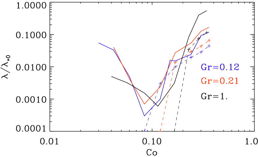
Figure 10: Normalized growth rate of the combined NEMPI and dynamo instability (solid lines) together with cases with pure dynamo instability (no imposed field, dashed lines) versus Co for three different values of Gr; $\mbox{\rm Gr}=0.12$ (blue), $\mbox{\rm Gr}=0.21$ (red), and $\mbox{\rm Gr}=1.0$ (black). In these simulations $\tilde{g}=4$ and $\tilde{\eta}_{\rm t}=10^{-3}$ (blue line), $\tilde{g}=3.5$, $\tilde{\eta}_{\rm t}=2\times 10^{-3}$ (red line), and $\tilde{g}=3.5$, $\tilde{\eta}_{\rm t}=9.5\times 10^{-3}$ (black line).

In Fig. 10 we see that the dependence of $\lambda/\lambda_{*0}$ on Gr is opposite for small and large values of Co. When $\mbox{\rm Co}\mathrel{\mathchoice{\vbox{\offinterlineskip\halign{\hfil$\displaystyle#$\hfil\cr<\cr\sim\cr}}}{\vbox{\offinterlineskip\halign{\hfil$\textstyle#$\hfil\cr<\cr\sim\cr}}}{\vbox{\offinterlineskip\halign{\hfil$\scriptstyle#$\hfil\cr<\cr\sim\cr}}}{\vbox{\offinterlineskip\halign{\hfil$\scriptscriptstyle#$\hfil\cr<\cr\sim\cr}}}}0.05$, an increase in Gr leads to a decrease in $\lambda/\lambda_{*0}$ (compare the $\mbox{\rm Gr}=1$ line with that for 0.21 along a cut through $\mbox{\rm Co}=0.05$ in Fig. 10), while for $\mbox{\rm Co}\mathrel{\mathchoice{\vbox{\offinterlineskip\halign{\hfil$\displaystyle#$\hfil\cr>\cr\sim\cr}}}{\vbox{\offinterlineskip\halign{\hfil$\textstyle#$\hfil\cr>\cr\sim\cr}}}{\vbox{\offinterlineskip\halign{\hfil$\scriptstyle#$\hfil\cr>\cr\sim\cr}}}{\vbox{\offinterlineskip\halign{\hfil$\scriptscriptstyle#$\hfil\cr>\cr\sim\cr}}}}0.2$, an increase in Gr leads to an increase in $\lambda/\lambda_{*0}$ (compare all three lines in Fig. 10 along a cut through $\mbox{\rm Co}=0.3$). The second case is caused by the increase of the dynamo number $C_{\alpha}$, which is directly proportional to Gr (see Eq. (37)). On the other hand, for small values of Co, only NEMPI operates, but if Gr in Eq. (38) is increased by increasing $\tilde{\eta}_{\rm t}$ rather than $\tilde{g}$, the dynamo is suppressed by enhanced turbulent diffusion (see also Fig. 9). This is related to the fact that the properties of the system depend not just on Gr and Co, but also on $k_{\rm f}/k_{1}$ or $C_{\alpha}$, which is proportional to all three parameters (see Eq. (37)).

4 Discussion and conclusions

The present work has brought us one step closer to being able to determine whether the observable solar activity such as sunspots and active regions could be the result of surface effects associated with strong stratification. A particularly important aspect has been the interaction with a dynamo process that must ultimately be responsible for generating the overall magnetic field. Recent global convective dynamo simulations of Nelson et al. (2011, 2013, 2014) have demonstrated that flux tubes with $\approx 40\,{\rm kG}$ field strength can be produced in the solar convection zone. This is almost as strong as the $\approx 100\,{\rm kG}$ magnetic flux tubes anticipated from earlier investigations of rising flux tubes requiring them to not break up and to preserve their east–west orientation (D’Silva & Choudhuri, 1993). Would we then still need surface effects such as NEMPI to produce sunspots? The answer might well be yes, because the flux ropes that have been isolated in the visualizations of Nelson et al. (2011, 2013, 2014) appear to have cross sections that are much larger than sunspots at the solar surface. Further concentration into thinner tubes would be required if they were to explain sunspots by just letting them pierce the surface.

Realistic hydromagnetic simulations of the solar surface are now beginning to demonstrate that $\approx 10\,{\rm kG}$ fields at a depth of $\approx 10\,{\rm Mm}$ can produce sunspot-like appearances at the surface (Rempel & Cheung, 2014). However, we have to ask about the physical process contributing to this phenomenon. A purely descriptive analysis of simulation data cannot replace the need for a more prognostic approach that tries to reproduce the essential physics using simpler models. Although Rempel & Cheung (2014) propose a mechanism involving mean-field terms in the induction equation, they do not show that their model equations can actually describe the process of magnetic flux concentration. In fact, their description is somewhat reminiscent of flux expulsion, which was invoked earlier by Tao et al. (1998) to explain the segregation of magneto-convection into magnetized and unmagnetized regions. In this context, NEMPI provides such an approach that can be used prognostically rather than diagnostically. However, this approach has problems of its own, some of which are addressed in the present work. Does NEMPI stop working when $\mbox{\rm Co}\mathrel{\mathchoice{\vbox{\offinterlineskip\halign{\hfil$\displaystyle#$\hfil\cr>\cr\sim\cr}}}{\vbox{\offinterlineskip\halign{\hfil$\textstyle#$\hfil\cr>\cr\sim\cr}}}{\vbox{\offinterlineskip\halign{\hfil$\scriptstyle#$\hfil\cr>\cr\sim\cr}}}{\vbox{\offinterlineskip\halign{\hfil$\scriptscriptstyle#$\hfil\cr>\cr\sim\cr}}}}0.03$? How does it interact with the underlying dynamo? Such a dynamo is believed to control the overall sunspot number and the concentration of sunspots to low latitudes.

Our new DNS suggest that, although rotation tends to suppress NEMPI, magnetic flux concentrations can still form at Coriolis numbers of $\mbox{\rm Co}\approx 0.1$. This is slightly larger than what was previously found from MFS both with horizontal and vertical magnetic fields and the same value of Gr. For the solar rotation rate of $\Omega\approx 3\times 10^{-6}\,{\rm s}^{-1}$, a value of $\mbox{\rm Co}\equiv 2\Omega\tau=0.1$ corresponds to $\tau=5\,{\rm h}$, which is longer than the earlier MFS values of $2\,{\rm h}$ for a horizontal field (Losada et al., 2013) and $30\min$ for a vertical field (Brandenburg et al., 2014).

Using the TFM, we have confirmed earlier findings regarding $\alpha$ and $\eta_{\rm t}$, although for our new simulations both coefficients are somewhat larger, which is presumably due to the larger scale separation. The ratio between $\alpha$ and $\eta_{\rm t}$ determines the dynamo number and is now about 40% below previous estimates. There is no evidence of other important mean-field effects that could change our conclusion about a cross-over from suppressed NEMPI to increased dynamo activity. We now confirm quantitatively that the enhanced growth past the initial suppression of NEMPI is indeed caused by mean-field dynamo action in the presence of a weak magnetic field. The position of the minimum in the growth rate coincides with the onset of mean-field dynamo action that takes the $\alpha$ effect into account.

For weak or no rotation, we find that the normalized NEMPI growth rate is described by a single parameter Gr, which is proportional to the product of gravity and turbulent diffusivity, where the latter is a measure of the inverse scale separation ratio. This normalization takes into account that the growth rate increases with increasing gravity. The growth rate compensated in this way shows a decrease with increasing gravity and turbulent diffusivity that is different from an earlier, more heuristic, expression proposed by Kemel et al. (2013). The reason for this departure is not quite clear. One possibility is some kind of gravitational quenching, because the suppression is well described by a quenching factor that becomes important when Gr exceeds a value of around 0.5. This quenching is probably not important for stellar convection where the estimated value of Gr is 0.17 (Losada et al., 2013). It might, however, help explain mismatches with the expected theoretical growth rate that was found to be proportional to Gr (Kemel et al., 2013) and that was determined from recent DNS (Brandenburg et al., 2014).

An important question is whether NEMPI will really be strong enough to produce sunspots with super-equipartition strength. It has always been clear that NEMPI can only work for a magnetic field strength that is a small fraction of the local equipartition field value. However, super-equipartition fields are produced if the magnetic field is vertical (Brandenburg et al., 2013). Subsequent work showed quantitatively that NEMPI does indeed work at subequipartition field strengths, but since mass flows mainly along magnetic field lines, the reduced pressure leads to suction which tends to evacuate the upper parts of the tube (Brandenburg et al., 2014). This is similar to the “hydraulic effect” envisaged by Parker (1976), who predicted such downflows along flux tubes. In a later paper Parker (1978), gives more realistic estimates, but the source of downward flows remained unclear. Meanwhile, the flux emergence simulations of Rempel & Cheung (2014) show at first upflows in their magnetic spots (see their Fig. 5), but as the spots mature, a downflow develops (see their Fig. 7). In their case, because they have convection, those downflows can also be ascribed to supergranular downflows, as was done by Stein & Nordlund (2012). Nevertheless, in the isothermal simulations of Brandenburg et al. (2013, 2014), this explanation would not apply. Thus, we now know that the required downflows can be caused by NEMPI, but we do not know whether this is also what happens in the Sun.

Coming back to our paper, where NEMPI is coupled to a dynamo, the recent work of Mitra et al. (2014) is relevant because it shows that intense bipolar spots can be generated in an isothermal simulation with strongly stratified non-helically driven turbulence in the upper part and a helical dynamo in the lower part. The resulting surface structure resembles so-called $\delta$ spots that have previously only been found in the presence of strongly twisted and kink-unstable flux tubes (Linton et al., 1998). While the detailed mechanism of this work is not yet understood, it reminds us that it is too early to draw strong conclusions about NEMPI as long as not all its aspects have been explored in sufficient detail.