Maximizing Energy-Efficiency in Multi-Relay OFDMA Cellular Networks

Abstract

This contribution presents a method of obtaining the optimal power and subcarrier allocations that maximize the energy-efficiency (EE) of a multi-user, multi-relay, orthogonal frequency division multiple access (OFDMA) cellular network. Initially, the objective function (OF) is formulated as the ratio of the spectral-efficiency (SE) over the power consumption of the network. This OF is shown to be quasi-concave, thus Dinkelbach’s method can be employed for solving it as a series of parameterized concave problems. We characterize the performance of the aforementioned method by comparing the optimal solutions obtained to those found using an exhaustive search. Additionally, we explore the relationship between the achievable SE and EE in the cellular network upon increasing the number of active users. In general, increasing the number of users supported by the system benefits both the SE and EE, and higher SE values may be obtained at the cost of EE, when an increased power may be allocated.

I Introduction

In recent years, increasing the energy-efficiency (EE) of cellular networks has become an important design metric in the telecommunications community, especially in the light of the conflicting criteria of achieving both an increased data rate as well as reducing the ’carbon footprint’. Consequently, joint academic and industrial effort has been dedicated to developing novel energy-saving techniques for next-generation networks [1]. This contribution considers the downlink (DL) EE maximization (EEM) problem in a multi-user, multi-relay, orthogonal frequency division multiple access (OFDMA) network such as that specified both in the third generation partnership project’s (3GPP) long term evolution-advanced (LTE-A) and in the IEEE 802.16 worldwide interoperability for microwave access (WiMAX) standards.

Numerous contributions have already dealt with the problem of allocating power and/or subcarriers in an OFDMA network with the goal of either spectral-efficiency (SE) maximization [2], or power minimization subject to specific quality-of-service (QoS) constraints [3, 4]. However, these works have not solved the EEM problem, which has only recently become the center of attention in the community. In fact, the EEM problem can be viewed as an example of multi-objective optimization, since typically the goal is to maximize the SE achieved, while concurrently minimizing the power consumption. Hence the authors of [5] derived an aggregate OF, which consists of a weighted sum of the SE achieved and the total power dissipated. However, selecting appropriate weights for the two OFs is not trivial, and different combinations of weights can lead to different results. Another example is given in [6], where the EEM problem is considered in a multi-relay network. Nonetheless, both [5, 6] only optimize the user selection and power allocation without considering the subcarrier allocation in the network. Another formulation was advocated in [7], which considers the power and subcarrier allocation problem in an OFDMA cellular network, but without a maximum total power constraint and without relaying. The authors of [8] formulated the EEM problem in a OFDMA cellular network under a maximum total power constraint, but relaying was not considered.

In contrast to the aforementioned related work, this contribution focuses on jointly optimizing both the power and subcarrier allocation for a multi-relay, multi-user OFDMA cellular network, while considering a specific maximum total power constraint. As a benefit of its low-complexity implementation, we employ the amplify-and-forward (AF) [9] protocol at the relays. The contributions of this paper are summarized as follows.

The EEM problem, in the context of a multi-relay, multi-user OFDMA cellular network, in which both direct and relayed transmissions are employed, is formulated as a fractional programming problem, which jointly considers both the power and the subcarrier allocation under a maximum power constraint. This problem is relaxed and can be shown to be quasi-concave, therefore Dinkelbach’s method [10] may be employed for iteratively obtaining the optimal solution. It is demonstrated that the EEM algorithm reaches the optimal solution within a low number of iterations and succeeds in reaching the solution obtained via an exhaustive search. Thus the original problem is solved at a low complexity.

Furthermore, comparisons are made between the EEM and the SE maximization (SEM) based solutions. As an example, it is shown that when the maximum affordable power is lower than a given threshold, the two problems have the same solutions. However, as the maximum affordable power is increased, the SEM algorithm attempts to achieve a higher SE at the cost of a lower EE. By contrast, given the total power, the EEM algorithm reaches the upper limit of the maximum achievable SE for the sake of maintaining the maximum EE. Additionally, we will demonstrate that both the SE and EE benefit from an increased multi-user diversity in the network.

II System Model

We consider an OFDMA DL cellular system consisting of a single base station (BS), $M$ fixed relay nodes (RNs) and $K$ uniformly-distributed user-equipment (UEs), as shown in Fig. 1. This network has access to $N$ subcarriers, and the cell is partitioned into $M$ sectors such that the UEs in each sector are served by the single RN. In order to reduce the detrimental effect of path-loss on the achievable SE and EE, each UE may only be served by the specific RN that it is closest to, and thus RN selection is implicitly accomplished. The BS may perform DL transmissions either via a direct BS-to-UE link, or by relying on the RN for creating an AF BS-to-RN-to-UE link. Additionally, we assume that the total available instantaneous transmission power of the network is $P_{max}$. Below, we adopt the following notation. The variables related to the two possible communication protocols are denoted by the superscripts $D$ and $A$, respectively. When defining links, the subscript $0$ is used for indicating the BS, while $\mathcal{M}(k)\in\{1,\cdots,M\}$ indicates the RN selected for assisting the DL-transmissions to user $k$.

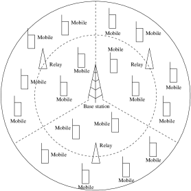
Figure 1: An example of a cellular network with $M=3$ RNs and $K=18$ UEs.

The attained SE when using the direct and relayed transmissions [9] may be expressed as

$$R_{k}^{D,n}(\mathcal{P})=\mbox{log}_{2}\left(1+\frac{P_{0,k}^{D,n}G_{0,k}^{n}}{\Delta\gamma N_{0}W}\right)\mbox{ }\mbox{[bits/s/Hz]}$$ (1)

and (2), respectively.

$$R_{k}^{A,n}(\mathcal{P})\approx\frac{1}{2}\mbox{log}_{2}\left(1+\frac{P_{0,\mathcal{M}(k)}^{A,n}G_{0,\mathcal{M}(k)}^{n}P_{\mathcal{M}(k),k}^{A,n}G_{\mathcal{M}(k),k}^{n}}{\Delta\gamma N_{0}W\left(P_{0,\mathcal{M}(k)}^{A,n}G_{0,\mathcal{M}(k)}^{n}+P_{\mathcal{M}(k),k}^{A,n}G_{\mathcal{M}(k),k}^{n}\right)}\right)\mbox{ }\mbox{[bits/s/Hz]},$$ (2)

To elaborate, $P_{a,b}^{X,n}$ is the power allocated to transmitter $a\in\{0,\cdots,M\}$ using protocol $X\in\{D,A\}$ for transmission to receiver $b$ on subcarrier $n$. Furthermore, $G_{a,b}^{n}$ represents the channel’s attenuation between transmitter $a$ and receiver $b$ on subcarrier $n$, which is assumed to be known at the BS for all links, $N_{0}$ is the additive white Gaussian noise (AWGN) variance and $W$ is the bandwidth of a single subcarrier. The signal-to-noise (SNR) gap, $\Delta\gamma$, is measured at the system’s bit error ratio (BER) target, and is the difference between the SNR required at the discrete-input continuous-output memoryless channel (DCMC) capacity and the actual SNR required the modulation and coding schemes of the practical physical layer transceivers employed. In Section V, we make the simplifying assumption that idealized transceivers operating exactly at the DCMC capacity are employed, thus $\Delta\gamma=0\mbox{ dB}$. Additionally, the power allocation policy of the system is denoted by $\mathcal{P}$, which determines the values of $P_{a,b}^{X,n}$. The factor of $\frac{1}{2}$ in (2) accounts for the fact that only half the transmission time is available for transmitting new data, while the other half must be used for the AF relaying. Additionally, high receiver’s SNR values is assumed in (2), which is valid for $P_{0,\mathcal{M}(k)}^{A,n}G_{0,\mathcal{M}(k)}^{n}+P_{\mathcal{M}(k),k}^{A,n}G_{\mathcal{M}(k),k}^{n}\gg\Delta\gamma N_{0}W$.

The subcarrier indicator variable $s_{k}^{X,n}\in\{0,1\}$ is now introduced, which denotes the allocation of subcarrier $n$ for transmission to user $k$ using protocol $X$ when $s_{k}^{X,n}=1$, and $s_{k}^{X,n}=0$ otherwise. The average SE of the system is then calculated as

$$R_{T}(\mathcal{P},\mathcal{S})=\frac{1}{N}\sum_{k=1}^{K}\sum_{n=1}^{N}s_{k}^{D,n}R_{k}^{D,n}+\frac{s_{k}^{A,n}}{2}R_{k}^{A,n}\mbox{\mbox{ }[bits/s/Hz]},$$ (3)

where $\mathcal{S}$ denotes the subcarrier allocation policy of the system, which determines the values of the subcarrier indicator variable $s_{k}^{X,n}$.

In order to compute the energy used in these transmissions, a model similar to [11] is adopted where the total power consumption of the system is assumed be governed by a constant term and a term that varies with the transmission powers, which may be written as (4).

$$P_{T}(\mathcal{P},\mathcal{S})=\left(P_{C}^{(B)}+M\cdot P_{C}^{(R)}\right)+\sum_{k=1}^{K}\sum_{n=1}^{N}s_{k}^{D,n}\xi^{(B)}P_{0,k}^{D,n}+\frac{1}{2}s_{k}^{A,n}\cdot\left(\xi^{(B)}P_{0,\mathcal{M}(k)}^{A,n}+\xi^{(R)}P_{\mathcal{M}(k),k}^{A,n}\right)\mbox{ }\mbox{[Watts]}$$ (4)

Here, $P_{C}^{(B)}$ and $P_{C}^{(R)}$ represent the fixed power consumption of each BS and each RN, respectively, while $\xi^{(B)}>1$ and $\xi^{(R)}>1$ denote the reciprocal of the drain efficiencies of the power amplifiers employed at the BS and the RNs, respectively. For example, an amplifier having a $25\%$ drain efficiency would have $\xi=\frac{1}{0.25}=4$.

Finally, the average EE metric of the system is expressed as

$$\eta_{E}(\mathcal{P},\mathcal{S})=\frac{R_{T}(\mathcal{P},\mathcal{S})}{P_{T}(\mathcal{P},\mathcal{S})}\mbox{ [bits/Joule/Hz]}.$$ (5)

III Problem Formulation

The aim of this work is to maximize the EE metric of (5) subject to a maximum total instantaneous transmit power constraint. In its current form, (5) is dependent on $3KN$ continuous power variables $P_{0,k}^{D,n}$, $P_{0,\mathcal{M}(k)}^{A,n}$ and $P_{\mathcal{M}(k),k}^{A,n}$, $\forall k,n$, and $2KN$ binary subcarrier indicator variables $s_{k}^{D,n}$ and $s_{k}^{A,n}$, $\forall k,n$. Thus, it may be regarded as a MINLP problem, and can be solved using the branch-and-bound method [12]. However, the computational effort required for branch-and-bound techniques typically increases exponentially with the problem size. Therefore, a simpler solution is derived by relaxing the binary constraint imposed on the subcarrier indicator variables, $s_{k}^{D,n}$ and $s_{k}^{A,n}$, so that they may assume continuous values from the interval $[0,1]$, as demonstrated in [3, 13]. Furthermore, the auxiliary variables $\widetilde{P}_{0,k}^{D,n}=P_{0,k}^{D,n}s_{k}^{D,n}$, $\widetilde{P}_{0,\mathcal{M}(k)}^{A,n}=P_{0,\mathcal{M}(k)}^{A,n}s_{k}^{A,n}$ and $\widetilde{P}_{0,\mathcal{M}(k)}^{A,n}=P_{0,\mathcal{M}(k)}^{A,n}s_{k}^{A,n}$ are introduced.

The relaxation of the binary constraints imposed on the variables $s_{k}^{D,n}$ and $s_{k}^{A,n}$ allows them to assume continuous values, which leads to a time-sharing subcarrier allocation between the UEs. Naturally, the original problem is not actually solved. However, it has been shown that solving the dual of the relaxed problem provides solutions that are arbitrarily close to the original, non-relaxed problem, provided that the number of available subcarriers tends to infinity [13]. It has empirically been shown that in some cases only $8$ subcarriers are required for obtaining close-to-optimal results [14]. It shall be demonstrated in Section V that even for as few as two subcarriers, the solution algorithm employed in this work approaches the optimal EE achieved by an exhaustive search.

The optimization problem is formulated as shown as follows.

Relaxed Problem (P):

$$\underset{\mathcal{P},\mathcal{S}}{\mbox{maximize}} \frac{\widetilde{R}_{T}}{\widetilde{P}_{T}}$$ (6)

subject to $$\sum_{k=1}^{K}\sum_{n=1}^{N}\widetilde{P}_{0,k}^{D,n}+\widetilde{P}_{0,\mathcal{M}(k)}^{A,n}+\widetilde{P}_{\mathcal{M}(k),k}^{A,n}\leq P_{max},$$ (11)

$$s_{k}^{D,n}+s_{k}^{A,n}\leq 1\mbox{, }\forall k,n,$$

$$\sum_{k=1}^{K}s_{k}^{D,n}+s_{k}^{A,n}\leq 1\mbox{, }\forall n,$$

$$\widetilde{P}_{0,k}^{D,n}\mbox{, }\widetilde{P}_{0,\mathcal{M}(k)}^{A,n}\mbox{, }\widetilde{P}_{\mathcal{M}(k),k}^{A,n}\in\mathbb{R}_{+}\mbox{, }\forall k,n,$$

$$0\leq s_{k}^{D,n}\mbox{, }s_{k}^{A,n}\leq 1\mbox{, }\forall k,n,$$

where the objective function is the ratio between (12) and (13).

$$\widetilde{R}_{T} = \sum_{k=1}^{K}\sum_{n=1}^{N}s_{k}^{D,n}\mbox{log}_{2}\left(1+\frac{\widetilde{P}_{0,k}^{D,n}G_{0,k}^{n}}{s_{k}^{D,n}\Delta\gamma N_{0}W}\right)$$ (12)

$$+\frac{s_{k}^{A,n}}{2}\mbox{log}_{2}\left(1+\frac{\widetilde{P}_{0,\mathcal{M}(k)}^{A,n}G_{0,\mathcal{M}(k)}^{n}\widetilde{P}_{\mathcal{M}(k),k}^{A,n}G_{\mathcal{M}(k),k}^{n}}{s_{k}^{A,n}\Delta\gamma N_{0}W\left(\widetilde{P}_{0,\mathcal{M}(k)}^{A,n}G_{0,\mathcal{M}(k)}^{n}+\widetilde{P}_{\mathcal{M}(k),k}^{A,n}G_{\mathcal{M}(k),k}^{n}\right)}\right)$$

$$\widetilde{P}_{T}=\left(P_{C}^{(B)}+M\cdot P_{C}^{(R)}\right)+\sum_{k=1}^{K}\sum_{n=1}^{N}\xi^{(B)}\widetilde{P}_{0,k}^{D,n}+\frac{1}{2}\left(\xi^{(B)}\widetilde{P}_{0,\mathcal{M}(k)}^{A,n}+\xi^{(R)}\widetilde{P}_{\mathcal{M}(k),k}^{A,n}\right)$$ (13)

In this formulation, the variables to be optimized are $s_{k}^{D,n}$, $s_{k}^{A,n}$, $\widetilde{P}_{0,k}^{D,n}$, $\widetilde{P}_{0,\mathcal{M}(k)}^{A,n}$ and $\widetilde{P}_{\mathcal{M}(k),k}^{A,n}$, $\forall k,n$. Physically, the constraint (LABEL:eq:C1) ensures that the sum of the power allocated to variables $\widetilde{P}_{0,k}^{D,n}$, $\widetilde{P}_{0,\mathcal{M}(k)}^{A,n}$ and $\widetilde{P}_{\mathcal{M}(k),k}^{A,n}$ does not exceed the maximum power budget of the system. Constraint (11) ensures that a single transmission protocol, either direct or AF, is chosen for each user-subcarrier pair. The constraint (11) guarantees that each subcarrier is only allocated to at most one user, thus intra-cell interference is avoided. The constraints (11) and (11) describe the feasible region of the optimization variables. The OF of problem (P) is quasi-concave [10], please see [15] for the proof.

IV Dinkelbach’s method for solving the problem (P)

Dinkelbach’s method [10] is an iterative algorithm that can be used for solving a quasi-concave problem in a parameterized concave form. The value of the parameter at iteration $i$ is denoted by $q_{i}$, and the parameterized form is given by

Subtractive problem (P^′):

$$\underset{\mathcal{P},\mathcal{S}}{\mbox{maximize}} \widetilde{R}_{T}(\mathcal{P},\mathcal{S})-q_{i}\widetilde{P}_{T}(\mathcal{P},\mathcal{S})$$ (14)

subject to $$(\ref{eq:C1}),(\ref{eq:C2}),(\ref{eq:C3}),(\ref{eq:C4}),(\ref{eq:C5}),$$

which is solved at each iteration for obtaining an updated parameter value. For futher details, please refer to [10].

Since $\widetilde{R}_{T}(\mathcal{P},\mathcal{S})$ and $\widetilde{P}_{T}(\mathcal{P},\mathcal{S})$ are concave and affine, respectively [15], it is plausible that the OF in (P^′) is concave. Thus, (P^′) is a typical concave maximization problem and may be solved using convex optimization techniques. In this work, we opt for the method of dual decomposition [16], which solves (P^′) by solving a series of subproblems. This approach is favorable in this context as the OF in (P^′) is formed by the summation of multiple similar terms of separate variables, where the maximization of each term can be solved in a parallel fashion using a decomposition technique. Let us commence by stating that the Lagrangian of (P^′) is given by (15),

$$\mathcal{L}\left(\mathcal{P},\mathcal{S},\lambda\right) = \widetilde{R}_{T}(\mathcal{P},\mathcal{S})-q_{i}\widetilde{P}_{T}(\mathcal{P},\mathcal{S})+\lambda\left(P_{max}-\sum_{k=1}^{K}\sum_{n=1}^{N}\widetilde{P}_{0,k}^{D,n}+\widetilde{P}_{0,\mathcal{M}(k)}^{A,n}+\widetilde{P}_{\mathcal{M}(k),k}^{A,n}\right).$$ (15)

where $\lambda\geq 0$ is the Lagrangian multiplier associated with the constraint (LABEL:eq:C1). The feasible region constraints (11) and (11), as well as constraints (11) and (11) will be considered, when deriving the optimal solution, which is detailed later.

The dual problem of (P^′) may be written as [16] $\underset{\lambda\geq 0}{\mbox{min.}}\mbox{ }g(\lambda)=\underset{\lambda\geq 0}{\mbox{min.}}\mbox{ }\underset{\mathcal{P},\mathcal{S}}{\mbox{max.}}\mbox{ }\mathcal{L}\left(\mathcal{P},\mathcal{S},\lambda\right)$, which is solved by solving $NK$ similar subproblems for obtaining both the power as well as the subcarrier allocations, and by solving a master problem to update $\lambda$, until convergence is obtained.

IV-A Solving the $NK$ subproblems

These subproblems are solved by employing the Karush–Kuhn–Tucker (KKT) conditions [17], which are first-order necessary and sufficient conditions for optimality. We denote all optimal variables by a superscript asterisk, and the total transmit power assigned for AF transmission to user $k$ over subcarrier $n$ by $\widetilde{P}_{k}^{A,n}=\widetilde{P}_{0,\mathcal{M}(k)}^{A,n}+\widetilde{P}_{\mathcal{M}(k),k}^{A,n}$. Then, by substituting $\widetilde{P}_{\mathcal{M}(k),k}^{A,n}=\widetilde{P}_{k}^{A,n}-\widetilde{P}_{0,\mathcal{M}(k)}^{A,n}$ into (15), the following first-order derivatives may be obtained

$$\left.\frac{\partial\mathcal{L}\left(\mathcal{P},\mathcal{S},\lambda\right)}{\partial\widetilde{P}_{0,k}^{D,n}}\right|_{\widetilde{P}_{0,k}^{D,n}=\widetilde{P}_{0,k}^{D,n*}}=0,$$ (16)

$$\left.\frac{\partial\mathcal{L}\left(\mathcal{P},\mathcal{S},\lambda\right)}{\partial\widetilde{P}_{k}^{A,n}}\right|_{\widetilde{P}_{k}^{A,n}=\widetilde{P}_{k}^{A,n*}}=0$$ (17)

and

$$\left.\frac{\partial\mathcal{L}\left(\mathcal{P},\mathcal{S},\lambda\right)}{\partial\widetilde{P}_{0,\mathcal{M}(k)}^{A,n}}\right|_{\widetilde{P}_{0,\mathcal{M}(k)}^{A,n}=\widetilde{P}_{0,\mathcal{M}(k)}^{A,n*}}=0.$$ (18)

The optimal values of $\widetilde{P}_{0,k}^{D,n}$ may be readily obtained from (16) as

$$P_{0,k}^{D,n*}=\left[\frac{1}{\ln 2\left(q_{i}\xi^{(B)}+\lambda\right)}-\frac{1}{\alpha_{k}^{D,n}}\right]^{+},$$ (19)

where the effective channel gain of the direct transmission is given by $\alpha_{k}^{D,n}=\frac{G_{0,k}^{n}}{\Delta\gamma N_{0}W}$ and $[\cdot]^{+}$ denotes $\max(0,\cdot)$, since the powers allocated have to be nonnegative due to the constraint (11). Similarly the optimal values of $\widetilde{P}_{0,\mathcal{M}(k)}^{A,n}$ and $\widetilde{P}_{\mathcal{M}(k),k}^{A,n}$ may be obtained by equating (17) and (18) to give

$$P_{0,\mathcal{M}(k)}^{A,n*}=\beta_{k}^{A,n}P_{k}^{A,n*}$$ (20)

and

$$P_{\mathcal{M}(k),k}^{A,n*}=\left(1-\beta_{k}^{A,n}\right)P_{k}^{A,n*},$$ (21)

where the total transmit power assigned for the AF transmission to user $k$ over subcarrier $n$ is given by (22), (23) and (24).

$$P_{k}^{A,n*}=\left[\frac{1}{\ln 2\left(\beta_{k}^{A,n}\left(q_{i}\xi^{(B)}+2\lambda\right)+\left(1-\beta_{k}^{A,n}\right)\left(q_{i}\xi^{(R)}+2\lambda\right)\right)}-\frac{1}{\alpha_{k}^{A,n}}\right]^{+}$$ (22)

$$\alpha_{k}^{A,n}=\frac{\beta_{k}^{A,n}\left(1-\beta_{k}^{A,n}\right)G_{0,\mathcal{M}(k)}^{n}G_{\mathcal{M}(k),k}^{n}}{\left(\beta_{k}^{A,n}G_{0,\mathcal{M}(k)}^{n}+\left(1-\beta_{k}^{A,n}\right)G_{\mathcal{M}(k),k}^{n}\right)\Delta\gamma N_{0}W}$$ (23)

$$\beta_{k}^{A,n}=\frac{-G_{\mathcal{M}(k),k}^{n}\left(q_{i}\xi^{(R)}+2\lambda\right)+\sqrt{G_{0,\mathcal{M}(k)}^{n}G_{\mathcal{M}(k),k}^{n}\left(q_{i}\xi^{(B)}+2\lambda\right)\left(q_{i}\xi^{(R)}+2\lambda\right)}}{G_{0,\mathcal{M}(k)}^{n}\left(q_{i}\xi^{(B)}+2\lambda\right)-G_{\mathcal{M}(k),k}^{n}\left(q_{i}\xi^{(R)}+2\lambda\right)}$$ (24)

Observe that (24) is the fraction of the total AF transmit power that is allocated for the BS-to-RN link while obeying $0\leq\beta_{k}^{A,n}\leq 1$.

Having calculated the optimal power allocations, the optimal subcarrier allocations may be derived using the first-order derivatives as follows:

$$\frac{\partial\mathcal{L}\left(\mathcal{P},\mathcal{S},\lambda\right)}{\partial s_{k}^{D,n}} = \log_{2}\left(1+\alpha_{k}^{D,n}P_{0,k}^{D,n*}\right)$$ (25)

$$-\frac{\alpha_{k}^{D,n}P_{0,k}^{D,n*}}{\ln 2\left(1+\alpha_{k}^{D,n}P_{0,k}^{D,n*}\right)}$$

$$= D_{k}^{n}\begin{cases}<0&\mbox{if }s_{k}^{D,n*}=0,\\ =0&\mbox{if }s_{k}^{D,n*}\in(0,1)\\ >0&\mbox{if }s_{k}^{D,n*}=1\end{cases},$$

and

$$\frac{\partial\mathcal{L}\left(\mathcal{P},\mathcal{S},\lambda\right)}{\partial s_{k}^{A,n}} = \frac{1}{2}\log_{2}\left(1+\alpha_{k}^{A,n}\widetilde{P}_{k}^{A,n*}\right)$$ (26)

$$-\frac{\alpha_{k}^{A,n}\widetilde{P}_{k}^{A,n*}}{2\ln 2\left(1+\alpha_{k}^{A,n}\widetilde{P}_{k}^{A,n*}\right)}$$

$$= A_{k}^{n}\begin{cases}<0&\mbox{if }s_{k}^{A,n*}=0,\\ =0&\mbox{if }s_{k}^{A,n*}\in(0,1)\\ >0&\mbox{if }s_{k}^{A,n*}=1.\end{cases},$$ (27)

(25) and (27) stem from the fact that if the optimal value of $s_{k}^{X,n}$ occurs at the boundary of the feasible region, then $\mathcal{L}\left(\mathcal{P},\mathcal{S},\lambda\right)$ must be decreasing with the values of $s_{k}^{X,n}$ that approach the interior of the feasible region. By contrast, for example, the derivative $D_{k}^{n}=0$ if the optimal $s_{k}^{D,n}$ is obtained in the interior of the feasible region [3]. However, since each subcarrier may only be used for transmission to a single user, each subcarrier $n$ is allocated to the specific user $k$ having the highest value of $\max\left(A_{k}^{n},D_{k}^{n}\right)$ in order to achieve the highest increase in $\mathcal{L}\left(\mathcal{P},\mathcal{S},\lambda\right)$. The optimal allocation for subcarrier $n$ is as follows

$$s_{k}^{D,n*}=\left\{\begin{array}[]{cc}1,&\mbox{if }D_{k}^{n}=\max_{j}\left[\max\left(A_{j}^{n},D_{j}^{n}\right)\right]\mbox{ and }D_{k}^{n}\geq 0,\\ 0,&\mbox{otherwise,}\end{array}\right.$$ (28)

and

$$s_{k}^{A,n*}=\left\{\begin{array}[]{cc}1,&\mbox{if }A_{k}^{n}=\max_{j}\left[\max\left(A_{j}^{n},D_{j}^{n}\right)\right]\mbox{ and }A_{k}^{n}\geq 0,\\ 0,&\mbox{otherwise.}\end{array}\right.$$ (29)

Thus constraints (11)- (11) are satisfied and the optimal primal variables are obtained for a given $\lambda$. Observe that the optimal power allocations given by (19) and (22) are indeed customized water-filling solutions, where the effective channel gains are given by $\alpha_{k}^{D,n}$ and $\alpha_{k}^{A,n}$, respectively, and where the water levels are determined both by the cost of allocating power, $\lambda$, as well as the current cost of power to the EE given by $q_{i}$.

IV-B Updating the dual variable $\lambda$

Since (19), (20), (21), (28) and (29) give a unique solution for $\mbox{$\underset{\mathcal{P},\mathcal{S}}{\mbox{max.}}$ }\mathcal{L}\left(\mathcal{P},\mathcal{S},\lambda\right)$, it follows that $g(\lambda)$ is differentiable and hence the gradient method [17, 16] may be readily used for updating the dual variables $\lambda$. The gradient of $\lambda$ is given by

$$\frac{\partial\mathcal{L}\left(\mathcal{P},\mathcal{S},\lambda\right)}{\partial\lambda}=P_{max}-\sum_{k=1}^{K}\sum_{n=1}^{N}\Big{(}\widetilde{P}_{0,k}^{D,n}+\widetilde{P}_{0,\mathcal{M}(k)}^{A,n}+\widetilde{P}_{\mathcal{M}(k),k}^{A,n}\Big{)}.$$ (30)

Therefore, $\lambda$ may be updated using the optimal variables to give (31),

$$\lambda(i+1)=\left[\lambda(i)-\alpha_{\lambda}(i)\left(P_{max}-\sum_{k=1}^{K}\sum_{n=1}^{N}\widetilde{P}_{0,k}^{D,n*}+\widetilde{P}_{0,\mathcal{M}(k)}^{A,n*}+\widetilde{P}_{\mathcal{M}(k),k}^{A,n*}\right)\right]^{+}$$ (31)

where $\alpha_{\lambda}(i)$ is the size of the step taken in the direction of the negative gradient for the dual variable $\lambda$ at iteration $i$. For the performance investigations of Section V, a constant step size is used, since it is comparatively easier to find a value that strikes a balance between optimality and convergence speed. The process of computing the optimal power as well as subcarrier allocations and subsequently updating $\lambda$ is repeated until convergence is attained, indicating that the dual optimal point has been reached. Since the primal problem (P^′) is concave, there is zero duality gap between the dual and primal solutions. Hence, solving the dual problem is equivalent to solving the primal problem. For additional clarity, the solution methodology is summarized in Fig. 2.

Figure 2: Summary of the solution methodology for the relaxed problem (P).

V Numerical results and discussions

TABLE I: Simulation parameters used to obtain all results in this section unless otherwise specified.

Simulation parameter	Value
Subcarrier bandwidth, $W$ Hertz	$12$k
$P_{C}^{(B)}$ Watts [11]	60
$P_{C}^{(R)}$ Watts [11]	20
$\xi^{(B)}$ [11]	2.6
$\xi^{(R)}$ [11]	5
$N_{0}$ dBm/Hz	−174
Convergence tolerance	$10^{-8}$
Number of channel samples	$10^{4}$

This section presents the results of applying the EEM algorithm described in Section IV to the relay-aided cellular system shown in Fig. 1, where the RNs are placed halfway between the BS and the cell-edge. The channel is modeled by the path-loss [18] and uncorrelated Rayleigh fading obeying the complex normal distribution, $\mathcal{CN}(0,1)$. It is assumed that the BS-to-RN link has line-of-sight (LOS) propagation, implying that a RN was placed on a tall building. However, the BS-to-UE and RN-to-UE links typically have no LOS, since these links are likely to be blocked by buildings and other large obstructing objects. An independently-random set of UE locations as well as fading channel realizations are generated for each channel sample. For fair comparisons, the metrics used are the average SE per subcarrier and the average EE per subcarrier. On the other hand, the sum-rate may be calculated by multiplying the average SE by $NW.$ Additionally, $\rho$ is introduced to denote the average fraction of the total number of subcarriers that are used for AF transmission. Thus, $\rho$ quantifies the benefit attained from introducing RNs into the system.

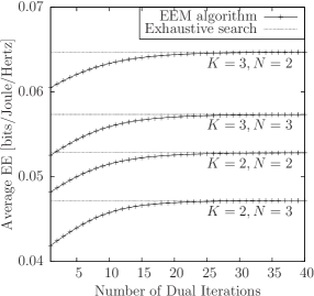
Figure 3: Average EE versus the total number of inner iterations of Dinkelbach’s method required for reaching convergence when using the simulation parameters from Table I with $P_{max}=0$dBm, $M=0$ and with a cell radius of $1$km.

Fig. 3 illustrates the convergence behavior of Dinkelbach’s method invoked for maximizing the EE for a selection of small-scale systems, averaged over $10^{4}$ different channel realizations. Since the problem size is small, it is possible to generate also the exhaustive-search based solution within a reasonable computation time. As seen in Fig. 3, Dinkelbach’s method converges to the optimal value within forty inner iterations. This result demonstrates that the EEM algorithm based on Dinkelbach’s method indeed obtains the optimal power and subcarrier allocation, even though the relaxed problem is solved and a high receiver’s SNR was assumed.

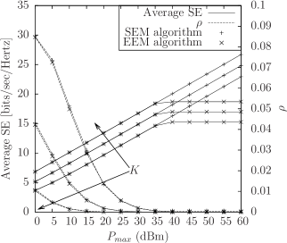
(a) Average SE and $\rho$ versus $P_{max}$ for $K=30$, $60$ and $120$.

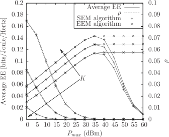
(b) Average EE and $\rho$ versus $P_{max}$ for $K=30$, $60$ and $120$.

Figure 4: Average SE, EE and $\rho$, and the effect of an increasing number of users, $K$, for a system with simulation parameters from Table I with $N=128$, $M=3$ and with a cell radius of $1.5$km.

Additionally, the EEM algorithm may be employed for evaluating the effects of system-level design choices on the network’s SE and EE. The effect of $K$ on the average EE and SE is depicted in Fig. 4. As expected, upon increasing $K$, the multi-user diversity of the system is increased, since the scheduler is allowed to choose its subcarrier allocations from a larger pool of channel gains. This results in an increase of both the maximum EE as well as of the SE attained. Furthermore, Fig. 4 shows that as $P_{max}$ is increased, the SEM algorithm continues to allocate more power in order to achieve a higher average SE at the cost of EE, while the EEM algorithm attains the maximum EE and does not continue to increase its attainable SE by sacrificing the achieved EE. On the other hand, $\rho$ is inversely proportional to $K$. This indicates that as the multi-user diversity increases, the subcarriers are less likely to be allocated for AF transmissions, simply because there are more favorable BS-to-UE channels owing to having more UEs nearer to the cell-center. Moreover, the value of $\rho$ decreases as $P_{max}$ increases, because there is more power to allocate to the BS-to-UE links for UEs near the cell-center, which benefit from a reduced pathloss as well as from a more efficient power amplifier at the BS.

VI Conclusions

In this paper, the joint power and subcarrier allocation problem was formulated for maximizing the EE in a multi-relay aided multi-user OFDMA cellular network. Through an introduction of auxiliary variables and a relaxation of the binary-constrained variables, the OF of the problem can be shown to be quasi-concave. Thus, Dinkelbach’s method is employed for solving the problem and we have shown that this solution method obtains the same solutions as an exhaustive search and is therefore optimal. Additionally, we analyze the effect of perturbing the number of available UEs on the system’s achievable SE and EE.

References

- [1] C. Han, T. Harrold, S. Armour, I. Krikidis, S. Videv, P. Grant, H. Haas, J. Thompson, I. Ku, C.-X. Wang, T. A. Le, M. Nakhai, J. Zhang, and L. Hanzo, “Green radio: radio techniques to enable energy-efficient wireless networks,” IEEE Communications Magazine, vol. 49, no. 6, pp. 46–54, Jun. 2011.
- [2] D. Ng and R. Schober, “Cross-layer scheduling for OFDMA amplify-and-forward relay networks,” IEEE Transactions on Vehicular Technology, vol. 59, no. 3, pp. 1443–1458, Mar. 2010.
- [3] C. Y. Wong, R. Cheng, K. Letaief, and R. Murch, “Multiuser OFDM with adaptive subcarrier, bit, and power allocation,” IEEE Journal on Selected Areas in Communications, vol. 17, no. 10, pp. 1747–1758, Oct. 1999.
- [4] J. Joung and S. Sun, “Power efficient resource allocation for downlink OFDMA relay cellular networks,” IEEE Transactions on Signal Processing, vol. 60, no. 5, pp. 2447–2459, May 2012.
- [5] R. Devarajan, S. Jha, U. Phuyal, and V. Bhargava, “Energy-aware resource allocation for cooperative cellular network using multi-objective optimization approach,” IEEE Transactions on Wireless Communications, vol. 11, no. 5, pp. 1797–1807, May 2012.
- [6] H. Yu, R. Xiao, Y. Li, and J. Wang, “Energy-efficient multi-user relay networks,” in Proceedings of the International Conference on Wireless Communications and Signal Processing (WCSP’11), Nanjing, China, Nov. 2011.
- [7] G. Miao, N. Himayat, G. Li, and S. Talwar, “Low-complexity energy-efficient scheduling for uplink OFDMA,” IEEE Transactions on Communications, vol. 60, no. 1, pp. 112–120, Jan. 2012.
- [8] D. Ng, E. Lo, and R. Schober, “Energy-efficient resource allocation for secure OFDMA systems,” IEEE Transactions on Vehicular Technology, vol. 61, no. 6, pp. 2572–2585, Jul. 2012.
- [9] J. Laneman, D. Tse, and G. Wornell, “Cooperative diversity in wireless networks: Efficient protocols and outage behavior,” IEEE Transactions on Information Theory, vol. 50, no. 12, pp. 3062–3080, Dec. 2004.
- [10] W. Dinkelbach, “On nonlinear fractional programming,” Management Science, vol. 13, pp. 492–498, Mar. 1967.
- [11] O. Arnold, F. Richter, G. Fettweis, and O. Blume, “Power consumption modeling of different base station types in heterogeneous cellular networks,” in Proceedings of the Future Network and Mobile Summit, Florence, Italy, Jun. 2010.
- [12] D. P. Bertsekas, Nonlinear Programming. Athena Scientific, Belmont, MA, USA, 1999.
- [13] W. Yu and R. Lui, “Dual methods for nonconvex spectrum optimization of multicarrier systems,” IEEE Transactions on Communications, vol. 54, no. 7, pp. 1310–1322, Jul. 2006.
- [14] K. Seong, M. Mohseni, and J. Cioffi, “Optimal resource allocation for OFDMA downlink systems,” in Proceedings of the IEEE International Symposium on Information Theory (ISIT’06), Seattle, Washington, USA, Jul. 2006, pp. 1394–1398.
- [15] K. T. K. Cheung, S. Yang, and L. Hanzo, “Achieving maximum energy-efficiency in multi-relay OFDMA cellular networks: A fractional programming approach,” IEEE Transactions on Communications, vol. 61, no. 7, pp. 2746–2757, Jul. 2013.
- [16] D. Palomar and M. Chiang, “A tutorial on decomposition methods for network utility maximization,” IEEE Journal on Selected Areas in Communications, vol. 24, no. 8, pp. 1439–1451, Aug. 2006.
- [17] S. Boyd and L. Vandenberghe, Convex Optimization. Cambridge University Press, New York, NY, USA, 2004.
- [18] 3GPP, “TR 36.814 V9.0.0: further advancements for E-UTRA, physical layer aspects (release 9),” Mar. 2010.