Exploring Two-Field Inflation in the Wess-Zumino Model

Abstract

We explore inflation via the effective potential of the minimal Wess-Zumino model, considering both the real and imaginary components of the complex field. Using transport techniques, we calculate the full allowed range of $n_{s}$, $r$ and $f_{\mathrm{NL}}$ for different choices of the single free parameter, $v$, and present the probability distribution of these signatures given a simple choice for the prior distribution of initial conditions. Our work provides a case study of multi-field inflation in a simple but realistic setting, with important lessons that are likely to apply more generally. For example, we find that there are initial conditions consistent with observations of $n_{s}$ and $r$ for values of $v$ that would be excluded if only evolutions in the real field direction were to be considered, and that these may yield enhanced values of $f_{\mathrm{NL}}$. Moreover, we find that initial conditions fixed at high energy density, where the potential is close to quartic in form, can still lead to evolutions in a concave region of the potential during the observable number of e-folds, as preferred by present data. The Wess-Zumino model therefore provides an illustration that multi-field dynamics must be taken into account when seeking to understand fully the phenomenology of such models of inflation.
 
KCL-PH-TH/2014-01, LCTS/2014-01, CERN-PH-TH/2014-003

1 Introduction

Data from the Planck satellite [1, 2, 3] provide important new constraints on models of cosmological inflation, restricting the allowed values of the scalar spectral index, $n_{s}$, the tensor-to-scalar ratio, $r$, and the non-Gaussianity parameter, $f_{\mathrm{NL}}$. The $n_{s}$ and $r$ constraints put pressure on many single-field models of inflation, particularly those with monomial potentials of the form $\phi^{n}$. Indeed, even the predictions of the simple $\phi^{2}$ chaotic inflation model lie outside the $(n_{s},r)$ region favored by the Planck data at the 68% confidence level. On the other hand, there is no hint that $|f_{\mathrm{NL}}|$ is significantly different from zero, as predicted in some multi-field scenarios.

The constraints on $n_{s}$ and $r$ motivate the reconsideration of non-monomial single-field models with concave regions, such as models of the form $\phi^{2}(v-\phi)^{2}$ that include a hilltop. It was shown in [4] that this model yields Planck-compatible inflation for suitable values of $v\gg M_{\rm pl}$ and initial field values $\phi\sim v/4$. It was also pointed out that this potential could be interpreted as the restriction to real field values in the minimal Wess-Zumino model with superpotential $W=(\mu/2)\Phi^{2}-(\lambda/3)\Phi^{3}$ and scalar potential $V=|\partial W/\partial\Phi|^{2}$. Study of this model is well-motivated both theoretically, since it is the simplest supersymmetric model, and cosmologically, since it yields predictions for $n_{s}$ and $r$ that are compatible with the Planck measurements. Another interesting feature of the model is that it might provide a viable extension of the minimal supersymmetric seesaw model of neutrino masses, if one interprets $\Phi$ as a right-handed singlet neutrino superfield. In this case, one could envisage a scenario of chaotic sneutrino inflation, followed by leptogenesis during the subsequent reheating [6].

This Wess-Zumino model, however, necessarily yields a two-field inflationary potential, since both the real and imaginary components of the complex field $\Phi$ are light at horizon crossing. In addition to increasing the possible range of predictions for $n_{s}$ and $r$, such a two-field model may also yield larger values of $f_{\mathrm{NL}}$. Therefore, in this paper we explore the cosmological phenomenology of the different inflationary trajectories allowed in this two-field setting, fully accounting for the presence of isocurvature modes. In particular, we extend the earlier study [4] to explore the full range of initial conditions that are consistent with Planck data when the evolution of both components of the Wess-Zumino field are considered, finding some examples of initial conditions that yield values of $n_{s}$ and $r$ similar to the Starobinsky model of $R^{2}$ inflation [5]. The large range of possible initial conditions in such a two-field model motivates a statistical study, in which a probability distribution of the observational signatures is calculated. We perform this calculation for a simple choice of prior on the parameter space of possible initial conditions, namely a uniform prior along a contour of constant potential energy density.

The Wess-Zumino model is sufficiently simple a setting for an extensive study of these issues. However, it is also sufficiently realistic that it serves as an instructive example of the changes that may occur when the restriction to single-field inflation is relaxed in models with a complex field, or in models that contain other additional light scalars. Such models are generic when inflation is embedded in theories of particle physics beyond the standard model, so confronting multi-field inflation with observations is essential for understanding whether such models are consistent with current data. In particular, spin-zero fields are always paired in supersymmetric models.

In this paper, our approach to calculating observable signatures will necessarily be a numerical one. Analytical calculations of $n_{s}$, $r$ and $f_{\mathrm{NL}}$ are only possible for models in which slow-roll is an extremely good approximation for the entire observable inflationary phase and moreover for which the potential is of product or sum-separable form [7, 8], which is rarely the case in realistic examples (see e.g.[9, 10, 11] for recent numerical studies with similarities to ours).

The paper is structured as follows. In § 2 we briefly review the techniques we use to calculate observables in multi-field inflation – readers familiar with this material, or who would rather go straight to the model and results, can skip this section. In § 3 we introduce the minimal Wess-Zumino model. In section § 4 we calculate the full range of observational signatures in this model, as well as their statistics, and we conclude in § 5.

2 Calculational Techniques

In order to calculate the parameters $n_{s}$ and $r$, we use perturbation theory and simple quantum field theory (QFT) techniques to numerically evolve the equal-time two-point correlation functions of scalar field perturbations in Fourier space. We choose Bunch-Davis vacuum initial conditions, and evolve the correlation functions until the end of inflation (this choice is discussed further below). These can then be related to the statistics of the uniform density curvature perturbation, $\zeta$ [12], which is directly constrained by observation. In the case of the three-point function, which is required to calculate the local non-Gaussianity parameter $f_{\mathrm{NL}}$, we assume for simplicity that the field fluctuations are Gaussian at the point where the Fourier modes of interest cross the cosmological horizon, which is a good approximation for canonical models [13], and employ second-order perturbation equations on super-horizon scales to evolve the scalar field three-point function to the end of inflation. This approximation is equivalent to the oft-used “$\delta N$” [14] approach to calculating $f_{\mathrm{NL}}$, and is likely to be sufficiently accurate for the calculation of $f_{\mathrm{NL}}$ in this model .

The techniques can be summarized as follows. Consider a canonical set of fields $\varphi_{a}$, where $a$ runs from $1$ to $n$. At linear order in perturbation theory, perturbations in these fields on flat slices of spacetime evolve according to the coupled second-order ordinary differential equations (ODEs) [15]

$$\delta\ddot{\varphi}_{a}(\mathbf{k})=-3H\delta\dot{\varphi}_{a}(\mathbf{k})-\frac{k^{2}}{a^{2}}\delta\varphi_{a}(\mathbf{k})-M^{2}_{ab}\delta\varphi_{b}(\mathbf{k})\,,$$ (2.1)

where

$$M^{2}_{ab}=V_{,ab}-\frac{1}{a^{3}}\frac{{\rm d}}{{\rm d}t}\left(\frac{a^{3}}{H}\dot{\varphi}_{a}\dot{\varphi}_{b}\right)\,.$$ (2.2)

Introducing $x_{\alpha}=\{\delta\varphi_{a},\delta\dot{\varphi}_{b}\}$, we can write these equations in a compact form as the set of first-order ODEs

$$\dot{x}_{\alpha}(\mathbf{k})=u_{\alpha\beta}(k)x_{\beta}(\mathbf{k})\,,$$ (2.3)

where Greek indices now run over all fields and field momenta, and $u_{\alpha\beta}(k)$ can be determined in a straightforward way from (2.1).

For $k>aH$ the field perturbations cannot be treated classically, and we set up a QFT description by promoting $\delta\varphi_{a}$ to an operator. Defining the two-point correlation function

$$\langle x_{\alpha}(\mathbf{k})x_{\beta}(\mathbf{k^{\prime}})\rangle=(2\pi)^{3}\delta(\mathbf{k}-\mathbf{k^{\prime}})\Sigma_{\alpha\beta}(t,k)\,,$$ (2.4)

the Bunch-Davis vacuum initial conditions are such that for $k\ll aH$ the fields are uncorrelated and the real part of the two-point function is given by

$$\Sigma^{r}_{\alpha\beta}(k,t_{\rm init})=\left|\begin{array}[]{cc}F_{ab}&C_{ab}\\ C_{ab}&P_{ab}\end{array}\right|\,,$$ (2.5)

where $F_{ab}=\frac{H^{2}}{2k(aH)^{2}}\delta_{ab}$ is the field-field part of $\Sigma^{r}_{\alpha\beta}(t_{\rm init})$, $C_{ab}=-HF_{ab}$ is the initial field-momenta part, and $P_{ab}=\frac{k^{2}}{a^{2}}F_{ab}$ the momenta-momenta part. The imaginary part decays on super-horizon scales.

The matrix $\Sigma^{r}_{\alpha\beta}(k)$ evolves according to the transport equation [17, 9, 18]

$$\frac{{\rm d}\Sigma^{r}_{\alpha\beta}(t,k)}{{\rm d}t}=u_{\alpha\gamma}(k)\Sigma^{r}_{\gamma\beta}(t,k)+u_{\alpha\gamma}(k)\Sigma^{r}_{\beta\gamma}(t,k)\,,$$ (2.6)

where we recall that $u_{\alpha\beta}$ is defined above through Eqs. (2.1) and (2.3). That is, the evolution equation for the two-point function of the perturbations follows directly from the evolution equation for the perturbations themselves. Evolving the two-point function directly from the Bunch-Davis vacuum has some advantages when compared with alternatives, such as evolving the mode matrices of the QFT [16, 19, 39], or using approximate methods for the two-point function such as “$\delta N$” techniques. First, it evolves the physical object (the correlation function) directly. Secondly, in contrast to the mode matrices themselves, $\Sigma^{r}_{\alpha\beta}(t,k)$ is a real valued matrix and is not a highly oscillatory function of time. Finally, the method can be generalized to higher-order statistics such as the bispectrum, allowing simple evolution equations to be written down for the amplitude of higher-order correlation functions [17, 18].

The three-point function of field and field momenta perturbations is defined as

$$\langle x_{\alpha}(\mathbf{k})x_{\beta}(\mathbf{k^{\prime}})x_{\gamma}(\mathbf{k^{\prime\prime}})\rangle=(2\pi)^{3}\delta(\mathbf{k}+\mathbf{k^{\prime}}+\mathbf{k^{\prime\prime}})\alpha_{\alpha\beta\gamma}(t,k,k^{\prime},k^{\prime\prime})\,,$$ (2.7)

and $\alpha_{\alpha\beta\gamma}$ evolves on super-horizon scales according to the transport equation

$$\frac{{\rm d}\alpha_{\alpha\beta\gamma}(t,k,k^{\prime},k^{\prime\prime})}{{\rm d}t} = u_{\alpha\mu\nu}(t)\Sigma^{r}_{\mu\beta}(t,k^{\prime})\Sigma^{r}_{\nu\gamma}(t,k^{\prime\prime})+u_{\alpha\mu}(t)\alpha_{\mu\beta\gamma}(t,k,k^{\prime},k^{\prime\prime})$$ (2.8)

$$+ {\rm two~{}cyclic~{}perms~{}\alpha\rightarrow\beta\rightarrow\gamma}\,,$$

where the $k$ values associated with the free indices are interchanged under the cyclic permutations, and the $u_{\alpha\beta\gamma}$ matrix can be read from the second-order part of the the super-horizon evolution equation for $\delta\varphi_{\alpha}$ (a summary of the $u$ matrices is given in Appendix A). Since we restrict our attention to the local non-Gaussianity parameter $f_{\mathrm{NL}}$, we will only need to solve this equation from horizon crossing for one $k$ configuration in the equilateral limit, $k=k^{\prime}=k^{\prime\prime}$.

Once $\Sigma$ (hereafter we drop the superscript $r$) and $\alpha$ are calculated at the time of interest (for us the end of inflation), these field-space statistics should be converted into the statistics of $\zeta$. This is done using the expressions

$$\Sigma_{\zeta}(t,k)=N_{\alpha}N_{\beta}\Sigma_{\alpha\beta}(k)\,,$$ (2.9)

and

$$\alpha_{\zeta}(t,k,k,k)=N_{\alpha}N_{\beta}N_{\gamma}(t)\alpha_{\alpha\beta\gamma}(k,k,k)+N_{\alpha\beta}N_{\mu}N_{\nu}\Sigma_{\alpha\nu}(k)\Sigma_{\beta\mu}(k)\,,$$ (2.10)

where $N_{\alpha}(t)$ and $N_{\alpha\beta}(t)$ are just functions of background quantities, also summarized in Appendix A, and the two and three-point functions of $\zeta$ are defined as

$$\langle\zeta(t,k)\zeta(t,k^{\prime})\rangle=(2\pi)^{3}\delta(k+k^{\prime})\Sigma_{\zeta}(t,k)\,.$$ (2.11)

and

$$\langle\zeta(t,k)\zeta(t,k^{\prime})\zeta(t,k^{\prime\prime})\rangle=(2\pi)^{3}\delta(k+k+k^{\prime\prime\prime})\alpha_{\zeta}(t,k,k^{\prime},k^{\prime\prime})\,.$$ (2.12)

2.1 Adiabaticity

Ideally, this evaluation of the statistics of $\zeta$ should be performed once the dynamics becomes adiabatic and all isocurvature modes have decayed, so that $\zeta$ cannot evolve any further [21, 22]. Such a decay could occur during inflation if the mass in the direction orthogonal to the direction of travel becomes much heavier than the Hubble rate during inflation (see, e.g., [24]), or if thermal equilibrium is reached after inflation ends [25]. In many two-field models such as the Wess-Zumino model, however, the evolution reaches the minimum without adiabaticity being achieved. If the fields reheat at the same time into a thermal equilibrium stage, then the evolution of $\zeta$ from the end of inflation until adiabaticity is reached can usually be neglected, and the answer at the end of inflation for $\zeta$ and its statistics can immediately be compared with observations. This is expected to be the case if the Wess-Zumino inflaton field decays via conventional superpotential couplings to other, lighter fields, and is assumed for the results presented below. We stress that even for the evolution along the real axis in the Wess-Zumino model, as well as the evolutions we probe below, the isocurvature mode orthogonal to the direction of travel does not decay before the fields reach the minimum, and the statistics of the $\zeta$ could evolve after inflation unless the two fields reheat together – so simultaneous reheating is an implicit assumption both in the work below and in [4].

The other possibility would be “curvaton-type” behaviour [26, 27, 28, 29, 30, 31], where one field reheats significantly before the other, and the energy density of radiation from the reheated field redshifts more rapidly than energy density of the oscillating field, leading to a strong evolution in $\zeta$ after inflation ends. This could be the case, e.g., in models with multiple superfields as studied in [33].

2.2 Summary of numerical method

For the study in this paper, we set up a numerical code that solves the background-field equations for the scalar-field cosmology, given below, and the transport equation (2.6) for the two-point function from vacuum initial conditions for the $k$ mode that cross the horizon roughly $50$ e-folds before the end of inflation, together with a few neighbouring modes. The code starts the evolution of the two-point function roughly $5$ e-folds before the $k$ mode of interest crosses the horizon, where assuming Bunch-Davis initial conditions is an excellent approximation. It also solves for the evolution of the equilateral three-point function for this $k$ mode from horizon crossing onwards using Eq. (2.8). The choice of this number of e-folds is a representative, though relatively arbitrary choice, and we discuss later the sensitivity of our results to this assumption. By comparing the amplitude $\Sigma_{\zeta}(k)$ to the amplitude of the two-point correlation function of gravitational waves, we can calculate $r$, then by comparing the amplitude of $\Sigma_{\zeta}(k)$ for two neighbouring $k$-modes and forming a finite difference approximation we can calculate $n_{s}={\rm d}\ln\Sigma_{\zeta}(k)/{\rm d}\ln k+4$. For completeness, in a similar way we also calculate the the running $\alpha={\rm d}n_{s}/{\rm d}\ln k$. Finally we calculate the local $f_{\mathrm{NL}}$ parameter which is given by the expression $f_{\mathrm{NL}}=\frac{5}{18}\alpha_{\zeta}(k,k,k)/\Sigma_{\zeta}(k)^{2}$.

We could of course also output the full spectrum, or bispectrum. In this study, however, we follow common practice and utilise the parameters summarised above to immediately compare the model to constraints derived from data.

3 Analysis of the Wess-Zumino Model

Thus far we have reviewed general techniques. In the following, we specialize to one particular example of multi-field inflation, which is of interest in its own right as well as a representative of a broad class of models, and explore the inflationary possibilities of the Wess-Zumino model [4], whose scalar potential $V$ is obtained from the superpotential $W$:

$$W=\frac{\mu}{2}\Phi^{2}-\frac{\lambda}{3}\Phi^{3}~{}~{},~{}~{}V=\left|\frac{\partial W}{\partial\Phi}\right|^{2}\,.$$ (3.1)

One may write the complex scalar field $\Phi=\frac{1}{\sqrt{2}}\phi\exp(i\theta)$, as in [4], in which case the scalar potential takes the form

$$V=A\left(\phi^{4}-2\cos(\theta)v\phi^{3}+v^{2}\phi^{2}\right)\,.$$ (3.2)

which reduces to the hilltop form $V=A\phi^{2}(v-\phi)^{2}$ when $\theta=0$.

However, for the purpose of our two-field study we prefer to work with canonically-normalized fields $\psi$ and $\sigma$, which are the real and imaginary parts of $\Phi$, i.e., $\Phi=\frac{1}{\sqrt{2}}(\psi+i\sigma)$. Using $\phi^{2}=\psi^{2}+\sigma^{2}$ and $\psi=\phi\cos(\theta)$, we can rewrite the potential as

$$V=A\left((\psi^{2}+\sigma^{2})^{2}-2v\psi(\psi^{2}+\sigma^{2})+v^{2}(\psi^{2}+\sigma^{2})\right)\,.$$ (3.3)

A visualization of the potential in this representation is shown in Fig. 1 for $v=10M_{\rm pl}$ and $A=1$: as well as being reflection-symmetric about $\psi=v/2=5M_{\rm pl}$ as displayed, we recall that the potential is also reflection-symmetric about $\sigma=0$.

Figure 1: The Wess-Zumino potential $V$ (3.3) as a function of the canonically-normalized real and imaginary parts $(\psi,\sigma)$ of the complex scalar field $\Phi$ in the Wess-Zumino model (3.1), for the choices $v=10M_{\rm pl}$ and $A=1$.

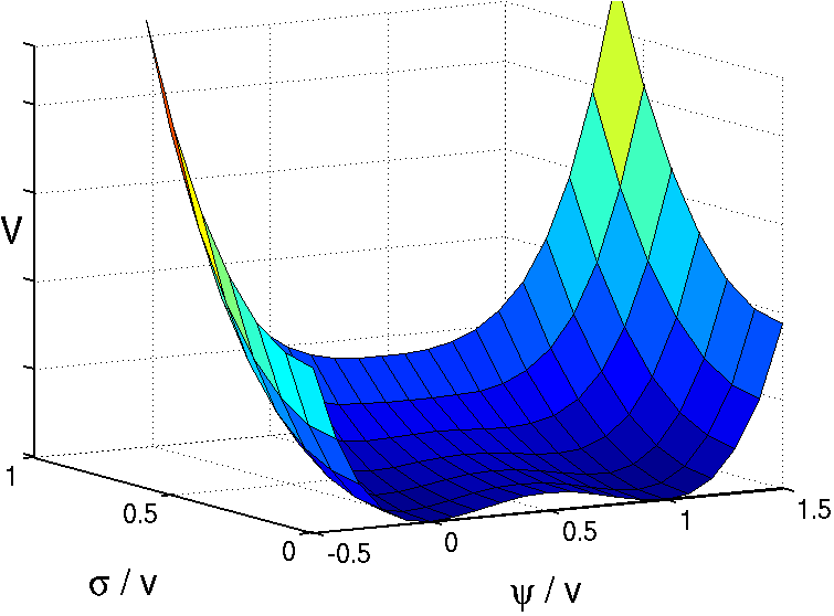
We assume canonical kinetic terms, as in the original renormalizable, globally-supersym- metric Wess-Zumino model, in which case the effective field-space metric is flat, i.e., the Kähler potential is minimal. Therefore the background equations are

$$H^{2} = \frac{1}{3M_{\rm pl}^{2}}\left(\frac{\dot{\varphi}_{a}\dot{\varphi}_{a}}{2}+V\right)\,,$$ (3.4)

$$\ddot{\varphi}_{a} = -3H\dot{\varphi}_{a}-V_{,a}\,,$$ (3.5)

and the perturbation equations are of the form given in (2.1), where we identify $\varphi_{a}=\{\psi,\sigma\}$.

3.1 Model Predictions for Cosmological Observables

In a generic two-field model, one may obtain any particular number of e-folds of inflation by choosing initial conditions on a one-dimensional contour in field space. In the present case we are interested in the Fourier modes of perturbations that cross the cosmological horizon roughly $50$ e-folds before inflation ends. Evolutions that pass through different locations along the $50$ e-fold contour can give rise to different observational predictions, and the values of the observational parameters that follow from different locations on this surface represent the exhaustive range of values the model can give yield for any particular choice of model parameters.

To determine whether the Wess-Zumino model can be compatible with current observational constraints for a particular choice of the model parameter $v$, therefore, we first perform a numerical search to find points close to the the contour that gives $50$ e-folds of inflation for some representative values of $v$. We allow points that lead to $N=50\pm 0.2$. We then use the tools described above to calculate the observables $n_{s}$, $r$ and $f_{\mathrm{NL}}$ that correspond to each position found. We aim to populate the contour sufficiently densely so that its shape is apparent, though the precise points found depend on the details of the search performed. We note that the value of $A$ does not affect the number of e-folds, $n_{s}$, $r$ or $f_{\mathrm{NL}}$. Hence, $A$ can be fixed independently at every position on the $50$ e-fold contour, so that the amplitude of $\zeta$ is in agreement with observations.

This analysis is performed in § 4.1. As we will see it is possible for the model to produce a range of signatures, and one might wonder whether all these possible signatures can actually be realized if, for example, inflation begins at some much higher energy scale so that many more than $50$ e-folds occur. In this case, although only the last $50$ e-folds play a role in the generation of observational signatures, the evolution during the preceding e-folds determines where on the $50$ e-fold contour the inflationary trajectory passes. In § 4.3, therefore, we look at the model in this alternative way, beginning the evolution on a constant-energy-density surface inside the eternal inflation boundary at large field values. Moreover, we follow Frazer [32], and ask not only what observational signatures can be realized from these initial conditions, but also what are the most likely signatures, by producing a probability distribution of the resulting values of $n_{s}$ and $r$ from an assumed uniform prior of the likelihood of initial conditions on the constant-energy-density surface.

Figure 2: Points on the $50$ e-fold contour are indicated with dark green stars for $v=40M_{\rm pl}$, with light green circles for $v=26M_{\rm pl}$, with blue squares for $v=10M_{\rm pl}$, and with black triangles for $v=5M_{\rm pl}$ (upper panel), and the corresponding values of the observables $n_{s}$ (middle left panel for $v=40M_{\rm pl}$ and $v=10M_{\rm pl}$, and lower left panel for $v=26M_{\rm pl}$ and $=5M_{\rm pl}$) and $r$ (middle right panel for $v=40M_{\rm pl}$ and $v=10M_{\rm pl}$, and lower left panel for $v=26M_{\rm pl}$ and $=5M_{\rm pl}$). The $n_{s}$ and $r$ plots are split between the middle and lower panels for visual clarity. In each case, the lines probed by the marked points are more extended the smaller the value of $v$. The field axes are chosen to be $(\hat{\psi}\equiv\psi/v,\hat{\sigma}\equiv\sigma/v)$.

4 Results

4.1 Predictions for $n_{s}$ and $r$

It was found in [4] that, if the initial condition was chosen so that $\sigma=0$, successful predictions for inflationary observables could be obtained for $v\sim 40M_{\rm pl}$ to $60M_{\rm pl}$. Accordingly, we first explore how the results of [4] can be generalized if one chooses $v=40M_{\rm pl}$ but allows initial conditions with $\sigma\neq 0$. Later we explore the possibilities if $\sigma\neq 0$ in the cases that $v=26M_{\rm pl}$, $v=10M_{\rm pl}$, and $v=5M_{\rm pl}$, values that were not consistent with the data if $\sigma=0$. The results for $v=40M_{\rm pl}$ and $v=26M_{\rm pl}$ can be compared with Table 1 of [4]

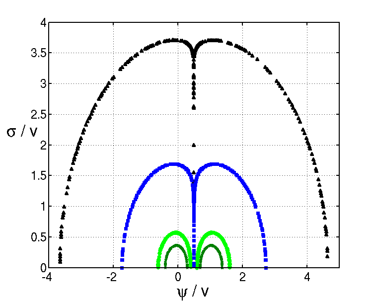
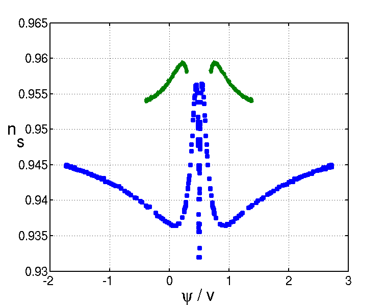
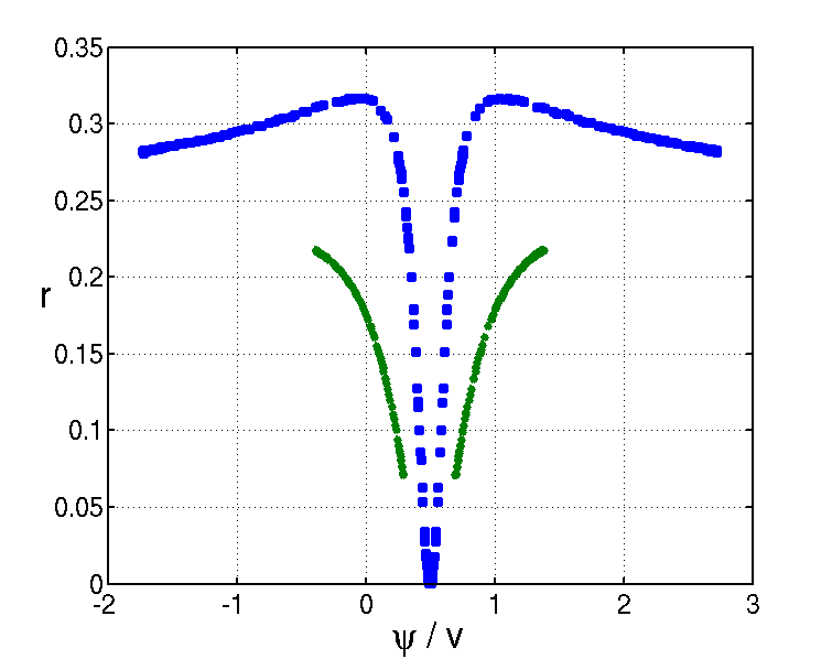
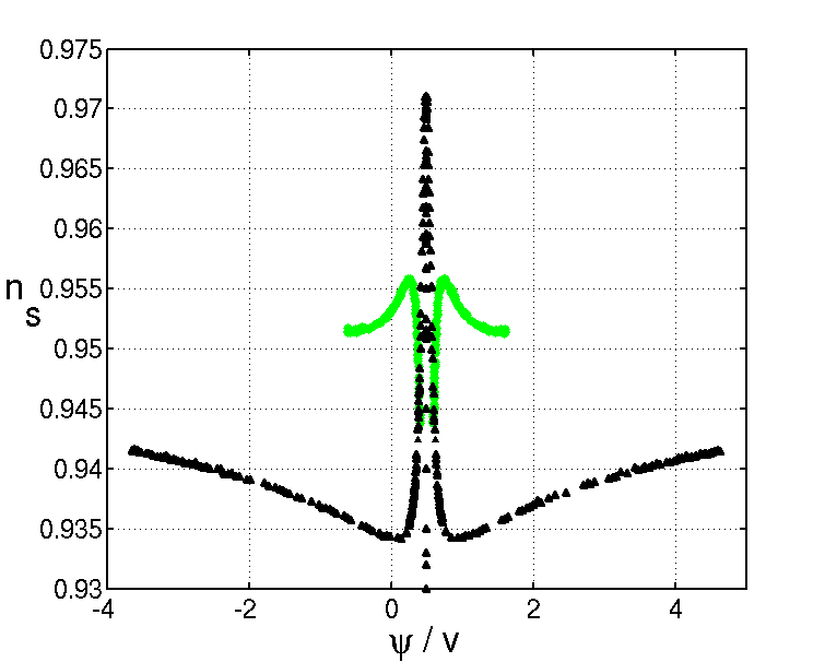
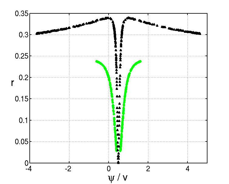
Positions on the $50$ e-fold contour for $v=40M_{\rm pl}$ are shown as the set of dark green star shaped points in the upper panel of Fig. 2, where the field axes are chosen to be $(\hat{\psi}\equiv\psi/v,\hat{\sigma}\equiv\sigma/v)$. The points run into one another in this case, but the contour can be identified as the inner most one on the figure. The contour takes the form of twin rings around the two minima of the potential, which intersect the real axis at $\psi\sim 12M_{\rm pl}$, $\hat{\psi}\sim 0.3$, (the solution found in [4]), at $\psi\sim-15.5M_{\rm pl}$, $\hat{\psi}\sim-0.39$, and at an equivalent pair of points that are their mirror images under reflection in the symmetry axis. The middle left panel of Fig. 2 shows the $n_{s}$ predictions for the points along the 50 e-fold contour for $v=40M_{\rm pl}$, and we see that all the points are consistent with the Planck constraint $n_{s}=0.9603\pm 0.0073$ at the 68% CL. However, we see in the middle right panel that the predictions for the tensor-to-scalar ratio, $r$, are in general less successful. Indeed, the only points along the left ring in the upper panel of Fig. 2 that yield $r<0.08$, and hence are consistent with the Planck data at the 68% CL, are those with $\psi>10M_{\rm pl}$. We see from the upper panel of Fig. 2 that these points also have $|\sigma|<10M_{\rm pl}$. These points and their mirror images along the right ring in the upper panel of Fig. 2 generalize the solution found in [4] for $v=40M_{\rm pl}$, which had $\sigma=0$. They represent trajectories evolving on the concave, hill, region of the potential, with most of the evolution in the $\psi$ direction.

Our generalized results for $v=40M_{\rm pl}$ and their compatibility with Planck constraints are summarized in Fig. 3 which is discussed further below.

Figure 3: The 50 e-fold results for $n_{s}$ and $r$ superimposed on the Planck constraints taken from Fig. 23 of Ref [1]. The $v=40M_{\rm pl}$ results are represented by the dark green stars (this is the smallest arc on the diagram), the $v=26M_{\rm pl}$ results by the light green circles, the $v=10M_{\rm pl}$ results by the blue squares, and the $v=5M_{\rm pl}$ results by the black triangles. Once again the lines probed by our results are more extended the smaller the value of $v$. For comparison, we also display the corresponding result for the Starobinsky model of $R^{2}$ inflation [5] with $50$ e-folds (red diamond).

Our second example is $v=10M_{\rm pl}$, marked on Fig. 2 by blue squares in the top and middle panels. In this case the restriction to the real axis discussed in [4] does not yield successful inflation in the hilltop region between the twin minima. For $\sigma=0$, one can obtain $50$ e-folds by choosing initial conditions extremely close to the top of the hill at $\psi=5M_{\rm pl}$, $\hat{\psi}\simeq 0.5$ (where N diverges to infinity), but for this case $n_{s}$ is much too small, in fact it is off the bottom of the plot in the middle left panel of Fig. 2. However, $50$ e-folds also results from positions along an arc extending from $(\psi,\sigma)\sim(5,0)$ through points with $\sigma\neq 0$ down to $(\psi,\sigma)\sim(-17,0)$ (or along the corresponding mirror contour). We see in the middle left panel that, for points corresponding to the left ring in the upper panel, suitable values of $n_{s}$ within the $n_{s}=0.9603\pm 0.0073$ range are found in the range $4.2M_{\rm pl}<\psi<4.8M_{\rm pl}$, $0.42<\psi<0.48$. In these cases, as seen in the middle right panel of Fig. 2, the corresponding values of $r$ are small, namely in the range $0.07>r>0.007$. The “good” inflationary trajectories start close to the minimum of the valley seen in Fig. 1 at $\psi=5M_{\rm pl}$ and large $\sigma$, roll along the $\sigma$ direction, and then fall off after the valley has turned into a ridge and roll to one of the two equivalent minima. We re-emphasize that the model seemed to be completely ruled out for $v=5M_{\rm pl}$, as long as one considered evolution only in the real direction, but that initial conditions consistent with observations can be found if one allows inflationary trajectories that start elsewhere in the two-field space.

These results and their compatibility with Planck constraints are summarized in Fig 3. We see that some initial conditions on the 50 e-fold contour for $v=10M_{\rm pl}$ (blue squares) yield values of $(n_{s},r)$ within the Planck 68% CL region, both for the joint distribution including tensors and the joint distribution including tensors and running. On the other hand, the line of $v=40M_{\rm pl}$ points (dark green stars) approaches but does not quite enter this region for the distribution including tensors alone for 50 e-folds.

In order to determine the how representative the values of $v$ we have considered thus far, finally we consider two further values, $v=26M_{\rm pl}$ and $v=5M_{\rm pl}$. The $v=26M_{\rm pl}$ results are represented by light green circles in the top and bottom panels of Fig. 2. For the hilltop $\sigma=0$ trajectory, although $r$ is small, $r\sim 0.03$, $n_{s}$ lies outside the $n_{s}=0.9603\pm 0.0073$ region. When other evolutions are considered, the $v=26M_{\rm pl}$ case exhibits behaviour intermediate between the $v=10M_{\rm pl}$ and $v=40M_{\rm pl}$ examples. Initial conditions with $-0.1M_{\rm pl}<\psi<9.1M_{\rm pl}$ provide values of $n_{s}$ in the range $n_{s}=0.9603\pm 0.0073$ but for this range we find $r>0.07$. From Fig. 3, one can see that no initial conditions lead to a value of $(n_{s},r)$ within the the Planck 68% CL region for the joint distribution without running, but points are found within the 68% CL region when tensors and running are included. The $v=5M_{\rm pl}$ case, represented in the top and bottom panels of Fig. 2 by black triangles, exhibits similar features to the $v=10M_{\rm pl}$ case, however, a broader range of $n_{s}$ and $r$ is possible, as is also seen in Fig. 3. As is seen from these figures, this case can be consistent with observations for similar valley/ridge trajectories to the ones described for the $v=10M_{\rm pl}$ example, despite being completely ruled out if only evolution in the real field direction were to be considered.

Some further comments are in order. First we note that for all the points shown in Fig. 3 we find that the running of the spectral index is within the range $-0.003<\alpha<0$. The magnitude of this negative running is smaller than that preferred by the Planck results at 68% CL level (see Fig. 23 of Ref. [1].), but well within the $2\sigma$ results which are consistent with zero running. Secondly, it is interesting to ask how the curves on Fig. 3 change if we select a different number of e-folds from the scales of interest crossing the horizon until the end of inflation. This true number is determined by the post inflationary dynamics such as the energy scale of reheating, and is generally taken to be between $40$ and $60$. Although we have not performed an exhaustive study, the rule of thumb is that the main change for curves on Fig. 3 is that they are shifted to the right and down with increasing number of e-folds, although the shapes are also slightly distorted. We choose $50$ as a representative number for the allowed range, and to allow comparison with Ref. [4]. Finally, we stress that in all the plots presented thus far, no inference should be drawn from the number of points populating different parts of the curve in Fig. 2 or Fig. 3, as this is a consequence of our scanning strategy.

Before closing this Section, we comment on the comparison of our two-field Wess-Zumino supersymmetric model for inflation with the Starobinsky model [5], whose excellent agreement with the Planck data (see Fig. 3) has recently prompted a plethora of interesting works finding Starobinsky-type potentials in supergravity models [34]. As we see in Fig. 3, the two-field Wess-Zumino model for $N=50$ e-foldings and $v=5M_{\rm pl}$ or $v=10M_{\rm pl}$ can yield results similar to the Starobinsky model, for particular initial conditions close to the $\sigma=0$ axis.

Figure 4: The 50 e-fold results for $n_{s}$, $r$ and $f_{\mathrm{NL}}$ (upper panel). And for clarity the plots for $f_{\mathrm{NL}}$ against $\psi/v$ and $f_{\mathrm{NL}}$ against $n_{s}$ (lower left and lower right panels respectively). As before $v=40M_{\rm pl}$ results are marked with dark green stars, $v=26M_{\rm pl}$ with light green circles, $v=10M_{\rm pl}$ with blue squares and $v=5M_{\rm pl}$ with black triangles.

4.2 Predictions for $f_{\mathrm{NL}}$

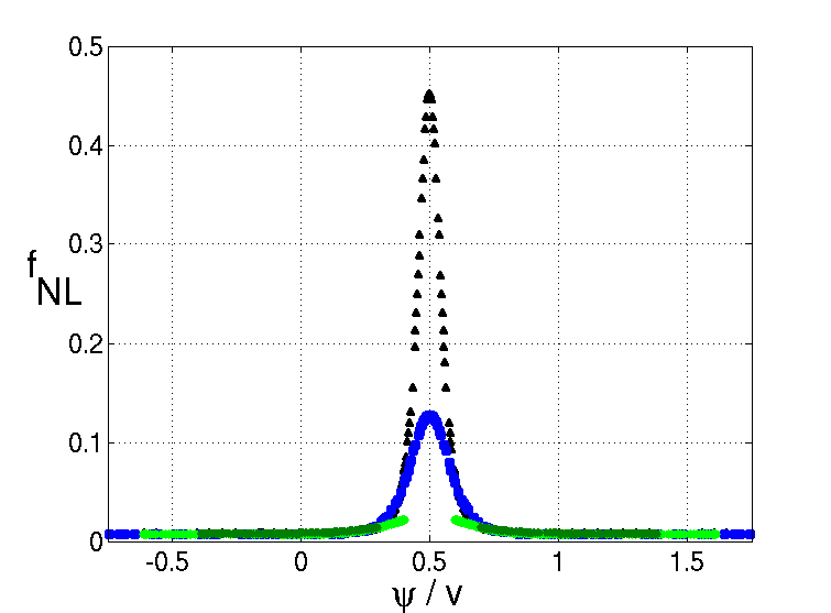
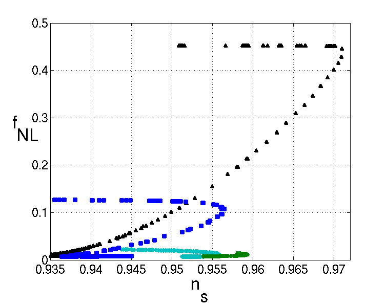
We now consider the Wess-Zumino model predictions for $f_{\mathrm{NL}}$. In simple models of inflation, a value of $f_{\mathrm{NL}}$ greater than the order of magnitude of the slow-roll parameters, i.e., $\gtrsim 1/N^{*}$ where $N^{*}$ is the observable number of e-folds, requires rather specific evolutions [35, 24, 36]. On the other hand, ridge-type evolutions such as those discussed above are known to play a rôle in producing larger values of $f_{\mathrm{NL}}$. We have explored the values of $f_{\mathrm{NL}}$ that are produced in the cases discussed above using the calculational method described earlier, with the results summarized in Fig 4.2. For the $v=40M_{\rm pl}$ and $v=26M_{\rm pl}$ cases, we can see that $f_{\mathrm{NL}}$ is never significantly enhanced above the slow-roll value. On the other hand, for $v=10M_{\rm pl}$ and $v=5M_{\rm pl}$, one can see that the “ridge” trajectories that leads to consistent $n_{s}$ and $r$ values do indeed lead to values of $f_{\mathrm{NL}}$ that are enhanced by over an order of magnitude, and that the largest enhancements we find are for the small values of $r$ that are favoured by the Planck measurements. For $v=10M_{\rm pl}$ we find that $f_{\mathrm{NL}}\lesssim 0.13$, and for $v=5M_{\rm pl}$ $f_{\mathrm{NL}}\lesssim 0.45$, too small to be probed by present experiments. These number are never-the-less an interesting signature of ridge trajectories, and are consistent with the “ridge” estimate of $f_{\mathrm{NL}}\sim-(5V_{,\sigma\sigma})/(6V)$ [37, 24, 38], despite this being derived for “separable potentials”, and not strictly being applicable to the current setting. For the Wess-Zumino model this estimate yields $f_{\mathrm{NL}}\sim 13.3/v^{2}$, and hence $f_{\mathrm{NL}}\sim 0.13$ for $v=10M_{\rm pl}$ and $f_{\mathrm{NL}}\sim 0.53$ for $v=5M_{\rm pl}$ in reasonable agreement with the results presented above.

Figure 5: Representative trajectories from a particular surface of constant energy density fixed outside of the the visible area. The blue solid lines are trajectories for the $v=40M_{\rm pl}$ case and the red dotted lines are for the $v=10M_{\rm pl}$ case. We see that while slow-roll is a good approximation these lines are almost identical when plotted on the rescaled $(\psi/v,\sigma/v)$ axis, but diverge as slow-roll ends. Inflation also ends in different positions for the two cases.

4.3 Statistical Predictions

Finally, we consider the probability distributions of possible inflationary predictions in the Wess-Zumino model assuming a uniform prior for initial conditions along a contour of constant potential energy density in a similar manner to Refs. [32, 39].

At much larger field values than are probed by the last $50$ e-folds of evolution for any inflationary trajectory, the Wess-Zumino potential has the approximate form $V\sim A(\psi^{2}+\sigma^{2})^{2}$. Thus, trajectories that start at large field values feel initially a potential that is approximately quartic in form, and the potential is rotationally symmetric. In this regime, constant-energy-density surfaces are therefore circles defined by $\psi^{2}+\sigma^{2}={\rm Const}$. By picking a particular value of the constant we choose a particular energy. In order to probe the model statistically, we parametrize this circle using polar coordinates, fix the initial energy and hence the initial radial coordinate, and pick initial angular coordinate values by drawing from a uniform distribution. This prior expresses maximal ignorance about the origin of trajectories.

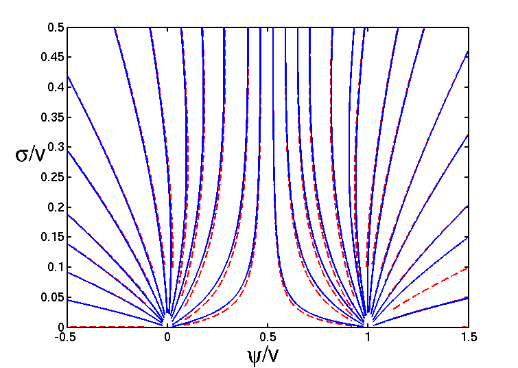
The trajectories that arise from such a surface can be seen in Fig. 5. The trajectories are initially straight lines that intersect successive circular uniform density surfaces. Therefore, as long as the field values are sufficiently large for the potential to be rotationally symmetric and a uniform prior is employed, the results we present are independent of the energy of the surface on which we choose to fix initial conditions. This would of course not be true if an alternative surface or prior were chosen, or the trajectories were initiated at a much lower energy scale. As the trajectories approach the region which contains the minima they begin to curve and eventually fall into one of the two minima as seen in Fig. 5.

The resultant distributions for $n_{s}$ and $r$ for the $v=40M_{\rm pl}$ and $v=10M_{\rm pl}$ cases are plotted in Fig. 6, respectively, where roughly $1000$ initial conditions are drawn from each of the prior distributions (the results are presented in histogram form, and so the vertical axis represents the number of points in each bin, rather than the normalised probability distribution). One can see in both cases that the bulk of the probability distribution corresponds to values of $r$ disfavoured by Planck. However, in the $v=40M_{\rm pl}$ case there is significant weight close to the preferred region.

It is an interesting question how to interpret these results. First we should note that we have effectively marginalised over the amplitude of the scalar power spectrum, since we have fixed this by implicitly normalising $A$. This is true also of previous statistical studies [32, 39], and in reality there is a distribution of amplitudes as well as of $n_{s}$ and $r$ given fixed model parameters. This makes it difficult to directly interpret the plotted distributions. Moreover, even if we were to take the distributions at face value, it is still an open question when to prefer one case over another. For example, comparing the $v=10M_{\rm pl}$ and $v=40M_{\rm pl}$ cases it is clear more of the probability in the $v=40M_{\rm pl}$ case is close to the observationally preferred values of $n_{s}$ and $r$. However, the $v=10M_{\rm pl}$ case has a small probability to get right in the middle of the preferred $(n_{s},r)$ region. We might consider therefore not weighting all initial conditions equally, but preferring those that get closer to the the preferred observational values of $n_{s}$ and $r$, and thus deriving some ultimate measure of the goodness of the model. Though that is beyond the scope of the present work. On the other hand, if we simply required the majority of the probability as plotted to be within the preferred $(n_{s},r)$ region, it is clear that neither value of $v$ could be considered consistent with observations.

Figure 6: The statistical distributions of $n_{s}$ and $r$ for the $v=40M_{\rm pl}$ (upper panel) and $v=10M_{\rm pl}$ (lower panel) cases. The results presented are not normalised, and so are histograms with the vertical axis referring to the number of points in each bin.

Before concluding this Section, we re-emphasize the point that, in this model, trajectories that begin their evolution in the quartic regime of the potential may plausibly find their way into the concave region for the requisite number of e-folds, as exemplified by the $v=40$ case discussed above – where a minority but significant amount of the probability distribution corresponds to evolutions on the concave region. This observation is interesting in light of recent criticisms of inflation [40]. Analyzing a single-field model of the form of (3.2) with $\theta=0$, it was argued in [40] that hilltop-like regimes preferred by Planck data Planck-compatible hilltop-like inflation would be exponentially unlikely. The reasoning was that they would require an energy density $\ll M_{P}^{4}$, whereas the primordial universe is likely to have had a much higher energy density, e.g., ${\cal O}(M_{P}^{4})$, in which case chaotic inflation with large field values and hence unacceptably large energy density would be exponentially more likely. However, the Wess-Zumino case studied here, which allows $\theta\neq 0$ in (3.2), is a counter-example showing that a realistic two-field dynamical model may allow as generic possibilities trajectories that find their way into a region preferred by cosmological observations, even if they originate at extremely high energy densities .

Finally we note that in considering the trajectories prior to the last $50$ e-folds, we have only considered the classical trajectory and not stochastic fluctuations about that path. While those fluctuations will be sub-dominant in each Hubble time outside of the eternal inflationary regime, the will accumulate over time and might still affect the statistics we have presented, and their effect on the statistics is an open question.

5 Conclusions

We have found in this exploration of the simplest Wess-Zumino model of inflation with real and imaginary field components several features of interest, that may also be present for more elaborate multi-field models. The introduction of the second (imaginary) degree of freedom opens up new possibilities for successful inflation that were not discussed in [4]. For example, we found that inflation is possible for values of the field scale $v$ that are much smaller than in the case where only the real part of the Wess-Zumino field is considered. We also found that much smaller values of $r$ could be obtained than in the previous simplified single-field “hill-top” treatment of this model. We also showed that $f_{\mathrm{NL}}$ could be much larger than usually found in slow-roll models, although the largest values we found were still too small to be observable in current experiments.

We also made an estimate of the statistical probability distribution of possible inflationary parameters, assuming pre-inflationary initial conditions corresponding to a uniform prior on a contour of constant energy density in the model parameter space. Although the probability distribution is not maximized in the regions of parameter space favoured by the Planck data, neither do these regions correspond to severe fine-tuning at least for the $v=40M_{\rm pl}$ case. The fact that one can find suitable inflationary trajectories starting from a high pre-inflationary energy density weakens one of the criticisms of single-field inflation made recently in [40], where it was argued that hill-top scenarios were unlikely to be realized.

We regard as very promising this exploration of the new inflationary possibilities that open up in two-field models. Although the Wess-Zumino model has an excellent theoretical pedigree, there are many proposals for more elaborate multi-field models that embody more attractive features. Staying within the supersymmetric framework, for example, it is desirable to incorporate the modifications to the effective potential induced by supergravity, and interesting to consider models in which local supersymmetry is broken dynamically [42]. The analysis of this paper indicates that these models might exhibit interesting novel features when their full complexity is considered.

Appendix A

In this appendix, in order that readers can reproduce our results, we summarise the super-horizon equations of motion for the scalar field fluctuations at second order, needed for Eq. (2.8) which we use to calculate $f_{\mathrm{NL}}$, and we also provide the relations we use to connect the field fluctuations to $\zeta$. The methods by which these are calculated are discussed extensively elsewhere [43]

We can write the second order equations of motion for the scalar field fluctuations, at second order in perturbation theory, as a set of first order equations of the compact form

$$\frac{{\rm d}x_{\alpha}}{{\rm d}N}=u_{\alpha\beta}x_{\beta}+\frac{1}{2}u_{\alpha\beta\gamma}x_{\beta}x_{\gamma}$$ (5.1)

where for convenience we use $N$ as the time variable, the Greek indices run over all fields and field momenta perturbations, and where $x_{\alpha}$ represents $(\delta\phi_{a},\delta\phi^{\prime}_{b})$. The $u$ matrices are

$$u_{ab} = 0\,,$$

$$u_{a\bar{b}} = \delta_{ab}\,,$$

$$u_{\bar{a}b} = -M^{2}_{ab}/H^{2}\,,$$

$$u_{\bar{a}\bar{b}} = (\epsilon-3)\delta_{ab}\,,$$

$$u_{abc} = 0\,,$$

$$u_{a\bar{b}c} = 0\,,$$

$$u_{a\bar{b}\bar{c}} = 0\,,$$

$$u_{\bar{a}bc} = -\frac{V_{,abc}}{H^{2}}+\left[\frac{V_{,ab}V_{,c}}{H^{4}M_{\rm pl}^{2}(3-\epsilon)}+(b\rightarrow c)\right]+\frac{V_{,bc}V_{,a}}{H^{4}M_{\rm pl}^{2}(3-\epsilon)}-\frac{2V_{,a}V_{,b}V_{,c}}{H^{6}M_{\rm pl}^{4}(3-\epsilon)^{2}}\,,$$

$$u_{\bar{a}\bar{b}c} = -\frac{V_{,a}V_{,c}\varphi^{\prime}_{b}}{H^{4}M_{\rm pl}^{4}(3-\epsilon)^{2}}+\frac{V_{,ac}\varphi^{\prime}_{b}}{H^{2}M_{\rm pl}^{2}(3-\epsilon)}\,,$$

$$u_{\bar{a}\bar{b}\bar{c}} = \frac{\varphi^{\prime}_{a}}{M_{\rm pl}^{2}}\delta_{bc}+\left[\frac{\varphi^{\prime}_{c}}{M_{\rm pl}^{2}}\delta_{ab}+(b\rightarrow c)\right]-\frac{V_{,a}\varphi^{\prime}_{b}\varphi^{\prime}_{c}}{H^{2}M_{\rm pl}^{4}(3-\epsilon)^{2}}+\frac{V_{,a}\delta_{bc}}{H^{2}M_{\rm pl}^{2}(3-\epsilon)}\,,$$ (5.2)

where the bar indicates field momentum indices (indices to be contracted with $\delta\varphi_{a}^{\prime}$) and no bar represents field indices, a dash indicates differentiation with respect to $N$, and $M^{2}_{ab}$ is defined below Eq. (2.1) (note that after the change in time variable is taken into account, comparing the first order $u$ matrices with Eq. (2.1), the only difference is the missing $k^{2}$ term which we neglect on super-horizon scales). These $u$ matrices are used in Eq. (2.8).

To convert to $\zeta$, Eqs. (2.9)-(2.10), we use the follow $N$ coeficients

$$N_{\alpha} = -\frac{1}{2\dot{H}}\frac{\partial H^{2}}{\partial X_{\alpha}}\,,$$

$$N_{\alpha\beta} = -\frac{1}{2\dot{H}}\frac{\partial^{2}H^{2}}{\partial X_{\alpha}X_{\beta}}-\frac{\partial}{\partial X_{(\alpha}}\left(\frac{1}{\dot{H}}\right)\frac{\partial H^{2}}{\partial X_{\beta)}}+\frac{1}{2\dot{H}}\frac{\partial}{\partial X_{\gamma}}\left(\frac{1}{2\dot{H}}\right)\frac{{\rm d}X_{\gamma}}{{\rm d}N}\frac{\partial H^{2}}{\partial X_{\alpha}}\frac{\partial H^{2}}{X_{\beta}}\,,$$ (5.3)

where $X_{\alpha}$ represents $(\varphi_{a},\varphi^{\prime}_{a})$ and where

$$\frac{\partial H^{2}}{\partial\varphi_{a}} = \frac{V_{,a}}{M_{\rm pl}^{2}(3-\epsilon)}\,,$$

$$\frac{\partial H^{2}}{\partial\varphi^{\prime}_{a}} = \frac{H^{2}\varphi^{\prime}_{a}}{M_{\rm pl}^{2}(3-\epsilon)}\,,$$

$$\frac{\partial^{2}H^{2}}{\partial\varphi_{a}\partial\varphi_{b}} = \frac{V_{,ab}}{M_{\rm pl}^{2}(3-\epsilon)}\,,$$

$$\frac{\partial^{2}H^{2}}{\partial\varphi_{a}\partial\varphi^{\prime}_{b}} = \frac{V_{,a}\varphi^{\prime}_{b}}{M_{\rm pl}^{4}(3-\epsilon)^{2}}\,,$$

$$\frac{\partial^{2}H^{2}}{\partial\varphi^{\prime}_{a}\partial\varphi^{\prime}_{b}} = \frac{2H^{2}\varphi^{\prime}_{a}\varphi^{\prime}_{b}}{M_{\rm pl}^{4}(3-\epsilon)^{2}}+\frac{H^{2}}{M_{\rm pl}^{2}(3-\epsilon)}\delta_{ab}\,,$$

$$\frac{\partial}{\partial\varphi_{a}}\left(\frac{1}{\dot{H}}\right) = \frac{-1}{\dot{H}H^{2}}\frac{\partial H^{2}}{\partial\varphi_{a}}\,,$$

$$\frac{\partial}{\partial\varphi^{\prime}_{a}}\left(\frac{1}{\dot{H}}\right) = \frac{H^{2}\varphi^{\prime}_{a}}{M_{\rm pl}^{2}{\dot{H}}^{2}}-\frac{1}{\dot{H}H^{2}}\frac{\partial H^{2}}{\partial\varphi^{\prime}_{a}}\,.$$ (5.4)