On Fence Patrolling by Mobile Agents

Abstract

Suppose that a fence needs to be protected (perpetually) by $k$ mobile agents with maximum speeds $v_{1},\ldots,v_{k}$ so that no point on the fence is left unattended for more than a given amount of time. The problem is to determine if this requirement can be met, and if so, to design a suitable patrolling schedule for the agents. Alternatively, one would like to find a schedule that minimizes the idle time, that is, the longest time interval during which some point is not visited by any agent. We revisit this problem, introduced by Czyzowicz et al. (2011), and discuss several strategies for the cases where the fence is an open and a closed curve, respectively.

In particular: (i) we disprove a conjecture by Czyzowicz et al. regarding the optimality of their Algorithm $\mathcal{A}_{2}$ for unidirectional patrolling of a closed fence; (ii) we present an algorithm with a lower idle time for patrolling an open fence, improving an earlier result of Kawamura and Kobayashi.

Keywords: mobile agents, fence patrolling, idle time, approximation algorithm.

1 Introduction

A set of $k$ mobile agents with (possibly distinct) maximum speeds $v_{i}$ ($i=1,\ldots,k$) are in charge of guarding or in other words patrolling a given region of interest. Patrolling problems find applications in the field of robotics where surveillance of a region is necessary. An interesting one-dimensional variant have been introduced by Czyzowicz et al. [7], where the agents move along a rectifiable Jordan curve representing a fence. The fence is either a closed curve (the boundary of a compact region in the plane), or an open curve (the boundary between two regions). For simplicity (and without loss of generality) it can be assumed that the open curve is a line segment and the closed curve is a circle. The movement of the agents over the time interval $[0,\infty)$ is described by a patrolling schedule, where the speed of the $i$th agent, $a_{i}$ ($i=1,\ldots,k$), may vary between zero and its maximum value $v_{i}$ in any of the two moving directions (left or right).

Given a closed or open fence of length $\ell$ and maximum speeds $v_{1},\ldots,v_{k}>0$ of $k$ agents, the goal is to find a patrolling schedule that minimizes the idle time $I$, defined as the longest time interval in $[0,\infty)$ during which a point on the fence remains unvisited, taken over all points. A straightforward volume argument [7] yields the lower bound $I\geq\ell/\sum_{i=1}^{k}v_{i}$ for an (open or closed) fence of length $\ell$. A patrolling algorithm computes a patrolling schedule for a given fence and set of speeds $v_{1},\ldots,v_{k}>0$.

For an open fence (line segment), Czyzowicz et al. [7] proposed a simple partitioning strategy, algorithm $\mathcal{A}_{1}$, where each agent moves back and forth perpetually in a segment whose length is proportional with its speed. Specifically, for a segment of length $\ell$ and $k$ agents with maximum speeds $v_{1},\ldots,v_{k}$, algorithm $\mathcal{A}_{1}$ partitions the segment into $k$ pieces of lengths $\ell v_{i}/\sum_{j=1}^{k}v_{j}$, and schedules the $i$th agent to patrol the $i$th interval with speed $v_{i}$. Algorithm $\mathcal{A}_{1}$ has been proved to be optimal for uniform speeds [7], i.e., when all maximum speeds are equal. Algorithm $\mathcal{A}_{1}$ achieves an idle time $2\ell/\sum_{i=1}^{k}v_{i}$ on a segment of length $\ell$, and so $\mathcal{A}_{1}$ is a 2-approximation algorithm for the shortest idle time. It has been conjectured [7, Conjecture 1] that $\mathcal{A}_{1}$ is optimal for arbitrary speeds, however this was disproved by Kawamura and Kobayashi [9]: they selected speeds $v_{1},\ldots,v_{6}$ and constructed a schedule for $6$ agents that achieves an idle time of $\frac{41}{42}\,\left(2\ell/\sum_{i=1}^{k}v_{i}\right)$.

A patrolling algorithm $\mathcal{A}$ is universal if it can be executed with any number of agents $k$ and any speed setting $v_{1},\ldots,v_{k}>0$ for the agents. For example, $\mathcal{A}_{1}$ above is universal, however certain algorithms (e.g., algorithm $\mathcal{A}_{3}$ in Section 3 or the algorithm in Section 4) can only be executed with certain speed settings or number of agents, i.e., they are not universal.

For the closed fence (circle), no universal algorithm has been proposed to be optimal. For uniform speeds (i.e., $v_{1}=\ldots=v_{k}=v$), it is not difficult to see that placing the agents uniformly around the circle and letting them move in the same direction yields the shortest idle time. Indeed, the idle time in this case is $\ell/(kv)=\ell/\sum_{i=1}^{k}v_{i}$, matching the lower bound mentioned earlier.

For the variant in which all agents are required to move in the same direction along a circle of unit length (say clockwise), Czyzowicz et al. [7, Conjecture 2] conjectured that the following algorithm $\mathcal{A}_{2}$ always yields an optimal schedule. Label the agents so that $v_{1}\geq v_{2}\geq\ldots\geq v_{k}>0$. Let $r$, $1\leq r\leq k$, be an index such that $\max_{1\leq i\leq k}iv_{i}=rv_{r}$. Place the agents at equal distances of $1/r$ around the circle, so that each moves clockwise at the same speed $v_{r}$. Discard the remaining agents, if any. Since all agents move in the same direction, we also refer to $\mathcal{A}_{2}$ as the “runners” algorithm. It achieves an idle time of $1/\max_{1\leq i\leq k}iv_{i}$ [7, Theorem 2]. Observe that $\mathcal{A}_{2}$ is also universal.

Historical perspective.

Multi-agent patrolling is a variation of the fundamental problem of multi-robot coverage [4, 5], studied extensively in the robotics community. A variety of models has been considered for patrolling, including deterministic and randomized, as well as centralized and distributed strategies, under various objectives [1, 8]. Idleness, as a measure of efficiency for a patrolling strategy, was introduced by Machado et al. [10] in a graph setting; see also the article by Chevaleyre [4].

The closed fence patrolling problem is reminiscent of the classical lonely runners conjecture, introduced by Wills [11] and Cusick [6], independently, in number theory and discrete geometry. Assume that $k$ agents run clockwise along a circle of length $1$, starting from the same point at time $t=0$. They have distinct but constant speeds (the speeds cannot vary, unlike in the model considered in this paper). A runner is called lonely when he/she is at distance of at least $\frac{1}{k}$ from any other runner (along the circle). The conjecture asserts that each runner $a_{i}$ is lonely at some time $t_{i}\in(0,\infty)$. The conjecture has only been confirmed for up to $k=7$ runners [2, 3].

Notation and terminology.

A unit circle is a circle of unit length. We parameterize a line segment and a circle of length $\ell$ by the interval $[0,\ell]$. A schedule of $k$ agents consists of $k$ functions $f_{i}:[0,\infty]\rightarrow[0,\ell]$, for $i=1,\ldots,k$, where $f_{i}(t)$ is the position of agent $i$ at time $t$. Each function $f_{i}$ is continuous (for a closed fence, the endpoints of the interval $[0,\ell]$ are identified), it is piecewise differentiable, and its derivative (speed) is bounded by $|f_{i}^{\prime}|\leq v_{i}$. A schedule is called periodic with period $t_{0}>0$ if $f_{i}(t)=f_{i}(t+t_{0})$ for all $i=1,\ldots,k$ and $t\geq 0$. The idle time $I$ of a schedule is the length of the maximum (open) time interval $(t_{1},t_{2})$ such that there is a point $x\in[0,\ell]$ where $f_{i}(t)\neq x$ for all $i=1,\ldots,k$ and $t\in(t_{1},t_{2})$. For a given fence (closed or open) of length $\ell$ and given maximum speeds $v_{1},\ldots,v_{k}$, ${\tt idle}(\mathcal{A})$ denotes the idle time of a schedule produced by algorithm $\mathcal{A}$.

We use position-time diagrams to plot the agent trajectories with respect to time. One axis represents the position $f_{i}(t)$ of the agents along the fence and the other axis represents time. In Fig. 1, for instance, the horizontal axis represents the position of the agents along the fence and the vertical axis represents time. In Fig. 2, however, the vertical axis represents the position and the vertical axis represents time. A schedule with idle time $I$ is equivalent to a covering problem in such a diagram (see Fig. 1). For a straight-line (i.e., constant speed) trajectory between points $(x_{1},y_{1})$ and $(x_{2},y_{2})$ in the diagram, construct a shaded parallelogram with vertices, $(x_{1},y_{1})$, $(x_{1},y_{1}+I)$, $(x_{2},y_{2})$, $(x_{2},y_{2}+I)$, where $I$ denotes the desired idle time and the shaded region represents the covered region. In particular, if an agent stays put in a time-interval, the parallelogram degenerates to a vertical segment. A schedule for the agents ensures idle time $I$ if and only if the entire area of the diagram in the time interval $[I,\infty)$ is covered.

To evaluate the efficiency of a patrolling algorithm $\mathcal{A}$, we use the ratio $\rho={\tt idle}(\mathcal{A})/{\tt idle}(\mathcal{A}_{1})$ between the idle times of $\mathcal{A}$ and the partition-based algorithm $\mathcal{A}_{1}$. Lower values of $\rho$ indicate better (more efficient) algorithms. Recall however that certain algorithms can only be executed with certain speed settings or number of agents.

We write $H_{n}=\sum_{i=1}^{n}1/i$ for the $n$th harmonic number.

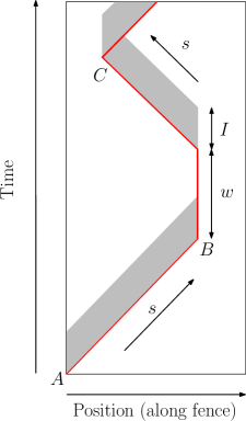
Figure 1: Agent moving with speed $s$ from $A$ to $B$, waiting at $B$ for time $w$ and then moving from $B$ to $C$ with speed $s$.

Our results.

1. Consider the unidirectional unit circle (where all agents are required to move in the same direction).

   (i) We disprove a conjecture by Czyzowicz et al. [7, Conjecture 2] regarding the optimality of Algorithm $\mathcal{A}_{2}$. Specifically, we construct a schedule for $32$ agents with harmonic speeds $v_{i}=1/i$, $i=1,\ldots,32$, that has an idle time strictly less than $1$. In contrast, Algorithm $\mathcal{A}_{2}$ yields a unit idle time for harmonic speeds (${\tt idle}(\mathcal{A}_{2})=1$), hence it is suboptimal. See Theorem 1, Section 2.

   (ii) For every $\tau\in(0,1]$ and $t\geq\tau$, there exists a positive integer $k=k(t)\leq e^{4t/\tau^{2}}$ and a schedule for the system of $k$ agents with harmonic speeds $v_{i}=1/i$, $i=1,\ldots,k$, that ensures an idle time at most $\tau$ during the time interval $[0,t]$. See Theorem 2, Section 2.

2. Consider the open fence patrolling. For every integer $x\geq 2$, there exist $k=4x+1$ agents with $\sum_{i=1}^{k}v_{i}=16x+1$ and a guarding schedule for a segment of length $25x/3$. Alternatively, for every integer $x\geq 2$ there exist $k=4x+1$ agents with suitable speeds $v_{1},\ldots,v_{k}$, and a guarding schedule for a unit segment that achieves idle time at most $\frac{48x+3}{50x}\,\frac{2}{\sum_{i=1}^{k}v_{i}}$. In particular, for every $\varepsilon>0$, there exist $k$ agents with suitable speeds $v_{1},\ldots,v_{k}$, and a guarding schedule for a unit segment that achieves idle time at most $\left(\frac{24}{25}+\varepsilon\right)\,\frac{2}{\sum_{i=1}^{k}v_{i}}$. This improves the previous bound of $\frac{41}{42}\,\frac{2}{\sum_{i=1}^{k}v_{i}}$ by Kawamura and Kobayashi [9]. See Theorem 3, Section 4.

3. Consider the bidirectional unit circle.

   (i) For every $k\geq 4$, there exist maximum speeds $v_{1}\geq v_{2}\geq\ldots\geq v_{k}$ and a new patrolling algorithm $\mathcal{A}_{3}$ that yields an idle time better than that achieved by both $\mathcal{A}_{1}$ and $\mathcal{A}_{2}$. In particular, for large $k$, the idle time of $\mathcal{A}_{3}$ with these speeds is about $2/3$ of that achieved by $\mathcal{A}_{1}$ and $\mathcal{A}_{2}$. See Proposition 1, Section 3.

   (ii) For every $k\geq 2$, there exist maximum speeds $v_{1}\geq v_{2}\geq\ldots\geq v_{k}$ so that there exists an optimal schedule (patrolling algorithm) for the circle that does not use up to $k-1$ of the agents $a_{2},\ldots,a_{k}$. In contrast, for a segment, any optimal schedule must use all agents. See Proposition 2, Section 3.

   (iii) There exist settings in which if all $k$ agents are used by a patrolling algorithm, then some agent(s) need overtake (pass) other agent(s). This partially answers a question left open by Czyzowicz et al. [7, Section 3]. See the remark at the end of Section 3.

2 Unidirectional Circle Patrolling

A counterexample for the optimality of algorithm $\mathcal{A}_{2}$.

We show that Algorithm $\mathcal{A}_{2}$ by Czyzowicz et al. [7] for unidirectional circle patrolling is not always optimal. We consider agents with harmonic speeds $v_{i}=1/i$, $i\in\mathbb{N}$. Obviously, for this setting we have ${\tt idle}(\mathcal{A}_{2})=1$, which is already achieved by the agent $a_{1}$ with the highest (here unit) speed. We design a periodic schedule (patrolling algorithm) for $k=32$ agents with idle time $I<1$. In this schedule, agent $a_{1}$ moves continuously with unit speed, and it remains to schedule agents $a_{2},\ldots,a_{32}$ such that every point is visited at least one more time in the unit length open time interval between two consecutive visits of $a_{1}$. We start with a weaker claim, for closed intervals but using only $6$ agents.

Lemma 1.

Consider the unit circle, where all agents are required to move in the same direction. For k=6 agents of harmonic speeds $v_{i}=1/i$, $i=1,\ldots,6$, there is a schedule where agent $a_{1}$ moves continuously with speed $1$, and every point on the circle is visited by some other agent in every closed unit length time interval between two consecutive visits of $a_{1}$.

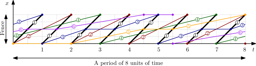
Figure 2: A periodic schedule of $6$ agents of speeds $1/i$, $i=1,\ldots,6$, on a unit circle with period $8$. Agent $a_{1}$ moves continuously with speed $1$. Each point is visited by one of the agents $a_{2},a_{3},a_{4},a_{5},a_{6}$ between any two consecutive visits of agent $a_{1}$.

Proof.

Our proof is constructive. We construct a periodic schedule for the $6$ agents with period $8$; refer to Fig. 2. Agents $a_{1}$, $a_{2}$ and $a_{4}$ continuously move with maximum speed, while agents $a_{3}$, $a_{5}$ and $a_{6}$ each stop at certain times in their movements. Their schedule in one period $t\in[0,8]$ is given by the following piecewise linear functions.

$$f_{1}(t)=t\mod 1,\hskip 28.45274ptf_{2}(t)=t/2\mod 1,\hskip 28.45274ptf_{4}(t)=(t-3)/4\mod 1.$$

$$f_{3}(t)=\left\{\begin{array}[]{ll}(t-1)/3\mod 1&\mbox{\rm for }t\in[0,2.5]\cup[7.5,8]\\ 0.5&\mbox{\rm for }t\in[2.5,3.5]\cup[6.5,7.5]\\ (t-2)/3\mod 1&\mbox{\rm for }t\in[3.5,6.5]\\ t/3\mod 1&\mbox{\rm for }t\in[7.5,8].\end{array}\right.$$

$$f_{5}(t)=\left\{\begin{array}[]{ll}0&\mbox{\rm for }t\in[0,2]\\ (t-2)/5\mod 1&\mbox{\rm for }t\in[2,4.5]\\ 0.5&\mbox{\rm for }t\in[4.5,5.5]\\ (t-3)/5\mod 1&\mbox{\rm for }t\in[5.5,8].\end{array}\right.$$

$$f_{6}(t)=\left\{\begin{array}[]{ll}(t-3.5)/6\mod 1&\mbox{\rm for }t\in[0,0.5]\\ 0.5&\mbox{\rm for }t\in[0.5,1.5]\\ (t-4.5)/6\mod 1&\mbox{\rm for }t\in[1.5,4.5]\\ 1&\mbox{\rm for }t\in[4.5,5.5]\\ (t-5.5)/6\mod 1&\mbox{\rm for }t\in[5.5,8].\end{array}\right.$$

∎

Theorem 1.

Consider the unit circle, where all agents are required to move in the same direction. For $32$ agents of harmonic speeds $v_{i}=1/i$, $i=1,\ldots,32$, there is a periodic schedule with idle time strictly less than $1$.

Proof.

Agents $a_{1},\ldots,a_{6}$ follow the periodic schedule described in Lemma 1. A time-position pair $(t,x)\in[0,8)\times[0,1)$ is a critical point in the time-position diagram if point $x$ on the fence is not traversed by any agent in the open time interval $(t,t+1)$. There are exactly $12$ critical points in the schedule in Fig. 2. Specifically, these points are $(j,0)$ for $j=0,1,\ldots,7$; and $(j+\frac{1}{2},\frac{1}{2})$ for $j=1,3,5,7$.

For each critical point $(t,x)$, we assign one, two, or four agents such that they jointly traverse a small neighborhood of the critical point in each period in the periodic schedule.

We schedule agents $a_{7}$ and $a_{8}$ to move continuously with speed $1/8$, as follows.

$$f_{7}(t)=\frac{1}{8}\left(t-\frac{1}{3}\right)\mod 1,\hskip 28.45274ptf_{8}(t)=\frac{1}{8}\left(t-\frac{7}{3}\right)\mod 1.$$

Agent $a_{7}$ traverses the unit intervals of the critical points $(0,0)$ and $(3+\frac{1}{2},\frac{1}{2})$; and agent $a_{8}$ traverses the unit intervals of the critical points $(2,0)$ and $(5+\frac{1}{2},\frac{1}{2})$. We are left with $8$ critical points, which will be taken care of by agents $a_{9},\ldots,a_{32}$.

Agents $a_{9},\ldots,a_{16}$ are scheduled to move with constant speed $1/16$. These $8$ agents form $4$ pairs, where each pair is responsible to visit the neighborhood of a critical point in each period of length $8$ (each agent in a pair returns to the same critical point after $16$ units of time). Finally, agents $a_{17},\ldots,a_{32}$ move with constant speed $1/32$. These $16$ agents form 4 quadruples, where each quadruple is responsible to visit the neighborhood of a critical point in each period of $8$ (each agent in a quadruple returns after $32$ units of time).

This schedule ensures that every point on the fence within a small neighborhood of the $12$ critical points is visited by some agent within every time interval of length $1-\varepsilon$, where $\varepsilon>0$ is a sufficiently small constant. Apart from these neighborhoods, the first $6$ agents already visit every point within every time interval of length $1-\varepsilon$ if $\varepsilon>0$ is sufficiently small. ∎

Remark.

In Theorem 1, we required that all agents move in the same direction (clockwise) along the unit circle, but we allowed agents to stop (i.e., have zero speed). If all agents are required to maintain a strictly positive speed, the proof of Theorem 1 would still go through: in this case, agents $a_{3}$, $a_{5}$ and $a_{6}$ could move at an extremely slow but positive speed instead of stopping. As a result, some points at the neighborhoods of the $12$ critical points would remain unvisited for 1 unit of time (this frequency is maintained by agent $a_{1}$ alone). However, agents $a_{7},\ldots,a_{32}$ would still ensure that every point in these neighborhoods is also visited within every time interval of length $1-\varepsilon$.

Finite time patrolling.

Interestingly enough, we can achieve any prescribed idle time below $1$ for an arbitrarily long time in this setting, provided we choose the number of agents $k$ large enough.

Theorem 2.

Consider the unit circle, where all agents are required to move in the same direction. For every $0<\tau\leq 1$ and $t\geq\tau$, there exists $k=k(t)\leq e^{4t/\tau^{2}}$ and a schedule for the system of $k$ agents with maximum speeds $v_{i}=1/i$, $i=1,\ldots,k$, that ensures an idle time $\leq\tau$ during the time interval $[0,t]$.

Proof.

We construct a schedule with an idle time at most $\tau$. Let agent $a_{1}$ start at time $0$ and move clockwise at maximum (unit) speed, i.e., $a_{1}(t)=t\mod 1$ denotes the position on the unit circle of agent $a_{1}$ at time $t$. Assume without loss of generality that $t$ is a multiple of $\tau$, i.e., $t=m\tau$, where $m$ is a natural number. Divide the time interval $[0,t]$ into $2m$ subintervals of length $\tau/2$. For $j=1,\ldots,2m$, $[(j-1)\tau/2,j\tau/2]$ is the $j$th interval.

For each $j$, cover the unit circle $C$ so that every point of $C$ is visited at least once by some agent. This ensures that each point of the circle is visited at least once in the time interval $[0,\tau/2]$ and no two consecutive visits to any one point are separated in time by more than $\tau$ thereafter until time $t$, as required.

To achieve the covering condition in each interval $j$, we use the first agent ($a_{1}$, of unit speed), and as many other unused agents as needed. The ‘origin’ on $C$ is reset to the current position of $a_{1}$ at time $(j-1)\tau/2$, i.e., the beginning of the current time interval. So the fastest agent is used (continuously) in all $2m$ time intervals. Agent $a_{1}$ can cover a distance of $\tau/2$ during one interval. From its endpoint, at time $(j-1)\tau/2$, start the unused agent with the smallest index, say $i_{1}(j)$; this agent can cover a distance of $\frac{\tau}{2}\frac{1}{i_{1}(j)}$ during the interval. Continue in the same way using new agents, all starting at time $(j-1)\tau/2$, until the entire circle $C$ is covered; let the index of the last agent used be $i_{2}(j)$. The covering condition can be written as:

$$\frac{\tau}{2}\left(1+\sum_{i=i_{1}(j)}^{i_{2}(j)}\frac{1}{i}\right)\geq 1,\textup{ or equivalently, }1+\sum_{i=i_{1}(j)}^{i_{2}(j)}\frac{1}{i}\geq\frac{2}{\tau}.$$ (1)

For example, if $\tau=2/3$: $j=1$ requires agents $a_{1}$ through $a_{11}$, since $H_{11}\geq 3$, but $H_{10}<3$; $j=2$ requires agents $a_{1}$ and agents $a_{12}$ through $a_{85}$, since $1+(H_{85}-H_{11})\geq 3$, but $1+(H_{84}-H_{11})<3$.

We now bound from above the total number $k$ of distinct agents used i.e., with speeds $1/i$, for $i=1,\ldots,k$. Observe that the covering condition (1) may lead to overshooting the target. Because the harmonic series has decreasing terms, the overshooting error cannot exceed the term $\frac{1}{i_{2}(1)+1}$ for $\tau=1$, namely $1/5$ (the overshooting for $\tau=1$ is only $\frac{1}{3}-\frac{1}{4}=\frac{1}{12}<\frac{1}{5}$). So inequality (1) becomes

$$\frac{2}{\tau}\leq 1+\sum_{i=i_{1}(j)}^{i_{2}(j)}\frac{1}{i}\leq\frac{2}{\tau}+\frac{1}{5}.$$ (2)

Recall that $t=m\tau$. By adding inequality (2) over all $2m$ time intervals yields (in equivalent forms)

$$H_{k}-1+\frac{8m}{5}\leq\frac{4m}{\tau},\textup{ or }H_{k}\leq\frac{4t}{\tau^{2}}+1-\frac{8t}{5\tau}.$$ (3)

For $t\geq\tau$ we have $1\leq\frac{8t}{5\tau}$. Since $\ln{k}\leq H_{k}$, it follows from (3) that

$$\ln{k}\leq\frac{4t}{\tau^{2}},\textup{ or }k\leq e^{4t/\tau^{2}},$$

as required. ∎

3 Bidirectional Circle Patrolling

A new schedule for closed fence patrolling.

Czyzowicz et al. [7, Theorem 5] showed that for $k=3$ there exist maximum speeds $v_{1},v_{2},v_{3}$ and a schedule that achieves a shorter idle time than both algorithm $\mathcal{A}_{1}$ and $\mathcal{A}_{2}$, namely $35/36$ versus $12/11$ and $1$. We extend this result for all $k\geq 4$.

We propose a new algorithm, $\mathcal{A}_{3}$ for maximum speeds $v_{1}\geq v_{2}\geq\ldots\geq v_{k}>0$, and then show that $\mathcal{A}_{3}$ outperforms both $\mathcal{A}_{1}$ and $\mathcal{A}_{2}$ for some speed settings for all $k\geq 4$.

We will need $v_{1}>v_{2}$ in this algorithm. Place the $k-1$ agents $a_{2},\ldots,a_{k}$ at equal distances, $x$ on the unit circle, and let them move all clockwise perpetually at the same speed $v_{k}$; we say that $a_{2},\ldots,a_{k}$ make a “train”. Let $a_{1}$ move back and forth (i.e., clockwise and counterclockwise) perpetually on the moving arc of length $1-(k-2)x$, i.e., between the start and the end of the train. Refer to Fig. 3.

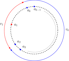
Figure 3: Train algorithm: the train $a_{2},\ldots,a_{k}$ moving unidirectionally with speed $v_{k}$ and the bidirectional agent $a_{1}$ with speed $v_{1}$.

Proposition 1.

For every $k\geq 4$, there exist maximum speeds $v_{1}>v_{2}\geq\ldots\geq v_{k}$ such that algorithm $\mathcal{A}_{3}$ achieves a shorter idle time than $\mathcal{A}_{1}$ and $\mathcal{A}_{2}$. In particular, for large $k$, the idle time achieved by the train algorithm is about $2/3$ of those achieved by $\mathcal{A}_{1}$ and $\mathcal{A}_{2}$.

Proof.

Consider the speed setting $v_{1}=a$, $v_{2}=\ldots=v_{k}=b$, where $a>b>0$, and $\max_{1\leq i\leq k}iv_{i}=kb$ (i.e., $a\leq kb$). Put $y=1-(k-2)x$. To determine the idle time, $x/b$, write:

$$[1-(k-2)x]\left(\frac{1}{a-b}+\frac{1}{a+b}\right)=\frac{x}{b},\textup{ or equivalently, }\frac{2ay}{a^{2}-b^{2}}=\frac{1-y}{(k-2)b}.$$

Solving for $x/b$ yields

$${\tt idle}(\mathcal{A}_{3})=\frac{2a}{a^{2}-b^{2}+2(k-2)ab}.$$

For our speed setting, we also have

$${\tt idle}(\mathcal{A}_{1})=\frac{2}{a+(k-1)b},\textup{ and }{\tt idle}(\mathcal{A}_{2})=\frac{1}{kb}.$$

Write $t=a/b$. It can be checked that for $k\geq 4$, ${\tt idle}(\mathcal{A}_{3})\leq{\tt idle}(\mathcal{A}_{1})$ and ${\tt idle}(\mathcal{A}_{3})\leq{\tt idle}(\mathcal{A}_{2})$ when $a^{2}-b^{2}-4ab\geq 0$, i.e., $t\geq 2+\sqrt{5}$. In particular, for $a=1$, and $b=1/k$ (note that $a\leq kb$), we have

$${\tt idle}(\mathcal{A}_{3})=\frac{2}{1-1/k^{2}+2(k-2)/k}\underset{k\to\infty}{\longrightarrow}\,\frac{2}{3},$$

while

$${\tt idle}(\mathcal{A}_{1})=\frac{2}{1+(k-1)/k}\underset{k\to\infty}{\longrightarrow}\,1,\textup{ and }{\tt idle}(\mathcal{A}_{2})=\frac{1}{k(1/k)}=1.$$ ∎

Useless agents for circle patrolling.

Czyzowicz et al. [7] showed that for $k=2$ there are maximum speeds for which an optimal schedule does not use one of the agents. Here we extend this result for all $k\geq 2$:

Proposition 2.

(i) For every $k\geq 2$, there exist maximum speeds $v_{1}\geq v_{2}\geq\ldots\geq v_{k}>0$ and an optimal schedule for the circle with these speeds that does not use up to $k-1$ of the agents $a_{2},\ldots,a_{k}$.

(ii) In contrast, for a segment, any optimal schedule must use all agents.

Proof.

(i) Let $v_{1}=1$ and $v_{2}=\ldots=v_{k}=\varepsilon/k$, for a small positive $\varepsilon\leq 1/300$, and $C$ be a unit circle. Obviously by using agent $a_{1}$ alone (moving perpetually clockwise) we can achieve unit idle time. Assume for contradiction that there exists a schedule achieving an idle time less than $1$. Let $a_{1}(t)=t\mod 1$ denote the position of agent $a_{1}$ at time $t$. Assume without loss of generality that $a_{1}(0)=0$ and consider the time interval $[0,2]$. For $2\leq i\leq k$, let $J_{i}$ be the interval of points visited by agent $a_{i}$ during the time interval $[0,2]$, and put $J=\cup_{i=2}^{k}J_{i}$. We have $|J_{i}|\leq 2\varepsilon/k$, thus $|J|\leq 2\varepsilon$. We make the following observations:

1. $a_{1}(1)\in[-2\varepsilon,2\varepsilon]$. Indeed, if $a_{1}(1)\notin[-2\varepsilon,2\varepsilon]$, then either some point in $[-2\varepsilon,2\varepsilon]$ is not visited by any agent during the time interval $[0,1]$, or some point in $C\setminus[-2\varepsilon,2\varepsilon]$ is not visited by any agent during the time interval $[0,1]$.

2. $a_{1}$ has done almost a complete (say, clockwise) rotation along $C$ during the time interval $[0,1]$, i.e., it starts at $0\in[-2\varepsilon,2\varepsilon]$ and ends in $[-2\varepsilon,2\varepsilon]$, otherwise some point in $C\setminus[-2\varepsilon,2\varepsilon]$ is not visited during the time interval $[0,1]$.

3. $a_{1}(2)\in[-4\varepsilon,4\varepsilon]$, by a similar argument.

4. $a_{1}$ has done almost a complete rotation along $C$ during the time interval $[1,2]$, i.e., it starts in $[-2\varepsilon,2\varepsilon]$ and ends in $[-4\varepsilon,4\varepsilon]$. Moreover this rotation must be in the same clockwise sense as the previous one, since otherwise there would exist points not visited for at least one unit of time.

Pick three points $x_{1},x_{2},x_{3}\in C\setminus J$ close to $1/4$, $2/4$, and $3/4$, respectively, i.e., $|x_{i}-i/4|\leq 1/100$, for $i=1,2,3$. By Observations 2 and 4, these three points must be visited by $a_{1}$ in the first two rotations during the time interval $[0,2]$ in the order $x_{1},x_{2},x_{3},x_{1},x_{2},x_{3}$. Since $a_{1}$ has unit speed, successive visits to $x_{1}$ are separated in time by at least one time unit, contradicting the assumption that the idle time of the schedule is less than $1$.

(ii) Given $v_{1}\geq v_{2}\geq\ldots\geq v_{k}>0$, assume for contradiction that there is an optimal guarding schedule with unit idle time for a segment $s$ of maximum length that does not use agent $a_{j}$ (with maximum speed $v_{j}$), for some $1\leq j\leq k$. Extend $s$ at one end by a subsegment of length $v_{j}/2$ and assign $a_{j}$ to this subsegment to move back and forth from one end to the other, perpetually. We now have a guarding schedule with unit idle time for a segment longer than $s$, which is a contradiction. ∎

Overtaking other agents.

Consider an optimal schedule for circle patrolling (with unit idle time) for the agents in the proof of Proposition 2, with $v_{1}=1$ and $v_{2}=\ldots=v_{k}=\varepsilon/k$, in which all agents move clockwise at their maximum speeds. Obviously $a_{1}$ will overtake all other agents during the time interval $[0,2]$. Thus there exist settings in which if all $k$ agents are used by a patrolling algorithm, then some agent(s) need to overtake (pass) other agent(s). Observe however that overtaking can be easily avoided in this setting by not making use of any of the agents $a_{2},\ldots,a_{k}$.

4 An Improved Idle Time for Open Fence Patrolling

Kawamura and Kobayashi [9] showed that algorithm $\mathcal{A}_{1}$ by Czyzowicz et al. [7] does not always produce an optimal schedule for open fence patrolling. They presented two counterexamples: their first example uses $6$ agents and achieves an idle time of $\frac{41}{42}\,{\tt idle}(\mathcal{A}_{1})$; their second example uses $9$ agents and achieves an idle time of $\frac{99}{100}\,{\tt idle}(\mathcal{A}_{1})$. By replicating the strategy from the second example with a number of agents larger than $9$, i.e., iteratively using blocks of agents, we improve the ratio to $24/25+\varepsilon$ for any $\varepsilon>0$. We need two technical lemmas to verify this claim.

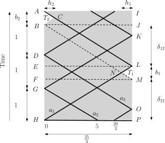
Figure 4: Three agents each with a speed of $5$ patrolling a fence of length $25/3$; their start positions are $0$, $5$, and $20/3$, respectively. Figure is not to scale.

Lemma 2.

Consider a segment of length $L=\frac{25}{3}$ such that three agents $a_{1},a_{2},a_{3}$ are patrolling perpetually each with speed of $5$ and generating an alternating sequence of uncovered triangles $T_{2},T_{1},T_{2},T_{1},\ldots$, as shown in the position-time diagram in Fig. 4. Denote the vertical distances between consecutive occurrences of $T_{1}$ and $T_{2}$ by $\delta_{12}$ and between consecutive occurrences of $T_{2}$ and $T_{1}$ by $\delta_{21}$. Denote the bases of $T_{1}$ and $T_{2}$ by $b_{1}$ and $b_{2}$ respectively, and the heights of $T_{1}$ and $T_{2}$ by $h_{1}$ and $h_{2}$ respectively. Then

1. $\frac{10}{3}$ is a period of the schedule.

2. $T_{1}$ and $T_{2}$ are congruent; further, $b_{1}=b_{2}=\frac{1}{3}$, $\delta_{12}=\delta_{21}=\frac{4}{3}$, and $h_{1}=h_{2}=\frac{5}{6}$.

Proof.

(i) Observe that $a_{1}$, $a_{2}$ and $a_{3}$ reach the left endpoint of the segment at times $2(25/3)/5=10/3$, $5/5=1$, and $(25/3+5/3)/5=2$, respectively. During the time interval $[0,10/3]$, each agent traverses the distance $2L$ and the positions and directions of the agents at time $t=10/3$ are the same as those at time $t=0$. Hence $10/3$ is a period for their schedule.

(ii) Since $AL\parallel BM$ and $AB\parallel LM$, we have $b_{1}=b_{2}$. Since $L$ is the midpoint of $IP$, we have $\delta_{12}+b_{2}=\delta_{21}+b_{1}$, thus $\delta_{12}=\delta_{21}$. Since all the agents have same speed, $5$, all the trajectory line segments in the position-time diagram have the same slope, $1/5$. Hence $\angle{BAC}=\angle{ABC}=\angle{MLN}=\angle{LMN}$. Thus, $T_{1}$ is similar to $T_{2}$. Since $b_{1}=b_{2}$, $T_{1}$ is congruent to $T_{2}$, and consequently $h_{1}=h_{2}$.

Put $b=b_{1}$, $h=h_{1}$, and $\delta=\delta_{12}$. Recall from (i) that $|AH|=10/3$. By construction, we have $|BD|=1$, thus $|BH|=|BD|+|DG|+|GH|=1+1+1=3$. We also have $|AH|=b+|BH|$, thus $b=10/3-3=1/3$. Since $L$ is the midpoint of $IP$, we have $\delta+b=5/3$, thus $\delta=5/3-b=4/3$.

Let $x(N)$ denote the $x$-coordinate of point $N$; then $x(N)+h=25/3$. To compute $x(N)$ we compute the intersection of the two segments $HL$ and $BM$. We have $H=(0,0)$, $L=(25/3,5/3)$, $B=(0,3)$, and $M=(25/3,4/3)$. The equations of $HL$ and $BM$ are $HL$ : $x=5y$ and $BM$ : $x+5y=15$, and solving for $x$ yields $x=15/2$, and consequently $h=25/3-15/2=5/6$. ∎

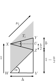
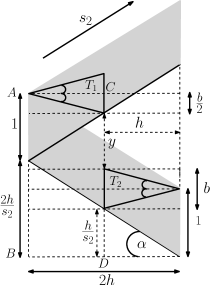
Figure 5: Left: agent covering an uncovered triangle $T_{i}$. Right: agent covering an alternate sequence of congruent triangles $T_{1},T_{2}$, with collinear bases.

Lemma 3.

(i) Let $s_{1}$ be the speed of an agent needed to cover an uncovered isosceles triangle $T_{i}$; refer to Fig. 5 (left). Then $s_{1}=\frac{h}{1-b/2}$, where $b<1$ and $h$ are the base and height of $T_{i}$, respectively.

(ii) Let $s_{2}$ be the speed of an agent needed to cover an alternate sequence of congruent isosceles triangles $T_{1},T_{2}$ with bases on same vertical line; refer to Fig. 5 (right). Then $s_{2}=\frac{h}{3b/2+y-1}$ where $y$ is the vertical distance between the triangles, $b<1$ is the base and $h$ is the height of the congruent triangles.

Proof.

(i) In Fig. 5 (left), $\tan\alpha=1/s_{1}$, $|UZ|=b/2$, hence $|VZ|=1-b/2$. Also, $\frac{|VZ|}{|WV|}=\tan\alpha=\frac{1-b/2}{h}=\frac{1}{s_{1}}$, which yields $s_{1}=\frac{h}{1-b/2}$.

(ii) In Fig. 5 (right), $|AB|=1+\frac{2h}{s_{2}}$. Also, $|CD|=\frac{b}{2}+y+b+\frac{h}{s_{2}}$. Equating $1+\frac{2h}{s_{2}}=\frac{3b}{2}+y+\frac{h}{s_{2}}$ and solving for $s_{2}$, we get $s_{2}=\frac{h}{3b/2+y-1}$. ∎

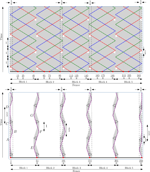
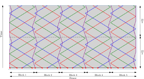
Figure 6: Top: iterative construction with $5$ blocks; each block has three agents with speed $5$. Middle: six agents with speed $1$. Bottom: patrolling strategy for $5$ blocks using $21$ agents for two time periods (starting at $t=1/3$ relative to Fig. 4); the block length is $25/3$ and the time period is $10/3$.

Theorem 3.

For every integer $x\geq 2$, there exist $k=4x+1$ agents with $\sum_{i=1}^{k}v_{i}=16x+1$ and a guarding schedule for a segment of length $25x/3$. Alternatively, for every integer $x\geq 2$ there exist $k=4x+1$ agents with suitable speeds $v_{1},\ldots,v_{k}$, and a guarding schedule for a unit segment that achieves idle time at most $\frac{48x+3}{50x}\,\frac{2}{\sum_{i=1}^{k}v_{i}}$. In particular, for every $\varepsilon>0$, there exist $k$ agents with suitable speeds $v_{1},\ldots,v_{k}$, and a guarding schedule for a unit segment that achieves idle time at most $\left(\frac{24}{25}+\varepsilon\right)\,\frac{2}{\sum_{i=1}^{k}v_{i}}$.

Proof.

Refer to Fig. 6. We use a long fence divided into $x$ blocks; each block is of length $25/3$. Each block has 3 agents each of speed 5 running in zig-zag fashion. Consecutive blocks share one agent of speed $1$ which covers the uncovered triangles from the trajectories of the zig-zag agents in the position-time diagram. The first and the last block use two agents of speed $1$ not shared by any other block. The setting of these speeds is explained below.

From Lemma 2(ii), we conclude that all the uncovered triangles generated by the agents of speed 5 are congruent and their base is $b=1/3$ and their height is $h=5/6$. By Lemma 3(i), we can set the speeds of the agents not shared by consecutive blocks to $s_{1}=\frac{5/6}{1-1/6}=1$. Also, in our strategy, Lemma 2(ii) yields $y=\delta=4/3$. Hence, by Lemma 3(ii), we can set the speeds of the agents shared by consecutive blocks to $s_{2}=\frac{5/6}{1/2+4/3-1}=1$.

In our strategy, we have 3 types of agents: agents running with speed 5 as in Fig. 6 (top), unit speed agents not shared by 2 consecutive blocks and unit speed agents shared by two consecutive blocks as in Fig. 6 (middle). By Lemma 2(i), the agents of first type have period $10/3$. In Fig. 6 (middle), there are two agents of second type and both have a similar trajectory. Thus, it is enough to verify for the leftmost unit speed agent. It takes $5/6$ time from $A$ to $B$ and again $5/6$ time from $B$ to $C$. Next, it waits for $5/3$ time at $C$. Hence after $5/6+5/6+5/3=10/3$ time, its position and direction at $D$ is same as that at $A$. Hence, its time period is $10/3$. For the agents of third type, refer to Fig. 6 (middle): it takes $10/6$ time from $E$ to $F$ and $10/6$ time from $F$ to $G$. Thus, arguing as above, its time period is $10/3$. Hence, overall, the time period of the strategy is $10/3$.

For $x$ blocks, we use $3x+(x+1)=4x+1$ agents. The sum of all speeds is $5(3x)+1(x+1)=16x+1$ and the total fence length is $\frac{25x}{3}$. The resulting ratio is $\rho=\frac{16x+1}{2}/\frac{25x}{3}=\frac{48x+3}{50x}$. For example, when $x=2$ we reobtain the bound of Kawamura and Kobayashi [9] (from their 2nd example), when $x=39,\rho=\frac{100}{104}$ and further on, $\rho\underset{x\to\infty}{\longrightarrow}\,\frac{24}{25}$. Thus an idle time of at most $\left(\frac{24}{25}+\varepsilon\right)\,\frac{2}{\sum_{i=1}^{k}v_{i}}$ can be achieved for every given $\varepsilon>0$, as required. ∎

Acknowledgements.

We sincerely thank Akitoshi Kawamura for generously sharing some technical details concerning their patrolling algorithms. We also express our satisfaction with the software package JSXGraph, Dynamic Mathematics with JavaScript, used in our experiments.

References

- [1] N. Agmon, S. Kraus, and G. A. Kaminka, Multi-robot perimeter patrol in adversarial settings, in Proc. International Conference on Robotics and Automation (ICRA 2008), IEEE, 2008, pp. 2339–2345.
- [2] J. Barajas and O. Serra, The lonely runner with seven runners, Electronic Journal of Combinatorics 15 (2008), R48.
- [3] T. Bohman, R. Holzman, and D. Kleitman, Six lonely runners, Electronic Journal of Combinatorics 8 (2001), R3.
- [4] Y. Chevaleyre, Theoretical analysis of the multi-agent patrolling problem, in Proc. International Conference on Intelligent Agent Technology (IAT 2004), IEEE, 2004, pp. 302–308.
- [5] H. Choset, Coverage for robotics—a survey of recent results, Annals of Mathematics and Artificial Intelligence 31 (2001), 113–126.
- [6] T. W. Cusick, View-obstruction problems, Aequationes Math. 9 (1973), 165–170.
- [7] J. Czyzowicz, L. Gasieniec, A. Kosowski, and E. Kranakis, Boundary patrolling by mobile agents with distinct maximal speeds, in Proc. 19th European Symposium on Algorithms (ESA 2011), LNCS 6942, Springer, 2011, pp. 701–712.
- [8] Y. Elmaliach, N. Agmon, and G. A. Kaminka, Multi-robot area patrol under frequency constraints, in Proc. International Conference on Robotics and Automation (ICRA 2007), IEEE, 2007, pp. 385–390.
- [9] A. Kawamura and Y. Kobayashi, Fence patrolling by mobile agents with distinct speeds, in Proc. 23rd International Symposium on Algorithms and Computation (ISAAC 2012), LNCS 7676, Springer, 2012, pp. 598–608.
- [10] A. Machado, G. Ramalho, J. D. Zucker, and A. Drogoul, Multi-agent patrolling: an empirical analysis of alternative architectures, 3rd International Workshop on Multi-Agent-Based Simulation, Springer, 2002, pp. 155–170.
- [11] J. M. Wills, Zwei Sätze über inhomogene diophantische Approximation von Irrationalzahlen, Monatsch. Math. 71 (1967), 263–269.