Dynamics of localized and patterned structures in the Lugiato-Lefever equation determine the stability and shape of optical frequency combs

Abstract

It has been recently uncovered that coherent structures in microresonators such as cavity solitons and patterns are intimately related to Kerr frequency combs. In this work, we present a general analysis of the regions of existence and stability of cavity solitons and patterns in the Lugiato-Lefever equation, a mean-field model that finds applications in many different nonlinear optical cavities. We demonstrate that the rich dynamics and coexistence of multiple solutions in the Lugiato-Lefever equation are of key importance to understanding frequency comb generation. A detailed map of how and where to target stable Kerr frequency combs in the parameter space defined by the frequency detuning and the pump power is provided. Moreover, the work presented also includes the organization of various dynamical regimes in terms of bifurcation points of higher co-dimension in regions of parameter space that were previously unexplored in the Lugiato-Lefever equation. We discuss different dynamical instabilities such as oscillations and chaotic regimes.

I Introduction

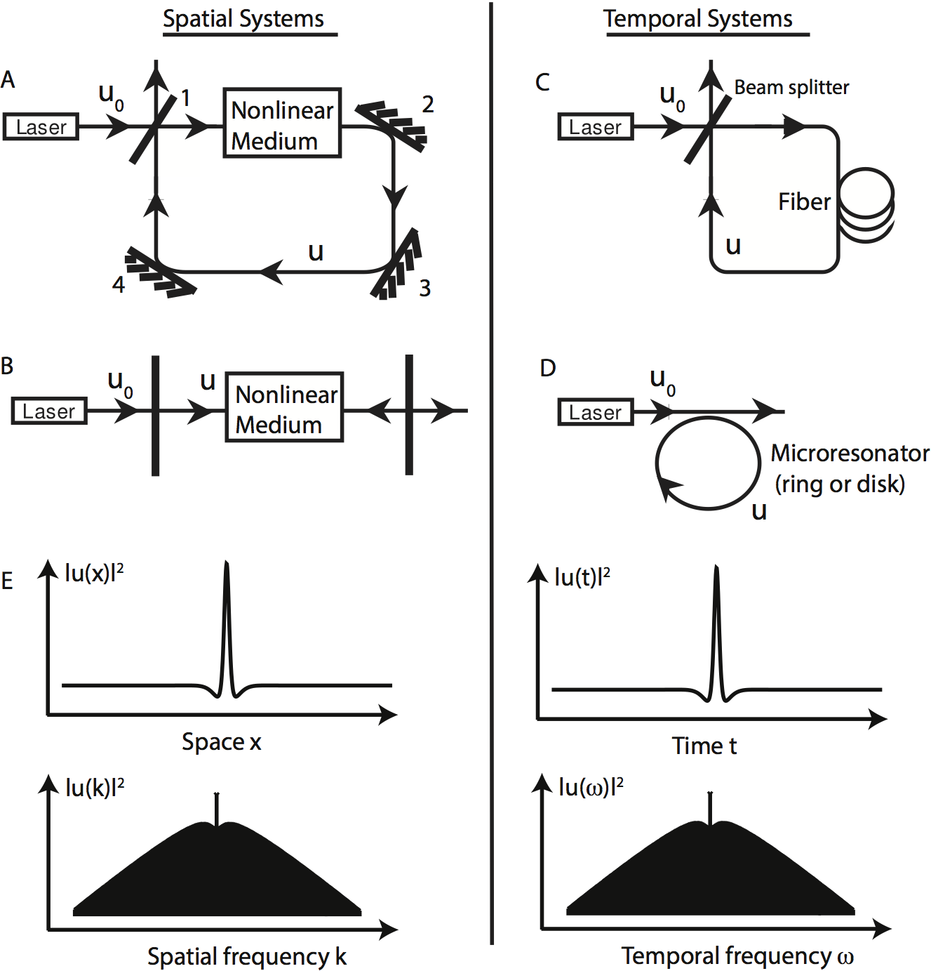
Figure 1: Different set-ups where the mean field $u$ is described by the Lugiato-Lefever equation (LLE). A. A ring cavity partially filled with a nonlinear medium. Mirror 1 partially transmits the input beam $u_{0}$, while mirrors 2-4 are completely reflecting. B. A Fabry-Perot resonator filled with a nonlinear medium. C. A nonlinear all-fiber cavity. D. A microresonator where the cavity can be either a ring or a disk. E. A sketch of a localized structure, both in the time (spatial) domain and in the corresponding Fourier domain.

Optical frequency combs can be used to measure light frequencies and time intervals more easily and precisely than ever before Cundiff et al. (2008), opening a large avenue for applications. Traditional frequency combs are usually associated with trains of evenly spaced, very short pulses. More recently, a new generation of comb sources has been demonstrated in compact high-Q optical microresonators with a Kerr nonlinearity pumped by continuous-wave laser light Del’Haye et al. (2007). These combs are now referred to as Kerr frequency combs and have attracted a lot of interest in the last few years Kippenberg et al. (2011). Interestingly, it has been demonstrated that Kerr frequency combs can be modeled in a way that is strongly reminiscent of temporal cavity solitons (CSs) in nonlinear cavities Coen et al. (2013); Coen and Erkintalo (2013); Chembo and Menyuk (2013). Temporal CSs have been experimentally studied in fiber resonators Leo et al. (2010) and their description is based on a now classical equation, the Lugiato-Lefever equation (LLE), that describes pattern formation in optical systems Lugiato and Lefever (1987).

Lugiato and Lefever, in 1987, introduced the mean-field model of nonlinear optical cavities, in which alternation of propagation around the cavity with coherent addition of an input field is replaced by a single partial differential equation with a driving term Lugiato and Lefever (1987). The LLE is applicable to different types of cavities, as shown in Figure 1. It was originally derived to describe a ring cavity or a Fabry-Perot resonator with a transverse spatial extension and partially filled with a nonlinear medium Lugiato and Lefever (1987) (see Figures 1A-B). The LLE can also be used in the context of single-mode fiber cavities (see Figure 1C) Leo et al. (2010). In this case, the spatial coordinate in the LLE for a spatially extended cavity with diffraction is replaced by a time coordinate to model chromatic dispersion of light in the longitudinal (temporal) direction. Finally, more recently, the LLE has been applied to microresonators (see Figure 1D) in the context of optical frequency combs Matsko et al. (2011); Coen et al. (2013); Coen and Erkintalo (2013); Chembo and Menyuk (2013).

The interplay between diffraction and/or dispersion and nonlinearity can lead to the formation of complex spatio-temporal structures inside the cavity, such as patterned and localized solutions (see Figure 1E). In the cavities presented in Figures 1A-B, a spatially localized bright light spot embedded in a homogeneous background of light has been shown to exist at the output of the resonator Barland et al. (2002). Such structures, localized in space, are also known as spatial cavity solitons (CSs). Similarly, in the cavities presented in Figures 1C-D, a stable structure that is localized in time can exist, also known as temporal cavity solitons Leo et al. (2010). A sketch of such a localized structure, both in the time (spatial) domain as well as in the corresponding Fourier domain, is shown in Figure 1E.

The formation and stability of patterns and CSs have been theoretically studied in great detail in the LLE, both in a one dimensional (1D) and a two dimensional (2D) setting Lugiato and Lefever (1987); McSloy et al. (2002); Scroggie et al. (1994); Gomila et al. (2007); Firth et al. (2002); Gomila et al. (2007). The theory developed for CSs in the LLE was mainly motivated by the potential application of spatial CSs as information carriers in all-optical memories Barland et al. (2002); McSloy et al. (1990). Recent experimental observations of 1D temporal CSs in fiber resonators Leo et al. (2010) have renewed the interest in the LLE. This interest was further strengthened when it was demonstrated that the LLE can also be used to efficiently model Kerr frequency combs and that these were found, in some conditions, to be closely related to temporal CSs present inside the cavity Coen et al. (2013); Coen and Erkintalo (2013); Chembo and Menyuk (2013). Experimental evidence of CSs in microresonators has emerged shortly after Herr et al. (0733). The theory that has been developed for spatial CSs can thus potentially provide important information about the properties of Kerr frequency combs. In 1D, CSs have mainly been studied for lower values of the cavity frequency detuning, where they were shown to be always stable Gomila et al. (2007). However, in the context of Kerr frequency combs, experiments are often carried out at relatively high pump power Del’Haye et al. (2007); Foster et al. (2011). Because of the Kerr-induced tilt of the cavity resonance, the detuning, which is measured from the center of the linear (cold) resonance, is correspondingly large. Only a few recent studies have been reported in this regime Coen and Erkintalo (2013); Turaev et al. (2012); Leo et al. (2013a). In particular, a fiber cavity experiment has demonstrated that CSs can display periodic oscillations, and preliminary numerical analysis have also revealed various chaotic regimes Leo et al. (2013a).

In this work, we aim to realize two goals: i) to interpret how various coherent structures in microresonators, such as patterns and solitons, are intimately related to different types of Kerr frequency combs; ii) to expand the study of the LLE to operating regimes that will prove to be of key importance for frequency comb generation, but so far have not been much explored. Such a detailed analysis of the unfolding of the rich dynamical behavior of the LLE for higher values of the detuning will also prove to be of fundamental interest for researchers working in the field of dissipative solitons.

The organization of this paper will be as follows. In Section II, we will introduce the Lugiato-Lefever model in more detail. In Section III we will discuss the coexistence of multiple solutions, such as homogeneous solutions, patterned solutions and localized solutions. We will show that all these structures are organized in a so-called snaking diagram and will discuss its importance in the context of frequency comb generation. In Section IV, we consider how the homogeneous state can connect to a patterned state and back, thus forming CSs. For transverse systems, this is referred to as the spatial dynamics and we will keep this terminology for combs for which the spatial coordinate is replaced by a longitudinal (temporal) variable. This study provides us with essential information about the location in parameter space where stable CSs and frequency combs can be found. In Section V the dynamical behavior of single-peak CSs and their corresponding frequency combs is studied in the parameter space defined by the cavity detuning and the pump power. Finally, we draw our conclusions in the final Section VI.

II The Lugiato-Lefever equation

The LLE is a prototype model describing an optical cavity filled with a nonlinear Kerr medium as derived by Lugiato and Lefever in order to study pattern formation in this system Lugiato and Lefever (1987). Later studies have then demonstrated the existence of CSs in the LLE McSloy et al. (2002); Scroggie et al. (1994); Gomila et al. (2007); Firth et al. (2002); Gomila et al. (2007). The LLE was originally obtained through a mean-field approximation, describing the dynamics of the slowly varying amplitude of the electromagnetic field $u(\varphi,t)$ in the paraxial limit, where $\varphi=x$ is the spatial coordinate transverse to the propagation direction. Here we consider only one transverse dimension. The time evolution of the electric field over many cavity roundtrips can then be described as follows after a suitable rescaling of the variables Lugiato and Lefever (1987):

$$\partial_{t}u=-(1+i\theta)u+i|u|^{2}u+u_{0}+i\partial_{\varphi}^{2}u\,.$$ (1)

The first term on the right-hand side describes cavity losses (the system is dissipative by nature); $u_{0}$ is the amplitude of the homogeneous (plane wave) input field or pump; $\theta$ measures the cavity frequency detuning between the frequency of the input pump and the nearest cavity resonance; $\partial_{\varphi}^{2}$ models diffraction; and the sign of the cubic term is set so that it corresponds to the self-focusing case. In the case of a fiber resonator or a whispering-gallery-mode (WGM) microresonator, the LLE still holds, but the input field $u_{0}$ is to be interpreted as the amplitude of the continuous-wave pump beam while the field $u(\varphi,t)$ is now function of two time scales, with $\varphi=\tau$ a time coordinate — also known as fast time — in the frame moving with the group velocity Leo et al. (2010); Coen et al. (2013); Coen and Erkintalo (2013). The spatial derivatives are thus replaced by time derivatives $\partial_{\varphi}^{2}u=\partial_{\tau}^{2}u$, and the sign of this term is such that one has anomalous dispersion. Note that in our study here, we only consider second-order dispersion. Several works have also studied the influence of higher order dispersion on the dynamics of dissipative structures in the LLEGelens et al. (2008); Leo et al. (2013b); Tlidi and Gelens (2010). In the case of WGM microresonators, the LLE has also been shown to remain valid when replacing the coordinate $\varphi$ by the resonator’s azimuthal angle Chembo and Menyuk (2013).

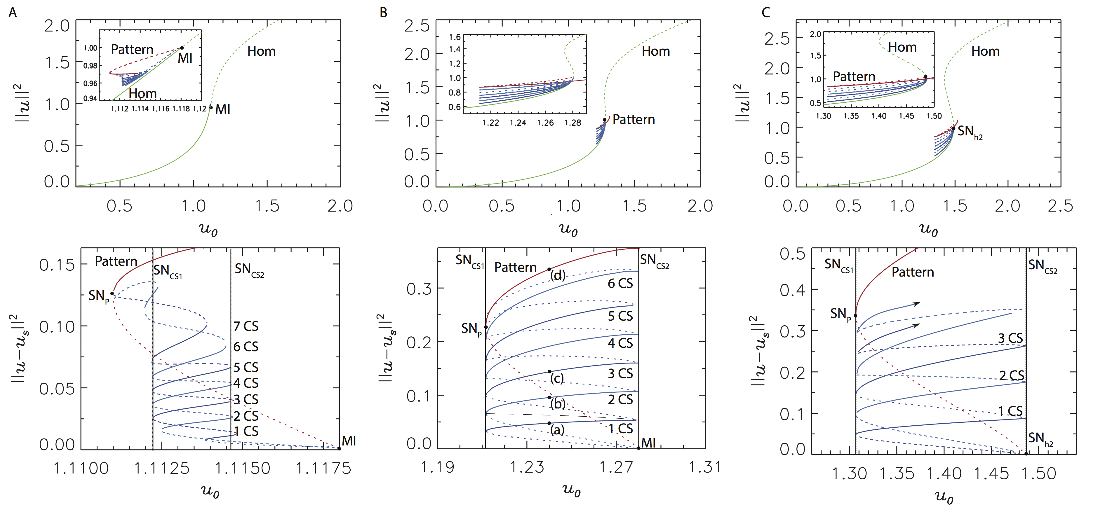
Figure 2: (Color online) Various solution branches of the LLE as function of the pump $u_{0}$ for different values of the detuning $\theta$ [$\theta=1.5$ (A), $\theta=1.8$ (B), $\theta=2.1$ (C)]. The (green) line denoted by “Hom” shows the homogeneous steady states (HSS) solutions of Eq. (1), where the inset shows a zoom of the region around the modulational instability (MI). A patterned branch (red curve, denoted “Pattern”) is created subcritically in MI. The bottom panels show a more detailed picture of the snaking region where CSs (blue curve) exist, plotting the energy of the solution after removal of the homogeneous background. The snaking region is located between two other saddle-node bifurcations, called $\mathrm{SN}_{\mathrm{CS}1,2}$. All solid (dotted) lines correspond to stable (unstable) solutions. The dots denoted by (a)–(d) in panel B correspond to solutions of which the profile is shown in Figure 4.

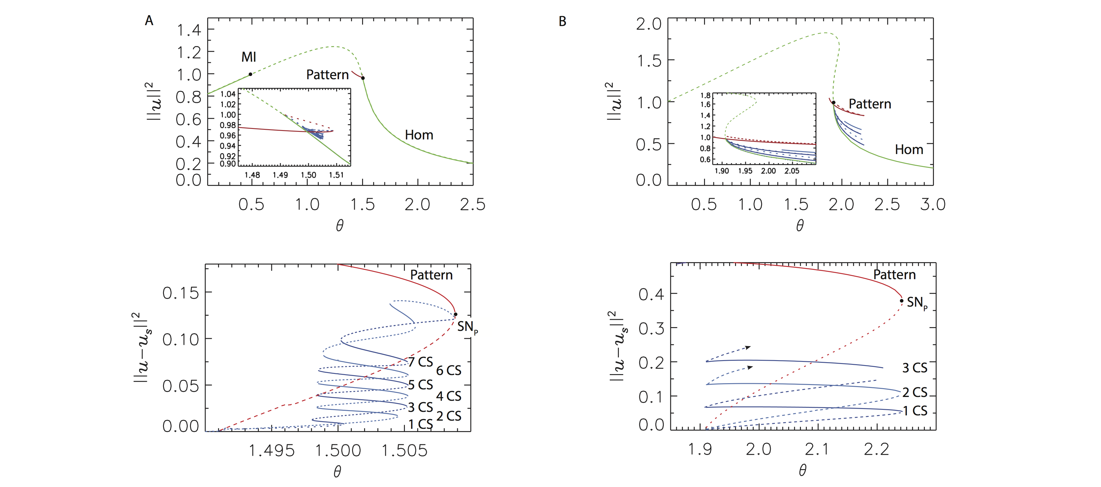
Figure 3: (Color online) Same as Figure 2 but as function of the detuning $\theta$ for different values of the pump $u_{0}$ [$u_{0}=1.114$ (A), $u_{0}=1.35$ (B)].

The homogeneous steady state (HSS) solutions $u_{s}$ of the LLE (1) are easily found by setting all derivatives to be zero:

$$I_{s}[1+(\theta-I_{s})^{2}]=I_{0}\,.$$ (2)

The above equation is the classic cubic equation (S-shape response) of dispersive optical bistability, with $I_{s}=|u_{s}|^{2}$ and $I_{0}=|u_{0}|^{2}$. For $\theta<\sqrt{3}$, only one homogeneous solution exists, hence the system is monostable. In the context of spatial CSs, this monostable regime has been studied in great detail Lugiato and Lefever (1987); McSloy et al. (2002); Scroggie et al. (1994); Gomila et al. (2007); Firth et al. (2002); Gomila et al. (2007). Much less analysis has been done when $\theta>\sqrt{3}$. In this case, for a range of input intensities $I_{0}$ Eq. (2) has three homogeneous solutions, out of which one is a saddle solution. Hence the system is often called to be bistable. In this bistable region much more complex dynamics are observed in the LLE Leo et al. (2013a).

One can easily show the existence of two HSSs analytically by looking for the points where the derivative $\partial I_{0}/\partial I_{s}$ is equal to zero,

$$\frac{\partial I_{0}}{\partial I_{s}}=1+(\theta-I_{s})^{2}-2(\theta-I_{s})I_{s}=0\text{ .}$$ (3)

The solutions to this equation give the turning points of the bistable response, also known as the saddle-node (SN) bifurcations of the HSSs:

$$I_{s}^{\mathrm{SN}_{h1,2}}=\frac{2\theta}{3}\pm\frac{1}{3}\sqrt{\theta^{2}-3}\text{ .}$$ (4)

It is clear that for $\theta^{2}<3$ there are no turning points (see Figure 2A), while for $\theta^{2}>3$ there are two, $\mathrm{SN}_{h1,2}$, and the system is bistable (see Figures 2B-C). Figures 2A-C are plotted versus the input power for selected detunings while Figs. 3A-B presents similar plots but as a function of detuning for selected pump powers. This second set of plots may be more relevant to the microresonator Kerr frequency comb context, in which the pump laser frequency is used as an important control parameter and for which thermal effects also strongly affect the detuning.

Analyzing the linear stability of the HSS to perturbations of the form $\exp{(ik\varphi+\sigma t)}$ Scroggie et al. (1994), one finds that, for $\theta<\sqrt{3}$, the HSS loses its stability at $I_{s}=1$ with critical wavenumber $k_{c}=\sqrt{2-\theta}$ at which point a patterned solution is created either supercritically ($\theta<41/30$) or subcritically ($\theta>41/30$) Scroggie et al. (1994). In the bistable regime ($\theta>\sqrt{3}$), one can differentiate two different cases: $\sqrt{3}<\theta<2$, in which, as before, the MI occurs at $I_{s}=1$, and $\theta>2$ in which the critical wavenumber is zero and the HSS is stable all the way to $\mathrm{SN}_{h2}$. In the latter case if $I_{s}$ is increased above $I_{s}^{\mathrm{SN}_{h2}}$ the HSS jumps to the upper branch, but the upper branch HSS has always a wide range of unstable wavenumbers, whose growth leads to a spatio-temporal chaotic regime called optical turbulence Mitschke et al. (1996); Gomila and Colet (2003).

In this work we will show how localized and patterned solutions are organized in both the monostable and the bistable regime, putting more emphasis on the bistable region as the monostable one has already been studied in depth. A typical example of the bifurcation diagram of the homogeneous solutions is shown in Figures 2A-C for values of the detuning $\theta$ in each characteristic region: $\theta<\sqrt{3}$, $\sqrt{3}<\theta<2$, and $\theta>2$. In the bistable region shown in Figures 2B-C, there exists a small region of input powers where the two homogeneous solutions coexist. The homogeneous solution with the highest intensity is always unstable in Eq. (1). A pattern is created subcritically at the modulational instability for $\theta<2$ such that a stable pattern can coexist with the stable homogeneous solution in a certain range of parameters. For $\theta>2$, although the system goes directly to optical turbulence above $\mathrm{SN}_{h,2}$, stable periodic patterns persist below threshold. Such coexistence is known to potentially give rise to localized structures, such as CSs, as will be discussed in the next Section.

III Cavity solitons, patterns and frequency combs

The bottom panels in Figures 2A-C and 3A-B show a zoom of the region where a subcritical branch of spatially periodic states (red) coexists with a stable homogeneous solution (green). For $\theta>41/30$ the pattern branch is unstable at its point of origin (MI), but acquires stability at finite amplitude at a saddle-node bifurcation $\mathrm{SN}_{P}$. In addition, it is known that there are two branches of CSs (blue) that bifurcate from the homogeneous solution simultaneously with the periodic states, and do so likewise subcritically Gomila et al. (2007). These states are therefore also initially unstable. When followed numerically these states become better and better localized and once their amplitude and width become comparable to the amplitude and wavelength of the periodic state, these CS states begin to grow in spatial extent by adding peaks symmetrically on either side, thereby forming bound states of CSs. In a bifurcation diagram this growth is associated with back and forth oscillations across a pinning interval [$\mathrm{SN}_{\mathrm{CS}1}-\mathrm{SN}_{\mathrm{CS}2}$]. This behavior is known as homoclinic snaking Champneys (1998); Hunt et al. (2000); Knobloch and Wagenknecht (2005); Burke and Knobloch (2006); Kozyreff and Chapman (2006), and is associated with repeated gain and loss of stability of the associated localized structures. This snaking structure has been experimentally verified for spatial CSs in a semiconductor-based optical system Barbay et al. (2008).

Figure 2 shows a clear difference in the location of the pinning interval [$\mathrm{SN}_{\mathrm{CS}1}-\mathrm{SN}_{\mathrm{CS}2}$] when transitioning from the monostable (Figure 2A) to the bistable region of operation (Figures 2B-C). For $\theta<\sqrt{3}$, the pinning interval where CSs can be found spans only a part of the region of coexistence between the stable pattern and the stable homogeneous solution, while for increasing values of the detuning in the bistable region ($\theta>\sqrt{3}$) the pinning interval quickly spans this entire region of coexistence. Another clear trend is that the CSs exist over a much broader range of values of the input amplitude $u_{0}$ and detuning $\theta$ as both $u_{0}$ and $\theta$ are increased in the bistable region. This evolution will be discussed in more detail in the next Section IV. We remark that for increasing values of the detuning $\theta$ it becomes increasingly difficult to numerically track the CS snaking branches. We believe this is not a numerical artifact, but rather that the snaking structure becomes more complex for $\theta>2$ hindering the numerical tracking of these CS branches (although solutions with multiple CSs seem to persist). Understanding the detailed snaking structure for high values of $\theta$ is beyond the scope of this paper and it will addressed elsewhere.

In Figure 4, we show typical profiles of the stable CSs that exist in an optical cavity described by the LLE. As mentioned before, there exist two branches of CSs that coexist in the pinning region. One branch corresponds to CS states with an odd amount of peaks, while the other branch contains the solutions with an even amount of peaks. A typical one-peak CS is shown in Figure 4(a). In a fiber resonator or microresonator this solution would correspond to a time-localized pulse circulating in the cavity. Such a light pulse corresponds to a stable smooth frequency comb in the corresponding frequency domain, as shown in the panel on the right hand side. The distance between all frequency modes is given by the free-spectral-range $\mathrm{FSR}=1/L$, where $L$ is the cavity length, while the exact shape of the frequency comb is determined by the Fourier transform of the profile of the CS itself. This equivalence has also been studied in Refs. Coen et al. (2013); Coen and Erkintalo (2013); Chembo and Menyuk (2013). Solutions with two peaks and three peaks are plotted in panels (b) and (c), with the corresponding frequency combs. It can be seen that the effect of adding extra peaks is to introduce an extra modulation of the frequency comb. The multiple peaks of CS bound states can only coexist at well-defined separation distances $d$ between them, determined by the typical wavelength of the oscillatory tails of the CS peaks Kozyreff and Gelens (2011). This separation distance $d$ therefore also determines the modulation distance $1/d$ observed in the frequency comb. The modulation depth becomes more pronounced as more and more peaks are added to the solution.

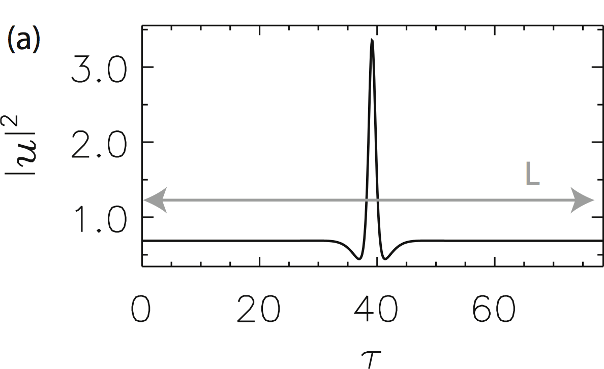
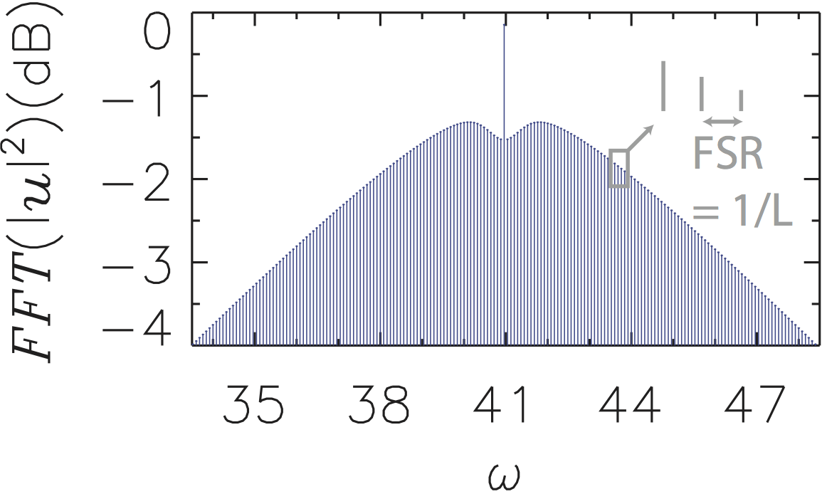
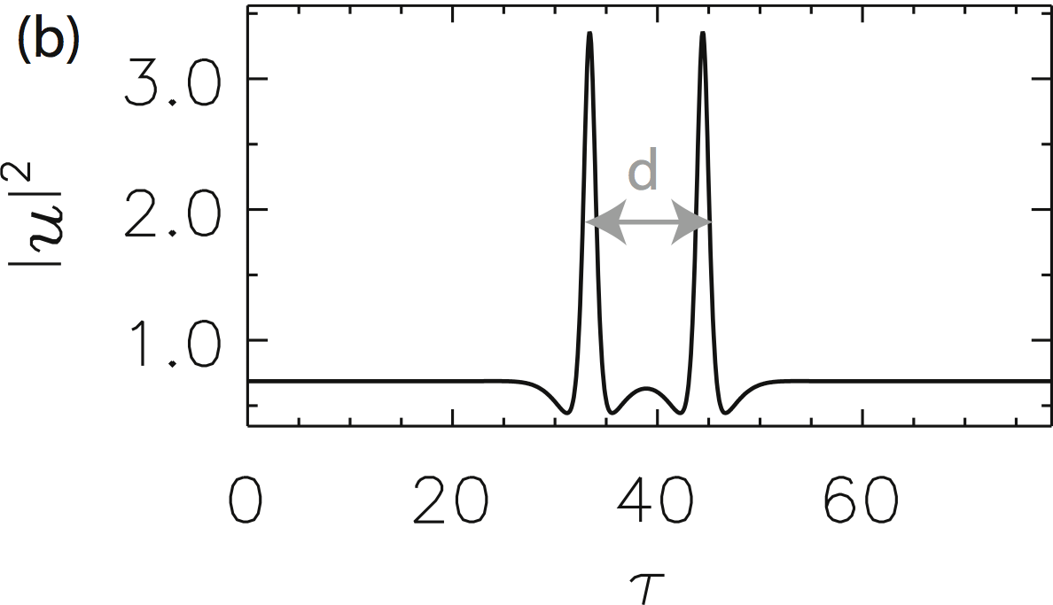
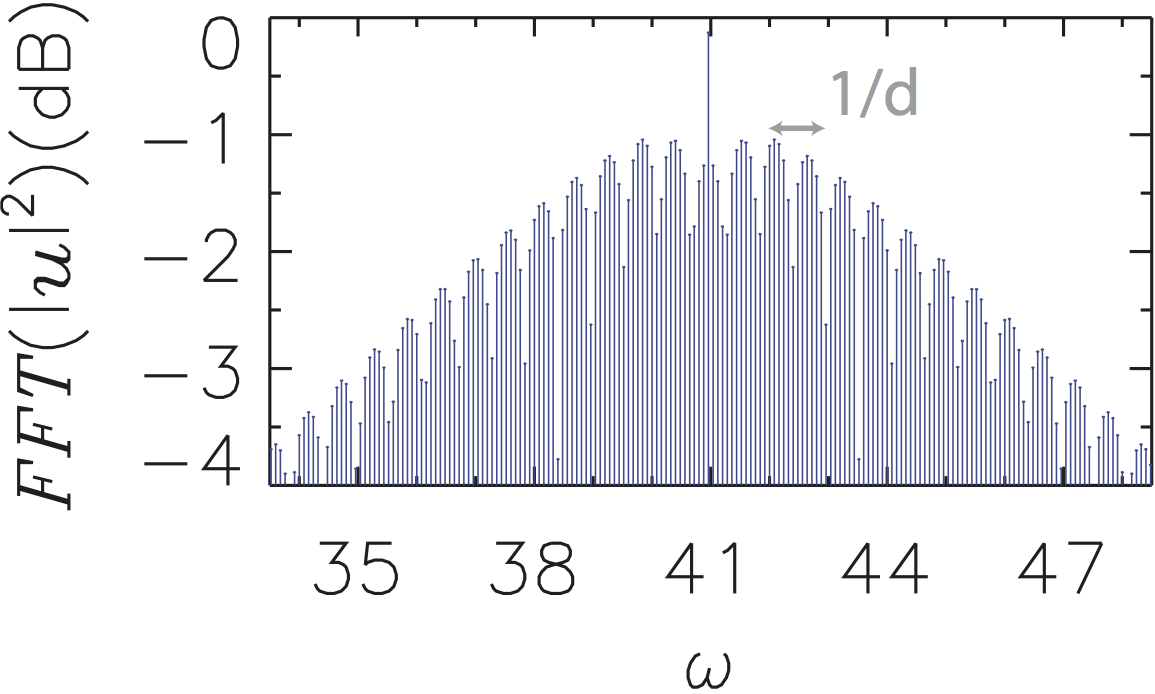
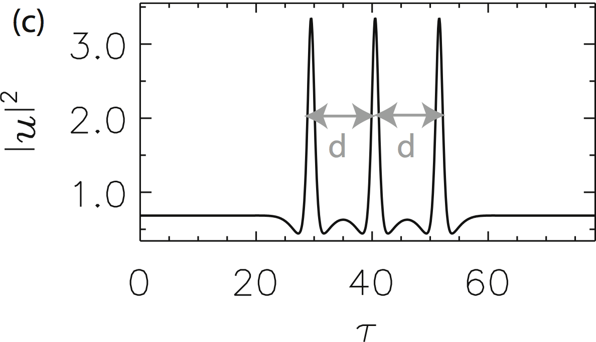
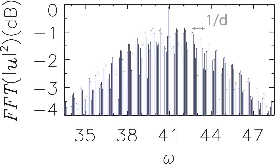
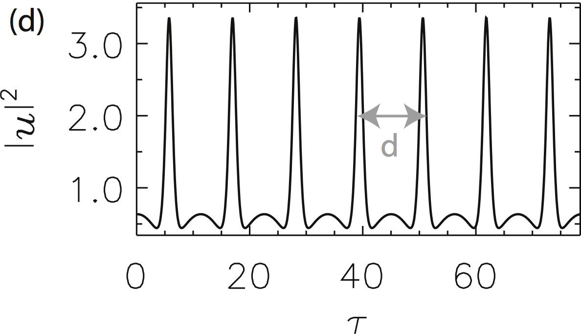
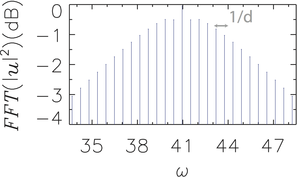
Figure 4: Profiles of a single CS (a), two CSs (b), three CSs (c) and a pattern (d) on the left hand side, with their corresponding frequency combs on the right hand side. The system parameters are: $\theta=1.8$, the free spectral range $\mathrm{FSR}=1/L=0.08$ and the number of discretization points was taken to be $N=512$.

In an infinite system (unbounded domain) CS peaks can be added indefinitely such that the two snaking branches in principle continue indefinitely. However, realistic systems are always bounded. In this case the CS branches cannot endlessly snake back and forth. Instead the snaking structure is truncated when the width of the localized patterns consisting of multiple CSs approaches the domain size. In the case of fiber resonators or microresonators, periodic boundary conditions apply and the system is finite as determined by the size of the fiber loop, ring or disk resonator. In such a finite system the CS branches in the snaking region are generally found to connect to a branch of patterned solutions. This is also the case here, as can be seen in Figure 2. Moreover the branches of small amplitude CSs (i.e. the first unstable branch of single CSs) no longer bifurcate from the HSS but now bifurcate in a secondary bifurcation on the primary branch of the pattern solutions A. Bergeon and Mercader (2008). An example of a patterned solution with 7 peaks is shown in Figure 4(d). All frequency modes present in the corresponding frequency comb are now separated by $1/d$ (or equivalently 7 FSR units). Although we have used the same distance $d$ to denote the separation between various peaks in the pattern, we remark that this should not necessarily be the case, as this might vary a bit depending on the exact cavity length. We note also that CSs with $L/d-1$ peaks can be interpreted as one missing cell, or hole, in a periodic pattern.

It is clear from Figure 2 that nonlinear optical cavities described by the LLE admit many stable and unstable localized and patterned solutions for the same set of system parameters (such as the frequency detuning and the pump power). Having such a highly multistable landscape has important consequences if one aims at creating a stable Kerr frequency comb. Every stable solution of the LLE has its own basin of attraction in the infinite dimensional phase space. Choosing the correct initial conditions and/or writing process will thus be essential to target the structure one would like to have in the nonlinear resonator. Minor changes might result in obtaining a homogeneous solution, a single CS, a group of CSs or a pattern; all of which correspond to different frequency combs.

In the next Section, we will analyze the spatial dynamics of the homogeneous steady state solutions as this will provide valuable information about where one can expect stable CSs to be found. We will verify this theory in Section V and will examine the rich temporal dynamics of CSs, which is also reflected in the corresponding frequency combs.

IV Spatial dynamics

The solutions $u$ of the LLE in which we are interested, namely CSs and localized patterns (groups of CSs), are stationary solutions of (1) (a PDE), i.e. they are such that $\partial_{t}u=0$ . Under this condition, Eq. (1) can be simplified to a special dynamical system of first order real ODEs in which space/fast-time, $\varphi$ in our case, takes the role usually played by time (see, e.g. Refs. Haragus and Iooss (2011); Champneys (1998); Gomila et al. (2007); Colet et al. (6801)), namely,

$$d_{\varphi}u_{1} = u_{3}$$

$$d_{\varphi}u_{2} = u_{4}$$

$$d_{\varphi}u_{3} = u_{2}+\theta u_{1}-u_{1}I_{s}$$

$$d_{\varphi}u_{4} = -u_{1}+\theta u_{2}-u_{2}I_{s}+u_{0}\ ,$$ (5)

with $u_{1}=\mathrm{Re}(u)$, $u_{2}=\mathrm{Im}(u)$, $u_{3}=d_{\varphi}u_{1}$, $u_{4}=d_{\varphi}u_{2}$, and $I_{s}=|u|^{2}=u_{1}^{2}+u_{2}^{2}$. Bounded trajectories of this dynamical system correspond to the stationary solutions of (1). In particular, it contains all information about the stability of the stationary solutions and describes what is known as their spatial dynamics [spatial, because this technique has traditionally been applied to transverse structures]. The spatial dynamics describe also how different solutions can coexist (if at all) in the cavity and how each one connects to the other, hence revealing in which parts of the parameter space particular stationary solutions can potentially exist. Clearly, this has important practical implications for Kerr frequency combs.

The fixed points of Eqs. (5) are the HSSs $u_{s}$ of the original evolution equation (1), and their stability in space ${\varphi}$ can be analyzed by introducing the ansatz ${\color[rgb]{0,0,0}u}=u_{s}+\epsilon e^{\lambda{\varphi}}$ into Eqs.  (5) . Keeping only linear terms in (small) $\epsilon$ leads to the following condition for what are known as the spatial eigenvalues $\lambda$,

$$\lambda^{4}+(4I_{s}-2\theta)\lambda^{2}+\theta^{2}-4\theta I_{s}+3I_{s}^{2}+1=0\,.$$ (6)

An important property of the spatial dynamics is reversibility, that stems from the invariance of the LLE (1) with $\partial_{t}u=0$ under the ${\varphi}\rightarrow-{\varphi}$ transformation, and, equivalently, of Eqs. (5) under the transformation $(u_{1},u_{2},u_{3},u_{4})\rightarrow(u_{1},u_{2},-u_{3},-u_{4})$ Gomila et al. (2007). Note that this arises in the temporal Kerr comb problem ($\varphi=\tau$) because of our approximation to consider only second order dispersion. Reversibility implies that the spatial eigenvalues always come in pairs (cf. e.g. Colet et al. (6801)): each spatial eigenvalue $\lambda$ is accompanied by its counterpart $-\lambda$, and this property manifests also in that Eq. (6) is only function of $\lambda^{2}$, not of $\lambda$ alone [Eq. (6) is a biquadratic equation] . Thus, a repelling eigenvalue is accompanied by another attracting one with the same rate (repelling/attracting means that the spatial dynamics takes the field of the solution away/towards the HSS $u_{s}$).

The spatial eigenvalues can be easily obtained by solving Eq. (6), that yields,

$$\lambda=\pm\sqrt{\theta-2I_{s}\pm\sqrt{I_{s}^{2}-1}}\ .$$ (7)

These eigenvalues provide all relevant information about the HSSs, and allow to identify different regions in parameter space, in terms of the form of the leading eigenvalues, i.e. those whose real part is closer to zero. Three characteristic cases can be distinguished:

1. The eigenvalues are organized as a quartet of complex eigenvalues $\lambda=\pm q_{0}\pm ik_{0}$, such that a trajectory leaving (and approaching) the HSS presents oscillations. This is the case corresponding to label I in Figure 6 and Table 1.

2. The leading eigenvalues are a purely real doublet $\lambda=\pm q_{0}$, such that a trajectory leaving (and approaching) the HSS is monotonic (Label II in Figure 6 and Table 1).

3. The leading eigenvalues are a purely imaginary doublet $\lambda=\pm ik_{0}$, such that the HSS is temporally unstable (Labels III and IV in Figure 6 and Table 1)

Cod	$(\lambda_{1,2},\lambda_{3,4})$	Name	Label
Zero	$(\pm q_{0}\pm ik_{0})$	Double-Focus	I
Zero	$(\pm q_{1},\pm q_{2})$	Double-Saddle	II
Zero	$(\pm ik_{1},\pm ik_{2})$	Double-Center	III
Zero	$(\pm q_{0},\pm ik_{0})$	Saddle-Center	IV
One	$(\pm q_{0},0)$	Rev. Takens-Bodganov	$\mathrm{SN}_{h,2}$(RTB)
One	$(\pm ik_{0},0)$	Rev. Takens-Bodgano-Hopf	$\mathrm{SN}_{h,2}$(RTBH)
One	$(\pm q_{0},\pm q_{0})$	Belyakov-Devaney	BD
One	$(\pm ik_{0},\pm ik_{0})$	Hamiltonian-Hopf	MI(HH)
Two	$(0,0)$	Quadruple Zero	QZ

Table 1: Labels of qualitatively different spatial eigenspectra and the transitions between these regions.

Table 1 shows the various possibilities of how the eigenvalues can be organized and it also contains the transitions between the different regions, which are codimension-$1$ and $2$ objects (indicated Cod in the Table . For a more in-depth description of all transitions and their names, we refer to Refs. Colet et al. (6801); Gelens et al. (6804). A similar analysis of the spatial dynamics in the Lugiato-Lefever equation has recently also been reported in Ref. Balakireva et al. (2542).

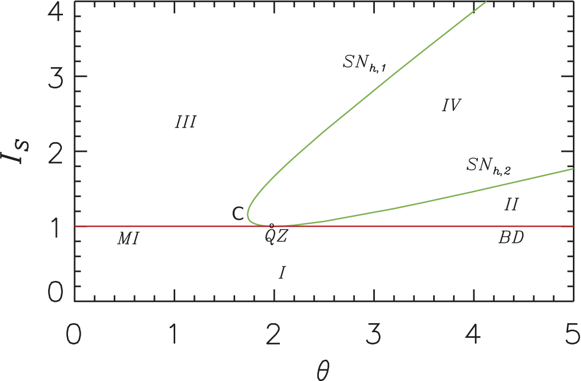
Figure 5: (Color online) All different regions that have a qualitatively different spatial eigenspectrum are shown in the parameter plane ($\theta,I_{s}$), as obtained from Eq. (6). The notation used is further clarified in Table 1.

Figure 5 shows the organization of the spatial eigenvalues corresponding to the HSSs in the parameter plane ($\theta,I_{s}$). In order to keep a closer connection to the experimental control parameters, however, we prefer plotting the structure of the spatial eigenvalues in the parameter plane ($\theta,u_{0}$), shown in Figure 6. In the plane ($\theta,u_{0}$), we only report the spatial eigenvalues corresponding to the lower branch HSS in the bistable region for $\theta>\sqrt{3}$ . In both figures, all labels are defined in Table 1, allowing to understand the different regions. Here below, we will discuss the different regions in Figure 6 in more detail.

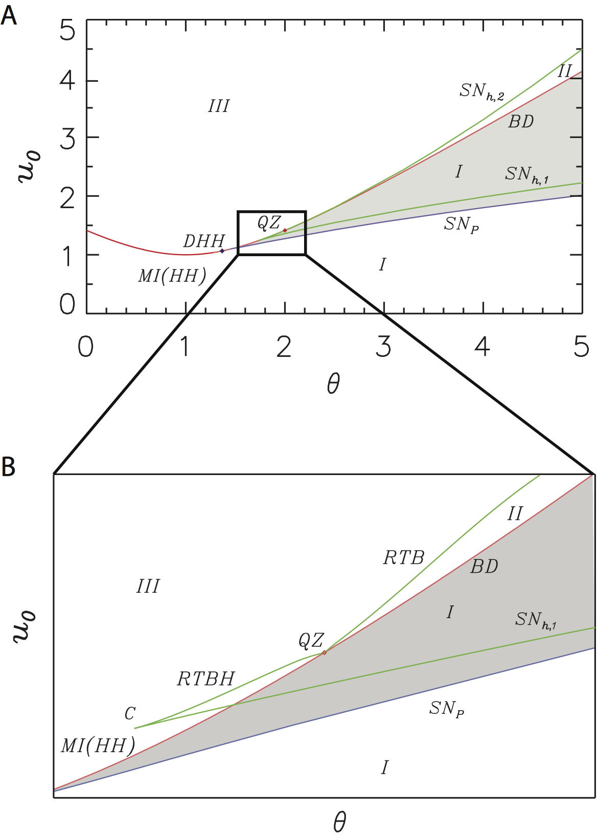
Figure 6: (Color online) In Panel A all different regions that have a qualitatively different spatial eigenspectrum are shown in the parameter plane ($\theta,u_{0}$), as obtained from Eq. (6). In the bistable region between $\mathrm{SN}_{h1}$ and $\mathrm{SN}_{h2}$, $I_{s}$ in Eq. (6) is chosen such that it corresponds to the (stable) lower intensity HSS. The notation used is further clarified in Table 1. $\mathrm{SN}_{P}$ denotes the saddle-node bifurcation where the (stable) pattern is born. The light gray region denotes the region where one can expect to find single and multiple CSs. Panel B shows a closer zoom of the organization of the spatial eigenvalues around the Quadruple Zero (QZ) point where all eigenvalues are zero.

A pair of double zeros of Eq. (6) define a MI line for $\theta<2$ in parameter space (Figure 6) given by

$$u_{0}=\sqrt{1+(1-\theta)^{2}}\ .$$ (8)

This corresponds to $I_{s}=1$ (see also Figure 5). This degenerate pair of double zeros is given by the purely imaginary eigenvalues $\lambda=\pm i\sqrt{2-\theta}$. In dynamical systems theory this bifurcation is known as a Hamiltonian-Hopf (HH). The Hamiltonian-Hopf bifurcation line separates the region I where the HSS is a double-focus (has a quartet of complex eigenvalues) from region III where the HSS is a double-center with four purely imaginary spatial eigenvalues. In this region III the HSS is unstable to spatiotemporal perturbations and patterned solutions develop.

The MI becomes a Belyakov-Devaney (BD) transition for $\theta>2$ through a Quadruple Zero (QZ) point at $\theta=2$, where $\lambda=0$ with multiplicity four. On the BD line the spatial eigenvalues are given by two pairs of pure real eigenvalues $\lambda=\pm\sqrt{\theta-2}$. Note that, as the MI (HH), the BD also occurs for $I_{s}=1$, although, strictly speaking, it is not a real bifurcation as $\text{Re}(\lambda)\neq 0$ at the transition. The BD line separates region I from region II, where the HSS is a double-saddle. After crossing this line into region II the HSS does not lose its stability and no patterned solutions develop until $\mathrm{SN}_{h,2}$ is crossed.

For $\theta>2$ the $\mathrm{SN}_{h,2}$ is a reversible Takens-Bogdanov (RTB) bifurcation with two zero spatial eigenvalues and two real eigenvalues ($\pm q_{0}$). For $\theta<2$ the $\mathrm{SN}_{h,2}$ is a reversible Takens-Bogdanov-Hopf (RTBH). On the RTBH line two eigenvalues are zero and two are purely imaginary ($\pm ik_{0})$ (see Figure 6B and Table 1).

In addition to the properties of HSSs, the spatial eigenvalues also explain the asymptotic behavior of the CS profile as $\varphi\rightarrow\pm\infty$. The present work focuses on CSs that fall in the general class of localized structures that arise through the connection of a stable homogeneous state and a subcritical pattern Pomeau (1986); Thual and Fauve (1990); Tlidi et al. (2007); Woods and Champneys (1999); Coullet et al. (2000). In the context of the spatial dynamics, such localized solutions are homoclinic orbits to a fixed point (the HSS), that pass very close (arbitrarily close increasing the number of peaks of the CS) to a periodic orbit (the patterned state), see Figure 7. The shape of the front leaving and approaching the HSS (at the same rate, due to reversibility) is given by the leading spatial eigenvalues found by solving (6). In order for (multiple) CSs to exist in any arbitrary order in the nonlinear resonator, it is required for the fronts to have oscillatory tails, so that the tails avoid the merging and annihilation of CSs Colet et al. (6801); Gelens et al. (6804). Various CSs in the system are able to coexist in the cavity as they can lock to each other via their overlapping oscillatory tails, and this has been shown to determine the possible locations (and separations) of CSs in a nonlinear cavity described by the LLE Kozyreff and Gelens (2011). Eq. (6) should exhibit a complex quartet of eigenvalues in such a case.

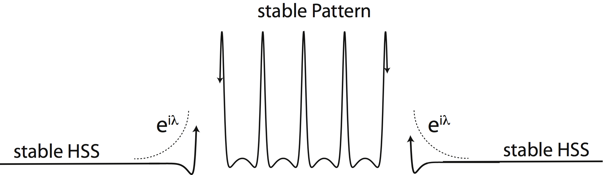
Figure 7: Sketch of the spatial dynamics leading to CSs. A CS can be interpreted as a heteroclinic connection from a stable HSS to a stable pattern and another one from the pattern back to the HSS. The trajectory approaches the HSS according the leading spatial eigenvalues $\lambda$ of the HSS, which characterize the shape of the CS tails.

The region where the stable homogeneous solution has a quartet of complex eigenvalues is Region I. The gray region in Figure 6 is the area where region I overlaps with the region of stable patterned solutions (above the $SN_{p}$ line ), such that all conditions are favorable to find CSs. Figure 8 provides more insight into how the real part $q_{0}$ and the imaginary part $k_{0}$ of the spatial eigenvalues of the stable HSS depend on the system parameters, $(\theta,u_{0})$. One can see that in the bistable region, $\theta>\sqrt{3}$, $k_{0}$ is quite small and decreases as the detuning $\theta$ increases, while the real part $q_{0}$ strongly increases for higher $\theta$. Therefore, the oscillatory tails of a CS will be strongly damped at higher values of the detuning $\theta$.

Isolated localized structures, formed by either a single peak or a number of closely packed peaks, can also exist in Region II for intracavity intensities above $I_{s}=1$, since the stable HSS still coexists with patterned solutions. In this region, however, CSs have monotonic tails and two separated CSs will move towards each other and merge.

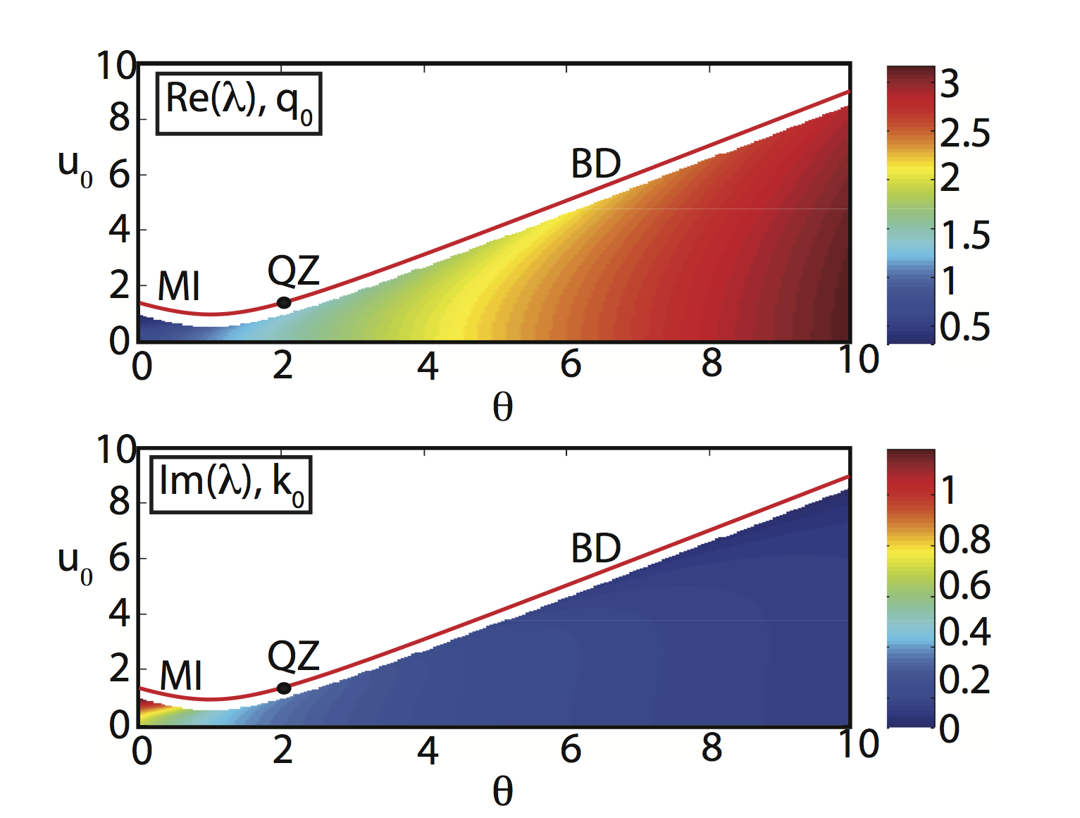
Figure 8: (Color online) In the Region I, where all spatial eigenvalues are a quartet of complex eigenvalues $\lambda_{s}=\pm q_{0}\pm ik_{0}$, we plot the real part $q_{0}$ and the imaginary part $k_{0}$ as a function of the detuning $\theta$ and the pump amplitude $u_{0}$.

V Temporal dynamics of cavity solitons

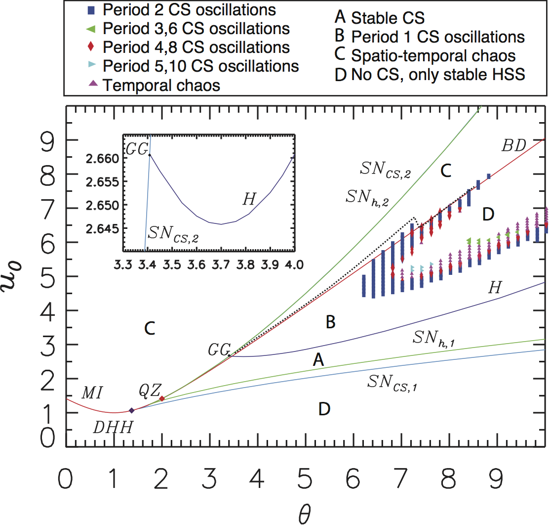
Figure 9: (Color online) The temporal dynamics of single CSs are shown and related to the transition lines obtained from the spatial dynamics also depicted in Figure 6. In region A single CSs are stable. Such CSs can be destabilized by a Hopf bifurcation $H$ leading to time-oscillating CSs, found in region B. In region C spatio-temporal chaos is found. In region D only the stable HSS is found. Finally, more complicated time dynamics such as temporal chaos is found in the region denoted by the markers. For more information about the notation of the spatial dynamics, we refer to Table 1. The inset shows a zoom of the bifurcation lines around the Gavrilov-Guckenheimer (GG) point.

In this Section, we characterize the regions of existence of single CSs in the parameter space ($u_{0},\theta$) defined by the pump power and the cavity detuning. In Figure 9, we have again plotted all characteristic lines obtained from our analysis of the spatial dynamics in the previous Section (see also Figure 6). Moreover, by combining linear stability analysis and time evolution simulations, we have characterized not only the existence of CSs, but also their temporal stability and dynamics (see also Leo et al. (2013a)). Using a Newton-Raphson method we can numerically track the CS solutions in parameter space and calculate their temporal stability. This allows to accurately determine the location of the Hopf bifurcation line $H$. All other dynamical regimes have been determined numerically using time evolution simulations. In Region A, stable CSs can be found. This region is delimited by the saddle-node bifurcation $\mathrm{SN}_{\mathrm{CS},1}$ (which largely coincides with $\mathrm{SN}_{P}$ in the bistable region) and the Hopf bifurcation line $H$ where the CS is destabilized. One can notice that the region of existence of stable CSs is largely within the gray region of Figure 6.

When crossing the Hopf bifurcation line $H$, the CS is no longer stable and displays time-periodic oscillations. This region B has recently also been demonstrated experimentally Leo et al. (2013a). An example of such a Hopf instability is shown in Figures 10 and 11. Figure 10 shows the bifurcation diagram of the single peak CS for a detuning $\theta=5$, showing the presence of a Hopf instability $H$. Crossing this Hopf bifurcation, the CS still exists and remains localized, but oscillates in time with a fixed period, see Figure 11A. The corresponding frequency comb thus also similarly oscillates in time as shown in Figure 11B. Examples of how both the CS profile and the frequency comb change during one oscillation period are given in Figure 11C-D. As the CS oscillates, the envelope of the frequency comb is modulated. Such modulation becomes more pronounced as the amplitude of the CS oscillation increases with increasing values of the pump power $u_{0}$ and detuning $\theta$. The simultaneous occurrence of a Hopf bifurcation and a saddle-node bifurcation, determined by the three temporal eigenvalues $\lambda_{a,b}=\pm i\omega$ and $\lambda_{c}=0$, with $\omega>0$, defines the codimension-$2$ point known as Gavrilov-Guckenheimer (GG) or Fold-Hopf bifurcation Guckenheimer and Holmes (1983). Thus, the Hopf bifurcation line emerges from the GG point, and although the Hopf line looks like it terminates perpendicularly to $\mathrm{SN}_{\mathrm{CS},2}$, the inset in Figure 9 shows that it in fact approaches the GG point in a tangential manner.

For higher values of the detuning more complex oscillatory behavior can be found as well, such as period-2 oscillations, period-3 oscillations, period-N oscillations and eventually temporal chaos Leo et al. (2013a). An example of such temporal chaos is given in Figure 12 where one can see that the CS remains localized, but its envelope is oscillating in a chaotic way in time. Likewise, the envelope of the corresponding frequency comb will change chaotically in time. For higher values of the pump power $u_{0}$ one also encounters large regions with a different type of chaotic response, called spatio-temporal chaos or optical turbulence, as denoted by the letter C in Figure 9. An example of such chaotic behavior is shown in Figure 13, where it is clear that one can no longer distinguish clear localized CSs. Instead the entire cavity is oscillating in a chaotic manner. The envelope of the corresponding frequency comb is no longer smooth but has significant variations of the amplitude from mode to mode due to the many different wavelengths participating in the dynamics, and it is much flatter. This regime is the one dominating the parameter space for large input powers. It can be reached directly from the HSS crossing the line $\mathrm{SN}_{h,2}$ (Figure 9) or through the instabilities of a CS for powers around the $BD$ line. The spatiotemporal chaotic regime coexists with the HSS for a range of input powers below $\mathrm{SN}_{h,2}$. The exact scenario that leads to such spatio-temporal chaos coming from a CS needs further characterization, but is seems to be closely related to the Belyakov-Devaney (BD) line where the oscillatory feature associated to the spatial eigenvalues of the HSS is lost and the tails of the CS approach the HSS in a monotonic manner. The origin of the temporal chaos observed for higher values of detuning is also currently unknown, but might originate from the unfolding of the GG point Gaspard (1993). These two points will be studied in more detail elsewhere.

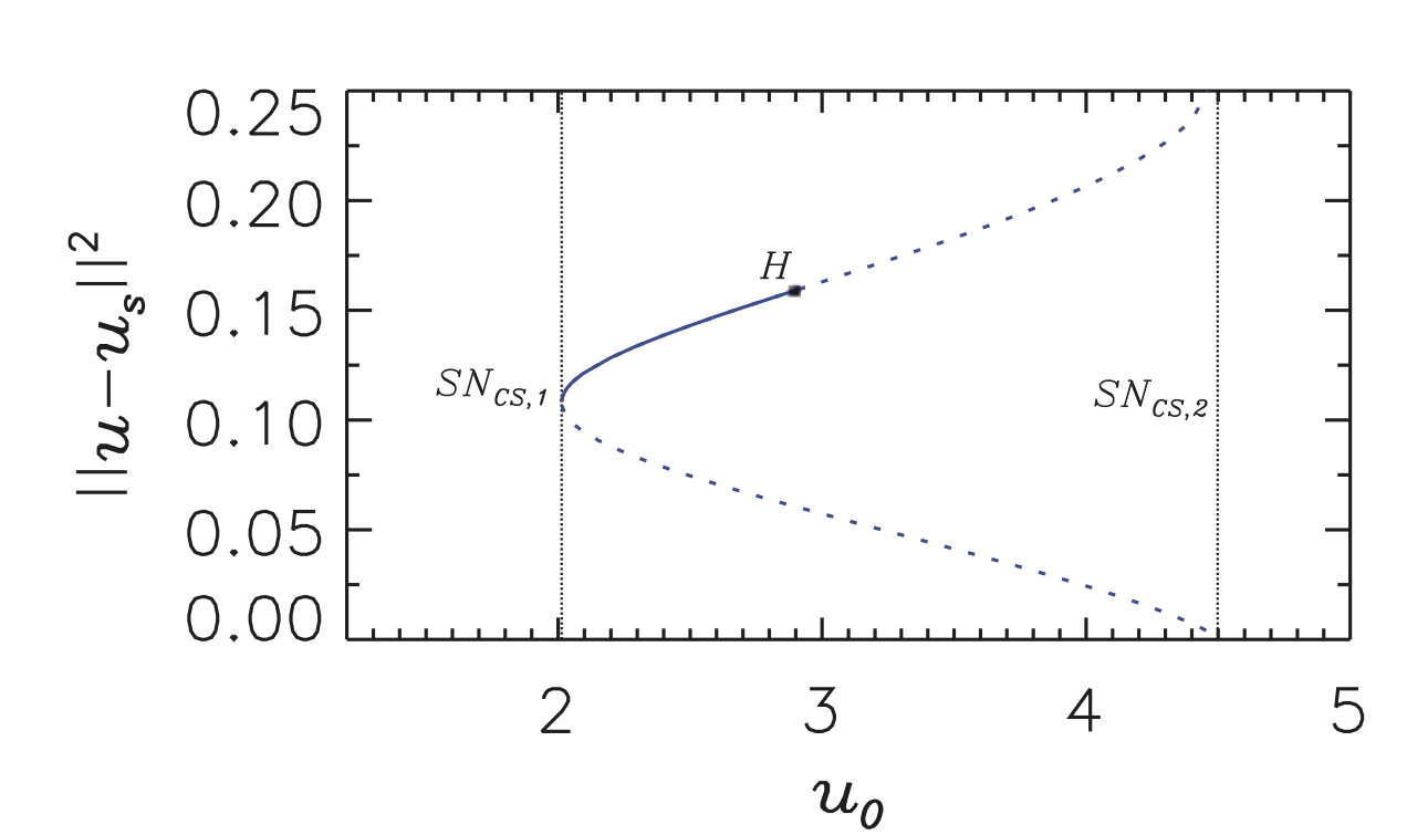
Figure 10: Bifurcation diagram of the single peak CS, showing the presence of a Hopf instability $H$ for $\theta=5$. Solid (dashed) lines represent stable (unstable) CSs.

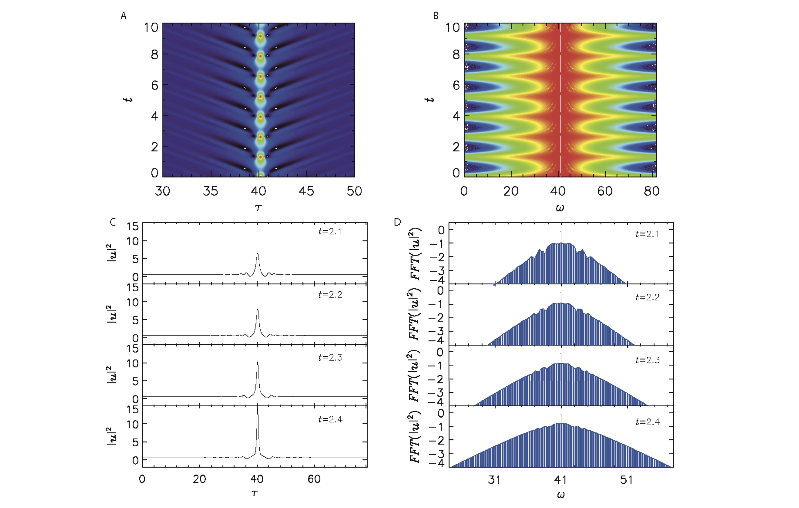
Figure 11: (Color online) Spatio-temporal evolution of a CS and its corresponding frequency comb is plotted for $u_{0}=3.5$ and $\theta=5$. Panels A and B show the time evolution in real and frequency space respectively. Panels C and D show several profiles within one oscillation period of the CS, both in the time (D) and frequency domain (E).

Figure 12: (Color online) Spatio-temporal evolution of a CS and its corresponding frequency comb is plotted for $u_{0}=6.9$ and $\theta=10$. The panels show the same as in Figure 11, but now for temporal chaos.

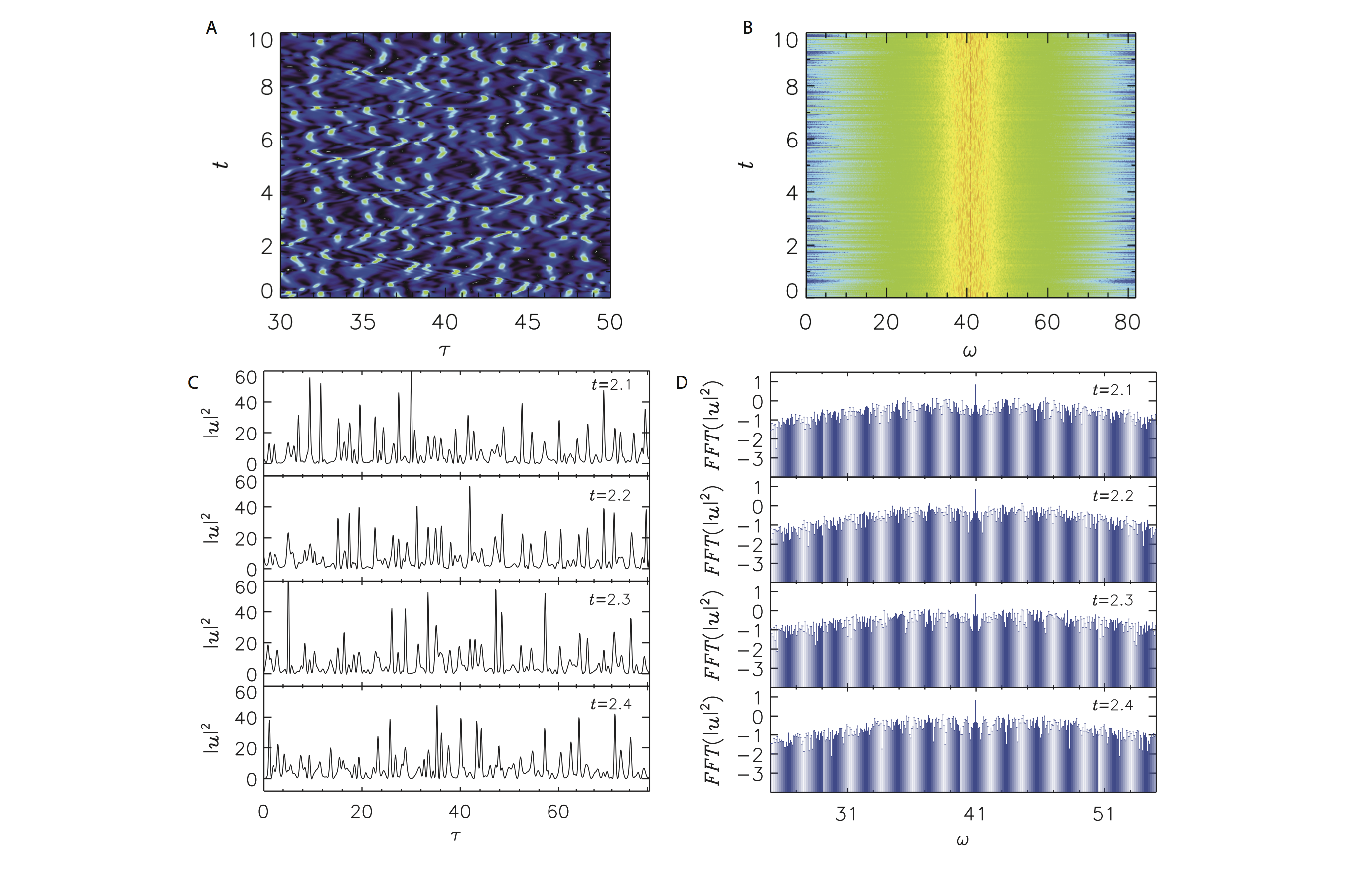
Figure 13: (Color online) Spatio-temporal evolution of a CS and its corresponding frequency comb is plotted for $u_{0}=8$ and $\theta=8$. The panels show the same as in Figure 11, but now for spatio-temporal chaos.

VI Concluding remarks

We have presented a comprehensive overview of the dynamics of the LLE with one transverse dimension in relation with the generation of frequency combs. Many different dynamical regimes, going from a single peak stationary CS to spatio-temporal chaos, are available by changing the input pump and detuning as summarized in Figure 9. On the one hand the LLE finds applications to many different nonlinear optical cavities, and on the other hand it is a prototypical model for the study of cavity solitons. Therefore many of the conclusions concerning the generation of frequency combs from the different dynamical regimes are applicable to other systems displaying CSs.

Due to the fact that many different dynamical regimes are supported in the LLE, this model offers several different possibilities for the generation of frequency combs. In particular the coexistence of multiple solutions differing only in the number of peaks circulating in the cavity offers the possibility to tune the shape of the comb without changing the parameters of the system. To target particular solutions, suitable initial conditions must be seeded in the cavity though. This observation may explain the variations in the shape of Kerr frequency combs observed in experiments with microresonators after the pump field is interrupted and restarted.

Beyond regimes of stationary CSs, in very wide parameter range the LLE displays dynamical regimes, going from regularly oscillating CSs to chaotic CSs and spatiotemporal chaos. Since these regimes appear for higher values of the input pump amplitude and the detuning, they have a much broader bandwidth. The amplitude of the Fourier modes is, however, not constant over time. Given the size of the parameter space associated with these solutions, one cannot preclude that some reported experimental spectra have actually been obtained in this regime and, owing to the slow speed of optical spectrum analyzers, are therefore averaged over the dynamics.

VII Acknowledgments

We thank P. Colet and F. Leo for stimulating discussions. This research was supported by the Research Foundation - Flanders (FWO), by the Spanish MINECO and FEDER under Grants FISICOS (FIS2007-60327) and INTENSE@COSYP (FIS2012-30634), by Comunitat Autonoma de les Illes Balears, and by the Belgian Science Policy Office (BelSPO) under Grant No. IAP 7-35. S. Coen also acknowledges the support of the Marsden Fund of the Royal Society of New Zealand.

References

- Cundiff et al. (2008) S. Cundiff, J. Ye, and J. Hall, Sci. Am. 298, 74 (2008).
- Del’Haye et al. (2007) P. Del’Haye, A. Schliesser, O. Arcizet, T. Wilken, R. Holzwarth, and T. J. Kippenberg, Nature 450, 1214 (2007).
- Kippenberg et al. (2011) T. J. Kippenberg, R. Holzwarth, and S. A. Diddams, Science 332 (2011).
- Coen et al. (2013) S. Coen, H. G. Randle, T. Sylvestre, and M. Erkintalo, Opt. Lett. 38, 37 (2013).
- Coen and Erkintalo (2013) S. Coen and M. Erkintalo, Opt. Lett. 38, 1790 (2013).
- Chembo and Menyuk (2013) Y. Chembo and C. Menyuk, Phys. Rev. A 87, 053852 (2013).
- Leo et al. (2010) F. Leo, S. Coen, P. Kockaertl, S.-P. Gorza, P. Emplit, and M. Haelterman, Nature Photon. 4, 471 (2010).
- Lugiato and Lefever (1987) L. A. Lugiato and R. Lefever, Phys. Rev. Lett. 58, 2209 (1987).
- Matsko et al. (2011) A. B. Matsko, A. A. Savchenkov, W. Liang, V. S. Ilchenko, D. Seidel, and L. Maleki, Opt. Lett. 36, 2845 (2011).
- Barland et al. (2002) S. Barland, J. R. Tredicce, M. Brambilla, L. A. Lugiato, S. Balle, M. Giudici, T. Maggipinto, L. Spinelli, G. Tissoni, T. Knödl, M. Miller, and R. Jäger, Nature 419, 699 (2002).
- McSloy et al. (2002) J. M. McSloy, W. J. Firth, G. K. Harkness, and G.-L. Oppo, Phys. Rev. E 66, 046606 (2002).
- Scroggie et al. (1994) A. J. Scroggie, W. J. Firth, G. S. McDonald, M. Tlidi, R. Lefever, and L. A. Lugiato, Chaos, Solitons and Fractals 4, 1323 (1994).
- Gomila et al. (2007) D. Gomila, A. J. Scroggie, and W. J. Firth, Physica D 227, 70 (2007).
- Firth et al. (2002) W. J. Firth, G. K. Harkness, A. Lord, J. M. McSloy, D. Gomila, and P. Colet, J. Opt. Soc. Am. B 19, 747 (2002).
- Gomila et al. (2007) D. Gomila, A. Jacobo, M. A. Matías, and P. Colet, Phys. Rev. E 75, 026217 (2007).
- McSloy et al. (1990) J. M. McSloy, W. J. Firth, G. K. Harkness, and G.-L. Oppo, J. Opt. Soc. Am. B 7, 1328 (1990).
- Herr et al. (0733) T. Herr, V. Brasch, J. D. Jost, C. Y. Wang, N. M. Kondratiev, M. L. Gorodetsky, and T. J. Kippenberg, (arXiv:1211.0733).
- Foster et al. (2011) M. A. Foster, J. S. Levy, O. Kuzucu, K. Saha, M. Lipson, and A. L. Gaeta, Opt. Express 19, 14233 (2011).
- Turaev et al. (2012) D. Turaev, A. G. Vladimirov, and S. Zelik, Phys. Rev. Lett. 108, 263906 (2012).
- Leo et al. (2013a) F. Leo, L. Gelens, P. Emplit, M. Haelterman, and S. Coen, Opt. Express 21, 9180 (2013a).
- Gelens et al. (2008) L. Gelens, D. Gomila, G. Van der Sande, J. Danckaert, P. Colet, and M. A. Matías, Phys. Rev. A 77, 033841 (2008).
- Leo et al. (2013b) F. Leo, A. Mussot, P. Kockaert, P. Emplit, M. Haelterman, and M. Taki, Phys. Rev. Lett. 110, 104103 (2013b).
- Tlidi and Gelens (2010) M. Tlidi and L. Gelens, Opt. Lett. 35, 306 (2010).
- Mitschke et al. (1996) F. Mitschke, G. Steinmeyer, and A. Schwache, Physica D 96, 251 (1996).
- Gomila and Colet (2003) D. Gomila and P. Colet, Phys. Rev. A 68, 011801 (2003).
- Champneys (1998) A. R. Champneys, Physica D 112, 158 (1998).
- Hunt et al. (2000) G. W. Hunt, M. A. Peletier, A. R. Champneys, P. D. Woods, M. A. Wadee, C. J. Budd, and G. J. Lord, Nonlinear Dynamics 21, 3 (2000).
- Knobloch and Wagenknecht (2005) J. Knobloch and T. Wagenknecht, Physica D 203, 82 (2005).
- Burke and Knobloch (2006) J. Burke and E. Knobloch, Phys. Rev. E 73, 056211 (2006).
- Kozyreff and Chapman (2006) G. Kozyreff and S. J. Chapman, Phys. Rev. Lett. 97, 044502 (2006).
- Barbay et al. (2008) S. Barbay, X. Hachair, T. Elsass, I. Sagnes, and R. Kuszelewicz, Phys. Rev. Lett. 101, 253902 (2008).
- Kozyreff and Gelens (2011) G. Kozyreff and L. Gelens, Phys. Rev. A 84, 023819 (2011).
- A. Bergeon and Mercader (2008) E. K. A. Bergeon, J. Burke and I. Mercader, Phys. Rev. E. 78, 046201 (2008).
- Haragus and Iooss (2011) M. Haragus and G. Iooss, Local Bifurcations, Center Manifolds, and Normal Forms in Infinite-Dimensional Dynamical Systems (Springer, Berlin, 2011).
- Colet et al. (6801) P. Colet, M. A. Matias, L. Gelens, and D. Gomila, (arXiv:1305.6801).
- Pomeau (1986) Y. Pomeau, Physica D 23, 3 (1986).
- Thual and Fauve (1990) O. Thual and S. Fauve, Phys. Rev. Lett. 64, 282 (1990).
- Tlidi et al. (2007) M. Tlidi, M. Taki, and T. Kolokolnikov, Chaos 17, 037101 (2007).
- Woods and Champneys (1999) P. D. Woods and A. R. Champneys, Physica D 129, 147 (1999).
- Coullet et al. (2000) P. Coullet, C. Riera, and C. Tresser, Phys. Rev. Lett. 84, 3069 (2000).
- Gelens et al. (6804) L. Gelens, M. A. Matias, D. Gomila, T. Dorissen, and P. Colet, (arXiv:1305.6804).
- Knobloch (2008) E. Knobloch, Nonlinearity 21, T45 (2008).
- Balakireva et al. (2542) I. Balakireva, A. Coillet, C. Godey, and Y. K. Chembo, (arXiv:1308.2542).
- Guckenheimer and Holmes (1983) J. Guckenheimer and P. Holmes, Nonlinear Oscillations, Dynamical Systems, and Bifurcations of Vector Fields (Springer, New York, 1983).
- Gaspard (1993) P. Gaspard, Physica D 62, 94 (1993).