Finite difference numerical method for the superlattice Boltzmann transport equation and case comparison of CPU(C) and GPU(CUDA) implementations

Abstract

We present a finite difference numerical algorithm for solving two dimensional spatially homogeneous Boltzmann transport equation which describes electron transport in a semiconductor superlattice subject to crossed time dependent electric and constant magnetic fields. The algorithm is implemented both in C language targeted to CPU and in CUDA C language targeted to commodity NVidia GPU. We compare performances and merits of one implementation versus another and discuss various software optimization techniques.

1 Introduction

Numerical solutions of Boltzmann Transport Equation (BTE) are of utmost importance in the modern physics, especially in the research areas of fluid dynamics and semi-classical description of quantum-mechanical systems. In semiconductors and their nanostructures BTE is often used to describe electron dynamics with account of scattering. BTE is often solved using Monte-Carlo method [1]. Related to it is the Lattice Boltzmann Method; it is more recent and very promising [2]. Due to its numerical stability and explicit nature, Lattice Boltzmann Method lends itself quite well to the parallel implementations on Graphical Processing Units (GPU) [3, 4, 5, 6]. Finite Difference Method (FDM) is the simplest approach to the solution of BTE. However, to attain desirable numerical stability it often requires fully implicit formulation. Recently, a number of new advanced FDMs were developed. In [7] a variant of FDM is combined with Monte-Carlo method. Fully functional solver for PMOSFET devices, which among other things can utilize FDM for solving BTE, was presented in [8]. Numerical method for spatially non-homogeneous 1D BTE in application to semiconductor superlattices was recently considered in [9].

In this work, we present a FDM method for solving two-dimensional BTE that describes a semiconductor superlattice (SL) subject to a time dependent electric field along the superlattice axis and a constant perpendicular magnetic field. Superlattices are artificial periodic structures with spatial periods not found in natural solids [10]. This relatively large period of SL results in a number of unique physical features, which are interesting not only from the viewpoint of fundamental properties of solids, but also as tools in a realization of promising applications, including the generation and detection of terahertz radiation. Good overview of SL theory and basic experiments can be found in [11, 12]. SL and the configuration of applied fields are sketched in Fig. 1. In essence this configuration is close to the standard cyclotron resonance configuration. Terahertz cyclotron resonance in SL has been observed in experiment [13]. Especially interesting is the quantity of absorption of external ac electric field. When negative it indicates a signal amplification, potentially making possible to consider use of SL as a lasing medium. Theoretically, this problem was earlier considered in the limiting case of zero temperature [14]. This work also indicated that desired signal amplification can occurs within range of parameters where electron distribution is known to be spatially homogeneous. Hence, we also considered electron probability distribution function (PDF) to vary only in the momentum space.

Our numerical scheme and software that implements it, are used to analyse electron dynamics in SL at arbitrary temperatures. It combines Crank-Nicolson [15] and Leap-Frog algorithms. Leap-Frog algorithm is a variant of symplectic integrators, which are known to preserve area in the phase space and are unconditionally stable [16, 17]. We develop several implementations of our numerical scheme. One implementation uses C programming language and is targeted for CPU. Other implementations are written in CUDA and are targeted at NVidia GPU. Compute Unified Device Architecture, also known as CUDA, is parallel computing platform and C/C++ language extension for NVidia video cards. Different CUDA implementations of our numerical method primarily highlight various differences in memory access patterns, which are the most common bottlenecks for software running on video cards. We verify correctness of the method and its implementation by comparing results of our BTE simulations with the available results in the limiting case of zero temperature [14, 18] and with a case when magnetic field is absent, for which BTE has exact analytical solution [11].

2 Physical model

Figure 1: Sketch of a superlattice under the action of time dependent electric $E(t)$ and constant magnetic B fields. The electric field is directed along the superlattice axis ($x$-axis) and the perpendicular magnetic field is aligned along $z$-axis. Electron motion is considered in $(x,y)$-plane.

Boltzmann equation governs a time evolution of the electron probability density function (PDF) $f(\mathbf{k},\mathbf{r};t)$. For our system it has the following form

$$\frac{\partial f}{\partial t}+\frac{e}{\hbar}\left(\mathbf{E}+\mathbf{v}\times\mathbf{B}\right)\frac{\partial f}{\partial\mathbf{k}} +\mathbf{v}(\mathbf{k})\frac{\partial f}{\partial\mathbf{r}}=\left(\frac{\partial f}{\partial t}\right)_{st}$$ (1)

$$\mathbf{v}(\mathbf{k})= \frac{1}{\hbar}\frac{\partial\varepsilon}{\partial\mathbf{k}}$$ (2)

where $\mathbf{k}$ is the crystal momentum, $\mathbf{v}(\mathbf{k})$ is the electron velocity and $\varepsilon(\mathbf{k})$ is the energy dispersion relation for the lowest SL miniband [11]. We make several simplifications. As mentioned in the introduction, we assume that $f$ is spatially homogeneous and put $\partial f/\partial\mathbf{r}=0$. Secondly, the collision integral $(\partial f/\partial t)_{st}$ is taken in the most simplest form $(f_{0}-f)/\tau$, where $f_{0}$ is the equilibrium distribution function and $\tau$ is the relaxation time constant. We also limit our consideration to electron transport in a single miniband, which we describe within a tight binding approximation [12]

$$\varepsilon=\frac{\hbar^{2}k^{2}_{y}}{2m}-\frac{\Delta_{1}}{2}\cos(k_{x}d)$$ (3)

where $\Delta_{1}$ is the width of the miniband, $d$ is the period of SL and $m$ is the effective electron mass along SL layers. To make this system of equations (1) (2) and (3) dimensionless we make the following substitutions.

$$\phi_{x}= k_{x}d \qquad\phi_{y}= k_{y}d/\sqrt{\alpha}$$ (4)

$$E/E_{*}\to E \qquad E_{*}= \frac{\hbar}{ed\tau}$$

$$eB\tau/\sqrt{mm_{x}}\to B \qquad t\tau\to t$$

$$\alpha= m/m_{x} \qquad m_{x}= \frac{2\hbar^{2}}{\Delta_{1}d^{2}}$$

And in view of geometry of out system BTE (1) takes form

$$\frac{\partial f}{\partial t}+\left(E+B\phi_{y}\right)\frac{\partial f}{\partial\phi_{x}}-B\sin(\phi_{x})\frac{\partial f}{\partial\phi_{y}}=f_{0}-f$$ (5)

The PDF $f(\phi_{x},\phi_{y};t)$ can formally extend indefinitely along the $y$-axis, but practically this extension is always limited by relaxation to the equilibrium distribution $f_{0}(\phi_{x},\phi_{y})$. In the variables $\phi_{x}$ and $\phi_{y}$ normalization condition for both $f(\phi_{x},\phi_{y})$ and $f_{0}(\phi_{x},\phi_{y})$ takes the following form.

$$\sqrt{\alpha}\int^{\pi}_{-\pi}\text{d}\phi_{x}\int^{+\infty}_{-\infty}\text{d}\phi_{y}f(\phi_{x},\phi_{y})=1$$ (6)

From (3) it follows that $f(\phi_{x},\phi_{y};t)$ is periodic along the $x$-axis with the period $2\pi$. Therefore, $\phi_{x}$ can be considered only within the first Brillouin zone defined from $-\pi$ to $\pi$. The periodicity allows us to represent both $f$ and $f_{0}$ as the Fourier series

$$f_{0}= \sum_{n=0}^{\infty}a^{(0)}_{n}\cos(n\phi_{x})$$ (7)

$$f=\sum_{n=0}^{\infty}a_{n} \cos(n\phi_{x})+b_{n}\sin(n\phi_{x})$$ (8)

where the Fourier coefficients $a^{(0)}_{n}$, $a_{n}$ and $b_{n}$ are functions of $\phi_{y}$ and the last two are also functions of time. In the Fourier representation, BTE (5) is transformed to the infinite set of differential equations

$$\frac{\partial a_{n}}{\partial t}=a^{(0)}_{n}- a_{n}-n(E+B\phi_{y})b_{n}+\frac{B}{2}\left(\frac{\partial b_{n+1}}{\partial\phi_{y}}-\frac{\partial b_{n-1}}{\partial\phi_{y}}\right)$$ (9)

$$\frac{\partial b_{n}}{\partial t}=-b_{n}+ n(E+B\phi_{y})a_{n}+\frac{B}{2}\left(\chi(n)\frac{\partial a_{n-1}}{\partial\phi_{y}}-\frac{\partial a_{n+1}}{\partial\phi_{y}}\right)$$ (10)

$$\chi(n)=\begin{cases}2&:n=1\\ 1&:n\neq 1\end{cases}$$ (11)

And the normalization condition (6) becomes

$$2\pi\sqrt{\alpha}\int^{+\infty}_{-\infty}a_{0}(\phi_{y},t)\text{d}\phi_{y}=1$$ (12)

Eq. (12) is later used as one of the tests of accuracy of our numerical method. The equilibrium PDF $f_{0}(\phi_{x},\phi_{y})$ is assumed to be a temperature-dependent Boltzmann distribution, which with all normalization constants takes the form

$$f_{0}=\frac{1}{2\pi I_{0}(\mu)}\sqrt{\frac{\mu}{2\pi\alpha}} \exp{\left\{\mu\cos(\phi_{x})-\frac{\mu}{2}\phi^{2}_{y}\right\}}$$ (13)

$$\mu= \frac{\Delta_{1}}{2k_{b}T}$$ (14)

Where $I_{0}(\mu)$ is modified Bessel function of zero order. We can use this specific form of $f_{0}$ to find Fourier coefficients $a^{(0)}_{n}$

$$a^{(0)}_{n}=\frac{\sigma(n)I_{n}(\mu)}{\pi I_{0}(\mu)} \sqrt{\frac{\mu}{2\pi\alpha}}\text{exp}\left\{-\frac{\mu}{2}\phi_{y}^{2}\right\}$$ (15)

$$\sigma(n)= \begin{cases}1/2&:n=0\\ 1&:n\neq 1\end{cases}$$ (16)

where $I_{n}(\mu)$ are the modified Bessel functions of order $n$.

We also assume that initially at time $t=0$ PDF is in equilibrium state $f(\phi_{x},\phi_{y};t=0)=f_{0}(\phi_{x},\phi_{y})$, i.e. $a_{n}(t=0)=a^{(0)}_{n}$ and $b_{n}(t=0)=0$. Equations (9) and (10) do not preclude time dependency of both the electric $E$ and magnetic $B$ fields. However, keeping in line with the existing research in this field [14], here we consider a magnetic field $B$ to be constant and the electric field to be sum of a constant $E_{dc}$ and monochromatic ac $E_{\omega}\cos(\omega t)$ components. Thus the total electric field acting on electrons in SL is $E=E_{dc}+E_{\omega}\cos(\omega t)$. We are most interested in the property of absorption of ac electric field, which we defined as

$$A=\left\langle\frac{2I_{0}(\mu)v_{dr}(t)}{I_{1}(\mu)}\cos(\omega t)\right\rangle_{t}$$ (17)

Where $v_{dr}(t)$ is the instantaneous electron drift velocity along the $x$-axis and $\left\langle\dots\right\rangle_{t}$ means time averaging over the period of $2\pi/\omega$. Negative absorption indicates ac field amplification, paving the way to a lasing medium. To compute absorption we have to let the system to relax to the steady state, which happens over time period of several relaxation time constants $\tau$. In our case, since time is defined in multiples of $\tau$, see (4), in all numerical experiments we let system evolve up to time $t=10$ and then compute averages, such as absorption (17). Instantaneous drift velocity along $x$-axis used in (17) is defined as miniband velocity $v_{x}$ (2) averaged over PDF

$$v_{dr}(t)= \frac{2d}{\Delta_{1}\hbar}\iint\frac{\partial\varepsilon}{\partial p_{x}}f(p_{x},p_{y};t)\text{d}p_{x}\text{d}p_{y}$$ (18)

$$= \sqrt{\alpha}\int^{\pi}_{-\pi}\text{d}\phi_{x}\int^{+\infty}_{-\infty}\text{d}\phi_{y}\sin(\phi_{x})f(\phi_{x},\phi_{y};t)$$ (19)

which in view of Fourier expansion (8) takes the form

$$v_{dr}(t)=\pi\sqrt{\alpha}\int_{-\infty}^{+\infty}b_{1}(\phi_{y};t)\text{d}\phi_{y}$$ (20)

3 Numerical algorithm

Naive application of method of finite differences to (9) and (10) leads to either unstable and/or computationally intensive numerical system. To combat this problem we are using several methods at once. First, we discretize $a_{n}$ and $b_{n}$ along time and $\phi_{y}$ axes.

$$a^{\textstyle t\leftarrow\text{time step}}_{\textstyle n,m\leftarrow\phi_{y}\text{lattice step}}$$ (21)

and $n$ is ”harmonic number”. This forms infinite two-dimensional grid. To be computable we limit it to $n\in[0,\dots,N]$ and $m\in[0,\dots,M]$, with following boundary conditions.

$$a^{t}_{n\notin[0,\dots,N],m\notin[0,\dots,M]}=0$$ (22)

$$b^{t}_{n\notin[1,\dots,N],m\notin[0,\dots,M]}=0$$ (23)

Both upper limits $N$ and $M$ have to be adjusted manually depending on strength of electric and magnetic fields and inverse temperature $\mu$, which smears distribution function $f$ in the phase space. Along the $y$-axis $\phi_{y}$ is discretized with step $\Delta\phi$ and it becomes function of lattice number $m$.

We write two forms of equations (9) and (10). One using forward differences and one using partial backward differences, i.e. on the right side of equal sign we are going to write partial derivatives at time $t$ while everything else at time $t+1$ and will follow standard procedure of Crank-Nicolson scheme by adding these two, forward and backward differences equations. First two equations (24) and (25) below are written in forward differencing scheme and last two (26) and (27) in backward differencing scheme

$$a^{t+1}_{n,m}-a^{t}_{n,m}= a^{(0)}_{n,m}\Delta t-a^{t}_{n,m}\Delta t-2b^{t}_{n,m}\mu^{t}_{n,m}+B^{t}_{n,m}$$ (24)

$$b^{t+1}_{n,m}-b^{t}_{n,m}= -b^{t}_{n,m}\Delta t+2a^{t}_{n,m}\mu^{t}_{n,m}+A^{t}_{n,m}$$ (25)

$$a^{t+1}_{n,m}-a^{t}_{n,m}= a^{(0)}_{n,m}\Delta t-a^{t+1}_{n,m}\Delta t-2b^{t+1}_{n,m}\mu^{t+1}_{n,m}+B^{t}_{n,m}$$ (26)

$$b^{t+1}_{n,m}-b^{t}_{n,m}= -b^{t+1}_{n,m}\Delta t+2a^{t+1}_{n,m}\mu^{t+1}_{n,m}+A^{t}_{n,m}$$ (27)

where

$$\beta^{t}_{m}= E^{t}+B^{t}\phi_{y}(m)$$ (28)

$$\mu^{t}_{n,m}= n\beta^{t}_{m}\Delta t/2$$ (29)

$$A^{t}_{n,m}=\frac{\alpha B\Delta t}{4\Delta\phi}(\chi(n)[a^{t}_{n-1,m+1}- a^{t}_{n-1,m-1}]-a^{t}_{n+1,m+1}+a^{t}_{n+1,m-1})$$ (30)

$$B^{t}_{n,m}=\frac{\alpha B\Delta t}{4\Delta\phi}(b^{t}_{n+1,m+1}- b^{t}_{n+1,m-1}-b^{t}_{n-1,m+1}+b^{t}_{n-1,m-1})$$ (31)

Application of Crank-Nicolson scheme [15] leads to

$$a^{t+1}_{n,m}=\frac{g^{t}_{n,m}\nu-h^{t}_{n,m}\mu^{t+1}_{n,m}}{\nu^{2}+\left(\mu^{t+1}_{n,m}\right)^{2}}$$ (32)

$$b^{t+1}_{n,m}=\frac{g^{t}_{n,m}\mu^{t+1}_{n,m}-h^{t}_{n,m}\nu}{\nu^{2}+\left(\mu^{t+1}_{n,m}\right)^{2}}$$ (33)

where

$$\nu= 1+\Delta t/2$$ (34)

$$\xi= 1-\Delta t/2$$ (35)

$$g^{t}_{n,m}=a^{t}_{n,m}\xi-b^{t}_{n,m} \mu^{t}_{n,m}+B^{t}_{n,m}+a^{(0)}_{n,m}\Delta t$$ (36)

$$h^{t}_{n,m}=b^{t}_{n,m}\xi+ a^{t}_{n,m}\mu^{t}_{n,m}+A^{t}_{n,m}$$ (37)

Equation (32, 33) can be formally written in the form

$$\mathbf{z}^{t+1}_{n,m}= \mathbf{T}(\mathbf{z}^{t}_{n,m};A^{t}_{n,m},B^{t}_{n,m})$$ (38)

$$\mathbf{z}^{t}_{n,m}= (a^{t}_{n,m},b^{t}_{n,m})$$ (39)

Where $\mathbf{T}$ is an operator that allows us to step from time step $t$ to $t+1$, separated by time interval $\Delta t$. Using this operation as is leads to only conditionally stable numerical system, because $A^{t}_{n,m}$ and $B^{t}_{n,m}$ are taken at time $t$, i.e. partially this is still simple forward difference scheme. To combat this problem we introduce two staggered grids $\{\mathbf{z}^{0},\mathbf{z}^{1},...\}$ and $\{\mathbf{z}^{1/2},\mathbf{z}^{3/2},...\}$, which we call whole and fractional one respectively. We then use leap frog method where to calculate $\mathbf{z}^{t+1}$ using (38) we use $A^{t+1/2}$ and $B^{t+1/2}$ computed on fractional grid. Similar operation is performed for a step from $t+1/2$ to $t+3/2$. Thus one step from $t$ to $t+1$ becomes two steps.

$$\mathbf{z}^{t+1}_{n,m}= \mathbf{T}(\mathbf{z}^{t}_{n,m};A^{t+1/2}_{n,m},B^{t+1/2}_{n,m})$$ (40)

$$\mathbf{z}^{t+3/2}_{n,m}= \mathbf{T}(\mathbf{z}^{t+1/2}_{n,m};A^{t+1}_{n,m},B^{t+1}_{n,m})$$ (41)

And steps alternate as seen in the following picture

This algorithm has to be started first by computing values of $\mathbf{z}^{1/2}$ using (38) with time step $\Delta t/2$.

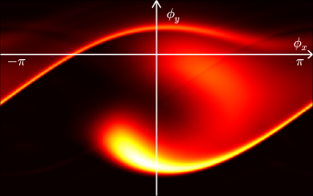
Figure 2: Example of numerical simulation showing a transient behaviour of electron probability density function (PDF) in the phase space $(\phi_{x},\phi_{y})$ at the time moment $t=1$, that is before PDF reached its stationary state. Electric and magnetic fields are applied at time $t=0$. Here the electric field is applied alone the $\phi_{x}$ axis and the magnetic field is directed perpendicularly to the plane of the plot. Initially PDF is concentrated around the center of the plot according to Boltzmann distribution function (13). Other parameters are $E_{dc}=6$ $B=4$ $E_{\omega}=0$ $\omega=0$ $\mu=3$ $\alpha=0.9496$ $dt=0.0001$

Fig. 2 represents an example of PDF computed by using our method. This heat-map like plot of PDF shows transient, i.e. before system reaches stationary state, response of the system to externally applied, at time $t=0$, electric and magnetic fields according to geometry as shown in Fig. 1.

4 Validation of correctness of numerical scheme

Complete mathematical analysis of numerical stability and correctness of numerical scheme (40) (41) is outside of the scope of this paper. However, we can compare solutions obtained by means of our numerical method with solutions obtained by other means for two limiting cases: (i) temperature approaches zero and (ii) magnetic field is absent.

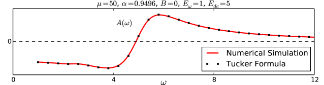
Figure 3: Absorption $A(\omega)$ for $\mu=50$ $\alpha=0.9496$ $B=0$ $E_{\omega}=1$ $E_{dc}=5$. Solid red line is computed by means of solving Boltzmann transport equation using our numerical method. Black squares are obtained by use of Tucker formula (42). Both solutions match almost perfectly.

.

If they converge then that validates our approach to solving BTE. Several test runs were performed for different values of external parameters.

When magnetic field $B$ is zero and temperature is arbitrary, analytical solution to BTE is well known and full analytical expression for absorption is known as Tucker formula [11].

$$A(\omega)=2\frac{I_{1}(\mu)}{I_{0}(\mu)}\sum^{\infty}_{n=-\infty}J_{n}(E_{\omega}/\omega) \left[J_{n+1}(E_{\omega}/\omega)+J_{n-1}(E_{\omega}/\omega)\right]\xi(E_{dc}+n\omega)$$ (42)

$$\xi(x)= x/(1+x^{2})$$ (43)

where $J_{n}(x)$ and $I_{n}(x)$ are Bessel functions of the first kind and modified Bessel functions, respectively. As an example, Fig. 3 shows results of numerical simulation (solid red line) for a given set of parameters and absorption obtained from analytical Taker formula (42), shown in black squares. You can see here that they match nearly perfectly.

The other limiting case is when temperature goes to zero ($\mu\to\infty$), in which case the equilibrium PDF $f_{0}(\phi_{x},\phi_{y})$ becomes $\delta$-function and instead of BTE (1) we can consider dynamics of a single point in the phase space $\{\phi_{x},\phi_{y}\}$. In the absence of dissipation equation (5) can be reduced to a model of single electron demonstrating pendulum dynamics [12, 14, 18].

$$\frac{\text{d}\phi_{x}}{\text{d}t}= E+B\phi_{y}$$ (44)

$$\frac{\text{d}\phi_{y}}{\text{d}t}= -B\sin(\phi_{x})$$ (45)

Which can be trivially solved numerically. Reduction of BTE to the pendulum equation is closely related to the method of characteristic curves [19, 20]. In the calculation of the drift velocity by means of (2) (3) and (44) (45) dissipation can be reintroduced through the use of exponentially decaying function of time as

$$v_{dr}(t)=\int_{-\infty}^{t}v_{x}(t)e^{-(t-t_{0})}\text{d}t_{0}$$ (46)

At low temperatures ( high values of $\mu$ ) drift velocity, and therefore absorption (17), computed by use of (19) and (46) should match. This also serves as a test of correctness of our numerical method and its implementation.

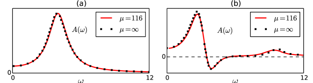
Figure 4: Absorption $A(\omega)$ for (a) dc electric field $E_{dc}=0$ (Lorentz absorption profile) and (b) $E_{dc}=6$. Other parameters are $\alpha=0.9496$, $B=4$, $E_{\omega}=0.1$. Solid red line is computed by means of solving Boltzmann transport equation using our numerical method at relatively low temperate $\mu=116$, sufficiently close to zero. Black squares are computed by solving pendulum equations (44) (45) and (46). They match very close, but not quite, due to the finite temperature.

In Fig. 4 you can see two cases of comparison of absorption. In the first case absorption is obtained by means of solving BTE using our numerical method (solid red line) at relatively low temperature corresponding to $\mu=116$ and in the second case absorption is obtained by means of solving pendulum equations (44), (45) and (46) (black squares).

When both external fields, magnetic and electric ones, are constant ($E_{\omega}=0$) then once PDF reaches stationary state we should see it reflecting characteristic features of classical pendulum. In classical pendulum separatrix divides phase space into two regions of closed and open trajectories. Indeed in Fig. 5 you can see clear correspondence between the phase portrait of classical pendulum on the left and the stationary state of PDF on the right. Notably, this correspondence and especially presence of separatrix appears at arbitrary temperature.

Finally, as mentioned before, norm of PDF at any given moment in time should be equal to one (6). Significant deviation of the norm from one can serve as an indicator of instability and/or incorrectness of numerical scheme or improper selection of compute parameters, such as too coarse or too fine (due to numerical truncation of float data type) grained mesh or time step. In all of our numerical experiments with compute times up to $t=30$, which is way beyond typical relaxation time, deviation of norm from one was less than $0.01$.

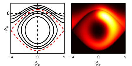
Figure 5: These two plots show correspondence between phase portrait, in ($\phi_{x}$, $\phi_{y}$) coordinates, of the classical pendulum and final stationary state of electron probability density function (PDF) for $B=4$ $E_{dc}=6.5$ $E_{\omega}=0$ $\mu=5$. Feature of separatrix, shown with dashed red line in the pendulum phase portrait (left panel) can also be seen in stationary PDF (right panel). Closed trajectories enclosed by separatrix correspond to cyclotron-like motion. Open trajectories outside of the separatrix correspond to so-called Bloch oscillations. Note that relation between proper phase portrait coordinates of classical pendulum ($\phi_{x}$, $\dot{\phi}_{x}$) and the ones used here is defined by the equation (44).

All these metrics prove that our numerical method is both, stable and gives correct solution of BTE (5).

5 CUDA and GPU computing overview

Modern GPU differ from CPU in that they have thousands ALUs at the expense of control hardware and large implicit caches of CPUs.

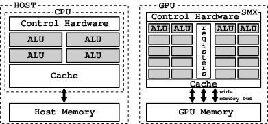
Figure 6: Simplified logical scheme of host computer and GPU that highlights differences between two. Notable is abundance of ALUs in modern day GPU, which reaches into thousands and fast wide memory bus comparing to slow memory bus on the host computer.

In NVidia video cards these ALUs are known as ”CUDA cores”. They are grouped into rows and rows into larger units with control hardware and explicit caches. These units are known as Streaming Multiprocessors (SMX). In turn a single card often contains dozen of SMX units. Abundance of ALUs makes for a need of dedicated memory and wide memory bus directly on GPU. For example in GTX680 memory bandwidth is approximately 192GB/sec., while Intel Core i7 CPU with sandy bridge architecture provides only 37GB/sec of aggregate bandwidth. In general all of the ALUs in a video card can be executed in parallel, although in actuality their execution in SMXs is scheduled in groups of 32 threads known as warps. This very large degree of parallelism commonly leads to saturation of memory bus between on-board GPU memory and SMXs, which means that while programming for GPU significant speed enhancements can be made by optimising memory access patterns and using explicitly available caches [4, 21, 22]. Misaligned and uncoalesced memory access is much slower than indicated by maximum available bandwidth. Such access patterns are common problem points in CUDA programs. Thus in general CUDA software should try to minimize writing and reading to and from memory. It is common to refer to main computer as host and installed GPU as device. Simplified logical layout of host and GPU can be seen in Fig. 6. Generally speaking GPU can be thought of as an explicitly programmable co-processor. White paper describing latest Kepler architecture of NVidia GPU can be found in [23].

CUDA is general purpose computing environment and extension to C and C++ languages developed by NVidia. It extends physical abstractions of GPU briefly described above and presents coherent API for developing general purpose software [24]. Basic introduction to CUDA programming can be found in [25] and much more comprehensive one in [26]. Software written for a GPU always consist of two parts. One part that runs on the host computer, aka host code, and another part that runs on the device, aka kernel code. It is very common in one program to have several kernels executing in sequence or in parallel, later one is possible with CUDA streams. Kernels are implicitly loaded onto the device by CUDA runtime. They can access data structures stored on both, on-board device memory and much slower, but usually much larger host memory. To be placed on the on-board device memory, data structures have to be created first on the host computer and then explicitly loaded onto the device (GPU). Execution of a kernel happens in parallel up to the capacity of the device to do so. Each parallel flow of execution is known as a thread. Threads are organized in hierarchy of grid of blocks of threads. Threads within a block can share information through very fast shared memory. Significant amount of even faster register memory also available for each thread. Number of blocks and number of threads per block have upper limits. For GTX680 GPU grids containing blocks can be three-dimensional with maximum number of blocks $65535\times 65535\times 65535$ and number of threads per blocks is limited to 1024 giving total number of threads an astonishing value of $2^{58}$. We can think of all of them as executing in parallel although in reality parallelism is ultimately limited by total number of available ALUs. At the simplest level CUDA programming could be understood as converting inner content of a loop into kernel code and replacing it with invocation of a kernel on the device. Inside of a kernel, index variable provided by a loop is replaced by a set of implicit variables indicating block number and thread number within a block. Together with dimensions of a block and grid they can be used to compute an equivalent of loop index. This is illustrated in the code snipped below, where only one of implicit variables threadIdx is shown. It defines position of thread within a block.

⬇ compute_kernel() i := threadIdx.x ... end

This kernel is later called with parameters indicating number of threads per block and number of blocks.

6 C and CUDA implementations

Using above mentioned algorithm two software packages were written . The C version that targets CPU and C/CUDA version for running on NVidia GPU. CUDA version was tested on consumer grade video card GTX680. Both implementations share the same memory layout. For C implementation memory layout is not important because computation is limited by speed of CPU. For CUDA version computation is limited by I/O speed between memory in a GPU and total number of available ALUs.

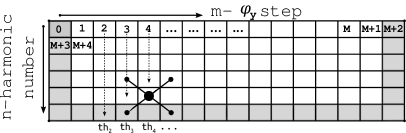
Figure 7: Row-major layout of $a_{n,m}$ and $b_{n,m}$ arrays in linear memory. Grayed out blocks correspond to boundary conditions. They have constant values of 0 and are not modified. This allows to avoid diverging data flows among groups of threads. One thread is spawned for each $m$ number, shown with dashed line. Each thread, shown as $th_{1}$, $th_{2}$ etc., is responsible for computing next values of $a$ and $b$ arrays across all $n$ harmonic numbers. Cross pattern within array shows neighbouring points that are needed to compute next value of point in the center (shown with large black circle).

Thus layout of arrays storing $a^{(0)}_{n,m}$, $a_{n,m}$ and $b_{n,m}$ and memory access patterns makes for the biggest difference in performance. We used a row-major layout shown in Fig. 7. To avoid divergent data flow at the boundaries we shift $m$ index to the right and introduce zero cells along the perimeter or each array. These zero cells, highlighted in gray in Fig. 7, ensure that boundary conditions (22) (23) are satisfied without use of if statements. Each thread computes next values of $a$ and $b$ for all of harmonic numbers for a given $m$ value. In total we define 9 two-dimensional arrays. $a^{(0)}_{n,m}$ as a0(n,m). On the whole grid $a_{n,m}$ as a_h([0,1],n,m) and $b_{n,m}$ as b_h([0,1],n,m) and on the fractional one a_f([0,1],n,m) and b_f([0,1],n,m). First index in a and b arrays can take only values of $0$ or $1$ and is used to alternate between current $t$ and next $t+1$ steps. Both CPU and GPU implementations share this logic and a time loop, which is shown below. This time loop is a part of a host code.

Time loop

⬇ cur, nxt := 0, 1 for t in [0, ..., Tmax] compute_time_step(t, cur, nxt) cur, nxt := nxt, cur end

Where compute_time_step(...) function performs movement in time from $t$ and $t+1/2$ to $t+1$ and $t+3/2$ respectively. Implementation targeted to CPU implements this function as shown in the following snippet.

CPU implementation

⬇ for m in [1,...,M+1] for n in [0,...,N) a_h(nxt, n, m) := T(a_h(cur,n,m), a_f(cur,n-1,m-1), a_f(cur,n-1,m+1), a_f(cur, n+1, m-1), a_f(cur, n+1, m+1)) b_h(nxt, n, m) := ... end end

where T(...) is implementation of operator (38). These code is repeated once more to compute $a$ and $b$ on fractional grid. There are several ways this can be transformed into a CUDA code. Two kernels are formed. One to move forward in time on the whole grid and another one for the fractional grid. Within each of the kernels several variants are possible. We identify each kernel as $K_{x}$, where $x$ is implementation number. The simplest one ($K_{1}$) is where one thread is allocated for each point of the grid. In $K_{2}$ (not shown below) we load $a$ and $b$ into __shared__ array, which is first level of explicit cache in NVidia GPU.

$K_{1}$	$K_{3}$
⬇ kernel_3(...) m := ... for n in [0,...,N) a_h(nxt, n, m) := ... b_h(nxt, n, m) := ... end end

This way we can reduce memory access since nearby threads do access the same data structures. However, they share very little data and while benefits are noticeable they are not dramatic. Better and faster code is possible. In $K_{3}$ kernel shown above, each thread is responsible for computing $a$ and $b$ for all $n$. In this implementation we do not use shared memory buffer at all. Here instruction level parallelism within loop provides very big speed improvement comparing to kernels $K_{1}$ and $K_{2}$. We can unroll loop to gain a bit more speed. In kernel $K_{4}$ loops are unrolled twice and in $K_{5}$ four times. We can also notice by looking at Fig. 7 that steps n and n+2 share $a$ and $b$ values at n+1. We take advantage of this in kernel $K_{5}$, where we split each loop into two, each steeping over n with step 2, i.e. one loop with n=[0,2,4,…] and another one with n=[1,3,5,…]. In each loop we store $a$ and $b$ values at n+1 in registers and reuse them. This provides additional speed boost without any unrolling. Due to register pressure loop unrolling in $K_{6}$ does not provide any more speed gain and may even result in program becoming slower.

7 Results

We compare time needed to perform complete time evolution of PDF $f(\phi_{x},\phi_{y};t)$ up to a given time between all of the above mentioned implementations, CPU and 6 CUDA implementations. A CPU implementation is a very simple single threaded code that does not use any of the advanced vector instructions available for modern Intel CPUs. Also OpenMP version of CPU implementation was tested. The C CPU and host code was compiled by gcc 4.6 with -O3 optimization flag. All code used float data type for storing $a_{n,m}$ and $b_{n,m}$. We found that using double data type did not affect precision nor correspondence of results with known solutions. On the other hand GTX680, being consumer grade GPU, lacks in efficient capability of performing calculations on double and its performance degrades noticeably when switching from float to double. Strait CPU implementation was single threaded and was tested on ”Intel Core i7-3770” running at 3.4GHz. CUDA implementations were tested on NVidia GTX680 with 2GB or RAM. Results of each test case are presented in Table 1. Test cases involved running each program 10 times and averaging resulted total run time. Following command line parameters were used.

⬇ bin/boltzmann_solver display=4 E_dc=7.0 PhiYmin=-6 PhiYmax=6 B=4 t-max=10 E_omega=0.1 \ omega=10 mu=116 alpha=0.9496 n-harmonics=120 dt=0.0001 g-grid=4000

Note that time step dt itself has lower limit due to numerical truncation of float data type. We found out that norm of PDF $f(\phi_{x},\phi_{y})$ starts diverging from $1$ for $\text{dt}\leq 0.00001$. Run time speed was compared against CPU implementation baseline and is presented as X times speed up. All CUDA implementations were tuned by varying block and grid sizes. Interestingly performance of kernel $K_{2}$, which uses shared memory preloaded with $a^{t}_{n,m}$ and $b^{t}_{n,m}$ values is only marginally faster then $K_{1}$. Such behaviour can be explained by the fact that values in the shared memory are reused only twice and by presence of computational flow divergence around the edges of the cached blocks. It is common to measure lattice algorithms performance in Million Lattice Updates Per Second (MLUPS). That parameter is also shown. Note that in calculation of MLUPS we count update on movement only from time $t$ to $t+1$, i.e. on the whole grid only. Otherwise, if we include updates on the fractional grid, values of MLUPS would have to be doubled. Attained peak performance is 1094 MLUPS. Faster memory bandwidth and greater number of ALUs in later GPUs such as GTX-Titan (memory bandwidth 288GB/sec; 2688 CUDA cores) should give significantly higher peak value of MLUPS. For comparison, GTX680 used for this work has memory bandwidth of 192 GB/sec and 1536 CUDA cores (ALUs).

Impl:	CPU	OpenMP	$K_{1}$	$K_{2}$	$K_{3}$	$K_{4}$	$K_{5}$	$K_{6}$
Run Time (sec):	$5216$	1537	$87.1$	$85.3$	$46.8$	$45.3$	$45.5$	$43.85$
Speed Up Times:	1	3.4	60	61	111	115	114	118
MLUPS:	9	31	551	562	1025	1059	1054	1094

Table 1: Results of testing of different implementations for a given set of parameters. Testing involved simulating evolution of electron probability density function up to a given time $t=10$ starting from initial Boltzmann distribution. CPU implementation is single threaded running on Intel i7-3770 3.4 GHz. OpenMP implementation run on the same CPU with 8 threads. The rest are CUDA versions run on GTX680. $K_{1}$ - one thread per lattice point. $K_{2}$ - same as $K_{1}$, but using shared memory. In kernel $K_{3}$ and the rest of kernels each thread computes next values for all lattice points with a given $m$-number, as seen in Fig. 7. In $K_{4}$ main loops are unrolled twice and $K_{5}$ four times. In $K_{6}$ each loop over $m$ is split in two, each steeping over 2 elements with lattice values reused in registers. Specific run times are not so important here, as they depend on the input parameters and GPU card used. Important is relative speed up time measured against baseline CPU implementation. Last row shows absolute values for MLUPS (Million Lattice Updates Per Second), which is a common measure of speed for lattice algorithms.

On the example of our Boltzmann solver code one can see that even a consumer grade video card provides significant speed boost to computational tasks amenable to parallelisation. And if we take in the account low cost of such video cards, it is now possible to perform computations on the scale which just few years ago would require access to the expensive supercomputers.

8 Conclusion

In this work we formulated a numerical method for solving two-dimensional Boltzmann transport equation applicable to the semiconductor superlattices. Its correctness and stability were verified by comparing results of simulations with results obtained by other means in two limiting cases. Several different implementations of the algorithm were presented. One written in C for CPU and several for NVidia GPU using CUDA. We show that even in the most ”naive” conversion of C to CUDA 60 fold speed improvement is attained. Trying different optimization techniques discussed in this work CUDA code attains 118 fold speed up over the single threaded C code.

9 Acknowledgement

Author expresses his gratitude to Kirill Alekseev and Jukka Isohätälä for very useful discussions on the subject of this paper and to Timo Hyart for providing some data from his dissertation for comparison with our BTE calculations.

References

- [1] L. Pareschi, G. Russo, An introduction to monte carlo method for the boltzmann equation, ESAIM: Proceedings 35 (10).
-
[2]
D. Raabe, Overview of the
lattice boltzmann method for nano- and microscale fluid dynamics in materials
science and engineering, Modelling and Simulation in Materials Science and
Engineering 12 (6) (2004) R13.
URL http://stacks.iop.org/0965-0393/12/i=6/a=R01 -
[3]
J. Tölke, Implementation of
a lattice boltzmann kernel using the compute unified device architecture
developed by nvidia, Computing and Visualization in Science 13 (1) (2010)
29–39.
doi:10.1007/s00791-008-0120-2.
URL http://dx.doi.org/10.1007/s00791-008-0120-2 - [4] M. Mawson, A. Revell, Memory transfer optimization for a lattice boltzmann solver on kepler architecture nvidia gpus, CoRR abs/1309.1983.
- [5] M. Januszewski, M. Kostur, Sailfish: a flexible multi-GPU implementation of the lattice Boltzmann method, ArXiv e-printsarXiv:1311.2404.
-
[6]
Y. Kloss, P. Shuvalov, F. Tcheremissine,
Solving boltzmann equation on {GPU}, Procedia Computer Science 1 (1) (2010)
1083 – 1091, ¡ce:title¿ICCS 2010¡/ce:title¿.
doi:http://dx.doi.org/10.1016/j.procs.2010.04.120.
URL http://www.sciencedirect.com/science/article/pii/S18770%50910001213 - [7] A. Frezzotti, G. P. Ghiroldi, L. Gibelli, Solving the Boltzmann equation on GPUs, Computer Physics Communications 182 (2011) 2445–2453. arXiv:1005.5405, doi:10.1016/j.cpc.2011.07.002.
-
[8]
A.-T. Pham, C. Jungemann, B. Meinerzhagen,
On the numerical aspects
of deterministic multisubband device simulations for strained double gate
pmosfets, Journal of Computational Electronics 8 (3-4) (2009) 242–266.
doi:10.1007/s10825-009-0301-3.
URL http://dx.doi.org/10.1007/s10825-009-0301-3 -
[9]
M. Álvaro, M. Carretero, L. Bonilla,
Numerical method for hydrodynamic modulation equations describing bloch
oscillations in semiconductor superlattices, Journal of Computational
Physics 231 (13) (2012) 4499 – 4514.
doi:http://dx.doi.org/10.1016/j.jcp.2012.02.024.
URL http://www.sciencedirect.com/science/article/pii/S00219%99112001337 -
[10]
L. Esaki, R. Tsu, Superlattice and
negative differential conductivity in semiconductors, IBM J. Res. Dev.
14 (1) (1970) 61–65.
doi:10.1147/rd.141.0061.
URL http://dx.doi.org/10.1147/rd.141.0061 - [11] A. Wacker, Semiconductor superlattices: A model system for nonlinear transport, Phys. Rep. 357 (2002) 1.
-
[12]
F. Bass, A. Tetervov,
High-frequency phenomena in semiconductor superlattices, Physics Reports 140 (5)
(1986) 237 – 322.
doi:http://dx.doi.org/10.1016/0370-1573(86)90083-9.
URL http://www.sciencedirect.com/science/article/pii/037015%7386900839 -
[13]
T. Duffield, R. Bhat, M. Koza, F. DeRosa, D. M. Hwang, P. Grabbe, S. J. Allen,
Electron mass
tunneling along the growth direction of (al,ga) as/gaas semiconductor
superlattices, Phys. Rev. Lett. 56 (1986) 2724–2727.
doi:10.1103/PhysRevLett.56.2724.
URL http://link.aps.org/doi/10.1103/PhysRevLett.56.2724 -
[14]
T. Hyart, J. Mattas, K. N. Alekseev,
Model of the
influence of an external magnetic field on the gain of terahertz radiation
from semiconductor superlattices, Phys. Rev. Lett. 103 (2009) 117401.
doi:10.1103/PhysRevLett.103.117401.
URL http://link.aps.org/doi/10.1103/PhysRevLett.103.117401 -
[15]
J. Crank, P. Nicolson, A practical
method for numerical evaluation of solutions of partial differential
equations of the heat-conduction type, Advances in Computational Mathematics
6 (1) (1996) 207–226.
doi:10.1007/BF02127704.
URL http://dx.doi.org/10.1007/BF02127704 -
[16]
E. Forest, Geometric
integration for particle accelerators, Journal of Physics A: Mathematical
and General 39 (19) (2006) 5321.
URL http://stacks.iop.org/0305-4470/39/i=19/a=S03 -
[17]
H. Yoshida, Recent progress in the
theory and application of symplectic integrators, Celestial Mechanics and
Dynamical Astronomy 56 (1-2) (1993) 27–43.
doi:10.1007/BF00699717.
URL http://dx.doi.org/10.1007/BF00699717 - [18] T. Hyart, Tunable superlattice amplifiers based on dynamics of miniband electrons in electric and magnetic fields.
-
[19]
F. Brosens, W. Magnus, Carrier
transport in nanodevices: revisiting the boltzmann and wigner distribution
functions, physica status solidi (b) 246 (7) (2009) 1656–1661.
doi:10.1002/pssb.200844424.
URL http://dx.doi.org/10.1002/pssb.200844424 -
[20]
W. Magnus, F. Brosens, B. Sorée,
Time dependent
transport in 1d micro- and nanostructures: Solving the boltzmann and
wigner–boltzmann equations, Journal of Physics: Conference Series 193 (1)
(2009) 012004.
URL http://stacks.iop.org/1742-6596/193/i=1/a=012004 -
[21]
S. Ryoo, C. I. Rodrigues, S. S. Baghsorkhi, S. S. Stone, D. B. Kirk, W.-m. W.
Hwu, Optimization
principles and application performance evaluation of a multithreaded gpu
using cuda, in: Proceedings of the 13th ACM SIGPLAN Symposium on Principles
and Practice of Parallel Programming, PPoPP ’08, ACM, New York, NY, USA,
2008, pp. 73–82.
doi:10.1145/1345206.1345220.
URL http://doi.acm.org/10.1145/1345206.1345220 - [22] S. Ryoo, C. I. Rodrigues, S. S. Baghsorkhi, S. S. Stone, D. B. Kirk, W.-m. W. Hwu, Optimization principles and application performance evaluation of a multithreaded gpu using cuda, in: Proceedings of the 13th ACM SIGPLAN Symposium on Principles and practice of parallel programming, ACM, 2008, pp. 73–82.
-
[23]
NVidia,
Nvidia’s next generation cuda compute architecture:
Kepler gk110 (2012).
URL http://www.nvidia.com/content/PDF/kepler/NVIDIA-Kepler-%GK110-Architecture-Whitepaper.pdf -
[24]
NVidia, Cuda c
programming guide (2013).
URL http://docs.nvidia.com/cuda/cuda-c-programming-guide - [25] J. Sanders, E. Kandrot, CUDA by Example: An Introduction to General-Purpose GPU Programming, 1st Edition, Addison-Wesley Professional, 2010.
- [26] N. Wilt, The CUDA Handbook: A Comprehensive Guide to GPU Programming, Pearson Education, 2013.