Band gaps in incommensurable graphene on hexagonal boron nitride

Abstract

Devising ways of opening a band gap in graphene to make charge-carrier masses finite is essential for many applications. Recent experiments with graphene on hexagonal boron nitride ($h$-BN) offer tantalizing hints that the weak interaction with the substrate is sufficient to open a gap, in contradiction of earlier findings. Using many-body perturbation theory, we find that the small observed gap is what remains after a much larger underlying quasiparticle gap is suppressed by incommensurability. The sensitivity of this suppression to a small modulation of the distance separating graphene from the substrate suggests ways of exposing the larger underlying gap.

Introduction.

The constant velocity of the charge carriers in graphene that results from the linear dispersion of the energy bands about the Dirac point gives rise to many of its intriguing properties Geim and Novoselov (2007); Geim (2009); Castro Neto et al. (2009) but also poses a serious limitation to its application in high-performance electronic devices Novoselov et al. (2012); Schwierz (2013). For logic applications, transistors with on-off ratios of order $10^{6}$ are needed, requiring band gaps of $\sim 0.4$ eV Schwierz (2013). Different approaches have been adopted to open a gap, the most promising of which is to use the interaction of graphene with a substrate to modify the linear dispersion of the bands.

The current front runners to open a band gap using a sublattice symmetry-breaking interaction are SiC Mattausch and Pankratov (2007); *Varchon:prl07; *Zhou:natm07 and hexagonal boron nitride ($h$-BN) substrates Giovannetti et al. (2007); Dean et al. (2010). Because of its flatness, similarity to graphene, and the development of practical methods for preparing single layers of graphene on hexagonal boron nitride substrates Dean et al. (2010) there has been an explosion in the number of studies of this system. $h$-BN is a very suitable insulating substrate for making graphene-based devices Britnell et al. (2012a) because it has dielectric characteristics similar to those of SiO₂, but contains fewer charged impurities and is atomically flat Lee et al. (2011); Britnell et al. (2012b). These properties result in a higher charge carrier mobility for graphene on $h$-BN compared to graphene on SiO₂ Dean et al. (2010), and in electron-hole puddles Martin et al. (2008) that are larger in size and less deep Xue et al. (2011); Decker et al. (2011).

In this paper we will show that the recently observed gap of order 30 meV Hunt et al. (2013) results from a large many-body enhanced quasiparticle gap being canceled by the incommensurability of graphene and $h$-BN that is only partially restored by a lateral variation of the height of graphene above the $h$-BN substrate. The large size of the underlying band gap and the mechanism of its cancellation suggest ways of recovering the large bare bandgap.

Graphene on top of $h$-BN experiences a perturbing potential comprising two components. First, the 1.8% lattice mismatch between the two honeycomb lattices and orientational misalignment give rise to a slowly varying component that has been observed as moiré patterns in scanning tunneling microscopy images Xue et al. (2011); Decker et al. (2011). Because of the chiral nature of the states close to the Dirac point Ando and Nakanishi (1998); *Ando:jpsj98b, this component does not open a gap Park et al. (2008a); Barbier et al. (2008); Park et al. (2008b); Burset et al. (2011); the superlattice Dirac points predicted by these effective Hamiltonian theoretical studies have recently been observed in scanning tunneling spectroscopy experiments Yankowitz et al. (2012).

Second, the heteropolar $h$-BN substrate also gives rise to a sublattice symmetry-breaking potential that opens a gap at the Dirac point when graphene and $h$-BN are commensurable Giovannetti et al. (2007). The initial failure Dean et al. (2010); Xue et al. (2011); Decker et al. (2011) to observe the band gap of order 50 meV predicted by these first principles calculations was attributed to the lattice mismatch Xue et al. (2011); Sachs et al. (2011). On the basis of binding energies calculated from first principles, it was argued that the energy gained by graphene bonding commensurably to $h$-BN was insufficient to offset the energy cost of achieving this by stretching graphene (or compressing $h$-BN). Tight-binding (TB) analyses led Xue Xue et al. (2011) and Sachs Sachs et al. (2011) to argue that the symmetry-breaking interaction between graphene and $h$-BN would average out in the incommensurable case to a much smaller (but not vanishing Kindermann et al. (2012)) band gap.

Recent temperature-dependent transport studies indicating the occurrence of a metal-to-insulator transition at the charge neutrality point at low temperatures, suggest that the situation may be more complex Ponomarenko et al. (2011); Amet et al. (2013); Hunt et al. (2013). The low temperature insulating state has been interpreted to be induced by disorder (Anderson transition) Ponomarenko et al. (2011) or to result from substrate-induced valley symmetry breaking Amet et al. (2013); Hunt et al. (2013). It has also been suggested that even small symmetry-breaking-induced band gaps may be greatly enhanced by many-body interactions Song et al. (2013).

Because the gap suppression by lattice mismatch depends on details of the approximations made in deriving effective Hamiltonians for graphene Kindermann et al. (2012), we use first-principles calculations to derive explicit $\pi$-orbital nonorthogonal TB Hamiltonians for graphene on $h$-BN that do not appeal to perturbation theory to fold the graphene-substrate interaction into an effective Hamiltonian. The band gap induced by a commensurable $h$-BN substrate survives the small lattice mismatch between graphene and $h$-BN but is indeed greatly reduced; it does not survive misaligning the two lattices. Taking into account a local variation of the graphene-$h$-BN separation and uqasiparticle energies calculated within the GW approximation of many body perturbation theory leads to a band gap of 32 meV.

Computational details.

We use density functional theory (DFT) at the level of the local density approximation (LDA) Perdew and Zunger (1981) within the framework of the plane-wave projector augmented wave (PAW) method Blöchl (1994), as implemented in VASP Kresse and Hafner (1993); Kresse and Furthmüller (1996); Kresse and Joubert (1999), to determine the electronic structure of a graphene sheet on top of a $h$-BN substrate. A plane wave basis with a cutoff energy of 400 eV is used in combination with a $36\times 36$ $k$-point grid (in a $1\times 1$ unit cell). Many-body effects are studied within the GW approximation Hedin (1965) starting with LDA Kohn-Sham (KS) orbitals Hybertsen and Louie (1986) calculated for a cell containing two $h$-BN layers and a graphene layer. We use the $GW$ implementation in VASP Shishkin and Kresse (2006), with 12 occupied and 52 empty bands and 50 points on the frequency grid. Interactions between periodic images in the $z$ direction lead to a dependence of the $GW$ band gap on the cell size that we remove by linearly extrapolating the calculated gaps as a function of the inverse cell size to infinite separation Berseneva et al. (2013).

Density functional calculations.

We start by analyzing the electronic structures of rotationally aligned, commensurable graphene$|h$-BN at the DFT and $GW$ levels, before using the results to construct a TB Hamiltonian for rotated, incommensurable structures. We focus for convenience on the three high symmetry configurations: (a) with one carbon over B, the other over N; (b) with one carbon over N, the other centered above a $h$-BN hexagon; and (c) with one carbon over B, the other centered above a $h$-BN hexagon Giovannetti et al. (2007). Panels (a)-(c) of Fig. 1 show the LDA energy bands for graphene on $h$-BN for the (a), (b) and (c) configurations at their RPA equilibrium separations of $d_{\rm eq}=$ 3.55, 3.50 and 3.35 Å Sachs et al. (2011), respectively, with LDA gaps $\Delta\varepsilon\equiv\varepsilon_{3}(K)-\varepsilon_{2}(K)$ of 30-40 meV opened at the $K$ point by the symmetry-breaking interaction with the substrate Giovannetti et al. (2007). The Dirac point is situated asymmetrically in the $h$-BN band gap about a third of the way from the top of the valence band. Apart from the formation of the small gap, the dispersion of the $\pi$ bands is largely unchanged by the interaction with the $h$-BN substrate within about 1 eV of the Dirac point.

If we expand the energy scale about the Dirac point, we see that the centers of the gaps, $[\varepsilon_{2}({\rm K})+\varepsilon_{3}({\rm K})]/2$, do not coincide for the different configurations (lower panels); the interaction between graphene and $h$-BN gives rise to an interface potential step $\Delta V$. The source of this potential step is a configuration-dependent interface dipole layer that can be visualized in terms of the electronic displacement $\Delta n({\bf r})$ obtained by subtracting the electron densities of the isolated constituent materials, $n_{\rm Gr}$ and $n_{\rm BN}$, from that of the entire system $n_{\rm Gr|BN}$ Bokdam et al. (2011); *Bokdam:prb13. The potential step is related to the dipole layer, illustrated in Fig. 1 for the (a), (b) and (c) configurations, by $\Delta V=-e^{2}/(A\epsilon_{0})\int z\Delta n({\bf r})\,dx\,dy\,dz$ where $A$ is the area of the surface unit cell and the integration is over all space.

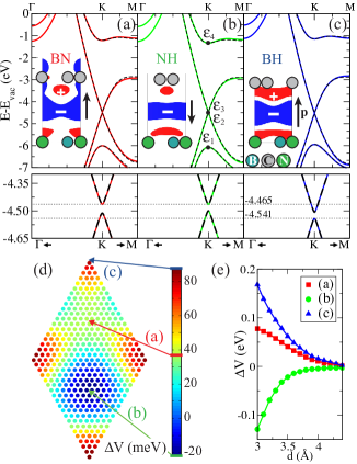
Figure 1: (Color) LDA band structures of graphene on $h$-BN for the (a), (b), and (c) commensurable structures, with respect to a common vacuum level. Solid and dashed lines give the DFT results and the TB fits, respectively. The region around the Dirac point is enlarged in the panels below. The formation of an interface dipole is illustrated by the charge displacement $-e\Delta n$ in the $yz$ plane containing B, C and N atoms. Blue and red indicate regions of negative and positive charge density, respectively, giving a dipole moment p. (d) The interface potential step $\Delta V$ as a function of the position $(x,y)$ of graphene with respect to $h$-BN, at the RPA equilibrium separation $d_{\mathrm{eq}}(x,y)$ [see Fig. 3a]. (e) Dependence of $\Delta V$ on $d$ for configurations (a)-(c).

The potential step depends sensitively on how the graphene and $h$-BN lattices are positioned. Starting from the (c) configuration, and displacing graphene laterally by $(x,y)$ yields the potential landscape $\Delta V(x,y)$ shown in Fig. 1(d). For each value of $(x,y)$, the graphene sheet is a distance $d_{\mathrm{eq}}(x,y)$, the RPA equilibrium separation, from the $h$-BN substrate. $\Delta V$ reaches appreciable values ranging from $-20$ to $90$ meV, where the minimum and maximum values are found for the high symmetry configurations (b) and (c), respectively. The full $d$-dependence of $\Delta V$ is shown for the three configurations in Fig. 1(e).

GW correction

We perform $G_{0}W_{0}$ calculations for the three symmetric configurations in order to find the many body corrections to the LDA band gaps. Figure 2 shows the quasiparticle gaps as a function of the inverse cell size $1/a$ in the direction perpendicular to the graphene sheet fn: for the three symmetric configurations and for values of the height of graphene above the $h$-BN substrate that span the full range of RPA equilibrium separations. We are interested in the band gap for an isolated layer of graphene on $h$-BN that we determine by extrapolation to $a\rightarrow\infty$. The gap is seen to increase dramatically, from 43, 28, and 30 meV (horizontal lines) in the LDA to 278, 178 and 193 meV, for the (a), (b) and (c) configurations at the RPA equilibrium separations (thick lines), respectively.

Band gap in graphene on $h$-BN

Before we use the results of the full $abinitio$ calculations for the commensurable systems to construct a TB Hamiltonian for the incommensurable case, it is useful to estimate the size of the band gaps we expect to find. We can make use of the weakness of the interaction between the graphene and $h$-BN and the large separation in energy between the Dirac point eigenvalues and the $h$-BN valence and conduction band edges to construct an effective Hamiltonian for the graphene layer by Löwdin downfolding, otherwise know as the Schur complement. The substrate can then be replaced by three effective potentials Kindermann et al. (2012): one that locally shifts the Dirac point, another that opens a local gap, and a third that has the form of a pseudo-magnetic field. By applying first order degenerate perturbation theory to the downfolded Hamiltonian, we estimate the gap of the incommensurable system to be

$$\overline{\Delta\varepsilon}=\left|\Delta\varepsilon_{\rm(b)}+\Delta\varepsilon_{\rm(c)}-\Delta\varepsilon_{\rm(a)}\right|/3,$$ (1)

in terms of the gaps of the commensurable systems.

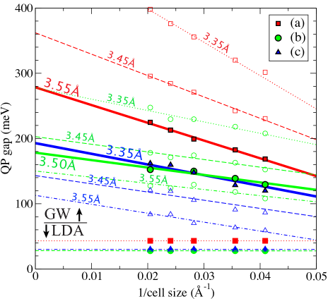
Figure 2: (Color) Quasiparticle (QP) and LDA gaps opened at the Dirac point as a function of the inverse cell size. The thick solid lines correspond to graphene at the RPA equilibrium distances of configurations (a), (b) and (c) Sachs et al. (2011). The dotted, dashed and dashed/dotted lines correspond to graphene$-h$-BN separations of 3.35, 3.45, and 3.55 Å, respectively.

This estimate should be valid in the limit that the mismatch is very small and all possible configurations are sampled equally. Using Eq. (1) and assuming that the structure is locally at its RPA equilibrium separation, we expect the band gap of aligned, incommensurable graphene on $h$-BN to be $31$ meV at the $G_{0}W_{0}$ level, as compared to 5 meV at the LDA level. Assuming the graphene sheet is flat results in much smaller $G_{0}W_{0}$ gaps of 10, 5 and 4 meV for separations of 3.35, 3.45, and 3.55 Å, respectively. This indicates that it is important to take the modulation of the equilibrium separation into account. We will find that the gaps estimated using Eq. (1) are very close to the results obtained by full numerical diagonalization of the TB Hamiltonian.

Tight-binding Hamiltonian.

The diagonal blocks of the TB Hamiltonian and overlap matrices

$$H=\left(\begin{array}[]{cc}H_{\rm Gr}&H_{\rm int}\\ H_{\rm int}^{\dagger}&H_{\rm BN}\\ \end{array}\right)\;;\;O=\left(\begin{array}[]{cc}O_{\rm Gr}&O_{\rm int}\\ O_{\rm int}^{\dagger}&O_{\rm BN}\\ \end{array}\right)$$ (2)

are first determined separately for monolayers of graphene and $h$-BN. Because isolated monolayers have reflection symmetry, the $p_{z}$ blocks of the corresponding matrices are decoupled from the $\{s,p_{x},p_{y}\}$ blocks. By introducing an overlap matrix, $H$ and $O$ can be chosen to have short range and the $abinitio$ (LDA and $GW$) bands can be fit essentially exactly. When we consider the interaction between graphene and $h$-BN, we include the interface potential step $\Delta V$ as an additional diagonal term.

We determine $\Delta V$ for incommensurable structures by interpolation and approximate incommensurable lattices by periodic superstructures. For example, the factor $1.018$ between the $h$-BN and the graphene lattice parameters can be represented by the rational approximant $56/55$, which leads to a supercell of $56\times 56\times 2$ carbon atoms and $55\times 55$ each of boron and nitrogen atoms. As the lattice mismatch is small, we assume that the graphene sheet locally follows the RPA equilibrium separation $d_{\mathrm{eq}}(x,y)$ as a function of position $(x,y)$ within this supercell, as shown in Fig. 3(a). The difference between the commensurable and incommensurable structure is schematically illustrated in Figs. 3(c) and 3(d). The potential step $\Delta V(x,y)$ can then be obtained from Fig. 1(d).

To define $\Delta V$ when the graphene lattice is rotated through an angle $\phi$ with respect to the $h$-BN substrate, we make use of the fact that $\Delta V(x,y)$ has threefold rotation symmetry and interpolate for intermediate angles. This approximation was checked for commensurable lattices where explicit DFT calculations can be performed for specific rotation angles for which the unit cell sizes are manageable.

TB: Commensurable lattices.

The remaining parameters of the TB Hamiltonian are obtained from fits to either the LDA or the GW band structures of commensurable graphene$|h$-BN structures. The band structures calculated with the TB Hamiltonian are compared to the LDA results in Figs. 1(a)-(c) (dashed lines). The TB Hamiltonian clearly yields a satisfactory fit for the three configurations shown. It also accurately captures the shift of the Dirac cone as a function of an $xy$ translation of the graphene sheet over the $h$-BN substrate. Figure 3(b) shows the position of the Dirac point (the center of the gap) with respect to the center of the $h$-BN band gap,

$$\varepsilon_{\rm D}(x,y)=\left\{[\varepsilon_{3}({\rm K})+\varepsilon_{2}({\rm K})]-[\varepsilon_{4}({\rm K})+\varepsilon_{1}({\rm K})]\right\}/2,$$ (3)

for the height profile shown in Fig. 3(a); it fits the LDA results exactly. Comparison of the LDA energy bands for a structure with graphene rotated through $21.78^{\circ}$ with respect to $h$-BN (resulting in a $\sqrt{7}\times\sqrt{7}$ unit cell with 14 carbon, 7 boron and 7 nitrogen atoms) again shows very good agreement. Because the rotated system was not used in fitting the TB Hamiltonian, the good description of the bands close to the Dirac points is an important measure of its predictive capability.

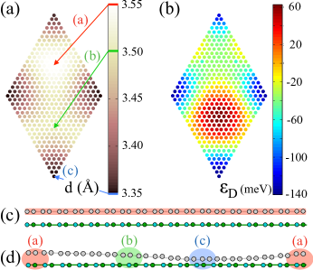
Figure 3: (Color) (a) The RPA equilibrium separation as a function of the lateral displacement of the two lattices for commensurable graphene on $h$-BN. (b) The position of the Dirac point with respect to the center of the $h$-BN band gap, $\varepsilon_{\rm D}$. The plotted values are relative to the constant $\varepsilon_{\rm D}$ obtained for graphene and $h$-BN at an infinite interlayer distance. Schematic representations of (c) commensurable and (d) incommensurable configurations of graphene on $h$-BN where the bonding locally resembles commensurable configurations.

TB: Incommensurable lattices.

It has been argued that the bonding between graphene and a $h$-BN substrate is so weak and those honeycomb structures so stiff that the small 1.8% lattice mismatch will persist in graphene$|h$-BN structures Sachs et al. (2011). For perfect alignment, i.e., $\phi=0$, this implies that even if we start at a position where the local bonding corresponds to the lowest energy [the (c) bonding configuration], the lattice mismatch will result in dephasing of the two lattices. However, the mismatch is sufficiently small that locally the hopping is indistinguishable from a commensurable system displaced by some amount $(x,y)$, with an equilibrium distance $d_{\mathrm{eq}}(x,y)$, so the Hamiltonian for the incommensurable system can be assembled with the parametrization described above. Choosing the vacuum potential as the common potential zero leads to diagonal elements of the TB Hamiltonian that depend on the local interface potential $\Delta V(x,y)$. The $h$-BN conduction and valence band edges then undulate in real space, a prediction that could be confirmed by experiment.

When $\phi=0$ and assuming that the graphene sheet follows the height profile of Fig. 3(a), we calculate a ($GW$) band gap of 32 meV. This is consistent with reports of the charge neutrality point resistance increasing with decreasing temperature Ponomarenko et al. (2011); Amet et al. (2013) and of gaps between 16 and 28 meV that were extracted from temperature dependent resistivity measurements Hunt et al. (2013). The height variation in the structure turns out to be important; using a flat graphene sheet at separations of 3.35, 3.45, and 3.55 Å, results in gaps of 10, 6, and 5 meV, respectively. This suggests that it may be possible to realize larger gaps in graphene by suitably modulating the graphene-$h$-BN spacing. For rotation angles $\phi>0^{\circ}$, the gap rapidly becomes smaller. Calculations for a $\phi=6^{\circ}$, $\delta=2.0$% incommensurable structure result in a vanishing gap. Further studies on even larger supercells corresponding to smaller angles have to be done to determine the critical angle at which a band gap is opened.

Conclusions.

Many-body calculations for commensurable graphene on $h$-BN show that quasiparticle band gaps are much larger than previously thought. Incommensurability results in a near complete cancellation of these gaps, but a detailed analysis suggests that it may be possible to realize gaps much larger than the recently observed 30 meV by suitably modulating the separation of graphene from the substrate. This might be achieved by structuring the substrate, by exciting phonons with wavelengths that frustrate the cancellation of the gap-opening interactions, or by applying modest pressure. The Hamiltonian we have derived without making recourse to perturbation theory [Aproceduresimilartothatpresentedherehasbeendevelopedby][;albeitattheLDAleveli.e.withoutconsideringmany-bodyeffects]Jung:arXiv13; *[andusedtoexplainthebandgapintermsofbonddistortionsalone]Jung:arXiv14 can be used to reexamine the validity of phenomenological studies of how a h-BN substrate affects the electronic structure of graphene Ortix et al. (2012); Wallbank et al. (2013); *Wallbank:prb13b where the interaction was considered perturbatively.