Characterization of the low temperature properties of a simplified protein model

Abstract

Prompted by results that showed that a simple protein model, the frustrated Gō model, appears to exhibit a transition reminiscent of the protein dynamical transition, we examine the validity of this model to describe the low-temperature properties of proteins. First, we examine equilibrium fluctuations. We calculate its incoherent neutron-scattering structure factor and show that it can be well described by a theory using the one-phonon approximation. By performing an inherent structure analysis, we assess the transitions among energy states at low temperatures. Then, we examine non-equilibrium fluctuations after a sudden cooling of the protein. We investigate the violation of the fluctuation–dissipation theorem in order to analyze the protein glass transition. We find that the effective temperature of the quenched protein deviates from the temperature of the thermostat, however it relaxes towards the actual temperature with an Arrhenius behavior as the waiting time increases. These results of the equilibrium and non-equilibrium studies converge to the conclusion that the apparent dynamical transition of this coarse-grained model cannot be attributed to a glassy behavior.

I Introduction

Proteins are fascinating molecules due to their ability to play many roles in biological systems. Their functions often involve complex configurational changes. Therefore the familiar aphorism that “form is function” should rather be replaced by a view of the “dynamic personalities of proteins”Henzler . This is why proteins are also intriguing for theoreticians because they provide a variety of yet unsolved questions. Besides the dynamics of protein folding, the rise in the time averaged mean square fluctuation $\langle\Delta r^{2}\rangle$ occurring at temperatures around $\approx 200K$, sometimes called the “protein dynamic transition” doster ; parak ; frauenfelder1 is arguably the most considerable candidate in the search of unifying principles in protein dynamics. Protein studies lead to the concept of energy landscape Frauenfelder2 ; Bryngelson . According to this viewpoint a protein is a system which explores a complex landscape in a highly multidimensional space and some of its properties can be related to an incomplete exploration of the phase space. The protein glass transition, in which the protein appears to “freeze” when it is cooled down to about $200\;$K is among them. Protein folding too can be related to this energy landscape. The famous kinetic limitation known as the Levinthal paradox, associated to the difficulty to find the native state among a huge number of possible configurations, is partly solved by the concept of a funneled landscape which provides a bias towards the native state.

These considerations suggest that the dynamics of the exploration of protein phase space deserves investigation, particularly at low temperature where the dynamic transition occurs. But, in spite of remarkable experimental progress which allows to “watch protein in action in real time at atomic resolution” Henzler , experimental studies at this level of detail are nevertheless extremely difficult. Further understanding from models can help in analyzing the observations and developing new concepts. However, studies involving computer modeling to study the dynamics of protein fluctuations are not trivial either because the range of time scales involved is very large. This is why many meso-scale models, which describe the protein at scales that are larger than the atom, have been proposed. Yet, their validity to adequately describe the qualitative features of a real protein glass remains to be tested.

In this paper we examine a model with an intermediate level of complexity. This frustrated Gō model Clementi ; Karanicolas is an off-lattice model showing fluctuations at a large range of time scales. It is though simple enough to allow the investigation of time scales which can be up to $10^{9}$ times larger than the time scales of small amplitude vibrations at the atomic level. The model, which includes a slight frustration in the dihedral angle potential which does not assume a minimum for the positions of the experimentally determined structure, exhibits a much richer behavior than a standard Gō model. Besides folding one observes a rise of fluctuations above a specific temperature, analogous to a dynamical transition nakagawa2 ; nakagawa1 , and the coexistence of two folded states. This model has been widely used and it is therefore important to assess to what extent it can describe the qualitative features of protein dynamics beyond the analysis of folding for which it was originally designed. This is why we focus our attention on its low-temperature properties in an attempt to determine if a fairly simple model can provide some insight on the protein dynamical transition. The purpose of the present article is to clarify the origin of the transition in the computer model, and to determine similarities and differences with respect to experimental observations. Although the calculations are performed with a specific model, the methods are more general and even raise some questions for experiments, especially concerning the non-equilibrium properties.

This article is organized as follows. The numerical findings relating to the ”dynamical transition”from previous studies nakagawa2 ; nakagawa1 are presented in Sec. II. As a very large body of experimental studies of protein dynamics emanates from neutron scattering experiments, it is rational to seek a connection between theory and experiment by studying the most relevant experimental observable for dynamics, the incoherent structure factor (ISF). We calculate the ISF from molecular dynamics simulations of the model in Sec. III. We show that its main features can be well reproduced by a theoretical analysis based on the one-phonon approximation, which indicates that, at low temperature, the dynamics of the protein within this model takes place in a single minimum of the energy landscape. Sec. IV proceeds to an inherent structure analysis to examine how the transitions among energy states start to play a role when temperature increases. As the freezing of the protein dynamics at low temperature is often called a “glass transition”, this raises the question of the properties of the model protein in non-equilibrium situations. In Sec. V we examine the violation of the fluctuation–dissipation theorem after a sudden cooling of the protein. We find that the effective temperature of the quenched protein, deduced from the Fluctuation-Dissipation Theorem (FDT) deviates from the temperature of the thermostat, however it relaxes towards the actual temperature with an an Arrhenius behavior as the waiting time increases. This would imply that the dynamics of the protein model is very slow but not actually glassy. This method could be useful to distinguish very slow dynamics from glassy dynamics, in experimental cases as well as in molecular dynamics simulations. Finally Sec. VI summarizes and discusses our results.

II A dynamical transition in a simple protein model?

Following earlier studies nakagawa2 ; nakagawa1 ; hagmann1 we chose to study a small protein containing the most common types of secondary structure elements ($\alpha\;$helix, $\beta\;$sheets and loops), protein $G$, the $B_{1}$ domain of immunoglobulin binding protein clore (Protein Data Bank code 2GB1). It contains 56 residues, with one $\alpha\;$helix and four $\beta\;$strands forming a $\beta\;$sheet. We describe it by an off-lattice Gō model with a slight frustration which represents its geometry in terms of a single particle per residue, centered at the location of each $C_{\alpha}$ carbon in the experimentally determined tertiary structure. The interactions between these residues do not distinguish between the type of amino acids. Details on the simulation process and the parametrization of the model are presented in the Appendix. In spite of its simplicity, this model appears to exhibit properties which are reminiscent of the protein dynamical transition. This shows up when one examines the temperature dependence of its mean-squared fluctuations nakagawa2 by calculating the variance $\Delta r^{2}$ of the residue distances to the center of mass as a function of temperature, defined by

$$\Delta r^{2} = \frac{1}{N}\sum_{i=1}^{N}\left(\overline{r_{i0}^{2}}-\overline{r_{i0}}^{2}\right)\ \ \ .$$ (1)

Here, $N$ denotes the number of residues, and $r_{i0}$ is distance of residue $i$ with respect to the instantaneous center of of mass. The average $\overline{A}$ of the observable $A(t)$ is the time average $\overline{A}=\frac{1}{T}\int_{0}^{T}dt\ A(t)$. The variances of 20 trajectories (Langevin dynamics simulations, each $3\cdot 10^{7}$ time units long) were averaged for each temperature point ($\langle\cdot\rangle$ denotes the average over independent initial conditions).

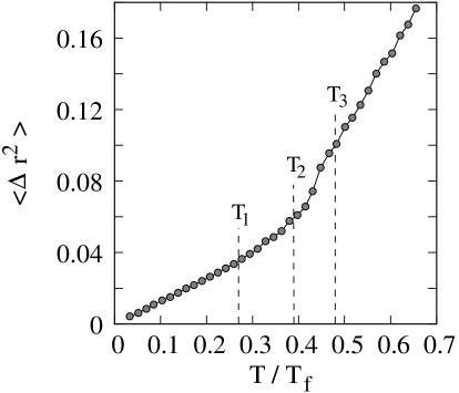
Figure 1: Average mean-squared distance fluctuations $\langle\Delta r^{2}\rangle$ as a function of temperature for protein G. Data adapted from nakagawa2 . The temperatures marked $T_{1}$, $T_{2}$, $T_{3}$ are the temperatures studied in Sec. IV.

Figure 1 shows the evolution of $\langle\Delta r^{2}\rangle$ as a function of temperature. It exhibits a crossover in the fluctuations in the temperature range $T/T_{f}=[0.4,0.5]$ resembling the transition observed for hydrated proteins in neutron scattering and Mössbauer spectroscopy experiments doster ; parak ; frauenfelder1 , the so-called dynamical transition. Above $T/T_{f}=0.4$, the fluctuations increase quickly with temperature whereas a smaller, linear, growth is observed below. One may wonder whether the complexity of the protein structure, reflected by the Gō model, is sufficient to lead to a dynamical transition or whether, notwithstanding the resemblance of the onset of fluctuations in the present model and the experimentally determined transition, different physical and not necessarily related events may contribute to the curves which by coincidence look similar. One can already note that, for a folding temperature in the range $330-350K$, the range $0.4-0.5\ T/T_{f}$ corresponds to $132-175K$, lower than the experimentally observed transition occurring around $180-200K$. If it had been confirmed the observation of a dynamical transition in a fairly simple protein model would have been very useful to shine a new light on this transition which is still not fully understood. It is generally agreed that it is hydration-dependent frauenfelder , but still different directions for a microscopic interpretation are being pursued, suggesting the existence chen or non-existence sokolov1 of a transition in the solvent coinciding at the dynamical transition temperature. Recently, a completely different mechanism based on percolation theory for the hydration layer has been proposed kataoka1 . The precise nature of the interaction between the solvent and proteins, and the driving factor behind the transition, hence still remain to be understood. The dynamical transition has often been called the protein glass transition due its similarity with some physical properties of structural glasses at low temperatures. In particular, it was pointed out that, for both glasses and protein solutions, the transition goes along with a crossover towards non-exponential relaxation rates at low temperatures. The comparison is however vague since the glass transition itself and notably its mechanism are ongoing subjects of research and debate.

Our goal in this paper is to clarify the origin of the numerically observed transition, which moreover gives hints on the possibilities and limits of protein computer models.

III Analysis of the incoherent structure factor

If computer models of proteins are to be useful they must go beyond a simple determination of the dynamics of the atoms, and make the link with experimental observations. This is particularly important for the “dynamical transition” because its nature in a real protein is not known at the level of the atomic trajectories. It is only observed indirectly through the signals provided by experiments. Therefore a valid analysis of the transition observed in the computer model must examine it in the same context, i.e. determine its consequences on the experimental observations.

Along with NMR and Mössbauer spectroscopy, neutron scattering methods have been among the most versatile and valuable tools to provide insight on the internal motion of proteins review1 ; smith91 . Indeed, the thermal neutron wavelength being of the order of Ångströms and the kinetic energy of the order of $meV$s, neutrons provide an adequate probe matching the length- and frequency scales of atomic motion in proteins. An aspect brought forward in the discussion of the dynamical transition in view of the properties of glassy materials is the existence of a boson peak at low frequencies in neutron scattering spectra doster99 . Such a broad peak appears to be a characteristic feature of unstructured materials as compared to the spectra of crystals.

III.1 Incoherent structure factor from molecular dynamics trajectories

In neutron scattering the vibrational and conformational changes in proteins appear as a quasielastic contribution to the dynamic structure factor $S(\mathbf{q},\omega)$ which contains crucial information about the dynamics on different time- and length scales of the system. In scattering experiments one measures the double-differential scattering cross section $d^{2}\sigma/(d\Omega dE)$ which gives the probability of finding a neutron in the solid angle element $d\Omega$ with an energy exchange $dE$ after scattering. The total cross-section of the experiment is obtained by integration over all angles and energies. Neglecting magnetic interaction and only considering the short-range nuclear forces, the isotropic scattering is characterized by a single parameter $b_{i}$, the scattering length of the atomic species $i$ bee , which can be a complex number with a non-vanishing imaginary part accounting for absorption of the neutron. If one defines the average over different spin states $b^{coh}=\left|\langle b\rangle\right|$ as the coherent scattering length, and the root mean square deviation $b^{inc}=\sqrt{\langle|b|^{2}\rangle-\left|\langle b\rangle\right|^{2}}$ as the incoherent scattering length, the double-differential cross section arising from the scattering of a monochromatic beam of neutrons with incident wave vector $\mathbf{k}_{0}$ and final wave vector $\mathbf{k}$ by $N$ nuclei of the sample can be expressed as bee

$$\frac{d^{2}\sigma}{d\Omega dE} = \frac{N}{\hbar}\frac{|\mathbf{k}|}{|\mathbf{k}_{0}|}\left(b^{coh}\right)^{2}S_{coh}(\mathbf{q},\omega)$$ (2)

$$+\frac{N}{\hbar}\frac{|\mathbf{k}|}{|\mathbf{k}_{0}|}\left(b^{inc}\right)^{2}S_{inc}(\mathbf{q},\omega)\ \ \ \ ,$$

where $\mathbf{q}=\mathbf{k}-\mathbf{k}_{0}$ is the wave vector transfer in the scattering process and $\mathbf{r}_{i}$ denote the time-dependent positions of the sample nuclei and the coherent and incoherent dynamical structure factors are

$$S_{coh}(\mathbf{q},\omega) =\frac{1}{2\pi N}\sum_{i,j}\int_{-\infty}^{\infty}dt\ e^{-i\omega t}\langle e^{-i\mathbf{q}(\mathbf{r}_{i}(t)-\mathbf{r}_{j}(0))}\rangle,$$ (3)

$$S_{inc}(\mathbf{q},\omega) =\frac{1}{2\pi N}\sum_{i}\int_{-\infty}^{\infty}dt\ e^{-i\omega t}\langle e^{-i\mathbf{q}(\mathbf{r}_{i}(t)-\mathbf{r}_{i}(0))}\rangle.$$ (4)

The coherent structure factor contains contributions from the position of all nuclei. The interference pattern of $S_{coh}(\mathbf{q},\omega)$ contains the average (static) structural information on the sample, whereas the incoherent structure factor $S_{inc}(\mathbf{q},\omega)$ monitors the average of atomic motions as it is mathematically equivalent to the Fourier transform in space and time of the particle density autocorrelation function. In experiments on biological samples, incoherent scattering from hydrogens dominates the experimental spectra smith91 unless deuteration of the molecule and/or solvent are used.

Since the Gō-model represents a reduced description of the protein and the locations of the individual atoms in the residues are not resolved, we use ”effective” incoherent weights of equal value for the effective particles of the model located in the position of the $C_{\alpha}$-atoms. Such a coarse grained view assumes that the average number of hydrogens atoms and their location in the residues is homogeneous, which is of course a crude approximation in particular in view of the extension and the motion of the side chains. These approximations are nevertheless acceptable here as we do not intend to provide a quantitative comparison with experimental results considering the simplifications and the resulting limitations of the model.

We generated Langevin and Nosé-Hoover dynamic trajectories of length $t=10^{5}$ time units, i.e. about 1000 periods of the slowest vibrational mode of the protein, after an equilibration of equal length for protein G at temperatures in the interval $T/T_{f}=[0.0459,0.9633]$. To compute the incoherent structure factor for the Gō-model of protein G, we use nMoldyn kneller to analyze the molecular dynamics trajectories generated at different temperatures. The data are spatially averaged over $N_{q}=50$ wave vectors sampling spheres of fixed modules $|\mathbf{q}|=2,3,4$ Å^-1, and the Fourier transformation is smoothed by a Gaussian window of width $\sigma=5\%$ of the full length of the trajectory. Prior to the analysis, a root-mean square displacement alignment of the trajectory onto the reference structure at time $t=0$ is performed using virtual molecular dynamics (VMD) vmd . Such a procedure is necessary in order to remove the effects of global rotation and translation of the molecule.

Figure 2 shows the frequency dependence of the incoherent structure factor $S(q,\omega)$ for a fixed wave vector $q=4$ Å^-1 for a simulation with the Nosé-Hoover thermostat. On Fig. 2-a, the evolution of the low frequency range of the structure is shown for a range of temperatures including the supposed dynamic transition region $T/T_{f}=[0.4,0.5]$. At low temperatures up to $T/T_{f}\approx 0.51$, individual modes are clearly distinguishable and become broadened as temperatures increases. The slowest mode, located around $4\;{\mathrm{cm}}^{-1}$ is also the highest in amplitude. It has a time constant of about $\tau=80$ in reduced units ($\approx 8\;$ps). These well-defined lines are observed to be shifting towards lower frequencies with increasing temperature, similar to the phonon frequency shifts that are frequently observed in crystalline solids. As we show in the following section, the location of these lines can be calculated from a harmonic approximation associated to a single potential energy minimum. Therefore, the shift in frequency and the appearance of additional modes can be seen as a signature of increasingly anharmonic dynamics involving several minima associated to different conformational substates.

(a)

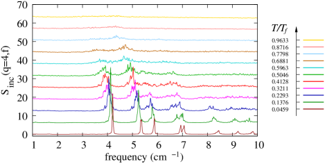
(b)

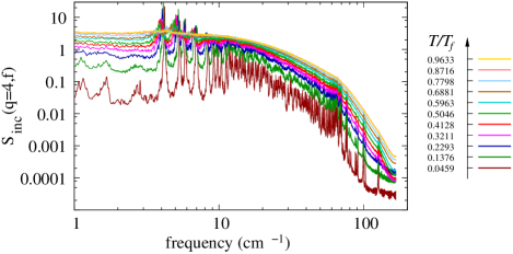
Figure 2: (Color online) Incoherent structure factor $S_{inc}(\mathbf{q}=4$ Å${}^{-1},\omega)$ as a function of temperature for protein G (Nosé-Hoover thermostat). The unit of time has been converted to absolute units using the approximate conversion factor $1\;$t.u. $=0.1\;$ps. Panel a) shows a magnification of the structure factor in the low frequency range. The structure factors on this panel have been shifted with an offset to avoid the overlap of curves at different temperatures. The different curves, from bottom to top, correspond to the temperatures $T/T_{f}$ listed on the side of each panel.

If, instead of the Nosé-Hoover thermostat, we consider the results obtained with Langevin dynamics and a friction constant $\gamma=0.01$, the stronger coupling to the thermostat leads to low energy modes which are significantly broader than with the Nosé-Hoover thermostat, so that they can hardly be resolved anymore. However the location of the peaks in the spectra remains the same as the one shown on Fig. 2-b. Besides the larger damping, Langevin calculations pose additional technical difficulties because Langevin dynamics does not preserve the total momentum of the system. The center of mass of the protein diffuses on the time scale of the trajectories. At low temperatures when fluctuations are small, the alignment procedure can efficiently eliminate contributions from diffusion as the center of mass is well defined for a rigid structure. At high temperatures however, it cannot be excluded that the alignment procedure adds spurious contributions to the structure factor calculations as the fluctuations grow in amplitude and the structure becomes flexible.

The analysis of the incoherent structure factor has shown that the low temperature dynamics of the Gō-model is dominated by harmonic contributions. An increase of temperature leads to a broadening and a shift of these modes until they eventually become continuously distributed. However, for both strong and weak coupling to the heat bath, no distinct change of behavior can be detected within the temperature range $T/T_{f}=[0.4,0.5]$ in which Fig. 1 shows an apparent dynamical transition. Instead, the numerical results suggest a continuous increase of anharmonic dynamics, and the absence of a dynamical transition in this model, even though, in the range $T/T_{f}=[0.4,0.5]$, the peaks of the structure factor in the Nosé-Hoover simulations broaden significantly. In the lowest temperature range the structure factor does not show any contribution reminiscent of a Boson peak.

III.2 Structure factor from normal mode analysis in the one phonon approximation

A further analysis can be carried out to determine whether the low temperature behavior of the protein model shows a complex glassy behavior or simply the properties of an harmonic network made of multiple bonds. The picture of a rough energy landscape of a protein with many minima separated by barriers of different height does not exclude the possibility that, in the low temperature range, the system behaves as if it were in thermal equilibrium in a single minimum of this multidimensional space. This would be the case if the time scale to cross the energy barrier separating this minimum from its neighbor basins were longer than the observation time (both in numerical or real experiments). In this case, it should be possible to describe the low temperature behavior of the protein in terms of a set of normal modes. To determine if this is true for the Gō model that we study, one can compare the spectrum obtained from thermalized numerical simulations at low temperature (low temperature curves on Fig. 2) with the calculation of the structure factor in terms of phonon modes, in the spirit of the study performed in ref. goupil-lamy for the analysis of inelastic neutron scattering data of staphylococcal nuclease at $25\;$K on an all-atom protein model.

The theoretical basis for a quantitative comparison is an approximate expression of the quantum-mechanical structure factor $S(\mathbf{q},\omega)$ in the so-called one-phonon limit which only accounts for single quantum process in the scattering events assuming harmonic dynamics of the nuclei. In this approximation, the incoherent structure factor can be written as

$$S_{inc}(\mathbf{q},\omega) =\sum_{i}\sum_{\lambda}b_{i}^{2}e^{\hbar\omega_{\lambda}\beta/2}e^{-2W_{i}(\mathbf{q})}\hbar|\mathbf{q.}\mathbf{e}_{\lambda,i}|^{2}$$

$$\times\left(4m_{i}\omega_{\lambda}\sinh(\beta\hbar\omega_{\lambda}/2)\right)^{-1}\delta(\omega-\omega_{\lambda})\ .$$ (5)

Here, the indices $i$ and $\lambda$ denote the atom and normal modes indices respectively. $\mathbf{e}_{\lambda,i}$ is the subvector relating to the coordinates of particle $i$ of the normal mode vector associated to index $\lambda$. $W_{i}(\mathbf{q})$ denotes the Debye-Waller factor, which in the quantum calculation of harmonic motion reads goupil-lamy

$$W_{i}(\mathbf{q}) = \sum_{\lambda}\frac{\hbar|\mathbf{q.}\mathbf{e}_{\lambda,i}|^{2}}{m_{i}\omega_{\lambda}}\left[2n(\omega_{\lambda})+1\right]\ \ \ ,$$ (6)

$n(\omega)$ being the Bose factor associated to the energy level $\omega$.

For the calculations of the structure factor in the Gō-model within this approximation, we average $S_{inc}(\mathbf{q},\omega)$ on a shell of $\mathbf{q}$-vectors by transforming the Cartesian coordinate vector $(q_{x},q_{y},q_{z})$ into spherical coordinates $\mathbf{q}=q\cdot\left(sin(\theta)cos(\phi),sin(\theta)sin(\phi),cos(\theta)\right)$, and generate a grid with $N_{q}$ points for the interval $\phi=[0,2\pi]$, and $N_{q}$ points for $\theta=[0,\pi]$. With this shell of vectors, we can evaluate the isotropic average $S_{inc}(q,\omega)$. In equation (5), $\hbar$ appears as a prefactor to the Debye-Waller factor $W_{i}(\mathbf{q})$ in the exponentials and in the inverse hyperbolic function. In order to evaluate the structure factor in reduced units of the Gō-model, we therefore need to estimate the order of $\hbar$ in a similar way as we did for the energy scale (see Appendix) by comparing the fractions

$$\frac{\hbar\omega}{k_{B}T_{f}} = \frac{\hbar^{\prime}\omega^{\prime}}{(k_{B}T_{f})^{\prime}}\ \ \ ,$$ (7)

the non-primed variables denoting quantities in reduced units. In the numerical evaluation of equation (5), we discretize the spectrum of frequencies from the smallest eigenvalue to the largest mode into $10000$ grid points to evaluate the $\delta$-function. We use $N_{q}=225$ vectors to average on a shell of modulus $|\mathbf{q}|=4$ Å^-1. The summation runs over all eigenvectors except for the six smallest frequencies which are numerically found to be close to zero, and result from the invariance to overall translation and rotation of the potential energy function.

In a first step, we use the coordinates of the global minimum of the Gō-model for protein G corresponding to the inherent structure with index $\alpha_{0}$ to calculate the Hessian of the potential energy function. The second derivatives are calculated by numerically differentiating the analytical first derivatives at the minimum. As discussed in the Appendix, due to the presence of frustration in the potential, the experimental structure does not correspond to the global minimum of the model. The difference between the minimum and the experimental structure is however small, with root-mean square deviation $0.16$ Å and notable changes in position occurring only for a small number of residues located in the second turn.

To estimate the normal mode frequencies in absolute units, we use the conversion of the time unit of $0.1\;$ps introduced in the Appendix. The conversion into wave numbers, which is convenient for the comparison to experimental data and to the results from all-atom calculations, is achieved by noting that, from $ck=f$, we can assign the conversion $1\;{\mathrm{ps}}^{-1}\rightarrow 33.3\;{\mathrm{cm}}^{-1}$ and multiply the frequencies by this scaling factor. Figure 3-a shows the results of the calculation of the incoherent structure factor $S(q=4$Å$,\omega)$ in the one phonon approximation at the temperature $T=0.0459\,T_{f}$. Since in this approximation the normal mode frequencies enter with a delta function into equation (5), there is no line width associated to these modes unless the structure factor is convoluted with an instrumental resolution function or a frictional model smith91 . Comparing to the structure factor calculated from a molecular dynamics trajectory at the same temperature (Fig. 3-b), we find a good correspondence of the location of the lines and their relative amplitude with respect to each other.

(a)

(b)

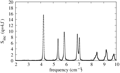
Figure 3: a) Frequency dependence of the incoherent structure factor $S(q=4$ Å$,\omega)$ ($T=0.0459\,T_{f}$) calculated from normal modes in the one-phonon approximation. This figure only shows the lower frequency part of the spectrum. b) Incoherent structure factor $S(q=4$ Å$,\omega)$ calculated from Nosé-Hoover constant temperature molecular dynamics at the same temperature.

Therefore the analysis of the incoherent structure factor using a harmonic approximation quantitatively confirms the dominant contribution of harmonic motion at low temperatures. In particular, the motion at very low temperatures occurs in a single energy well associated to one conformational substate. To see how this behavior changes with increasing temperature, in the next section we analyze the distribution of inherent structures with temperature.

IV Inherent structure analysis in the dynamic transition region

The freezing of the dynamics of a protein at temperatures below the “dynamic transition” is also described as a “glass transition”. This leads naturally to consider an energy landscape with many metastable states, also called “inherent states” in the vocabulary of glass transitions. In refs. nakagawa2 ; hagmann1 we showed that the thermodynamics of a protein can be well described in terms of its inherent structure landscape, i.e. a reduced energy landscape which does not describe the complete energy surface but only its minima. This picture is valid at all temperatures, including around the folding transition and above. For our present purpose of characterizing the low temperature properties of a protein and probe its possible relation with a glassy behavior, it is therefore useful to examine how the protein explores its inherent structure landscape in the vicinity of the dynamic transition. Here, we shall try to find how the number of populated minima changes with temperature around the transition region $T/T_{f}=[0.4,0.5]$ for the Gō-model of protein G, and which conformational changes can be associated to these inherent structures.

For three selected temperatures $T_{1}=0.275\ T_{f}$, $T_{2}=0.39\ T_{f}$, $T_{3}=0.482\ T_{f}$ shown on Fig. 1, we generated $10$ trajectories from independent equilibrated initial conditions for $2\cdot 10^{7}$ reduced time units using the Nosé-Hoover thermostat. Along each trajectory, a minimization was performed every $2\cdot 10^{4}$ time units such as to yield $N_{m}=20000$ minima for each temperature point. In the classification of these minima and their graphical representation, we only keep those minima which have been visited at least $2$ times within the $N_{m}$ minima, which lead to discard less than $10$ events from the total number of counts. Most of the counts are concentrated on a small number of inherent structures. In figure 4, we show the relative populations of the inherent structures on a two-dimensional subspace spanned by the inherent structure energy and the structural difference with the experimental structure measured by the dissimilarity factor nakagawa1 ; dissym . The radius of the circles centered at the location of the minima on this plane is set proportional to $1/2\ \log(w)$ where $w$ is the absolute number of counts of this minimum along the trajectories. This definition is necessary to allow the graphical representation on the plane, however, it may visually mask that linear differences in the radii translate into exponential differences of the frequency of visit of the minimum. As an example, the minima $\alpha_{0},\alpha_{1},\alpha_{2},\alpha_{3}$ have the occupation probabilities $p(\alpha_{0})=w(\alpha_{0})/N_{m}\approx\ 92\%$, $p(\alpha_{1})\approx\ 8\%$, $p(\alpha_{2})\approx\ 0.1\%$ and $p(\alpha_{3})\approx\ 0.02\%$ at $T=T_{1}$.

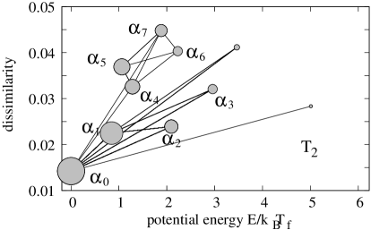
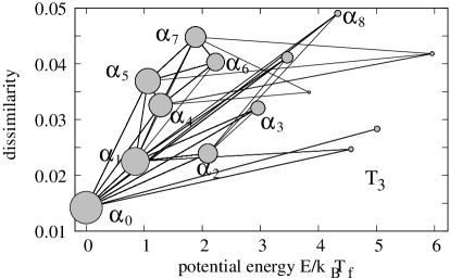
Figure 4: Inherent structure population of the Gō-model for protein G at temperatures $T_{1},T_{2},T_{3}$ (from top to bottom) and their associated structural dissimilarity. Lines are drawn between states that are connected within a MD trajectory. The width of the circles is proportional to $1/2\ log(w)$ where $w$ is the total number of occurrences of a given minimum.

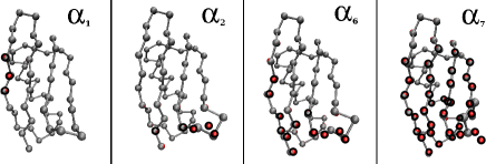
Figure 5: (Color online) Shapes of inherent structures $\alpha_{1}$, $\alpha_{2}$, $\alpha_{6}$, $\alpha_{7}$. The reference coordinates of the global minimum $\alpha_{0}$ are shown by red balls surrounded by a thick black line. The coordinates of the global minimum are invisible for residues which overlap with the inherent structure coordinates.

From figure 4, we notice that already at $T_{1}$ more than one minimum is populated though the global minimum $\alpha_{0}$ is dominant. In these figures, lines are drawn between minima that are connected along the trajectory, i.e. that form a sequence of events. It should however be noted that since the sampling frequency is low, it cannot be excluded that an intermediate corresponding to an additional connection line is skipped. Connections between all minima may therefore exist even though they did not appear in the sequences observed in this study. Moving to higher temperatures $T_{2}$ and $T_{3}$, a larger number of minima which are both higher in energy and structural dissimilarity appear. As the temperature rises, their population numbers become more important, as can be seen e.g. by inspection of the radii of the block $\alpha_{4}$-$\alpha_{7}$ on figure 4. To obtain a physical picture of the conformational changes associated with these minima, it is useful to align their coordinates onto the coordinates of the global minimum. The results of such an alignment are shown in figure 5. In this figure, the coordinates of the effective Gō-model particles located at the positions of the $C_{\alpha}$-atoms for each amino-acid are drawn in red color. One notices that the conformational changes associated to $\alpha_{1}$-$\alpha_{3}$ are small. It is interesting to notice that these small changes already appear in the range of temperatures where the rise in fluctuations seems to grow still linearly with the temperature. The next higher minima involve in particular a reorientation of a turn within the $\beta$-sheets of a protein. The temperature range at which these minima start to be populated coincides with the transition region revealed by the mean-distance displacement $\langle\Delta r^{2}\rangle$, suggesting that the anharmonic motion required to make transitions between the basins of these minima is at its origin.

We again observe that the dynamic transition region does not exhibit any particular change of behavior that could deserve the name of “transition”, but rather a gradual evolution which gets noticeable in the range $T/T_{f}=[0.4,0.5]$. In the next section we use a non-equilibrium approach to reveal whether the dynamics below the transition range can be characterized as ”glassy” or not.

V Test of the fluctuation-dissipation theorem (FDT) - a non-equilibrium approach

An alternative approach to study the low temperature transition, for which equilibrium simulations take a significant amount of computer time, consists in the test of the response of the protein to external perturbations. Rather than waiting a long time to see rare fluctuations dominating the average fluctuation at low temperatures, the system is driven out of equilibrium on purpose to either observe the relaxation back to equilibrium and its associated structural changes, or the response to a continuous perturbation to be compared to fluctuations at equilibrium.

The fluctuation-dissipation theorem (FDT) relates the response to small perturbations and the correlations of fluctuations at thermal equilibrium for a given system. In the past years, the theorem and its extensions have become a useful tool to characterize glassy dynamics in a large variety of complex systems crisanti . For glasses below the glass transition temperature, the equilibrium relaxation time scales are very large so that thermal equilibrium is out of reach berthier . Consequently, the FDT cannot be expected to hold in these situations, and the response functions and correlation functions in principle provide distinct information. In this section, we test the FDT for the Gō-model of protein G at various temperatures to see whether a signature of glassy dynamics is present in the system. To this aim, we first recall the basic definitions and notations for the theorem.

In our studies we start from a given initial condition and put the system in contact with a thermostat during a waiting time $t_{w}$. The end of the waiting time is selected as the origin of time ($t=0$) for our investigation. If $t_{w}$ is large enough (strictly speaking $t_{w}\to\infty$) the system is in equilibrium at $t=0$. We denote the Hamiltonian of the unperturbed system $H_{0}$, which under a small linear perturbation of the order $\epsilon(t)$ acting on an observable $B(t)$ becomes

$$H = H_{0}-\epsilon(t)B(t)\ \ \ ,$$ (8)

where for $\epsilon=0$ we recover the unperturbed system. For any observable $A(t)$, we accordingly define the two ensemble averages $\langle A(t)\rangle_{0}^{t_{w}}$ and $\langle A(t)\rangle_{\epsilon}^{t_{w}}$ where the index references the average with respect to the unperturbed/perturbed system respectively and the exponent $t_{w}$ indicates how long the system was equilibrated before the start of the investigation. The correlation function in the unperturbed system relating the observables $A(t)$, $B(t^{\prime})$ at two instances of time $t,t^{\prime}$ is defined by

$$C_{AB}(t,t^{\prime}) = \langle A(t)B(t^{\prime})\rangle_{0}^{t_{w}}-\langle A(t)\rangle_{0}^{t_{w}}\;\cdot\langle B(t^{\prime})\rangle_{0}^{t_{w}}\ \ \ .$$ (9)

The susceptibility $\chi_{AB}(t)$, which measures the time-integrated response of the of the observable $A(t)$ at the instant $t$ to the perturbation $\epsilon(t^{\prime})$ at the instant $t^{\prime}$, reads

$$\chi_{AB}(t) = \int_{t_{0}}^{t}dt^{\prime}\ \frac{\delta\langle A(t)\rangle_{\epsilon}^{t_{w}}}{\delta\epsilon(t^{\prime})}\ \;.$$ (10)

The index $B$ in the susceptibility indicates that the response is measured with respect to the perturbation arising from the application of $B(t)$, and the lower bound $t_{0}$ of the integral indicates the instant of time at which the perturbation has been switched on.

The integrated form of the FDT states that the correlations and the integrated response are proportional and related by the system temperature at equilibrium

$$\chi_{AB}(t)=\frac{1}{k_{B}T}\;\Delta C\quad\mathrm{with}$$

$$\Delta C=\left(C_{AB}(t,t)-C_{AB}(t,0)\right)\ \ .$$ (11)

In the linear response regime for a sufficiently small and constant field $\epsilon$, the susceptibility can be approximated as

$$\chi_{AB}(t) \approx \frac{\langle A(t)\rangle_{\epsilon}^{t_{w}}-\langle A(t)\rangle_{0}^{t_{w}}}{\epsilon}$$ (12)

such that in practice, verifying the FDT accounts for the comparison of observables on both perturbed and unperturbed trajectories.
 
The basic steps for a numerical experiment aiming to verify the FDT can be summarized as follows:

• Initialize two identical systems 1 and 2; 1 to be simulated with and 2 without perturbation.

• Equilibrate both systems without perturbation during $t_{w}$.

• At time $t_{0}$ (in practice $t_{0}=0$, i.e. immediately after the end of the equilibration period) switch on the perturbation for system 1 and acquire data for both systems for a finite time $t_{\mathrm{FDT}}$.

• Repeat the calculation over a large number of initial conditions to yield the ensemble averages $\langle\cdot\rangle_{0}^{t_{w}}$ and $\langle\cdot\rangle_{\epsilon}^{t_{w}}$; combine the data according to equation (11).

The protocol may be modified to include an external perturbation which break the translational invariance in time. For instance the initial state can result from a quench from a high to a low temperature. Then the system is only equilibrated for a short time $t_{w}$ before the perturbation in the Hamiltonian is switched on. In this case the distribution of the realizations of the initial conditions is not the equilibrium distribution so that the correlation function defined by Eq. (9) depends on the two times $t$ and $t^{\prime}$ and not only on their difference.

V.1 Simulation at constant temperature

This case corresponds to $t_{w}\to\infty$. In our calculations we start from an initial condition which as been thermalized for at least $5000\;$ time units. The first step is to make an appropriate choice for the perturbative potential $\epsilon(t)B(t)$. An earlier application of the FDT to a protein model hayashi has used the perturbative term

$$\epsilon(t)B(t)=\epsilon\sum_{i=1}^{N}\cos(k\;y_{i})\;,$$ (13)

where $k$ is a scalar, $y_{i}$ the $y$ coordinate of amino-acid $i$ and $\epsilon\not=0$ for $t>t_{0}$ a constant. This perturbation is invariant neither by a translation of the system nor by its rotation. Although this does not invalidate the FDT, this choice poses some problems for the accuracy of the calculations because, even in the absence of internal dynamics of the protein, the perturbation varies as the molecules diffuse in space or rotate. To avoid this difficulty we selected the perturbation

$$W:=-\epsilon B(t)=-\epsilon\sum_{i=1,i\not=28}^{N}\cos(k\;r_{i,28})\;,$$ (14)

where $r_{i,28}$ is the distance between amino-acid $i$ and the amino-acid $28$ which has been chosen as a reference point within the protein because it is located near the middle of the amino-acid chain. Such a potential only depends on the internal state of the molecule, while it remains unaffected by its position in space. To test the FDT for the Gō-model of protein G using Eqs. (11) and (12), we add this potential $W$ to the potential energy $V$ of the model and we select $A(t)=B(t)$. The thermal fluctuations are described with the same Langevin dynamics as previously. We switch on the perturbation for the equilibrated protein model and record $50000$ to $400000$ trajectories (depending on the value of $\epsilon$) of duration $2000$ time units for temperatures in the range $T/T_{f}=[0.275,0.826]$ covering both the low temperature domain and the approach of the folding transition of the protein. The perturbation prefactors chosen in this first set of simulations were $\epsilon=0.05$ and $\epsilon=0.005$, and the wave number of the cosine-term was $k=2\pi/10$.

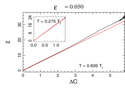
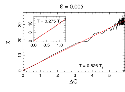
Figure 6: (Color online) Variation of $\chi$ versus $C$ for $\epsilon=0.05$ and $\epsilon=0.005$ at the equilibrium temperature $T=0.826\,T_{f}$. The insets show $\chi$ versus $\Delta C$ at $T=0.275\,T_{f}$. The oblique (red) lines show the slope $1/k_{B}T$ that would be expected according to the fluctuation-dissipation theorem. The results presented on this figure have been obtained from 400000 realizations.

Figure 6 shows the evolution of the relation between the susceptibility and the variation of the correlation function $\Delta C=C_{AB}(t,t)-C_{AB}(t,0)$. The straight lines represent the slopes expected from the FDT. One notices that, for $\epsilon=0.05$, at $T=0.826\,T_{f}$, in the long term the value of $\chi/\Delta C$ stabilizes around a value which is away from the expected value $1/k_{B}T$. From a first glance, this result is reminiscent of the properties of a glass driven out of equilibrium. In this context, the deviation from the slope expected from the FDT is interpreted as the existence of an ”effective temperature” for non-equilibrium systems. For the case studied here, finding an effective temperature would be surprising as the results are obtained from measurements on a thermalized protein model, i.e. a system in a state of thermal equilibrium. How is it then possible to explain the apparent deviation from the FDT? The calculations performed with $\epsilon=0.005$ give the clue because they show that the deviation appeared because the perturbation was too large and outside of the linear response regime assumed to calculate the susceptibility because for this lower value of $\epsilon$ the deviation has vanished. If one computes the average value of the perturbation energy $\langle W\rangle$ and compares it to the protein average energy $\langle E(T)\rangle$, for the case shown on Fig. 6, $\epsilon=0.05$, one finds $\langle W\rangle/\langle E(T)\rangle=1.3\cdot 10^{-2}$. This is small, but, at temperatures which approach $T_{f}$ the protein is a highly deformable object and even a small perturbation can bring it out of the linear response regime. This shows up by the the a rise of $\chi$ versus time for $\epsilon=0.05$. At low temperatures the protein is more rigid an therefore more resilient to perturbations. The insets on Fig. 6 show that for $\epsilon=0.05$ the calculations find that the fluctuation-dissipation relation at $T=0.275\,T_{f}$ is almost perfectly verified although a very small deviation can still be detected for this value of $\epsilon=0.05$. Therefore a careful choice of parameters is necessary to test the FDT under controlled conditions. In particular, the perturbation needs to be carefully chosen to only probe the internal dynamics and not to dominate them.

V.2 Simulation of quenching

A typical signature of a glassy system is its aging after a perturbation. In the context of the protein “glass transition”, one can therefore expect to detect a slow evolution of the system as a function of the time after which it has been brought to the glassy state. This is usually tested in quenching experiments, which can be investigated by a sharp temperature drop in the numerical simulations. Our calculations start from an equilibrium state at high temperature $T=1.40\,T_{f}$, which is abruptly cooled at a temperature $T_{q}$ below the temperature of the dynamical transition studied in the previous sections. The model protein is then maintained at this temperature $T_{q}$ by a Langevin thermostat. After a waiting time $t_{w}$ we start recording the properties of the system over a time interval $t_{\mathrm{FDT}}=25000\;$t.u. to probe the fluctuation dissipation relation. In order to avoid nonlinear effects we use a small value of $\epsilon=0.005$. For such a weak perturbation, the response is weak compared to thermal fluctuations and a large number of realizations ($50000$ or more) is necessary to achieve reliable statistical averages. To properly probe the phase space of the model, these averages must be made over different starting configurations before quenching. This is achieved by starting the simulations from a given initial condition properly thermalized at $T=1.40\,T_{f}$ in a preliminary calculation. Then we run a short simulation at this initial temperature, during which the unfolded conformations change widely from a run to another with different random forces because at high temperatures the fluctuations of the protein are very large. The conformations reached after this short high-$T$ thermalization are the conformations which are then quenched to $T_{q}$, for the FDT analysis.

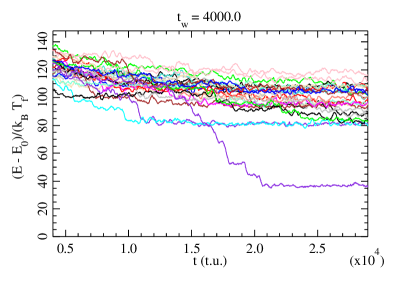
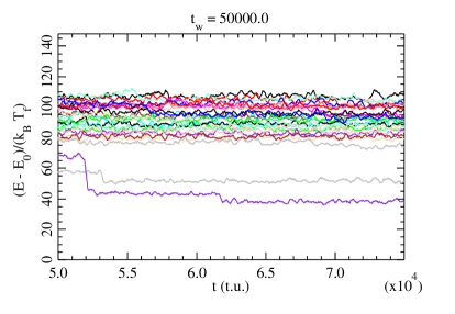
Figure 7: (Color online) Time evolution of the energy above the ground state, in units of $k_{B}T_{f}$, after a temperature jump from $T=1.4\,T_{f}$ to $T=0.367\,T_{f}$ for two different waiting times $t_{w}$, indicated in the title of each panel. The figure shows the evolution of the energy for 15 realisations (corresponding to the different colors) for the time $t_{\mathrm{FDT}}=25000\;$t.u.

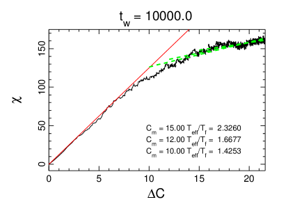
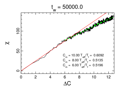
Figure 8: (Color online) Test of the FDT for the temperature jump from $T=1.4\,T_{f}$ to $T=0.367\,T_{f}$ and different waiting times $t_{w}$, indicated in the title of each panel. The figures show the response function $\chi$ versus the variation $\Delta C$ of the correlation function. The full straight lines (red) show the result of the FDT. The results for $t_{w}=10000\;$t.u. have been obtained by averaging over 115000 independent realizations, those for $t_{w}=50000\;$t.u. have been obtained with 92000 realizations. The dotted (green) lines show the fit of the data for the domain $\Delta C>C_{m}$ where $C_{m}$ is the value above which the curve deviates significantly from the line of slope $1/T$. The inverse of the slope of these fits defines an effective temperature $T_{\mathrm{eff}}$. As indicated in the legend of each figure, the value obtained for $T_{\mathrm{eff}}$ slightly depends on the choice of $C_{m}$. By varying $C_{m}$ we can therefore estimate the standard deviation on the value of $T_{\mathrm{eff}}$.

Typical results are shown on Figs. 7 and 8 for two values of $t_{w}$. The time evolution of the energy shows that, after the waiting time $t_{w}$, even for the largest value $t_{w}=50000\;$t.u. the model protein is still very far from equilibrium because its energy is well above the ground state energy (chosen as the reference energy $0$). This non-equilibrium situation sometimes leads to rapid energy drops, generally accompanied by a decrease of the dissimilarity with the native state, which superimpose to random fluctuations which have to be expected for this system in contact with a thermal bath. As expected the sharp variations of the conformations are more noticeable for the shortest waiting time. Figure 8 shows that, while for small values of $\Delta C=\left(C_{AB}(t,t)-C_{AB}(t,0)\right)$, which also correspond to shorter times after we start to collect the data for the FDT test, the variation of $\chi_{AB}(t)$ versus $\Delta C$ follows the curve given by the FDT relation, then at larger $\Delta C$ the curve shows a significant deviation from the slope $1/T$, which defines an effective temperature $T_{\mathrm{eff}}>T$. The effective temperature is larger for short waiting times after the quench and decreases when $t_{w}$ increases. This should be expected because, in the limit $t_{w}\to\infty$ we should have $T_{\mathrm{eff}}\to T$ when the system reaches equilibrium.

It is not surprising to find a deviation from the FDT behavior after a strong quench of the protein model because we put the system very far from equilibrium. Therefore the observation of an effective temperature that differs from the actual temperature of the system is not a sufficient indication to conclude at the existence of a glassy state of the protein model. What is important is the timescale at which the system tends to equilibrium and how it depends on temperature. To study this we have performed a systematic study of the variation of $T_{\mathrm{eff}}(t_{w};T)$ as a function of the waiting time $t_{w}$ and temperature $T$, at the temperatures $T=0.1875\,T_{f}$, $T=0.2752\,T_{f}$, $T=0.3670\,T_{f}$, $T=0.4128\,T_{f}$ and $T=0.4817\,T_{f}$. The temperature domain that we can study numerically is limited both from below and from above. At the lowest temperatures the relaxation of the system is very slow so that $t_{w}$ must be strongly increased. Moreover the speed at which the protein model explores its phase space by moving from an inherent structure to another becomes very low and statistically significant data cannot be obtained without a large increase of $t_{\mathrm{FDT}}$. Running enough calculations to get a good average on the realizations becomes unpractical. As discussed above, at high temperatures the protein becomes “soft” so that one quickly leaves the linearity domain of the FDT, unless the applied perturbation becomes very small. But then the large thermal fluctuations reduce the signal to noise ratio. Therefore the advantage of faster relaxation times at high temperature is whipped out by the need to make statistical averages over a much larger number of realizations. However the temperature range over which one can get statistically significant results overlaps the temperature $T\approx 0.45\,T_{f}$ above which the fluctuations of the model appear to grow faster (Fig. 1) so that one could expect to observe a change in the properties of the system at this temperature, if it existed.

Figure 9: Variation of the effective temperature $T_{\mathrm{eff}}$ as a function of the waiting time $t_{w}$ at two temperatures, $T=0.2572\,T_{f}$ (open circles) and $T=0.4128\,T_{f}$ (closed squares). The figure shows $\ln\left({T_{\mathrm{eff}}}/{T}-1\right)$ versus $t_{w}$. The lines show a linear fit that takes into account the error bars on the determination of $T_{\mathrm{eff}}$ determined as explained in the caption of Fig. 8. Such a fit determines $\tau(T)$ and its the standard deviation. For $T=0.4128\,T_{f}$ the point corresponding to the largest value of $t_{w}$ is not included in the fit (see the discussion in the text).

At a given temperature $T$ we have defined a relaxation time $\tau(T)$ by assuming that the effective temperature relaxes exponentially towards the actual temperature according to

$$\left(\frac{T_{\mathrm{eff}}}{T}-1\right)\propto\exp\left(-\frac{t_{w}}{\tau(T)}\right)\;.$$ (15)

Figure 9 shows that this assumption is well verified by the numerical calculations. It should however be noticed that, for the longest waiting times, we may observe a large deviation from the exponential decay, as shown in Fig. 9 for the results at $T=0.4128\,T_{f}$. We attribute this to the limitations of our observations because, when the system has sufficiently relaxed so that its effective temperature approaches the actual temperature, all subsequent relaxations become extremely slow and may exceed the observation time $t_{\mathrm{FDT}}=25000\;$t.u. so that the test of the FDT no longer properly probes the phase space. Increasing $t_{\mathrm{FDT}}$ by an order of magnitude might allow us to observe the relaxation further but is beyond our computing possibilities as we have to study at least $50000$ realizations or more to achieve a reasonable accuracy. A fit of the values of $\left({T_{\mathrm{eff}}}/{T}-1\right)$ versus $t_{w}$, which takes into account the statistical weight of each point according to its standard deviation obtained from the uncertainties on $T_{\mathrm{eff}}$ determines the relaxation time $\tau(T)$ and its corresponding standard deviation.

Figure 10: Variation of the relaxation time $\tau(T)$ versus temperature. We plot $\ln(\tau)$ versus $T_{f}/T$. The line is a fit of the values which takes into account the uncertainties on the values of $\tau(T)$.

Figure 10 shows the variation of $\tau(T)$ with temperature, in logarithmic scale, versus $T_{f}/T$. It shows that, except for the value at the lowest temperature $T=0.1875\,T_{f}$, i.e. $T_{f}/T=5.45$, within the numerical errors evaluated at each stage of our calculation, the relaxation time obeys a standard Arrhenius relation

$$\tau(T)=\tau_{0}\exp\left(\frac{E_{a}}{T}\right)$$ (16)

with an activation energy $E_{a}/(k_{B}T_{f})=0.5668\pm 0.1799$. At the lowest temperature, the relaxation temperature estimated from the Arrhenius law is $\tau(T=0.1875\,T_{f})\approx 100000\,$t.u. so that calculations with $t_{w}\geq 100000$ as well as $t_{\mathrm{FDT}}\gg 100000$ would be necessary, which is unpractical. However the observed deviation from Arrhenius law at low $T$ cannot be attributed to a low-temperature glass transition because such a transition would lead to a relaxation time larger than predicted by the Arrhenius relation, while we observe the opposite. In any case the Arrhenius relation is well verified for a temperature range which overlaps the temperature $T\approx 0.45\,T_{f}$, i.e. $T_{f}/T\approx 2.22$, above which dynamical simulations suggested a possible increase of the fluctuations (Fig. 1). Therefore the relaxation of the protein model after a quench appears to follow a standard activated process, with an activation energy of the order of $0.57\;k_{B}T_{f}$, without any sign of a glassy behavior.

These observations can be compared with other studies of the fluctuations of the same Gō model of protein G nakagawa2 ; NakagawaPRL . Paper [nakagawa2, ] investigated the fluctuation in equilibrium below the folding temperature $T_{f}$. In these conditions, the numerical simulations of a protein which is near its native state detect small, up and down, jumps of the dissimilarity factor, which, in any case, stays very low ($d\approx 0.06$ for the equilibrium temperature $T=0.55\,T_{f}$) but switches between values that differ by $\approx 0.01$. In its equilibrium state the protein may jump from an inherent structure to another but these fluctuations are much slower than the one that we observed shorter after a temperature quench because they occur on a time scale of the order of $10^{7}\;$t.u. Their activation energy had been found to be $E_{B}=6.2\,T_{f}$, i.e. much higher than the activation energy $E_{a}$ that characterizes the relaxation of the effective temperature that we measured. Those results are not in contradiction because they correspond to fundamentally different phenomena. The non-equilibrium fluctuations that we discuss in the present paper appear because the potential energy surface has minima on the side of the “funnel” that leads to the native state. Such minima, corresponding to protein structures which are not fully folded, can temporarily trap the protein in intermediate states. However the lifetime of these high-energy minima is only of the order of $10^{5}\;$t.u. i.e. they are short lived compared to the residence time of the protein in an inherent structure close to the native state. When the protein escapes from one of these high-energy minima we observe an energy drop, as shown in Fig. 7.

The study that we presented here is neither a study of the protein near equilibrium, nor an investigation of the full folding process which also occurs on much longer time scales (typically $10^{7}$–$10^{8}\;$t.u.) as observed in Refs. [nakagawa2, ] and [NakagawaPRL, ]. Therefore the activation energy $E_{a}$ is also different from the energy barrier for folding. For the same reason the effective temperature after the quench $T_{\mathrm{eff}}$ should not be confused with the configurational temperature $T_{\mathrm{cnf}}$ defined in Ref. [NakagawaPRL, ] which relates the entropy and energy of the inherent structures during folding. $T_{\mathrm{cnf}}$ gives a global view of the phase space explored during folding, and it evolves with a characteristic time of $10^{7}$–$10^{8}\;$t.u. as the folding itself. Compared to these scales, the FDT analysis that we presented here appears as a snapshot of the strongly non-equilibrium state created after a fast quench. It offers a new view of the time evolution of the protein model, which completes the ones which had been presented earlier.

VI Discussion

The starting point of our study has been the numerical observation of a low temperature transition in a simplified protein model resembling the experimentally observed dynamical transition in hydrated protein samples. This suggested that, in spite of its simplicity, the frustrated Gō model could be used not only to study the folding of proteins but also their dynamics in the low temperature range, opening the way for an exploration of the glassy behavior of proteins.

We have therefore used different approaches to further characterize the properties of the protein model in the low temperature range. Thermalized molecular dynamics simulations have been used to calculate the incoherent structure factor than one could expect to observe for the protein. It shows peaks that broaden as temperature increases, suggesting that the dynamics of the protein model is dominated by harmonic or weakly anharmonic vibrations. This has been confirmed by the calculation of the structure factor in the one-phonon approximation. All the main features of the structure factor obtained by simulations, such as the peak positions and even the power law decay of the amplitude of the modes with frequency, are well reproduced. In the low temperature range, the dynamics of the protein appears to occur in a single energy well of its highly multidimensional energy landscape. Of course this is no longer true when the temperature increases.

By analyzing the population of the inherent structures, we have shown that, in the temperature range of the dynamical transition, there is a continuous increase of the number of states which are visited by the protein. The transition seems to be continuous, and it is likely that numerical observations suggesting a sudden increase may have the origin in the limited statistics due to finite time observation. Indeed, as shown for the example of protein G, the conformational transitions become extremely slow at low temperatures, such that the waiting time between the jumps between conformations may exceed the numerical (or the experimental) observation time. It is this breakdown of the ergodic hypothesis together with the observation of non-exponential relaxation rates which may have lead to the emergence of the terminology ”protein glass transition” in analogy to the phenomenology of glasses.

Non equilibrium studies allowed us to systematically probe a possible glassy behavior by searching for violations of the fluctuation–dissipation theorem. First we have shown that these calculations must be carried out with care because apparent violations are possible, even when the system is in equilibrium, due to nonlinearities in the response. Except at very low temperatures they can be observed even for perturbations as low as 1% of the potential energy of the system. Once this artifact is eliminated by the choice of a sufficiently small perturbative potential, we have shown that, after a sudden quench from an unfolded state to a very low temperature $T_{q}$, one does observe a violation of the FDT in the protein model, analogous to what is found in glasses. The quenched protein is characterized by an effective temperature $T_{\mathrm{eff}}>T_{q}$. But the relaxation of the model towards equilibrium, deduced from the evolution of the effective temperature $T_{\mathrm{eff}}$ as a function of the waiting time after the quench, follows a standard Arrhenius behavior, even when the temperature crosses the value $T\approx 0.45T_{f}$ at which dynamical simulations appeared to show a change in the amplitude of the fluctuations.

Although one cannot formally exclude that the results could be different for other protein structures or other simplified protein models, this work concludes that a coarse-grain model such as the Gō model is too simple to describe the complex behavior of protein G and particularly its glass transition. Indeed such a model does not include a real solvent, which plays an important role in experiments. The thermostat used in the molecular dynamics simulations only partially models the effect of the surrounding of the protein. The apparent numerical transition previously observed for protein G may simply be related to finite-time observations of the activation of structural transitions which appears in a particularly long time scale for proteins. This is an obvious limitation of molecular dynamics calculations, but this could also sound as a warning to experimentalists. Indeed experiments can access much longer time scales. But they also deal with real systems which are much more complex than the Gō model. In these systems relaxations may become very long, so that the experimental observation of a transition could actually face the same limitations as the numerical simulations. Such a ”time window” interpretation has also been brought forward for the experimentally observed dynamical transition, suggesting that the transition may in fact depend on the energy-, and thus, on the time-resolution of the spectrometer becker . In this respect, as shown by our non-equilibrium studies to test the validity of the FDT, such measurements, if they could be performed for a protein should tell us a lot about the true nature of the “glass transition” of proteins.

*

Appendix A Simulation and units

The forcefield and the parametrization of the simplified Gō-model are presented in nakagawa2 ; nakagawa1 . In a standard Gō model the potential energy is written in such a way that the experimental energy state is the minimal energy state. We use here a weakly frustrated Gō model for which the dihedral angle potential does not assume a minimum in the reference position defined by the experimentally resolved structure: it favors angles close to $\pi/4$ and $3\pi/4$ irrespective of the secondary structure element (helix, sheet, turn) the amino acid belongs to. This source of additional ”frustration” affects the dynamics and thermodynamics of the model, leading to a more realistic representation nakagawa1 . This feature introduces additional complexity in the model because, besides its ground state corresponding to the experimental structure, the frustrated model exhibits another funnel for folding, which leads to a second structure which is almost a mirror image of the ground state, but has a significantly higher energy (Fig. 11).

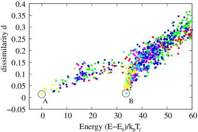
Figure 11: Stable and metastable conformations of the protein $G$ model obtained by a non-equilibrium cooling protocol followed by energy minimization (the various colors show minima obtained with different speed of cooling). The horizontal axis shows the energy of each structure with reference to the global minimum, and the vertical axis indicates its dissimilarity with the ground state nakagawa1 ; dissym , lower values indicating more structural similarities between two conformations.

To control temperature in the molecular dynamics simulations, several types of numerical thermostats were used. Most of the calculations use underdamped Langevin simulations bbk ; Honeycutt with a time step $dt=0.1\;$t.u. and friction constants in the range $\gamma=0.01,0.025$. The mass of all the residues is assumed to be equal to $m=10$. Some calculations were also performed with the multi-thermostat Nose-Hoover algorithm using the specifications defined in martyna .

For simulation purposes, the variables in the Gō-model are chosen dimensionless (reduced units). Lengths are expressed in units of $\tilde{l}=1$ representing Ångströms, and the average mass of an amino-acid, $135\;$Da, has been expressed as $10$ units of mass of the model. As the empirical potentials are defined at the mesoscopic scale of the amino-acids, values for the interaction constants in the effective potentials cannot be easily estimated in absolute units. It is possible to estimate the energy scale of the model by comparing the reduced folding temperature of the Gō-model with a realistic order of magnitude of the folding temperature $T^{\prime}_{f}$ in units of $K$ and setting

$$k^{\prime}_{B}T^{\prime}_{f} = \tilde{\epsilon}k_{B}T_{f}\ \ \ \ ,$$ (17)

where the variables on the left-hand side are given in SI units ($T^{\prime}_{f}$ is the estimate of the folding temperature), and unprimed variables are written in reduced units; $\tilde{\epsilon}$ is the required energy scale in units of $J$ to match between both. In our calculations $k_{B}=1$ (meaning that reduced temperatures are expressed in reduced energy units) and $T_{f}=0.218$ is deduced from equilibrium simulations. Then a simple dimensional analysis gives the time unit of the model as $\tilde{t}=\sqrt{\frac{\tilde{m}\tilde{l}^{2}}{\tilde{\epsilon}}}\ .$ One arrives at an estimated time unit of $\tilde{t}\approx 0.1\;$ps. In the paper we refer to $\tilde{t}\approx 0.1\;$ps as the unit of time (t.u.) for the simulations of the Gō-model, keeping in mind that this can merely be seen as an order of magnitude in view of the approximations that lead to this number.

References

- (1) K. Henzler-Wildman and D. Kern, Nature 450 964-972 (2007)
- (2) W. Doster, S. Cusack, and W. Petry, Nature 337, 754 (1989)
- (3) F. Parak, E. N. Frolov, R. L. Mossbauer, and V. I. Goldanskii, J. Mol. Biol. 145, 825 (1981)
- (4) Frauenfelder H, Petsko GA and Tsernoglou D, Nature, 280, 558 (1979)
- (5) H. Frauenfelder, S.G. Sligar and P.G. Wolynes, Science 254, 1598 (1991)
- (6) J.D. Bryngelson, J.N. Onuchic, N.D. Socci and P.G. Wolynes, Proteins: Struct. Funct. Genetics 21, 167 (1995)
- (7) C. Clementi, H. Nymeyer and J.N. Onuchic, J. Mol. Biol, 298, 937 (2000)
- (8) J. Karanicolas and C.L. Brooks, J. Mol. Biol. 334, 309 (2003)
- (9) N. Nakagawa and M. Peyrard; Proc. Natl. Acad. Sci. USA 103, 5279 (2006)
- (10) N. Nakagawa and M. Peyrard, Phys. Rev. E 74, 041916 (2006)
- (11) J.-G. Hagmann, N. Nakagawa and M. Peyrard, Phys. Rev. E 80, 061907 (2009)
- (12) A.M. Gronenborn, D.R. Filpula, N.Z. Essig, A. Achari, M. Whitlow, P.T. Wingfield, and G.M. Clore, Science 253, 657 (1991)
- (13) Fenimore PW, Frauenfelder H, McMahon BH and Young RD 2004 Proc. Nat. Acad. Sci. USA 101 14408
- (14) S.-H.Chen, L. Liu, E. Fratini, P. Baglioni, A. Faraone, and E. Mamontov, Proc. Natl. Acad. Sci. USA 103, 9012 (2006)
- (15) S. Pawlus, S. Khodadadi and A.P. Sokolov, Phys. Rev. Lett. 100, 108103 (2008)
- (16) H. Nakagawa, M. Kataoka, J. Phys. Soc. Jpn 79 083801 (2010)
- (17) F. Gabel et al., Quart. Rev. Biophys. 35, 4 (2002)
- (18) J.C. Smith, Quart. Rev. Biophys. 24, 3 (1991)
- (19) Leyser H, Doster W and Diehl M 1999 Phys. Rev. Lett. 82 2987
- (20) M. Bée, Quasielastic Neutron Scattering: Principles and Applications in Solid State Chemistry, Biology and Materials Science, IOP Publishing, Bristol (1988)
- (21) G.R. Kneller, V. Keiner, M. Kneller and M. Schiller, Comp. Phys. Commun. 91, 191 (1995)
- (22) W. Humphrey, A. Dalke, and K. Schulten, J. Mol. Graphics 14, 33 (1996)
- (23) A.V. Goupil-Lamy, J.C. Smith, J. Yunoki, S.E. Parker and M. Kataoka, J. Am. Chem. Soc. 119, 9268 (1997)
-
(24)
The dissimilarity factor is a weighted distance map between two
conformations. Let and be two conformations of the protein
(for our purpose will be the native structure) and ,
the distance between residues and in these conformations. The
dissimilarity between the two conformations is defined by
where and are the distances between residues and in the and conformations and an integer which determines how much residues which are far apart contribute. We use here . In this article the reference conformation A is chosen as the NMR structure, see nakagawa1 for details. - (25) A. Crisanti and F. Ritort, J. Phys. A: Math. Gen. 36, R181 (2003)
- (26) L. Berthier and G. Biroli Glasses and Aging: A Statistical Mechanics Perspective in Meyers: Encyclopedia of Complexity and Systems Science, Springer (Berlin), 2009
- (27) K. Hayashi and M. Takano, Biophys. J. 93, 895 (2007)
- (28) N. Nakagawa, PRL 98, 128104 (2007)
- (29) T. Becker, J.A. Hayward, J.L. Finey, R.M. Daniel and J.C. Smith, Biophys. J. 87, 1436 (2004)
- (30) A. Brunger, C.L. Brooks III and M. Karplus, Chem. Phys. Lett. 105, 495 (1984)
- (31) J.D. Honeycutt and D. Thirumalai, Biopolymers 32, 695 (1992)
- (32) G. Martyna, M.E. Tuckerman, D.J. Tobias and M.L. Klein, Mol. Phys. 87, 1117 (1996)