Tuning the Quantum Phase Transition of Bosons in Optical Lattices
via Periodic Modulation of s-Wave Scattering Length

Abstract

We consider interacting bosons in a 2D square and a 3D cubic optical lattice with a periodic modulation of the s-wave scattering length. At first we map the underlying periodically driven Bose-Hubbard model for large enough driving frequencies approximately to an effective time-independent Hamiltonian with a conditional hopping. Combining different analytical approaches with quantum Monte Carlo simulations then reveals that the superfluid-Mott insulator quantum phase transition still exists despite the periodic driving and that the location of the quantum phase boundary turns out to depend quite sensitively on the driving amplitude. A more detailed quantitative analysis shows even that the effect of driving can be described within the usual Bose-Hubbard model provided that the hopping is rescaled appropriately with the driving amplitude. This finding indicates that the Bose-Hubbard model with a periodically driven s-wave scattering length and the usual Bose-Hubbard model belong to the same universality class from the point of view of critical phenomena.

I Introduction

Systems of ultracold bosonic gases in optical lattices represent nowadays a popular research topic Fisher:PRB89 ; Jaksch:PRL98 ; Greiner:Nat02 ; Lewenstein:AdP07 ; Bloch:RMP08 ; Sanpera ; Inguscio , as they establish a versatile bridge between the field of ultracold quantum matter and solid-state systems Bloch:NaP12 . In particular, they can be experimentally controlled with a yet unprecedented level of precision Bloch:NaP05 . With this it is now possible to achieve strong correlations and, due to the absence of impurities, they are viewed as idealized condensed matter systems, which allow for a clear theoretical analysis Zoller:AP(NY)05 and which are even predestined as universal quantum simulators feynman .

Recently a new degree of freedom to tune the properties of quantum matter has emerged which is based on a real-time modulation of some lattice parameter. For instance, it was predicted in Ref. oldenburg and later on confirmed experimentally in Refs. ex1 ; ex2 that the Bose-Hubbard model for a periodically shaken optical lattice can be approximately reduced for a sufficiently large frequency to an effective time-independent Bose-Hubbard model with a renormalized hopping parameter. This technique was recently applied to induce dynamically the Mott-insulator (MI) to superfluid (SF) transition pisa . Other proposed applications concern the quantum simulation of frustrated classical magnetism as well as the generation of abelian and non-abelian gauge fields andre1 ; andre2 ; andre3 ; andre4 . Recently, this line of research culminated in the experimental realization of the Hofstadter or Harper Hamiltonian with ultracold atoms in optical lattices bloch ; ketterle .

Another method to periodically drive an ultracold quantum gas system relies on a periodic modulation of the s-wave scattering length bagnato1 ; bagnato2 , which can be experimentally achieved, for instance, in the vicinity of a broad Feshbach resonance hulet . For a harmonically trapped Bose-Einstein condensate this induces various phenomena of nonlinear dynamics as, for instance, mode coupling, higher harmonics generation, and significant shifts in the frequencies of collective modes (see, for instance, Ref. hamid and the references therein). Therefore, a periodic modulation of the interaction represents an important new tool for building more versatile quantum simulators.

In this work we investigate the effect of a periodic modulation of the s-wave scattering length for bosons in an optical lattice. Using the Floquet formalism we show that the underlying driven Bose-Hubbard model can be understood for large enough driving frequencies in terms of an effective conditional hopping in the sense that its value depends on the respective particle numbers of the involved neighboring sites luis . Such conditional hopping amplitudes represent an interesting class of models, which have an intricate history in condensed matter physics. Correlated or conditional hopping already appeared, for instance, in the very first paper, where the Hubbard model was proposed, due to matrix elements of the Coulomb interaction between nearest neighbor Wannier wave functions condhopp1 . However, such occupation-dependent hopping terms are usually smaller than the typical hopping and on-site interaction, so they can be neglected. Later on, such terms were reconsidered as an alternative scheme for high-$T_{c}$ superconductivity condhopp2 ; condhopp3 . For particular parameter values the Hamiltonian for a Hubbard chain turns out to be integrable condhopp4 and displays fractional statistics condhopp5 . The occupation-number sensitivity of tunnelling was even implemented experimentally by employing the high-resolution quantum gas microscope technique condhopp6 . Whereas all these works deal with real-valued conditional hopping terms, a density-dependent Peirls phase was recently proposed in Ref. anyons in the context of realizing anyons in one-dimensional lattices. One goal of this work is to develop analytical tools in order to study the the quantum phase diagram of conditional hopping models in quantitative detail.

In the following we focus on the case of a 2D square and a 3D cubic lattice, where the conditional hopping allows to tune the superfluid-Mott insulator quantum phase transition. Consequences for the one-dimensional lattice problem have already been discussed in detail in Ref. luis , where a large enough driving induces pair superfluidity. In Section II we review in detail how the periodically driven Bose-Hubbard model reduces approximately to an effective time-independent model with conditional hopping. Afterwards, we combine in Section III different analytical approaches with quantum Monte-Carlo (QMC) simulations in order to determine how the MI-SF quantum phase boundary depends on the driving amplitude. A more quantitative analysis in Section IV shows that the effect of driving can even be described within the usual Bose-Hubbard model provided that the hopping is rescaled appropriately with the driving amplitude. This finding indicates that the Bose-Hubbard model with a periodically driven s-wave scattering length and the usual Bose-Hubbard model belong to the same universality class from the point of view of critical phenomena.

II Model

We start with the derivation that a Bose-Hubbard Hamiltonian with a periodic modulation of the s-wave scattering length can approximately be mapped for large driving frequencies with the help of Floquet theory to an effective time-independent Hamiltonian with a conditional hopping.

II.1 Time-Dependent Hamiltonian

In the following we study a system of spinless bosons in a homogeneous lattice of arbitrary dimension $D$ with a periodically modulated s-wave scattering length bagnato1 ; bagnato2 , which can be experimentally achieved, for instance, in the vicinity of a broad Feshbach resonance hulet . This periodically driven quantum many-body system is described by the time-dependent Hamiltonian

$$\hat{H}(t) = \sum_{i}\left\{\frac{1}{2}\Big{[}U+A\cos\left(\omega t\right)\Big{]}\left(\hat{n}_{i}^{2}-\hat{n}_{i}\right)-\mu\hat{n}_{i}\right\}$$ (1)

$$-\sum_{ij}t_{ij}\hat{a}^{{\dagger}}_{i}\hat{a}_{j}\,.$$

Here $\hat{a}^{{\dagger}}_{i}$, $\hat{a}_{j}$ denote the annihilation, creation operators fulfilling the standard bosonic commutator relations and $\hat{n}_{i}=\hat{a}^{{\dagger}}_{i}\hat{a}_{i}$ represents the particle number operator. Furthermore, $t_{ij}$ stand for the respective hopping matrix elements between the sites $i$ and $j$, which are usually non-zero only for nearest neighboring sites $i$ and $j$ with $t_{ij}=t$. The local time-independent part depends on the repulsive on-site energy $U$ as well as on the chemical potential $\mu$ due to the grand-canonical description. Furthermore, the periodic modulation of the s-wave scattering length is described by the amplitude $A$ and the frequency $\omega$. Thus, the external driving leads to a quadratic dependence on the particle number operator, whereas a shaken optical lattice only involves a corresponding linear dependence martin1 .

II.2 Floquet Basis

For the sake of generality we observe that the Hamiltonian (1) is of the form

$$\hat{H}(t)=\sum_{i}\Big{[}f\left(\hat{n}_{i}\right)+Ag\left(\hat{n}_{i}\right)\cos\left(\omega t\right)\Big{]}-\sum_{ij}t_{ij}\hat{a}^{{\dagger}}_{i}\hat{a}_{j}\,,$$ (2)

where the local time-independent part reads

$$f(\hat{n}_{i})=\frac{U}{2}\left(\hat{n}_{i}^{2}-\hat{n}_{i}\right)-\mu\hat{n}_{i}\,,$$ (3)

and the local time-dependent part is described by the operator

$$g_{i}(\hat{n}_{i})=\frac{1}{2}\left(\hat{n}^{2}_{i}-\hat{n}_{i}\right)\,.$$ (4)

In the following we perform a detailed analysis of the general Hamiltonian (2) with arbitrary operators $f(\hat{n}_{i})$ and $g(\hat{n}_{i})$. In view of choosing a suitable basis, we start with collecting all local terms in the unperturbed Hamiltonian

$$\hat{H}_{0}(t)=\sum_{i}\Big{[}f(\hat{n}_{i})+Ag_{i}(\hat{n}_{i})\cos\left(\omega t\right)\Big{]}\,,\hskip 2.84526pt$$ (5)

which fulfills the periodicity condition

$$\hat{H}_{0}(t)=\hat{H}_{0}(t+T)$$ (6)

with period $T=2\pi/\omega$. Therefore, we can use the Floquet theory sambe ; martin1 which states that the Schrödinger equation

$$i\hbar\frac{\partial}{\partial t}|\psi(t)\rangle=\hat{H}_{0}(t)|\psi(t)\rangle$$ (7)

has Floquet solutions

$$|\psi_{\alpha}(t)\rangle=|\alpha(t)\rangle e^{-i\varepsilon(\alpha)t/\hbar}$$ (8)

with some quantum number $\alpha$, where the Floquet functions $|\alpha(t)\rangle$ have the same periodicity (6) as the unperturbed Hamiltonian $\hat{H}_{0}(t)$, i.e.

$$|\alpha(t)\rangle=|\alpha(t+T)\rangle\,.$$ (9)

These Floquet functions $|\alpha(t)\rangle$ and the corresponding quasienergies $\varepsilon(\alpha)$ thus fulfill the eigenvalue problem

$$\hat{\mathcal{H}}_{0}(t)|\alpha(t)\rangle=\varepsilon(\alpha)\,|\alpha(t)\rangle$$ (10)

with the corresponding Floquet Hamiltonian

$$\hat{\mathcal{H}}_{0}(t)=\hat{H}_{0}(t)-i\hbar\frac{\partial}{\partial t}\,.$$ (11)

In order to solve the eigenvalue problem (10) of the unperturbed Hamiltonian (5), one introduces an extended Hilbert space martin1 , in which the time $t$ is explicitly considered as a separate coordinate. Two $T$-periodic functions $|u_{1}(t)\rangle$ and $|u_{2}(t)\rangle$, which have the scalar product $\langle u_{1}(t)|u_{2}(t)\rangle$ in the usual Hilbert space, then have a modified scalar product in the extended space which reads

$$\langle\langle u_{1}(t)|u_{2}(t)\rangle\rangle=\frac{1}{T}\int_{0}^{T}dt\,\langle u_{1}(t)|u_{2}(t)\rangle\,.$$ (12)

Now in the extended Hilbert space, the eigenvalue problem (10) can be solved exactly within the occupation number representation. This yields the Floquet functions

$$|\{n_{i}\},m(t)\rangle\rangle=e^{im\omega t}\prod_{i}\left[e^{-\frac{iAg(n_{i})}{\hbar\omega}\sin(\omega t)}|n_{i}\rangle_{i}\right]\,,$$ (13)

where $|n_{i}\rangle_{i}$ represents the occupation number basis at site $i$, and the Floquet eigenvalues read

$$\varepsilon(\{n_{i}\},m)=\sum_{i}f(n_{i})+m\hbar\omega\,.$$ (14)

Furthermore, demanding the periodicity condition (9) for the Floquet functions (13) requires that the quantum number $m$ must be an integer. Thus, the quasienergy spectrum (14) repeats itself periodically on the energy axis.

II.3 Time-Independent Hamiltonian

Now we further investigate the full Floquet Hamiltonian

$$\hat{\cal{H}}(t)=\hat{H}(t)-i\hbar\frac{\partial}{\partial t}$$ (15)

within the extended Hilbert space by determining its corresponding matrix elements with respect to the Floquet functions:

$$\hat{\cal{H}}_{\{n^{\prime}_{i}\},m^{\prime};\{n_{i}\},m} = \langle\langle\{n^{\prime}_{i}\},m^{\prime}|\hat{\cal{H}}|\{n_{i}\},m\rangle\rangle\,.$$ (16)

Using (2) and (12)–(14) these matrix elements turn out to be

$$\hat{\cal{H}}_{\{n^{\prime}_{i}\},m^{\prime};\{n_{i}\},m}=\delta_{m,m^{{}^{\prime}}}\left[\sum_{i}f(n_{i})+m\hbar\omega\right]\delta_{\{n^{\prime}_{i}\},\{n_{i}\}}$$

$$-\sum_{ij}t_{ij}\langle\{n^{\prime}_{i}\}|\hat{a}^{{\dagger}}_{i}J_{m-m^{{}^{\prime}}}\left(G(\hat{n}_{i},\hat{n}_{j})\right)\hat{a}_{j}|\{n_{j}\}\rangle\,,$$ (17)

where $J_{m-m^{{}^{\prime}}}$ represents a Bessel function of first kind with the argument

$$G(\hat{n}_{i},\hat{n}_{j})=\frac{g(\hat{n}_{j})-g(\hat{n}_{j}-1)+g(\hat{n}_{i})-g(\hat{n}_{i}+1)}{\hbar\omega}\,.$$ (18)

Now it is in order to take into account the physical constraints upon the driving frequency $\omega$. On the one hand the excitation energy $\hbar\omega$ must be much smaller than the gap between the lowest and the first excited energy band, otherwise a single-band Bose-Hubbard model would no longer be a valid description. On the other hand the excitation energy $\hbar\omega$ must also be much larger than the system parameters $t_{ij}$ and $U$, so that transitions between states with $m\neq m^{\prime}$ are highly suppressed martin2 . Thus, in the latter case only terms with $m=m^{\prime}$ have to be taken into account, so the original time-dependent Hamiltonian (2) is mapped approximately to the effective time-independent Hamiltonian

$$\hat{H}_{\rm eff} = \sum_{i}f(\hat{n}_{i})-\sum_{ij}t_{ij}\hat{a}_{i}^{{\dagger}}J_{0}\left(G(\hat{n}_{i},\hat{n}_{j})\right)\hat{a}_{j}\,.$$ (19)

Specializing (18) and (19) for the case of a periodic modulation of the s-wave scattering length (3) and (4) then finally yields luis :

$$\hat{H}_{\rm eff} = \sum_{i}\left[\frac{U}{2}\hat{n}_{i}(\hat{n}_{i}-1)-\mu\hat{n}_{i}\right]$$ (20)

$$-\sum_{ij}t_{ij}\hat{a}_{i}^{{\dagger}}J_{0}\left(\frac{A}{\hbar\omega}(\hat{n}_{j}-\hat{n}_{i})\right)\hat{a}_{j}\,.$$

For typical experimental parameters this means that the driving frequency $\omega$ must be of the order of kHz martin1 . According to (20) we can then conclude that the effect of the time-periodic modulation of the s-wave scattering length essentially leads to a renormalization of the hopping matrix elements. But in contrast to the shaken optical lattice treated in Ref. martin1 , this renormalization yields an effective conditional hopping in the sense that it depends via the Bessel function $J_{0}$ on the respective particle numbers $n_{i}$ and $n_{j}$ at the involved sites $i$ and $j$.

III Quantum Phase Diagram

Now we determine the quantum phase diagram for the effective time-independent Hamiltonian (20) with conditional nearest neighbor hopping at zero temperature. As the corresponding one-dimensional lattice problem has already been discussed in detail in Ref. luis , we restrict us here to the higher dimensional cases of a 2D square and a 3D cubic lattice. In order to obtain reliable results we combine different analytical approaches with quantum Monte Carlo (QMC) simulations.

III.1 Effective Potential Landau Theory

In order to deal analytically with the spontaneous symmetry breaking of the inherent U(1) symmetry of bosons in an optical lattice the Effective Potential Landau Theory (EPLT) has turned out to be quite successful pelster1 ; pelster2 ; pelster3 ; tao ; ohliger ; mobarak . Whereas the lowest order of EPLT leads to similar results as mean-field theory Fisher:PRB89 , higher hopping orders have recently been evaluated via the process-chain approach martin3 , which determines the location of the quantum phase transition to a similar precision as demanding quantum Monte Carlo simulations Svistunov . Here we follow Refs. pelster1 ; tao and couple at first the annihilation and creation operators to external source fields with uniform strength $j^{*}$ and $j$:

$$\hat{H}_{\rm eff}(j^{*},j)=\hat{H}_{\rm eff}+\sum_{i}\left(j^{*}\hat{a}_{i}+j\hat{a}_{i}^{\dagger}\right)\,.$$ (21)

Then we calculate the ground-state energy, which coincides with the grand-canonical free energy at zero temperature. For vanishing source fields and hopping the unperturbed ground-state energy reads $F_{0}=N_{\rm s}f(n)$ with the total number of sites $N_{\rm s}$ and the abbreviation $f(n)=Un(n-1)/2-\mu n$. In order to have $n$ particles per site, the chemical potential has to fulfill the condition $(n-1)<\mu/U<n$. By applying Rayleigh-Schrödinger theory, we can then determine the grand-canonical free energy perturbatively. An expansion with respect to the source fields yields

$$F(j,j^{*};t)=F_{0}+N_{s}\left(\sum_{p=1}^{\infty}c_{2p}(t)\left|j\right|^{2p}\right)\,,$$ (22)

where the coefficients $c_{2p}(t)$ can be written in a power series of the hopping matrix element $t$

$$c_{2p}(t)=\sum_{n=0}^{\infty}(-t)^{n}\alpha_{2p}^{(n)}\,.$$ (23)

Performing a truncation at first hopping order, we get for $p=1$

$$\alpha_{2}^{(0)}=\frac{n+1}{f(n)-f(n+1)}+\frac{n}{f(n)-f(n-1)}$$ (24)

and

$$\alpha_{2}^{(1)} = z\left[\frac{n+1}{f(n)-f(n+1)}+\frac{n}{f(n)-f(n-1)}\right]^{2}$$ (25)

$$+z\frac{2(n+1)n\left[J_{0}\left(\frac{A}{\hbar\omega}\right)-1\right]}{\left[f(n)-f(n+1)\right]\left[f(n)-f(n-1)\right]}\,,$$

where $z=2D$ denotes the coordination number, i.e. the number of nearest neighbor sites. Note that the first line on the right-hand side of Eq. (25) equals to $z\left[\alpha_{2}^{(0)}\right]^{2}$ due to a factorization rule for the corresponding diagrammatic representation, see Appendix A. In contrast to this, the second line in Eq. (25) reveals the break down of this factorization rule for non-vanishing driving.

As the grand-canonical free energy allows to calculate the order parameter via

$$\psi=\frac{1}{N_{s}}\frac{\partial F}{\partial j^{*}}\,,\quad\psi^{*}=\frac{1}{N_{s}}\frac{\partial F}{\partial j}\,,$$ (26)

it motivates the idea that it is possible to formally perform a Legendre transformation from the grand-canonical free energy $F(j,j^{*})$ to an effective potential $\Gamma(\psi,\psi^{*})$ that is useful in a quantitative Landau theory:

$$\Gamma=F/N_{\rm s}-j\psi^{*}-j^{*}\psi\,.$$ (27)

Inserting (22) the effective potential can be written in a power series of the order parameter

$$\Gamma=F_{0}/N_{s}-\frac{1}{c_{2}(t)}|\psi|^{2}+\frac{c_{4}(t)}{c_{2}(t)}|\psi|^{4}+\cdots\,.$$ (28)

From (23) we get the first-order result

$$\frac{1}{c_{2}(t)} = \frac{1}{\alpha_{2}^{(0)}}\left(1+\frac{\alpha_{2}^{(1)}}{\alpha_{2}^{(0)}}t\right)\,.$$ (29)

According to the Landau theory, the location of a second-order phase transition is exclusively determined by the vanishing of (29), which yields with (24) and (25):

$$1+zt\left[\frac{n}{f(n)-f(n-1)}+\frac{n+1}{f(n)-f(n+1)}\right]$$

$$+\frac{n(n+1)2zt\left[J_{0}\left(\frac{A}{\hbar\omega}\right)-1\right]}{[f(n)-f(n-1)][f(n)-f(n+1)]}=0\,.$$ (30)

Note that, in the special case of a vanishing driving, i.e. $A=0$, the quantum phase boundary (30) reduces to the undriven mean-field result from Ref. Fisher:PRB89 due to $J_{0}(0)=1$. In order to estimate the validity of the first-order EPLT result (30), we will compare it in the next section with the result from the Gutzwiller mean-field theory.

III.2 Gutzwiller Mean-Field Theory

In this subsection we follow the standard Gutzwiller Mean-Field Theory (GMFT) from Refs. gmf1 ; gmf2 ; gmf3 ; gmf4 ; gmf5 ; gmf6 and assume that the ground state of the system is written as a product of identical single-site wave functions in the basis of local Fock states

$$|\psi\rangle=\prod_{i}\sum_{n_{i}=0}^{\infty}g_{n_{i}}|n_{i}\rangle_{i}\,.$$ (31)

By restricting each sum to the three states $|n_{i}-1\rangle_{i}$, $|n_{i}\rangle_{i}$ and $|n_{i}+1\rangle_{i}$ the ground-state energy per site results in

$$E/N_{\rm s} = -zt\Bigg{[}\left(n+1\right)g_{n}^{2}g_{n+1}^{2}+2J_{0}\left(\frac{A}{\hbar\omega}\right)\sqrt{n\left(n+1\right)}$$ (32)

$$\times g_{n}^{2}g_{n+1}g_{n+1}+ng_{n-1}^{2}g_{n}^{2}\Bigg{]}+f(n-1)g_{n-1}^{2}$$

$$+f(n)g_{n}^{2}+f(n+1)g_{n+1}^{2}\,.$$

The yet unknown parameters $g_{n-1},g_{n},g_{n+1}$ are then determined from minimizing the ground-state energy (32) by taking into account the normalization condition

$$g_{n-1}^{2}+g_{n}^{2}+g_{n+1}^{2}=1\,.$$ (33)

Thus, the quantum phase boundary follows from the ansatz $g_{n-1}=\delta g_{n-1}$, $g_{n}=1+\delta g_{n}$, $g_{n+1}=\delta g_{n+1}$ with infinitesimal but non-vanishing deviations $\delta g_{n-1}$, $\delta g_{n}$, $\delta g_{n+1}$, yielding the condition

$$1+zt\left[\frac{n}{f(n)-f(n-1)}+\frac{n+1}{f(n)-f(n+1)}\right]$$

$$+\frac{n(n+1)z^{2}t^{2}\left[1-J_{0}^{2}\left(\frac{A}{\hbar\omega}\right)\right]}{[f(n)-f(n-1)][f(n)-f(n+1)]}=0\,.$$ (34)

Similar to (30) also here the quantum phase boundary (34) yields in the limit $A\rightarrow 0$ the undriven mean-field result from Ref. Fisher:PRB89 . For a non-vanishing driving, however, we observe that the quantum phase boundary following from first-order EPLT in (30) and GMLT in (34) differ. In Fig. 1 we compare them for different driving amplitudes $A$. We assume that the driving amplitude $A$ is restricted according to $0<A/(\hbar\omega)<x_{1}$, where $x_{1}\approx 2.4$ denotes the first zero of the Bessel function $J_{0}(x)$, so that pair superfluidity does not occur luis . From the comparison in Fig. 1 we read off that both results (30) and (34) are almost identical provided that the driving parameter $A/(\hbar\omega)$ is small enough. In fact, their phase boundaries reveal only small discrepancies for $A/(\hbar\omega)<1.5$, whereas qualitative different results occur for $A/(\hbar\omega)>1.5$. In the latter case GMFT yields a triangular lobe, while first-order EPLT predicts that the lobe shape remains round. In comparison with GMFT and the more accurate results from the next subsection we conclude that first-order EPLT reveals for larger driving an unphysical result insofar, as the quantum phase boundary turns out to be convex instead of concave for small hopping $t$. Thus, the validity range of first-order EPLT is restricted up to the turning point when the convexity starts to appear. With this we obtain from (30) irrespective of the lobe number $n$ the condition that the driving amplitude $A$ is restricted according to $0<A/(\hbar\omega)<x_{2}$, where $x_{2}\approx 1.52$ represents the smallest solution of $2J_{0}(x)=1$. In the next subsection we show that this restriction for the validity range of first-order EPLT is lifted once the hopping order is increased.

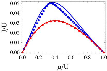
Figure 1: (Color online) First-order EPLT results (30) (solid) compared with GMFT results (34) (dots) for 3D cubic lattice when the driving parameter $A/(\hbar\omega)$ equals to $1$ (red) and $2.2$ (blue), respectively.

.

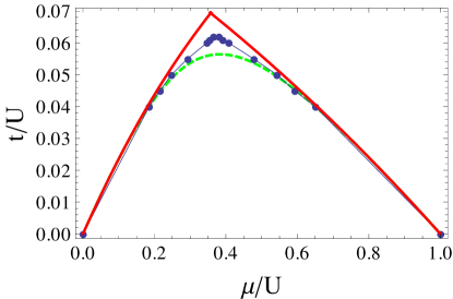
Figure 2: (Color online) Phase boundary of a 2D square lattice for $J_{0}\left(A/(\hbar\omega)\right)=0.4$: third-order strong-coupling expansion result according to (36), (37) (red solid line), QMC result in the thermodynamic limit (blue line dot), and second-order EPLT result (35) (green dashed line).

.

III.3 Higher Order and Numerical Results

Now we strive after obtaining more accurate results for the quantum phase boundary. At first, we consider EPLT in second hopping order, where the condition for the MI-SF phase transition reads

$$t=\frac{\tilde{\alpha}_{1}}{2\left(\tilde{\alpha}_{2}-\tilde{\alpha}_{1}^{2}\right)}+\frac{1}{2\left(\tilde{\alpha}_{2}-\tilde{\alpha}_{1}^{2}\right)}\sqrt{\tilde{\alpha}_{1}^{2}-4\left(\tilde{\alpha}_{2}-\tilde{\alpha}_{1}^{2}\right)}\,.$$ (35)

Here the abbreviations $\tilde{\alpha}_{1}=\alpha_{2}^{(1)}/\alpha_{2}^{(0)}$ and $\tilde{\alpha}_{2}=\alpha_{2}^{(2)}/\alpha_{2}^{(0)}$ follow from (24), (25) as well as (44)–(46) in Appendix B. In order to check how accurate the second-order EPLT result is, we compare it quantitatively for a 2D square lattice with two other approaches.

On the one hand we have applied the strong-coupling method of Ref. monien up to third order, yielding for $n=1$ a quantum phase boundary with the upper part

$$\mu_{1} = 1-2zt-t^{2}\left\{2z^{2}J_{0}^{2}(x)+z\left[\frac{3}{2}J_{0}^{2}(2x)-6J_{0}^{2}(x)\right]\right\}$$ (36)

$$-t^{3}\left\{6z^{3}J_{0}^{3}(x)+z^{2}\left[6J_{0}(2x)J_{0}^{2}(x)-24J_{0}^{2}(x)\phantom{\frac{3}{2}}\right.\right.$$

$$\left.\left.-\frac{3}{2}J_{0}^{2}(2x)\right]+z\left[18-6J_{0}(2x)\phantom{\frac{3}{2}}\right]\right\}$$

and the lower part

$$\mu_{2} = tz+t^{2}J_{0}^{2}(x)(2z^{2}-6z)$$ (37)

$$+t^{3}J_{0}^{2}(x)(6z^{3}-18z^{2}+12z)\,,$$

where we have introduced for brevity the dimensionless driving parameter $x=A/(\hbar\omega)$ and the coordination number $z=4$. Note that the second-order strong-coupling results (36) and (37) can also be recovered from second-order EPLT by solving the quantum phase boundary $t=t(\mu)$ in (35) for $\mu=\mu(t)$ up to second hopping order. This agreement order by order in the hopping expansion is insofar surprising as the strong-coupling method yields reliable results for low dimensions, whereas EPLT has shown to be most accurate for high dimensions pelster1 .

In addition we have obtained high-precision QMC results from developing an algorithm on the basis of a stochastic series expansion sse1 ; sse2 ; qmc1 ; qmc2 ; qmc3 . In order to get the high accuracy quantum phase diagram in the thermodynamic limit from QMC, we performed a finite-size scaling with the lattice sizes $N=8\times 8$, $10\times 10$, and $12\times 12$ at the temperature $T=U/(20N)$. From Fig. 2, we observe that the second-order EPLT result deviates not more than $6\%$ error from the QMC result in the considered range $0<A/(\hbar\omega)<x_{1}\approx 2.4$ of driving amplitudes. Thus, our second-order EPLT result is sufficiently accurate for studying quantitatively the effect of the periodic driving upon the quantum phase transition. Furthermore, we also read off from Fig. 2 that the QMC result lies between the third-order strong-coupling result and the second-order EPLT result. This suggests to evaluate both analytical methods to even higher hopping orders, for instance, by applying the process-chain approach martin3 . The true quantum phase boundary should then lie between the upper boundary provided by the strong-coupling method and the lower boundary from the EPLT method. This hypothesis cannot directly be tested for a 3D lattice system as it is quite hard to get a satisfying quantum phase diagram from QMC. However, as EPLT is more accurate for higher-dimensional systems pelster1 , it is suggestive that the error will even be smaller for a 3D cubic lattice.

Now we use our second-order EPLT result in order to analyze the critical points of the Mott lobes in more detail. Figure 3 shows the EPLT predictions for the relative critical hopping $\Delta t_{c}=t_{c}(A)/t_{c}(A=0)$ and the relative critical chemical potential $\Delta\mu_{c}=\left[\mu_{c}(A)-(n-1)U\right]/$ $\left[\mu_{c}(A=0)-(n-1)U\right]$ at the tip of different Mott lobes as a function of the driving amplitude $A$. From Fig. 3 a) we read off at first that a larger driving leads to an increase of the Mott lobe. Thus, similar to the shaken optical lattice martin1 , the periodic modulation of the s-wave scattering length provides a control knob to tune the quantum phase transition from Mott insulator to superfluid. Furthermore, it turns out that the effect of periodic driving upon the critical hopping at the lobe tip is slightly larger in $3$D than in $2$D systems, i.e. the driving effect is sensitive to the coordination number $z$. This can be intuitively understood from the hopping term in the effective Hamiltonian (20), which contains the Bessel function $J_{0}$ with the nearest neighbor particle difference as its argument. Generally speaking, higher-order hopping processes have a larger driving effect as they have a larger probability to involve a larger nearest neighbor particle difference, and there are more possible higher order hopping processes in higher dimensional systems. In addition, we find from Fig. 3 a) that the driving effect is quite small with respect to the filling number $n$ as all Mott lobes in both $2$D and $3$D lattices increase almost in the same way for a fixed driving amplitude. Also this observation is explained by the fact that the effective Hamiltonian (20) depends on the nearest neighbor particle number difference rather than on the respective particle number on each site.

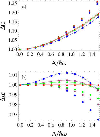
Figure 3: (Color online) Relative critical a) hopping $\Delta t_{c}=t_{c}(A)/t_{c}(A=0)$ and b) chemical potential $\Delta\mu_{c}=\left[\mu_{c}(A)-(n-1)U\right]/$ $\left[\mu_{c}(A=0)-(n-1)U\right]$ from second-order EPLT as a function of driving parameter $A/(\hbar\omega)$ for a 3D cubic lattice at tip of Mott lobes with $n=1$ (blue dot), $n=2$ (brown square dot), $n=3$ (green diamond dot), and $n=100$ (red triangular dot) as well as for a 2D square lattice (dots with lines).

We can also analyze the driving effect upon the critical chemical potential, which is depicted in Fig. 3 b). At first glance we observe that the critical chemical potential behaves differently in a $2$D square and a $3$D cubic lattice. It decreases monotonously in $3$D with increasing driving amplitude, but in 2D it reveals a nonmonotonous behavior and increases initially before it also finally decreases. Furthermore, we read off that the critical chemical potential changes only slightly with the driving amplitude $A$ and the filling number $n$. Up to the driving $A/(\hbar\omega)=1$ the critical potential changes less than one per cent, whereas for a huge filling number $n=100$ it almost does not change at all.

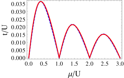
Figure 4: (Color online) Quantum phase diagram of the effective model (20) (red solid line) and the new effective model (38) (dashed blue line) with the driven parameter $A/(\hbar\omega)=1$ for a $3$D cubic lattice.

IV Effective Bose-Hubbard Model

In the previous section we have found that the critical hopping is uniformly renormalized according to Fig. 3 a) irrespective of the Mott lobe number $n$, whereas the critical chemical nearly does not change according to Fig. 3 b). This motivates to investigate in this section whether the whole quantum phase boundary for the effective Hamiltonian (20) stems approximately from the usual Bose-Hubbard Hamiltonian

$$\hat{H}=-t\lambda(x)\sum_{<ij>}\hat{a}_{i}^{{\dagger}}\hat{a}_{j}+\sum_{i}\frac{U}{2}\hat{n}_{i}(\hat{n}_{i}-1)-\sum_{i}\mu\hat{n}_{i}\,.$$ (38)

Here $\lambda(x)$ denotes a suitable rescaling of the hopping with the dimensionless driving parameter $x=A/(\hbar\omega)$ such that all Mott lobes coincide approximately. From Fig. 3 a), we determine via a Taylor expansion for $n=1$ the fit function

$$\lambda(x)=1+ax+bx^{2}+cx^{3}+dx^{4}+\ldots\,,$$ (39)

with $a=-0.0045$, $b=0.1356$, $c=0.0366$, $d=0.0129$ for a $3$D cubic lattice, while we have $a=-0.0018$, $b=0.1212$, $c=0.0561$, $d=0.0178$ for a $2$D square lattice. Figure 4 compares the resulting quantum phase diagram for the new effective model (38) with the original effective model (20). We read off that not only the critical point but also the complete quantum phase diagram is perfectly reproduced by the Bose-Hubbard model (38) with the fit function (39) in a $3$D cubic lattice. The same can also be observed in a $2$D square lattice provided the driving amplitude is not too large.

Furthermore, we have also used QMC simulations in order to investigate whether both models (20) and (38) also have the same properties in the superfluid phase. To this end we have calculated both the superfluid density $\rho_{s}=\langle W^{2}/2\beta t\rangle$ in terms of the winding number $W$ following Ref. winding and the difference between the total density and the density in Mott-I, i.e. $\Delta\rho=\mathop{\sum}_{i}\langle n_{i}\rangle/N-1$, as a function of the chemical potential. Figure 5 compares both quantities for the models (20) and (38). We read off that they perfectly agree near the quantum phase boundary, but farther away they slightly differ due to larger density fluctuations.

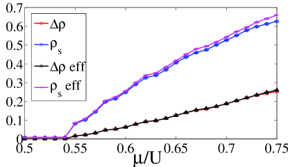
Figure 5: (Color online) Total density difference and superfluid density of the original model (20) and the effective model (38) for $t/U=0.05$, $A/(\hbar\omega)=0.4$, $N=8\times 8$, and $T=U/(20N)$ in $2$D square lattice.

V conclusion

We have applied the Floquet theory in order to analyze the effect of a periodic modulation of the s-wave scattering length upon the quantum phase diagram of bosons in an optical lattice. At first we have obtained a time-independent effective Hamiltonian for large enough driving frequencies. Then we used GMFT, EPLT, strong-coupling method, and QMC simulations in order to determine quantitatively how the different Mott lobes change with the driving amplitude. In particular, we have found that the time-independent effective model can be well described even by the usual Bose-Hubbard model provided that the hopping is rescaled appropriately with the driving amplitude. Thus, a period driving of the interaction allows to tune dynamically the hopping within an optical lattice. Furthermore, these findings corroborate the hypothesis that the Bose-Hubbard model with a periodically driven s-wave scattering length and the usual Bose-Hubbard model belong to the same universality class from the point of view of critical phenomena zinn-justin ; kleinert and, thus, should have the same critical exponents Fisher:PRB89 ; sachdev ; crit1 .

Appendix A Break Down of Factorization Rule

The perturbative coefficients $\alpha_{2p}^{(n)}$ in Eq. (23) follow from applying Rayleigh-Schrödinger perturbation theory by using a suitable diagrammatic representation pelster1 ; tao . By denoting the creation (annihilation) operator with an arrow line pointing into (out of) the site, each perturbative contribution of $\alpha_{2p}^{(n)}$ can be sketched as an arrow-line diagram, which is composed of $n$ oriented internal lines connecting the vertices and two external arrow lines. The vertices in the diagram correspond to the respective lattice sites, oriented internal lines stand for the hopping process between sites, and the two external arrow lines are representing creation and annihilation operators, respectively. To make this clearer, let us consider the simplest example of the coefficient $\alpha_{2}^{(1)}$, which has the following diagrammatic representation:

$$\alpha_{2}^{(1)}=\raisebox{-1.42271pt}{\includegraphics[width=85.35826pt]{figure6.eps}}\,.$$ (40)

In the usual Bose-Hubbard model, which we recover from the Hamiltonian (20) for vanishing driving, i.e. $A=0$, such a one-particle reducible diagram reduces into its one-particle irreducible contributions in formal analogy to the Feynman diagrams of quantum field theory zinn-justin ; kleinert . Thus, the diagrammatic representation (40) factorizes as follows:

$$\alpha_{2}^{(1)}=\raisebox{-0.85355pt}{\hskip 1.42271pt\includegraphics[width=28.45274pt]{figure7.eps}}\sum_{\langle i,j\rangle}t_{ij}\raisebox{-0.85355pt}{\hskip 1.42271pt\includegraphics[width=28.45274pt]{figure7.eps}}\,.$$ (41)

In the latter equation ’ ’ and ’$\sum_{\langle i,j\rangle}t_{ij}$’ turn out to be independent, so it can be rewritten for nearest neighbor hopping according to

$$\alpha_{2}^{(1)}=zt\left(\raisebox{-0.85355pt}{\hskip 1.42271pt\includegraphics[width=28.45274pt]{figure7.eps}}\right)^{2}\,.$$ (42)

For our effective Hamiltonian (20), however, the coefficient $\alpha_{2}^{(1)}$ results in

$$\alpha_{2}^{(1)}=\raisebox{-0.85355pt}{\hskip 1.42271pt\includegraphics[width=28.45274pt]{figure7.eps}}\sum_{\langle i,j\rangle}t_{ij}J_{0}\left(\frac{A}{\hbar\omega}\left(\hat{n}_{i}-\hat{n}_{j}\right)\right)\raisebox{-0.85355pt}{\hskip 1.42271pt\includegraphics[width=28.45274pt]{figure7.eps}}\,,$$ (43)

where the conditional hopping ’$\sum_{\langle i,j\rangle}t_{ij}J_{0}\left(\frac{A}{\hbar\omega}\left(\hat{n}_{i}-\hat{n}_{j}\right)\right)$’ depends on the occupation numbers of the neighboring sites, thus it is related to the diagrams ’ ’ which appear in front and thereafter. As a result, all three diagrammatic parts in equation (43) represent together one entity rather than three independent ones, thus yielding a break down of the factorization rule. This has the immediate consequence that one-particle reducible diagrams for non-vanishing driving will not vanish in the effective potential in any hopping order.

Appendix B Second Hopping Order

Due to the break down of the factorization rule the calculation of coefficients in Eq. (23) in higher hopping orders turns out to be much more elaborate. For instance, the dependence of the second-order coefficient $\alpha_{2}^{(2)}$ on the coordination number $z$ decomposes according to

$$\alpha_{2}^{(2)}=z(z-1)\alpha_{21}^{(2)}+z\alpha_{22}^{(2)}\,.$$ (44)

The first contribution reads

$$\alpha_{21}^{(2)} = \left[\frac{n}{f\left(n\right)-f\left(n-1\right)}+\frac{n+1}{f\left(n\right)-f\left(n+1\right)}\right]^{3}$$

$$+\left[J_{0}\left(\frac{A}{\hbar\omega}\right)+3\right]\left[J_{0}\left(\frac{A}{\hbar\omega}\right)-1\right]$$

$$\times\left\{\frac{n\left(n+1\right)^{2}}{\left[f(n)-f(n-1)\right]\left[f(n)-f(n+1)\right]^{2}}\right.$$

$$\left.+\frac{n^{2}\left(n+1\right)}{\left[f(n)-f(n-1)\right]^{2}\left[f(n)-f(n+1)\right]}\right\}$$

whereas the second term turns out to be

$$\alpha_{22}^{(2)} = \frac{n^{3}}{\left[f(n)-f(n-1)\right]^{3}}+\frac{\left(n+1\right)^{3}}{\left[f(n)-f(n+1)\right]^{3}}-\frac{(n-1)n(n+1)J_{0}^{2}\left(\frac{2A}{\hbar\omega}\right)}{\left[f(n)-f(n-1)\right]^{2}\left[f(n+1)+f(n-2)-2f(n)\right]}$$ (46)

$$+\frac{(n-1)n(n+1)J_{0}^{2}\left(\frac{A}{\hbar\omega}\right)}{\left[f(n-1)-f(n)\right]\left[f(n-1)+f(n+1)-2f(n)\right]^{2}}-\frac{n(n+1)(n+2)J_{0}^{2}\left(\frac{A}{\hbar\omega}\right)}{\left[f(n)-f(n+1)\right]\left[f(n-1)+f(n+1)-2f(n)\right]^{2}}$$

$$-\frac{(n-1)n(n+1)J_{0}^{2}\left(\frac{A}{\hbar\omega}\right)}{\left[f(n+1)+f(n-2)-2f(n)\right]\left[f(n-1)+f(n+1)-2f(n)\right]^{2}}$$

$$+\frac{2n^{2}(n+1)\left[J_{0}^{2}\left(\frac{A}{\hbar\omega}\right)-J_{0}\left(\frac{A}{\hbar\omega}\right)\right]}{\left[f(n-1)-f(n)\right]^{2}\left[f(n-1)+f(n+1)-2f(n)\right]}$$

$$+\frac{2n(n+1)^{2}\left[J_{0}^{2}\left(\frac{A}{\hbar\omega}\right)-J_{0}\left(\frac{A}{\hbar\omega}\right)\right]}{\left[f(n)-f(n+1)\right]^{2}\left[f(n-1)+f(n+1)-2f(n)\right]}-\frac{n(n+1)(n+2)J_{0}^{2}\left(\frac{2A}{\hbar\omega}\right)}{\left[f(n)-f(n+1)\right]^{2}\left[f(n-1)+f(n+2)-2f(n)\right]}$$

$$-\frac{2(n-1)n(n+1)J_{0}\left(\frac{A}{\hbar\omega}\right)J_{0}\left(\frac{2A}{\hbar\omega}\right)}{\left[f(n-1)-f(n)\right]\left[f(n-2)+f(n+1)-2f(n)\right]\left[f(n-1)+f(n+1)-2f(n)\right]}$$

$$-\frac{n(n+1)(n+2)J_{0}^{2}\left(\frac{A}{\hbar\omega}\right)}{\left[f(n+1)+f(n-1)-2f(n)\right]^{2}\left[f(n-1)+f(n+2)-2f(n)\right]}$$

$$+\frac{2n(n+1)(n+2)J_{0}\left(\frac{A}{\hbar\omega}\right)J_{0}\left(\frac{2A}{\hbar\omega}\right)}{\left[f(n)-f(n+1)\right]\left[f(n+2)+f(n-1)-2f(n)\right]\left[f(n-1)+f(n+1)-2f(n)\right]}\,.$$

References

- (1) M. P. A. Fisher, P. B. Weichman, G. Grinstein, and D. S. Fisher, Phys. Rev. B 40, 546 (1989).
- (2) D. Jaksch, C. Bruder, J. I. Cirac, C. W. Gardiner, and P. Zoller, Phys. Rev. Lett. 81, 3108 (1998).
- (3) M. Greiner, O. Mandel, T. Esslinger, T. W. Hänsch, and I. Bloch, Nature 415, 39 (2002).
- (4) M. Lewenstein, A. Sanpera, V. Ahufinger, B. Damski, A. S. De, and U. Sen, Adv. Phys. 56, 243 (2007).
- (5) I. Bloch, J. Dalibard, and W. Zwerger, Rev. Mod. Phys. 80, 885 (2008).
- (6) M. Lewenstein, A. Sanpera, and V. Ahufinger, Ultracold Atoms in Optical Lattices: Simulating Quantum Many-Body Systems (Oxford University Press, Oxford, 2012).
- (7) M. Inguscio and L. Fallani, Atomic Physics: Precise Measurements and Ultracold Matter, (Oxford University Press, Oxford, 2013).
- (8) I. Bloch, J. Dalibard and S. Nascimbène, Nature Phys. 8, 267 (2012).
- (9) I. Bloch, Nature Phys. 1, 23 (2005).
- (10) D. Jaksch and P. Zoller, Ann. Phys. (New York) 315, 52 (2005).
- (11) R. Feyman, Int. J. Theor. Phys. 21, 467 (1982).
- (12) A. Eckardt, C. Weiss, and M. Holthaus, Phys. Rev. Lett. 95, 260404 (2005).
- (13) H. Lignier, C. Sias, D. Ciampini, Y. Singh, A. Zenesini, O. Morsch, and E. Arimondo, Phys. Rev. Lett. 99, 220403 (2007).
- (14) E. Kierig, U. Schnorrberger, A. Schietinger, J. Tomkovic, and M. K. Oberthaler, Phys. Rev. Lett. 100, 190405 (2008).
- (15) A. Zenesini, H. Lignier, D. Ciampini, O. Morsch, and E. Arimondo, Phys. Rev. Lett. 102, 100403 (2009).
- (16) J. Struck, C. Ölschläger, R. Le Targat, P. Soltan-Panahi, A. Eckardt, M. Lewenstein, P. Windpassinger, and K. Sengstock, Science 333, 996 (2011).
- (17) J. Struck, C. Ölschläger, M. Weinberg, P. Hauke, J. Simonet, A. Eckardt, M. Lewenstein, K. Sengstock, P. Windpassinger, Phys. Rev. Lett. 108, 225304 (2012).
- (18) P. Hauke, O. Tieleman, A. Celi, C. Ölschläger, J. Simonet, J. Struck, M. Weinberg, P. Windpassinger, K. Sengstock, M. Lewenstein, and A. Eckardt, Phys. Rev. Lett. 109, 145301 (2012).
- (19) J. Struck, M. Weinberg, C. Ölschläger, P. Windpassinger, J. Simonet, K. Sengstock, R. Höppner, P. Hauke, A. Eckardt, M. Lewenstein, and L. Mathey, Nature Phys. 9, 738 (2013).
- (20) M. Aidelsburger, M. Atala, M. Lohse, J. T. Barreiro, B. Paredes, and I. Bloch, Phys. Rev. Lett. 111, 185301 (2013).
- (21) H. Miyake, G. A. Siviloglou, C. J. Kennedy, W. C. Burton, and W. Ketterle, Phys. Rev. Lett. 111, 185302 (2013).
- (22) E. R. F. Ramos, E. A. L. Henn, J. A. Seman, M. A. Caracanhas, K. M. F. Magalhaes, K. Helmerson, V. I. Yukalov, and V. S. Bagnato, Phys. Rev. A 78, 063412 (2008).
- (23) S. E. Pollack, D. Dries, R. G. Hulet, K. M. F. Magalhaes, E. A. L. Henn, E. R. F. Ramos, M. A. Caracanhas, and V. S. Bagnato, Phys. Rev. A 81, 053627 (2010).
- (24) S. E. Pollack, D. Dries, M. Junker, Y. P. Chen, T. A. Corcovilos, and R. G. Hulet, Phys. Rev. Lett. 102, 090402 (2009).
- (25) I. Vidanovic, A. Balaz, H. Al-Jibbouri, and A. Pelster, Phys. Rev. A 84, 013618 (2011).
- (26) A. Rapp, X. Deng, and L. Santos, Phys. Rev. Lett. 109, 203005 (2012).
- (27) J. Hubbard, Proc. Roy. Soc. A 276, 238 (1963).
- (28) J. E. Hirsch, Physica C 158, 326 (1989).
- (29) J. E. Hirsch and F. Marsiglio, Phys. Rev. 39, 11515 (1989).
- (30) L. Arrachea and A. A. Aligia, Phys. Rev. Lett. 73, 2240 (1994).
- (31) C. Vitoriano and M. D. Coutinho-Filho, Phys. Rev. Lett. 102, 146404 (2009).
- (32) R. Ma, M. E. Tai, P. M. Preiss, W. S. Bakr, J. Simon, and M. Greiner, Phys. Rev. Lett. 107, 095301 (2011).
- (33) T. Keilmann, S. Lanzmich, I. McCulloch, and M. Roncaglia, Nature Comm. 2, 361 (2011).
- (34) H. Sambe, Phys. Rev. A 7, 2203 (1973).
- (35) E. Arimondo, D. Ciampini, A. Eckardt, M. Holthaus, and O. Morsch, Adv. At. Mol. Opt. Phys. 61, 515 (2012).
- (36) A. Eckardt and M. Holthaus, Phys. Rev. Lett. 101, 245302 (2008).
- (37) F. E. A. dos Santos and A. Pelster, Phys. Rev. A 79, 013614 (2009).
- (38) B. Bradlyn, F. E. A. dos Santos, and A. Pelster, Phys. Rev. A 79, 013615 (2009).
- (39) T. D. Grass, F.E.A. dos Santos, and A. Pelster, Phys. Rev. A 84, 013613 (2011).
- (40) T. Wang, X.-F. Zhang, S. Eggert, and A. Pelster: Phys. Rev. A 87, 063615 (2013).
- (41) M. Ohliger and A. Pelster, World J. Cond. Mat. Phys. 3, 125 (2013).
- (42) M. Mobarak and A. Pelster, Laser Phys. Lett. 10, 115501 (2013).
- (43) N. Teichmann, D. Hinrichs, M. Holthaus, and A. Eckardt Phys. Rev. B 79, 224515 (2009).
- (44) B. Capogrosso-Sansone, N. V. Prokof’ev, and B. V. Svistunov, Phys. Rev. B 75, 134302 (2007).
- (45) D. S. Rokhsar and B. G. Kotliar, Phys. Rev. B 44, 10328 (1991).
- (46) W. Krauth, M. Caffarel, and J.-P. Bouchaud, Phys. Rev. B 45, 3137 (1992).
- (47) W. Zwerger, J. Opt. B: Quantum Semiclass. Opt. 5, S9 (2003).
- (48) P. Buonsante and V. Penna, J. Phys. A: Math. Theor. 41, 175301 (2008).
- (49) C. Trefzger, C. Menotti, B. Capogrosso-Sansone, and M. Lewenstein, J. Phys. B: At. Mol. Opt. Phys. 44, 193001 (2011).
- (50) D. S. Lühmann, Phys. Rev. A 87, 043619 (2013).
- (51) J. K. Freericks and H. Monien, Phys. Rev. B 53, 2691 (1996).
- (52) A. W. Sandvik, Phys. Rev. B 59, R14157 (1999).
- (53) O. F. Syljuåsen and A. W. Sandvik, Phys. Rev. E 66, 046701 (2002).
- (54) X.-F. Zhang, Y.-C. Wen, and S. Eggert, Phys. Rev. B 82, 220501(R) (2010).
- (55) X.-F. Zhang, R. Dillenschneider, Y. Yu, and S. Eggert, Phys. Rev. B 84, 174515 (2011).
- (56) X.-F. Zhang, Q. Sun, Y.-C. Wen, W.-M. Liu, S. Eggert, and A.-C. Ji, Phys. Rev. Lett. 110, 090402 (2013).
- (57) E. L. Pollock and D. M. Ceperley, Phys. Rev. B 36, 8343 (1987).
- (58) J. Zinn-Justin, Quantum Field Theory and Critical Phenomena, 4th ed. (Oxford University Press, Oxford, 2002).
- (59) H. Kleinert and V. Schulte-Frohlinde, Critical Properties of Theories (World Scientific, Singapore, 2001).
- (60) S. Sachdev, Quantum phase transitions, 2nd ed. (Cambridge University Press, Cambridge, 2011).
- (61) D. Hinrichs, A. Pelster, and M. Holthaus, Appl. Phys. B 113, 57 (2013).