Role of functionality in two-component signal transduction: A stochastic study

Abstract

We present a stochastic formalism for signal transduction processes in a bacterial two-component system. Using elementary mass action kinetics, the proposed model takes care of signal transduction in terms of phosphotransfer mechanism between the cognate partners of a two-component system, viz, the sensor kinase and the response regulator. Based on the difference in functionality of the sensor kinase, the noisy phosphotransfer mechanism has been studied for monofunctional and bifunctional two component system using the formalism of linear noise approximation. Steady state analysis of both models quantifies different physically realizable quantities, e.g., variance, Fano factor (variance/mean), mutual information. The resultant data reveals that both systems reliably transfer information of extra-cellular environment under low external stimulus and at high kinase and phosphatase regime. We extend our analysis further by studying the role of two-component system in downstream gene regulation.

I Introduction

In response to the changes made in the extra-cellular environment, living systems adapt themselves by coordinated regulation of intracellular machinery composed of several interacting components McAdams and Shapiro (1995); Tyson et al. (2003); Alon (2007). In bacterial kingdom, such adaptation is achieved by a group of highly specialized motifs, commonly known as two-component system (TCS) West and Stock (2001); Laub and Goulian (2007); Kenney (2010). Comprised of membrane bound sensor kinase and cytoplasmic response regulator, TCS detects changes made in the environment and, in response, controls expression and/or repression of one or several downstream genes (target genes other than operon). In presence of an external stimulus, autophosphorylation takes place in the conserved histidine residue of the sensor kinase. The phosphate group is then transferred to its cognate partner, the response regulator, containing conserved aspartate domain. When phosphorylated, the response regulator regulates one or several downstream genes, as well as its own operon. For example, in M. tuberculosis, the response regulator MprA gets phosphorylated by its cognate sensor MprB in presence of the signal and exerts a positive feedback on its own operon mprAB Tiwari et al. (2010). In addition to being the source of phosphate group, sensor kinase sometimes can dephosphorylate phosphate group from a response regulator by acting as phosphatase. This combined kinase and phosphatase activity of the sensor kinase makes the TCS bifunctional Hsing et al. (1998); Laub and Goulian (2007); Kenney (2010); Goldberg et al. (2010). Due to the opposing (kinase and phosphatase) effect of sensor kinase on response regulator, bifunctional systems have been placed in a broad category of functional motifs known as paradoxical components Hart et al. (2012); Hart and Alon (2013). In certain TCS, role of sensor as a phosphatase is absent, and the job of dephosphorylation is done by an auxiliary protein (phosphatase), thus making the TCS monofunctional Laub and Goulian (2007); Kenney (2010).

Depending on the nature of extra-cellular stimulus, a single bacterium may utilize different types of TCS with highly specific functionality to transduce the changes made in the surroundings. To sense and adapt appropriately, a single bacterium may contain both monofunctional and bifunctional TCS Laub and Goulian (2007); Kenney (2010). For example, E. coli chemotaxis system has CheA/CheY TCS that responds to change in the chemical gradient in the surrounding where the sensor kinase CheA is monofunctional in nature (acts as kinase only) and role of phosphatase is played by CheZ which is not a part of the TCS. On the other hand, EnvZ/OmpR TCS in E. coli responds to change in the osmolarity of the environment where sensor kinase EnvZ plays a bifunctional role (acts as kinase as well as phosphatase). One of the advantages of a bifunctional system over a monofunctional one is that it takes care of input-output robustness Shinar et al. (2007). Due to its architecture, the output level of the phosphorylated response regulator in a bifunctional system depends only on the input stimulus and is independent of other system components. On the other hand, such a robustness criterion does not remain valid in a monofunctional system. Thus, in the latter case, in addition to the input stimulus, the output level depends also on the level of phosphatase which acts on the phosphorylated response regulator.

When the aforesaid signal transduction processes are considered within the single cell scenario, role of fluctuations, cellular and/or extra-cellular, cannot be ruled out. Whether external or internal, such fluctuations not only affect the gene expression mechanism within a cell but also control the signal transduction processes involving post-translational modifications that are taking place within a noisy environment. With the advancement of experimental techniques that employ single cell measurement, it is now possible to quantify different physically realizable quantities like variance, Fano factor (variance/mean), etc., of different cellular componentsPaulsson (2004); Rosenfeld et al. (2005); Zaslaver et al. (2006); Kaern et al. (2005); Silva-Rocha and de Lorenzo (2010); Eldar and Elowitz (2010); Balázsi et al. (2011); Munsky et al. (2012). In this light, it is thus worthwhile to develop a stochastic formalism to study signal transduction processes in bacterial TCS keeping in mind the difference in functionality of the sensor kinase. Although deterministic modeling of bacterial signal transduction machinery is known in the literature Alves and Savageau (2003); Bandyopadhyay and Banik (2012); Shinar et al. (2007); Igoshin et al. (2008); Miyashiro and Goulian (2008); Tiwari et al. (2010), few attempts have been made to study the same using a stochastic framework. In this connection, it is important to mention the theoretical modeling of bacterial two component system where stochastic kinetics has been used to study different phenotypic response (graded and all-or-none) Kierzek et al. (2010); Hoyle et al. (2012). In the present work, however, we have developed a mathematical formalism to study signal transduction processes in generic bacterial TCS. While developing the model, we have taken into account only the post-translational modification in terms of phosphorylation-dephosphorylation kinetics as the timescale of the phosphotransfer kinetics is faster than the synthesis and/or degradation timescale of the system components Alves and Savageau (2003). As mentioned earlier, the main role of TCS is to transmit the information of changes in the extra-cellular environment reliably within the cell. In the proposed stochastic study, we compare information processing in TCS with the monofunctional and the bifunctional property of sensor kinase. Combining both theoretical and numerical approaches, we show that for a fixed level of fluctuations due to stimulus, bifunctional TCS carries out a more reliable signal processing compared to monofunctional TCS.

The rest of the paper is organized as follows. In the next section, we develop the mathematical model to study signal transduction mechanism in monofunctional and in bifunctional system. Results of the model are discussed in Sec. III and the paper is concluded in Sec. IV.

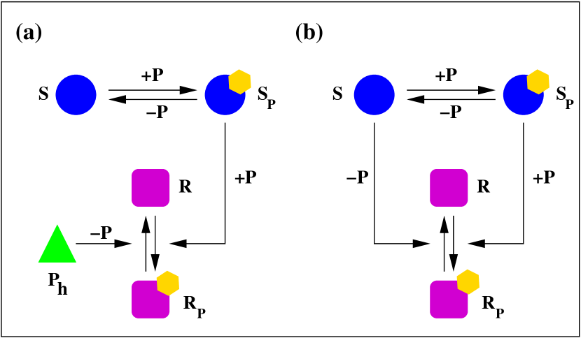
Figure 1: (color online) Schematic diagram of phosphotransfer motif in (a) monofunctional and (b) bifunctional two component system. $S$ and $S_{p}$ stand for unphosphorylated and phosphorylated form of sensor kinase, respectively. Similarly, $R$ and $R_{p}$ stand for unphosphorylated and phosphorylated form of response regulator, respectively. $P_{h}$ stands for phosphatase. $\pm P$ stand for addition/removal of the phosphate group (shown by orange hexagon). Note that in monofunctional system, sensor kinase acts as a source of phosphate group whereas, in bifunctional system, it acts both as source and sink for the phosphate group.

II The model

Following phosphotransfer kinetics depicted in Fig. (1) for both monofunctional and bifunctional systems, we have developed a mathematical model for noisy signal transduction in the present communication. In presence of an external inducer $I$, sensor kinase $S$ gets phosphorylated at the conserved histidine residue to form $S_{p}$. Phosphorylated sensor then transfers the phosphate group to its cognate response regulator $R$, forming $R_{p}$. It is important to note that the above mentioned kinetics is common for both monofunctional and bifunctional systems. When it comes to removal of the phosphate group (dephosphorylation) from the response regulator, the two systems (monofunctional and bifunctional) behave differently. In the monofunctional system, the phosphate group from $R_{p}$ is removed by a phosphatase $P_{h}$ whereas, in the bifunctional one, the phosphate group is removed by the unphosphorylated sensor $S$ itself. Thus, in monofunctional system, the sensor acts as a source of phosphate group and, in bifunctional system, the same acts as a sink in addition to being a source of the phosphate group. Considering the aforesaid interactions, the minimal kinetic steps for the phosphotransfer motif can be written as

$$\overset{k_{sI}}{\longrightarrow}I \overset{k_{dI}}{\longrightarrow} \varnothing,$$ (1a)

$$S \overset{k_{p}I}{\underset{k_{dp}}{\rightleftharpoons}} S_{p},$$ (1b)

$$S_{p}+R \overset{k_{k}}{\longrightarrow} S+R_{p},$$ (1c)

$$P_{h}+R_{p} \overset{k_{pm}}{\longrightarrow} P_{h}+R,$$ (1d)

$$\overset{k_{sP_{h}}}{\longrightarrow}P_{h} \overset{k_{dP_{h}}}{\longrightarrow} \varnothing,$$ (1e)

$$S+R_{p} \overset{k_{pb}}{\longrightarrow} S+R.$$ (1f)

In the above kinetic steps, Eq. (1a) refers to the synthesis and degradation of the external inducer $I$. Eq. (1b) takes care of autophosphorylation and dephosphorylation of the sensor kinase. While modeling the autophosphorylation reaction, we have considered the signal $I$ as a catalyst which helps to convert the sensor $S$ to its phosphorylated form ($S_{p}$). However, theoretical formalism developed earlier considered a more general framework for stochastic signaling through enzymatic futile cycles Samoilov et al. (2005). Eq. (1c) considers the kinase reaction and Eq. (1d) considers the phosphatase activity of $P_{h}$ towards $R_{p}$. It is important to mention that while writing the kinase and the phosphatase kinetics, we have considered second order bi-molecular reaction scheme, although these reaction kinetics are generally written using Michaelis-Menten type kinetics in the existing literature Alves and Savageau (2003); Bandyopadhyay and Banik (2012); Igoshin et al. (2008); Miyashiro and Goulian (2008); Tiwari et al. (2010). One of the advantages of using Michaelis-Menten kinetics is that it generates ultrasensitive switch in a system Goldbeter and Koshland (1981, 1982); Tănase-Nicola et al. (2006); Kierzek et al. (2010); Tiwari et al. (2010) provided the network architecture generates substantial nonlinearity. However, the reason behind using the second order bi-molecular reaction scheme in the present work is that it makes our analytical calculation tractable as shown in Sec. IIA and Sec. IIB. Since the auxiliary protein $P_{h}$ behaves as an alternative source of phosphatase in the monofunctional system, it is worthwhile to consider its kinetics (synthesis and degradation) in the model. To this end, production and degradation of the phosphatase $P_{h}$ has been taken care of by Eq. (1e). Finally, Eq. (1f) is due to the phosphatase activity of $S$ towards $R_{p}$. Note that Eqs. (1a-1c) are common for both monofunctional and bifunctional systems. Eqs. (1d-1e) are exclusive for the monofunctional system and Eq. (1f) is solely for the bifunctional system. While writing the kinetic steps, we have mostly considered the post-translational modification for sensor and response regulator. As mentioned earlier, we do not consider synthesis and degradation of the system components ($S$ and $R$) in the proposed model which keeps the total amount of sensor and response regulator constant, i.e., $S+S_{p}=S_{T}$ and $R+R_{p}=R_{T}$.

To understand the role of fluctuations prevalent due to the external inducer $I$ and the intrinsic cellular noise affecting the phosphotransfer mechanism, we adopt Langevin approach to define different physical quantities. Langevin approach within the purview of linear noise approximation is a valid approach provided fluctuations in the input signal are very small so that one can linearize the resultant noise in the Langevin equation Paulsson (2004); Simpson et al. (2004); Shibata and Fujimoto (2005); Tănase-Nicola et al. (2006). Such linearization also remains valid when the coarse grained (steady state) time scale is longer than the birth-death rate of system components. In addition, a large copy number of system components makes the approximation valid. Since in TCS, copy numbers of $S$ and $R$ are large, one can adopt Langevin formalism to understand the stochastic signal transduction mechanism. Thus, the Langevin equation associated with the inducer kinetics is given by,

$$\frac{dI}{dt}=k_{sI}-k_{dI}I+\xi_{I},$$ (2)

where

$$\langle\xi_{I}(t)\rangle=0,\;\langle\xi_{I}(t)\xi_{I}(t+\tau)\rangle=2k_{dI}\langle I\rangle\delta(\tau),$$ (3)

with $\langle I\rangle$ being the mean inducer level at steady state. It is important to note that Eqs. (2-3) are common for both monofunctional and bifunctional systems.

II.1 Monofunctional system

Considering the kinetic steps given by Eqs. (1b-1e) and fluctuations associated with them, the Langevin equations for $S_{p}$, $R_{p}$ and $P_{h}$ for the monofunctional system can be written as

$$\frac{dS_{p}}{dt} = k_{p}(S_{T}-S_{p})I-k_{dp}S_{p}$$ (4a)

$$-k_{k}S_{p}(R_{T}-R_{p})+\xi_{S_{p}},$$

$$\frac{dR_{p}}{dt} = k_{k}S_{p}(R_{T}-R_{p})-k_{pm}P_{h}R_{p}+\xi_{R_{p}},$$ (4b)

$$\frac{dP_{h}}{dt} = k_{sP_{h}}-k_{dP_{h}}P_{h}+\xi_{P_{h}}.$$ (4c)

The additive noise terms $\xi_{S_{p}}$, $\xi_{R_{p}}$ and $\xi_{P_{h}}$ take care of fluctuations in the copy number of $S_{p}$, $R_{p}$ and $P_{h}$, respectively. Using the concept of linear noise approximation, the statistical properties of three fluctuating terms can be written as van Kampen (2005); Elf and Ehrenberg (2003); Mehta et al. (2008)

$$\langle\xi_{S_{p}}(t)\xi_{S_{p}}(t+\tau)\rangle_{m} = 2k_{p}[S_{T}-\langle S_{p}\rangle_{m}]\langle I\rangle\delta(\tau),$$ (5a)

$$\langle\xi_{R_{p}}(t)\xi_{R_{p}}(t+\tau)\rangle_{m} = 2k_{k}\langle S_{p}\rangle_{m}[R_{T}-\langle R_{p}\rangle_{m}]$$ (5b)

$$\times\delta(\tau),$$

$$\langle\xi_{P_{h}}(t)\xi_{P_{h}}(t+\tau)\rangle_{m} = 2k_{dP_{h}}\langle P_{h}\rangle\delta(\tau),$$ (5c)

with $\langle\xi_{S_{p}}(t)\rangle_{m}=\langle\xi_{R_{p}}(t)\rangle_{m}=\langle\xi_{P_{h}}(t)\rangle_{m}=0$. In the above equations, $\langle S_{p}\rangle_{m}$ and $\langle R_{p}\rangle_{m}$ stand for the mean values of $S_{p}$ and $R_{p}$ at the steady state, respectively. Here, $\langle\cdots\rangle_{m}$ has been used to designate ensemble average for a monofunctional system. Furthermore, we consider that the noise terms $\xi_{S_{p}}$ and $\xi_{R_{p}}$ are correlated Tănase-Nicola et al. (2006); Swain (2004)

$$\langle\xi_{S_{p}}(t)\xi_{R_{p}}(t+\tau)\rangle_{m}=-k_{k}\langle S_{p}\rangle_{m}[R_{T}-\langle R_{p}\rangle_{m}]\delta(\tau).$$ (5d)

Linearizing Eq. (2) and Eqs. (4a-4c) around the mean value at steady state, i.e., $I=\langle I\rangle+\delta I$, $S_{p}=\langle S_{p}\rangle_{m}+\delta S_{p}$, $R_{p}=\langle R_{p}\rangle_{m}+\delta R_{p}$ and $P_{h}=\langle P_{h}\rangle+\delta P_{h}$, we have

$$\frac{d}{dt}\left(\begin{array}[]{c}\delta I\\ \delta S_{p}\\ \delta R_{p}\\ \delta P_{h}\end{array}\right) = \left(\begin{array}[]{cccc}-J_{II}&J_{IS_{p}}&J_{IR_{p}}&J_{IP_{h}}\\ J_{S_{p}I}&-J_{S_{p}S_{p}}&J_{S_{p}R_{p}}&J_{S_{p}P_{h}}\\ J_{R_{p}I}&J_{R_{p}S_{p}}&-J_{R_{p}R_{p}}&-J_{R_{p}P_{h}}\\ J_{P_{h}I}&J_{P_{h}S_{p}}&J_{P_{h}R_{p}}&-J_{P_{h}P_{h}}\end{array}\right)$$ (23)

$$\times\left(\begin{array}[]{c}\delta I\\ \delta S_{p}\\ \delta R_{p}\\ \delta P_{h}\end{array}\right)+\left(\begin{array}[]{c}\xi_{I}\\ \xi_{S_{p}}\\ \xi_{R_{p}}\\ \xi_{P_{h}}\end{array}\right),$$

with

$$J_{II}=k_{dI},J_{IS_{p}}=J_{IR_{p}}=J_{IP_{h}}=0,$$

$$J_{SpI}=k_{p}[S_{T}-\langle S_{p}\rangle_{m}],$$

$$J_{S_{p}S_{p}}=k_{p}\langle I\rangle+k_{dp}+k_{k}[R_{T}-\langle R_{p}\rangle_{m}],$$

$$J_{S_{p}R_{p}}=k_{k}\langle S_{p}\rangle_{m},J_{S_{p}P_{h}}=J_{R_{p}I}=0,$$

$$J_{R_{p}S_{p}}=k_{k}[R_{T}-\langle R_{p}\rangle_{m}],$$

$$J_{R_{p}R_{p}}=k_{k}\langle S_{p}\rangle_{m}+k_{pm}\langle P_{h}\rangle,J_{R_{p}P_{h}}=k_{pm}\langle R_{p}\rangle_{m},$$

$$J_{P_{h}I}=J_{P_{h}S_{p}}=J_{P_{h}R_{p}}=0.$$

Fourier transformation ($\delta\tilde{X}(\omega)=\int_{-\infty}^{+\infty}\delta X(t)\exp(-i\omega t)$ $dt$) of Eq. (23) gives

$$\left(\begin{array}[]{c}i\omega\delta\tilde{I}\\ i\omega\delta\tilde{S}_{p}\\ i\omega\delta\tilde{R}_{p}\\ i\omega\delta\tilde{P}_{h}\end{array}\right) = \left(\begin{array}[]{cccc}-J_{II}&J_{IS_{p}}&J_{IR_{p}}&J_{IP_{h}}\\ J_{S_{p}I}&-J_{S_{p}S_{p}}&J_{S_{p}R_{p}}&J_{S_{p}P_{h}}\\ J_{R_{p}I}&J_{R_{p}S_{p}}&-J_{R_{p}R_{p}}&-J_{R_{p}P_{h}}\\ J_{P_{h}I}&J_{P_{h}S_{p}}&J_{P_{h}R_{p}}&-J_{P_{h}P_{h}}\end{array}\right)$$ (41)

$$\times\left(\begin{array}[]{c}\delta\tilde{I}\\ \delta\tilde{S}_{p}\\ \delta\tilde{R}_{p}\\ \delta\tilde{P}_{h}\end{array}\right)+\left(\begin{array}[]{c}\tilde{\xi}_{I}\\ \tilde{\xi}_{S_{p}}\\ \tilde{\xi}_{R_{p}}\\ \tilde{\xi}_{P_{h}}\end{array}\right).$$

Solving Eq. (41) yields

$$(i\omega+J_{S_{p}S_{p}})\delta\tilde{S}_{p} = J_{S_{p}I}\delta\tilde{I}+J_{S_{p}R_{p}}\delta\tilde{R}_{p}+\tilde{\xi}_{S_{p}},$$

$$(i\omega+J_{R_{p}R_{p}})\delta\tilde{R}_{p} = J_{R_{p}S_{p}}\delta\tilde{S}_{p}-J_{R_{p}P_{h}}\delta\tilde{P}_{h}+\tilde{\xi}_{R_{p}},$$

$$(i\omega+J_{II})\delta\tilde{I} = \tilde{\xi}_{I},(i\omega+J_{P_{h}P_{h}})\delta\tilde{P}_{h}=\tilde{\xi}_{P_{h}},$$

which finally leads to the desired expression of $\delta\tilde{R}_{p}$ for the monofunctional system,

$$\delta\tilde{R}_{p} = \frac{J_{R_{p}S_{p}}J_{S_{p}I}\delta\tilde{I}}{(i\omega+J_{R_{p}R_{p}})(i\omega+J_{S_{p}S_{p}})-J_{R_{p}S_{p}}J_{S_{p}R_{p}}}$$ (42)

$$-\frac{[(i\omega+J_{S_{p}S_{p}})J_{R_{p}P_{h}}]\delta\tilde{P}_{h}}{(i\omega+J_{R_{p}R_{p}})(i\omega+J_{S_{p}S_{p}})-J_{R_{p}S_{p}}J_{S_{p}R_{p}}}$$

$$+\frac{(i\omega+J_{S_{p}S_{p}})\tilde{\xi}_{R_{p}}}{(i\omega+J_{R_{p}R_{p}})(i\omega+J_{S_{p}S_{p}})-J_{R_{p}S_{p}}J_{S_{p}R_{p}}}$$

$$+\frac{J_{R_{p}S_{p}}\tilde{\xi}_{S_{p}}}{(i\omega+J_{R_{p}R_{p}})(i\omega+J_{S_{p}S_{p}})-J_{R_{p}S_{p}}J_{S_{p}R_{p}}},$$

where

$$\delta\tilde{I}=\frac{\tilde{\xi}_{I}}{i\omega+J_{II}},\delta\tilde{P}_{h}=\frac{\tilde{\xi}_{P_{h}}}{i\omega+J_{P_{h}P_{h}}}.$$ (43)

In Eq. (42), the first term arises due to external inducer I. The second term is due to fluctuations in the phosphatase activity of $P_{h}$ on $R_{p}$. The third and fourth terms arise due to fluctuations in $R_{p}$ and $S_{p}$, respectively. Now, using the expression of $\delta\tilde{R}_{p}$ given in Eq. (42) and employing the properties of linear noise approximation given in Eqs. (5a-5d), we define the variance associated with $R_{p}$ for the monofunctional system,

$$\sigma^{2}_{R_{p}} = \frac{1}{2\pi}\int d\omega\left\langle\left|\delta\tilde{R}_{p}(\omega)\right|^{2}\right\rangle_{m},$$ (44)

$$= \frac{J^{2}_{R_{p}S_{p}}J^{2}_{S_{p}I}\langle I\rangle(\alpha_{m}+\beta_{m}+J_{II})}{\alpha_{m}\beta_{m}(\alpha_{m}+\beta_{m})(\alpha_{m}+J_{II})(\beta_{m}+J_{II})}$$

$$+\frac{J^{2}_{R_{p}P_{h}}\langle P_{h}\rangle}{\alpha_{m}\beta_{m}}$$

$$\times\frac{(\beta_{m}+J_{P_{h}P_{h}})J^{2}_{S_{p}S_{p}}+\alpha_{m}(\beta_{m}J_{P_{h}P_{h}}+J^{2}_{S_{p}S_{p}})}{(\alpha_{m}+\beta_{m})(\alpha_{m}+J_{P_{h}P_{h}})(\beta_{m}+J_{P_{h}P_{h}})}$$

$$+\frac{\gamma_{m}+k_{k}\langle S_{p}\rangle_{m}[R_{T}-\langle R_{p}\rangle_{m}](J^{2}_{S_{p}S_{p}}+\alpha_{m}\beta_{m})}{\alpha_{m}\beta_{m}(\alpha_{m}+\beta_{m})},$$

with

$$\alpha_{m} = \frac{1}{2}\left[(J_{S_{p}S_{p}}+J_{R_{p}R_{p}})\right.$$

$$\left.+\left\{(J_{S_{p}S_{p}}-J_{R_{p}R_{p}})^{2}+4J_{S_{p}R_{p}}J_{R_{p}S_{p}}\right\}^{1/2}\right],$$

$$\beta_{m} = \frac{1}{2}\left[(J_{S_{p}S_{p}}+J_{R_{p}R_{p}})\right.$$

$$\left.-\left\{(J_{S_{p}S_{p}}-J_{R_{p}R_{p}})^{2}+4J_{S_{p}R_{p}}J_{R_{p}S_{p}}\right\}^{1/2}\right],$$

$$\gamma_{m} = J^{2}_{R_{p}S_{p}}k_{p}(S_{T}-\langle S_{p}\rangle_{m})\langle I\rangle$$

$$-J_{R_{p}S_{p}}J_{S_{p}S_{p}}k_{k}\langle S_{p}\rangle_{m}(R_{T}-\langle R_{p}\rangle_{m}).$$

II.2 Bifunctional system

Considering the kinetic steps given by Eqs. (1b-1c,1f) and fluctuations associated with them, the Langevin equations for $S_{p}$ and $R_{p}$ for the bifunctional system can be written as

$$\frac{dS_{p}}{dt} = k_{p}(S_{T}-S_{p})I-k_{dp}S_{p}$$ (45a)

$$-k_{k}S_{p}(R_{T}-R_{p})+\xi_{S_{p}},$$

$$\frac{dR_{p}}{dt} = k_{k}S_{p}(R_{T}-R_{p})-k_{pb}R_{p}(S_{T}-S_{p})$$ (45b)

$$+\xi_{R_{p}}.$$

The additive noise terms $\xi_{S_{p}}$ and $\xi_{R_{p}}$ take care of fluctuations in the copy number of $S_{p}$ and $R_{p}$, respectively. The statistical properties of the two fluctuating terms are given by van Kampen (2005); Elf and Ehrenberg (2003); Mehta et al. (2008)

$$\langle\xi_{S_{p}}(t)\xi_{S_{p}}(t+\tau)\rangle_{b} = 2k_{p}[S_{T}-\langle S_{p}\rangle_{b}]\langle I\rangle\delta(\tau),$$ (46a)

$$\langle\xi_{R_{p}}(t)\xi_{R_{p}}(t+\tau)\rangle_{b} = 2k_{k}\langle S_{p}\rangle_{b}[R_{T}-\langle R_{p}\rangle_{b}]$$ (46b)

$$\times\delta(\tau),$$

with $\langle\xi_{S_{p}}(t)\rangle_{b}=\langle\xi_{R_{p}}(t)\rangle_{b}=0$. In the above equations, $\langle S_{p}\rangle_{b}$ and $\langle R_{p}\rangle_{b}$ stand for the mean values of $S_{p}$ and $R_{p}$ at the steady state, respectively. Here, $\langle\cdots\rangle_{b}$ has been used to designate ensemble average for a bifunctional system. As in monofunctional system, we consider the noise terms $\xi_{S_{p}}$ and $\xi_{R_{p}}$ to be correlated Tănase-Nicola et al. (2006); Swain (2004)

$$\langle\xi_{S_{p}}(t)\xi_{R_{p}}(t+\tau)\rangle_{b}=-k_{k}\langle S_{p}\rangle_{b}[R_{T}-\langle R_{p}\rangle_{b}]\delta(\tau).$$ (46c)

At this point it is important to note the difference between Eq. (4b) and Eq. (45b). In Eq. (4b), the loss term ($k_{pm}P_{h}R_{p}$) appears due to phosphatase activity of $P_{h}$ on $R_{p}$, whereas in Eq. (45b), the loss term ($k_{pb}R_{p}(S_{T}-S_{p})$) appears due to phosphatase activity of $S$ on $R_{p}$. Although the noise term $\xi_{R_{p}}$ in both Eqs. (4b,45b) looks almost the same, it is the loss term in the aforesaid equations that makes the steady state behavior of $R_{p}$ different in monofunctional and bifunctional systems. Now, linearizing as usual around the mean value at steady state we have

$$\frac{d}{dt}\left(\begin{array}[]{c}\delta I\\ \delta S_{p}\\ \delta R_{p}\end{array}\right) = \left(\begin{array}[]{ccc}-J_{II}&J_{IS_{p}}&J_{IR_{p}}\\ J_{S_{p}I}&-J_{S_{p}S_{p}}&J_{S_{p}R_{p}}\\ J_{R_{p}I}&J_{R_{p}S_{p}}&-J_{R_{p}R_{p}}\\ \end{array}\right)$$ (60)

$$\times\left(\begin{array}[]{c}\delta I\\ \delta S_{p}\\ \delta R_{p}\end{array}\right)+\left(\begin{array}[]{c}\xi_{I}\\ \xi_{S_{p}}\\ \xi_{R_{p}}\end{array}\right),$$

with

$$J_{II}=k_{dI},J_{IS_{p}}=J_{IR_{p}}=0,J_{SpI}=k_{p}[S_{T}-\langle S_{p}\rangle_{b}],$$

$$J_{S_{p}S_{p}}=k_{p}\langle I\rangle+k_{dp}+k_{k}[R_{T}-\langle R_{p}\rangle_{b}],J_{S_{p}R_{p}}=k_{k}\langle S_{p}\rangle_{b},$$

$$J_{R_{p}I}=0,J_{R_{p}S_{p}}=k_{k}[R_{T}-\langle R_{p}\rangle_{b}]+k_{pb}\langle R_{p}\rangle_{b},$$

$$J_{R_{p}R_{p}}=k_{k}\langle S_{p}\rangle_{b}+k_{pb}[S_{T}-\langle S_{P}\rangle_{b}].$$

Fourier transforming Eq. (60) yields

$$\left(\begin{array}[]{c}i\omega\delta\tilde{I}\\ i\omega\delta\tilde{S}_{p}\\ i\omega\delta\tilde{R}_{p}\end{array}\right) = \left(\begin{array}[]{ccc}-J_{II}&J_{IS_{p}}&J_{IR_{p}}\\ J_{S_{p}I}&-J_{S_{p}S_{p}}&J_{S_{p}R_{p}}\\ J_{R_{p}I}&J_{R_{p}S_{p}}&-J_{R_{p}R_{p}}\\ \end{array}\right)$$ (74)

$$\times\left(\begin{array}[]{c}\delta\tilde{I}\\ \delta\tilde{S}_{p}\\ \delta\tilde{R}_{p}\end{array}\right)+\left(\begin{array}[]{c}\tilde{\xi}_{I}\\ \tilde{\xi}_{S_{p}}\\ \tilde{\xi}_{R_{p}}\end{array}\right),$$

solution of which eventually leads to

$$(i\omega+J_{S_{p}S_{p}})\delta\tilde{S}_{p} = J_{S_{p}I}\delta\tilde{I}+J_{S_{p}R_{p}}\delta\tilde{R}_{p}+\tilde{\xi}_{S_{p}}$$

$$(i\omega+J_{R_{p}R_{p}})\delta\tilde{R}_{p} = J_{R_{p}S_{p}}\delta\tilde{S}_{p}+\tilde{\xi}_{R_{p}}.$$

Using the above two relations, we have the desired expression of $\delta\tilde{R}_{p}$ for the bifunctional system

$$\delta\tilde{R}_{p} = \frac{J_{R_{p}S_{p}}J_{S_{p}I}\delta\tilde{I}}{(i\omega+J_{R_{p}R_{p}})(i\omega+J_{S_{p}S_{p}})-J_{R_{p}S_{p}}J_{S_{p}R_{p}}}$$ (75)

$$+\frac{(i\omega+J_{S_{p}S_{p}})\tilde{\xi}_{R_{p}}}{(i\omega+J_{R_{p}R_{p}})(i\omega+J_{S_{p}S_{p}})-J_{R_{p}S_{p}}J_{S_{p}R_{p}}}$$

$$+\frac{J_{R_{p}S_{p}}\tilde{\xi}_{S_{p}}}{(i\omega+J_{R_{p}R_{p}})(i\omega+J_{S_{p}S_{p}})-J_{R_{p}S_{p}}J_{S_{p}R_{p}}},$$

where the expression for $\delta\tilde{I}$ is given in Eq. (43). Now, using the expression for $\delta\tilde{R}_{p}$ and properties of linear noise expression given in Eqs. (46a-46c), we write the variance associated with $R_{p}$ for the bifunctional system

$$\sigma^{2}_{R_{p}} = \frac{1}{2\pi}\int d\omega\left\langle\left|\delta\tilde{R}_{p}(\omega)\right|^{2}\right\rangle_{b},$$ (76)

$$= \frac{J^{2}_{R_{p}S_{p}}J^{2}_{S_{p}I}\langle I\rangle(\alpha_{b}+\beta_{b}+J_{II})}{\alpha_{b}\beta_{b}(\alpha_{b}+\beta_{b})(\alpha_{b}+J_{II})(\beta_{b}+J_{II})}$$

$$+\frac{\gamma_{b}+k_{k}\langle S_{p}\rangle_{b}[R_{T}-\langle R_{p}\rangle_{b}](J^{2}_{S_{p}S_{p}}+\alpha_{b}\beta_{b})}{\alpha_{b}\beta_{b}(\alpha_{b}+\beta_{b})},$$

with

$$\alpha_{b} = \frac{1}{2}\left[(J_{S_{p}S_{p}}+J_{R_{p}R_{p}})\right.$$

$$\left.+\left\{(J_{S_{p}S_{p}}-J_{R_{p}R_{p}})^{2}+4J_{S_{p}R_{p}}J_{R_{p}S_{p}}\right\}^{1/2}\right],$$

$$\beta_{b} = \frac{1}{2}\left[(J_{S_{p}S_{p}}+J_{R_{p}R_{p}})\right.$$

$$\left.-\left\{(J_{S_{p}S_{p}}-J_{R_{p}R_{p}})^{2}+4J_{S_{p}R_{p}}J_{R_{p}S_{p}}\right\}^{1/2}\right],$$

$$\gamma_{b} = J^{2}_{R_{p}S_{p}}k_{p}(S_{T}-\langle S_{p}\rangle_{b})\langle I\rangle$$

$$-J_{R_{p}S_{p}}J_{S_{p}S_{p}}k_{k}\langle S_{p}\rangle_{b}(R_{T}-\langle R_{p}\rangle_{b}).$$

III Results and discussion

Since the main objective of the TCS signal transduction motif is to transduce the external stimulus effectively and to generate the pool of phosphorylated response regulator $R_{p}$ that regulates several downstream genes, we now focus on quantifying different physical quantities associated with $R_{p}$ for monofunctional and bifunctional systems. While doing this, we make use of the expressions for $R_{p}$ given by Eq. (44) and Eq. (76). Before proceeding further, it is important to mention the activity of kinase and phosphatase in monofunctional and bifunctional systems. In the monofunctional system, it has been observed that phosphatase has a higher affinity for the phosphorylated response regulator. On the other hand, in the bifunctional system, unphosphorylated sensor kinase has a lower affinity for the same Kenney (2010). Following these experimental information, kinase and phosphatase rate constants for both systems could be $k_{k}/k_{pm}<k_{k}/k_{pb}$. However, following earlier work on deterministic system, we consider $k_{k}/k_{pm}=k_{k}/k_{pb}$ as the particular parameter set as it has been shown to have a high degree of robustness Igoshin et al. (2008). Furthermore, to check the validity of our proposed model, we perform stochastic simulation using Gillespie algorithm Gillespie (1976, 1977) and find that the theoretical and numerical results are in good agreement with each other.

In Fig. 2(a), we show the mean $R_{p}$ level at steady state, $\langle R_{p}\rangle$, as a function of mean extra-cellular inducer level, $\langle I\rangle$. Initially, for low inducer level, both profiles grow linearly. However, as inducer level increases, the profile of $\langle R_{p}\rangle$ for the monofunctional system (solid line) grows hyperbolically, whereas the same for the bifunctional system grows linearly (dashed line). It is important to mention that linear growth is a signature of linear input-output relation where the output level is dependent only on the input stimulus which increases the autophosphorylation rate in the model Shinar et al. (2007). Linear input-output relation for the bifunctional system can be derived easily from Eq. (11), which provides the expression for mean $R_{p}$ level at steady state Miyashiro and Goulian (2008)

$$\langle R_{p}\rangle = \frac{1}{2}\left(R_{T}+\frac{k_{dp}}{k_{k}}+\frac{k_{p}\langle I\rangle}{k_{pb}}\right)$$

$$-\frac{1}{2}\sqrt{\left(R_{T}+\frac{k_{dp}}{k_{k}}+\frac{k_{p}\langle I\rangle}{k_{pb}}\right)^{2}-\frac{4k_{p}\langle I\rangle R_{T}}{k_{pb}}}.$$

For $R_{T}>(k_{dp}/k_{k})+(k_{p}\langle I\rangle/k_{pb})$, we have $\langle R_{p}\rangle\approx(k_{p}/k_{pb})\langle I\rangle$, showing a linear relation between the input signal and the output. On the other hand, using Eq. (4), one can derive mean $R_{p}$ level at steady state for monofunctional system which takes into account both signals (input stimulus and phosphatase) as well as steady state value of mean $S_{p}$

$$\langle R_{p}\rangle=\frac{k_{p}\langle I\rangle S_{T}-(k_{p}\langle I\rangle+k_{dp})\langle S_{p}\rangle}{k_{pm}\langle P_{h}\rangle}.$$

In this connection, it is important to mention that TetR-based negative autoregulation has been reported to linearize the dose-response (input-output) relation in S. cerevisiae Nevozhay et al. (2009).

Figure 2: Steady state (a) $\langle R_{p}\rangle$ level, (b) $\sigma^{2}_{R_{p}}$, (c) Fano factor ($\sigma_{R_{p}}^{2}/\langle R_{p}\rangle$) and (d) mutual information ${\cal I}(I,R_{p})$ as a function of mean extra-cellular inducer level. In all panels, solid (with open circles) and dashed (with open squares) lines are for monofunctional and bifunctional system, respectively. The symbols are generated using stochastic simulation algorithm Gillespie (1976, 1977) and the lines are due to theoretical calculation. The parameters used are Igoshin et al. (2008) $k_{p}=0.1$ $\mu$M^-1s^-1, $k_{dp}=0.01$ s^-1, $k_{k}=0.2$ $\mu$M^-1s^-1, $k_{pb}=0.15$ $\mu$M^-1s^-1, $k_{pm}=0.15$ $\mu$M^-1s^-1, $k_{sP_{h}}=0.3$ $\mu$M s^-1, $k_{dP_{h}}=0.1$ s^-1, $S_{T}=3.0$ $\mu$M and $R_{T}=6.0$ $\mu$M.

Fig. 2(a) further shows that for a fixed stimulus, amount of $R_{p}$ is always higher for the bifunctional TCS. Thus, for a fixed stimulus, phosphotransfer mechanism is more effective in producing a pool of $R_{p}$ for the bifunctional system compared to the monofunctional one and is in agreement with the result proposed earlier Alves and Savageau (2003). Biologically, generation of a larger pool of $R_{p}$ is quite significant when it comes to the phenomenon of gene regulation, as $R_{p}$ acts as a transcription factor for several downstream genes. In the mechanism of gene regulation, a specific transcription factor needs to attain a threshold value to make the genetic switch operative. Our result suggests that for a target gene, a bifunctional system might work more effectively than a monofunctional one by attaining the required pool of $R_{p}$ earlier. Due to such a high activity, the bifunctional system will respond to a certain stimulus earlier than the monofunctional system by regulating downstream genes.

Fig. 2(b) shows the profile of $\sigma^{2}_{R_{p}}$, variance of $R_{p}$. For the monofunctional system, the variance grows steadily and then remains almost constant (solid line). However, the variance profile of the bifunctional system first grows to a maximum and then starts going down (dashed line). At a critical value of extra-cellular inducer level, almost all sensors and response regulators in the bifunctional system become phosphorylated, which, in turn, decrease fluctuations associated with $R_{p}$. Lowering of fluctuations in $R_{p}$ thereby reduces the variance. For the monofunctional case, in addition to the phosphorylation by the sensor kinase, an additional strong phosphatase activity is operational in the system which maintains sufficient fluctuations in the $R_{p}$ level, henceforth keeping the variance constant.

In the calculation of variance for the monofunctional system (see Eq. (44)), we have considered two extra sources of fluctuations, one due to the fluctuations in the kinetics of extra-cellular signal (Eq. (1a)) and the other due to the fluctuations in the kinetics of phosphatase $P_{h}$ (Eq. (1e)). It is thus interesting to analyze whether fluctuations due to $P_{h}$ do have any significant role in the variance of the monofunctional system. In the expression of $\delta\tilde{R}_{p}$ for the monofunctional system (see Eq. (42)), the second term appears due to the stochastic kinetics associated with the phosphatase $P_{h}$ (see Eq. (4c)). However, for a constant level of phosphatase, i.e., $\langle P_{h}\rangle$ one does not need to consider the stochastic kinetics given by Eq. (4c) that effectively removes fluctuations associated with $P_{h}$ from both Eq. (42) and Eq. (44). In addition, the mean field contribution of $P_{h}$ appears in the second term on the right hand side of Eq. (4b). Thus, for $\langle P_{h}\rangle$, the expression of variance for the monofunctional system becomes

$$\sigma^{2}_{R_{p}} = \frac{J^{2}_{R_{p}S_{p}}J^{2}_{S_{p}I}\langle I\rangle(\alpha_{m}+\beta_{m}+J_{II})}{\alpha_{m}\beta_{m}(\alpha_{m}+\beta_{m})(\alpha_{m}+J_{II})(\beta_{m}+J_{II})}$$ (77)

$$+\frac{\gamma_{m}+k_{k}\langle S_{p}\rangle_{m}[R_{T}-\langle R_{p}\rangle_{m}](J^{2}_{S_{p}S_{p}}+\alpha_{m}\beta_{m})}{\alpha_{m}\beta_{m}(\alpha_{m}+\beta_{m})}.$$

In Fig. 3, we show variance associated with $R_{p}$ for the monofunctional system. The solid and dotted lines are due to presence and absence of fluctuations in $P_{h}$, respectively. It is clear from the profiles that for a constant level of phosphatase, $\sigma_{R_{p}}^{2}$ reduces appreciably compared to the fluctuating $P_{h}$ level. This result suggests that stochastic kinetics of $P_{h}$ has a significant role in the fluctuations associated with $R_{p}$ in the monofunctional system.

Figure 3: Steady state variance $\sigma_{R_{p}}^{2}$ of monofunctional system. The solid (with open circle) and dotted (with open triangle) lines are due to fluctuating $P_{h}$ and constant $P_{h}$ ($\langle P_{h}\rangle$), respectively. The symbols are generated using stochastic simulation algorithm Gillespie (1976, 1977) and the lines are due to theoretical calculation. For constant $P_{h}$, we have used $\langle P_{h}\rangle=3$ $\mu$M. The parameters used are same as in Fig. 2

To quantify cellular fluctuations that affect phosphotransfer mechanism within the TCS, we calculate Fano factor ($\sigma_{R_{p}}^{2}/\langle R_{p}\rangle$) Fano (1947); Elf and Ehrenberg (2003) at steady state. In Fig. 2(c), we have shown the profile of Fano factor for the monofunctional and the bifunctional systems (solid and dashed line, respectively) as a function of mean extra-cellular inducer level, where both profiles show decaying characteristics. Beyond a certain inducer level, Fano factor for the bifunctional system (dashed line) abruptly goes down to zero which can be attributed to the decaying nature of its variance shown in Fig. 2(b). The pool of $R_{p}$ generated in the monofunctional system is not high enough to overcome fluctuations induced by the phosphatase $P_{h}$ and as a result, the fluctuations for this system maintain a low non zero value compared to the bifunctional system. In addition to the Fano factor, we have also calculated the coefficient of variation (CV), i.e., $\sigma_{R_{p}}/\langle R_{p}\rangle$. In Fig. 4, we show the steady state CV profile for both monofunctional and bifunctional systems.

Figure 4: Steady state CV ($\sigma_{R_{p}}/\langle R_{p}\rangle$) as a function of mean extra-cellular inducer level. The solid (with open circles) and dashed (with open squares) lines are for monofunctional and bifunctional system, respectively. The symbols are generated using stochastic simulation algorithm Gillespie (1976, 1977) and the lines are due to theoretical calculation. The parameters used are same as in Fig. 2

As mentioned earlier, the specific job of a TCS is to sense change in the extra-cellular environment and to transduce this information downstream reliably. To check how functionality of the sensor kinase affects fidelity (signal to noise ratio) of the signal processing mechanism, we calculate the quantity mutual information ${\cal I}(I,R_{p})$ using the definition of Shannon Shannon (1948); Borst and Theunissen (1999)

$${\cal I}(I,R_{p})=\frac{1}{2}\log_{2}\left(1+\frac{\sigma^{4}_{IR_{p}}}{|C|}\right);C=\left(\begin{array}[]{cc}\sigma^{2}_{II}&\sigma^{2}_{IR_{p}}\\ \sigma^{2}_{IR_{p}}&\sigma^{2}_{R_{p}R_{p}}\end{array}\right),$$

where

$$\sigma^{2}_{II}=\langle I\rangle,\sigma^{2}_{IR_{p}}=\frac{J_{R_{p}S_{p}}J_{S_{p}I}\langle I\rangle}{(\alpha_{i}+J_{II})(\beta_{i}+J_{II}),}$$

In the above relation, $i=m$ or $i=b$ depending on monofunctional and bifunctional system, respectively. Expressions for $\sigma^{2}_{R_{p}R_{p}}(\equiv\sigma^{2}_{R_{p}})$ are given in Eqs. (44,76) for the two systems, respectively. Note that the quantity $\sigma_{IR_{p}}^{4}/|C|$ stands for fidelity or signal to noise ratio Cheong et al. (2011); Bowsher et al. (2013).

In Fig. 2(d), we show mutual information profile for the monofunctional (solid line) and the bifunctional (dashed line) systems as a function of extra-cellular inducer level. Information processing by both systems show a decaying profile as the extra-cellular inducer level is increased. However, for a wide range of inducer level, information processing by the bifunctional system is higher than the monofunctional one. Beyond a certain value of the inducer level, information profile of the bifunctional system goes down and becomes equal to the profile of the monofunctional system. This result suggests that reliability of the bifunctional system in processing the information of the extra-cellular environment is higher than that of the monofunctional system.

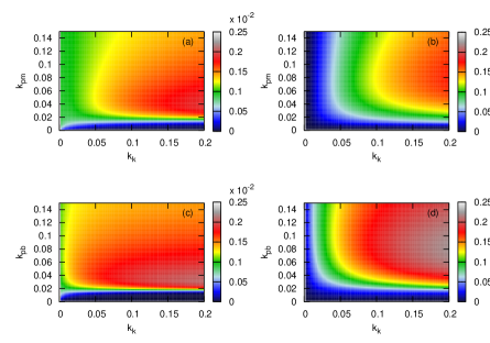
Figure 5: (color online) Two dimensional map of Fano factor and mutual information, repectively, for monofunctional (a,b) and bifunctional system (c,d) as a function of kinase and phosphatase rate. The two dimensional map is a projection of Fano factor and mutual information on the kinase and phosphatase plane. All panels are drawn using $\langle I\rangle$ = 1 $\mu$M. Values of other parameters are same as in Fig. 2.

To check the specific role of kinase and phosphatase rate on information processing within TCS further, we calculate Fano factor and ${\cal I}(I,R_{p})$ as a function of kinase and phosphatase rate. In Figs. 5(a)-5(b), we show two dimensional map of Fano factor and mutual information, respectively, for monofunctional system as a function of $k_{k}$ and $k_{pm}$. Figs. 5(c)-5(d) show the same for bifunctional system as a function of $k_{k}$ and $k_{pb}$. Fig. 5(a) shows that for high kinase and moderate phosphatase rate, the fluctuations level of phosphorylated response regulator becomes maximum otherwise it maintains a low value. This happens due to low copy number of proteins produced under high phosphatase regime. For the bifunctional system, the fluctuations level maintains a low value for a wide range of kinase and low phosphatase rate (see Fig. 5(c)). Other than that, the fluctuations increase due to increase in the phosphatase activity of the sensor protein. It is important to mention that maximum fluctuations level for the bifunctional system spans a wider region in the kinase-phosphatase plane compared to the monofunctional system. Figs. 5(b,d) show mutual information for monofunctional and bifunctional system, respectively. In both cases, signal processing capacity increases for high kinase and high phosphatase rate. In the regime of high kinase and high phosphatase activity, fluctuations in the $R_{p}$ copy number can reliably sense the fluctuations due to extra-cellular stimulus which, in turn, effectively increases the signal processing capacity. In addition, due to structural advantage, information processing is better for the bifunctional system.

Figure 6: Role of $P_{h}$ in (a) $\langle R_{p}\rangle$, (b) $\sigma_{R_{p}}^{2}$, (c) Fano factor and (d) ${\cal I}(I,R_{p})$ for monofunctional system. Open circle, up triangle and down triangle stand for $P_{h}=3.0$, 0.3 and 0.03, respectively (all in $\mu$M). Profile of bifunctional system (solid line with squares) has been shown in all four panels, for reference. Values of the other parameters are same as in Fig. (2).

Our analysis suggests that the bifunctional system can transduce external stimulus more reliably than the monofunctional one. Effective signal transduction mechanism of the bifunctional system can be attributed to its sensor domain which has synchronized kinase and phosphatase activity. On the other hand, the monofunctional system lacks such a synchronization due to the absence of phosphatase activity in the sensor domain. At this point, one can ask the question, ‘Is it possible to increase the activity of a monofunctional system by varying the contribution of one or more system components?’ To answer this question we further looked into the signal transduction motif of the monofunctional system and found that due to the auxiliary protein $P_{h}$, the monofunctional TCS is unable to attain the activity of the bifunctional one. Using this phenomenological information, one may hypothesize that by reducing the effect of $P_{h}$, activity of the monofunctional system can be increased. To check this hypothesis, we have systematically reduced the concentration of $P_{h}$ by reducing the synthesis rate ($k_{sP_{h}}$) of $P_{h}$ from high to low value and calculated all physical quantities reported in Fig. 2 (see Fig. 6). As the level of $P_{h}$ goes down, the phosphatase activity on the response regulator becomes more ineffective, and hence increases the pool of $R_{p}$ (see Fig. 6(a)). For a low amount of $P_{h}$, $R_{p}$ level reaches the maximum value, as attained by the bifunctional system, quite early. This suggests that using the parameter set of the model and by lowering the amount of $P_{h}$, a monofunctional system can attain a large pool of $R_{p}$ even at a very low level of inducer. At a very low level of $P_{h}$, most of the response regulators get phosphorylated, henceforth reducing fluctuations in the $R_{p}$ level (see Figs. 6(b),6(c)). Interestingly, mutual information for the monofunctional system goes down with lowering of $P_{h}$ (see Fig. 6(d)). By reducing the level of $P_{h}$, fluctuations in $R_{p}$ level can be reduced, which, in turn, makes the system independent of fluctuations due to external stimulus. As a result, one observes suppression of mutual information.

Fluctuations due to inherent noisy biochemical reactions play an important role in gene regulation by imposing phenotypic heterogeneity within genetically identical cells Kaern et al. (2005); Tiwari et al. (2010). This happens due to fluctuations induced distribution of proteins in identical cells. In the present study, the TCS network output ($R_{p}$) shows maximal and minimal level of fluctuations for low and high stimulus, respectively. In addition to that, the bifunctional system maintains a lower noise profile compared to the monofunctional one. These results together suggest that the bifunctional system controlled gene regulation may have lesser variability (lower Fano factor) compared to the monofunctional system for intermediate to high stimulus level. To verify difference in variability in TCS controlled gene regulation, we consider a simple model of gene expression in the following section.

III.1 TCS mediated gene regulation

To understand the role of TCS on downstream genes, we consider a simple model of gene regulation mediated by either monofunctional or bifunctional TCS

$$\overset{k_{1}f(R_{p})}{\longrightarrow}X\overset{k_{2}}{\longrightarrow}\varnothing,$$ (79)

where $X$ is the gene product whose synthesis is controlled by the transcription factor $R_{p}$, output of TCS. The function $f(R_{p})$ takes care of promoter switching mechanism associated with the downstream gene and is given by $f(R_{p})=R_{p}/(K+R_{p})$, with $K$ being the binding constant. While modeling promoter switching mechanism, we have considered positive regulation by $R_{p}$. The stochastic differential equation associated with Eq. (79) is given by

$$\frac{dX}{dt}=k_{1}f(R_{p})-k_{2}X+\xi_{X},$$ (80)

with $\langle\xi_{X}(t)\rangle=0$ and $\langle\xi_{X}(t)\xi_{X}(t^{\prime})\rangle=2k_{2}\langle X\rangle\delta(t-t^{\prime})$. Fourier transformation of the linearized version of Eq. (80) yields

$$\delta\tilde{X}(\omega)=k_{1}\left[\frac{\delta f(R_{p})}{\delta R_{p}}\right]_{ss}\frac{\delta\tilde{R}_{p}(\omega)}{(i\omega+k_{2})}+\frac{\tilde{\xi}_{X}(\omega)}{(i\omega+k_{2})},$$ (81)

where $\left[\delta f(R_{p})/\delta R_{p}\right]_{ss}=K/(K+\langle R_{p}\rangle)^{2}$, evaluated at steady state ($ss$). Now, using expression of $\delta\tilde{X}$, we derive variance associated with $X$,

$$\sigma^{2}_{X}=k_{1}^{2}\left[\frac{\delta f(R_{p})}{\delta R_{p}}\right]_{ss}^{2}\frac{\sigma_{R_{p}}^{2}}{k_{2}}+\langle X\rangle.$$ (82)

Note that in Eq. (82), fluctuations due to the output of TCS is embedded in the expression of $\sigma_{R_{p}}^{2}$, which is different for the monofunctional and the bifunctional system (see Eq. (44) and Eq. (76), respectively).

Figure 7: Steady state $\langle X\rangle$ as a function of inducer $\langle I\rangle$. The solid (with open circle) and dashed (with open square) lines are $\langle X\rangle$ profile generated by monofunctional and bifunctional system, respectively. Note that the lines and symbols are due to theory and simulation Gillespie (1976, 1977), respectively. The horizontal dotted line is for target $\langle X\rangle$ value and the vertical dotted lines are corresponding inducer level for monofunctional and bifunctional systems. (1), (2) and (3) corresponds to three different regions of $\langle I\rangle$ for a fixed target $\langle X\rangle$. Inset (b): Fano factor (Ff) for $X$ as a function of $\langle I\rangle$. Both lines and symbols are same as in main figure. Inset (1)-(3): Probability distribution of $R_{p}$ as a function of $\langle R_{p}\rangle$. The solid and dotted lines represent probability distribution of $R_{p}$ for monofunctional and bifunctional system, respectively. The vertical dotted line denotes value of target $\langle X\rangle$ as shown in the main figure. Parameters used are $K=5$ $\mu$M, $k_{1}=3\times 10^{-3}$ $\mu$M$s^{-1}$, $k_{2}=3\times 10^{-4}$ $s^{-1}$ and values of the other parameters are same as in Fig. 2.

Main panel of Fig. 7 shows steady state $\langle X\rangle$ as a function of mean inducer level $\langle I\rangle$ controlled by monofunctional (solid line with open circle) and bifunctional system (dashed line with open square). It is evident from the profiles of $\langle X\rangle$ that the bifunctional regulated system produces more downstream protein as $\langle I\rangle$ is increased. This happens due to availability of larger amount of $\langle R_{p}\rangle$ produced by the bifunctional system compared to the monofunctional one, for a fixed amount of $\langle I\rangle$ (see Fig. 2(a)). Fig. 7(b) depicts Fano factor ($\sigma^{2}_{X}/\langle X\rangle$) associated with downstream protein and shows that fluctuations in $X$ controlled by the bifunctional system is lower compared to the monofunctional system. Fluctuations in $X$ is controlled by fluctuations in $R_{p}$, as shown in Eq. (82). As fluctuations associated with $R_{p}$ due to the bifunctional system is lower than the monofunctional system (see Fig. 2(c)), its contribution in Fano factor associated with X is low.

In the previous discussion, we have shown that for a fixed level of inducer, a bifunctional system produces more $R_{p}$ compared to a monofunctional system (see Fig. 2(a)). From this observation, we commented that a bifunctional system is more effective than a monofunctional one in regulating downstream genes for intermediate to high inducer level. To verify our remark, we numerically calculate probability distribution of $R_{p}$ (transcription factor for target gene) for monofunctional and bifunctional system (solid and dashed lines in inset (1)-(3) of Fig. 7) for different values of $\langle I\rangle$ and check whether they are able to cross the fixed $\langle X\rangle$ value (vertical dotted line in inset (1)-(3) of Fig. 7). The distribution profiles give an idea of whether the pool of $R_{p}$ is able to generate a fixed level of gene product, in presence of inducer. For this, we set the value of downstream product $X$ at 3 $\mu$M (horizontal dotted line in the main panel of Fig. 7) which intercepts both profiles of $\langle X\rangle$ at two different values of $\langle I\rangle$. To be explicit, for $\langle I\rangle=3.2\mu$M and $5.6\mu$M, the horizontal dotted line intercepts the profile of bifunctional and monofunctional system, respectively. This, in turn, generates three different regions of $\langle I\rangle$, (1), (2) and (3) shown in the main panel of Fig. 7. When value of $\langle I\rangle$ lies within region (1), the distribution profiles of $R_{p}$ for both systems are unable to cross the required value of $\langle X\rangle$ (inset (1) of Fig. 7). This scenario changes as we move to region (2). In this region, the distribution profile of the bifunctional system crosses target $\langle X\rangle$ value, but the distribution profile of the monofunctional system is unable to cross the same (inset (2) of Fig. 7)). This happens due to low and high pool of $R_{p}$ generated by monofunctional and bifunctional system, respectively. As we further move to region (3), we see that the distribution profiles of both the systems are able to cross the target $\langle X\rangle$ value as both produce enough $R_{p}$ to achieve the goal.

IV Conclusion

To conclude, we have developed a stochastic model for signal transduction mechanism in bacterial TCS. The proposed model takes into account the difference in the functionality of the sensor kinase. This difference in functionality leads to a classification of the TCS, viz., monofunctional and bifunctional. Considering only the phosphotransfer mechanism within TCS triggered by external stimulus, we have derived Langevin equation associated with system components for both systems (monofunctional and bifunctional). Using the expression of phosphorylated response regulators, we have calculated different physically realizable quantities, viz., variance, Fano factor (variance/mean), mutual information at steady state. Our analysis suggests that at low external stimulus, both systems reliably transduce information due to changes made in the extra-cellular environment. Moreover, due to functional difference of the sensor kinase, it has been observed that fidelity of the bifunctional system is higher than that of the monofunctional system. Functionality of monofunctional system has been predicted to be increasable by reducing the amount of auxiliary protein ($P_{h}$) which can be tested experimentally. We further extend our analysis by studying TCS mediated gene regulation which shows that the bifunctional system is more effective in producing target gene product for intermediate to high inducer level with lesser variability.