Entanglement-assisted weak value amplification

Abstract

Large weak values have been used to amplify the sensitivity of a linear response signal for detecting changes in a small parameter, which has also enabled a simple method for precise parameter estimation. However, producing a large weak value requires a low postselection probability for an ancilla degree of freedom, which limits the utility of the technique. We propose an improvement to this method that uses entanglement to increase the efficiency. We show that by entangling and postselecting $n$ ancillas, the postselection probability can be increased by a factor of $n$ while keeping the weak value fixed (compared to $n$ uncorrelated attempts with one ancilla), which is the optimal scaling with $n$ that is expected from quantum metrology. Furthermore, we show the surprising result that the quantum Fisher information about the detected parameter can be almost entirely preserved in the postselected state, which allows the sensitive estimation to approximately saturate the optimal quantum Cramér-Rao bound. To illustrate this protocol we provide simple quantum circuits that can be implemented using current experimental realizations of three entangled qubits.

Weak value amplification is an enhanced detection scheme that was first suggested by Aharonov, Albert, and Vaidman AAV . (See Kofman2012 and justin for recent reviews.) The scheme exploits the fact that postselecting the weak measurement of an ancilla can produce a linear detector response with an anomalously high sensitivity to small changes in an interaction parameter. The sensitivity arises from coherent “super-oscillatory” interference in the ancilla Berry2012 , which is controlled by the choice of preparation and postselection of the ancilla. The price that one pays for this increase in sensitivity is a reduction in the potential signal (and thus the potential precision of any estimation) due to the postselection process Zhu2011 ; Tanaka2013 ; Ferrie2013 ; Knee2013 ; Combes2013 . Nevertheless, by using this technique one can still consistently recover a large fraction of the maximum obtainable signal in a relatively simple way Starling2009 ; Feizpour2011 . The relevant information is effectively concentrated into the small set of rarely postselected events Jordan2013 .

A growing number of experiments have successfully used weak value amplification to precisely estimate a diverse set of small physical parameters, including beam deflection (to picoradian resolution) science spin hall ; signaltonoise2 ; Turner2011 ; Pfeifer2011 ; Hogan2011 ; Zhou2012 ; Zhou2013 ; Jayaswal2014 , frequency shifts precision , phase shifts Starling2010 ; Xu2013 , angular shifts Magana2013 , temporal shifts Strubi2013 ; Viza2013 , and temperature shifts Egan2012 . More experimental schemes have also been proposed proposal-chargesensing ; proposal-electron spin ; proposal-phaseshift ; proposal-Tomography of Many-Body Weak Value ; proposal-wu-marek ; proposal-fermion ; Susa2012 ; Hayat2014 . These experimental results have shown remarkable resiliance to the addition of temporally-correlated noise, such as beam jitter Jordan2013 . Moreover, some of these experiments have reported precision near the standard quantum limit, which is surprising due to the intrinsic postselection loss. These observations have prompted the question of whether the amplification technique can be improved further by combining it with other metrology techniques. One such improvement that has been proposed is to recycle the events that were discarded by the postselection back into the measurement Dressel2013 . Another investigation has shown the that in certain cases it may even be possible to achieve precision near the optimal Heisenberg limit using seemingly classical resources Zhang2013 .

In this Letter we supplement these efforts by asking whether adding quantum resources to the weak value amplification procedure can also improve the efficiency of the technique. We find that using entangled ancilla preparations and postselections does indeed provide such an improvement. That is, the postselection probability can be increased while preserving the amplification factor, which effectively decreases the number of discarded events required to achieve the same sensitivity. Alternatively, one can enhance the amplification directly while preserving the same postselection probability. We show that these improvements scale optimally as the number of entangled ancillas increases; however, using even a small number of entangled ancillas provides a notable improvement. Moreover, we show that nearly all the quantum Fisher information about the estimated parameter can be preserved in the rarely postselected state, which allows the parameter estimation to nearly saturate the quantum Cramér-Rao bound in the weak value regime.

As a concrete proposal that demonstrates this optimal scaling, we consider using $n$ entangled ancilla qubits brun to estimate a small controlled phase applied to a meter qubit. Recent experiments with optical experiment-weak value , solid-state Groen2013 ; Campagne2013 and NMR Lu2013 systems have already verified the weak value effect using one or two qubits. As such, we provide a simple set of similar quantum circuits that can be implemented experimentally in a straightforward way using only three physical qubits.

Weak value amplification.— As a brief review, recall that for a typical weak value amplification experiment one uses an interaction Hamiltonian of the form

$$\hat{H}_{\mathrm{int}}=\hbar g\hat{A}\otimes\hat{F}\,\delta(t-t_{0}),$$ (1)

where $\hat{A}$ is an ancilla observable, $\hat{F}$ is a meter observable, and $g$ is the small coupling parameter that one would like to estimate. The time factor $\delta(t-t_{0})$ indicates that the interaction between the ancilla and the meter is impulsive, i.e., happening on a much faster timescale than the natural evolution of both the ancilla and the meter. Importantly for our discussion, we leave the dimension of $\hat{A}$ arbitrary.

An experimenter prepares the meter in a pure state $|\phi\rangle$ and the ancilla in a pure initial state $|\Psi_{i}\rangle$, then weakly couples them using the interaction Hamiltonian of Eq. (1), and then postselects the ancilla into a pure final state $|\Psi_{f}\rangle$, discarding the events where the postselection fails. This procedure effectively prepares an enhanced meter state that includes the effect of the ancilla $|\phi^{\prime}\rangle=\hat{M}|\phi\rangle/||\hat{M}|\phi\rangle||$, which we write here in terms of a Kraus operator $\hat{M}=\langle\Psi_{f}|\exp(-\mathrm{i}g\hat{A}\otimes\hat{F})|\Psi_{i}\rangle$. Averaging a meter observable $\hat{R}$ using this updated meter state yields $\langle\hat{R}\rangle_{|\phi^{\prime}\rangle}=\langle\phi|\hat{M}^{\dagger}\hat{R}\hat{M}|\phi\rangle/\langle\phi|\hat{M}^{\dagger}\hat{M}|\phi\rangle$.

For small $g$, this observable average is well approximated by the following second-order expansion DiLorenzo2012 ; Kofman2012

$$\langle\hat{R}\rangle_{|\phi^{\prime}\rangle}\approx\frac{2g\,\text{Im}(\alpha\,A_{w})+g^{2}\beta|A_{w}|^{2}}{1+g^{2}\sigma^{2}|A_{w}|^{2}},$$ (2)

where $\alpha=\langle\hat{R}\hat{F}\rangle_{|\phi\rangle}$, $\beta=\langle\hat{F}\hat{R}\hat{F}\rangle_{|\phi\rangle}$, and $\sigma^{2}=\langle\hat{F}^{2}\rangle_{|\phi\rangle}$ are correlation parameters that are fixed by the choice of meter observables and initial state, while

$$A_{w}=\frac{\langle\Psi_{f}|\hat{A}|\Psi_{i}\rangle}{\langle\Psi_{f}|\Psi_{i}\rangle}$$ (3)

is a complex weak value controlled by the ancilla AAV . Note that we have assumed that the initial meter state is unbiased $\langle\hat{F}\rangle_{|\phi\rangle}=\langle\hat{R}\rangle_{|\phi\rangle}=0$ to obtain the best response.

Most amplification experiments operate in the linear response regime where the second-order terms in Eq. (2) can be neglected, which produces josza

$$\langle\hat{R}\rangle_{|\phi^{\prime}\rangle}\approx 2g\left[\text{Re}A_{w}\,\text{Im}\alpha+\text{Im}A_{w}\,\text{Re}\alpha\right].$$ (4)

This linear relation shows how a large ancilla weak value can amplify the sensitivity of the meter for detecting small changes in $g$.

For concreteness, we consider a reference case when the meter is a qubit. State-of-the-art quantum computing technologies can already realize single qubit unitary gates and two qubit CNOT and controlled rotation gates with high fidelity (e.g., experiment-weak value ; Groen2013 ; Campagne2013 ; Lu2013 ; Reed2012 ; Chow2012 ; Murch2013 ; Zhong2013 ), so this example can be readily tested in the laboratory. The meter qubit is prepared in the state $|\phi\rangle=|+\rangle=(|0\rangle+|1\rangle)/\sqrt{2}$. The Pauli $Z$-operator $\hat{\sigma}_{z}=\hat{F}=\hat{R}$ will serve as both meter observables. These choices fix the constants $\alpha=1$, $\beta=0$, and $\sigma^{2}=1$ in Eq. (2), yielding the meter response

$$\langle\hat{\sigma}_{z}\rangle_{|+^{\prime}\rangle}\approx\frac{2g\,\text{Im}A_{w}}{1+g^{2}\,|A_{w}|^{2}}.$$ (5)

The nonlinearity in the denominator regularizes the detector response, placing a strict upper bound of $g|A_{w}|<1$ on the magnitudes that are useful for amplification purposes. The meter has a linear response in a more restricted range of roughly $g|A_{w}|<1/10$. In practice, one typically assumes that $g|A_{w}|\ll 1$.

As detailed in Figure 1, we couple a single ancilla qubit to the meter using a controlled-$Z$ rotation by a small angle $2\varphi$, which sets $g=\varphi/2$ and $\hat{A}=\hat{\sigma}_{z}$. The ancilla is initialized in the state $|\Psi_{i}\rangle=|+\rangle$ and postselected in the nearly orthogonal state $|\Psi_{f}\rangle=R_{z}(2\epsilon)|-\rangle=(\mathrm{e}^{-\mathrm{i}\epsilon}|0\rangle-\mathrm{e}^{\mathrm{i}\epsilon}|1\rangle)/\sqrt{2}$ with a probability $P_{s}=\sin^{2}(\epsilon)\approx\epsilon^{2}$, which produces the weak value $A_{w}=\mathrm{i}\cot(\epsilon)\approx\mathrm{i}/\epsilon$. The offset angle $\epsilon$ of the postselection must satisfy $\varphi/2<\epsilon<\pi/4$ for amplification, and $5\varphi<\epsilon<\pi/4$ for linear response.

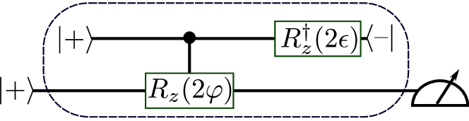
Figure 1: Quantum circuit that simulates the weak value amplification of a small parameter $\varphi$. A meter qubit is prepared in the state $|+\rangle=R_{y}(\pi/2)|0\rangle=(|0\rangle+|1\rangle)/\sqrt{2}$. An ancilla qubit is prepared in the same state $|\Psi_{i}\rangle=|+\rangle$. The ancilla is used as a control for a $Z$-rotation $R_{z}(2\varphi)$ of the meter, which simulates the unitary $\hat{U}=\exp(-\mathrm{i}\varphi\hat{A}\otimes\hat{\sigma}_{z}/2)$ with $\hat{A}=\hat{\sigma}_{z}$. The ancilla is then postselected in the nearly orthogonal state $\langle\Psi_{f}|=\langle-|R_{z}^{\dagger}(2\epsilon)=\langle 0|R_{y}^{\dagger}(-\pi/2)R_{z}^{\dagger}(2\epsilon)=(\langle 0|\mathrm{e}^{\mathrm{i}\epsilon}-\langle 1|\mathrm{e}^{-\mathrm{i}\epsilon})/\sqrt{2}$ with probability $P_{s}\approx\epsilon^{2}$ by performing two rotations, measuring in the $Z$-basis, and keeping only the $\langle 0|$ events. Finally, the meter qubit is measured in the $Z$-basis, which yields the linear response $\langle\hat{\sigma}_{z}\rangle_{+^{\prime}}\approx\varphi\,\text{Im}A_{w}$ that is amplified by the weak value $A_{w}\approx\mathrm{i}/\epsilon$. The probability for a single success of this circuit after $n$ attempts, $P_{s}^{(n)}=1-(1-P_{s})^{n}\approx n\,\epsilon^{2}$, is approximately linear in $n$.

Postselection probability.— While the weak value has the marvelous ability to effectively amplify the small parameter $g$ in a simple way, it also has a shortcoming of low efficiency. That is, for a large weak value $A_{w}$, Eq. (3) indicates that $\langle\Psi_{f}|\Psi_{i}\rangle$ must be small. This implies that the ancilla postselection probability is also small, since it approximates

$$P_{s}\approx|\langle\Psi_{f}|\Psi_{i}\rangle|^{2}$$ (6)

for small $g$. Therefore, the larger $A_{w}$ is, the less likely it is that one can successfully postselect the ancilla and prepare the amplified meter state $|\phi^{\prime}\rangle$.

We now show that adding quantum resources to the ancilla can improve this efficiency while keeping the amplification factor of the weak value $A_{w}$ the same. Specifically, we consider coupling $n$ entangled ancillas to the meter simultaneously. To make a fair comparison with the uncorrelated case, the probability of successfully postselecting $n$ entangled ancillas once should show an improvement over the probability of successfully postselecting a single ancilla once after $n$ independent attempts. The latter probability has linear scaling in $n$ when $P_{s}$ is small

$$P_{s}^{(n)}=1-(1-P_{s})^{n}\approx nP_{s}.$$ (7)

We will see that entangled ancillas can achieve quadratic scaling with $n$, which improves the postselection efficiency by a factor of $n$.

To show this improvement, we couple the meter to $n$ identical single-ancilla observables $\hat{a}$ using the interaction in Eq. (1), which effectively couples the meter to a single joint ancilla observable

$$\hat{A}=\hat{A}_{1}+\cdots+\hat{A}_{n},$$ (8)

where $\hat{A}_{k}=\hat{1}\otimes\cdots\hat{a}\cdots\otimes\hat{1}$ is shorthand for the observable $\hat{a}$ of the $k$^th ancilla. Notably the minimum and maximum eigenvalues of this joint observable, $\Lambda_{\min(\max)}=n\lambda_{\min(\max)}$, are determined by the eigenvalues of $\hat{a}$. Similarly, the corresponding eigenstates are product states of the eigenstates of $\hat{a}$: $|\Lambda_{\min(\max)}\rangle=|\lambda_{\min(\max)}\rangle^{\otimes n}$. The $n$ ancillas will be collectively prepared in a joint state $|\Psi_{i}\rangle$ and then postselected in a joint state $|\Psi_{f}\rangle$ to produce a joint weak value amplification factor $A_{w}$, just as in Eq. (3). An example circuit that implements this procedure with qubits is illustrated in Figure 2.

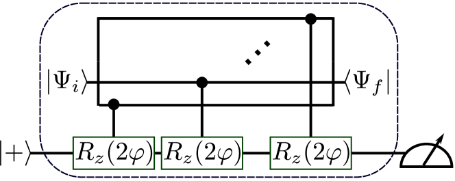
Figure 2: Quantum circuit that simulates the entanglement-assisted weak value amplification of a small parameter $\varphi$. As in Figure 1, a meter qubit is prepared in the state $|+\rangle$, while $n$ ancilla qubits are prepared in a entangled state $|\Psi_{i}\rangle$. Each ancilla is then used as a control for a $Z$-rotation $R_{z}(2\varphi)$ of the meter, simulating the unitary $\hat{U}=\exp(-\mathrm{i}\varphi\hat{A}\otimes\hat{\sigma}_{z}/2)$ with $\hat{A}$ being the sum of ancilla observables $\hat{\sigma}_{z}$. The ancillas are then postselected in an entangled state $|\Psi_{f}\rangle$, and the meter qubit is measured in the $Z$-basis, yielding the linear response $\langle\hat{\sigma}_{z}\rangle_{+^{\prime}}\approx\varphi\,\text{Im}A_{w}$ amplified by a joint weak value $A_{w}$.

The ability to improve the postselection efficiency hinges upon the fact that there can be different choices of $|\Psi_{i}\rangle$ and $|\Psi_{f}\rangle$ that will produce the same weak value $A_{w}$. However, these different choices will generally produce different postselection probabilities. Therefore, among these different choices of joint preparations and postselections there exists an optimal choice that maximizes the postselection probability.

We find this optimum in two steps. First, we maximize the postselection probability over all possible postselections $|\Psi_{f}\rangle$ while keeping the weak value $A_{w}$ and the preparation $|\Psi_{i}\rangle$ fixed. Second, we maximize this result over all preparations $|\Psi_{i}\rangle$.

To perform the first maximization, note that Eq. (3) implies $\langle\Psi_{f}|(\hat{A}-A_{w})|\Psi_{i}\rangle=0$, so $|\Psi_{f}\rangle$ must be orthogonal to $(\hat{A}-A_{w})|\Psi_{i}\rangle$. This gives a constraint on the possible postselections $|\Psi_{f}\rangle$, so the maximization of $P_{S}$ in Eq. (6) should be taken over the subspace $\mathcal{V}^{\perp}$ orthogonal to $(\hat{A}-A_{w})|\Psi_{i}\rangle$. As shown in the Supplementary Material supplement , the result of this maximization approximates

$$\max_{|\Psi_{f}\rangle\in\mathcal{V}^{\perp}}P_{s}\approx\frac{\text{Var}(\hat{A})_{|\Psi_{i}\rangle}}{|A_{w}|^{2}},$$ (9)

where $\text{Var}(\hat{A})_{|\Psi_{i}\rangle}=\langle\Psi_{i}|\hat{A}^{2}|\Psi_{i}\rangle-[\langle\Psi_{i}|\hat{A}|\Psi_{i}\rangle]^{2}$ is the variance of $\hat{A}$ in the initial state. This approximation applies when the weak value is larger than any eigenvalue of $\hat{A}$: $|\Lambda|\ll|A_{w}|<1/g$. However, since $\Lambda_{\min(\max)}=n\lambda_{\min(\max)}$, we must be careful to fix $|A_{w}|$ to be at least $n$ times larger than the eigenvalues of $\hat{a}$.

Now we consider maximizing the variance over an arbitrary initial state $|\Psi_{i}\rangle$, which produces quantum metrology 2

$$\max_{|\Psi_{i}\rangle}\text{Var}(\hat{A})_{|\Psi_{i}\rangle} =\frac{n^{2}}{4}(\lambda_{\max}-\lambda_{\min})^{2},$$ (10)

showing quadratic scaling with $n$. Therefore, according to Eq. (9) the maximum postselection probability also scales quadratically with $n$, showing a factor of $n$ improvement over the linear scaling of the uncorrelated ancilla attempts in Eq. (7).

The preparation states that show this quadratic scaling of the variance have the maximally entangled form quantum metrology 2

$$|\Psi_{i}\rangle =\frac{1}{\sqrt{2}}(|\lambda_{\max}\rangle^{\otimes n}+\mathrm{e}^{\mathrm{i}\theta}|\lambda_{\min}\rangle^{\otimes n}),$$ (11)

where $\mathrm{e}^{\mathrm{i}\theta}$ is an arbitrary relative phase. We provide a simple circuit to prepare such a state for $n$ qubits in Figure 3, choosing $\theta=0$.

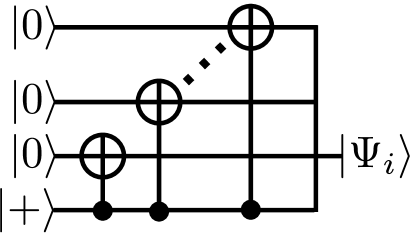
Figure 3: Quantum circuit to prepare the optimal entangled preparation for $n$ ancilla qubits. The state $|\Psi_{i}\rangle=(|0\rangle^{\otimes n}+|1\rangle^{\otimes n})/\sqrt{2}$ is prepared from a single $|+\rangle$ state by a sequence of CNOT gates. Due to this construction, we note that the ordering of the two-qubit gates in Figs. 2, 3, and 4 can be further optimized to pre- and postselect $(n-1)$ of the ancilla qubits sequentially, which allows the $n$-qubit entangled ancilla to be practically simulated using only three physical qubits.

According to the derivation in the Supplementary Material supplement , the corresponding postselection states that maximize the postselection probability are

$$|\Psi_{f}\rangle \propto-(n\lambda_{\min}-A_{w}^{*})|\lambda_{\max}\rangle^{\otimes n}$$ (12)

$$\qquad+\mathrm{e}^{\mathrm{i}\theta}(n\lambda_{\max}-A_{w}^{*})|\lambda_{\min}\rangle^{\otimes n},$$

which explicitly depend on the chosen value of $A_{w}$. We also provide a simple circuit to implement this postselection with $n$ qubits in Figure 4(a).

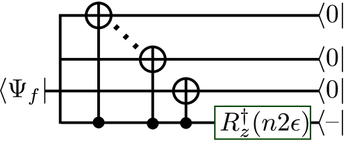
(a) Postselection maximizing $P_{s}$

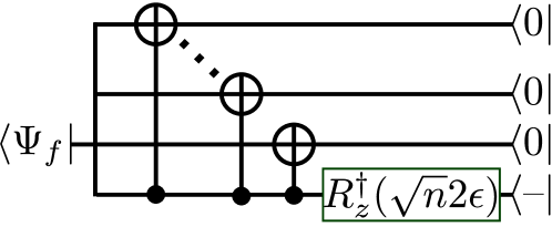
(b) Postselection maximizing $A_{w}$

Figure 4: Quantum circuits for attaining optimal postselections, using the preparation in Figure 3. (a) Keeping $A_{w}\approx\mathrm{i}/\epsilon$ fixed and maximizing $P_{s}$ produces the entangled postselection $\langle\Psi_{f}|=\langle 0|^{\otimes n}\mathrm{e}^{\mathrm{i}n\epsilon}-\langle 1|^{\otimes n}\mathrm{e}^{-\mathrm{i}n\epsilon}$ with $P_{s}\approx n^{2}\epsilon^{2}$, which is a factor of $n$ larger than the single ancilla $P_{s}^{(n)}$ in Figure 1. This postselection can be implemented as a sequence of CNOT gates and a rotation of the last qubit by $R_{z}^{\dagger}(n2\epsilon)$ and $R_{y}^{\dagger}(-\pi/2)$ before measuring all qubits in the $Z$-basis and keeping only $\langle 0|$ events. For small $\epsilon$ this state is equivalent to Eq. (12). (b) Keeping $P_{s}=P_{s}^{(n)}\approx n\epsilon^{2}$ and maximizing $A_{w}$ produces a similar state $\langle\Psi_{f}|=\langle 0|^{\otimes n}\mathrm{e}^{\mathrm{i}\sqrt{n}\epsilon}-\langle 1|^{\otimes n}\mathrm{e}^{-\mathrm{i}\sqrt{n}\epsilon}$ with $A_{w}\approx\mathrm{i}\sqrt{n}/\epsilon$, which is a factor of $\sqrt{n}$ larger than $A_{w}$ in Figure 1.

Weak value scaling.— So far we have shown that we can increase the postselection probability by a factor of $n$ when the weak value is kept fixed. Alternatively, we can hold the postselection probability fixed to increase the maximum weak value by factor of $\sqrt{n}$.

Given a specific postselection probability $P_{s}$, the postselected state $|\Psi_{f}\rangle$ must have the form

$$|\Psi_{f}\rangle=\sqrt{P_{s}}|\Psi_{i}\rangle+\sqrt{1-P_{s}}\mathrm{e}^{\mathrm{i}\theta}|\Psi_{i}^{\perp}\rangle,$$ (13)

where $|\Psi_{i}^{\perp}\rangle$ is an arbitrary state orthogonal to $|\Psi_{i}\rangle$. This implies that we can write the weak value in Eq. (3) as

$$A_{w}=\langle\Psi_{i}|\hat{A}|\Psi_{i}\rangle+\sqrt{\frac{1-P_{s}}{P_{s}}}\mathrm{e}^{-\mathrm{i}\theta}\langle\Psi_{i}^{\perp}|\hat{A}|\Psi_{i}\rangle.$$ (14)

For large $A_{w}$ and small $P_{s}$, then we can approximately neglect the first term. Since $\mathrm{e}^{\mathrm{i}\theta}$ is arbitrary, we can also assume that $\langle\Psi_{i}^{\perp}|\hat{A}|\Psi_{i}\rangle$ is positive. The maximum $\langle\Psi_{i}^{\perp}|\hat{A}|\Psi_{i}\rangle$ can be achieved when $|\Psi_{i}^{\perp}\rangle$ is parallel to the component of $\hat{A}|\Psi_{i}\rangle$ in the complementary subspace orthogonal to $|\Psi_{i}\rangle$. This choice produces $\langle\Psi_{i}^{\perp}|\hat{A}|\Psi_{i}\rangle=\|\hat{A}|\Psi_{i}\rangle-|\Psi_{i}\rangle\langle\Psi_{i}|\hat{A}|\Psi_{i}\rangle\|=[\text{Var}(\hat{A})_{|\Psi_{i}\rangle}]^{1/2}$. Therefore, the largest weak value that can be obtained from the initial state $|\Psi_{i}\rangle$ with a small postselection probability $P_{s}$ will approximate

$$\max|A_{w}|\approx\sqrt{\frac{\text{Var}(\hat{A})_{|\Psi_{i}\rangle}}{P_{s}}}.$$ (15)

That is, the variance controls the scaling for the maxima of both $P_{s}$ and $A_{w}$. Comparing Eqs. (9) and (22), it follows that if $P_{s}$ can be improved by a factor of $n$, then it is also possible to improve $A_{w}$ by a factor of $\sqrt{n}$. Furthermore, maximizing the variance produces the same initial state as Eq. (11), so the only difference between maximizing $P_{s}$ and $A_{w}$ is the choice of postselection state. We provide a simple circuit to implement this alternative postselection with $n$ qubits in Figure 4(b).

Fisher information.— An improvement factor of $\sqrt{n}$ in the estimation precision is the best that we can expect from using entangled ancillas, according to well-known results from quantum metrology quantum metrology 2 ; quantum metrology 3 ; footnote . We are thus faced with the conundrum of how such a rare postselection can possibly show such optimal scaling with $n$. After all, most of the (potentially informative) data is being discarded by the postselection.

To understand this behavior, we compare the quantum Fisher information $I(g)$ about $g$ contained in the post-interaction state $|\Phi_{g}\rangle=\exp(-\mathrm{i}g\hat{A}\otimes\hat{F})|\Psi_{i}\rangle|\phi\rangle$ to the Fisher information $I^{\prime}(g)$ that remains in the postselected state $\sqrt{P_{s}}|\phi^{\prime}\rangle$. As detailed in the Supplementary Material supplement , in the linear response regime $g|A_{w}|\text{Var}(\hat{F})^{\frac{1}{2}}\ll 1$ with an initially unbiased meter $\langle\hat{F}\rangle_{|\phi\rangle}=0$, and assuming a fixed $P_{s}\ll 1$ with maximal $|A_{w}|$, we obtain

$$I^{\prime}(g)\approx\eta\,I(g)\,[1-|gA_{w}|^{2}\text{Var}(\hat{F})]\leq I(g),$$ (16)

where $\eta=\text{Var}(\hat{A})_{|\Psi_{i}\rangle}/\langle\hat{A}^{2}\rangle_{|\Psi_{i}\rangle}$ is an efficiency factor.

Remarkably, $\eta$ can reach $1$ when $\langle\hat{A}\rangle_{|\Psi_{i}\rangle}=0$, implying that nearly all the original Fisher information $I(g)$ can be concentrated into one rarely obtained $|\phi^{\prime}\rangle$, up to a small reduction by $|gA_{w}|^{2}\text{Var}(\hat{F})\ll 1$. The remaining information is distributed among the discarded meter states, and could be retrieved in principle Ferrie2013 ; Combes2013 . For the example with $\hat{F}=\hat{a}=\hat{\sigma}_{z}$, the initial state in Eq. (11) yields $\eta=1$, $\text{Var}(\hat{F})=1$, and a total Fisher information of $I(g)=4\langle\hat{A}^{2}\rangle_{|\Psi_{i}\rangle}=4n^{2}$ (see the Supplementary Material supplement ). The Cramér-Rao bound is thus $[I^{\prime}(g)]^{-\frac{1}{2}}=(1/2n)[1-|gA_{w}|^{2}]^{-\frac{1}{2}}$ for the precision of any unbiased estimation of $g=\varphi/2$ using $|\phi^{\prime}\rangle$, confirming the optimal scaling with $n$.

Conclusion.— In summary, we have considered using entanglement to enhance the weak value amplification of a small parameter. If the amplification factor is held fixed, then $n$ entangled ancillas can improve the postselection probability by a factor of $n$ compared to $n$ attempts with uncorrelated ancillas. This improvement in postselection efficiency addresses a practical shortcoming of weak value amplification, and achieves the optimal scaling with $n$ that can be expected from quantum metrology. Indeed, we have shown that weak value amplification can nearly saturate the quantum Cramér-Rao bound, despite the low efficiency of postselection. We have also provided simple quantum circuits for the protocol that are readily implementable by existing quantum computing architectures that possess three qubits.

Acknowledgments.— JD thanks Alexander Korotkov, Eyob Sete, and Andrew Jordan for helpful discussions. This research was partially supported by the ARO MURI grant W911NF-11-1-0268. SP and TB also acknowledge the support from NSF grant CCF-0829870, while JD acknowledges support from IARPA/ARO grant W91NF-10-1-0334.

Appendix A Derivation of the maximum post-selection probability

To maximize $P_{s}\approx|\langle\Psi_{f}|\Psi_{i}\rangle|^{2}$ while keeping $A_{w}$ and $|\Psi_{i}\rangle$ fixed, we note that the initial state can be decomposed into a piece parallel to $(\hat{A}-A_{w})|\Psi_{i}\rangle$ and an orthogonal piece in the complementary subspace $\mathcal{V}^{\perp}$:

$$|\Psi_{i}\rangle =\frac{(\hat{A}-A_{w})|\Psi_{i}\rangle\langle\Psi_{i}|(\hat{A}-A_{w}^{*})|\Psi_{i}\rangle}{\langle\Psi_{i}|(\hat{A}-A_{w}^{*})(\hat{A}-A_{w})|\Psi_{i}\rangle}+\left(|\Psi_{i}\rangle-\frac{(\hat{A}-A_{w})|\Psi_{i}\rangle\langle\Psi_{i}|(\hat{A}-A_{w}^{*})|\Psi_{i}\rangle}{\langle\Psi_{i}|(\hat{A}-A_{w}^{*})(\hat{A}-A_{w})|\Psi_{i}\rangle}\right).$$ (17)

Since $|\Psi_{f}\rangle$ must also be in $\mathcal{V}^{\perp}$ by the definition of the weak value, it follows that the maximum $P_{s}$ can be achieved for the post-selection state parallel to the component of $|\Psi_{i}\rangle$ in $\mathcal{V}^{\perp}$, i.e.,

$$|\Psi_{f}\rangle\propto|\Psi_{i}\rangle-\frac{(\hat{A}-A_{w})|\Psi_{i}\rangle\langle\Psi_{i}|(\hat{A}-A_{w}^{*})|\Psi_{i}\rangle}{\langle\Psi_{i}|(\hat{A}-A_{w}^{*})(\hat{A}-A_{w})|\Psi_{i}\rangle}.$$ (18)

After some calculation, it follows that

$$\max_{|\Psi_{f}\rangle\in\mathcal{V}^{\perp}}P_{s}=\frac{\text{Var}(\hat{A})_{|\Psi_{i}\rangle}}{\langle\Psi_{i}|\hat{A}^{2}|\Psi_{i}\rangle-2\langle\Psi_{i}|\hat{A}|\Psi_{i}\rangle\mathrm{Re}A_{w}+|A_{w}|^{2}},$$ (19)

where $\text{Var}(\hat{A})_{|\Psi_{i}\rangle}=\langle\Psi_{i}|\hat{A}^{2}|\Psi_{i}\rangle-[\langle\Psi_{i}|\hat{A}|\Psi_{i}\rangle]^{2}$ is the variance of $\hat{A}$ in the state $|\Psi_{i}\rangle$.

For the purposes of weak value amplification, we usually require $|A_{w}|$ to be larger than any eigenvalue of $\hat{A}$, $|A_{w}|\gg|\Lambda|$. Therefore, this maximum $P_{s}$ can be approximated as Eq. (9) in the main text.

Appendix B Derivation of the optimal post-selection state

As noted in the previous section, the optimal post-selection state should be parallel to the component of $|\Psi_{i}\rangle$ in $\mathcal{V}^{\perp}$. The post-selection probability is then controlled by the variance $\text{Var}(\hat{A})_{|\Psi_{i}\rangle}$. This variance is maximized for a maximally entangled initial state $|\Psi_{i}\rangle=\frac{1}{\sqrt{2}}(|\lambda_{\max}\rangle^{\otimes n}+\mathrm{e}^{\mathrm{i}\theta}|\lambda_{\min}\rangle^{\otimes n})$. Hence, we can directly compute the optimal post-selected state to be

$$|\Psi_{f}\rangle \propto|\Psi_{i}\rangle-\frac{(\hat{A}_{\mathrm{total}}-A_{w})|\Psi_{i}\rangle\langle\Psi_{i}|(\hat{A}_{\mathrm{total}}-A_{w}^{*})|\Psi_{i}\rangle}{\langle\Psi_{i}|(\hat{A}_{\mathrm{total}}-A_{w}^{*})(\hat{A}_{\mathrm{total}}-A_{w})|\Psi_{i}\rangle}$$ (20)

$$=\frac{1}{\sqrt{2}}(|\lambda_{\max}\rangle^{\otimes n}+\mathrm{e}^{\mathrm{i}\theta}|\lambda_{\min}\rangle^{\otimes n})-\frac{1}{\sqrt{2}}((n\lambda_{\max}-A_{w})|\lambda_{\max}\rangle^{\otimes n}$$

$$\qquad+\mathrm{e}^{\mathrm{i}\theta}(n\lambda_{\min}-A_{w})|\lambda_{\min}\rangle^{\otimes n})\frac{n\lambda_{\max}+n\lambda_{\min}-2A_{w}^{*}}{|n\lambda_{\max}-A_{w}|^{2}+|n\lambda_{\min}-A_{w}|^{2}}$$

$$\propto(|n\lambda_{\min}-A_{w}|^{2}-(n\lambda_{\max}-A_{w})(n\lambda_{\min}-A_{w}^{*}))|\lambda_{\max}\rangle^{\otimes n}$$

$$\qquad+\mathrm{e}^{\mathrm{i}\theta}(|n\lambda_{\max}-A_{w}|^{2}-(n\lambda_{\min}-A_{w})(n\lambda_{\max}-A_{w}^{*}))|\lambda_{\min}\rangle^{\otimes n})$$

$$\propto-(n\lambda_{\min}-A_{w}^{*})|\lambda_{\max}\rangle^{\otimes n}+\mathrm{e}^{\mathrm{i}\theta}(n\lambda_{\max}-A_{w}^{*})|\lambda_{\min}\rangle^{\otimes n}.$$

This is Eq. (12) in the main text.

Appendix C Quantum Fisher information

It is important to determine just how well the weak value amplification technique can estimate the small parameter $g$. There is some concern that the post-selection process will lead to a substantial reduction of the total obtainable information, since a large fraction of the potentially usable data is being thrown away (e.g., Ferrie2013 ). To assuage these concerns, we compare the maximum Fisher information about $g$ that can be obtained without post-selection to the Fisher information that remains in the post-selected states used for weak value amplification.

We first recall a few general results from the study of quantum Fisher information. If one wishes to estimate a parameter $g$, then the minimum standard deviation of any unbiased estimator for $g$ is given by the quantum Cramér-Rao bound: $I(g)^{-1/2}$. The function $I(g)$ is the quantum Fisher information metrology2

$$I(g)=4\frac{\mathrm{d}\langle\Phi_{g}|}{\mathrm{d}g}\frac{\mathrm{d}|\Phi_{g}\rangle}{\mathrm{d}g}-4\left|\frac{\mathrm{d}\langle\Phi_{g}|}{\mathrm{d}g}|\Phi_{g}\rangle\right|^{2},$$ (21)

which is determined by a quantum state $|\Phi_{g}\rangle$ that contains the information about $g$. If this state is prepared with some interaction Hamiltonian $|\Phi_{g}\rangle=\exp(-ig\hat{H})|\Phi\rangle$ then the Fisher information reduces to a simpler form quantum metrology 2

$$I(g)=4\text{Var}(\hat{H})_{|\Phi\rangle},$$ (22)

and is entirely determined by the variance of the Hamiltonian in the pre-interaction state $|\Phi\rangle$.

C.1 General Discussion

In the main text, the relevant Hamiltonian with a meter observable $\hat{F}$ is $\hat{H}=\hbar g\hat{A}\otimes\hat{F}\delta(t-t_{0})$, where $\hat{A}$ is a sum of $n$ ancilla observables $\hat{a}$ of dimension $d$. The joint state $|\Phi\rangle$ is also always prepared in a product state $|\Phi\rangle=|\Psi_{i}\rangle\otimes|\phi\rangle$ between the ancillas and the meter. If there is no post-selection then the quantum Fisher information is found to be

$$I(g)=4\left[\langle\hat{A}^{2}\rangle_{|\Psi_{i}\rangle}\langle\hat{F}^{2}\rangle_{|\phi\rangle}-\left(\langle\hat{A}\rangle_{|\Psi_{i}\rangle}\langle\hat{F}\rangle_{|\phi\rangle}\right)^{2}\right].$$ (23)

Now suppose we projectively measure the ancillas in order to make a post-selection. This measurement will produce $d^{n}$ independent outcomes corresponding to some orthonormal basis $\{|\Psi_{f}^{(k)}\rangle\}_{k=1}^{d^{n}}$. In the linear response regime with $g\ll 1$, each of these outcomes prepares a particular meter state

$$|\phi^{\prime}_{k}\rangle \propto\langle\Psi_{f}^{(k)}|\exp(-ig\hat{H})|\Psi_{i}\rangle|\phi\rangle\approx(\hat{1}-igA_{w}^{(k)}\hat{F})|\phi\rangle$$ (24)

with probability $P_{s}^{(k)}\approx|\langle\Psi_{f}^{(k)}|\Psi_{i}\rangle|^{2}$ that is governed by a different weak value

$$A_{w}^{(k)}=\frac{\langle\Psi_{f}^{(k)}|\hat{A}|\Psi_{i}\rangle}{\langle\Psi_{f}^{(k)}|\Psi_{i}\rangle}.$$ (25)

We can then compute the remaining Fisher information contained in each of the post-selected states $\sqrt{P_{s}^{(k)}}|\phi^{\prime}_{k}\rangle$ using (21), which produces

$$I^{(k)}(g) \approx 4\,P_{s}^{(k)}|A_{w}^{(k)}|^{2}\,\left[\text{Var}(\hat{F})_{|\phi\rangle}-\langle\hat{F}^{2}\rangle_{|\phi\rangle}\left(2g\text{Im}A_{w}^{(k)}\langle\hat{F}\rangle_{|\phi\rangle}+|gA_{w}^{(k)}|^{2}\langle\hat{F}^{2}\rangle_{|\phi\rangle}\right)\right].$$ (26)

Importantly, if we add the information from all $d^{n}$ post-selections we obtain

$$\sum_{k=1}^{d^{n}}I^{(k)}(g) \approx 4\,\langle\hat{A}^{2}\rangle_{|\Psi_{i}\rangle}\,\text{Var}(\hat{F})_{|\phi\rangle}-O(g).$$ (27)

With the condition $\langle\hat{F}\rangle_{|\phi\rangle}=0$, this saturates the maximum in (23) up to small corrections, which indicates that the ancilla measurement does not lose information by itself. One can always examine all $d^{n}$ ancilla outcomes to obtain the maximum information, as pointed out in Ferrie2013 .

Now let us focus on a particular post-selection $k=1$, using an unbiased meter that satisfies $\langle\hat{F}\rangle_{|\phi\rangle}=0$, as assumed in the main text. This produces the simplification

$$I^{(1)}(g) \approx 4\,P_{s}^{(1)}|A_{w}^{(1)}|^{2}\,\left[1-|gA_{w}^{(1)}|^{2}\text{Var}(\hat{F})\right].$$ (28)

Now recall Eq. (15) of the main text, where we showed that if we fix $P_{s}^{(1)}\ll 1$ and picked a post-selection state that maximizes $A_{w}^{(1)}$ then we found

$$\max|A_{w}^{(1)}|^{2}\approx\frac{1-P_{s}^{(1)}}{P_{s}^{(1)}}\text{Var}(\hat{A})_{|\Psi_{i}\rangle}\approx\frac{\text{Var}(\hat{A})_{|\Psi_{i}\rangle}}{P_{s}^{(1)}}.$$ (29)

For this strategically chosen post-selection with small $P_{s}^{(1)}$ and maximized $A_{w}^{(1)}$, it then follows that

$$I^{(1)}(g) \approx 4\,\text{Var}(\hat{A})_{|\Psi_{i}\rangle}\,\left[1-|gA_{w}^{(1)}|^{2}\text{Var}(\hat{F})\right]=I(g)\;\left[\frac{\text{Var}(\hat{A})_{|\Psi_{i}\rangle}}{\langle\hat{A}^{2}\rangle_{|\Psi_{i}\rangle}}\right]\,\left[1-|gA_{w}^{(1)}|^{2}\text{Var}(\hat{F})\right],$$ (30)

which is Eq. (16) in the main text. That is, nearly all the Fisher information can be concentrated into a single (but rarely post-selected) meter state (see also Jordan2013 ). The remaining information is distributed among the $(d^{n}-1)$ remaining states, and could be retrieved in principle. The special post-selected meter state suffers an overall reduction factor of $\eta=\text{Var}(\hat{A})/\langle\hat{A}^{2}\rangle$, as well as a small loss $|gA_{w}^{(1)}|^{2}\text{Var}(\hat{F})$. However, most weak value amplification experiments operate in the linear response regime $g|A_{w}^{(1)}|\text{Var}(\hat{F})^{\frac{1}{2}}\ll 1$ where this remaining loss is negligible. Moreover, the overall reduction factor $\eta$ can even be set to unity by choosing ancilla observables that satisfy $\langle\hat{A}\rangle_{|\Psi_{i}\rangle}=0$.

As carefully discussed in Ferrie2013 , one cannot actually reach the optimal bound of (23) when making a post-selection. However, (30) shows that one can get remarkably close by carefully choosing which post-selection to make. It is quite surprising that one can even approximately saturate (23) while discarding the $(d^{n}-1)$ much more probable outcomes. Rare post-selections can often be advantageous for independent reasons (e.g., to attenuate an optical beam down to a manageable post-selected beam power), so this property of weak value amplification makes it an attractive technique for estimating an extremely small parameter $g$ that permits the linear response conditions Jordan2013 .

C.2 Examples

To see how this works in more detail, let us examine the ancilla qubit post-selection examples used in the main text, where $g=\varphi/2$. For completeness, we will work through two examples. First, we consider a sub-optimal ancilla observable $\hat{a}=|1\rangle\langle 1|$. Second, we consider an optimal ancilla observable $\hat{a}=\hat{\sigma}_{z}$ to emphasize the practical difference.

C.2.1 Ancilla Projectors

A suboptimal choice of ancilla observable is the projector $\hat{a}=|1\rangle\langle 1|$ used in controlled qubit operations. From the optimal initial state given by Eq. (10) in the main text, we have $\langle\hat{A}^{2}\rangle=n^{2}/2$ and $\langle\hat{A}\rangle=n/2$. Therefore, the maximum quantum Fisher information from (23) that we can expect for estimating $\varphi$ is

$$I(\varphi)=\frac{n^{2}}{2},$$ (31)

where the factor $1/2$ in $g=\varphi/2$ has been taken into account, and the corresponding quantum Cramér-Rao bound is $\sqrt{2}/n$. This is the best (Heisenberg) scaling of the estimation precision that can be obtained by using $n$ entangled ancillas with the given initial states.

Now, let us consider what happens when we make the optimal preparation and post-selections for weak value amplification. We expect from (30) that the maximum information which can be attained through post-selection will be reduced by a factor of

$$\eta=\frac{\text{Var}(\hat{A})_{|\Psi_{i}\rangle}}{\langle\hat{A}^{2}\rangle_{|\Psi_{i}\rangle}}=\frac{1}{2}.$$ (32)

It is in this sense that the choice of $\hat{a}$ as a projector is suboptimal. We will see in the next section what happens with the optimal choice of $\hat{\sigma}_{z}$.

In the first case considered in the main text (i.e., increasing the post-selection probability with the weak value $A_{w}$ fixed), the optimal post-selected state is

$$|\Psi_{f}\rangle\propto(A_{w}^{*})|1\rangle^{\otimes n}+(n-A_{w}^{*})|0\rangle^{\otimes n}.$$ (33)

Computing the post-selected meter state then produces

$$|\phi^{\prime}\rangle_{1}=\frac{\left[n-A_{w}[1-\cos(n\varphi/2)]\hat{1}-iA_{w}\sin(n\varphi/2)\hat{\sigma}_{z}\right]|\phi\rangle}{\left(n^{2}+2[|A_{w}|^{2}-n\text{Re}A_{w}][1-\cos(n\varphi/2)]\right)^{1/2}}\approx\left(\hat{1}-iA_{w}\frac{\varphi}{2}\hat{\sigma}_{z}\right)|\phi\rangle,$$ (34)

where we have used $\langle\phi|\hat{\sigma}_{z}|\phi\rangle=0$, and then have made the small parameter approximation $n\varphi\ll 1$. This recovers the expected linear response result in (24). This state is post-selected with probability

$$p_{1}=\frac{1}{2}-\cos(n\varphi/2)\frac{|A_{w}|^{2}-n\text{Re}A_{w}}{n^{2}+2[|A_{w}|^{2}-n\text{Re}A_{w}]}\approx\frac{n^{2}}{2n^{2}+4[|A_{w}|^{2}-n\text{Re}A_{w}]}\approx\frac{n^{2}}{4}|A_{w}|^{-2},$$ (35)

where we have made the small parameter approximation $n\varphi\ll 1$, and then the large weak value assumption $n\ll|A_{w}|$.

Now computing the quantum Fisher information (21) with the post-selected meter state $\sqrt{p_{1}}\,|\phi^{\prime}\rangle_{1}$ yields the simple expression

$$I_{1}(\varphi)\approx\frac{n^{2}}{4}\left(1-\left|\frac{\varphi A_{w}}{2}\right|^{2}\right)\leq\frac{n^{2}}{4},$$ (36)

in agreement with (30). The maximum achieves the best possible scaling of $n^{2}$ as in (31). Moreover, for the most frequently used linear response regime with $|A_{w}|\varphi\ll 1$, we achieve the expected maximum information of $\eta I(\varphi)=n^{2}/4$.

For the second case (i.e., increasing the weak value $A_{w}$ with the post-selection probability fixed), we can obtain the results simply by rescaling $A_{w}\to\sqrt{n}A_{w}$ to produce $p_{2}\propto n$, as shown in the main text. This produces,

$$|\phi^{\prime}\rangle_{2}\approx\left(\hat{1}-i\sqrt{n}A_{w}\frac{\varphi}{2}\hat{\sigma}_{z}\right)|\phi\rangle,$$ (37)

and

$$p_{2}\approx\frac{n^{2}}{4}|\sqrt{n}A_{w}|^{-2}=\frac{n}{4}|A_{w}|^{-2},$$ (38)

and yields the Fisher information

$$I_{2}(\varphi)\approx\frac{n^{2}}{4}\left(1-n\left|\frac{\varphi A_{w}}{2}\right|^{2}\right)\leq\frac{n^{2}}{4}.$$ (39)

The increase of the amplification factor $|A_{w}|$ correspondingly decreases the remaining Fisher information, as expected from (36). However, since $n\varphi\ll 1$ and $\varphi|A_{w}|\ll 1$ in the linear response regime, this decrease is still small.

Alternatively, this second case can be computed explicitly as follows. For a fixed post-selection probability $p$, the post-selected state must be $|\Psi_{f}\rangle=\sqrt{p}|\Psi_{i}\rangle+\sqrt{1-p}|\Psi_{i}^{\perp}\rangle,$ where the optimal $|\Psi_{i}^{\perp}\rangle$ is parallel to the component of $\hat{A}|\Psi_{i}\rangle$ in the complementary subspace orthogonal to $|\Psi_{i}\rangle$. Computing this yields

$$|\Psi_{f}\rangle =\sqrt{p}|\Psi_{i}\rangle+\sqrt{1-p}\frac{\hat{A}|\Psi_{i}\rangle-|\Psi_{i}\rangle\langle\Psi_{i}|\hat{A}|\Psi_{i}\rangle}{\sqrt{\text{Var}(\hat{A})_{|\Psi_{i}\rangle}}}$$ (40)

$$=\left(\sqrt{\frac{p}{2}}-\sqrt{\frac{1-p}{2}}\right)|0\rangle^{\otimes n}+\left(\sqrt{\frac{p}{2}}+\sqrt{\frac{1-p}{2}}\right)|1\rangle^{\otimes n}.$$

Thus, computing the post-selected meter state yields

$$|\phi^{\prime}\rangle_{2}\propto\left(\left(\sqrt{\frac{p}{2}}-\sqrt{\frac{1-p}{2}}\right)\hat{1}+\left(\sqrt{\frac{p}{2}}+\sqrt{\frac{1-p}{2}}\right)\mathrm{e}^{-in\varphi\hat{\sigma}_{z}/2}\right)|\phi\rangle\approx\left(\hat{1}-i|A_{w}|\frac{\varphi}{2}\hat{\sigma}_{z}\right)|\phi\rangle,$$ (41)

where we have defined the effective weak value factor

$$|A_{w}|=\frac{n}{2}\left(1+\sqrt{\frac{1-p}{p}}\right)\approx\frac{n}{2}p^{-1/2},$$ (42)

and have used the linear response approximations $n\varphi\ll 1$ and $\varphi|A_{w}|\ll 1$, as well as the small probability assumption $p\ll 1$. Computing the quantum Fisher information from (21) with the state $\sqrt{p}\,|\phi^{\prime}\rangle_{2}$ then produces

$$I_{2}(\varphi)\approx p|A_{w}|^{2}\left(1-\left[\frac{\varphi|A_{w}|}{2}\right]^{2}\right)=\frac{n^{2}}{4}\left(1-\left[\frac{n\varphi}{4\sqrt{p}}\right]^{2}\right)\leq\frac{n^{2}}{4}$$ (43)

using the definition (42). This result precisely matches the form of (28). It is now clear that for quadratic scaling $p=n^{2}p_{0}$ we recover (36) with the effective reference weak value $|A_{w}|=1/(2\sqrt{p_{0}})$, while for linear scaling $p=np_{0}$ we recover (39).

C.2.2 Ancilla Z-operators

For contrast, an optimal choice of ancilla observable is $\hat{a}=\hat{\sigma}_{z}$, as used in the main text. From the optimal initial state given by Eq. (10) in the main text, we have $\langle\hat{A}^{2}\rangle=n^{2}$ and $\langle\hat{A}\rangle=0$. Therefore, the maximum quantum Fisher information from (23) that we can expect for estimating $\varphi$ is

$$I(\varphi)=n^{2},$$ (44)

which is a factor of 2 larger than (31). The corresponding quantum Cramér-Rao bound is $1/n$. From (30), we expect that the reduction factor is

$$\eta=\frac{\text{Var}(\hat{A})_{|\Psi_{i}\rangle}}{\langle\hat{A}^{2}\rangle_{|\Psi_{i}\rangle}}=1.$$ (45)

Thus, it is possible to saturate the optimal bound with this choice of $\hat{a}$.

In the first case considered in the main text (i.e., increasing the post-selection probability with the weak value $A_{w}$ fixed), the optimal post-selected state is

$$|\Psi_{f}\rangle\propto(n+A_{w}^{*})|1\rangle^{\otimes n}+(n-A_{w}^{*})|0\rangle^{\otimes n}.$$ (46)

Computing the post-selected meter state then produces

$$|\phi^{\prime}\rangle_{1}=\frac{\left[n\cos(n\varphi/2)\hat{1}-iA_{w}\sin(n\varphi/2)\hat{\sigma}_{z}\right]|\phi\rangle}{\left(n^{2}\cos^{2}(n\varphi/2)+|A_{w}|^{2}\sin^{2}(n\varphi/2)\right)^{1/2}}\approx\left(\hat{1}-iA_{w}\frac{\varphi}{2}\hat{\sigma}_{z}\right)|\phi\rangle,$$ (47)

where we have used $\langle\phi|\hat{\sigma}_{z}|\phi\rangle=0$, and then have made the small parameter approximation $n\varphi\ll 1$. This again recovers the expected linear response result in (24). This state is post-selected with probability

$$p_{1}=\frac{n^{2}\cos^{2}(n\varphi/2)+|A_{w}|^{2}\sin^{2}(n\varphi/2)}{n^{2}+[A_{w}|^{2}}\approx\frac{n^{2}}{n^{2}+|A_{w}|^{2}}\approx n^{2}|A_{w}|^{-2},$$ (48)

where we have made the small parameter approximation $n\varphi\ll 1$, and then the large weak value assumption $n\ll|A_{w}|$.

Now computing the quantum Fisher information (21) with the post-selected meter state $\sqrt{p_{1}}\,|\phi^{\prime}\rangle_{1}$ yields the simple expression

$$I_{1}(\varphi)\approx n^{2}\left(1-\left|\frac{\varphi A_{w}}{2}\right|^{2}\right)\leq n^{2},$$ (49)

in agreement with (30). The maximum saturates the upper bound of $n^{2}$ in (44), as expected.

For the second case (i.e., increasing the weak value $A_{w}$ with the post-selection probability fixed), we can again obtain the results simply by rescaling $A_{w}\to\sqrt{n}A_{w}$ to produce

$$|\phi^{\prime}\rangle_{2} \approx\left(\hat{1}-i\sqrt{n}A_{w}\frac{\varphi}{2}\hat{\sigma}_{z}\right)|\phi\rangle,$$ (50)

$$p_{2} \approx n^{2}|\sqrt{n}A_{w}|^{-2}=n|A_{w}|^{-2},$$ (51)

and the Fisher information

$$I_{2}(\varphi)\approx n^{2}\left(1-n\left|\frac{\varphi A_{w}}{2}\right|^{2}\right)\leq n^{2}.$$ (52)

Alternatively, computing the optimal post-selection state for a fixed post-selection probability $p$ yields the same state as (40). Hence, computing the post-selected meter state yields

$$|\phi^{\prime}\rangle_{2}\propto\left(\left(\sqrt{\frac{p}{2}}-\sqrt{\frac{1-p}{2}}\right)e^{in\varphi\hat{\sigma}_{z}/2}+\left(\sqrt{\frac{p}{2}}+\sqrt{\frac{1-p}{2}}\right)\mathrm{e}^{-in\varphi\hat{\sigma}_{z}/2}\right)|\phi\rangle\approx\left(\hat{1}-i|A_{w}|\frac{\varphi}{2}\hat{\sigma}_{z}\right)|\phi\rangle,$$ (53)

where we have defined the effective weak value factor

$$|A_{w}|=n\sqrt{\frac{1-p}{p}}\approx np^{-1/2},$$ (54)

in contrast to (42). Computing the quantum Fisher information from (21) with the state $\sqrt{p}\,|\phi^{\prime}\rangle_{2}$ then produces

$$I_{2}(\varphi)\approx p|A_{w}|^{2}\left(1-\left[\frac{\varphi|A_{w}|}{2}\right]^{2}\right)=n^{2}\left(1-\left[\frac{n\varphi}{\sqrt{p}}\right]^{2}\right)\leq n^{2},$$ (55)

using the definition (54). As before, this result precisely matches the form of (28). It is now clear that for quadratic scaling $p=n^{2}p_{0}$ we recover (49) with the effective reference weak value $|A_{w}|=1/\sqrt{p_{0}}$, while for linear scaling $p=np_{0}$ we recover (52). Therefore, in both post-selected qubit examples considered in the main text we can nearly saturate the expected maximum of $I(\varphi)=n^{2}$ when the linear response conditions $n\varphi\ll 1$, $\varphi|A_{w}|\ll 1$, and the large weak value condition $n\ll|A_{w}|$ are met, despite the loss of data incurred by the post-selection.

References

(1)Y. Aharonov, D. Z. Albert, and L. Vaidman, Phys. Rev.
Lett. 60, 1351 (1988).
(2)A. G. Kofman, S. Ashhab, and F. Nori, Phys. Rep.
520, 43 (2012).
(3)J. Dressel, M. Malik, F. M. Miatto, A. N. Jordan
and R. W. Boyd, arXiv:1305.7154 (2013).
(4)M. V. Berry and P. Shukla, J. Phys. A: Math. Theor.
45, 015301 (2012).
(5)X. Zhu, Y. Zhang, S. Pang, C. Qiao, Q. Liu, and
S. Wu, Phys. Rev. A 84, 052111 (2011).
(6)S. Tanaka and N. Yamamoto, Phys. Rev. A 88,
042116 (2013).
(7)C. Ferrie and J. Combes, arXiv:1307.4016 (2013).
(8)G. C. Knee and E. M. Gauger, arXiv:1306.6321 (2013).
(9)J. Combes, C. Ferrie, Z. Jiang, and C. M. Caves,
arXiv:1309.6620 (2013).
(10)D. J. Starling, P. B. Dixon, A. N. Jordan,
and J. C. Howell, Phys. Rev. A 80, 041803 (2009).
(11)A. Feizpour, X. Xing, and A. M. Steinberg,
Phys. Rev. Lett. 107, 133603 (2011).
(12)A. N. Jordan, J. Martínez-Rincón, and
J. C. Howell, arXiv:1309.5011 (2013).
(13)O. Hosten and P. Kwiat, Science 319,
787 (2008).
(14)P. B. Dixon, D. J. Starling, A. N. Jordan,
and J. C. Howell, Phys. Rev. Lett. 102, 173601 (2009).
(15)M. D. Turner, C. A. Hagedorn, S. Schlamminger,
and J. H. Gundlach, Opt. Lett. 36, 1479 (2011).
(16)M. Pfeifer and P. Fischer, Opt. Express 19,
16508 (2011).
(17)J. M. Hogan, J. Hammer, S.-W. Chiow, S. Dickerson,
D. M. S. Johnson, T. Kovachy, A. Sugarbaker, and M. A. Kasevich, Opt.
Lett. 36, 1698 (2011).
(18)X. Zhou, Z. Xiao, H. Luo, and S. Wen, Phys. Rev.
A 85, 043809 (2012).
(19)L. Zhou, Y. Turek, C. P. Sun, and F. Nori, Phys.
Rev. A 88, 053815 (2013).
(20) G.Jayaswal, G.Mistura, and M.Merano, arXiv:1401.0450 (2014).
(21)D. J. Starling, P. B. Dixon, A. N. Jordan, and
J. C. Howell, Phys. Rev. A 82, 063822 (2010).
(22)D. J. Starling, P. B. Dixon, N. S. Williams,
A. N. Jordan, and J. C. Howell, Phys. Rev. A 82, 011802(R)
(2010).
(23)X.-Y. Xu, Y. Kedem, K. Sun, L. Vaidman, C.-F. Li,
and G.-C. Guo, Phys. Rev. Lett. 111, 033604 (2013).
(24)O. S. Magana-Loaiza, M. Mirhosseini, B. Rodenburg, and R. W. Boyd, arXiv:1312.2981 (2013).
(25)G. Strübi and C. Bruder, Phys. Rev. Lett.
110, 083605 (2013).
(26)G. I. Viza, J. Martínez-Rincón, G. A.
Howland, H. Frostig, I. Shomroni, B. Dayan, and J. C. Howell, Opt.
Lett. 38, 2949 (2013).
(27)P. Egan and J. A. Stone, Opt. Lett. 37,
4991 (2012).
(28)A. Romito, Y. Gefen, and Y. M. Blanter, Phys. Rev.
Lett. 100, 056801 (2008).
(29)V. Shpitalnik,
Y. Gefen and A. Romito, Phys. Rev. Lett. 101, 226802 (2008).
(30)N. Brunner and C. Simon, Phys. Rev.
Lett. 105, 010405 (2010).
(31)O. Zilberberg, A. Romito, and Y.
Gefen, Phys. Rev. Lett. 106, 080405 (2011).
(32)S. Wu and M. Zukowski, Phys. Rev. Lett.
108, 080403 (2012).
(33)A. Hayat, A. Feizpour and A. M. Steinberg,
Phys. Rev. A 88, 062301 (2013)
(34)Y. Susa, Y. Shikano, and A. Hosoya, Phys. Rev.
A 85, 052110 (2012).
(35)A. Hayat, A. Feizpour, and A. M. Steinberg, arXiv:1311.7438 (2014).
(36)J. Dressel, K. Lyons, A. N. Jordan, T. M. Graham,
and P. G. Kwiat, Phys. Rev. A 88, 023821 (2013).
(37)L. Zhang, A. Datta, and I. M. Walmsley, arXiv:1310.5302
(2013).
(38) T. A. Brun, L. Diosi and W. T. Strunz, Phys. Rev.
A 77, 032101 (2008).
(39)G. J. Pryde, J. L. O’Brien, A. G.
White, T. C. Ralph, and H. M. Wiseman, Phys. Rev. Lett. 94,
220405 (2005).
(40)J. P. Groen, D. Ristè, L. Tornberg, J. Cramer,
P. C. de Groot, T. Picot, G. Johansson, and L. DiCarlo, Phys. Rev.
Lett. 111, 090506 (2013).
(41)P. Campagne-Ibarcq, L. Bretheau, E. Flurin,
A. Auffèves, F. Mallet, and B. Huard, arXiv:1311.5605 (2013).
(42)D. Lu, A. Brodutch, J. Li, H. Li, and R. Laflamme,
arXiv:1311.5890 (2013).
(43)A. Di Lorenzo, Phys. Rev. A 85, 032106
(2012).
(44)R. Jozsa, Phys. Rev. A 76, 044103 (2007).
(45)M. D. Reed, L. DiCarlo, S. E. Nigg, L. Sun, L.
Frunzio, S. M. Girvin, and R. J. Schoelkopf, Nature 482,
382 (2012).
(46)J. M. Chow, J. M. Gambetta, A. D. Corcoles, S.
T. Merkel, J. A. Smolin, C. Rigetti, S. Poletto, G. A. Keefe, M. B.
Rothwell, J. R. Rozen, M. B. Ketchen, and M. Steffen, Phys. Rev. Lett.
109, 060501 (2012).
(47)K. W. Murch, S. J. Weber, C. Macklin, and I. Siddiqi,
Nature 502, 2011 (2013).
(48)Y. P. Zhong, Z. L. Wang, J. M. Martinis, A. N.
Cleland, A. N. Korotkov, and H. Wang, arXiv:1309.0198 (2013).
(49)See the Supplementary Material for detailed derivations
of the optimal probabilities and postselection states, as well as
a more complete discussion of the quantum Fisher information and the
Cramér-Rao bound.
(50)V. Giovannetti, S. Lloyd, and L. Maccone,
Nature Photonics 5, 222 (2011).
(51)S. Boixo, S. T. Flammia, C. M. Caves,
and JM Geremia, Phys. Rev. Lett. 98, 090401 (2007).
(52)Note that some references have also considered
higher precision scalings such as that arise when there
are -body interactions between the ancillas quantum metrology 3 .
(53)S. L. Braunstein, C. M. Caves and G. J. Milburn,
Ann. Phys. 247, 135 (1996).