Anisotropic Rabi model

Abstract

We define the anisotropic Rabi model as the generalization of the spin-boson Rabi model: The Hamiltonian system breaks the parity symmetry; the rotating and counter-rotating interactions are governed by two different coupling constants; a further parameter introduces a phase factor in the counter-rotating terms. The exact energy spectrum and eigenstates of the generalized model is worked out. The solution is obtained as an elaboration of a recent proposed method for the isotropic limit of the model. In this way, we provide a long sought solution of a cascade of models with immediate relevance in different physical fields, including i) quantum optics: two-level atom in single mode cross electric and magnetic fields; ii) solid state physics: electrons in semiconductors with Rashba and Dresselhaus spin-orbit coupling; iii) mesoscopic physics: Josephson junctions flux-qubit quantum circuits.

I Introduction

There are very simple settings in physics whose understanding has very far reaching implications. This is the case of the Rabi type models, that are possibly the simplest ’organisms’ describing the interaction between a spin-half degree of freedom with a single boson. Originally formulated in quantum optics to describe the atom-field interaction Rabi , such kind of models play a crucial role in many other fields, especially with the advent of the quantum technologies. Here, we introduce an anisotropic generalization of the Rabi model and discuss the exact energies and eigenstates of it. In this way, we provide a long sought solution of a cascade of models with immediate relevance in various fields.

The Rabi type models provide the paradigm for key applications in a variety of different physical contexts, including quantum optics Scully , solid state and mesoscopic physics Wagner . Despite its importance, such models remained intractable with exact means for many years. Nevertheless, the physical community could thoroughly analyze the Rabi model physics, essentially because the physical settings allowed to easily adjust the field frequency to be resonating with the atomic band-width. In this way, assuming as well that the field intensity is weak, the Rabi model could be drastically simplified to the Jaynes-Cummings (JC) model JC , through the celebrated ’rotating wave’ approximation. The situation radically changed in the last decade, when Quantum Technology has been advancing towards more and more realistic applications Raimond ; Liebfried ; Englund . In most of the cases, if not all, the rotating wave approximation cannot be applied. In the solid state applications, for example, the electric field is an intrinsic quantity, that cannot be adjusted. On the other hand, in the applications in mesoscopic physics (like superconducting or QED circuits), the most interesting regimes correspond to very strong coupling between the spin variable and the bosonic degree of freedom.

The class of the anisotropic Rabi model we consider in the present paper are described by the following Hamiltonian

$$H=\omega a^{\dagger}a+\epsilon\sigma_{x}+\Delta\sigma_{z}+g(H_{r}+\lambda H_{cr}),$$

$$H_{r}=(a^{\dagger}\sigma^{-}+a\sigma^{+})\;,$$

$$H_{cr}=e^{i\theta}a^{\dagger}\sigma^{+}+e^{-i\theta}a\sigma^{-}\;$$ (1)

Here $a^{\dagger}$ and $a$ are the creation and annihilation operators for a bosonic mode of frequency $\omega$, $\sigma^{\pm}=(\sigma_{x}\pm i\sigma_{y})/2$, $\sigma_{x,y,z}$ are Pauli matrices for a two-level system, $2\Delta$ is the energy difference between the two levels, $g$ denotes the coupling strength of the rotating wave interaction $a^{\dagger}\sigma^{-}+a\sigma^{+}$ between the two-level system and the bosonic mode. For simplicity, we already take the unit of $\hbar=1$. In the Hamiltonian (1), the relative weight between rotating and counter-rotating terms, denoted respectively as $H_{c}$ and $H_{cr}$, can be adjusted by tuning the parameter $\lambda$. When $\epsilon=0$, the Hamiltonian enjoys a discrete $Z_{2}$ symmetry meaning that the parity of bosonic and spin excitations is conserved.

Several attempts of solving these type of models were tried employing Bethe ansatz and Quantum Inverse Scattering techniques Irish ; Amico-Frahm . The isotropic Rabi model corresponding to $\theta=0$ and $\lambda=1$ was solved exactly in a seminal paper by Braak Braak . Such an achievement has allowed to explore the physics of the Rabi model in full generality.

In this article, we present the exact solution of the anisotropic Rabi models (1). We discuss how the models can be applied to important physical settings in quantum optics, mesoscopic and solid state physics. We also observe that such model can be realized with cold atoms with arbitrary spin-orbit couplings.

II Exact analysis of the spectral problem

To focus on the main results, we first provide a schematic of the exact solution of the spectral problem

$$H|\Psi\rangle=E|\Psi\rangle\;,$$ (2)

while leaving the details in the appendix.

Our approach elaborates on the method originally developed by Braak Braak . In order to find a concise solution, we perform a unitary transformation on the spin degree of freedom in the Hamiltonian $(\ref{ha})$. The eigenvalues can be found as,

$$E_{n}=x_{n}-\frac{\lambda g^{2}}{\omega}.$$ (3)

where $x_{n}$ include regular and exceptional solutions. The regular solutions are solely zeros of the transcendental function, while the exceptional solutions are both the zeros and poles leading to a finite transcendental function and energy degeneracy. The transcendental function is as follows,

$$G_{\epsilon}(x)=\phi_{1}\overline{\phi}_{2}-\phi_{2}\overline{\phi}_{1}$$ (4)

where $\phi_{1}(z)=\exp(-\frac{\sqrt{\lambda}g\xi}{\omega}z)\sum_{n=0}^{\infty}L_{n}^{+}(z+\frac{\sqrt{\lambda}g\xi^{*}}{\omega})^{n}$, $\phi_{2}(z)=\exp(-\frac{\sqrt{\lambda}g\xi}{\omega}z)\sum_{n=0}^{\infty}K_{n}^{+}(z+\frac{\sqrt{\lambda}g\xi^{*}}{\omega})^{n}$, and $\phi_{1}(-z)=\overline{\phi}_{1}(z)$, $\phi_{2}(-z)=\overline{\phi}_{2}(z)$. Fig. 1 and Fig. 2 displays the actual behavior of $G_{\epsilon}(x)$ in different parameter regimes. For $\epsilon=0$, the $Z_{2}$ symmetry is recovered; in this case the transcendental function can be discussed through the functions $G_{+}=-e^{i\theta/2}\phi_{1}+\sqrt{\lambda}\phi_{2}$, $G_{-}=e^{-i\theta/2}\phi_{2}+\sqrt{\lambda}\phi_{1}$, living in the two parity sectors, separately (see Fig. 2). The explicit form of eigenfunctions $\phi_{1,2}(z)$ can also be obtained.

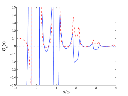
Figure 1: (Color online) Trascendental function $G_{\epsilon}(x)$ for $\epsilon\neq 0$. The parameters are $\omega=1$, $g=0.1$, $\lambda=0.5$, $\Delta=0.4$, $\epsilon=0.2$, and $\theta=-\pi/2$, the zero points whose real (blue-solid line) and imaginary part (red-dashed line) of $G_{\epsilon}$ both equal 0 correspond the eigenvalues of Hamiltonian.

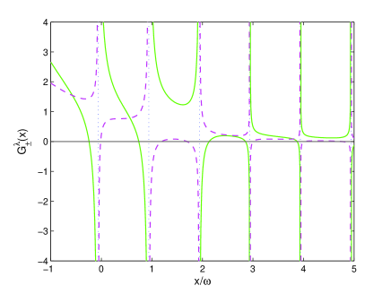
Figure 2: (color online) Trascendental functions $G_{+}^{\lambda}(x)$ (green-solid line) and real part of $G_{-}^{\lambda}(x)$ (purple-dashed line) for $\epsilon=0$. The parameters are $\omega=1$, $g=0.7$, $\Delta=0.4$, $\lambda=0.5$ and $\theta=-\pi/2$. The regular parts of the energy spectrum are determined by the zeros of the transcendental function $G_{\pm}^{\lambda}(x)$, the dotted vertical lines denote the poles $x\approx n-0.0612$, $n=0,1,2,...$, see (77). Notice that the imagine part of $G_{-}^{\lambda}(x)$ gives the same zero and poles as the real part, which is not shown.

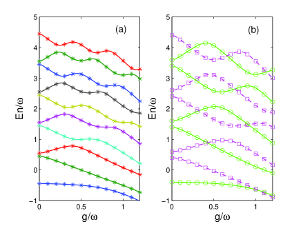
Figure 3: (Color online) Comparison between exact solution and the numerical results. (a) Energy spectrum for $\omega=1$, $\Delta=0.4$, $\lambda=0.5$, $\epsilon=0.2$ and $\theta=-\pi/2$. Solid lines are exact results, and the energy levels are differentiated by colors. Numerical results are represented by stars. (b) Energy spectrum for $\omega=1$, $\Delta=0.4$, $\lambda=0.5$, $\epsilon=0$, and $\theta=0$ in the spaces with positive (green lines with circles) and negative (purple lines with squares) parities. Small squares and circles represent numerical results The first energy level crossing point is at $g_{c}=4/\sqrt{15}\approx 1.0328$ and $E=-2/3$ which has no definite parity.

For vanishing $\epsilon$ or multiple of $\omega/2$, the system enjoys a $Z_{2}$ (parity) symmetry. In this case, the energy spectrum can be labeled by the two eigenvalues of the parity operator (corresponding to green-with-circle and purple-with-square lines in Fig. 3(b)). At the points of level crossings the energy is doubly degenerate. For the isotropic case, those solutions were found previously by Judd Judd ; Braak . For our anisotropic Rabi model, the crossing points are found as $E_{n}=n\omega-(1+\lambda^{2})^{2}/2\omega$, corresponding to exceptional spectrum. This exceptional spectrum is characterized by the merging of a pole with a zero resulting in a finite, nonzero transcendental function in Eq. (4) at energies corresponding to Juddian solutions Judd , see also Section VI.

For non vanishing generic values of $\epsilon$, the $Z_{2}$ symmetry is lost. This is manifested in the spectrum; in particular, there are no degeneracies (see Fig. 3(a)). As we shall see, the parameter $\theta$ is important to capture general spin-orbit couplings. We remark that with $Z_{2}$ symmetry preserved, $\theta$ can be deleted by a unitary transformation, and thus it does not change the energy spectrum. When $Z_{2}$ symmetry is broken with non-vanishing $\epsilon$, the parameter $\theta$ enters the energy spectrum through $\epsilon\sigma_{x}$ and this unitary transformation will induce term $\sigma_{x}\rightarrow\cos(\theta/2)\sigma_{x}+\sin(\theta/2)\sigma_{y}$.

As it will be later argued to be important for many applications, we quantify on the energy correction due to the counter-rotating term (Bloch-Siegert shift Bloch-Siegert ). Based on the exact solution, we can give closed expressions in several interesting limits. For $2\Delta\approx\omega$, $g\ll\omega$ the shift is $g^{2}/\omega$. For $\epsilon=0$, at the degenerate points, and setting $|\Delta|=(1-\lambda^{2})g^{2}/2\omega$, the ground state energy gap between the JC model and the anisotropic Rabi model can be found as,

$$\Delta E_{0}=\frac{\lambda^{2}g^{2}}{\omega}.$$ (5)

For $\lambda=1$, it is just the standard Bloch-Siegert shiftBloch-Siegert ; Shirley . Such gap can be obtained also for the excitations. For the first and the second excited states at degenerate points, it reads $\sim\lambda^{2}g^{4}/\omega^{3}$.

III Applications

In this section, we discuss how our solution can contribute to approach important problems in different physical contexts. Specifically, we will consider applications in quantum optics, mesoscopic physics, and spintronics.

III.1 Application to quantum optics: two level atom in cross electric and magnetic field.

When an atom is subjected of a crossed electric and magnetic field, the selection rules are not dictated by the possible values of the atomic angular momentum. Therefore, both the electric dipole and magnetic dipole transition are allowed. The Hamiltonian describing the system is

$$H=H_{0}-\mathbf{d}\cdot\mathbf{E}-\mathbf{\mu}\cdot\mathbf{B}$$ (6)

where we have assumed that the quadrupole transitions can be neglected. Inserting the standard expressions of the quantized electric and magnetic fields are respectively $E\sim(a+a^{\dagger})$ and $B\sim i(a-a^{\dagger})$ , Eq.(6) can be recast into our anisotropic Rabi model Eq.(1) with

$$g = {{\langle+|d|-\rangle+\langle+|\mu|-\rangle}\over{2}}$$ (7)

$$\lambda = {{\langle+|d|-\rangle-\langle+|\mu|-\rangle}\over{\langle+|d|-\rangle+\langle+|\mu|-\rangle}}$$ (8)

being $H_{0}|\pm\rangle=E_{\pm}|\pm\rangle$.

III.2 Application to superconducting circuits.

Superconducting circuits exploits the inherent coherence of superconductors for a variety of technological applications, including quantum computationesteve In this case, the bosonic fields typically represent the electromagnetic fields generated by the superconducting currents. The spin degree of freedom describes the two states of the qubit.

As immediate application, we consider two inductively coupled dc-Superconducting Quantum Interference Devices (SQUIDs)CHIORESCU ; MURALI : a primary SQUID $p$ (assumed large enough to produce an electromagnetic field characterized by a bosonic mode) controls the qubit realized by the secondary SQUID. In the limit of negligible capacitive coupling between the two SQUID’s, the circuit Hamiltonian is

$${\cal H}_{circuit}=\omega_{p}a^{\dagger}a-2E^{s}_{J}\sigma^{x}-2\tilde{L}_{p}(a+a^{\dagger})\sigma^{x}-iM(a-a^{\dagger})\sigma^{y}$$ (9)

where $\omega_{p}$ is the “frequency” of the primary and $E_{J}^{s}=E_{J}^{s}(\phi_{ext})$ provides the level splitting of the secondary SQUID, controlled by the external magnetic field; $\tilde{L}_{p}$ and $M$ are fixed by the inductance of the circuit and the mutual inductance respectively; the gate voltage $V_{g}$ is tuned to the charge degeneracy point. The Eq.(9) can be recast into the anisotropic Rabi modelAmicoHikami : $\displaystyle{\{\omega_{p},E^{s}_{J},2\tilde{L}_{p},M\}\rightarrow\{\omega,\epsilon,g(1+\lambda),g(1-\lambda)\}}$.

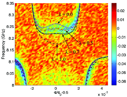
Figure 4: (Color online) Comparison between the anisotropic Rabi model with experimental results. The spectra (dashed dot lines) of the anisotropic Rabi model with $\lambda=0.0,0.5,0.7,1.0$, the other parameters are $g=0.74$GHz, $\Delta=4.21$GHz, $I_{p}=500$nA, $\omega_{r}=8.13$GHz, the same as previous investigated Mooij . The curves with $\lambda=0.5$ (red dashed dot line) agree perfectly with the experimental data (circle points).

We comment that the implications of the simultaneous presence of the rotating and counter-rotating terms have been evidenced experimentally Mooij ; Niemczyk ; Hakonen . The experimental system is an LC resonator magnetically coupled to a superconducting flux qubit in the ultrastrong coupling regime. Indeed the experimental data were interpreted as Bloch-Siegert energy correction of the Jaynes-Cummings dynamics. Here we point out that the experimental results can be fitted very well in terms of our anisotropic Rabi model, see Fig.4 (further details are provided in the appendix B.1). This provides an indication that, the inductance of the circuit is, indeed, very different from the mutual inductance between the primary and the qubit.

III.3 Applications to electrons in semiconductors with spin-orbit coupling.

Spin-orbit coupling effects have been opening up new perspectives in solid state physics, both for fundamental research (including topological insulators and spin-Hall effectstopo_ins ; spinHall ) and applications (notably spintronicsDatta ). Electronic spin orbit coupling can be induced by the electric field acting at the two dimensional interfaces of semiconducting heterostructure devicesDatta ; Rashba ; Dresselhaus ; Molenkamp ; Loss . The effective Hamiltonian reads

$$H = {{1}\over{2m}}\pi^{2}+{{1}\over{2}}g\mu_{B}B\sigma_{z}+H_{so}$$

$$H_{so} = H_{R}+H_{D}$$

$$H_{R} = \alpha(\pi_{x}\sigma_{y}-\pi_{y}\sigma_{x})\;,\;H_{D}=\beta(\pi_{x}\sigma_{x}-\pi_{y}\sigma_{y})$$ (10)

where $\mathbf{\pi}=\{\pi_{x},\pi_{y},\pi_{z}\}$ is the electrons canonical momentum $\mathbf{\pi}=\left(\mathbf{p}-{{q}\over{c}}\mathbf{A}\right)$. $H_{R}$ and $H_{D}$ are the Rashba Rashba and Dresselhaus Dresselhaus spin-orbit interactions. The coupling constant $\alpha$ depends on the electric field across the well, while the Dresselhaus coupling $\beta$ is determined by the geometry of the hetereostructure. The perpendicular magnetic field couples both to the electronic spin and orbital angular momentum. Applying the standard procedure leading to the Landau levels, the Hamiltonian (10) can be recast into our anisotropic Rabi model: $\alpha=\sqrt{g^{2}+(1+\lambda)^{2}}\sin{\theta}$, $\beta=\sqrt{g^{2}+(1+\lambda)^{2}}\cos{\theta}.$ Incidentally, we observe that the simultaneous presence of Dresselhaus and Rashba contributions couples all the Landau levels, making our exact solution immediately relevant for the physics of the system.

We comment that the Hamiltonian (10), has been realized with cold fermionic atoms systems, opening the avenue to study the spin-orbit effects with controllable parameters and in extremely clean environments Lin ; Liu ; spinorbitketterle ; Bloch .

IV Entanglement entropy

In this section we elaborate on the phenomenon displayed in the Fig.3: For the anisotropic Rabi model, level crossings occur between eigenvalues of different parity sectors.

The crossing between the ground state and the first excited state occurs for the anisotropic case which corresponds to the exact solutions obtained by Judd Judd , see also appendix B and FIG.6. This does not occur in the isotropic Rabi model, and is possibly due to the competition between the rotating and counter-rotating interaction terms. The position of this point can be analytically determined by the relation $K_{1}(x_{0}^{pole})=0$ as mentioned above, i.e., $a_{0}=0$, $b_{0}=0$,

$$g = \sqrt{\frac{2|\Delta|\omega}{1-\lambda^{2}}},$$ (11)

$$E_{0} = -\frac{(1+\lambda^{2})g^{2}}{2\omega}.$$ (12)

For the crossing of the ground state and the first excited state, we find that the series terminates at the first term, as $K_{0}=1$ and $L_{0}=2\sqrt{\lambda}\xi^{*}/(1-\lambda)$, thereby resulting in

$$\phi_{1} = \frac{2\sqrt{\lambda}\xi^{*}}{1-\lambda}\exp(-\frac{\sqrt{\lambda}g\xi}{\omega}z),$$ (13)

$$\phi_{2} = \exp(-\frac{\sqrt{\lambda}g\xi}{\omega}z).$$ (14)

Here, we study the entanglement entropy of the ground state. It can be obtained by calculating the von Neumann entropy of the spin state by tracing out the bosonic degree of freedom from the eigenstates (89,92), see Amico-RMP ; Cramer-RMP for methods. We observe that the level crossing and change of symmetry of the ground state are reflected in a clear discontinuity of the entanglement entropy (see Fig.5).

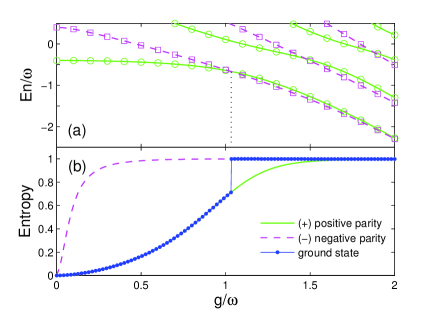
Figure 5: (color online) Energies (upper panel) and entanglement entropies (lower panel) of the ground state and the first excited state. A level crossing occurs at $g_{c}=4/\sqrt{15}$, marking a change of the parity of the ground state: $g<g_{c}$ the parity is positive (green-solid), and negative (purple-dashed) for $g>g_{c}$, as shown in upper panel. Correspondingly, we find that the ground state entropy displays a sharp discontinuity at the level crossing point, as shown in lower panel.

We remark that the ground states are degenerate at the level crossing point which is special.

V Discussion

In this article, we discussed a carefully chosen generalization of the Rabi model: The Hamiltonian system breaks the parity symmetry; the rotating and counter-rotating interactions are governed by two different coupling constants; a further parameter introduces a phase factor in the counter-rotating terms. We obtained exact energies and eigenstates of the system through the analytical properties of a transcendental function. We note that, because of the anisotropic coupling a peculiar phenomenon occurs in the energy spectrum of the system: the eigenstates belonging to different parity sectors swap in couples. We have quantified the crossing between the ground and the first excited state through the entanglement entropy of the spin system.

Our Hamiltonian systems capture the physics of notoriously important problems in different physical contexts, including two dimensional electron gas with general spin-orbit interaction, two level atom in electromagnetic field, and superconducting circuits in ultra-strong regimes. We explained how our results are immediately relevant for the experimental situations.

We believe that superconducting circuits made of two coupled SQUID’s could provide access to a systematic experimental study of the physical effects of the anisotropic Rabi interaction. Specifically, our study indicates that the circuit inductance, SQUID-SQUID inductance and the external magnetic field are the parameters that should be varied to study the crossover from the weak to strong coupling regimes (see Sect.III.2).

Acknowledgements. Q. T. X. and S. C. contributed equally. We thank useful discussions with B. Englert and Wei-Bin Yan. We thank X. B. Zhu for discussions about the experimental realization in superconducting flux qubit system. This work was supported by “973” program (2010CB922904), grants from NSFC and CAS.

Appendix A Exact solution of the anisotropic Rabi model

For the Hamiltonian presented in (1), the parameter $\lambda$ controls the anisotropy between the rotating and the counter rotating terms and $\theta$ introduce a phase into the counter rotating terms only; term $\epsilon\sigma_{x}$ breaks the $Z_{2}$ symmetry, and therefore the eigenspace of the model (1) cannot be split in invariant subspaces. Nevertheless, the model (1) can still be solved exactly with the approach originally developed by BraakBraak for the isotropic model $\lambda=1$, $\theta=\epsilon=0$.

In solving exactly this model, firstly, for technical convenience (we comment further below), we perform a unitary transformation $U(\lambda,\theta)$,

$$U(\lambda,\theta) = \left(\begin{array}[]{cc}\cos\eta e^{i\theta/2}&-\sin\eta\\ \sin\eta&\cos\eta e^{-i\theta/2}\end{array}\right)$$ (17)

$$= \frac{1}{\sqrt{1+\lambda}}\left(\begin{array}[]{cc}\xi&-\sqrt{\lambda}\\ \sqrt{\lambda}&\xi^{*}\end{array}\right),$$ (20)

where $\tan\eta=\sqrt{\lambda}$, $\xi=e^{i\theta/2}$, when $\theta=0$, $\xi=1$, it is a orthogonal transformation. The Hamiltonian (1) becomes

$$U^{\dagger}HU=\left(\begin{array}[]{cc}\omega a^{\dagger}a+\sqrt{\lambda}g(\xi^{*}a+\xi a^{\dagger})+c&\xi^{*2}(1-\lambda)ga-d^{*}\\ \xi^{2}(1-\lambda)ga^{\dagger}-d&\omega a^{\dagger}a-\sqrt{\lambda}g(\xi^{*}a+\xi a^{\dagger})-c\end{array}\right).$$ (21)

where $c=\frac{1-\lambda}{1+\lambda}\Delta+\frac{(\xi+\xi^{*})\sqrt{\lambda}}{1+\lambda}\epsilon$, $d=\frac{2\sqrt{\lambda}\xi}{1+\lambda}\Delta-\frac{\xi^{2}-\lambda}{1+\lambda}\epsilon$. We exploit the Bargmann representation of bosonic operators in terms of analytic functions: $a^{\dagger}\rightarrow z,a\rightarrow\frac{\partial}{\partial z}$, and consider the eigenfunction of the Hamiltonian as $(\phi_{1},\phi_{2})^{T}$, we have

$$\left[\omega z\frac{{\rm d}}{{\rm d}z}+\sqrt{\lambda}g(\xi^{*}\frac{{\rm d}}{{\rm d}z}+\xi z)+c\right]\phi_{1}+\left[\xi^{*2}(1-\lambda)g\frac{{\rm d}}{{\rm d}z}-d^{*}\right]\phi_{2} = E\phi_{1},$$ (22)

$$\left[\xi^{2}(1-\lambda)gz-d\right]\phi_{1}+\left[\omega z\frac{{\rm d}}{{\rm d}z}-\sqrt{\lambda}g(\xi^{*}\frac{{\rm d}}{{\rm d}z}+\xi z)-c\right]\phi_{2} = E\phi_{2}.$$ (23)

For convenience, we introduce the notations $\phi_{1,2}(z)=\exp(-\frac{\sqrt{\lambda}g\xi}{\omega}z)\psi_{1,2}(y)$, $y=z+\frac{\sqrt{\lambda}g\xi^{*}}{\omega}$, $x=E+\frac{\lambda g^{2}}{\omega}$, $f=d+\frac{(1-\lambda)\sqrt{\lambda}g^{2}\xi}{\omega}$. Now, we obtain,

$$(\omega y\frac{{\rm d}}{{\rm d}y}-x+c)\psi_{1}=\left[f^{*}-\xi^{*2}(1-\lambda)g\frac{{\rm d}}{{\rm d}y}\right]\psi_{2},$$ (24)

and

$$\left[(\omega y-2\sqrt{\lambda}g\xi^{*})\frac{{\rm d}}{{\rm d}y}-2\sqrt{\lambda}g\xi y+\frac{4\lambda g^{2}}{\omega}-x-c\right]\psi_{2}$$

$$~{}~{}~{}~{}~{}~{}~{}~{}~{}~{}~{}~{}~{}~{}~{}=\left[f-(1-\lambda)gy\right]\psi_{1}.$$ (25)

Assuming that the functions $\psi_{1,2}$ can be expanded as, $\psi_{2}=\sum_{n=0}^{\infty}K_{n}^{+}(x)y^{n}$, $\psi_{1}=\sum_{n=0}^{\infty}L_{n}^{+}(x)y^{n}$, from Eq. (24), the relation between $K_{n}^{+}$ and $L_{n}^{+}$ is found as

$$L_{n}^{+}=\frac{f^{*}K_{n}^{+}-\xi^{*2}(1-\lambda)gK_{n+1}^{+}(n+1)}{n\omega-x+c}.$$ (26)

Then from Eq.(25), the recursive relation of $K_{n}^{+}$ is obtained,

$$a_{n}(x)K_{n+1}^{+} = b_{n}(x)K_{n}^{+}+c_{n}(x)K_{n-1}^{+},$$ (27)

$$a_{n}(x) = \left[2\sqrt{\lambda}-\frac{(1-\lambda)f\xi^{*}}{n\omega-x+c}\right](n+1)g\xi^{*},$$ (28)

$$b_{n}(x) = \frac{4\lambda g^{2}}{\omega}+n\omega-x-c-\frac{f^{*}f}{n\omega-x+c}$$ (29)

$$-\frac{(1-\lambda)^{2}g^{2}n}{(n-1)\omega-x+c},$$

$$c_{n}(x) = -2\sqrt{\lambda}g\xi+\frac{(1-\lambda)gf^{*}\xi^{2}}{(n-1)\omega-x+c}.$$ (30)

where $K_{-1}^{+}=0,K_{0}^{+}=1$, $n=0,1,2,...$. Incidentally, we comment that the unitary transformation (20) is a key step leading to simplify the recursive relations which involve only three terms, as it is displayed above.

Consequently, one sets of solutions is obtained:

$$\phi_{1}(z) = \exp(-\frac{\sqrt{\lambda}g\xi}{\omega}z)\sum_{n=0}^{\infty}L_{n}^{+}(z+\frac{\sqrt{\lambda}g\xi^{*}}{\omega})^{n},$$ (31)

$$\phi_{2}(z) = \exp(-\frac{\sqrt{\lambda}g\xi}{\omega}z)\sum_{n=0}^{\infty}K_{n}^{+}(z+\frac{\sqrt{\lambda}g\xi^{*}}{\omega})^{n}.$$ (32)

Then, substituting $z\rightarrow-z$ in Eq.(22,23), $\phi_{1}(-z)=\overline{\phi}_{1}(z)$, $\phi_{2}(-z)=\overline{\phi}_{2}(z)$ are eigenfunctions of the spectral problem (23) as well. Such functions can be obtained by applying the same procedure led to (31) and (32). The differential equations for $\overline{\phi}_{1}(z)$ and $\overline{\phi}_{2}(z)$ are

$$\left[\omega z\frac{{\rm d}}{{\rm d}z}-\sqrt{\lambda}g(\xi^{*}\frac{{\rm d}}{{\rm d}z}+\xi z)+c\right]\overline{\phi}_{1}+$$

$$+\left[-\xi^{*2}(1-\lambda)g\frac{{\rm d}}{{\rm d}z}-d^{*}\right]\overline{\phi}_{2}=E\overline{\phi}_{1},$$ (33)

$$\left[-\xi^{2}(1-\lambda)gz-d\right]\overline{\phi}_{1}+$$

$$+\left[\omega z\frac{{\rm d}}{{\rm d}z}+\sqrt{\lambda}g(\xi^{*}\frac{{\rm d}}{{\rm d}z}+\xi z)-c\right]\overline{\phi}_{2}=E\overline{\phi}_{2}.$$ (34)

Using the following notations, $\overline{\phi}_{1,2}(z)=\exp(-\frac{\sqrt{\lambda}g\xi}{\omega}z)\overline{\psi}_{1,2}(y)$, $y=z+\frac{\sqrt{\lambda}g\xi^{*}}{\omega}$, $x=E+\frac{\lambda g^{2}}{\omega}$, $\overline{f}=d-\frac{(1-\lambda)\sqrt{\lambda}g^{2}\xi}{\omega}$, the above equations can be rewritten as,

$$\left[(\omega y-2\sqrt{\lambda}g\xi^{*})\frac{{\rm d}}{{\rm d}y}-2\sqrt{\lambda}g\xi y+\frac{4\lambda g^{2}}{\omega}-x+c\right]\overline{\psi}_{1}$$

$$=\left[\overline{f}^{*}+\xi^{*2}(1-\lambda)g\frac{{\rm d}}{{\rm d}y}\right]\overline{\psi}_{2},$$ (35)

$$(\omega y\frac{{\rm d}}{{\rm d}y}-x-c)\overline{\psi}_{2}=\left[\overline{f}+\xi^{2}(1-\lambda)gy\right]\overline{\psi}_{1}.$$ (36)

Expand functions $\overline{\psi}_{1,2}$ as $\overline{\psi}_{1}=\sum_{n=0}^{\infty}K_{n}^{-}(x)y^{n}$, $\overline{\psi}_{2}=\sum_{n=0}^{\infty}L_{n}^{-}(x)y^{n}$, from Eq.(36) we find the relation of $K_{n}^{-}$ and $L_{n}^{-}$,

$$L_{n}^{-}=\frac{\overline{f}K_{n}^{-}+\xi^{2}(1-\lambda)gK_{n-1}^{-}}{n\omega-x-c}$$ (37)

Then from Eq.(35) we obtain the recursive relation

$$\overline{a}_{n}(x)K_{n+1}^{-} = \overline{b}_{n}(x)K_{n}^{-}+\overline{c}_{n}(x)K_{n-1}^{-},$$ (38)

$$\overline{a}_{n}(x) = \left[2\sqrt{\lambda}+\frac{(1-\lambda)\overline{f}\xi^{*}}{(n+1)\omega-x-c}\right](n+1)g\xi^{*},$$

$$\overline{b}_{n}(x) = \frac{4\lambda g^{2}}{\omega}+n\omega-x+c-\frac{\overline{f}^{*}\overline{f}}{n\omega-x-c}$$ (40)

$$-\frac{(1-\lambda)^{2}g^{2}(n+1)}{(n+1)\omega-x-c},$$

$$\overline{c}_{n}(x) = -2\sqrt{\lambda}g\xi-\frac{(1-\lambda)g\overline{f}^{*}\xi^{2}}{n\omega-x-c}.$$ (41)

where $K_{-1}^{-}=0,K_{0}^{-}=1$, $n=0,1,2,...$

Going back to the original notations, we have,

$$\overline{\phi}_{1}(z) = \exp(-\frac{\sqrt{\lambda}g\xi}{\omega}z)\sum_{n=0}^{\infty}K_{n}^{-}(z+\frac{\sqrt{\lambda}g\xi^{*}}{\omega})^{n},$$ (42)

$$\overline{\phi}_{2}(z) = \exp(-\frac{\sqrt{\lambda}g\xi}{\omega}z)\sum_{n=0}^{\infty}L_{n}^{-}(z+\frac{\sqrt{\lambda}g\xi^{*}}{\omega})^{n}.$$ (43)

Considering the relation of these two sets of eigenstates mentioned above, $\phi_{1}(-z)=C\overline{\phi}_{1}(z)$, $\phi_{2}(-z)=C\overline{\phi}_{2}(z)$, then canceling the arbitrary constant $C$, a transcendental function can be constructed as,

$$G_{\epsilon}(x;z) = \phi_{1}\overline{\phi}_{2}-\phi_{2}\overline{\phi}_{1},$$ (44)

Because $G_{\epsilon}(x;z)$ is well defined at $z=\pm\sqrt{\lambda}g\xi^{*}/\omega$ within the convergent radius $R=2\sqrt{\lambda}g\xi^{*}/\omega$, we can set $z=0$ Braak . The function $G_{\epsilon}(x;0)$ is analytic in the complex plane except in the simple poles

$$x^{pole}_{n} = n\omega-\frac{(1-\lambda)^{2}g^{2}}{2\omega}+\frac{(\xi+\lambda\xi^{*})\epsilon}{2\sqrt{\lambda}},$$ (45)

$$\overline{x}_{n}^{pole} = (n+1)\omega-\frac{(1-\lambda)^{2}g^{2}}{2\omega}-\frac{(\xi+\lambda\xi^{*})\epsilon}{2\sqrt{\lambda}},$$ (46)

which follows from the zeros of the denominator of $K_{n}^{\pm}$: $a_{n}(x)=0$ and $\overline{a}_{n}(x)=0$ in Eq.(27) and Eq.(38), respectively. Then, the eigenvalues and eigenstates can be obtained by solving $G_{\epsilon}(x)=0$,

$$E_{n} = x_{n}-\frac{\lambda g^{2}}{\omega},$$ (47)

$$\Psi_{n} = U(\lambda,\theta)\left(\begin{array}[]{cc}\phi_{1}(x_{n})\\ \phi_{2}(x_{n})\end{array}\right)$$ (50)

$$= U(\lambda,\theta)\left(\begin{array}[]{cc}\sum_{n=0}^{\infty}L_{n}^{+}|n\rangle\rangle\\ \sum_{n=0}^{\infty}K_{n}^{+}|n\rangle\rangle\end{array}\right),$$ (53)

Using the second solution, the eigenstates of Hamiltonian with $a\rightarrow-a$, $a^{\dagger}\rightarrow-a^{\dagger}$ can be obtained:

$$\overline{\Psi}_{n} = U(\lambda,\theta)\left(\begin{array}[]{cc}\overline{\phi}_{1}(x_{n})\\ \overline{\phi}_{2}(x_{n})\end{array}\right)$$ (56)

$$= U(\lambda,\theta)\left(\begin{array}[]{cc}\sum_{n=0}^{\infty}K_{n}^{-}|n\rangle\rangle\\ \sum_{n=0}^{\infty}L_{n}^{-}|n\rangle\rangle\end{array}\right),$$ (59)

where

$$|n\rangle\rangle\doteq(a^{\dagger}+\frac{\sqrt{\lambda}g\xi^{*}}{\omega})^{n}|-\frac{\sqrt{\lambda}g\xi}{\omega}\rangle,$$

$$|-\frac{\sqrt{\lambda}g\xi}{\omega}\rangle=e^{-\frac{\lambda g^{2}}{2\omega^{2}}-\frac{\sqrt{\lambda}g\xi}{\omega}a^{\dagger}}|0\rangle.$$ (60)

In case $\lambda=1$ and $\theta=0$, we can recover the results given by Braak Braak and some generalized results Chen ; Tomka ; Albert2012 . Some other detailed calculations can be found in appendix.

Appendix B results for $Z_{2}$ symmetric case

For $\epsilon=0$, the anisotropic Rabi model enjoys a $Z_{2}$ symmetry reflecting the conservation of the parity of the operator

$$\hat{N}=a^{\dagger}a+\frac{1}{2}(\sigma_{z}+1),$$ (61)

In this case, the phase factors $e^{\pm i\theta}$ in the Hamiltonian can be canceled by a unitary transformation $R(\theta)$,

$$R(\theta)=e^{i\frac{\theta}{2}(\hat{N}-\frac{1}{2})}=e^{i\frac{\theta}{2}(\frac{\sigma_{z}}{2}+a^{\dagger}a)},$$ (62)

$$R^{\dagger}(\theta)HR(\theta) = \omega a^{\dagger}a+\Delta\sigma_{z}+g[\sigma^{+}a+\sigma^{-}a^{\dagger}$$ (63)

$$+\lambda(\sigma^{+}a^{\dagger}+\sigma^{-}a)].$$

Therefore the parameter $\theta$ gives no contribution to the energy spectra, but enters the wave functions only.

We shall see that the $Z_{2}$ symmetry effectively simplifies the procedure of finding the exact spectrum since the transcendental function $G_{\epsilon}(x)$, $\epsilon=0$, can be discussed into the different parity sectors separately.

To simplify the solution of the spectral problem, we resort to a similar trick we employed above. Namely, we apply the rotation

$$V = U^{\dagger}(\lambda,\theta)W$$ (66)

$$= \frac{1}{\sqrt{2(1+\lambda)}}\left(\begin{array}[]{cc}\xi^{*}+\sqrt{\lambda}&-\xi^{*}+\sqrt{\lambda}\\ \xi-\sqrt{\lambda}&\xi+\sqrt{\lambda}\end{array}\right).$$

with

$$W=\frac{1}{\sqrt{2}}\left(\begin{array}[]{cc}1&-1\\ 1&1\end{array}\right).$$ (67)

to the Hamiltonian (63). Now, we have the Hamiltonian,

$$W^{\dagger}HW=\left(\begin{array}[]{cc}\omega a^{\dagger}a+\frac{1+\lambda}{2}(a+a^{\dagger})&\frac{1-\lambda}{2}(a-a^{\dagger})+\Delta\\ -\frac{1-\lambda}{2}(a-a^{\dagger})+\Delta&\omega a^{\dagger}a-\frac{1+\lambda}{2}(a+a^{\dagger})\end{array}\right).$$ (70)

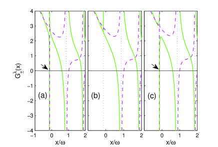
Figure 6: (color online) Comparison of transcendental functions near ground state degenerate point. From left to right, the parameters are (a) $g=g_{c}-0.01$, (b) $g=g_{c}$, (c) $g=g_{c}+0.01$, where $g_{c}=4/\sqrt{15}$ which is the degenerate point. $G_{+}^{\lambda}(x)$ (green-solid line) and $G_{-}^{\lambda}(x)$ (purple-dashed line) are presented as functions of $x$, where $\omega=1$, $\Delta=0.4$, $\lambda=0.5$, $\theta=0$. The difference of (a,b,c) can be observed, for example, at the points marked by arrows in the figures. For (a) at the point marked by arrow, the energy of positive parity is slightly less than the energy of negative parity, it is reversed in (c), while in (b), the pole is lifted since $K_{1}=0$.

The eigenfunctions $\phi_{1},\phi_{2}$ (and similarly $\overline{\phi}_{1},\overline{\phi}_{2}$) in the main text transform according to $(\varphi_{1},\varphi_{2})^{T}=V^{\dagger}(\phi_{1},\phi_{2})^{T}$:

$$\varphi_{1} = \frac{(\xi+\sqrt{\lambda})\phi_{1}+(\xi^{*}-\sqrt{\lambda})\phi_{2}}{\sqrt{2(1+\lambda)}},$$ (71)

$$\varphi_{2} = \frac{(-\xi+\sqrt{\lambda})\phi_{1}+(\xi^{*}+\sqrt{\lambda})\phi_{2}}{\sqrt{2(1+\lambda)}}.$$ (72)

We know that $\phi_{1},\phi_{2}$ read as,

$$\phi_{1}(z) = \exp(-\frac{\sqrt{\lambda}g\xi}{\omega}z)\sum_{n=0}^{\infty}L_{n}(x)(z+\frac{\sqrt{\lambda}g\xi^{*}}{\omega})^{n},$$

$$\phi_{2}(z) = \exp(-\frac{\sqrt{\lambda}g\xi}{\omega}z)\sum_{n=0}^{\infty}K_{n}(x)(z+\frac{\sqrt{\lambda}g\xi^{*}}{\omega})^{n},$$

where

$$L_{n} = \frac{f^{*}K_{n}-\xi^{*2}(1-\lambda)gK_{n+1}(n+1)}{n\omega-x+c}.$$ (74)

Here, the superindices $+$ are omitted.

The $Z_{2}$ symmetry reflects into a symmetry in the eigenfunction: $\varphi_{2}(-z)=C\varphi_{1}(z)$, where $C$ is an arbitrary constant. Without loss of generality we take $\varphi_{1,2}$ normalized and real. In this case, $C=\pm 1$, and the transcendental function $G$ is

$$G^{\lambda}_{\pm}(x;z)=\varphi_{2}(-z)\mp\varphi_{1}(z)=0\qquad\forall\ z\in{\cal C}$$ (75)

Setting $z=0$ as the above section, and substituting $\varphi_{1,2}$ by $\phi_{1,2}$,

$$G^{\lambda}_{+}(x) = -\xi\phi_{1}+\sqrt{\lambda}\phi_{2},$$

$$G^{\lambda}_{-}(x) = \sqrt{\lambda}\phi_{1}+\xi^{*}\phi_{2}.$$ (76)

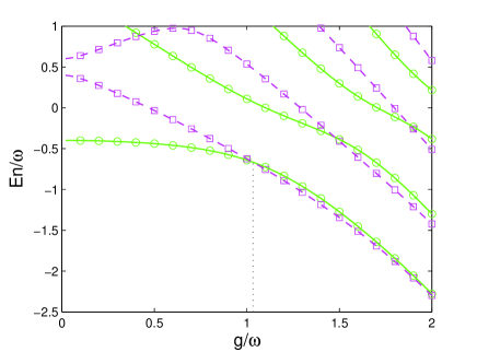
Figure 7: (color online) Ground state level crossing. The ground state energy and the first excited state energy are crossed for anisotropic Rabi model with $Z_{2}$ symmetry. The parity of the ground state changes when passing through the crossing point. Here $\epsilon=0$ for keeping $Z_{2}$ symmetry, we choose $\Delta=0.4,\lambda=0.5$, so $g=\frac{4}{\sqrt{15}},E_{0}^{e}=-\frac{2}{3}$ due to equations (12,11). The green-solid lines are for positive parity, the purple-dashed lines are for negative parity. The circles and blocks are numerical data, they agree well with analytical results shown in lines. Part of this figure is shown in the upper panel of FIG.5.

The energy spectrum can be divided into two cases. One case is the regular solution which is solely determined by zeros of the transcendental function. Another case corresponds to the exceptional solutions. For this case, we can consider first the the poles of the transcendental function determined by setting $a_{n}(x)=0$,

$$x_{n}^{pole}=n\omega-\frac{(1-\lambda)^{2}g^{2}}{2\omega}.$$ (77)

At the same time, if $K_{n+1}(x_{n}^{pole})=0$ for special values of the parameters $g$ and $\Delta$, the poles can be lifted, because the numerator of $G_{\pm}^{\lambda}$ is also vanishing. FIG. 6 shows the transition between regular solutions to exceptional solutions. This special solutions are Judd type solutions for the anisotropic Rabi model, corresponding to the so called isolated integrability Judd . Owing to $G_{\pm}^{\lambda}\neq 0$, these eigenvalues have no definite parity, and a double degeneracy of the eigenvalues occurs (see FIG. 3(b) in main text). In this case, the infinite series solutions $K_{n}$ and $L_{n}$ can be terminated as finite series solutions. We note that, in particular, there is no crossing with the same parity. Incidentally, a crossing between the ground state and the first excited state occurs for the anisotropic case which corresponds to the exact solutions obtained by Judd Judd , as already shown in Section IV.

FIG. 7 shows that the parity of the ground state changes sign when passing through the level crossing point. When $g/\omega$ is small, the ground state is positive parity, the first excited state is negative parity; after passing through the crossing point where the parity changes sign, the ground state is negative parity and the first excited state is positive parity. This parity changing can be demonstrated by the intrinsic symmetries of the ground state.

The ground state of Hamiltonian (1) with vanishing $\epsilon$ can be written as,

$$\Psi(z)=\left(\begin{array}[]{c}\varphi_{1}(z)\\ \varphi_{2}(z)\end{array}\right),$$ (80)

or $\varphi_{1}(z)\rightarrow\varphi_{2}(-z)$, $\varphi_{2}(z)\rightarrow\varphi_{1}(-z)$ since of the $Z_{2}$ symmetry. Additionally when $g/\omega$ is small which is less than the crossing point value, the ground state is parity positive and can be simplified as,

$$\Psi_{+}(z)=\left(\begin{array}[]{c}\varphi_{1}(z)\\ \varphi_{1}(-z)\end{array}\right).$$ (83)

In comparison, when $g/\omega$ is larger than the crossing point value, the ground state is parity negative and takes the form

$$\Psi_{-}(z)=\left(\begin{array}[]{c}\varphi_{1}(z)\\ -\varphi_{1}(-z)\end{array}\right).$$ (86)

However, we find that both $\Psi_{\pm}(z)$ are not the eigenstates of the Hamiltonian at the ground state level crossing point.

We may reformulate the ground state with different parities as

$$\Psi_{+}(z)=\left(\begin{array}[]{c}\varphi_{1}(z)+\varphi_{2}(-z)\\ \varphi_{2}(z)+\varphi_{1}(-z)\end{array}\right),$$ (89)

$$\Psi_{-}(z)=\left(\begin{array}[]{c}\varphi_{1}(z)-\varphi_{2}(-z)\\ \varphi_{2}(z)-\varphi_{1}(-z)\end{array}\right).$$ (92)

Those two states are the ground state and the first excited state. They are the correct eigenstates corresponding to different parities in the whole region including the level crossing point. Explicitly, one may confirm that $\Psi_{\pm}(z)$ in (89,92) are similar as the results in (83,86) when $g/\omega$ is not at the crossing point, respectively. The ground energy degeneracy at the crossing point also implies that arbitrary linear combinations of states $\Psi_{+}(z)$ and $\Psi_{-}(z)$ in (89,92) are also the ground state eigenstates.

With the help of the solutions (13,14), and also considering the transformation (67), the eigenstates at the level crossing point can be written as follows, up to a whole factor,

$$W\Psi_{+}(z)=\left(\begin{array}[]{c}\sqrt{\lambda}(\exp(-\frac{\sqrt{\lambda}g\xi}{\omega}z)-\exp(\frac{\sqrt{\lambda}g\xi}{\omega}z))\\ \xi^{\dagger}(\exp(-\frac{\sqrt{\lambda}g\xi}{\omega}z)+\exp(\frac{\sqrt{\lambda}g\xi}{\omega}z))\end{array}\right),$$ (95)

$$W\Psi_{+}(z)=\left(\begin{array}[]{c}\sqrt{\lambda}(\exp(-\frac{\sqrt{\lambda}g\xi}{\omega}z)+\exp(\frac{\sqrt{\lambda}g\xi}{\omega}z))\\ \xi^{\dagger}(\exp(-\frac{\sqrt{\lambda}g\xi}{\omega}z)-\exp(\frac{\sqrt{\lambda}g\xi}{\omega}z))\end{array}\right).$$ (98)

We remark that because of the ground states energy degeneracy, the linear combinations of the ground states may lead to simpler solutions,

$$\Psi(z)=\left(\begin{array}[]{c}\sqrt{\lambda}\exp(-\frac{\sqrt{\lambda}g}{\omega}z)\\ \exp(-\frac{\sqrt{\lambda}g}{\omega}z)\end{array}\right);~{}\left(\begin{array}[]{c}\sqrt{\lambda}\exp(\frac{\sqrt{\lambda}g}{\omega}z)\\ -\exp(\frac{\sqrt{\lambda}g}{\omega}z)\end{array}\right).$$ (103)

It can be checked that these are eigenstates of the Hamiltonian (1) for vanishing $\epsilon=0$ and $\theta=0$, with degeneracy conditions (12,11).

Finally, we remark that the Bargmann representation of bosonic operator used in our model can also be used in the JC mdoel, which has $U(1)$ symmetry. The eigenvalues and eigenstates can be obtained in the familiar steps, but simpler because the total number $\hat{N}=a^{\dagger}a+\frac{1}{2}(\sigma_{z}+1)$ is conserved.

B.1 Fitting with experimental data for the superconducting circuits in the strongly coupled regime

We consider the energy gaps between the anisotropic Rabi model and the JC model. Such energy differences, generalizing the Bloch-Siegert effect of the isotropic Rabi model, play important roles in many physical applications where the strong coupling regime is the actual one, like in the superconducting circuits and some similar physical systems Mooij1999 ; Gunter ; Wallraff ; Schuster ; Peropadre ; Nakamura .

Ordinarily, there is no general form for the gap, but we can analyze it at the degenerate points. The ground state energy of the JC model is $E_{0}^{JC}=-\Delta$, so the ground state gap at $|\Delta|=(1-\lambda^{2})g^{2}/2\omega$ is,

$$\Delta E_{0}=-\Delta-E_{0}^{e}=\frac{\lambda^{2}g^{2}}{\omega}.$$ (104)

when $\lambda=0$ (the JC limit), the gap vanishes; for $\lambda=1$, the gap is just the standard Bloch-Siegert shift in the Rabi model, $\Delta E_{0}={g^{2}}/{\omega}$. For $\lambda\neq 1$, the first excited state energy gap with the JC is

$$\Delta E_{1}=\frac{\omega}{2}-\sqrt{(\Delta-\frac{\omega}{2})^{2}+g^{2}}+\frac{(1+\lambda^{2})g^{2}}{2\omega}.$$ (105)

For small $g/\omega$, $\Delta E_{1}\approx\lambda^{2}g^{4}/\omega^{3}$, remarkably different from the standard Bloch-Siegert shift ${g^{2}}/{\omega}$. This is for case $|\Delta|=(1-\lambda^{2})g^{2}/2\omega$, as we just mentioned.

In the Rabi model, there is a crossing between the second and the third energy levels at $|\Delta|=\sqrt{\omega^{2}-4g^{2}}$, $E=\omega-g^{2}/\omega$ Braak , the second energy level of the JC model in small $g/\omega$ can be written as

$$E_{2}^{JC} = \frac{\omega}{2}+\sqrt{(\Delta-\frac{\omega}{2})^{2}+g^{2}}$$ (106)

$$\approx \omega-\frac{g^{2}}{\omega}+\frac{g^{4}}{\omega^{3}}.$$

Obviously, the second excited energy difference between the JC model and Rabi model is in $g^{4}/\omega^{3}$ scale, too. However, we compare the third excited energy difference at this point as

$$E_{3}^{JC}-E_{1}^{e,Rabi} = \frac{3\omega}{2}-\sqrt{(\Delta-\frac{\omega}{2})^{2}+2g^{2}}-(\omega-\frac{g^{2}}{\omega})$$ (107)

$$\approx \frac{g^{2}}{\omega}-\frac{2g^{4}}{\omega^{3}}.$$

where the condition $g/\omega\ll 1$ is used, the difference is still in $g^{2}/\omega$ scale. Maybe the energy differences of the second and third excited state are strange at the degenerate point. Those differences may be verified by the recent experiments with ultrastrong coupling.

In ultrastrong coupling regime, the deviation from the JC model known as Bloch-Siegert shift was experimentally observedMooij , which is an LC resonator magnetically coupled to a superconducting flux qubit in the ultrastrong coupling regime, and the system can be modeled by the Hamiltonian,

$$H^{\prime} = \frac{\omega_{q}}{2}(\sigma_{z}+1)+\omega_{r}a^{\dagger}a$$ (108)

$$+g(\cos\vartheta\sigma_{z}-\sin\vartheta\sigma_{x})(a+a^{\dagger}),$$

with $\omega_{q}\equiv\sqrt{\epsilon^{2}+\Delta^{2}}$, $\epsilon=2\pi I_{p}(\Phi-\Phi_{0}/2)$ and $\tan\vartheta=\Delta/\epsilon$, where $\hbar$ is conventionally set to 1.

Following results shown in Ref.Mooij , if we neglect the term $g\cos\vartheta\sigma_{z}(a+a^{\dagger})$, which only contributes a constant $-g^{2}\cos^{2}\vartheta/\omega_{r}$ to the second order under the transformation $U=\exp(-g\cos\vartheta/\omega_{r}\sigma_{z}(a-a^{\dagger}))$. And by omitting the counter-rotating term, the corresponding JC model is given by

$$H_{JC}=\frac{\omega_{q}}{2}(\sigma_{z}+1)+\omega_{r}a^{\dagger}a-g\sin\vartheta(\sigma^{-}a^{\dagger}+\sigma^{+}a).$$

(109)

In the ultrastrong coupling regime, the rotating wave approximation is thus inappropriate, the experimental results of this system will not agree with the JC model. The Bloch-Siegert shift caused by the counter-rotating term is evidently observed.

Then, we directly use our proposed anisotropic model to fit this system

$$H_{a-Rabi} = \frac{\omega_{q}}{2}(\sigma_{z}+1)+\omega_{r}a^{\dagger}a$$

$$-g\sin\vartheta(\sigma^{-}a^{\dagger}+\sigma^{+}a+\lambda(\sigma^{-}a+\sigma^{+}a^{\dagger})).$$

where the anisotropic parameter $\lambda$ is decided by fitting, and $g=0.74$GHz, $\Delta=4.21$GHz, $I_{p}=500$nA, $\omega_{r}=8.13$GHz, are the same as previous obtained Mooij . As shown in Fig. 4, we can find that the experimental data agree perfectly with the case $\lambda=0.5$ (red dashed dot line) which is neither the Rabi model nor the JC model, and we remark that the result of $\lambda=0.7$ case seems similar as the Hamiltonian (108) (solid black line), and $\lambda=0$ case is the same as the JC Hamiltonian (109) (dashed black line). Here we try to comment that by this experimental set up, the anisotropic Rabi model may be tested in a full regime by using qubit devices with strength of coupling ranging from weak to ultrastrong up to $g\approx 2$GHz within current technologies.

References

- (1) I. I. Rabi, Space Quantization in a Gyrating Magnetic Field, Phys. Rev. 51, 652-654 (1937).
- (2) M. O. Scully and M. S. Zubairy, Quantum optics (Cambridge University Press, Cambridge, 1997).
- (3) M. Wagner, Unitary Transformations in Solid State Physics (North-Holland, Amsterdam, 1986).
- (4) E. T. Jaynes and W. W. Cummings, Comparison of quantum and semiclassical radiation theories with application to the beam maser, Proc. IEEE 51, 89 (1963).
- (5) J. M. Raimond, M. Brune, and S. Haroche, Manipulating quantum entanglement with atoms and photons in a cavity, Rev. Mod. Phys. 73, 565-582 (2001).
- (6) D. Liebfried, R. Blatt, C. Monroe, and D. Wineland, Quantum dynamics of single trapped ions, Rev. Mod. Phys. 75, 281-324 (2003).
- (7) D. Englund et. al., Controlling cavity reflectivity with a single quantum dot, Nature 450, 857-861 (2007).
- (8) E. K. Irish, Generalized Rotating-Wave Approximation for Arbitrarily Large Coupling, Phys. Rev. Lett. 99, 173601 (2007).
- (9) L. Amico, H. Frahm, A. Osterloh, and G. A. P. Ribeiro, Integrable spin-boson models descending from rational six-vertex models, Nucl. Phys. B 787, 283-300 (2007).
- (10) D. Braak, Integrability of the Rabi model, Phys. Rev. Lett. 107, 100401 (2011).
- (11) B. R. Judd, Exact solutions to a class of Jahn-Teller systems, J. Phys. C 12, 1685 (1979).
- (12) F. Bloch and A. Siegert, Magnetic resonance for nonrotating fields, Phys. Rev. 57, 522 (1940).
- (13) J. H. Shirley, Solution of the Schrödinger Equation with a Hamiltonian Periodic in Time, Phys. Rev. B 138, 979 (1965).
- (14) D. Esteve, Superconducting qubits, in Proceedings of the Les Houches 2003 Summer School on Quantum Entanglement and Information Processing, (D. Esteve and J.-M. Raimond, editors), Elsevier (2004).
- (15) I. Chiorescu et al., Coherent dynamics of a flux qubit coupled to a harmonic oscillator, Nature 431, 159-162 (2004);
- (16) K. V. R. M. Murali et al., Probing Decoherence with Electromagnetically Induced Transparency in Superconductive Quantum Circuits, Phys. Rev. Lett. 93 087003 (2004).
- (17) L. Amico and K. Hikami, Integrable spin-boson interaction in the Tavis-Cummings model from a general boundary twist, Eur. Phys. J. B 43, 387 (2005).
- (18) P. Forn-Diaz et al., Observation of the Bloch-Siegert shift in a qubit-oscillator system in the ultrastrong coupling regime, Phys. Rev. Lett. 105, 237001 (2010).
- (19) T. Niemczyk et al., Circuit quantum electrodynamics in the ultrastrong-coupling regime, Nature Physics 6, 772 (2010).
- (20) J. Tuorila et al., Stark effect and generalized Bloch-Siegert shift in a strongly driven two-level system, Phys. Rev. Lett. 105, 257003 (2010).
- (21) M. Z. Hasan and C. L. Kane, Colloquium: Topological insulators, Rev. Mod. Phys. 82, 3045-3067 (2010).
- (22) Y. K. Kato, R. C. Myers, A. C. Gossard, and D. D. Awschalom, Observation of the Spin Hall Effect in Semiconductors, Science 306, 1910-1913 (2004).
- (23) S. Datta and B. Das, Electronic analog of the electro- optic modulator, Appl. Phys. Lett. 56, 665 (1990).
- (24) E.I. Rashba, Properties of semiconductors with an extremum loop .1. Cyclotron and combinational resonance in a magnetic field perpendicular to the plane of the loop, Sov. Phys. Solid State 2, 1109 (1960).
- (25) G. Dresselhaus, Spin-orbit coupling effects in Zinc Blende Structures, Phys. Rev. 100, 580 (1955).
- (26) J. Schliemann, J. Carlos Egues and D. Loss, Variational study at the quantum Hall ferromagnet in the presense of spin-orbit interaction, Phys. Rev. B 67, 085302 (2003).
- (27) L. W. Molenkamp, G. Schmidt, and G. E. W. Bauer, Rashba Hamiltonian and electron transport, Phys. Rev. B 64, 121202 (2001).
- (28) Y. J. Lin, K. Jiménez-García, and I. B. Spielman, Spin-orbit-coupled Bose-Einstein condensates, Nature 471, 83-87 (2011).
- (29) X. J. Liu, M. F. Borunda, X. Liu, and J. Sinova, Effect of Induced Spin-Orbit Coupling for Atoms via Laser Fields, Phys. Rev. Lett. 102, 046402 (2009).
- (30) C. J. Kennedy, G. A. Siviloglou, H. Miyake, W. C. Burton, and W. Ketterle, Spin-orbit coupling and spin Hall effect for neutral atoms without spin-flips, eprint arXiv:1308.6349.
- (31) I. Bloch, J. Balibard, and S. Nascimbène, Quantum simulations with ultracold quantum gases, Nature Physics 8, 267-276 (2012).
- (32) V. V. Albert, Quantum Rabi Model for N-State Atoms, Phys. Rev. Lett. 108, 180401 (2012).
- (33) Q. H. Chen et al., Exact solvability of the quantum Rabi model using Bogoliubov operators, Phys. Rev. A 86, 023822 (2012).
- (34) M. Tomka, O. El Araby, M. Pletyukhov, V. Gritsev, Exceptional and regular spectra of the generalized Rabi model, eprint arXiv:1307.7876.
- (35) J. E. Mooij et al., Josephson Persistent-Current Qubit, Science 285, 1036-1039 (1999).
- (36) G. Günter et al., Sub-cycle switch-on of ultrastrong light-matter interaction, Nature 458, 178-181 (2009).
- (37) A. Waltraff et al., Strong coupling of a single photo to a superconducting qubit using circuit quantum electrodynamics, Nature 431, 162-167 (2004).
- (38) D. I. Schuster et al., Resolving photon number states in a superconducting circuit, Nature 445, 515 (2007).
- (39) B. Peropadre, P. Forn-Díaz, E. Solano, and J. J. García-Ripoll, Switchable Ultrastrong Coupling in Circuit QED, Phys. Rev. Lett. 105, 023601 (2010).
- (40) Y. Nakamura, Yu. A. Pashkin, and J. S. Tsai, Rabi Oscillations in a Josephson-Junction Charge Two-Level System, Phys. Rev. Lett. 87, 246601 (2001).
- (41) X. B. Zhu et al., Coherent coupling of a superconducting flux qubit to an electron spin ensemble in diamond, Nature 478, 221 (2011).
- (42) L. Amico, R. Fazio, A. Osterloh, and V. Vedral, Entanglement in many-body systems, Rev. Mod. Phys. 80, 517 (2008).
- (43) J. Eisert, M. Cramer, M.B. Plenio, Rev. Mod. Phys. 82, 277 (2010).