Tunable interactions between paramagnetic colloidal particles driven in a modulated ratchet potential^‡

Arthur V. Straube^a and Pietro Tierno^∗b,c

We study experimentally and theoretically the interactions between paramagnetic particles dispersed in water and driven above the surface of a stripe patterned magnetic garnet film. An external rotating magnetic field modulates the stray field of the garnet film and generates a translating potential landscape which induces directed particle motion. By varying the ellipticity of the rotating field, we tune the inter-particle interactions from net attractive to net repulsive. For attractive interactions, we show that pairs of particles can approach each other and form stable doublets which afterwards travel along the modulated landscape at a constant mean speed. We measure the strength of the attractive force between the moving particles and propose an analytically tractable model that explains the observations and is in quantitative agreement with experiment.

1 Introduction

The transport of particles due to a ratchet mechanism ¹ is a general phenomenon arising in many branches of physics, and biology. ^{2, 3, 4} Ratchet effects are found in Abrikosov vortices, ⁵ and Josephson vortices in superconductors, ⁶ electrons in semiconductor heterostructures, ⁷ cold atoms, ⁸ ferrofluids ⁹ and granular materials ¹⁰ to name a few examples. In biological systems, ratchet effects are also found in molecular motors such as myosin ^{11, 12, 13} or actin. ^{14, 15, 16}

Single particles, molecules or proteins, when placed in an asymmetric potential will undergo a net transport under non-equilibrium fluctuations. However, when considering an ensemble of interacting species, the system transport properties are often dictated by a delicate balance between the particle interactions and the rectification process above the asymmetric potential. Unlike molecular machines, or quasi-particles in quantum systems, colloidal particles are characterized by experimentally accessible time and length scales, and these features promote their use as a model system to investigate the emergence of novel ratchet effects. ^{17, 18, 19, 20, 21} In addition, in colloidal systems forces and potentials between the individual particles can be directly measured via particle tracking techniques. ^{22, 23}

When colloidal particles can be polarized, like paramagnetic colloids, external fields can be used to induce dipolar interactions, and assemble these particles into compact structures such us doublets, ²⁴ chains ²⁵ or clusters. ²⁶ Magnetic substrates with features on the colloidal length scale, have been recently used to induce directed ratchet transport of paramagnetic colloidal particles. ^{27, 28} However, most of the recent works concerned the transport of magneticcolloidal particles focused mainly on the dynamic properties of individual particles or collective ensembles, but not on measuring the interaction forces between the transported particles. On the other hand, theoretical works that studied interacting pairs of particles exhibiting a ratchet-like transport showed the richness of the physical system. ^{29, 30, 31}

In addition, the use of magnetic fields gives the freedom to induce attractive or repulsive interactions via dipolar forces. Thus, the competition between dipolar forces,

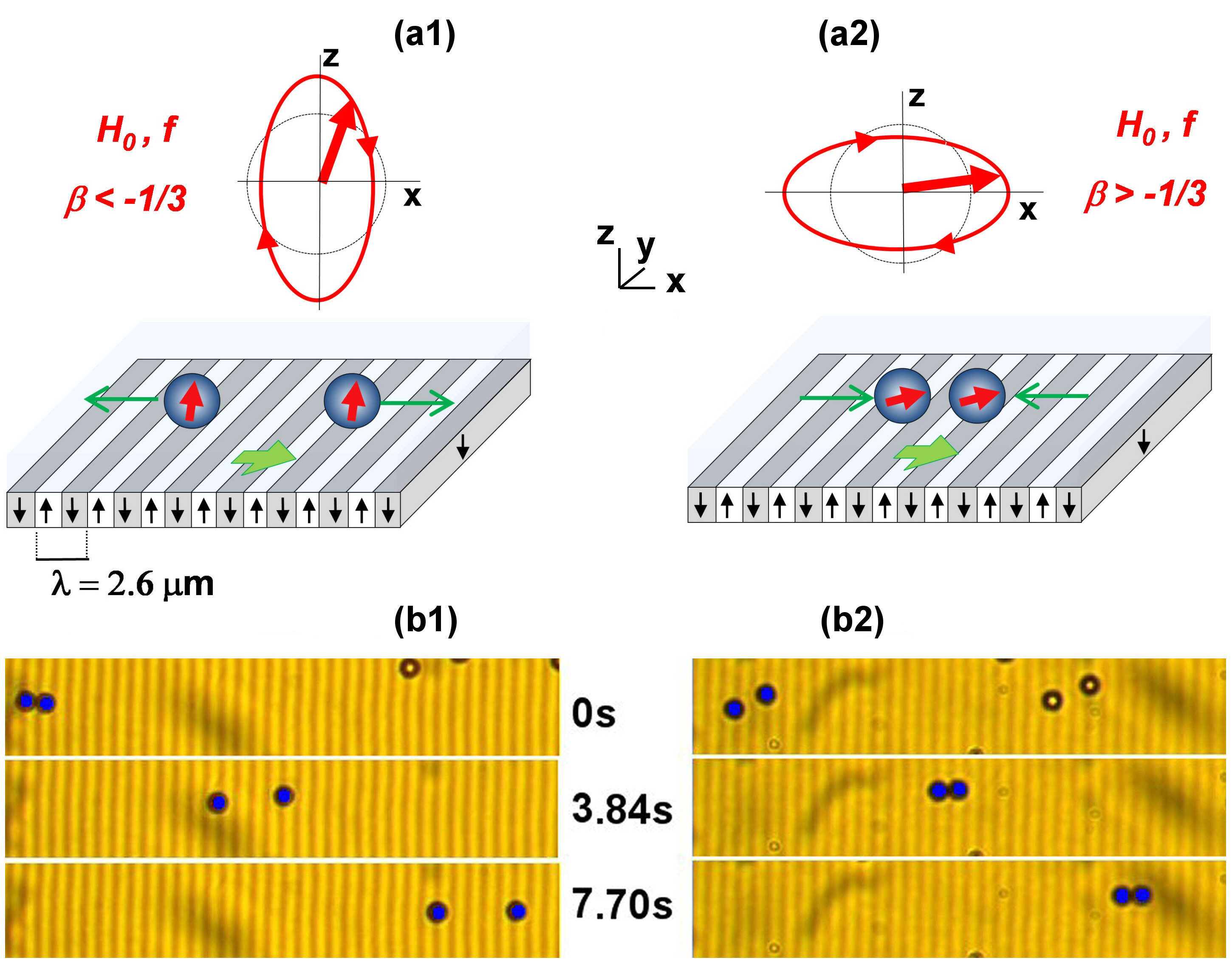
Fig.  1: (a1,a2) Schematic illustrations of a pair of paramagnetic particles transported above the ferrite garnet film (FGF). The particles display either repulsive (a1) or attractive (a2) interactions induced by a rotating magnetic field with elliptic polarization. The field is characterized by a frequency $f$, amplitude $H_{0}$ and ellipticity parameter $\beta<\beta_{\rm c}$ (a1) or $\beta>\beta_{\rm c}$ (a2); for particles having no relative displacement along the stripes, $\beta_{c}=-1/3$. (b1,b2) Series of optical microscope images at consequent instant showing a pair of particles (highlighted in blue) driven above the FGF and subjected to a magnetic field with $f=10\,{\rm Hz}$, $H_{0}=730\,{\rm A/m}$ and $\beta=-0.6$ (b1), $\beta=0.6$ (b2).

which align the particles, and the substrate field which transports them, could give rise to novel colloidal structures and dynamics phases. ^{32, 33, 34, 35}

In this article, we present a detailed study of the interactions between pairs of paramagnetic particles driven in a periodic potential via a deterministic ratchet effect. The latter is realized by externally modulating the magnetic stray field generated at the surface of a ferrite garnet film (FGF). The modulation corresponding to the rotation of the field breaks the symmetry and induces a net particle transport above the FGF. The elliptic polarization of the rotating field is used to tune the inter-particle interactions from net attractive to net repulsive effects. The experimental situations considered are schematically depicted in Fig. 1(a1,a2). When the ellipticity of the field is such that repulsive interactions dominate (a1), the paramagnetic colloidal particles either stay disperse, or couple into oscillating pairs which move above the film. In the opposite situation, when the field ellipticity forces the particles to attract each other (a2), moving particles approach till forming stable doublets. Afterwards, such doublets propel above the FGF at a constant mean speed. We apply a theoretical model that accounts for magnetic dipolar interactions between the particles driven across the stripes. By integrating out the fast oscillatory motion caused by the temporal modulation, we put forward an analytically tractable model describing the dynamics at slow time scales. The theoretical predictions drawn from this model explain the pair interactions and are in good quantitative agreement with experiment.

2 Experimental system

In the experiments, we use a monodisperse suspension of paramagnetic colloidal particles (Dynabeads M-270, Dynal) with radius $a=1.4\,{\rm\mu m}$ and magnetic volume susceptibility $\chi\sim 1$.³⁶ The particles were originally dispersed in purified water at a concentration of $\sim 2\times 10^{9}$ beads/ml. We dilute the stock solution with high deionized water (MilliQ system, $18.2\,{\rm M\Omega\,\,cm}$) up to a concentration of $\sim 3\times 10^{9}$ beads/ml and deposit a drop of it on top of the ferromagnetic domains of an uniaxial ferrite garnet film (FGF). The FGF film was grown by dipping liquid phase epithaxy on a gadolinium gallium garnet (GGG) substrate. ³⁷ The FGF was characterized by a series of parallel stripe domains with opposite magnetization and spatial periodicity $\lambda=2.6\,{\rm\mu m}$, which is twice the domain width, Fig. 1(a). Between opposite magnetized domains there are Bloch walls (BWs), i.e. are narrow transition regions ($\sim 20\,{\rm nm}$) where the magnetization rotates, and thus the stray field of the film is maximal.

After deposition of the droplet, it takes the particles few minutes to sediment above the film and get pinned above the BWs. To prevent particle adhesion to the magnetic substrate due to the strong attraction of the BWs, the FGF was coated with a $1{\rm\mu m}$ thick layer of a photoresist AZ-1512 (Microchem, Newton, MA) following a protocol detailed in a previous work. ³⁸ The polymer film also reduced the strong attraction of the BWs, since the stray field of the FGF decreases exponentially with the elevation. ³⁹

The external rotating magnetic field elliptically polarized in the $(x,z)$ plane was provided by using two custom-made Helmholtz coils perpendicular to each other. The currents in the coils were supplied by two independent bipolar amplifiers (Kepco BOP 20-10M, KEPCO) controlled with a wave generator (TGA1244, TTi). The coils were assembled on the stage of an upright optical microscope (Eclipse Ni, Nikon) which was equipped with a $100\times$ $1.3$ NA oil immersion objective. The particle dynamics was recorded with a CCD camera (Balser Scout scA640-74fc) which enabled to grab videoclips in B/W up to $75$ frames per seconds. A total field of view of $145\times 109\,{\rm\mu m^{2}}$ was obtained by adding to the microscope optics a TV adapter with a lens having a magnification $0.45\times$. We measured the positions of the colloidal particles using a commercial frame-grabbing software Streampix (Norpix) and analyzed the videos with particle tracking routines. ⁴⁰

3 Individual particle dynamics

Before considering the interactions between particles, we discuss here the transport mechanism of an individual one above the FGF.

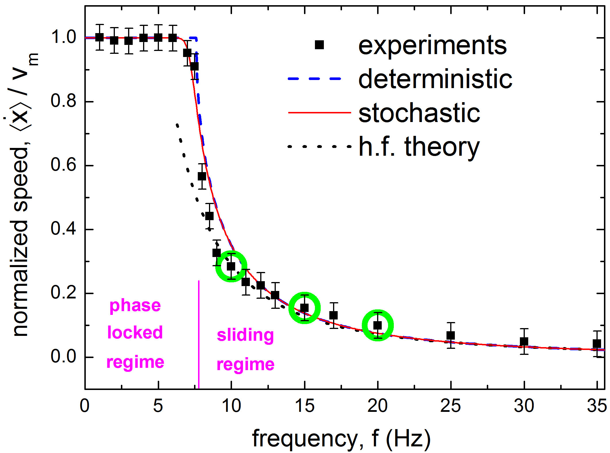
Fig.  2: Mean speed $\langle\dot{x}\rangle$ of a single particle normalized by $v_{\rm m}=\lambda f$ as a function of frequency $f$ for the case of circular polarization, $\beta=0$. The deterministic (dashed line) and stochastic (solid line) theoretical predictions, as in Eqs. (5) and (6), respectively, are fitted against the experimental data (filled squares). The dotted line corresponds to the high frequency (h. f.) theory, Eq. 8 in the text. Green circles indicate the cuts at frequencies $f=10$, $15$ and $20\;{\rm Hz}$ further analyzed in Fig. 3.

A paramagnetic particle of radius $a$ and volume $V=(4/3)\pi a^{3}$, subjected to an external field ${\mathbf{H}}$ acquires a dipole moment ${\mathbf{m}}=V\chi{\mathbf{H}}$, with $\chi$ being the effective volume susceptibility of particle. The energy of interaction of the induced dipole with the magnetic field ${\mathbf{B}}$ is $U_{\rm s}=-{\mathbf{m}}\cdot{\mathbf{B}}$. Assuming low fields and using the linear relation ${\mathbf{B}}=\mu_{\rm s}{\mathbf{H}}$, where $\mu_{\rm s}$ the permeability of the solvent, the energy becomes $U_{\rm s}=-V\chi\mu_{\rm s}{\mathbf{H}}^{2}$.

The total field above the FGF is given by a superposition $\mathbf{H}=\mathbf{H}^{\rm sub}+\mathbf{H}^{\rm ext}$ of the stray field of the substrate, $\mathbf{H}^{\rm sub}$, and the external field, $\mathbf{H}^{\rm ext}$. The external field with elliptic polarization has the form:

$${\mathbf{H}}^{\rm ext}=(H_{0x}\cos(2\pi ft),0,-H_{0z}\sin(2\pi ft)),$$ (1)

where $f$ is the frequency. The amplitude of modulation $H_{0}$ and the ellipticity parameter $\beta\in[-1,1]$ are defined as: ⁴³

$$H_{0}=\sqrt{\frac{H_{0x}^{2}+H_{0z}^{2}}{2}},\quad\beta=\frac{H_{0x}^{2}-H_{0z}^{2}}{H_{0x}^{2}+H_{0z}^{2}}\,,$$ (2)

such that $\beta=0$ corresponds to the case of circular polarization. In all the experiments, we keep $H_{0}$ fixed, and change the driving frequency and the ellipticity of the applied field.

The general expression for $\mathbf{H}^{\rm sub}$ can be obtained using the conformal mapping technique.^{41, 42} At a moderate modulation, $H_{0}\ll M_{\rm s}$, and at a particle elevation $z\simeq\lambda$, as in our experimental conditions, the expression for the stray field becomes independent of the form of modulation and can be simplified to:⁴²

$$\mathbf{H}^{\rm sub}=\frac{4M_{\rm s}}{\pi}{\rm e}^{-2\pi z/\lambda}\left(\cos\frac{2\pi x}{\lambda},0,-\sin\frac{2\pi x}{\lambda}\right),$$ (3)

where $M_{\rm s}$ denotes the film saturation magnetization.

The overdamped dynamics of a single particle in the global field ${\mathbf{H}}$ above the FGF can be described as the motion in the potential $U_{\rm s}=-V\chi\mu_{\rm s}{\mathbf{H}}^{2}$ taken at a fixed elevation (see Eq. 16 in Appendix A), within the framework of the Langevin equation,

$$\zeta\dot{x}=-\frac{\partial U_{\rm s}(x,t)}{\partial x}+\sqrt{2k_{\rm B}T\zeta}\,\xi(t)\,,$$ (4)

where $\zeta$ is the viscous friction coefficient, $k_{\rm B}T$ is the thermal energy, and the stochastic force modeled via the Gaussian white noise with zero mean, $\left<\xi(t)\right>=0$, and the autocorrelation $\left<\xi(t)\xi(t^{\prime})\right>=\delta(t-t^{\prime})$. This model admits a simple interpretation, in particular we quantify transport by analyzing the averaged speed of the particle.

3.1 Transport in a circularly polarized field, $\beta=0$

In the case of circular polarization, $\beta=0$, the potential can be approximated as a traveling harmonic wave, ⁴² $U_{\rm s}(x,t)\propto\cos(2\pi(x/\lambda-v_{\rm m}t))$. This expression describes a spatially periodic landscape with the period $\lambda$ and minima at the positions $x_{\rm min}(t)=n\lambda+v_{\rm m}t$ ($n=0,1,2,\dots$), which continuously translate with time with a constant speed $v_{\rm m}=\lambda f$ along the $x$ axis. Further, we proceed to rescaled variables by measuring the length, time, magnetic field, and energy in the units of $\lambda$, $\zeta\lambda^{2}/U_{0}$, $M_{\rm s}$, $U_{0}$, respectively. We choose the energy unit to be the characteristic energy of the interaction of an induced dipole with the field generated by the FGF, $U_{0}=V\chi\mu_{\rm s}M_{\rm s}^{2}$.

In these units, the averaged speed of the particle can be calculated as: ⁴²

$$\frac{\left<\dot{x}\right>_{\beta=0}}{v_{\rm m}}=\left\{\begin{array}[]{ll}1,&{\rm if}\;\;\tilde{f}<\tilde{f}_{\rm c}(0)\,,\\ 1-\sqrt{1-\tilde{f}_{\rm c}^{2}(0)/\tilde{f}^{2}}\,,&{\rm if}\;\;\tilde{f}>\tilde{f}_{\rm c}(0)\,,\\ \end{array}\right.$$ (5)

without thermal fluctuations and,

$$\frac{\left<\dot{x}\right>_{\beta=0}}{v_{\rm m}}=1-\frac{\sinh(\pi D)}{\pi D\,|I_{iD}(D_{\rm c})|^{2}}\,$$ (6)

with thermal fluctuations. Here, we have introduced three parameters,

$$h_{0}=\frac{H_{0}}{M_{\rm s}},\quad\tilde{f}=\frac{f\zeta\lambda^{2}}{U_{0}},\quad\sigma=\frac{k_{\rm B}T}{U_{0}},$$ (7)

which are, in order, the dimensionless amplitude, frequency, and strength of thermal fluctuations. Then, $\tilde{f}_{\rm c}(0)=16h_{0}{\rm e}^{-2\pi z}$ is the critical frequency at $\beta=0$, $D=\tilde{f}/(2\pi\sigma)$, $D_{\rm c}=\tilde{f}_{\rm c}(0)/(2\pi\sigma)$, and $I_{i\nu}(x)$ is the modified Bessel function of the first kind of an imaginary order.

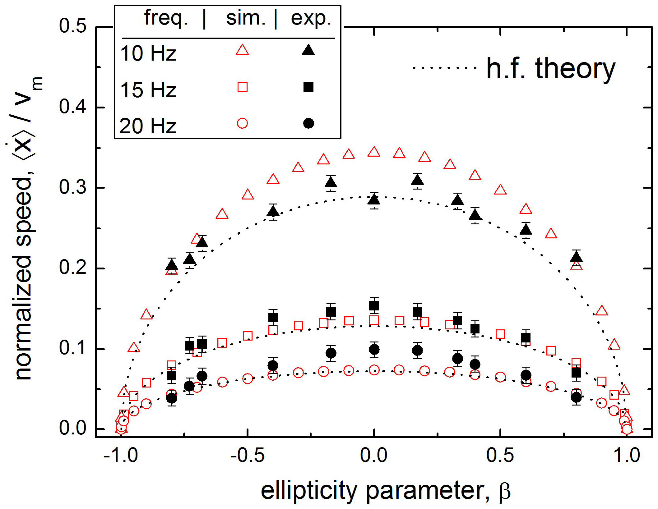
Fig.  3: The normalized mean speed, $\left<\dot{x}\right>/v_{\rm m}$, as a function of the ellipticity parameter, $\beta$, at three different frequencies, as shown by green circles in Fig. 2. The experimental data (filled markers) are plotted against the predictions of numerical simulations (open markers), Eq. 4, and of the h.f. theory (dotted lines), Eq. 8.

From Eqs. 5 and 6 it follows that, increasing the driving frequency, the system is characterized by two dynamic states separated by the critical value $\tilde{f}_{\rm c}$. This behaviour is also illustrated in Fig. 2, where we report measurements of the average speed of a single particle as a function of the driving frequency. The paramagnetic particle is driven above a garnet film by a circularly polarized ($\beta=0$) magnetic field with the amplitude $H_{0}=730\,{\rm A/m}$. At low frequencies, the particle is trapped in the minima of the translating potential, and moves with the maximal speed, $v_{\rm m}$. Beyond a critical frequency of $f_{\rm c}\approx 7.6\,{\rm Hz}$, the particle starts to lose its synchronization with the moving landscape entering into a “sliding” regime, where it decreases its average speed. Fig. 2 also shows that thermal fluctuations smooth the transition from the phase-locked dynamics to the sliding motion near the critical point. By fixing the particle elevation above the film to $z=0.923$ (in the units of $\lambda$), we estimated the dimensionless amplitude $h_{0}\approx 0.1457$ and noise strength of $\sigma\approx 2\times 10^{-5}$.

3.2 Transport in an elliptically polarized field, $\beta\neq 0$

The transition between the locked and sliding phases illustrated in Fig. 2 occurs also for different values of $\beta$, i.e. when the modulation has elliptic polarization. In particular, the critical frequency $\tilde{f}_{\rm c}$ depends on $\beta$, and we find that it shifts to lower frequencies, $\tilde{f}_{\rm c}(\beta)<\tilde{f}_{\rm c}(0)$. To gain insight into the sliding dynamics of a single particle at $\beta\neq 0$, we perform the time averaging of Eq. 4 taken in the deterministic limit, $\sigma=0$. The latter is justified by the fact that, as shown in Fig. 2, thermal fluctuations play a negligible role away from the critical frequency. As a result, the mean speed of a single particle is given by:

$$\frac{v_{0}(\beta)}{v_{\rm m}}=\frac{\left<\dot{x}\right>_{\rm hf}}{v_{\rm m}}=\frac{1}{2}\left(\frac{16h_{0}}{\tilde{f}}\right)^{2}{\rm e}^{-4\pi z}\sqrt{1-\beta^{2}}\quad(\tilde{f}\gg\tilde{f}_{c})\,$$ (8)

valid for any $\beta$ at high frequencies. A complete derivation of Eq. 8 is given in Appendix A. The accuracy of this prediction can be estimated from Fig. 2. Although the h. f. analysis is formally valid in the high frequency limit, $\tilde{f}/\tilde{f}_{\rm c}\gg 1$, we see that it works well already at $\tilde{f}/\tilde{f}_{\rm c}(0)\approx 2$ ($15\;{\rm Hz}$) and is still reasonable even at the lower frequency of $10\;{\rm Hz}$.

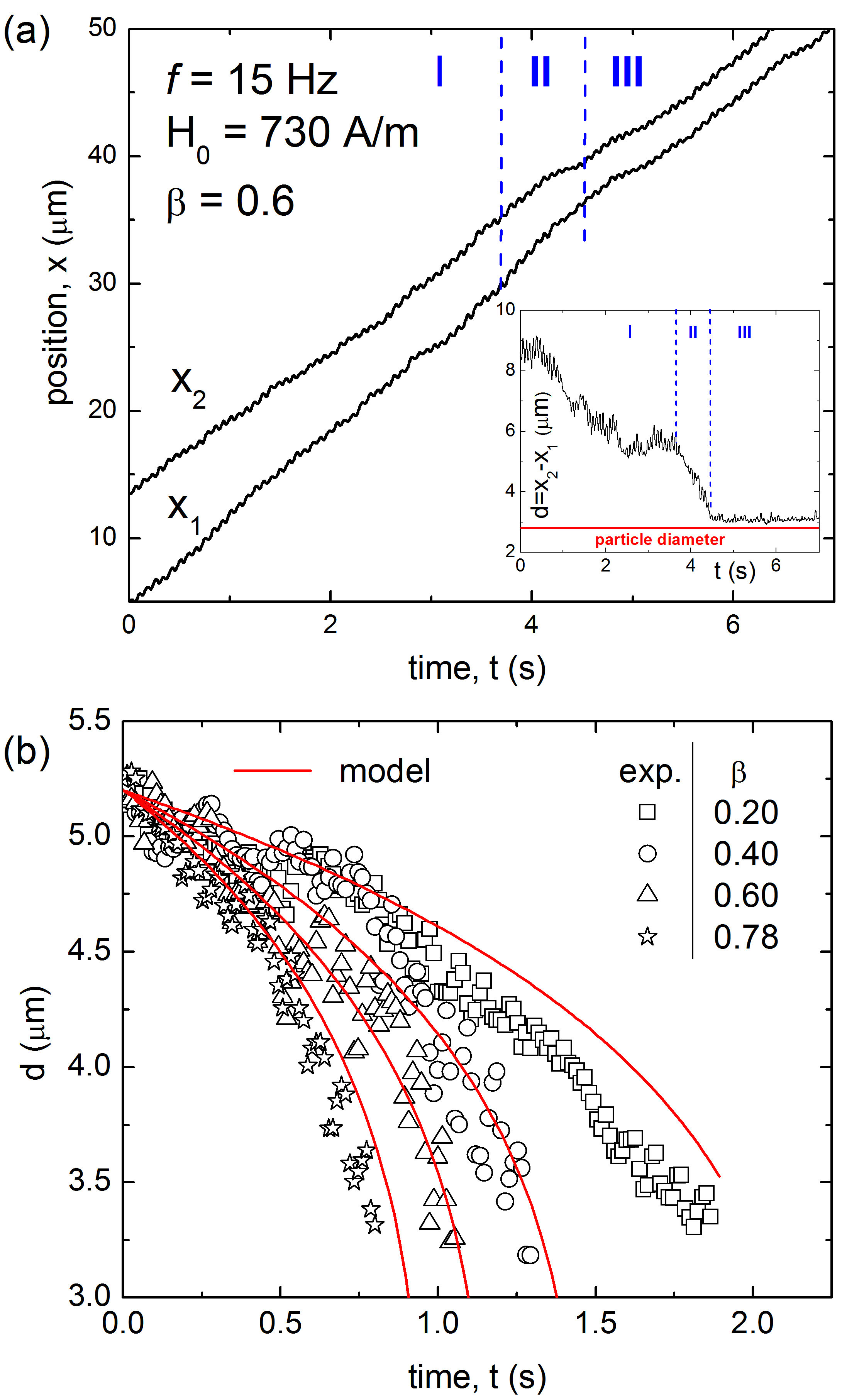
Fig.  4: (a) Positions $x_{1}$ and $x_{2}$ versus time $t$ of two approaching paramagnetic colloidal particles subjected to an external field with the frequency $f=15\,{\rm Hz}$, amplitude $H_{0}=730\,{\rm A/m}$, and ellipticity $\beta=0.6$. We distinguish three regimes: one characterized by a slow approach of the particles (I), a second characterized by dipolar attraction and leading to the doublet formation (II), and finally the last where particle motion occur in form of a doublet (III). Inset shows the separation distance $d=|x_{2}-x_{1}|$ versus time, $t$. (b) Separation distance $d$ versus time $t$ in regime II plotted at different $\beta$. Scattered points are experimental data, solid red lines are fits following the theoretical model, see Eq. 12 in the text.

In Fig. 3 we show the impact of the ellipticity of the field, $\beta$, on the average speed $\langle\dot{x}\rangle$ of a single particle and at three different driving frequencies. For circularly polarized field ($\beta=0$), $\langle\dot{x}\rangle$ is maximum for all frequencies, and it decreases as $\beta\neq 0$, in a symmetric way with respect to the positive and negative values of $\beta$ according to the root law $\left<\dot{x}\right>/v_{\rm m}\propto\sqrt{1-\beta^{2}}$. The experimental results are in good agreement with the predictions from Brownian dynamics simulation using Eq. 4 and the h. f. theory, Eq. 8, as described in Appendix A. Fig. 3 also shows that the h. f. approximation well represent the dependence of $\left<\dot{x}\right>$ on $\beta$.

4 Interacting particles

Increasing the number of particles, forces the latter to interact via magnetic dipolar interactions, see Appendix B for details. Experimentally, we observed a different behaviour depending whatever the particles were moving in the phase locked or in the sliding regime. In the first regime, the particles formed a series of chains equally spaced along the direction of motion ($x$), and all of them were moving at same average speed, $v_{\rm m}$. In this situation, even for large ellipticity, the particles always keep the difference in their $x$ coordinates constant, and it was not possible to induce attraction or repulsion, breaking the robust dynamic pattern. In contrast, in the sliding regime, each particle was unable to follow the fast dynamics of the translating potential and it lost the phase-locking with the field at different times. Since this process did not occur synchronously for all the particles, the moving colloids showed a certain degree of randomization in their speeds. As a consequence, between each pair of particles the average distance along $x$ was not always fixed, but it could increase or decrease depending on the relative speed. Thus, in the sliding regime, we found that it was possible to tune the particle interaction by changing $\beta$.

4.1 Two particles moving one behind another

To study the effects caused by the dipole-dipole interactions, we first analyze the one-dimensional situation in which a pair of particles has no relative displacement along the stripes ($y_{1}=y_{2}$), moving one behind the other in the sliding regime.

Fig. 4 shows the time evolution of the positions $x_{1}$ and $x_{2}$ of a pair of colloidal particles initially placed at a relative distance of $d=8.2\,{\rm\mu m}$, and driven above an FGF by an elliptically polarized magnetic field with amplitude $H_{0}=730\,{\rm A/m}$, frequency $f=15\,{\rm Hz}$ and ellipticity $\beta=0.6$. As we show below in this section, this value of $\beta$ corresponds to attracting dipolar interactions. The displacements shown in Fig. 4, illustrate the three regimes of motion. In the first one (regime I), the separation distance is too large to cause an evident effect of attraction, and the particles slowly approach each other due to a small difference in their speeds in the sliding regime. The relative dynamics is governed by the interplay between thermal fluctuations and the driving potential. Note that the separation distance $d=d(t)$ displays pronounced oscillations. As explicitly shown in Appendix A, these oscillations are caused by the external modulation and occur with the external frequency $f$. When the particles come close enough, to about $d\simeq 5.2\,{\rm\mu m}$ in our case, their relative motion speeds up and their distance $d$ rapidly decreases to a minimal distance dictated by steric interactions (regime II). After that the particles have formed a stable doublet (regime III) and propel as a whole. Note, however, that $d(t)$ does not remain equal to exactly the hard-core distance of $2a$.

To address the one-dimensional problem theoretically, we will apply the h.f. theory developed in Appendix C. The interaction of the

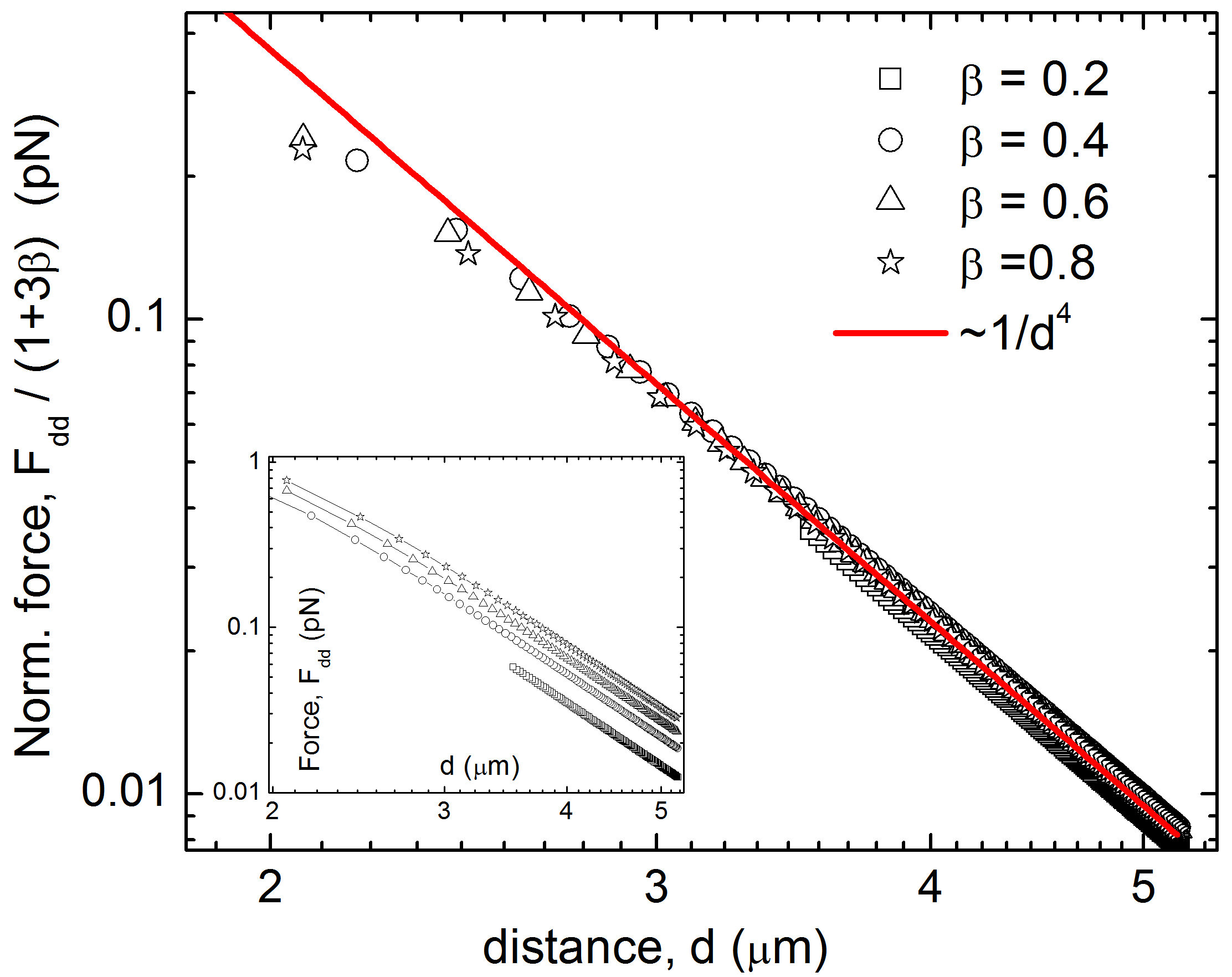
Fig.  5: Log-log plot of the force $F_{\rm dd}$ between a pair of particles normalized by $(1+3\beta)$ and plotted as a function of the separation distance $d$. Scattered data correspond to the lines fitting the experimental points in Fig. 4(b), solid red line is a fit according to Eq. 11, showing the dipolar nature of the interaction. Inset shows the force versus distance without the normalization for different values of $\beta$.

two particles with the slowly evolving coordinates ${\mathbf{R}}_{1}=(X_{1},Y_{1})$ and ${\mathbf{R}}_{2}=(X_{2},Y_{2})$ is described by the effective potential given by Eq. 33 or Eq. 34. Taking into account that $Y_{1}=Y_{2}$ (or $\vartheta=0$, where $\vartheta$ is the angle between the axis $x$ and the straight line going through the centers of particles) and introducing the distance between the particles as $d:=|X_{12}|=|X_{1}-X_{2}|$, we have $R=d$, $X_{12}^{2}/R^{2}=1$. Hence, the effective interaction potential that describes the slow dynamics of particles simplifies to

$$U_{\rm dd}(d)=-\frac{\alpha h_{0}^{2}(1+3\beta)}{2d^{3}}\,.$$ (9)

Whether the particles attract or repel depends on the sign of the factor $1+3\beta$. Setting it to zero, we find that the critical value is

$$\beta_{\rm c}(\vartheta=0)=-\frac{1}{3}\,.$$ (10)

For $\beta<\beta_{\rm c}$ the particles repel each other, while for $\beta>\beta_{\rm c}$ attraction takes place.

The separation distance satisfies the dimensionless equation $\dot{d}=-2\partial_{d}U_{\rm dd}=-3\alpha h_{0}^{2}(1+3\beta)/d^{4}$. Rewriting this equation back in the original variables, as before re-scaling, we obtain

$$\zeta\dot{d}=-\frac{k(1+3\beta)}{d^{4}}=:F_{\rm dd}(d)\,,$$ (11)

where the constant $k=3\mu_{s}(\chi VH_{0})^{2}/(4\pi)$. Thus, at a given field amplitude, $H_{0}$, the strength of interactions between a pair of particles scales with the ellipticity of the field, $\beta$, the susceptibility $\chi$ and size $a$ of particles as $F_{\rm dd}\propto(1+3\beta)\chi^{2}a^{6}$.

Assuming that at time $t=0$ the particles are initially separated by a distance $d=d_{0}$, we integrate Eq. 11 to find a power law for the separation distance as a function of time:

$$d(t)=\left(d_{0}^{5}-\frac{5k(1+3\beta)}{\zeta}t\right)^{1/5}\,,$$ (12)

From Eq. 12 follows that for $\beta<\beta_{c}(0)=-1/3$ ($\beta>\beta_{\rm c}(0)$), the separation distance increases (decreases) with time. During attraction, the particles approach till reaching a minimal distance $d_{\rm m}$ which for hard spheres is given by, $d_{\rm m}=2a$. From Eq. 12 it is possible also to estimate the time takes the particles to come into contact, as $\tau_{\rm c}=\zeta(d_{0}^{5}-d_{\rm m}^{5})/[5k(1+3\beta)]$.

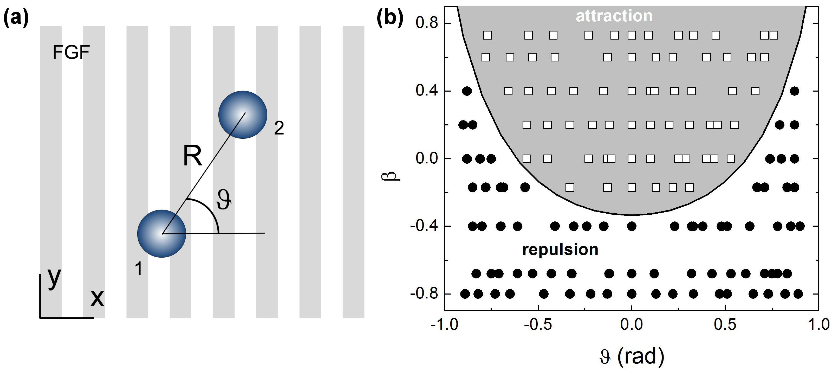
Fig.  6: (a) Schematic showing a pair of interacting particles driven above the FGF and having arbitrary positions in the plane $(x,y)$. (b) Phase diagram in the plane $(\vartheta,\beta)$, showing the regions of attraction and repulsion. Here, $\vartheta$ denotes the polar angle introduced as shown in panel (a). Scattered data are experimental points, solid line is according to Eq. 15.

In order to directly derive the strength of the dipolar interactions from the experimental data, we estimated the dependence of the force $F_{\rm dd}$ on the separation distance $d$. The inset of Fig. 5 shows the dependencies $F_{\rm dd}(d)$ for different $\beta$. The values of the force were computed using the Stokes law, $F_{\rm dd}=\zeta v_{\rm d}$, where the speeds $v_{\rm d}$ were recovered from the solid red curves in Fig. 4(b) that fit the experimental data. The friction coefficient was drawn from the relation $\zeta=6\pi\eta a$, where $\eta=10^{-3}\,{\rm Pa\cdot s}$ is the dynamic viscosity of water. Following Eq. 11, we expect the ratio $F_{\rm dd}/(1+3\beta)=k/d^{4}$ to be independent of the field ellipticity, $\beta$. This prediction is validated in Fig. 5, by plotting the force $F_{\rm dd}$ normalized by $1+3\beta$ as a function of the distance $d$. We note that all the dependencies for the different values of $\beta$ showed in the inset, collapse into the same curve. Furthermore, from the regression we obtain a value of the constant $k\approx 5.91\,{\rm pN\;\mu m^{4}}$, which is in good agreement with the theoretical prediction $k=3\mu_{s}(\chi VH_{0})^{2}/(4\pi)\approx 5.93\,{\rm pN\;\mu m^{4}}$, evaluated based on the experimental parameters, taking into account the uncertainty related to the exact value of $\chi$.³⁶ The magnetic permeability of the solvent was estimated as the permeability of free space.

We note that Eqs. 11 and 12 present purely deterministic predictions for the dipolar force and the separation distance. Similarly to the situation of a single particle, as e.g., in Fig. 2, thermal fluctuations are expected to slightly slow down the deterministic dynamics in regime II, as in Eq. 12. As confirmed by Brownian dynamics simulations, results not shown here, the thermal noise indeed effectively weakens the attractive forces shortly before the particles come into contact, thus slightly increasing the time of approach of the particles in regime II. This tendency can be also seen from Fig. 5, where the experimental data start to undershoot the deterministic predictions at small $d$, close to the smallest particle distance.

4.2 Particles with arbitrary positions

We now consider the general situation in which a pair of particles have arbitrary positions in the $(x,y)$ plane, and using the h. f. theory. First, we mention the motion of the center of mass of the two particles. The equation of motion for the center of mass, ${\mathbf{Q}}=({\mathbf{R}}_{1}+{\mathbf{R}}_{2})/2$, can be deduced from Eq. 32 in Appendix C. The center of mass moves strictly across the stripes with the constant speed of a single particle, and there is no displacement along the stripes, $\dot{\mathbf{Q}}=(\dot{Q},0)=v_{0}\hat{\mathbf{e}}_{x}$, irrespective of the positions of the particles in the plane $(x,y)$.

Then, we analyze the relative motion of particles. Instead of the Cartesian coordinates ${\mathbf{R}}_{12}=(X_{1}-X_{2},Y_{1}-Y_{2})$, it is convenient to proceed to the polar coordinates $(R,\vartheta)$ introduced such that ${\mathbf{R}}_{12}=R(\cos\vartheta,\sin\vartheta)$, where $R=\sqrt{(X_{1}-X_{2})^{2}+(Y_{1}-Y_{2})^{2}}$ is the distance between the particles, see Fig. 6(a). After the transformation, the equations of motion $\dot{R}=-2\partial_{R}U_{\rm dd}(R,\vartheta)$ and $R^{2}\dot{\vartheta}=-2\partial_{\vartheta}U_{\rm dd}(R,\vartheta)$ with $U_{\rm dd}(R,\vartheta)$ given by Eq. 34, result in:

$$\dot{R} = \frac{3\alpha h_{0}^{2}}{R^{4}}\left[2-3(1+\beta)\cos^{2}\vartheta\right],$$ (13)

$$\dot{\vartheta} = -\frac{3\alpha h_{0}^{2}(1+\beta)}{R^{5}}\sin 2\vartheta\,.$$ (14)

By setting $\dot{R}=0$ in Eq. 13 we consider the marginal case that separates the situations of repulsion, $\dot{R}>0$, and attraction, $\dot{R}<0$. This condition gives us the critical value of the ellipticity parameter,

$$\beta_{\rm c}(\vartheta)=-1+\frac{2}{3\cos^{2}\vartheta}\,,$$ (15)

generalized for arbitrary values of $\vartheta$. Again, the condition $\beta<\beta_{\rm c}$ corresponds to repulsion, while the opposite case $\beta>\beta_{\rm c}$ is responsible for attraction. In the partial case of the particles moving along the $x$ direction, $\vartheta=0$, Eq. 15 predicts $\beta_{\rm c}(0)=-1/3$, in agreement with the earlier considered case, see Eq. 10. The opposite partial case of particles traveling across the stripes side by side, $\vartheta=\pi/2$, is always repulsive, which is seen from Eq. 13, since $\dot{R}>0$. A repulsion-attraction diagram, which demonstrates agreement between the theory and experiment, is shown in Fig. 6(b).

We note that this analysis implies that the angle $\vartheta$ is constant and refers not only to a given position but also to a given instant of time. However, the polar angle $\vartheta$ generally evolves in time. As follows from Eq. 14, it admits two fixed points, $\vartheta_{0}^{(1)}=0,\pi$ and $\vartheta_{0}^{(2)}=\pm\pi/2$. The first one, when the particles move one behind another across the stripes, is stable. The second one, when the particles travel across the stripes side by side and attract or repel along the stripes, is unstable. The evolution of the angle is determined by the sign of $\sin 2\vartheta$ and we conclude that independent of the ellipticity $\beta$, the particles evolve towards the stable state with $\vartheta=0,\pi$. In other words, the particles tend to reorient such that the straight line through the centers of particles aligns along the $x$ axis.

5 Conclusions

In this article, we studied both experimentally and theoretically the dynamics of interacting paramagnetic colloidal particle magnetically driven above a stripe patterned garnet film. We show that attractive dipolar interactions between propagating particles become important for distances lower than $d_{0}\sim 6{\rm\mu m}$ for the used field strength of $H_{0}=730\,{\rm A/m}$, although this distance can be tuned by changing the amplitude of the applied field $H_{0}$. When particles approach closer than $d_{0}$, they form stable doublets which move at a constant mean speed along the modulated landscape.

The suggested theoretical model, which describes the slow dynamics of interacting particles averaged over the fast oscillatory time scale, is analytically tractable. It captures the experimental results quantitatively well. In particular, we gain an insight into the details underlying the interaction, by outlining an effective interaction potential. These findings can be used to extend the model towards more complicated situations, involving a large number of particles or binary mixtures driven above a garnet film. On the other hand, the application of a similar approach is potentially promising for studying the transport of interacting particles in other systems using magnetic structure substrates. ^{44, 45, 46, 47, 48}

The possibility to tune the sign of the inter-particle interactions and their relative strength in transport at small scales has potential applications in microfluidics and lab-on-a-chip systems. In particular, it can be used to pick up and capture a microscopic cargo between attractive particles, transport and finally release it at a prescribed location by switching the attractive interaction to become repulsive.

Furthermore, the use of attractive interactions between the moving particles can be used to generate longer chains traveling along the modulated landscapes, as shown for smaller particles. ³⁴ These chains can serve as a model to study fluctuations in driven Brownian worms,⁴⁹ or novel ratchet effects arising from condensed particle trains.^{50, 51, 52}

Appendix

Appendix A Slow dynamics of a single particle

At high frequencies, different times scales naturally present in the system become well separated and admit the possibility to reduce the complexity by effectively decoupling the fast and slow motions. ⁵³ The “fast” dynamics is associated with the external driving with the characteristic time scale $\tau_{\rm f}=1/f$. The “slow” motion, such as, propulsion of a single particle across the stripes in our system, is the “net” or mean (time-averaged) response of the system at time scales $t\gg\tau_{\rm f}$.

We now consider the overdamped motion of a single particle in the field ${\mathbf{H}}$ above the substrate, which is described by the dimensionless potential

$$U_{\rm s}(x,t)=-\frac{8h_{0}}{\pi}{\rm e}^{-2\pi z}\left[u_{1}\cos(2\pi x)+u_{2}\sin(2\pi x)\right]$$ (16)

with $u_{1}(\beta,t)=\sqrt{1+\beta}\cos(2\pi\tilde{f}t)$ and $u_{2}(\beta,t)=\sqrt{1-\beta}\sin(2\pi\tilde{f}t)$. To obtain the description for the slow motion of the particle, we have to perform a time averaging of Eq. 4 without thermal noise

$$\dot{x}(t) = -\partial_{x}U_{\rm s}(x,t)=F_{\rm s}(x,t)\,,$$ (17)

$$F_{\rm s}(x,t) = -16h_{0}{\rm e}^{-2\pi z}\left[u_{1}\sin(2\pi x)-u_{2}\cos(2\pi x)\right].\quad$$ (18)

The problem is considered deterministic, $\sigma=0$, because, as explained in the main text, thermal fluctuations are negligible for high-frequencies, $\tilde{f}\gg\tilde{f}_{\rm c}$. Following the method of averaging,^{54, 55, 56} we present the solution as a superposition:

$$x(t)=X(t)+\delta x(t),\quad\delta x(t)=\tilde{x}{\rm e}^{2\pi i\tilde{f}t}+\tilde{x}^{\ast}{\rm e}^{-2\pi i\tilde{f}t}\,,$$ (19)

where $X(t)$ and $\delta x(t)$ describe the slow (time-averaged over the period $1/\tilde{f}$ of modulation) coordinate and its fast (time-periodic) counterpart oscillating with the frequency $\tilde{f}$, respectively. The quickly evolving contribution $\delta x(t)$, which has to be considered small compared to $X(t)$, is then represented via the complex amplitude $\tilde{x}$ and its complex conjugated pair $\tilde{x}^{\ast}$, as in Eq. 19. The complex amplitudes do not explicitly depend on the fast time $\tilde{f}t$. We note that it is convenient to use exponential representation of the functions $\cos(2\pi\tilde{f}t)$ and $\sin(2\pi\tilde{f}t)$. The spatially dependent functions $\cos(2\pi x)$ and $\sin(2\pi x)$ are expanded using the smallness of $\delta x$, according to $g(x)=g(X+\delta x)\approx g(X)+\partial_{x}g(X)\delta x$.

Substituting the ansatz 19 into Eq. 17, using the described representations, and retaining the leading terms, we find for the complex amplitude:

$$\tilde{x}(X)=\frac{4h_{0}}{\pi\tilde{f}}{\rm e}^{-2\pi z}\left[i\sqrt{1+\beta}\sin(2\pi X)-\sqrt{1-\beta}\cos(2\pi X)\right].$$ (20)

To obtain the equation for $X$, we perform the time-averaging of Eq. 17. We evaluate the time-averaged contributions, $\overline{\sin(2\pi x)\cos(2\pi\tilde{f}t)}=\pi(\tilde{x}^{\ast}+\tilde{x})\cos(2\pi X)=-(8h_{0}/\tilde{f}){\rm e}^{-2\pi z}\sqrt{1-\beta}\cos^{2}(2\pi X)$ and $\overline{\cos(2\pi x)\sin(2\pi\tilde{f}t)}=i\pi(\tilde{x}^{\ast}-\tilde{x})\sin(2\pi X)=-(8h_{0}/\tilde{f}){\rm e}^{-2\pi z}\sqrt{1+\beta}\sin^{2}(2\pi X)$. Here, the overlines denote the time averaging over the period of modulation, $\overline{\mathcal{F}}=\tilde{f}\int_{0}^{1/\tilde{f}}\mathcal{F}\,dt$, and the combinations $\tilde{x}^{\ast}+\tilde{x}=2\,{\rm Re}(\tilde{x})$ and $i(\tilde{x}^{\ast}-\tilde{x})=2\,{\rm Im}(\tilde{x})$ are evaluated via the real and imaginary parts of Eq. 20. As a result, the time averaged equation takes a simple form

$$v_{0}(\beta):=\dot{X}=\left<\dot{x}\right>_{\rm hf}=\frac{1}{2}\frac{(16h_{0})^{2}}{\tilde{f}}{\rm e}^{-4\pi z}\sqrt{1-\beta^{2}}\,,$$ (21)

which, being written relative to the maximal speed, $v_{\rm m}=\tilde{f}$, gives Eq. 8.

Because the equation for the slow dynamics of a single particle is independent of $X$ and $t$, it means that the particle moves on the average with a constant speed. Therefore, expression 21 is interpreted as the mean speed in the sliding regime, valid at high frequencies and at all $\beta$. As follows from Eq. 21, the time averaged motion of a single particle is equivalent to the motion in the mean potential

$$U_{\rm s}(X)=-v_{0}X\,.$$ (22)

It should be noted that time averaging directly the potential in favor of the equations of motion, can lead to misleading results. For instance, performing the averaging of Eq. 16 does not lead to Eq. 22 but results in identically vanishing $U_{\rm s}(X)$, which incorrectly predicts no motion.

Appendix B Magnetic dipolar interactions

In a suspension of magnetic dipoles, each dipole interacts with the fields produced by all other dipoles. Induced dipole $l$ with the magnetic moment ${\mathbf{m}}_{l}=V\chi{\mathbf{H}}_{l}$ interacts with the field ${\mathbf{B}}_{l^{\prime}}=\mu_{s}{\mathbf{H}}_{l^{\prime}}$ generated by particle $l^{\prime}$, leading to the dipolar energy $U_{\rm dd}=-{\mathbf{m}}_{l}\cdot{\mathbf{B}}_{l^{\prime}}=-{\mathbf{m}}_{l^{\prime}}\cdot{\mathbf{B}}_{l}$. Thus, for a system of dipoles with the coordinates ${\mathbf{r}}_{l}$ the total energy can be written as:

$$U=\sum_{l}U_{\rm s}({\mathbf{r}}_{l},t)+\frac{1}{2}\sum_{l}\sum_{l^{\prime}\neq l}U_{\rm dd}({\mathbf{r}}_{ll^{\prime}},t)\,.$$ (23)

Here, the first contribution stands for the interaction of each single dipole with the nonuniform magnetic field above the FGF and the second term describes the dipolar interactions with the pairwise potential

$$U_{\rm dd}({\mathbf{r}}_{ll^{\prime}},t)=-\frac{\mu_{s}V^{2}\chi^{2}}{4\pi}\left[3\,\frac{{\mathbf{H}}_{l}\cdot{\mathbf{r}}_{ll^{\prime}}\,{\mathbf{H}}_{l^{\prime}}\cdot{\mathbf{r}}_{ll^{\prime}}}{r_{ll^{\prime}}^{5}}-\frac{{\mathbf{H}}_{l}\cdot{\mathbf{H}}_{l^{\prime}}}{r_{ll^{\prime}}^{3}}\right],$$ (24)

where ${\mathbf{H}}_{l}={\mathbf{H}}({\mathbf{r}}_{l},t)$, ${\mathbf{r}}_{ll^{\prime}}={\mathbf{r}}_{l}-{\mathbf{r}}_{l^{\prime}}$, and $r_{ll^{\prime}}=|{\mathbf{r}}_{ll^{\prime}}|$. By measuring the lengths in the scale of $\lambda$ and energy in the units of $U_{0}=V\chi\mu_{s}M_{\rm s}^{2}$ as before and accounting for Eq. 24, the dimensionless expression for the total energy, Eq. 23, becomes

$$U=-\sum_{l}{\mathbf{H}}^{2}_{l}-\frac{1}{2}\alpha\sum_{l}\sum_{l^{\prime}\neq l}\left[3\,\frac{{\mathbf{H}}_{l}\cdot{\mathbf{r}}_{ll^{\prime}}\,{\mathbf{H}}_{l^{\prime}}\cdot{\mathbf{r}}_{ll^{\prime}}}{r_{ll^{\prime}}^{5}}-\frac{{\mathbf{H}}_{l}\cdot{\mathbf{H}}_{l^{\prime}}}{r_{ll^{\prime}}^{3}}\right].$$ (25)

The dimensionless parameter

$$\alpha=\frac{\chi}{4\pi}\frac{V}{\lambda^{3}}=\frac{\chi}{3}\left(\frac{a}{\lambda}\right)^{3}\,$$ (26)

determines the strength of dipole-dipole interactions relative to the energy of interaction with the FGF, $U_{0}$. For our experimental system, $\alpha\approx 0.027$, if $\chi=0.53$.

Appendix C Slow dynamics of two interacting particles

The interaction potential between the driven particles taking into account the dipolar interactions is quite complicated, since it consists of different contributions resulting from the temporal modulation, the field of substrate and their interplay, described by terms of order $\mathcal{O}(h_{0}^{2})$, $\mathcal{O}(h_{0}{\rm e}^{-2\pi z})$, and $\mathcal{O}({\rm e}^{-4\pi z})$, respectively. At our experimental conditions ($h_{0}\ll 1$, $z\simeq 1$), the mean drift of particles is due to the interplay of temporal modulation and the field of substrate. In contrast to the latter, the leading contribution to the dipole-dipole interaction potential is to a high accuracy governed by the terms of order $\mathcal{O}(h_{0}^{2})$, as caused purely by the temporal modulation.

Evaluating the leading part of the dipole-dipole interaction potential for a pair of particles with the coordinates ${\mathbf{r}}_{l}=(x_{l},y_{l})$ and $l,l^{\prime}\in\{1,2\}$, $l^{\prime}\neq l$ (the elevation $z$ is fixed), yields:

$$U_{\rm dd}({\mathbf{r}}_{12})=\alpha h_{0}^{2}\left[\frac{s_{1}}{r^{3}}-\frac{s_{2}({\mathbf{r}}_{12}\cdot\hat{\mathbf{e}}_{x})^{2}}{r^{5}}\right]\,$$ (27)

with the time-dependent functions $s_{1}(\beta,t)=1+\beta\cos(4\pi\tilde{f}t)$ and $s_{2}(\beta,t)=(3/2)(1+\beta)(1+\cos(4\pi\tilde{f}t))$. Here, $\hat{\mathbf{e}}_{x}=(1,0,0)$ is the unit vector along the $x$ axis, ${\mathbf{r}}_{12}={\mathbf{r}}_{1}-{\mathbf{r}}_{2}$, and $r=|{\mathbf{r}}_{12}|$ is the distance between the particles.

The deterministic dynamics of the pair of particles, including the motion in the FGF potential, Eq. 16, and the dipole-dipole interactions as in Eq. 27, obeys the equations:

$$\dot{\mathbf{r}}_{l}=F_{\rm s}\hat{\mathbf{e}}_{x}+\frac{\alpha h_{0}^{2}}{r^{5}}\left[\left(3s_{1}-5s_{2}\frac{x_{ll^{\prime}}^{2}}{r^{2}}\right){\mathbf{r}}_{ll^{\prime}}+2s_{2}x_{ll^{\prime}}\hat{\mathbf{e}}_{x}\right],$$ (28)

where $F_{\rm s}(x_{l},t)$ is the force exerted on dipole $l$ by the field of substrate, see Eq. 18. In the case of no dipole-dipole interaction, $\alpha=0$, the dynamics of particles reduces to the independent but identical one-dimensional translation across the stripes, as described by Eqs. 17 and 18, which admit no relative motion. The relative motion comes into play when the particles start to interact, $\alpha>0$.

To describe the slow dynamics of interacting particles, we perform the time-averaging of Eqn. 28. We note that in addition to fast evolving functions in $F_{\rm s}$ oscillating with frequency $\tilde{f}$, the dipole-dipole interactions also excite oscillations with the double frequency, $2\tilde{f}$, entering via the functions $s_{1}$ and $s_{2}$. This time dependence suggests the corresponding ansatz:

$${\mathbf{r}}_{l}(t)={\mathbf{R}}_{l}(t)+\mathbf{\delta r}_{l}(t),\quad\mathbf{\delta r}_{l}=\mathbf{\delta r}_{l}^{(1)}+\mathbf{\delta r}_{l}^{(2)}\,,$$ (29)

$$\mathbf{\delta r}_{l}^{(1)}=\tilde{\mathbf{r}}_{l}^{(1)}{\rm e}^{2\pi i\tilde{f}t}+\textrm{c.c.},\quad\mathbf{\delta r}_{l}^{(2)}=\tilde{\mathbf{r}}_{l}^{(2)}{\rm e}^{4\pi i\tilde{f}t}+\textrm{c.c.}\,,$$ (30)

where ${\mathbf{R}}_{l}=(X_{l},Y_{l})=\tilde{f}\int_{0}^{1/\tilde{f}}{\mathbf{r}}_{l}(t)\,dt$ denotes the solution averaged over the fast oscillatory timescales, the superscripts “$(1)$” and “$(2)$” are used to mark the solutions oscillating with the single ($\tilde{f}$) and double ($2\tilde{f}$) frequency, respectively. The $\tilde{\mathbf{r}}_{l}^{(j)}$ stand for the complex amplitudes and c.c. means the complex conjugate. Note that the leading part of solution for ${\mathbf{r}}_{l}^{(1)}=(\tilde{x}(X_{l}),0)$ is determined by the earlier considered case $\alpha=0$ with $\tilde{x}(X_{l})$ given by $\tilde{x}(X_{l})$ in Eq. 20.

Before we proceed to the derivation of the complex amplitudes ${\mathbf{r}}_{l}^{(2)}$, we expand all spatially dependent functions in Eqn. 28 as $g({\mathbf{r}}_{12})\approx g({\mathbf{R}}_{12})+\partial_{{\mathbf{r}}_{12}}g({\mathbf{R}}_{12})\cdot\mathbf{\delta r}_{12}$. Retaining the leading contributions, for the evolution of the solution evolving with the double frequency we obtain the equations: $\partial_{t}\boldsymbol{\delta}{\mathbf{r}}_{l}^{(2)}=\alpha h_{0}^{2}/R^{5}[(3\tilde{s}_{1}-5\tilde{s}_{2}X_{ll^{\prime}}^{2}/R^{2})\mathbf{R}_{ll^{\prime}}+2\tilde{s}_{2}X_{ll^{\prime}}\hat{\mathbf{e}}_{x}]$. Here, $\tilde{s}_{1}=\beta\cos(4\pi\tilde{f}t)$ and $\tilde{s}_{2}=(3/2)(1+\beta)\cos(4\pi\tilde{f}t)$ are the quickly evolving parts of functions $s_{1}$ and $s_{2}$ oscillating with the double frequency, $2\tilde{f}$. Using the exponential representation of the function $\cos(4\pi\tilde{f}t)$ and taking into account the explicit temporal dependence in $\mathbf{\delta r}^{(2)}$, see Eq. 30, we solve the above equations for the complex amplitudes to arrive at:

$$\tilde{\mathbf{r}}_{l}^{(2)}=-\frac{3i\alpha h_{0}^{2}}{16\pi\tilde{f}R^{5}}\left[{\mathbf{p}}(\beta,{\mathbf{R}}_{ll^{\prime}})-5(1+\beta)\frac{X_{ll^{\prime}}^{2}}{R^{2}}{\mathbf{R}}_{ll^{\prime}}\right],$$ (31)

with ${\mathbf{p}}=(2(1+2\beta)X_{ll^{\prime}},2\beta Y_{ll^{\prime}})$. From Eq. 31 for $\tilde{y}_{l}^{(2)}$ we see that oscillations along the stripes of the FGF occur only if the particles have different $y$ coordinates, $Y_{12}\neq 0$. For a pair of particles moving across the stripes one behind another no oscillations transverse to the propagation direction takes place.

The relative contribution of the quickly oscillating solutions scales as: $|\tilde{\mathbf{r}}_{l}^{(2)}|/|\tilde{\mathbf{r}}_{l}^{(1)}|\simeq\alpha h_{0}{\rm e}^{2\pi z}/R^{4}$. For our system, the enumerator can be of order $1$. This means that when particles are widely separated, $R\gg 1$, the fast dynamics corresponds to oscillations (around the time-averaged solution) with the frequency $\tilde{f}$. As long as particles come closer, the relative amplitude of oscillations with the double frequency increases and at separations about few diameters, the fast dynamics presents the superposition of oscillations with both frequencies, $\tilde{f}$ and $2\tilde{f}$, around the slowly evolving state.

We are now ready to figure out the leading contributions into the time-averaged equations. Taking into account the solutions that determine the fast dynamics, we average over time Eqs. 28 and arrive at the equations:

$$\dot{\mathbf{R}}_{l}=v_{0}\hat{\mathbf{e}}_{x}+\frac{\alpha h_{0}^{2}}{R^{5}}\left[\left(3S_{1}-5S_{2}\frac{X_{ll^{\prime}}^{2}}{R^{2}}\right){\mathbf{R}}_{ll^{\prime}}+2S_{2}X_{ll^{\prime}}\hat{\mathbf{e}}_{x}\right],$$ (32)

where $v_{0}$ is given by Eq. 21 and $S_{1}=\overline{s}_{1}=1$, $S_{2}=\overline{s}_{2}=(3/2)(1+\beta)$ are the time averaged counterparts of the functions $s_{1}$ and $s_{2}$.

The time-averaged effect of dipole-dipole interaction of a pair of particles is described by the effective potential:

$$U_{\rm dd}({\mathbf{R}}_{12})=\frac{\alpha h_{0}^{2}}{R^{3}}\left[1-\frac{3(1+\beta)}{2}\frac{X_{12}^{2}}{R^{2}}\right],$$ (33)

where ${\mathbf{R}}_{12}={\mathbf{R}}_{1}-{\mathbf{R}}_{2}=(X_{1}-X_{2},Y_{1}-Y_{2})$ and $R=|{\mathbf{R}}_{12}|$. Alternatively, if we introduce the polar angle $\vartheta$ such that ${\mathbf{R}}_{12}=R(\cos\vartheta,\sin\vartheta)$, then:

$$U_{\rm dd}(R,\vartheta)=\frac{\alpha h_{0}^{2}}{R^{3}}\left[1-\frac{3}{2}(1+\beta)\cos^{2}\vartheta\right].$$ (34)

Finally, we note that the same effective potential, Eq. 33, would follow from Eq. 27, if we naively replaced functions $s_{1}$, $s_{2}$ and all the coordinates by their time-averaged counterparts. This result, however, is not obvious a priori, before the order of magnitude of the oscillating contributions is evaluated. We have also made a more careful analysis of other time averaged contributions such as e.g., the effects of the double frequency harmonics on the single particle motion and of the substrate field on the dipole-dipole interaction potential. The analysis shows that all these contributions present only small corrections to the leading one, as obtained in this section.

References

- 1 M. von Smoluchowski, Phys. Z., 1912, 13, 1069.
- 2 F. Jülicher, A. Ajdari and J. Prost, Rev. Mod. Phys., 1997, 69, 1269.
- 3 P. Reimann, Phys. Rep., 2002, 361, 57.
- 4 P. Hänggi and F. Marchesoni, Rev. Mod. Phys., 2009, 81, 387.
- 5 J. E. Villegas, S. Savel’ev, F. Nori, E. M. Gonzalez, J. V. Anguita, R. García, J. L. Vicent Science, 2003, 302, 1188.
- 6 J. B. Majer, J. Peguiron, M. Grifoni, M. Tusveld, and J. E. Mooij, Phys. Rev. Lett., 2003, 90, 056802.
- 7 H. Linke, T. E. Humphrey, A. Löfgren, A. O. Sushkov, R. Newbury, R. P. Taylor, P. Omling, Science, 1999, 286, 2314.
- 8 C. M.-Robilliard, D. Lucas, S. Guibal, J. Tabosa, C. Jurczak, J.-Y. Courtois, and G. Grynberg, Phys. Rev. Lett., 1999, 82, 851.
- 9 A. Engel, H. W. M ller, P. Reimann, and A. Jung, Phys. Rev. Lett., 2003, 91, 060602.
- 10 D. van der Meer, P. Reimann, K. van der Weele, and D. Lohse, Phys. Rev. Lett., 2004, 92, 184301.
- 11 N. J. Cordova, B. Ermentrout, and G. F. Oster, Proc. Natl. Acad. Sci. USA., 1992, 89, 339.
- 12 J. C. M. Gebhardt, A. E.-M. Clemen, J. Jaud, and M. Rief, Proc. Natl. Acad. Sci. USA., 2006, 103, 8680.
- 13 R. A. Cross, Proc. Natl. Acad. Sci. USA, 2006, 103, 8911.
- 14 C. Peskin, G. Odell, and G. Oster Biophys. J., 1993, 65, 316.
- 15 D. Pantaloni, C. L. Clainche, and M. F. Carlier Science, 2001, 292, 1502.
- 16 A. Mogilner, and G. Oste, Biophys. J., 2003, 84, 1591.
- 17 J. Rousselet, L. Salome, A. Ajdari, and J. Prost, Nature, 1994, 370, 446.
- 18 L. P. Faucheux, L. S. Bourdieu, P. D. Kaplan, and A. J. Libchaber Phys. Rev. Lett., 1995, 74, 1504.
- 19 C. Marquet, A. Buguin, L. Talini, and P. Silberzan, Phys. Rev. Lett., 2002, 88, 168301.
- 20 S.-H. Lee, K. Ladavac, M. Polin, and D. G. Grier, Phys. Rev. Lett., 2005, 94, 110601.
- 21 P. Tierno, S. V. Reddy, M. G. Roper, T. H. Johansen, and T. M. Fischer, J. Phys. Chem. B, 2008, 112, 3833.
- 22 J. C. Crocker and D. G. Grier, Phys. Rev. Lett., 1994, 73, 352.
- 23 G. M. Kepler and S. Fraden, Phys. Rev. Lett., 1994, 73, 356.
- 24 O. G. Calderón and S. Melle, J. Phys. D, 2002, 35, 2492.
- 25 S. L. Biswal and A. P. Gast, Phys. Rev. E, 2004, 69, 041406.
- 26 P. Tierno, R. Muruganathan, and T. M. Fischer, Phys. Rev. Lett., 98, 028301.
- 27 B. Yellen, O. Hovorka and G. Friedman, Proc. Natl. Acad. Sci. USA, 2005, 102, 8860.
- 28 P. Tierno, F. Sagus, T. H. Johansen, T. M. Fischer, Phys. Chem. Chem. Phys., 2009, 11, 9615.
- 29 A. H. Romero, A. M. Lacasta, and J. M. Sancho, Phys. Rev. E, 2004, 69, 051105.
- 30 E. Heinsalu, M. Patriarca, and F. Marchesoni, Phys. Rev. E, 2008, 77, 021129.
- 31 D. Speer, R. Eichhorn, M. Evstigneev, and P. Reimann, Phys. Rev. E, 2012, 85, 061132.
- 32 C. Reichhardt and C.J. Olson Reichhardt, Phys. Rev. E, 2005, 72 032401.
- 33 A. Libal, C. Reichhardt, B. Janko, and C.J. Olson Reichhardt Phys. Rev. Lett, 2006, 96 188301.
- 34 P. Tierno, Phys. Rev. Lett., 2012, 109, 198304.
- 35 S. Jaeger and S. H. L. Klapp, Phys. Rev. E, 2012, 86, 061402.
- 36 The exact value of is difficult to estimate since, in general, it depends on the magnetic doping of the paramagnetic colloids, which can vary from one stock solution to another.
- 37 L. E. Helseth, T. Backus, T. H. Johansen, and T. M. Fischer, Langmuir, 2005, 21, 7518.
- 38 P. Tierno, Soft Matter, 2012, 8, 11443.
- 39 W. F. Druyvesteyn, D. L. A. Tjaden and J. W. F. Dorleijn, Philips Res. Rep., 1972, 27, 7.
- 40 J. C. Crocker and D. G. Grier, J. Colloid Interface Sci., 1996, 179, 298.
- 41 P. Tierno, S. V. Reddy, T. H. Johansen, and T. M. Fischer, Phys. Rev. E 2007, 75, 041404.
- 42 A. V. Straube, and P. Tierno Europhys. Lett., 2013, 103, 28001.
- 43 S. Lacis, J. C. Bacri, A. Cebers, and R. Perzynski, Phys. Rev. E, 1997, 55, 2640.
- 44 B. B. Yellen, R. M. Erb, H. S. Son, R. Hewlin, H. Shang, G. U. Lee, Lab on a Chip, 2007, 7, 1681.
- 45 L. Gao, N. J. Gottron, L. N. Virgin, B. B. Yellen, Lab on a Chip, 2010, 10, 2108.
- 46 L. Gao, M. A. Tahir, L. N. Virgin, B. B. Yellen BB, Lab on a Chip, 2011, 11, 4214.
- 47 K. Gunnarsson, P. E. Roy, S. Felton, J. Pihl, P. Svedlindh, S. Berner, H. Lidbaum, S. Oscarsson, Adv. Mater., 2005, 17, 1730.
- 48 A. Ehresmann, D. Lengemann, T. Weis, A. Albrecht, J. Langfahl-Klabes, F. Göllner, D. Engel, Adv. Mater., 2011, 23, 5568.
- 49 R. Toussaint, G. Helgesen and E. G. Flekkoy, Phys. Rev. Lett., 2004, 93, 108304.
- 50 J. Dzubiella, G. P. Hoffmann, and H. Löwen, Phys. Rev. E, 2002, 65, 021402.
- 51 C. Reichhardt, C. J. Olson Reichhardt, Phys. Rev. E, 2006, 74, 011403.
- 52 A. Pototsky, A. J. Archer, M. Bestehorn, D. Merkt, S. Savelév, and F. Marchesoni, Phys. Rev. E, 2010, 82, 030401.
- 53 A. V. Straube, D. V. Lyubimov and S. V. Shklyaev, Phys. Fluids, 2006, 18, 053303.
- 54 A. H. Nayfeh, Introduction to Perturbation Techniques, Wiley, New York, 1981.
- 55 D. L. Piet, A. V. Straube, A. Snezhko and I. S. Aranson, Phys. Rev. Lett., 2013, 110, 198001.
- 56 D. L. Piet, A. V. Straube, A. Snezhko and I. S. Aranson, Phys. Rev. E, 2013, 88, 033024.