Phase Transitions in a System of Hard Rectangles on the Square Lattice
Abstract
The phase diagram of a system of monodispersed hard rectangles of size on a square lattice is numerically determined for and aspect ratio . We show the existence of a disordered phase, a nematic phase with orientational order, a columnar phase with orientational and partial translational order, and a solid-like phase with sublattice order, but no orientational order. The asymptotic behavior of the phase boundaries for large are determined using a combination of entropic arguments and a Bethe approximation. This allows us to generalize the phase diagram to larger and , showing that for , the system undergoes three entropy driven phase transitions with increasing density. The nature of the different phase transitions are established and the critical exponents for the continuous transitions are determined using finite size scaling.
pacs:
64.60.De, 64.60.Cn, 05.50.+qI Introduction
The study of entropy-driven phase transitions in a system of long hard rods has a long history dating back to Onsager’s demonstration Onsager (1949) that the three dimensional system undergoes a transition from an isotropic phase to an orientationally ordered nematic phase as the density of the rods is increased Onsager (1949); Flory (1956); de Gennes and Prost (1995); Vroege and Lekkerkerker (1992); Dhar et al. (2011). Further increase in density may result in a smectic phase that partially breaks translational symmetry, and a solid phase Frenkel et al. (1988); Bolhuis and Frenkel (1997). In two dimensional continuum space, the continuous rotational symmetry remains unbroken but the system undergoes a Kosterlitz-Thouless type transition from a low-density phase with exponential decay of orientational correlations to a high-density phase having quasi long range order Straley (1971); Frenkel and Eppenga (1985); Wojciechowski and Frenkel (2004); Khandkar and Barma (2005); Donev et al. (2006); Zhao et al. (2007); Vink (2009). Experimental realizations include tobacco mosaic virus Fraden et al. (1989), liquid crystals de Gennes and Prost (1995), carbon nanotube gels Islam et al. (2004), and brownian squares Zhao et al. (2011). The phenomenology is, however, much less clear when the orientations are discrete, and the positions are either on a lattice or in the continuum, when even the existence of the nematic phase has been convincingly seen in simulations only recently Ghosh and Dhar (2007); Disertori and Giuliani (2013).
Consider hard rectangles of size on a two-dimensional square lattice where each rectangle occupies () lattice sites along the short (long) axis. The limiting cases when either the aspect ratio or are better studied. When and , there are, remarkably, two entropy-driven transitions: from a low-density isotropic phase to an intermediate density nematic phase, and from the nematic phase to a high-density disordered phase Ghosh and Dhar (2007); Kundu et al. (2013). While the first transition is in the Ising universality class Matoz-Fernandez et al. (2008a); Fischer and Vink (2009), the second transition could be non-Ising Kundu et al. (2013), and it is not yet understood whether the high density phase is a re-entrant low density phase or a new phase Kundu et al. (2013); Kundu and Rajesh (2013). When (hard squares), the system undergoes a transition into a high density columnar phase. The transition is continuous for Baxter (1982); Fernandes et al. (2007); Zhitomirsky and Tsunetsugu (2007); Feng et al. (2011); Ramola (2012), and first order for Fernandes et al. (2007). When , keeping fixed, the lattice model is equivalent to the model of oriented rectangles in two dimensional continuum, also known as the Zwanzig model Zwanzig (1963). For oriented lines in the continuum (), a nematic phase exists at high density Fischer and Vink (2009). The only theoretical results that exist are when and (dimers), for which no nematic phase exists Heilmann and Lieb (1970); Kunz (1970); Gruber and Kunz (1971); Heilmann and Lieb (1972), , when the existence of the nematic phase may be proved rigorously Disertori and Giuliani (2013), and an exact solution for arbitrary on a tree like lattice Dhar et al. (2011); Kundu and Rajesh (2013).
Less is known for other values of and . Simulations of rectangles of size did not detect any phase transition with increasing density Barnes et al. (2009a), while those of parallelepipeds on cubic lattice show layered and columnar phases, but no nematic phase Casey and Harrowell (1995). In general, numerical studies of large rectangles are constrained by the fact that it is difficult to equilibrate the system at high densities using Monte Carlo algorithms with local moves, as the system gets jammed and requires correlated moves of several particles to access different configurations.
In addition to being the lattice version of the hard rods problem, the study of lattice models of hard rectangles is useful in understanding the phase transitions in adsorbed monolayers on crystal surfaces. The and planes of fcc crystals have square and rectangular symmetry and may be treated with lattice statistics if the adsorbate-adsorbate interaction is negligible with respect to the periodic variation of the corrugation potential of the underlying substrate Patrykiejew et al. (2000). For example, the critical behavior of a monolayer of chlorine (Cl) on Ag is well reproduced by the hard square model () and the high density structure of the Cl-adlayer may be mapped to the high density phase of the hard square problem Taylor et al. (1985). Structures such as , and are ordered structures. Lattice gas model with repulsive interaction up to forth nearest neighbor has been used to study the phase behavior of selenium adsorbed on Ni Bak et al. (1985). The results in this paper show that different phases with orientational and positional order may be obtained by only hard core exclusion.
At a more qualitative level, discrete models of hard rods have been used to obtain realistic phase diagram for polydispersed systems Clarke et al. (2000); Martínez-Ratón and Cuesta (2003), to describe orientational wetting of rods van Roij et al. (2000), to model and understand self-assembly of nano particles on monolayers Barnes et al. (2009a) and thermodynamics of linear adsorbates Ramirez-Pastor et al. (1999); Romá et al. (2003).
Lattice models of hard rectangles also falls in the general class of hard core lattice gas models of differently shaped particles. The study of these models also have been of continued interest in Statistical Physics as minimal models for the melting transitions. The different shapes studied include squares Bellemans and Nigam (1967); Pearce and Seaton (1988); Ramola and Dhar (2012), hexagons on triangular Baxter (1980); Heilmann and Praestgaard (1973) and square lattices Dickman (2012), triangles Verberkmoes and Nienhuis (1999), and tetrominoes Barnes et al. (2009a).
In this paper, we adapt and implement an efficient Monte Carlo algorithm with cluster moves that was very effective in studying the hard rod () problem on lattices Kundu et al. (2013, 2012). The hard rectangle model and the algorithm are described in detail in Sec. II. We observe four distinct phases at different densities: isotropic, nematic, columnar, and sublattice phases. These phases, suitable order parameters to characterize them, and other thermodynamic quantities are defined in Sec. III. From extensive large scale simulations, we determine the rich phase diagram for , and . The phase diagram for is discussed in Sec. IV. We find that all transitions except the isotropic-columnar transition for are continuous. The critical exponents and universality classes of the continuous transitions are determined. Section V contains the details about the phase diagram and the nature of the phase transitions for . In Sec. VI, we use a Bethe approximation and estimates of entropies for the different phases to determine the phase boundaries for large , allowing us to generalize the phase diagram to arbitrary and . In particular, it allows us to take the continuum limit , thus obtaining predictions for a system of oriented rectangles in the continuum. Sec. VII contains a summary and a discussion of possible extensions of the problem.
II The Model and Monte Carlo algorithm
We define the model on a square lattice of size with periodic boundary conditions. Consider a mono-dispersed system of rectangles of size such that the aspect ratio is . A rectangle can be either horizontal or vertical. A horizontal (vertical) rectangle occupies sites along the ()-axis and sites along the ()-axis. No two rectangles may overlap. An activity is associated with each rectangle, where is the chemical potential.
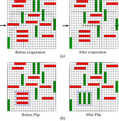
We study this system using constant grand canonical Monte Carlo simulations. The algorithm that we implement is an adaptation of the algorithm with cluster moves that was introduced in Refs. Kundu et al. (2013, 2012) to study the problem of hard rods (m=1). We describe the algorithm below. Given a valid configuration of rectangles, in a single move, a row or a column is chosen at random. If a row is chosen, then all horizontal rectangles whose heads (bottom, left corner) lie in that row are removed, leaving the rectangles with heads in other rows untouched. The emptied row now consists of two kinds of sites: forbidden sites that cannot be occupied with horizontal rectangles due to the presence of vertical rectangles in the same row or due to rectangles with heads in the neighboring rows, and sites that may be occupied by horizontal rectangles in a valid configuration. An example illustrating the forbidden sites is shown in Fig. 1(a). It is clear that the sites that may be occupied are divided into intervals of contiguous empty sites. The problem of occupation of the emptied row with a new configuration now reduces to the problem of occupying the empty intervals. However, the empty intervals may be occupied independent of each other, as the occupation of one is not affected by the configuration of rectangles in the remaining ones. Thus, the re-occupation of the emptied row reduces to a problem of occupying a one dimensional interval with rods. This problem is easily solvable and the equilibrium probabilities of each new configuration may be easily calculated. We refer to Refs. Kundu et al. (2013, 2012) for the calculation of these probabilities. If a column is chosen instead of a row, then a similar operation is performed for the vertical rectangles whose heads lie in that column.
In addition to the above evaporation-deposition move, we find that the autocorrelation time is reduced considerably by introducing a flip move. In this move, a site is picked at random. If it is occupied by the head of a horizontal rectangle, then we check whether sites are occupied by the heads of horizontal rectangles. If that is the case, we call this set of aligned rectangles a rotatable plaquette of horizontal rectangles. In the flip move such a rotatable plaquette of size , containing horizontal rectangles, is replaced by a similar plaquette of vertical rectangles. An example of the flip move is shown in Fig. 1(b). If is occupied by the head of a vertical rectangle and a rotatable plaquette of vertical rectangles is present, then it is replaced by a plaquette of aligned horizontal rectangles. A Monte Carlo move corresponds to evaporation–deposition moves and flip moves. It is easy to check that the algorithm is ergodic and obeys detailed balance.
We implement a parallelized version of the above algorithm. In the evaporation-deposition move, we simultaneously update all rows that are separated by . Once all rows are updated in this manner, the columns are updated. We also parallelize the flip move. The lattice is divided into blocks of size . The flipping of each of these blocks is independent of the other and may therefore be flipped simultaneously. We flip a rotatable plaquette with probability . The parallelization and efficiency of the algorithm allows us to simulate large systems (up to ) at high densities (up to ).
We check for equilibration by starting the simulations with two different initial configurations and making sure that the final equilibrium state is independent of the initial condition. One configuration is a fully nematic state, where all rectangles are either horizontal or vertical and the other is a random configuration where rectangles of both vertical and horizontal orientations are deposited at random.
III The Different Phases
Snapshots of the different phases that we observe in simulations are shown in Fig. 2. First is the low density isotropic (I) phase in which the rectangles have neither orientational nor translational order [see Fig. 2(c)]. Second is the nematic (N) phase in which the rectangles have orientational order but no translational order [see Fig. 2(d)] . In this phase, the mean number of horizontal rectangles is different from that of vertical rectangles. The third phase is the columnar (C) phase, having orientational order and partial translational order [see Fig. 2(e)]. In this phase, if majority of rectangles are horizontal (vertical), then their heads, or bottom left corners, preferably lie in rows (columns) that are separated by . Thus, it breaks the translational symmetry in the direction perpendicular to the orientation but not parallel to the orientation. Clearly, there are symmetric C phases. In this phase the rectangles can slide much more along one lattice direction. The fourth phase is the crystalline sublattice (S) phase with no orientational order [see Fig. 2(f)]. We divide the square lattice into sublattices by assigning to a site a label . The sublattice labeling for the case is shown in Fig. 2(a). In the S phase, the heads of the rectangles preferably occupy one sublattice, breaking translational symmetry in both the directions.
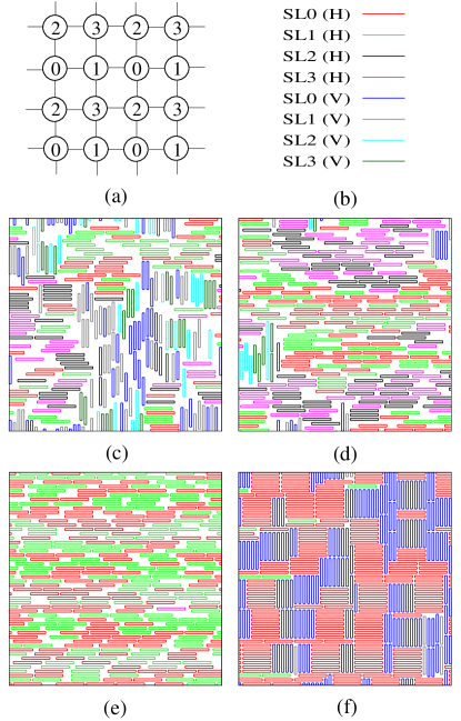
From the symmetry of the system we would expect up to phases. The orientational symmetry could be present or broken while the translational symmetry could be unbroken, broken along only one or both - and - directions. If the orientational symmetry is broken, then the translational symmetry could be broken either parallel or perpendicular to the preferred orientations. Out of the possibilities, we do not observe (i) a phase with no orientational order but partial translational order, (ii) a phase with orientational order and complete translational order (iii) a smectic like phase in which orientational order is present and translational symmetry parallel to the orientation is broken.
To distinguish among the four different phases we define the following order parameters:
| (1a) | |||||
| (1b) | |||||
| (1c) | |||||
| (1d) | |||||
where and are the total number of horizontal and vertical rectangles respectively, is the number of rectangles whose heads are in sublattice , are the number of rectangles whose heads are in row , and are the number of rectangles whose heads are in column . All four order parameters are zero in the I phase. is non-zero in the N and C phases, is non-zero in the C and S phases, is non-zero only in the C phase, and is non-zero only in the S phase. in Eq. (1d) has been defined for . Its generalization to is straightforward.
We now define the thermodynamic quantities that are useful to characterize the transitions between the different phases. ’s second moment , compressibility and the Binder cumulant are defined as
| (2a) | |||||
| (2b) | |||||
| (2c) | |||||
The transitions are accompanied by the singular behavior of the above thermodynamic quantities at the corresponding critical densities. Let , where is the critical chemical potential. The singular behavior is characterized by the critical exponents , , , defined by , , , , and , where is the correlation length, , and represents any of the order parameters. Only two exponents are independent, others being related to them through scaling relations.
The critical exponents , , and are obtained by finite size scaling of the different quantities near the critical point:
| (3a) | |||||
| (3b) | |||||
| (3c) | |||||
| (3d) | |||||
where , , , and are scaling functions.
IV Phase Diagram and Critical Behavior for
In this section, we discuss the phase diagram for the case and aspect ratio . The critical exponents characterizing the different continuous transitions are determined numerically.
IV.1 Phase Diagram
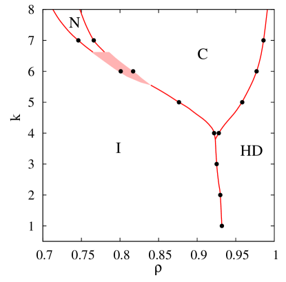
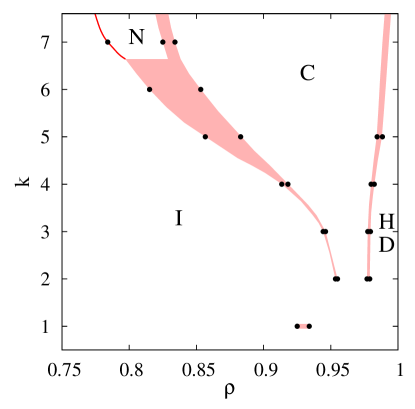
The phase diagram obtained from simulations for and integer are shown in Fig. 3. The low density phase is an I phase for all . The case is different from other . In this case, the problem reduces to a hard square problem and orientational order is not possible as there is no distinction between horizontal and vertical rectangles. The hard square system undergoes only one transition with increasing density, it being a continuous transition from the I phase to a C phase Baxter (1982); Bellemans and Nigam (1967); Pearce and Seaton (1988); Ramola and Dhar (2012). This transition belongs to the Ashkin Teller universality class (see Refs. Fernandes et al. (2007); Zhitomirsky and Tsunetsugu (2007); Feng et al. (2011); Ramola (2012) for recent numerical studies). For , we find that the system undergoes one continuous transition directly from the I phase to a crystalline S phase. On the other hand, the system with may exist in I, C, or S phases. With increasing density, the system undergoes two phase transitions: first from the I to a C phase which could be continuous or first order, and second, from the C to a S phase which is continuous. For , we observe three continuous transitions with increasing density: first from the I to the N phase, second into the C phase and third into the S phase. By confirming the existence of the N and C phases for , we expect the phase behavior for to be similar to that for .
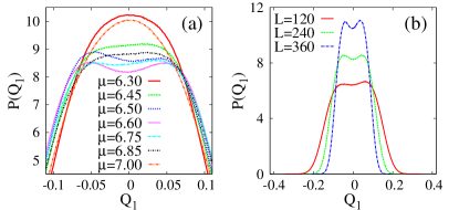
The system undergoes more than one transition only for . We now present some supporting evidence for this claim. In Fig. 4 (a) we show the probability distribution of the nematic order parameter , when , for different values of and fixed , close to the I-C and the C-S transitions. For lower values of , the distribution is peaked around zero corresponding to the I phase. With increasing , the distribution becomes flat and two symmetric maxima appear at ( also becomes nonzero simultaneously), corresponding to a C phase. On increasing further, the two maxima continuously merge into a single peak at =0, corresponding to the S phase ( also becomes zero and becomes nonzero). Fig. 4 (b) shows the distribution of for three different system sizes at a fixed value of for which has two symmetric maxima at . The two peaks become sharper and narrower with increasing . We find the similar behavior for also. From the above, we conclude that the C phase exists for albeit for a very narrow range of . For and we do not observe the existence of a columnar phase and find that the probability distributions of and are peaked around zero for all . Hence, we conclude that .
The N phase exists only for . This is also true for Ghosh and Dhar (2007). To see this, notice that the I-C transition for is first order (see Fig. 3). If a nematic phase exists for , then the first transition would have been continuous and in the Ising universality class Matoz-Fernandez et al. (2008a).
IV.2 Critical behavior for the isotropic-sublattice (I-S) phase transition
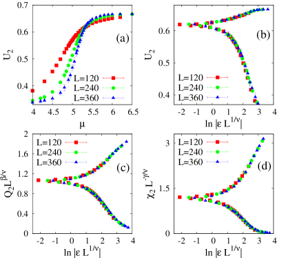
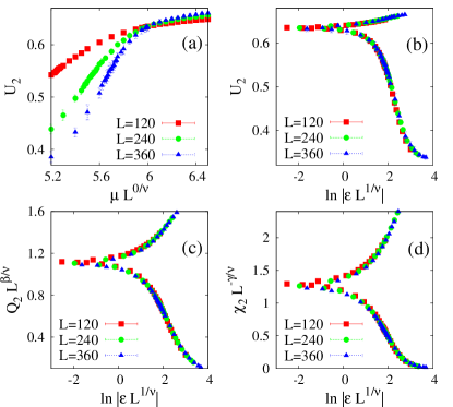
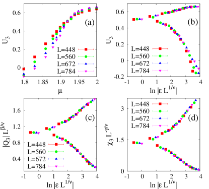
The system of rectangles with undergoes a direct I-S transition for . At this transition, the translational symmetry gets broken along both - and - direction but the rotational symmetry remains preserved. We study this transition using the order parameter [see Eq. (1b)]. is non-zero in the S phase and zero in the I phase. In this case and remains zero for all values of . The data collapse of , , and for different values of near the I-S transition are shown in Fig. 5 for and in Fig. 6 for . From the crossing of the Binder cumulant data for different , we estimate the critical chemical potential () for and () for . The order parameter increases continuously with from zero as is crossed, making the transition continuous. Since the phase has a four fold symmetry due to the four possible sublattices, we expect the transition to be in the Ashkin-Teller universality class. Indeed, we find a good collapse with and . Numerically, we find for and for . being larger than , we do not observe any divergence in . This transition could have also been studied using the order parameter .
.
IV.3 Critical behavior of the isotropic-columnar phase (I-C) transition
The I-C transition is seen for . When for , for the I-C and the C-S transitions are close to each other, making unsuitable for studying the critical behavior. We, therefore, study the I-C transition for ( rectangles) and ( rectangles).
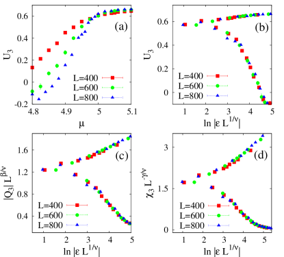
The critical behavior is best studied using the order parameter [see Eq. (1c)]. is non-zero only in the C phase. First, we present the critical behavior for . The simulation data for different system sizes are shown in Fig. 7. From the crossing of the Binder cumulant curves, we obtain (). The transition is found to be continuous. There are four possible columnar states: majority of heads are either in even or odd rows (when horizontal orientation is preferred), or in even or odd columns (when vertical orientation is preferred). Due to this four fold symmetry, we expect the I-C transition to be in the Ashkin-Teller universality class. The data for different collapse with , and (see Fig. 7), confirming the same. Unlike the I-S transition for , and lies between the Ising and q=4 Potts points. At the I-C transition partial breaking of translational symmetry and complete breaking of rotational symmetry occur simultaneously.
The I-C transition for is also continuous [see Fig. 4 (a)], and is therefore expected to be in the Ashkin-Teller universality class. However, there is no reason to expect that will be the same as that for .
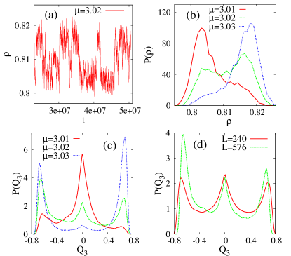
For , the I-C transition is surprisingly first order. Fig. 8(a) shows the time profile of density near the I-C transition. alternates between two well defined densities, one corresponding to the I phase and the other to the C phase. This is also seen in the probability distribution for density [see Fig. 8(b)]. Near the I-C transition it shows two peaks corresponding to the I and the C phases. Thus, at , the density has a discontinuity, which is shown by the shaded region in the phase diagram (see Fig. 3). The probability distribution of the order parameter shows similar behavior [see Fig. 8(c)]. Near the distribution shows three peaks: one at corresponding to the I phase and the other two at , corresponding to the C phase. At the three peaks become of equal height and the order parameter jumps from zero to a non-zero value. These peaks sharpen with increasing system size [see Fig. 8(d)]. These are typical signatures of a first order transition. Hence, we conclude that the I-C transition may be continuous or first order depending on .
IV.4 Critical behavior of the isotropic-nematic phase (I-N) transition
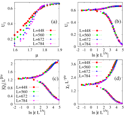
We find that the nematic phase exists only for . We study the I-N phase transition for using the order parameter [see Eq. (1a)]. is non-zero in the N and C phases and zero in the I phase. We confirm that the ordered phase is an N phase by checking that , which is non-zero only in the C phase, is zero. In the nematic phase the rectangles may choose either horizontal or vertical orientation. Thus, we expect the transition to be in the Ising universality class. When , this has been verified using extensive Monte Carlo simulations Matoz-Fernandez et al. (2008a). Here, we confirm the same for . The data for , and for different collapse onto one curve when scaled with the two dimensional Ising exponents , , and (see Fig. 9). We find (). We note that the value of at the point where the curves for different cross is slightly smaller than the Ising value . This suggests that larger system sizes are necessary for better collapse of the data.
IV.5 Critical behavior of the nematic-columnar phase (N-C) transition
The N-C transition is also studied for , using the order parameter . is zero in the nematic phase but nonzero in the columnar phase. At the I-N transition orientational symmetry gets broken. If the nematic phase consists of mostly horizontal (vertical) rectangles, then there is no preference over even and odd rows (columns). In the columnar phase the system chooses either even or odd rows (columns), once the orientational symmetry is broken. Due to the two broken symmetry phases we expect this transition to be in the Ising universality class. We indeed find good data collapse when , and for different system sizes are scaled with Ising exponents (see Fig. 10). The critical chemical potential or critical density is obtained from the crossing point of the binder cumulant for different . We find () for this transition. We expect the critical behavior to be same for .
IV.6 Critical behavior of the columnar-sublattice phase (C-S) transition
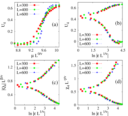
The C-S transition exists for . This transitions is studied by choosing . We characterize the C-S transition using the order parameter which is non zero only in the S phase. In the C phase the system chooses one particular orientation and either even or odd rows or columns, depending on the orientation. This corresponds to two sublattices being chosen among four of them. In the C-S transition the translational symmetry gets broken completely by choosing a particular sublattice, but along with that the orientational symmetry gets restored. This transition is found to be continuous. The data of , and for different near the C-S transition collapse well when scaled with the exponents belonging to the Ashkin-Teller universality class. The estimated critical exponents are , and (see Fig. 11). Binder cumulants for different system sizes cross at (). We expect similar behavior for and but possibly with different . The C-S transition occurs at very high density. With increasing , the relaxation time becomes increasingly large, making it difficult to obtain reliable data for the C-S transition when .
V Phase Diagram and Critical Behavior for
V.1 Phase diagram
The phase diagram that we obtain for , is shown in Fig. 12. When , the corresponding hard square system has a single, first order transition from the I phase into the C phase Fernandes et al. (2007). The shaded region between two points denotes a region of phase coexistence. For , the system undergoes two first order transitions with increasing density: first an I-C transition and second a C-S transition. This is unlike the case , where for and we find only one transition. For , we find three transitions as in the case. The first transition from I to N phase is continuous while the second from N to C phase appears to be first order. Although we cannot obtain reliable data for the third transition into the S phase, we expect it to be first order. We note that the minimum value of beyond which the nematic phase exists is for both and , and matches with that for Ghosh and Dhar (2007).
V.2 The isotropic-columnar phase (I-C) transition
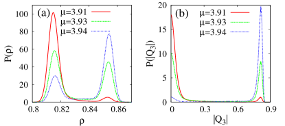
The I-C transition exists when . We study the this transition for , using the order parameter . Now there are six possible choices for the C phase: heads are predominantly in one of the rows or (mod ) with all the columns equally occupied (if horizontal orientation is preferred) or in one of the columns or (mod ) and all the rows are equally occupied (if vertical orientation is preferred). Making an analogy with the six state Potts model, we expect the I-C transition to be first order. The probability distribution of the density and the order parameter for near the I-C transition is shown in Fig. 13. The distributions are clearly double peaked at and near the transition point, one corresponding to the I phase and the other to the C phase. We find that these peaks become sharper with increasing system size. This is suggestive of a first order phase transition with a discontinuity in both density and order parameter as crosses . The discontinuity in the density is denoted by the shaded regions of Fig. 12. The chemical potential at which the I-C transition occurs is given by, . Similar behavior is seen near the I-C transition for rectangles of size with and . We observe that the discontinuity in the density increases with .
V.3 Critical behavior of the isotropic-nematic phase (I-N) transition
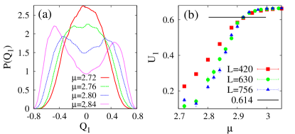
As for , for we find the existence of the nematic phase only for . We study the I-N transition for with the order parameter . It is expected to be in the Ising universality class since there are two possible choices of the orientation: either horizontal or vertical. We are unable to obtain good data collapse for , and as the relaxation time increases with increasing and . Instead, we present some evidence for the transition being continuous and belonging to the Ising universality class. In Fig. 14 (a), the distribution of the order parameter near the I-N transition is shown. The two symmetric peaks of the distribution come closer with decreasing and merge to a single peak, this being a signature of a continuous transition. The Binder cumulant for different system sizes cross at () [see Fig. 14 (b)]. The value of at is very close to the value () for the Ising universality class.
V.4 The nematic-columnar phase (N-C) transition
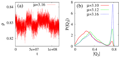
The N-C transition is studied for using the order parameter . Contrary to our expectation that the N-C transition should be in the q=3 Potts universality class, we observe a first order transition. The temporal dependence of the density near the N-C transition is shown in Fig. 15(a). Density jumps between two well separated values corresponding to the two different phases near the coexistence. Fig 15(b) shows the discontinuity in the order parameter near the transition. shows two peaks of approximately equal height near . However, we are limited in our ability to obtain reliable data for rectangles for larger system sizes, and the observed first order nature could be spurious.
V.5 The columnar-sublattice phase (C-S) transition
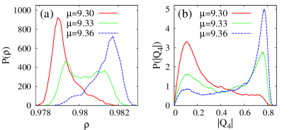
The C-S transition is studied by choosing . We use the order parameter which is nonzero only in the S phase. The probability distribution of the density and the order parameter for rectangles near the C-S transitions is shown in Fig. 16. The distributions are again double peaked at and near the transition point, making the C-S transition first order. These peaks become sharper with increasing system size. The discontinuity in the density near the C-S transition is very small and can also be seen in the shaded portions of Fig. 12. We estimate . Similar behavior near the C-S transitions is also observed for , but the relaxation time increases with .
VI Estimation of the phase boundaries using analytical methods
In this section we obtain the asymptotic behavior of the phase diagram for large using theoretical arguments.
VI.1 The isotropic–nematic phase boundary
The critical density for the I-N phase transition, for fixed and may be determined by making an analogy with the continuum problem. The limit , keeping fixed corresponds to the system of oriented lines in the continuum. For this problem Ghosh and Dhar (2007); Matoz-Fernandez et al. (2008b). The constant is estimated to be Ghosh and Dhar (2007); Matoz-Fernandez et al. (2008b). Thus, we expect , where is independent of . For , we observe only a weak dependence of on with the critical density being , and .
VI.2 The nematic–columnar phase boundary
To obtain the asymptotic behavior of the N-C phase boundary, we use an ad hoc Bethe approximation scheme for rods due to DiMarzio DiMarzio (1961), adapted to other shapes Sokolova and Tumanyan (2000). To estimate the phase boundary of the nematic–columnar transition of rectangles on the square lattice with sites, we require the entropy as a function of the occupation densities of the types of rows/columns. The calculations become much simpler, if we consider a fully oriented phase with only horizontal rectangles. Now, the nematic phase corresponds to the the phase where there is equal occupancy of each of the types of rows, while the columnar phase breaks this symmetry and preferentially occupies one type of row. For this simplified model with only one orientation, we estimate the entropy within an ad hoc Bethe approximation as detailed below. We present the calculation for , classifying the rows as even and odd rows. Generalization to higher values of is straight forward.
Let there be () number of rectangles whose heads (left bottom site of the rectangle) occupy even (odd) rows. We first place the rectangles one by one on the even rows. Given that rectangles have already been placed, the number of ways in which the rectangle can be placed may be estimated as follows. The head of the rectangle has to be placed on an empty site of an even row. We denote this site by (see Fig. 17). The site can be chosen at random in () ways, being the number of sites in even rows and being the number of occupied sites in the even rows by the rectangles. We now require that the consecutive sites to the right of are also empty. The probability of this being true is , where is the conditional probability that (see Fig. 17) is empty given that is empty. In terms of and , is given by
| (4) |

To place the rectangle, we also require that the site (see Fig. 17) and the consecutive sites to the right of are also empty. The probability of this being true is , where is the conditional probability that is empty given is empty, and is the conditional probability that (see Fig. 17) is empty given that both and are empty. Sites C and D belongs to an odd row. Since both A and B are empty, C and D can be occupied only by rectangles with heads in the same odd row. But, there are no such rectangles. Therefore, , and . Thus, given that rectangles have been placed, the rectangle may be placed in
| (5) |
ways. Hence, the total number of ways of placing rectangles with heads on even rows is
| (6) | |||||
Keeping the rectangles with heads on even rows, we now place rectangles one by one on the odd rows. Given that rectangles have been placed on the odd rows, the number of ways of placing the rectangle may be estimated as follows. The head of the rectangle must be placed on an empty site on an odd row. We denote this site by (see Fig. 17). may be chosen in ways, where we have ignored correlations between rectangles. Here is the number of occupied sites in the odd rows due to the rectangles on the even rows, and the is the number of sites occupied by rectangles in odd rows. We now require that the consecutive sites to the right of are also empty. The probability of this being true is , where is the conditional probability that (see Fig. 17) is empty given that is empty. is given by
| (7) |
where we have again ignored all correlations.
For placing the rectangle, we also require that the site (see Fig. 17) and the consecutive sites to the right of are also empty. The probability of this being true is , where is the conditional probability that is empty given is empty, and is the conditional probability that (see Fig. 17) is empty given that both and are empty. Ignoring correlations, is given by
| (8) |
If we calculate following the procedure developed by DiMarzio in Ref. DiMarzio (1961), then the resultant entropy is not symmetric with respect to and and depends on the order of placement. To overcome this shortcoming, we follow the Bethe approximation proposed in Ref. Sokolova and Tumanyan (2000) as follows:
| (9) | |||||
| (10) |
where in Eq. (9), we used and in Eq. (10), we replaced by , which is an approximation.
In Eq.(10), from symmetry, it is easy to see that and and can be read off from Eqs. (7) and (8). To obtain an expression for , the probability that is empty, given that the site is empty, we again ignore correlations. We then obtain
| (11) |
The number of ways of placing the rectangle is
| (12) | |||||
Substituting for each of the quantities on the right hand side, we obtain the total number of ways of placing the rectangles on the odd rows as
| (13) | |||||
We would like to express the entropy in terms of the total density and the densities of occupied sites in even and odd rows, given by and respectively. Clearly,
| (14) | |||||
| (15) | |||||
| (16) |
The entropy per site in the thermodynamic limit is given by
| (17) |
Substituting for and from Eqs. (6) and (13), we obtain
| (18) | |||||
We express the entropy in terms of density and the order parameter , defined as
| (19) |
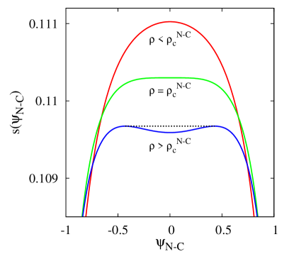
is zero in the nematic phase and non-zero in the columnar phase. For a fixed value of , the equilibrium values of and are determined by maximizing the entropy with respect to . In Fig. 18 we show the variation of entropy with for different densities. For small values of , the entropy is maximized by , , . Beyond a critical density , is maximized by , , . grows continuously with for , and thus the transition for is continuous.
The expansion of in powers of has only even powers of since is invariant when . Thus, the critical density is obtained from the condition . This gives
| (20) | |||||
where . We note that as , tends to a independent value and that the transition exists for all .
We can similarly calculate the entropy for and then generalize the expression of entropy for arbitrary and . Now, there are densities , , , , corresponding to the types of rows. In terms of them, the entropy is given by
| (21) | |||||
Here, we define the order parameter to be
| (22) |
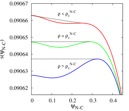
where we set . Now, is not invariant when . Thus, when expanded in powers of , has cubic terms, making the transition first order. This is illustrated in Fig. 19 which shows the variation of entropy with for different near the N-C transition. For low densities exhibit a single peak at , but with increasing a secondary maximum gets developed at . For the maximum at and becomes of equal height. Beyond the global maximum of jumps to , making the N-C transition to be first order.
Unlike the case, there is no way to obtain an analytic expression for . For m=3, the numerically determined for different is shown in Fig. (20). From the data, we obtain
| (23) |
We note that this expression has the same form as for [see Eq. (20)].
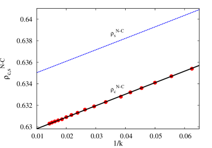
For , we proceed as follows. The transition density is bounded from above by the spinodal density , the density at which the entropy at changes from a local maximum to local minimum. is obtained from the condition and we obtain
| (24) | |||||
| (25) | |||||
| (26) |
where and . The spinodal density is compared with in Fig. 20. From Eq. (26), it follows that and tends to one when . The limit corresponds to the continuum limit. In this limit . Thus, it is not clear whether the nematic-columnar phase transition will exist in the continuum.
VI.3 The columnar–sublattice phase boundary
The dependence of the C-S phase boundary on and may be determined by estimating the entropy for the C and S phases close to full packing. We approximate the entropy of the C phase by the entropy of the fully aligned C phase. Since the heads of the rectangles are all in either even or odd rows/columns, by ignoring the unoccupied rows/columns, the calculation of entropy reduces to an one dimensional problem of rods. The mean number of holes in a row is , and the mean number of rods (of length ) in a row is . There are such rows. The number of ways of arranging the rods and holes on a row is
| (27) |
such that the total number of ways of arranging the rectangles is . Hence, , the entropy per site of the columnar phase is given by , which for densities close to is
| (28) |
We now estimate the entropy for the sublattice phase. At full packing, the head of each rectangle is on one of sublattices. Ignoring the sites belonging to other sublattices, it is easy to see that each configuration of rectangles can be mapped on to a configuration of rods of length on a lattice of size . When , by solving the full packed problem of rods on strips, it is known that the entropy per unit site is Ghosh and Dhar (2007). For rectangles of size we obtain
| (29) |
where is the entropy per site of the S phase. For densities close to 1 () we estimate the correction term to by removing fraction of rectangles at random from the fully packed state. Here, we ignore the entropy of the holes, assuming that the holes form bound states. This gives the entropy of the sublattice phase, close to the full packing to be approximately
| (30) |
Comparing Eqs. (28) and (30) up to the leading order we obtain the critical density for the C-S transition to be
| (31) |
where is a constant.
Given the above asymptotic behavior of the phase boundaries, we expect that the phase diagram for will be similar to that obtained for for large . For small , we check that for rectangles of size , there are two transitions just as in rectangles. Thus, we are led to conjecture that the phase diagram for will be qualitatively similar to that for for all .
VII Summary and Discussion
To summarize, we obtained the rich phase diagram of a system of hard rectangles on a square lattice for integer using a combination of Monte Carlo simulations and analytical calculations. We improve an existing cluster Monte Carlo algorithm by implementing the plaquette flip move, which reduces the autocorrelation time considerably. For , we show that the system undergoes three entropy driven transitions with increasing density. For , we find that the I-N, N-C and C-S transitions are continuous, but the I-C transition may be continuous or first order, depending on . The critical exponents for the continuous transitions were obtained using finite size scaling. The I-N and N-C transitions are found to be in the Ising universality class, while the C-S transition in the Ashkin-Teller universality class. The I-C transitions are also found to be in the Ashkin-Teller universality class when continuous. For larger , the number of possible ordered states increase and the corresponding transitions become first order.
Surprisingly, our numerical data suggests that the nematic–columnar phase transition for is first order. However, once a nematic phase with orientational order exists, there are only three possible choices for the columnar phase. By analogy with the three state Potts model, we would expect a continuous transition, in contradiction with the numerical result. We also performed simulations for a system where the activity for vertical rectangles is zero (only horizontal rectangles are present) and observed again a first order transition. However, for rectangles, the autocorrelation time is high and it becomes increasingly difficult to obtain reliable data. Simulations of larger systems are required to resolve this puzzle in the future.
When , the I-C transition is found to be continuous for and , but first order for . For , it is a weak first order transition and it is difficult to see the jump in density for small system sizes. It is also possible that the data is difficult to interpret because the transition point is close to a triciritcal point (the intersection of the I-N and N-C phase boundaries). It would be interesting to reconfirm the first order nature by either simulating larger systems or doing constant density Monte Carlo simulations at the transition point so that phase separation may be seen. Also, determining a method to map and to the Ashkin Teller model parameters would be useful in clarifying this issue.
Another issue that we are not able to resolve completely is the determination of the minimum value of (say ) for which two transitions exist. For , we show that . When , our numerical data suggests that , with a direct transition from isotropic to sublattice phase for . However, for , the columnar phase exists in a very narrow window of or . Whether the columnar phase is present for , but we are unable to resolve the transitions, is something that requires investigation of much larger system sizes.
We obtained the N-C phase boundary analytically through a Bethe approximation. However, an improvement of the calculations is desirable as the approximations are ad hoc and uncontrolled and there does not appear to be a systematic way of improving it. An exact solution on tree like lattices, for example the random locally layered tree like lattice (RLTL) Dhar et al. (2011); Kundu and Rajesh (2013) would be more satisfying. At present, we have not been able to formulate the problem of rectangles on RLTL. This is a promising area for future study.
Several extensions of the problem are possible. An interesting limit is the continuum problem of oriented rectangles of aspect ration . This corresponds to the limit of the lattice model. From the analytical arguments presented in the paper, we would expect a isotropic nematic transition at a critical density proportional to . Within the Bethe approximation, the spinodal density for the nematic–columnar transition tends to in the continuum limit. This being an upper bound for the critical density for the nematic–columnar transition, it is likely that the continuum problem will have a second transition into a columnar like phase, a true columnar phase being prohibited by the Mermin Wagner theorem. We expect the C-S transition to be absent in the continuum, as the critical density for the C-S transition tends to as . It would be interesting to verify these claims numerically. Preliminary simulations show an isotropic nematic transition.
One could also consider the model on other lattices like the triangular lattice. Here, the parallelograms may orient themselves along three possible lattice directions. For each orientation the rectangles may have two different slants (as the shorter side of the rectangle may be oriented along two possible lattice directions). In this case, we expect the phase diagram to be qualitatively similar to that for the square lattice. However, as there are three broken symmetry phases corresponding to the three directions, the I-N transition would be in the 3 state Potts universality class, as opposed to Ising universality class for the square lattice. However, the N-C transition would be same as that for the square lattice. The I-C transition is now expected to be first order for all since the number of symmetric C phases increases from to . The S phase will now have symmetric states, the extra factor of being due to the two different slants corresponding to each orientation. Therefore, we expect the I-S transition to be always first order. It would be interesting to study the C-S transition carefully in detail for the triangular lattice and compare with that for the square lattice.
We have also studied systems with non-integer on the square lattice (e.g., ). Now, it is straightforward to see that the high density phase cannot have sublattice order. Thus, the high density phase does not possess either translational or orientational order. But, at intermediate densities, we observe the existence of the C phase for and N phase for . When we observe the C phase for (rectangles of size ). In this case the I-C transition is found to be first order. For both and , the I-N and N-C transitions are expected to be similar to that for integer . Unlike integer , we do not observe any transition for small ( for ) and the phase remains isotropic at all densities. We hope to clarify these issues in detail in a future paper.
We argued, based on an analogy with the continuum problem, that , where is independent of . Can this conjecture be verified analytically or through numerical simulations? We expect that for , the critical density can be determined numerically up to a large enough to determine . Comparison with the value of for Ghosh and Dhar (2007); Matoz-Fernandez et al. (2008b) would help in verifying the conjecture.
Extension to three dimensional cubic lattice would result in a much richer phase diagram that remains to be explored. The algorithm used in this paper is easily implementable in three dimensions.
Finally, the case (hard rods) is the only instance where the existence of a nematic phase may be proved rigorously Disertori and Giuliani (2013). To the best of our knowledge, there exists no proof of existence of phases with partial translational order like the columnar phase. The hard rectangle model seems an ideal candidate to prove its existence.
Acknowledgements.
We thank Deepak Dhar and Jürgen F. Stilck for helpful discussions. The simulations were carried out on the supercomputing machine Annapurna at The Institute of Mathematical Sciences.References
- Onsager (1949) L. Onsager, Ann. N.Y. Acad. Sci. 51, 627 (1949).
- Flory (1956) P. J. Flory, Proc. R. Soc. 234, 73 (1956).
- de Gennes and Prost (1995) P. G. de Gennes and J. Prost, The Physics of Liquid Crystals (Oxford University Press, Oxford, 1995) pp. 64–66.
- Vroege and Lekkerkerker (1992) G. J. Vroege and H. N. W. Lekkerkerker, Rep. Prog. Phys. 55, 1241 (1992).
- Dhar et al. (2011) D. Dhar, R. Rajesh, and J. F. Stilck, Phys. Rev. E 84, 011140 (2011).
- Frenkel et al. (1988) D. Frenkel, H. N. W. Lekkerkerker, and A. Stroobants, Nature 332, 822 (1988).
- Bolhuis and Frenkel (1997) P. Bolhuis and D. Frenkel, J. Chem. Phys 106, 666 (1997).
- Straley (1971) J. P. Straley, Phys. Rev. A 4, 675 (1971).
- Frenkel and Eppenga (1985) D. Frenkel and R. Eppenga, Phys. Rev. A 31, 1776 (1985).
- Wojciechowski and Frenkel (2004) K. W. Wojciechowski and D. Frenkel, Comput. Methods Sci. Tech. 10, 235 (2004).
- Khandkar and Barma (2005) M. D. Khandkar and M. Barma, Phys. Rev. E 72, 051717 (2005).
- Donev et al. (2006) A. Donev, J. Burton, F. H. Stillinger, and S. Torquato, Phys. Rev. B 73, 054109 (2006).
- Zhao et al. (2007) K. Zhao, C. Harrison, D. Huse, W. B. Russel, and P. M. Chaikin, Phys. Rev. E 76, 040401 (2007).
- Vink (2009) R. L. C. Vink, Euro. Phys. J. B 72, 225 (2009).
- Fraden et al. (1989) S. Fraden, G. Maret, D. L. D. Caspar, and R. B. Meyer, Phys. Rev. Lett. 63, 2068 (1989).
- Islam et al. (2004) M. F. Islam, A. M. Alsayed, Z. Dogic, J. Zhang, T. C. Lubensky, and A. G. Yodh, Phys. Rev. Lett. 92, 088303 (2004).
- Zhao et al. (2011) K. Zhao, R. Bruinsma, and T. G. Mason, Proc. Natl. Acad. Sci. 108, 2684 (2011).
- Ghosh and Dhar (2007) A. Ghosh and D. Dhar, Euro. Phys. Lett. 78, 20003 (2007).
- Disertori and Giuliani (2013) M. Disertori and A. Giuliani, Commun. Math. Phys. 323, 143 (2013).
- Kundu et al. (2013) J. Kundu, R. Rajesh, D. Dhar, and J. F. Stilck, Phys. Rev. E 87, 032103 (2013).
- Matoz-Fernandez et al. (2008a) D. A. Matoz-Fernandez, D. H. Linares, and A. J. Ramirez-Pastor, Euro. Phys. Lett 82, 50007 (2008a).
- Fischer and Vink (2009) T. Fischer and R. L. C. Vink, Euro. Phys. Lett. 85, 56003 (2009).
- Kundu and Rajesh (2013) J. Kundu and R. Rajesh, Phys. Rev. E 88, 012134 (2013).
- Baxter (1982) R. J. Baxter, Exactly Solved Models in Statistical Mechanics (Academic Press, London, 1982).
- Fernandes et al. (2007) H. C. M. Fernandes, J. J. Arenzon, and Y. Levin, J. Chem. Phys. 126, 114508 (2007).
- Zhitomirsky and Tsunetsugu (2007) M. E. Zhitomirsky and H. Tsunetsugu, Phys. Rev. B 75, 224416 (2007).
- Feng et al. (2011) X. Feng, H. W. J. Blöte, and B. Nienhuis, Phys. Rev. E 83, 061153 (2011).
- Ramola (2012) K. Ramola, Onset of Order in Lattice Systems: Kitaev Model and Hard Squares, Ph.D. thesis, Tata Institute of Fundamental Research, Mumbai (2012).
- Zwanzig (1963) R. Zwanzig, J. Chem. Phys. 39, 1714 (1963).
- Heilmann and Lieb (1970) O. J. Heilmann and E. H. Lieb, Phys. Rev. Lett. 24, 1412 (1970).
- Kunz (1970) H. Kunz, Phys. Lett. A 32, 311 (1970).
- Gruber and Kunz (1971) C. Gruber and H. Kunz, Commun. Math. Phys. 22, 133 (1971).
- Heilmann and Lieb (1972) O. J. Heilmann and E. Lieb, Commun. Math. Phys. 25, 190 (1972).
- Barnes et al. (2009a) B. C. Barnes, D. W. Siderius, and L. D. Gelb, Langmuir 25, 6702 (2009a).
- Casey and Harrowell (1995) A. Casey and P. Harrowell, J. Chem. Phys. 103, 6143 (1995).
- Patrykiejew et al. (2000) A. Patrykiejew, S. Sokolowski, and K. Binder, Surf. Sci. Rep. 37, 207 (2000).
- Taylor et al. (1985) D. E. Taylor, E. D. Williams, R. L. Park, N. C. Bartelt, and T. L. Einstein, Phys. Rev. B 32, 4653 (1985).
- Bak et al. (1985) P. Bak, P. Kleban, W. N. Unertl, J. Ochab, G. Akinci, N. C. Bartelt, and T. L. Einstein, Phys. Rev. Lett. 54, 1539 (1985).
- Clarke et al. (2000) N. Clarke, J. A. Cuesta, R. Sear, P. Sollich, and A. Speranza, J. Chem. Phys 113, 5817 (2000).
- Martínez-Ratón and Cuesta (2003) Y. Martínez-Ratón and J. A. Cuesta, J. Chem. Phys 118, 10164 (2003).
- van Roij et al. (2000) R. van Roij, M. Dijkstra, and R. Evans, Euro. Phys. Lett. 49, 350 (2000).
- Ramirez-Pastor et al. (1999) A. J. Ramirez-Pastor, T. P. Eggarter, V. D. Pereyra, and J. L. Riccardo, Phys. Rev. B 59, 11027 (1999).
- Romá et al. (2003) F. Romá, A. J. Ramirez-Pastor, and J. L. Riccardo, Langmuir 19, 6770 (2003).
- Bellemans and Nigam (1967) A. Bellemans and R. K. Nigam, J. Chem. Phys. 46, 2922 (1967).
- Pearce and Seaton (1988) P. A. Pearce and K. A. Seaton, J. Stat. Phys. 53, 1061 (1988).
- Ramola and Dhar (2012) K. Ramola and D. Dhar, Phys. Rev. E 86, 031135 (2012).
- Baxter (1980) R. J. Baxter, J. Phys. A 13, L61 (1980).
- Heilmann and Praestgaard (1973) O. J. Heilmann and E. Praestgaard, J. Stat. Phys 9, 23 (1973).
- Dickman (2012) R. Dickman, J. Chem. Phys. 136, 174105 (2012).
- Verberkmoes and Nienhuis (1999) A. Verberkmoes and B. Nienhuis, Phys. Rev. Lett. 83, 3986 (1999).
- Kundu et al. (2012) J. Kundu, R. Rajesh, D. Dhar, and J. F. Stilck, AIP Conf. Proc. 1447, 113 (2012).
- Matoz-Fernandez et al. (2008b) D. A. Matoz-Fernandez, D. H. Linares, and A. J. Ramirez-Pastor, J. Chem. Phys. 128, 214902 (2008b).
- DiMarzio (1961) E. DiMarzio, J. Chem. Phys. 35, 658 (1961).
- Sokolova and Tumanyan (2000) E. P. Sokolova and N. P. Tumanyan, Liq. Crys. 27, 813 (2000).