Well-Posed Bayesian Geometric Inverse Problems Arising in Subsurface Flow

Abstract

In this paper, we consider the inverse problem of determining the permeability of the subsurface from hydraulic head measurements, within the framework of a steady Darcy model of groundwater flow. We study geometrically defined prior permeability fields, which admit layered, fault and channel structures, in order to mimic realistic subsurface features; within each layer we adopt either constant or continuous function representation of the permeability. This prior model leads to a parameter identification problem for a finite number of unknown parameters determining the geometry, together with either a finite number of permeability values (in the constant case) or a finite number of fields (in the continuous function case). We adopt a Bayesian framework showing existence and well-posedness of the posterior distribution. We also introduce novel Markov Chain-Monte Carlo (MCMC) methods, which exploit the different character of the geometric and permeability parameters, and build on recent advances in function space MCMC. These algorithms provide rigorous estimates of the permeability, as well as the uncertainty associated with it, and only require forward model evaluations. No adjoint solvers are required and hence the methodology is applicable to black-box forward models. We then use these methods to explore the posterior and to illustrate the methodology with numerical experiments.

1 Introduction

Quantification of uncertainty in the geologic properties of the subsurface is essential for optimal management and decision-making in subsurface flow applications such as nuclear waste disposal, geologic storage of CO₂ and enhanced-oil-recovery. The environmental impact of these applications, for example, cannot be properly assessed without quantifying the uncertainty in geologic properties of the formation. However, typical uncertainty of a priori geologic information often results in large uncertainty in the flow predictions. This uncertainty is, in turn, detrimental to optimally managing the process under consideration. A common strategy to reduce uncertainty and improve our ability to make decisions is to incorporate (or assimilate) data, typically corrupted by noise, that arise from the flow response to the given geologic scenario. Because of the prior uncertainty in geological information, and because of the noise in the data, this assimilation of data into subsurface flow models is naturally framed in a Bayesian fashion: the aim is to characterize the posterior (conditional) probability of geologic properties given the observed data [36] . The Bayesian framework is therefore a statistical approach for solving the inverse problem of identifying unknown geologic parameters given noisy data from the flow model. However, in contrast to deterministic approaches, the Bayesian framework provides a quantification of the uncertainty via the posterior; this in turn allows an assessment of the uncertainty arising in the corresponding model predictions. The goal of this paper is to study a class of inverse problems, arising in subsurface flow, in which both the geometry and the physical characteristics of the formation are to be inferred, and to demonstrate how the full power of the Bayesian methodology can be applied to such problems. We study existence and well-posedness of the posterior distribution, describe Markov Chain-Monte Carlo (MCMC) methods tailored to the specifics of the problems of interest, and show numerical results based on this methodology. We work within the context of a steady single-phase Darcy flow model, but the mathematical approach, and resulting algorithms, may be employed within more complex subsurface flow models.

1.1 Literature Review: Computational and Mathematical Setting

The first paper to highlight the power of the Bayesian approach to regularization of inverse problems is [16], where linear inverse problems, including heat kernel inversion, were discussed. The theory of Bayesian inversion for linear problems was then further developed in [32, 29] whilst the book [23] demonstrated the potential of the approach for a range of complex inverse problems, linear and nonlinear, arising in applications. Alongside these developments was the work of Lasanen which lays the mathematical foundations of Bayesian inversion for a general class of nonlinear inverse problems [25, 26, 27]. The papers [33, 34] demonstrate approximation results for the posterior distribution, employing Kullback-Leibler divergence and total variation metric respectively, for finite dimensional problems. The paper [39] demonstrated how the infinite dimensional perspective on Bayesian inversion leads to a well-posedness and approximation theory, and in particular to the central role played by the Hellinger metric in these results. The papers [5, 6, 11] demonstrated application of these theories to various problems arising in fluid mechanics and in subsurface flow. Most of this work stemming from [39] concerns the use of Gaussian random field priors and is hence limited to the reconstruction of continuous fields or to fields with discontinuous properties where the positions of the discontinuities are known and can be built in explicitly, through the prior mean, or through construction of the inverse covariance operators as in [22]. The article [28] introduced Besov priors in order to allow for the solution of linear inverse problems arising in imaging where edges and discontinuities are important and this work was subsequently partially generalized to nonlinear inverse problems arising in subsurface flow [10]. However none of this work is well-adapted to the geometrical discontinuous structures observed in subsurface formations, where layers, faults and channels may arise. In this paper we address this by formulating well-posed nonlinear Bayesian inverse problems allowing for such structures.

The computational approach highlighted in [23] is based primarily on the “discretize first then apply algorithm” approach with, for example, MCMC methods used as the algorithm. The work highlighted in [8] shows the power of an approach based on “apply algorithm then discretize”, leading to new MCMC methods which have the advantage of having mixing rates which are mesh-independent [19, 40]; the importance of mesh-independence is also highlighted in the work [28]. However the work overviewed in [8] is again mainly aimed at problems with Gaussian priors. In this paper we build on this work and develop MCMC methods which use Metropolis-within-Gibbs methodologies to separate geometric and physical parameters within the overall MCMC iteration; furthermore these MCMC methods require only solution of the forward problem and no linearizations of the forward operator, and are hence suitable in situations where no adjoint solvers are available and only black-box forward simulation software is provided. We use the resulting MCMC methodology to solve some hard geometric inverse problems arising in subsurface modelling.

1.2 Literature Review: Subsurface Applications

While standard approaches for data assimilation in subsurface flow models are mainly based on the Bayesian formalism, most of those approaches apply the Bayesian framework to the resulting finite-dimensional approximation of the model under consideration [36]. However, recent work [20] has shown the potential detrimental effect of directly applying standard MCMC methods to approximate finite-dimensional posteriors which arise from discretization of PDE based Bayesian inverse problems. For standard subsurface flow models, the forward (parameter-to-output) map is nonlinear, and so even if the prior distribution is Gaussian, the posterior is in general non-Gaussian. Therefore, the full characterization of the posterior can only be accomplished by sampling methods such as Markov Chain Monte Carlo (MCMC). On the other hand, unknown geologic properties are in general described by functions that appear as coefficients of the PDE flow model. Then, the Bayesian posterior of these discretized functions is defined on a very high-dimensional space (e.g $10^{5}\sim 10^{6}$) and sampling with standard MCMC methods [15, 30] becomes computationally prohibitive. Some standard MCMC approaches avoid the aforementioned issue by parametrizing the unknown geologic properties in terms a small number of parameters (e.g. $10\sim 20$) [14, 34]. Some others, however, consider the full parameterization of the unknown (i.e. as a discretized function) but are only capable of characterizing posteriors from one-dimensional problems on a very coarse grids [15, 30]. While the aforementioned strategies offer a significant insight into to the solution of Bayesian inverse problems in subsurface models, there remains substantial opportunity for the improvement and development of Bayesian data assimilation techniques capable of describing the posterior distributions accurately and efficiently, using the mesh-independent MCMC schemes overviewed in [8] and applied to subsurface applications in [20]. In particular we aim to do so in this paper in the context of geometrically defined models of the geologic properties.

The petrophysical characterization of complex reservoirs involves the identification of the geologic facies of the formation. For those complex geologies, prior knowledge may include uncertain information of the interface between the geologic facies as well as the spatial structure of each of the rock types. In addition, prior knowledge of complex reservoirs may also include information of potential faults. Moreover, if the depositional environment is known a priori, then geometrical shapes that characterize the petrophsyical properties of the formation may constitute an integral part of the prior information. Whenever the aforementioned information is part of the prior knowledge, the conditioning or assimilation of data should accommodate the geologic data provided a priori. This can be accomplished with the proper parameterization of the geologic properties so that different facies are honored. In [24] for example, a channelized structure was parameterized with a small number of unknowns and a deterministic history matching (data assimilation) was conducted on a two-phase flow model. More sophisticated parameterization of geologic facies involves the level-set approach for history matching used by [13, 21] in a deterministic framework. Recently, in [41] the level-set approach is combined with the Bayesian framework to provide a characterization of the posterior. This Bayesian application is constructed on the finite-dimensional approximation of the flow-model and is therefore subject to the computational limitations previously indicated, namely mesh-dependent convergence properties. While the work of [41] provides an upscaling to provide computational feasibility, the computations reported involved a limited number of samples, potentially insufficient for the proper characterization of the Bayesian posterior.

There are also several facies estimation approaches based on ad hoc Gaussian approximations of the posterior. For example, in [31] a pluri-Gaussian model of the geologic facies was used with an ensemble Kalman filter (EnKF) approach to generate an ensemble of realizations. In [42] a randomized likelihood method was used to estimate the parameters characterized with channels. In [4] a level-set approach was used with EnKF to generate an ensemble of updated facies. Although the aforementioned implementations are computationally feasible and may recover the truth within credible intervals (Bayesian confidence intervals), the methods may provide uncontrolled approximations of the posterior. Even for simple Gaussian priors, in [20] numerical evidence has been provided of the poor characterization that ensemble methods may produce when compared to a fully resolved posterior.

It is also worth mentioning the recent work of [3] where the Bayesian framework was used for facies identification in petroleum reservoirs. This work considers a parametrization of the geologic facies in terms of piecewise constant permeabilities on a multiphase-flow model. The paper demonstrates the need to properly sample multi-modal posterior distributions for which the standard ensemble-based methods will perform poorly.

1.3 Contribution of This Work

We develop a mathematical and numerical framework for Bayesian inversion to identify geometric and physical parameters of the permeability in a steady Darcy flow model. The geometric parameters aim at characterizing the location and shape of regions where discontinuities in the permeability arise due to the presence of different geologic facies. The physical parameters represent the spatial (usually continuous) variability of the permeability within each of the geologic facies that constitute the formation. We make three primary contributions: (i) we demonstrate the existence of a well-posed posterior distribution on the geometric and physical parameters including both piecewise constant (finite dimensional) and piecewise continuous (infinite dimensional) representations of the physical parameters; (ii) we describe appropriate MCMC methods which respect both the geometry and the possibly infinite dimensional nature of the physical parameters and which require only forward flow solvers and not the adjoint; (iii) we exhibit numerical studies of the resulting posterior distributions.

Clearly piecewise continuous fields will be able to represent more detailed features within the subsurface than piecewise constant ones. On the other hand we expect that piecewise constant fields will lead to simpler Bayesian inference, and in particular to speed-up of the Markov chains. There is hence a trade-off between accuracy and efficiency within geometric models of this type. The decision about which model to use will depend on the details of the problem at hand and in particular the quantities of interest under the posterior distribution. For this reason we study both piecewise continuous and piecewise constant fields.

Continuity of the forward mapping from unknown parameters to data, which is a key ingredient in establishing the existence of the posterior distribution [39], is not straightforward within classic elliptic theories based on $L^{\infty}$ permeabilities, because small changes in the geometry do not induce small changes in $L^{\infty}$. Nonetheless, one can prove that the forward mapping is continuous with respect to the unknown parameters, which allows us to show that the posterior distribution is well-defined. Furthermore, well-posedness of the inverse problem is established, namely continuity of the posterior distribution in the Hellinger and total variation metrics, with respect to small changes in the data. In the piecewise constant case, for log-normal and uniform priors on the values of the permeability, the data to posterior mapping is Lipschitz in these metrics, whilst for exponential priors it is Hölder with an exponent less than $1/2$ (resp. $1$) in the Hellinger (resp. total variation) metrics; problems for which the dependence is Hölder but not Lipschitz have not been seen in the examples considered to date, such as those in [39], and hence this dependence is interesting in its own right and may also have implications for the rate of convergence of numerical approximations. In the case of log-normal permeability field, the posterior is Lipschitz continuous with respect to data in both of these metrics. A novel Metropolis-within-Gibbs method is introduced in which proposals are made which are prior-reversible, leading to an accept-reject determined purely by the likelihood (or model-data mismatch) hence having clear physical interpretation, and in which the geometric and physical parameters are updated alternately, within the Gibbs framework. Finally some numerical examples are presented, for both multiple layers and fault models, demonstrating the feasibility of the methodology. We develop a rigorous application of the Bayesian framework for the estimation of geologic facies parametrized with small number of parameters, together with a finite or infinite dimensional set of physical parameters within each of the facies. Regarding the geometry we consider a general class of problems that includes stratified reservoirs with a potential fault, similar to the model used in [3]. In addition, we consider a simple channelized structure parameterized with small number of parameters, similar to the one described in [24].

The content of this paper is organized as follows. In Section 2, we provide a simplified description of the the forward model, with piecewise continuous permeabilities, and prove the continuity of the forward and observation map with respect to the geometric and physical parameters. Section 3 is devoted to the resulting Bayesian inverse problem from the geometric and physical parameters. The prior model is built both for the geometry and the values of permeability. We then show that the posterior measure is well defined and prove well-posedness results with respect to the data under this prior modeling. In Section 4, we introduce the novel Metropolis-within-Gibbs MCMC method to probe the posterior distribution. Some numerical results are shown in Section 5 to illustrate the effectiveness of the proposed methods.

2 Forward Model

In this section we introduce the subsurface flow model that we employ for application of the Bayesian framework. In subsection 2.1 we describe the underlying Darcy flow PDE model, in subsection 2.2 we introduce the family of geometrically defined permeabilities employed within the PDE and in subsection 2.3 we describe the observation model and the permeability to data map.

2.1 Darcy Flow Model

We are interested in characterizing the geologic properties of an aquifer whose physical domain is denoted by $D$. We assume that $D$ is a bounded open subset of $\mathbb{R}^{2}$ with Lipschitz boundary $\partial D$. We define the Hilbert spaces $H:=(L^{2}(D),\langle\cdot,\cdot\rangle,\|\cdot\|)$, $V:=(H^{1}_{0}(D),\langle\nabla\cdot,\nabla\cdot\rangle,\|\nabla\cdot\|)$, where $H^{1}_{0}(D)$ is the usual Sobolev space with zero trace. Let $V^{*}$ be as the dual space of $V$. We denote by $X$ the subset of strictly positive $L^{\infty}$ functions on $D$ that $X:=\{L^{\infty}(D;\mathbb{R})|\rm{ess}\inf_{x\in D}f(x)>0\}$. We consider steady-state single-phase Darcy-flow described by,

$$-\nabla\cdot(\kappa\nabla p) =f,\quad x\in D,$$

$$\phantom{-\nabla\cdot(\kappa(\nabla}p =0,\quad x\in\partial D,$$ (1)

where $p$ denotes the hydraulic head and $\kappa$ the permeability (proportional to hydraulic conductivity) tensor. For simplicity, the permeability tensor is assumed to be isotropic and hence represented as a scalar field. The right hand side $f$ accounts for groundwater recharge. For simplicity we consider Dirichlet boundary conditions where the hydraulic head is prescribed.

The forward Darcy flow problem is, given $\kappa\in X$, to find a weak solution $p\in V$ of (1) for any $f\in V^{*}$. This forward problem is well-posed by the Lax-Milgram Lemma: if $\kappa_{min}=\rm{ess}\inf_{x\in D}\kappa(x)>0$ then there exists a unique weak solution $p\in V$ satisfying

$$\|p\|_{V}\leq\|f\|_{V^{*}}/\kappa_{min},$$ (2)

which enables us to define a forward map $G:X\rightarrow V,$ by

$$G(\kappa)=p.$$ (3)

We concentrate on cases where $\kappa(x)$ is a piecewise function defined by a geometrical parameterization designed to represent layers and faults or channels. We now describe how we do this.

2.2 Permeability Model

We are interested in permeability functions $\kappa(x)$ which are either piecewise constant or piecewise continuous function on different subdomains $D_{i}$ of $D$, each of which represents a layer or a facies. Thus we write

$$\kappa(x)=\sum_{i=1}^{n}\kappa_{i}\chi_{D_{i}}(x),$$ (4)

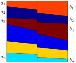
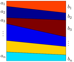
where $\{D_{i}\}_{i=1}^{n}$ are open subsets of $D$, moreover $D_{i}\cap D_{j}=\varnothing,\forall i\neq j$ and $\cup_{i=1}^{n}\overline{D_{i}}=\overline{D}$. Choices of the $D_{i}$ will be specified for two different geometric models in what follows and we use these models throughout the paper for both our analysis and our numerical experiments. They are illustrated in Figure 1(a) and Figure 1(b). To completely specify the models we need to parameterize the geometry $\{D_{i}\}_{i=1}^{n}$, and then describe the variability of the permeability within each subdomain $D_{i}.$ We now describe how these are both done.

(a) Layer Model with Fault

(b) Channelized Model

(c) Layer Model

Figure 1: Test Models

2.2.1 Geometric Parameterization

In the layer model of Figure 1(a), we assume that the interfaces between the layers are straight lines. The slope of the interface is determined by the thickness of each layer on the two sides. Hence, we use the layer thicknesses on the two sides to parameterize the geometry of the piecewise permeability function $\kappa(x)$. Furthermore, to describe potential faults, we introduce an additional parameter which determines the displacement of a vertical fault, whose horizontal location is specified. In the channel model, shown in Figure 1(b), we simply assume the channel to be sinusoidal as in [24]; the geometry can then be parameterized by the amplitude, frequency and width together with parameters defining the intersection of the channel with the boundaries. All of these models are then parameterized by a finite set of real numbers as we now detail, assuming that $D=(0,1)^{2}$ and letting $(x,y)\in D$ denote the horizontal and vertical respectively.

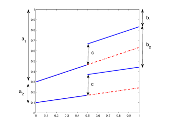
• Test Model $1$ (Layer Model with Fault): Given a fixed number $n$ of layers, the geometry in Figure 1(a) is determined by $\{a_{i}\}_{i=0}^{n}$ and $\{b_{i}\}_{i=0}^{n}$ and the slip $c$ that describes the (signed) height of the vertical fault at a specified location (for simplicity fixed at $x=\frac{1}{2}$). The geometry for the case of three layers is displayed in Figure 2(a). All the layers on the left hand side slip down$(c>0)$ or up $(c<0)$ with the same displacement $c$. Moreover because of the constraint that the layer widths are positive and sum to one we can reduce to finding the $2n-1$ parameters $a=(a_{1},\cdots,a_{n-1})$, $b=(b_{1},\cdots,b_{n-1})$, each in

  $$A:=\{\textbf{x}\in\mathbb{R}^{n-1}|\sum_{i=1}^{n-1}x_{i}\leq 1,x_{i}\geq 0\}\subset\mathbb{R}^{n-1},$$

  and $c\in C:=[-c^{\star},c^{\star}]$. For this case we then define the geometric parameter $u_{g}$ and the space of geometric parameters $U_{g}$ by

  $$u_{g}=(a,b,c),\qquad U_{g}=A^{2}\times C$$

  This geometric model thus has $2n-1$ parameters and $n$ domains $D_{i}$. Note that a particular case of this model is the layered model shown in Figure 1(c) where we take $c=0$ as a known parameter.

  

  (a) Two-layer configuration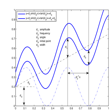

  

  (b) Channel configuration

  Figure 2: Geometry of Test Models

• Test Model $2$ (Channelized Model): Test model $2$ is shown in Figure 2(b). We assume that the lower boundary of the channel is described by the sinusoid

  $$y=d_{1}\sin(d_{2}x)+\tan(d_{3})x+d_{4}$$

  and we employ width parameter $d_{5}$. In this case, we characterize the geometric with

  $$u_{g}=(d_{1},\cdots,d_{5})\in\mathbb{R}^{5},\qquad U_{g}=\prod_{i=1}^{5}[{d_{i}^{-}},d_{i}^{+}].$$

  This geometric model thus has $5$ parameters and two domains $D_{1}$ and $D_{2}$ denoting the interior and exterior of the channel respectively, which gives $n=2$; note that $D_{2}$ contains disjoint components.

We now introduce an hypothesis that will be useful when we discuss the continuity of the forward map. Let $u_{g}^{\varepsilon}$ represent perturbations of $u_{g}$ and let the $D_{i}^{\varepsilon}$ be the corresponding induced perturbations of the domains $D_{i}$. Thus $\{D_{i}^{\varepsilon}\}_{i=1}^{n}$ is also a set of open subsets of $D$ such that $D_{i}^{\varepsilon}\cap D_{j}^{\varepsilon}=\varnothing$, for all $i\neq j$ and $\cup_{i=1}^{n}\overline{D_{i}^{\varepsilon}}=\overline{D}$.

Hypothesis 2.1.

For all $i\neq j$, the Lebesgue measure of $D_{j}^{\varepsilon}\cap D_{i}$, denoted as $|D_{j}^{\varepsilon}\cap D_{i}|$ goes to zero, if $u_{g}^{\varepsilon}\to u_{g}$.

It is clear that this hypothesis holds true for all the test models.

2.2.2 Permeability Values

Throughout the paper, we use $u_{\kappa}$ to denote the unknown parameters describing $\kappa_{i}$ in (4) and $U_{\kappa}$ as the admissible set for the parameters. We will consider two parameterizations of the functions $\kappa_{i}$ appearing in (4): as constants and as continuous functions.

• Piecewise constant: Each $\kappa_{i}$ is a positive constant. We then have the following choices:

  $$u_{\kappa}=(\kappa_{1},\cdots,\kappa_{n}),\qquad U_{\kappa}=(0,\infty)^{n}$$

• Continuous: We consider each $\kappa_{i}$ to be defined on the whole of $D$. We work with $\log\kappa$ as the exponential of this will always give a positive continuous function as required for the existence of solution to (1). This induces the following choices for $u_{\kappa}$ and $U_{\kappa}$:

  $$u_{\kappa}=(\log\kappa_{1},\dots,\log\kappa_{n}),\qquad U_{\kappa}=C({\overline{D}};\mathbb{R}^{n})$$

We may consider Test Models $1$ or $2$ with either constant or continuous $\kappa_{i}$, leading to four different models of the permeability. In all four cases we define the unknown parameter and associated space by

$$u=(u_{g},u_{\kappa}),\qquad U=U_{g}\times U_{\kappa}.$$

For the cases of defined above, $U$ is a subset of a separable Banach space $\bigl{(}\mathcal{B},\|\cdot\|_{{\mathcal{B}}}\bigr{)}$.

2.3 Observation Model

Given the parameterizations described at the end of the previous section, we define the function $F:U\rightarrow X$ as an abstract map from parameter space to the space of the permeabilities, by

$$F(u)=\kappa.$$ (5)

Let $L$ denote a bounded linear observation operator on $V$, comprising a finite number of linear functionals $l_{j}\in V^{*},j=1,\cdots,J$ that $L(p)=(l_{1}(p),\cdots,l_{J}(p))^{T}$. The measurements are some noisy observations from

$$y_{j}=l_{j}(p)+\eta_{j},$$

where $\eta_{j}$ represents the noise polluting the observation.

Let $y:=(y_{1},\cdots,y_{J})^{T}\in Y,$ where $Y:=\mathbb{R}^{J}$, equipped with Euclidean norm $|\cdot|$ and similarly for $\eta$; then, given (3,5), we define the observation operator $\mathcal{G}:U\rightarrow Y$ by $\mathcal{G}=L\circ G\circ F$. We then have

$$y=\mathcal{G}(u)+\eta.$$ (6)

In remaining sections of the paper we study the inverse problem of using $y$ to determine the unknown parameter $u\in U$. A key foundational result underlying our analysis is the the continuity of $\mathcal{G}$.

Theorem 2.2.

For all four of the permeability parameterizations the mapping $\mathcal{G}:U\subset\mathcal{B}\to Y$ is continuous.

Proof.

See the Appendix. ∎

3 Bayesian Inverse Problems

The inverse problem of interest here is to estimate the parameter $u$ from $y$ given by (6). We adopt a Bayesian approach. The pair $(u,y)\in\mathcal{B}\times\mathbb{R}^{J}$ is modeled as a random variable: we put a prior probability measure $\mu_{0}$ for $u$ viewed as an element of the separable Banach space $\mathcal{B}$, and define the random variable $y|u$ by assuming that $\eta\sim N(0,\Gamma)$ independently of $u$. The Bayesian solution to the inverse problem is then the posterior measure $\mu^{y}$ on the random variable $u|y.$ We thereby define the probabilistic information about the unknown $u$ in terms of the measurements $y$, forward model and prior information. The paper [39] and lecture notes [38] describe a mathematical framework for Bayes’ Theorem in this infinite dimensional setting. We define the priors and likelihood and then use this mathematical framework to establish the existence and well-posedness of the posterior distribution; here well-posedness refers to continuity of the posterior measure $\mu^{y}$, in the Hellinger or total variation metrics, with respect to the data $y$.

3.1 Prior Modeling

The unknown parameter $u$ is viewed as an element of the separable Banach space $\mathcal{B}$ defined for each of the four permeability models. Under the prior we assume that the physical parameter $u_{\kappa}$ is independent of the geometric parameter $u_{g}$. Therefore we can build up a prior measure $\mu_{0}$ by defining the geometric prior distribution density $\pi^{G}_{0}$ and the permeability (or log permeability) prior measure $\mu_{0}^{i}$ respectively.

3.1.1 Geometric Prior

In the layer model with a fault, the geometry variables $a,b$ satisfy the geometric constraint $a,b\in A$. In addition, we consider the case where there is no preference that the thickness of a certain layer is larger than another one. In other words, we consider the case where $a$ and $b$ are i.i.d random vector drawn from uniform distribution with a density $\pi_{0}^{A,g}(x)$ such that

$$\pi_{0}^{A,g}(x)=\left\{\begin{array}[]{cc}\frac{1}{|A|}&x\in A,\\ 0&x\notin A.\end{array}\right.$$ (7)

In addition, the slip parameter $c$ is drawn uniformly from $C=[-c^{\star},c^{\star}]$, and independently of $(a,b)$. Then, the prior density for this geometric model is

$$\pi_{0}^{G}(u_{g})=\pi_{0}^{A,g}(a)\pi_{0}^{A,g}(b)\pi_{0}^{C,g}(c)$$

For the Channel Model we assume the geometric parameter $u_{g}$ is drawn uniformly from the admissible set $U_{g}$. Therefore, we consider the prior

$$\pi_{0}^{G}(u_{g})=\Pi_{i=1}^{5}\pi_{0}^{[d_{i}^{-},d_{i}^{+}]}(d_{i})$$

3.1.2 Permeability Prior

We first discuss the case where the $\kappa_{i}$ are constant. Under the prior we assume that they are all independent and that each component $\kappa_{i}$ is drawn from a measure $\mu_{0}^{i}$ with Lebesgue density $\pi_{0}^{i}$, $i=1,\cdots,n$, defined by one of the following three cases:

• Lognormal: $\log\kappa_{i}$ has the Gaussian distribution $N(m_{i},\sigma_{i}^{2})$.

• Uniform: $\kappa_{i}$ has the uniform distribution in $[\kappa^{i,-},\kappa^{i,+}]$, where $\kappa^{i,-}>0$.

• Exponential: $\kappa_{i}$ has the exponential distribution with parameter $\lambda_{i}$.

In the case of variable $\kappa_{i}$ we will assume that each $\log\kappa_{i}$ is independent of the others and is distributed according to a random field prior $\mu_{0}^{i}=N(m_{i},C_{i})$ where the mean and covariance are chosen so that $\mu_{0}^{i}\Bigl{(}C({\overline{D}};\mathbb{R})\Bigr{)}=1$; that is, so that draws from $\mu_{0}^{i}$ give rise to continuous functions almost surely.

3.1.3 The Prior

Combining the foregoing we obtain, in the case of piecewise constant permeabilities, the following Lebesgue density of the prior for the Layer Model with fault:

$$\pi_{0}(u)=\pi_{0}^{A,g}(a)\pi_{0}^{A,g}(b)\pi_{0}^{C,g}(c)\prod_{i=1}^{n}\pi_{0}^{i}(\kappa_{i}).$$ (8)

This may be viewed as the Lebesgue density of a probability measure $\mu_{0}$ on $U$; here $U$ is finite dimensional. In the piecewise function case we have a prior measure $\mu_{0}$ on the infinite dimensional space $U$ and it is given by

$$\mu_{0}(du)=\pi_{0}^{A,g}(a)da\otimes\pi_{0}^{A,g}(b)db\otimes\pi_{0}^{C,g}(c)dc\otimes\prod_{i=1}^{n}\mu_{0}^{i}(d\alpha_{i}),$$ (9)

where $\alpha_{i}=\log\kappa_{i}.$ Thus in both cases we have constructed a measure $\mu_{0}$ in the measure space $\mathcal{B}$ equipped with the Borel $\sigma-$algebra. Furthermore the measure is constructed so that $\mu_{0}(U)=1.$ By similar arguments, we may construct the prior measure for the Channelized Models with the same properties. We omit the details for brevity.

3.2 Likelihood

We assume the noise $\eta$ in (6) is independent of $u$, and drawn from the Gaussian distribution $N(0,\Gamma)$ on $Y$, with $\Gamma$ a self-adjoint positive matrix. Thus $y|u\sim N(\mathcal{G}(u),\Gamma)$. We define the model-data misfit function $\Phi(u;y):U\times Y\rightarrow\mathbb{R}$ by

$$\Phi(u;y)=\frac{1}{2}|y-\mathcal{G}(u)|^{2}_{\Gamma},$$ (10)

where $|\cdot|_{\Gamma}=|\Gamma^{-\frac{1}{2}}\cdot|$. The negative log likelihood is given, up to a constant independent of $(u,y)$, by $\Phi(u;y).$

3.3 Posterior Distribution

We now show that the posterior distribution is well-defined by applying the basic theory in [39, 38]. Let $\mathbb{Q}_{0}$ be the Gaussian distribution $N(0,\Gamma)$. Define $\nu_{0}$ as a probability measure on $U\times Y$ by

$$\nu_{0}(du,dy)=\mu_{0}(du)\otimes\mathbb{Q}_{0}(dy).$$

The following Proposition 3.1 is a infinite dimensional version of Bayes Theorem, which implies the existence of a posterior distribution.

Proposition 3.1 (Bayes Theorem [38]).

Assume that $\Phi:U\times Y\rightarrow$ is $\nu_{0}$ measurable and that, for $y~{}\mathbb{Q}_{0}$ -a.s.,

$$Z=\int_{U}\exp(-\Phi(u;y))\mu_{0}(du)>0.$$

Then the conditional distribution of $u|y$ exists and is denoted $\mu^{y}$. Furthermore $\mu^{y}\ll\mu_{0}$ and for $y~{}\mathbb{Q}_{0}$ -a.s.,

$$\frac{d\mu^{y}}{d\mu_{0}}=\frac{1}{Z}\exp\left(-\Phi(u;y)\right).$$

We establish this Bayes theorem for our specific problem to show the well-definedness of the posterior distribution $\mu^{y}$. The key ingredient is the continuity of the forward and observation map $\mathcal{G}(u)$ (and hence $\Phi(\cdot;y)$) on a full $\mu_{0}$ measure set $U$; this may be used to establish the required measurability. We state two theorems, one concerning the case of piecewise constant permeability and the other concerning the case of variable permeability within each subdomain $D_{i}.$

Theorem 3.2 (Piecewise Constant).

Let $\Phi(u;y)$ be the model-data misfit function in (10), $\mu_{0}$ be the prior distribution in (8), then the posterior distribution $\mu^{y}$ is well-defined. Moreover, $\mu^{y}\ll\mu_{0}$ with a Radon-Nikodym derivative

$$\frac{d\mu^{y}}{d\mu_{0}}=\frac{1}{Z}\exp\left(-\Phi(u;y)\right),$$ (11)

where

$$Z=\int_{U}\exp(-\Phi(u;y))\mu_{0}(du)>0.$$

Proof.

Since $\mathcal{G}(u)$ is continuous on $U$ by Theorem 2.2, $\Phi(u;y)$ is continuous on $U\times Y$. We also have $\nu_{0}(U\times Y)=\mu_{0}(U)\mathbb{Q}_{0}(Y)=1$. Since $\Phi:U\times Y\to{\mathbb{R}}$ is continuous it is a measurable function (Borel) between the spaces $U\times Y$ and ${\mathbb{R}}$ equipped with their respective Borel $\sigma-$algebras. Note that, by using (2), we have

$$|\Phi(u;y)| =\frac{1}{2}|y-\mathcal{G}(u)|_{\Gamma}^{2}\leq|y|_{\Gamma}^{2}+|\mathcal{G}(u)|_{\Gamma}^{2}\leq|y|_{\Gamma}^{2}+\left(\frac{C}{\min\{\kappa_{i}\}}\right)^{2}.$$

Thus, for sufficiently small positive $\varepsilon>0$,

$$Z=\int_{U}\exp(-\Phi(u;y))\mu_{0}(du)\geq\int_{\cap_{i}\{\kappa_{i}>\varepsilon\}}\exp\left(-|y|_{\Gamma}^{2}-\left(\frac{C}{\varepsilon}\right)^{2}\right)\mu_{0}(du)$$

$$=\exp\left(-|y|_{\Gamma}^{2}-\left(\frac{C}{\varepsilon}\right)^{2}\right)\mu_{0}(\cap_{i}\{\kappa_{i}>\varepsilon\})=\exp\left(-|y|_{\Gamma}^{2}-\left(\frac{C}{\varepsilon}\right)^{2}\right)\Pi_{i=1}^{n}\mu_{0}^{i}(\{\kappa_{i}>\varepsilon\})>0.$$

Therefore, by Proposition 3.1 we obtain the desired result. ∎

Remark 3.3.

In the piecewise constant case $u$ is in a finite dimensional space. Then the posterior has a density $\pi^{y}$ with respect to Lebesgue measure and we can rewrite (11) as

$$\pi^{y}(u)=\frac{1}{Z}\exp(-\Phi(u;y))\pi_{0}(u),$$ (12)

which is exactly the usual Bayes rule.

Theorem 3.4 (Piecewise Continuous).

Let $\Phi(u;y)$ be the model-data misfit function in (10) and $\mu_{0}$ be the prior measure in (9), corresponding to Gaussian $\log\kappa_{i}$ in each domain. Then the posterior distribution $\mu^{y}$ is well-defined. Moreover, $\mu^{y}\ll\mu_{0}$ with a Radon-Nikodym derivative

$$\frac{d\mu^{y}}{d\mu_{0}}=\frac{1}{Z}\exp\left(-\Phi(u;y)\right),$$ (13)

where

$$Z=\int_{U}\exp(-\Phi(u;y))\mu_{0}(du)>0.$$

Proof.

Recall that the measure given by (9) is constructed so that $\mu_{0}(U)=1$. By the same argument as in the proof of Theorem 3.2, we deduce that $\Phi(u;y)$ is $\nu_{0}$ measurable. Again using (2), we have

$$|\Phi(u;y)|\leq|y|_{\Gamma}^{2}+\left(\frac{C}{\kappa_{\min}}\right)^{2},$$

where $\kappa_{\min}=\min\limits_{i,x}\kappa_{i}(x)$. Since $\kappa_{\min}\geq\min\limits_{i}\exp(-\|\alpha_{i}(x)\|_{\infty})$, we have

$$\frac{1}{\kappa_{\min}}\leq\max\limits_{i}\exp(\|\alpha_{i}(x)\|_{\infty})$$ (14)

Thus we have, using that Gaussian measure on a separable Banach space charges all balls with positive measure,

$$Z=\int_{U}\exp(-\Phi(u;y))\mu_{0}(du)\geq\int_{U}\exp\Bigl{(}-|y|_{\Gamma}^{2}-\left(\frac{C}{\kappa_{\min}}\right)^{2}\Bigr{)}\mu_{0}(du)$$

$$\geq\int_{\cap_{i}\{\|\alpha_{i}\|_{L^{\infty}}\leq 1\}}\exp\left(-|y|_{\Gamma}^{2}-C^{2}\max\limits_{i}\exp(2\|\alpha_{i}(x)\|_{\infty})\right)\mu_{0}(du)$$

$$\geq\int_{\cap_{i}\{\|\alpha_{i}\|_{L^{\infty}}\leq 1\}}\exp\left(-|y|_{\Gamma}^{2}-C^{2}\exp(2)\right)\mu_{0}(du)=\exp\left(-|y|_{\Gamma}^{2}-C^{2}\exp(2)\right)\mu_{0}(\cap_{i}\{\|\alpha_{i}\|_{L^{\infty}}\leq 1\})$$

$$=\exp\left(-|y|_{\Gamma}^{2}-C^{2}\exp(2)\right)\Pi_{i=1}^{n}\mu_{0}^{i}(\{\|\alpha_{i}\|_{L^{\infty}}\leq 1\})>0.$$

Thus we have the desired result. ∎

3.4 Well-Posedness

Now we study the continuity property of the posterior measure $\mu^{y}$ with respect to $y$. We recall definitions of the total variation metric $d_{TV}$ and Hellinger metric $d_{Hell}$ on measures, and then study Lipschitz and Hölder continuity of the posterior measure $\mu^{y}$, with respect to the data $y$, in these metrics.

Let $\mu$ and $\mu^{\prime}$ be two measures, and choose a common reference measure with respect to which both are absolutely continuous (the average of the two measures for example). Then the Hellinger distance is defined by

$$d_{{Hell}}(\mu,\mu^{\prime})=\left(\frac{1}{2}\int_{U}\left(\sqrt{\frac{d\mu}{d\nu}}-\sqrt{\frac{d\mu^{\prime}}{d\nu}}\right)^{2}d\nu\right)^{\frac{1}{2}}$$

and the Total variation distance $d_{TV}$ is defined by

$$d_{{TV}}(\mu,\mu^{\prime})=\frac{1}{2}\int_{U}\left|\frac{d\mu}{d\nu}-\frac{d\mu^{\prime}}{d\nu}\right|d\nu.$$

Furthermore, the Hellinger and total variation distance are related as follows:

$$\frac{1}{\sqrt{2}}d_{TV}(\mu,\mu^{\prime})\leq d_{{Hell}}(\mu,\mu^{\prime})\leq d_{{TV}}(\mu,\mu^{\prime})^{\frac{1}{2}}.$$ (15)

The Hellinger metric is stronger than total variation as, for square integrable functions, the Hellinger metric defines the right order of magnitude of perturbations to expectations caused by perturbation of the measure; the total variation metric does this only for bounded functions. See, for example, [39], section 6.7.

The nature of the continuity result that we can prove depends, in general, on the metric used and on the assumptions made about the prior model that we use for the permeability $\kappa$. This is illustrated for piecewise constant priors in the following theorem.

Theorem 3.5 (Piecewise Constant).

Assume that $\kappa(x)$ is a piecewise constant function correspond to parameter $u\in U\subset\mathcal{B}$. Let $\mu_{0}$ be a prior distribution on $u$ satisfying $\mu_{0}(U)=1$. The resulting posterior distribution $\mu(\textrm{resp.}~{}\mu^{\prime})\ll\mu_{0}$ with Radon-Nikodym derivative is given by (11), for each $y(\textrm{resp.}~{}y^{\prime})\in Y$. Then, for each of the test models we have:

1. for lognormal and uniform priors on the permeabilities, then for every fixed $r>0$, there is a $C_{i}=C_{i}(r),i=1,2$, such that, for all $y,y^{\prime}$ with $\max\{|y|_{\Gamma},|y^{\prime}|_{\Gamma}\}<r$,

   $$d_{{TV}}(\mu,\mu^{\prime})\leq C_{1}\left|y-y^{\prime}\right|_{\Gamma},$$

   $$d_{{Hell}}(\mu,\mu^{\prime})\leq C_{2}\left|y-y^{\prime}\right|_{\Gamma};$$

2. for exponential priors on the permeabilities, then for every fixed $r>0$ and $\iota\in(0,1)$ there is $K_{i}=K_{i}(r,\iota)$ such that for all $y,y^{\prime}$,with $\max\{|y|_{\Gamma},|y^{\prime}|_{\Gamma}\}<r$,

   $$d_{{TV}}(\mu,\mu^{\prime})\leq K_{1}\left|y-y^{\prime}\right|_{\Gamma}^{\iota},$$ (16)

   $$d_{{Hell}}(\mu,\mu^{\prime})\leq K_{2}\left|y-y^{\prime}\right|_{\Gamma}^{\frac{\iota}{2}}.$$ (17)

Remark 3.6.

For (ii), we only need to prove (16), since (17) then follows from (15). We can also deduce (17) directly by a similar argument as the proof of (16), but this does not improve the Hölder exponent. Mathematically it would be possible to use uniform priors on the permeabilities whose support extends to include the origin; in terms of well-posedness this would result in a degradation of the Hölder exponent as we see in Theorem 3.5(ii) for exponential priors.

Proof.

First note that

$$|\Phi(u;y)-\Phi(u,y^{\prime})|=\left|\frac{1}{2}|y-\mathcal{G}(u)|_{\Gamma}^{2}-\frac{1}{2}|y^{\prime}-\mathcal{G}(u)|_{\Gamma}^{2}\right|=\frac{1}{2}\left|\langle y-y^{\prime},y+y^{\prime}-2\mathcal{G}(u)\rangle_{\Gamma}\right|$$

$$\leq\left(r+|\mathcal{G}(u)|_{\Gamma}\right)|y-y^{\prime}|_{\Gamma}.$$ (18)

We denote the Lipschitz constant

$$M(r,u):=r+|\mathcal{G}(u)|_{\Gamma}.$$

Throughout the rest of this proof, the constant $C$ may depend on $r$ and changes from occurrence to occurrence. Let $Z$ and $Z^{\prime}$ denote the normalization constant for $\mu^{y}$ and $\mu^{y^{\prime}}$, so that

$$Z=\int_{U}\exp(-\Phi(u;y))\mu_{0}(du)\qquad\textrm{and}\qquad Z^{\prime}=\int_{U}\exp(-\Phi(u;y^{\prime}))\mu_{0}(du).$$

By (2) $Z$ has a positive lower bound as we now show:

$$Z\geq\int_{\cap_{i}\{\kappa_{i}>\varepsilon\}}\exp\left(-|y|_{\Gamma}^{2}-\left(\frac{C}{\varepsilon}\right)^{2}\right)\mu_{0}(du)\geq\exp\left(-r^{2}-\left(\frac{C}{\varepsilon}\right)^{2}\right)\mu_{0}(\cap_{i}\{\kappa_{i}>\varepsilon\})>0,$$

when $|y|_{\Gamma}<r$ and $\varepsilon>0$, which should be sufficiently small in the case of uniform prior. We have an analogous lower bound for $Z^{\prime}$.

The proof of (i) is an application of Theorem 4.3 in [38]: if the prior measure for $\kappa$ is uniform distribution with $\kappa_{min}>0$, or a lognormal distribution, then $M^{2}(r,u)\in L^{1}_{\mu_{0}}$, which leads to Lipschitz continuity.

Proof of (ii): We just need to prove (16). If we substitute $\mu$ and $\mu^{\prime}$ into $d_{TV}(\mu,\mu^{\prime})$, we have

$$d_{{TV}}(\mu,\mu^{\prime})\leq I_{1}+I_{2}.$$

where

$$I_{1}=\frac{1}{2Z}\int_{U}\left|\exp\left(-\Phi(u,y)\right)-\exp\left(-\Phi(u,y^{\prime})\right)\right|d\mu_{0}$$

$$I_{2}=\frac{1}{2}|Z^{-1}-(Z^{\prime})^{-1}|\int_{U}\exp\left(-\Phi(u,y^{\prime})\right)d\mu_{0}.$$

Note that

$$|Z^{-1}-(Z^{\prime})^{-1}| =\frac{|Z-Z^{\prime}|}{ZZ^{\prime}}\leq\frac{1}{ZZ^{\prime}}\int_{U}\left|\exp\left(-\Phi(u,y)\right)-\exp\left(-\Phi(u,y^{\prime})\right)\right|d\mu_{0}=\frac{2}{Z^{\prime}}I_{1}.$$

Thus, by using the positive bound on $Z^{\prime}$ from below, we have

$$I_{2}\leq CI_{1}.$$

Therefore, we just need to estimate $I_{1}$. For any $\iota\in(0,1)$,

$$2ZI_{1}=\int_{U}\left|\exp\left(-\Phi(u,y)\right)-\exp\left(-\Phi(u,y^{\prime})\right)\right|\mu_{0}(du)$$

$$=\int_{\{|\Phi(u,y)-\Phi(u,y^{\prime})|\leq 1\}}|\exp\left(-\Phi(u,y)\right)-\exp\left(-\Phi(u,y^{\prime})\right)|\mu_{0}(du)$$

$$+\int_{\{|\Phi(u,y)-\Phi(u,y^{\prime})|>1\}}|\exp\left(-\Phi(u,y)\right)-\exp\left(-\Phi(u,y^{\prime})\right)|\mu_{0}(du)$$

$$\leq\int_{\{|\Phi(u,y)-\Phi(u,y^{\prime})|\leq 1\}}|\Phi(u,y)-\Phi(u,y^{\prime})|^{\iota}\mu_{0}(du)+2\mu_{0}\left(\{|\Phi(u,y)-\Phi(u,y^{\prime})|>1\}\right).$$

By (32) and Lemma 7.2, we have

$$2ZI_{1}\leq\int_{U}M^{\iota}(r,u)d\mu_{0}~{}|y-y^{\prime}|_{\Gamma}^{\iota}+2\int_{U}M^{\iota}(r,u)d\mu_{0}~{}|y-y^{\prime}|_{\Gamma}^{\iota}=3\int_{U}M^{\iota}(r,u)d\mu_{0}~{}|y-y^{\prime}|_{\Gamma}^{\iota}.$$

By using the positive lower bound on $Z$, for any $\iota\in(0,1)$, we have

$$I_{1}\leq C_{1}|y-y^{\prime}|_{\Gamma}^{\iota}$$

Thus

$$d_{{TV}}(\mu,\mu^{\prime})\leq I_{1}+I_{2}\leqslant C_{1}\left|y-y^{\prime}\right|_{\Gamma}^{\iota}+C_{2}\left|y-y^{\prime}\right|_{\Gamma}^{\iota}\leqslant K_{1}(r)\left|y-y^{\prime}\right|_{\Gamma}^{\iota}$$

therefore, we obtain

$$d_{{TV}}(\mu,\mu^{\prime})\leq K_{1}\left|y-y^{\prime}\right|_{\Gamma}^{\iota},\quad 0<\iota<1,$$

which completes the proof. ∎

As for the piecewise function case, we have a similar well-posedness result, which shows Lipschitz continuity with respect to data.

Theorem 3.7 (Piecewise Continuous).

Assume that $\kappa(x)$ is a piecewise continuous function corresponding to parameter $u\in U\subset\mathcal{B}$ and that the prior $\mu_{0}$ is Gaussian on the variable $\log\kappa_{i}$ and satisfies $\mu_{0}(U)=1.$ The resulting posterior distribution is $\mu(resp.~{}\mu^{\prime})\ll\mu_{0}$ with Radon-Nikodym derivative given by (13), for each $y(resp.~{}y^{\prime})\in Y$. Then, for each of the test models we have that for every fixed $r>0$, there is a $C_{i}=C_{i}(r),i=1,2$, such that, for all $y,y^{\prime}$ with $\max\{|y|_{\Gamma},|y^{\prime}|_{\Gamma}\}<r$,

$$d_{{TV}}(\mu,\mu^{\prime})\leq C_{1}\left|y-y^{\prime}\right|_{\Gamma},\qquad d_{{Hell}}(\mu,\mu^{\prime})\leq C_{2}\left|y-y^{\prime}\right|_{\Gamma}.$$

Proof.

We just need to prove the Hellinger distance case as the TV distance case then follows from (15). The remainder of the proof is an application of the methods used Theorem 4.3 in [38] with $M_{1}=0$ and

$$M_{2}=r+C\max_{i}\exp(\|\alpha_{i}(x)\|_{\infty}),$$

after noting that the normalization constant $Z>0.$ By (14), we obtain

$$\int_{U}M_{2}^{2}d\mu_{0} \leq 2r^{2}\mu_{0}(U)+2C^{2}\int_{U}\max_{i}\exp(2\|\alpha_{i}(x)\|_{\infty})d\mu_{0}$$

$$\leq 2r^{2}\mu_{0}(U)+2C^{2}\sum_{i=1}^{n}\int_{U}\exp(2\|\alpha_{i}(x)\|_{\infty})d\mu_{0}$$

Since for any $\epsilon>0$, there exist a $C(\epsilon)$ that $\exp(x)\leq C(\epsilon)\exp(\epsilon x^{2})$ we obtain that for each $i$,

$$\int_{U}\exp(2\|\alpha_{i}(x)\|_{\infty})d\mu_{0}\leq C(\epsilon)\int_{U}\exp(\epsilon\|\alpha_{i}(x)\|^{2}_{\infty})d\mu_{0}.$$

From the Fernique Theorem we deduce that, as long as $\epsilon$ is small enough,

$$\int_{U}M^{2}(r,u)d\mu_{0}<\infty.$$

∎

4 MCMC Algorithm

We have demonstrated the existence and well-posedness of the posterior distribution, which is the Bayesian solution to the inverse problem (6). We now demonstrate numerical methods to extract information from this posterior distribution; one way to do this, which we focus on in this paper, is to generate samples distributed according to the posterior distribution. These can be used to approximate expectations with respect to the posterior and hence to make predictions about, and quantify uncertainty in, the permeability. In this section we construct a class of MCMC methods to generate such samples, using a Gibbs splitting to separate geometric and physical parameters, and using Metropolis (within Gibbs) proposals which exploit the structure of the prior. We thereby generate samples from the posterior given by (11) or (13) in Theorems 3.2 and 3.4, respectively. The resulting accept-reject parts of the algorithm depend only on differences in the log-likelihood at the current and proposed states, or alternatively on differences of the misfit function $\Phi$ given by (10). Similar methods have been identified as beneficial for Gaussian priors in [35, 8] for example and here we extend to the non-Gaussian prior measure on the permeability values (uniform distribution and exponential distribution) and on the geometry.

4.1 Prior Reversible Proposals

We start by demonstrating how prior reversible proposals lead to a simple accept-reject mechanism, depending only on differences in the model-data misfit function, within the context of the Metropolis-Hasting algorithm applied to Bayesian inverse problems. When the target distribution has density $\pi$ defined on $\mathbb{R}^{d}$ this algorithm proceeds by proposing to move from current state $u$ to proposed state $v$, drawn from Markov kernel $q(u,v)$, and accepting the move with probability

$$a(u,v)=\frac{\pi(v)q(v,u)}{\pi(u)q(u,v)}\wedge 1.$$ (19)

Crucial to this algorithm is the design of the proposal $q(u,v)$; algorithm efficiency will increase if we use a proposal which leads to low integrated correlation in the resulting Markov chain.

When we have piecewise constant permeabilities then the posterior density $\pi^{y}$ is given by (12) with $\Phi$ defined in (10). If we chose a prior-reversible proposal density which then satisfies

$$\pi_{0}(u)q(u,v)=\pi_{0}(v)q(v,u)\quad u,v\in\mathbb{R}^{d}.$$ (20)

then the acceptance probability from (19) becomes

$$a(u,v) =\frac{\pi^{y}(v)q(v,u)}{\pi^{y}(u)q(u,v)}\wedge 1=\frac{\pi_{0}(v)\exp(-\Phi(v;y))q(v,u)}{\pi_{0}(u)\exp(-\Phi(u;y))q(u,v)}\wedge 1$$

so that

$$a(u,v)=\exp(\Phi(u;y)-\Phi(v;y))\wedge 1.$$ (21)

Thus, if the proposed state $v$ corresponds to a lower value of the model-data misfit function $\Phi(v;y)$ than the current state $\Phi(u;y)$, it will accept the proposal definitely, otherwise it will accept with probability $a(u,v)<1.$ Hence, the accept-reject expressions depend purely on the model-data mismatch function $\Phi(u;y)$, having clear physical interpretation.

4.2 Prior Reversible Proposal on $\mathbb{R}^{d}$

We now construct prior reversible proposals for the finite dimensional case when the permeability is piecewise constant. In this case $u_{\kappa}$ lives in a subset $U$ of $\mathbb{R}^{n}$ where $n$ is the number of parameters to be determined. The prior distribution $\pi_{0}$ constrains the parameters to the admissible set $U$, that is $\pi_{0}(x)=0$ if $x\notin U$. Given current state $v$ we then construct a prior reversible proposal kernel $q$ as follows: we let

$$v=\left\{\begin{array}[]{ll}w&w\in U\\ u&w\notin U\end{array}\right.,$$ (22)

where $w$ is drawn from kernel $p(u,w)$ that satisfies

$$\pi_{0}(u)p(u,w)=\pi_{0}(w)p(w,u)\quad\forall u,w\in U.$$ (23)

Note that the previous expression is constrained to $U$, rather than $\mathbb{R}^{d}$ as in (20). Note, however, that we have not assumed that $p(u,v)$ is a Markov kernel on $U\times U$; it may generate draws outside $U$. Therefore, in (22) we just simply accept or reject the proposal $w$ based on whether $w$ is in $U$ or not. The reversibility with respect to the prior of the proposal $q(u,v)$ given by (22) follows from:

Proposition 4.1.

Consider the Markov kernel $q(u,v)$ on $U\times U$ defined via (22)-(23). Then

$$\pi_{0}(u)q(u,v)=\pi_{0}(v)q(v,u)\quad\forall u,v\in U.$$

Proof.

See Appendix. ∎

For a uniform prior $\pi_{0}(u)$, $p(u,w)$ may be any symmetric function that satisfies $p(u,w)=p(w,u)$. For example, we can use a Gaussian local move such that $p(u,w)\propto\exp\left(-\frac{1}{2\varepsilon^{2}}|w-u|^{2}\right)$ or we can also propose $w$ by a local move drawn uniformly from an $\epsilon$ ball around $u$. An analogous discussion also applies when the geometric parameter is uniform (as before) but the permeability values are exponential. For the exponential permeability prior $\exp(\lambda)$, with support $[0,\infty)$, we may choose $w=u-\lambda\delta+\sqrt{2\delta}\xi$ with $\xi\sim\mathcal{N}(0,1)$. For all these examples, it is easy to check that the proposal density $p(u,w)$ satisfies (23). Therefore, by Proposition 4.1 we obtain that the proposal (22) is reversible with respect to the prior. Thus, the acceptance probability that results is given by (21).

4.3 Prior Reversible Proposal on $C({\overline{D}};\mathbb{R}^{n})$

For the case of continuous permeabilities, we recall that $u_{\kappa,i}=\log\kappa_{i}$ has prior Gaussian measure $\mu_{0}^{\kappa}(du_{\kappa})=\mathcal{N}(m,C)$ with covariance and mean chosen so that it charges the space $C({\overline{D}};\mathbb{R}^{n})$ with full measure. In this case a prior reversible proposal is given by

$$v_{\kappa}=m+\sqrt{1-\beta^{2}}(u_{\kappa}-m)+\beta\xi,\quad\xi\sim\mathcal{N}(0,C),~{}\beta\in[0,1].$$

This is the pCN-MCMC method introduced in [1] (see the overview in [8]) and the acceptance probability is again given by (21) in this infinite dimensional context.

4.4 Metropolis-within-Gibbs: Separating Geometric and Physical Parameters

In practice the geometric and physical parameters have very different effects on the model-data misfit and efficiency can be improved by changing them separately. Using the independence between the geometric parameter $u_{g}$ and the physical parameters (permeabilities) $u_{\kappa}$ this can be obtained by employing the following Metropolis-within-Gibbs algorithm.

Algorithm 4.2 (Metropolis-within-Gibbs).

Initialize $u^{(0)}=(u_{\kappa}^{(0)},u_{g}^{(0)})\in U$.
For $k=0,\dots$

1. Propose $v_{g}$ from $q_{g}(u_{g}^{(k)},v_{g})$

   (1.1) Draw $w\in\mathbb{R}^{d}$ from $p_{g}(u^{(k)}_{g},w)$.

   (1.2) Let $v_{g}\in U_{g}$ defined by

   $$v_{g}=\left\{\begin{array}[]{ll}w&w\in U\\ u_{g}^{(k)}&w\notin U\end{array}\right..$$

2. Accept or reject $v=(u_{\kappa}^{(k)},v_{g})$:

   $$(u_{\kappa}^{(k)},u_{g}^{(k+1)})=\left\{\begin{array}[]{cc}v&\mathrm{with~{}probability}~{}a(u^{(k)},v)\\ u^{(k)}&\mathrm{otherwise}\end{array}\right..$$

   where $u^{(k)}\equiv(u_{\kappa}^{(k)},u_{g}^{(k)})$ and with $a(u,v)$ defined by (21).

3. Propose $v_{\kappa}$ from $q_{\kappa}(u_{\kappa}^{(k)},v_{\kappa})$:
   In the constant permeabilities case, propose $v_{\kappa}$ from $q_{\kappa}(u_{\kappa}^{(k)},v_{\kappa})$ as follows

   (3.1) Draw $w\in\mathbb{R}^{d}$ from $p_{\kappa}(u_{\kappa}^{(k)},w)$.

   (3.2) Let $v_{\kappa}\in U_{\kappa}$ defined by

   $$v_{\kappa}=\left\{\begin{array}[]{ll}w&w\in U_{\kappa}\\ u_{\kappa}^{(k)}&w\notin U_{\kappa}\end{array}\right..$$

   In the continuous permeabilities case we propose $v_{\kappa}$ according to

   $$v_{\kappa}=m+\sqrt{1-\beta^{2}}(u_{\kappa}^{(k)}-m)+\beta\xi,\quad\xi\sim\mathcal{N}(0,C),~{}\beta\in[0,1],\\$$

4. Accept or reject $v=(v_{\kappa},u_{g}^{(k+1)})$:

   $$(u_{\kappa}^{(k+1)},u_{g}^{(k+1)})=\left\{\begin{array}[]{cc}v&\mathrm{with~{}probability}~{}a(\hat{u}^{(k)},v)\\ \hat{u}^{(k)}&\mathrm{otherwise}\end{array}\right..$$

   where $\hat{u}^{(k)}\equiv(u_{\kappa}^{(k)},u_{g}^{(k+1)})$ and with $a(u,v)$ defined by (21).

Furthermore, in the experiments which follow we sometimes find it advantageous to split the geometric parameters into different groupings, and apply the Metropolis-within-Gibbs idea to these separate groupings; again the independence of the parameters under the prior allows this to be done in a straightforward fashion, generalizing the preceding Algorithm 4.2. In particular, by using the independence of the geometric parameters under the prior, together with prior-reversibility of the proposals used, it again follows that the accept-reject criterion for each Metropolis-within-Gibbs step is given by (21). In addition, we generate multiple parallel MCMC chains to sample the posterior in the subsequent experiments. For some of those chains we often find that a low probability mode is explored for a very large number of iterations. In order to accelerate the convergence of these chains, within the Metropolis step of the aforementioned algorithm, we implement proposals where the local moves described earlier are replaced, with probability 1/2, by independent samples from the prior.

5 Numerical Experiments

We present some numerical examples to demonstrate the feasibility of our methodology. Specifically, the performance is illustrated by application to three examples derived from our Test Models of Section 2. For these examples, the forward model consists of the elliptic equation on a domain $D=[0,1]\times[0,1]$ discretized with the finite difference method on a mesh of size $50\times 50$. In addition, $J$ measurement functionals $\ell_{j}(p)$ are defined by

$$\ell_{j}(p)=\frac{1}{2\pi\sigma^{2}}\int_{D}\exp\left(-\frac{|x-x_{j}|^{2}}{2\sigma^{2}}\right)p(x)dx,\qquad j\in\{1,\cdots,J\}$$ (24)

which can be understood as a smooth approximation of pressure evaluations at certain locations $x_{j}$’s in the domain $D$. This is because the kernel under the integrand approaches a Dirac measure at $x_{j}$ as $\sigma\to 0.$ Note that $\ell_{j}\in V^{*}$, the dual space of $V$, as required for the analysis of Section 2. In all of the numerical experiments reported $\sigma$ takes the value $0.01.$

For the subsequent experiments we generate synthetic data by first computing $p^{\dagger}$, the solution to the elliptic equation with a “true” permeability $\kappa^{\dagger}(x)$ associated to the true parameters $u^{\dagger}$. Then, synthetic data is defined by $y_{j}=\ell_{j}(p^{\dagger})+\eta_{j}$, where $\eta_{j}$ are i.i.d. Gaussian noise from $\mathcal{N}(0,\gamma^{2})$. Our choices of $u^{\dagger}$ and $\gamma$ are described below. In order to avoid the inverse crime, the synthetic data is computed from the true permeability defined on a domain discretized on $100\times 100$ cells while the Bayesian inversions are performed on a $50\times 50$ grid. It is important to remark that the effect of the observational noise, at the scale we introduce it, is sufficient to induce significant inversion challenges even in this perfect model scenario. Furthermore, if model error is to be studied, it is perhaps more pertinent to study the effect of modelling the geometry through a small finite set of parameters, when real interfaces and faults will have more nuanced structures, or the effect of modelling spatially varying fields as constants. We leave the detailed study of these and other grid-based model errors for separate study.

5.1 Example. A Three-layer Model With Fault

For this experiment we consider a permeability of the form

$$\kappa(x)=\kappa_{1}\chi_{D_{1}}(x)+\kappa_{2}\chi_{D_{2}}(x)+\kappa_{3}\chi_{D_{3}}(x)$$ (25)

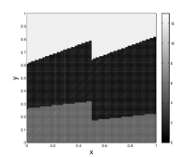
where $\{D_{i}\}_{i=1}^{3}$ are the open subsets defined by the geometric parameters $a=(a_{1},a_{2})$, $b=(b_{1},b_{2})$ and $c$ as in Figure 2(a). Therefore, the unknown parameter is $u=(a_{1},a_{2},b_{1},b_{2},c,\kappa_{1},\kappa_{2},\kappa_{3})\in\mathbb{R}^{8}$. We consider the true $\kappa^{\dagger}(x)$ shown in Figure 3 (top-left) which corresponds to (25) for the true values $u^{\dagger}$ of Table 1.

parameter	true value	data set 1	data set 1	data set 2	data set 2
		mean	variance	mean	variance
$a_{1}$	$0.39$	0.386	$3.4\times 10^{-3}$	0.394	$2\times 10^{-4}$
$b_{1}$	$0.18$	0.174	$4.6\times 10^{-3}$	0.177	$7\times 10^{-4}$
$a_{2}$	$0.35$	0.486	$6.9\times 10^{-3}$	0.400	$6\times 10^{-4}$
$b_{2}$	$0.6$	0.618	$8.9\times 10^{-3}$	0.637	$3.5\times 10^{-3}$
$c$	$0.15$	0.239	$1.04\times 10^{-2}$	0.192	$1.2\times 10^{-3}$
$\kappa_{1}$	$12$	11.718	1.796	11.337	$1.0128$
$\kappa_{2}$	$1$	1.228	$4.57\times 10^{-2}$	1.177	$9.5\times 10^{-3}$
$\kappa_{3}$	$5$	5.148	$6.65\times 10^{-1}$	4.55	$1.378\times 10^{-1}$

Table 1: Data relevant to the experiment with the 3-layers model

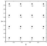
We consider 16 measurement functionals defined by (24) with measurement locations distributed as shown in Figure 3 (top-right). Synthetic data (data set 1) is generated as described above with $\gamma=2\times 10^{-3}$.

According to subsection 3.1, the prior distribution for this parameter is defined by

$$\pi_{0}(u)=\pi_{0}^{A,g}(a)\pi_{0}^{A,g}(b)\pi_{0}^{C,g}(c)\pi_{0}^{1}(\kappa_{1})\pi_{0}^{2}(\kappa_{2})\pi_{0}^{3}(\kappa_{3})$$

where each of the $\pi_{0}^{i}(\kappa_{i})$ and $\pi_{0}^{C,g}(c)$ is a uniform distribution on a specified interval. The uniform prior associated to the geometrical parameters $a$ and $b$ is defined with support everywhere on the edges of the squared domain. However, specific restricted intervals are specified for the construction of the uniform priors corresponding to the values of the permeabilities and, in particular, we choose intervals which do not include the origin. The reason for selecting these restrictive priors for the values of the permeabilities is motivated by the subsurface flow application where prior knowledge of a range of nominal values of permeabilities for each rock-type are typically available from geologic data. The densities $\pi_{0}^{A,G}(a)$ and $\pi_{0}^{A,G}(b)$ are defined according to expression (7) where $A=\{\textbf{x}\in\mathbb{R}|x_{1}+x_{2}\leq 1,x_{1}\geq 0,x_{2}\geq 0\}$. In the top row of Figure 4 we display some permeabilities defined by (25) for parameters $u$ drawn from the prior distribution defined by the previous expression.

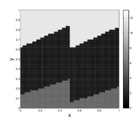
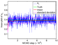
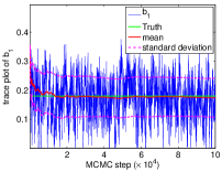
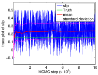
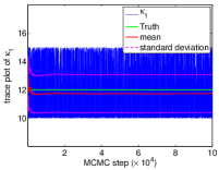
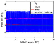
The forward model, the prior distribution and the synthetic data described above define the posterior measure given by (11), Theorem 3.2, that we sample with a variant of the MCMC method of Algorithm 4.2. In concrete, we implement the outer Gibbs loop by considering groupings of the unknown $u=(a_{1},a_{2},b_{1},b_{2},c,\kappa_{1},\kappa_{2},\kappa_{3})$ as follows: (i) the high permeabilities $\kappa_{1}$ and $\kappa_{3}$, (ii) the low permeability $\kappa_{2}$, (iii) the slip $c$, (iv) the right-hand lengths $a=(a_{1},a_{2})$ and (v) the left-hand lengths $b=(b_{1},b_{2})$. This separation of the unknown results in short decorrelation times compared to the ones when more variables of the unknown are updated simultaneously within the Metropolis part of Algorithm 4.2. We consider 20 different chains started with random draws from the prior. Trace plots from the first $10^{5}$ steps of one of the chains is presented in Figure 5, together with the running mean and standard deviations. We monitor the convergence of the multiple chains with the multivariate potential scale reduction factor (MPSRF) [2]. Once approximate convergence has been reached, all chains are merged and the samples from the combined chains are used for the subsequent results. In the middle row of Figure 4 we show permeabilities (defined by (25)) for some samples $u$ of the posterior distribution. In Table 1 we display the values of the mean $\hat{u}$ and the variance of the posterior measure characterized with a total of $1.5\times 10^{7}$ samples from our MCMC chains. The permeability that results from (25) for the mean parameter $\hat{u}$ of the posterior is presented in Figure 3 (bottom-left).

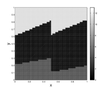
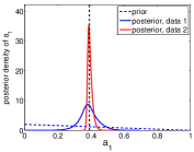
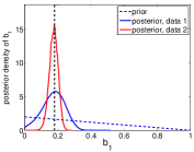
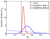
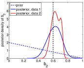
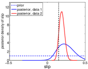
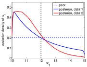
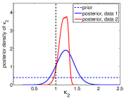
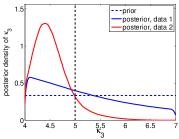
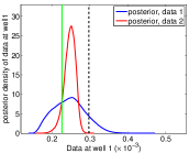
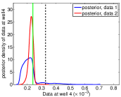
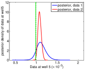
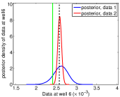
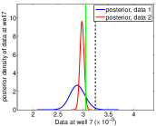
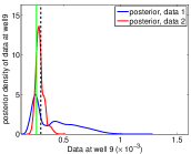
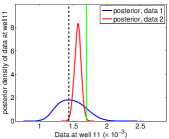
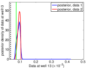
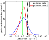
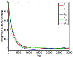
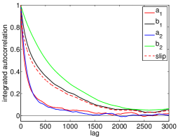
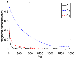
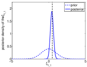
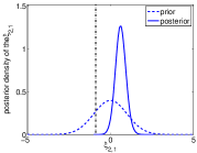
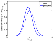
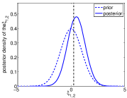
We now repeat this experiment with a different set of synthetic data (data set 2) generated as before but with a smaller error with standard deviation $\gamma=5\times 10^{-4}$. This set of synthetic data defines a new posterior measure that we characterize with the MCMC Algorithm 4.2 used for the previous experiments (using exactly the same parameters in the proposal generators). The corresponding values of $u$ are also displayed in Table 1 and the resulting permeability is displayed in Figure 3 (bottom-right). Some permeabilities associated to the samples of the posterior are presented in Figure 4 (bottom row ). For both experiments, the marginals of the posterior distribution are displayed in Figure 6 along with the marginals of the prior. The marginals of the posterior pushed forward by the forward operator are displayed in Figure 7. In Figure 8 we display the integrated autocorrelation for each of the components of the unknown for both posterior that arise from the data set 1 (top) and the data set 2 (bottom).

From Table 1 we observe that, for both experiments, the mean of the parameters are in very good agreement with the truth. In fact, the corresponding permeabilities from Figures 3 produce very similar results. However, it comes as no surprise that more accurate synthetic data (data set 2) result in a posterior density that is more peaked around the truth ( see Figure 6). In other words, the posterior associated with smaller error variance quantifies less uncertainty in the unknown parameters. While both estimates provide a good approximation of the truth, the associated uncertainties are substantially different from one another. Indeed, from Figure 4 we observe a larger variability in the samples of the posterior that we obtain from the data set 1.

From Figure 8 we note that the correlation of the samples is larger for observational error with smaller covariance. Indeed, during the MCMC algorithm for sampling of the posterior, the local move in the proposal is more likely to be rejected for smaller values of $\gamma$ (recall we are using the same MCMC algorithm for both experiments).

Figure 3: Permeabilities for the 3-layers fault model. Top-left: truth. Top-right: measurement locations. Bottom-left: mean (from less accurate data). Bottom-right: mean (from more accurate data).

Figure 4: Permeabilities defined by (25) from samples of the prior (top row), posterior with less accurate measurements (middle row) and posterior with more accurate measurements (bottom-row)

Figure 5: Trace plot from one MCMC chain (data set 1). Top: three geometric parameters. Bottom: permeability values

Figure 6: Prior and posterior densities of the unknown $u$. Vertical line indicates the true value of $u$.

Figure 7: Posterior densities of the data predictions $G(u)$. Vertical lines indicate the nominal value of synthetic observations: dotted black (less accurate), green (more accurate)

Figure 8: Autocorrelation from one MCMC chain. Top: data 1. Bottom: data 2. Left: geometric parameters. Right: permeability values.

5.2 Example. Two-layer Model With Spatially-varying Permeabilities

This is an infinite-dimensional example where the permeability is described by

$$\kappa(x)=\kappa_{1}(x)\chi_{D_{1}}(x)+\kappa_{2}(x)\chi_{D_{2}}(x)$$ (26)

where $D_{1}$ and $D_{2}$ are the subsets defined by $a$ and $b$ as shown in Figure 1(c). For this case we consider the case that $c=0$ is a known parameter. The unknown parameter in this case is $u=(a,b,\log\kappa_{1},\log\kappa_{2})\in[0,1]^{2}\times C({\overline{D}};\mathbb{R}^{2})$.

We consider a prior measure of the form

$$\mu_{0}(du)=\pi_{0}^{A,g}(a)da~{}\pi_{0}^{A,g}(b)db~{}\delta(c)\otimes N(m_{1},C_{1})N(m_{2},C_{2})$$ (27)

where $\delta$ is the Dirac distribution ($c=0$ is known) and where $A=[0,1]$ and $C_{1}$ and $C_{2}$ are covariance operators defined from correlation functions typical in geostatistics [37]. In concrete the correlation functions of $C_{1}$ (resp. $C_{2}$) is spherical (resp. exponential) and its maximum correlation is along $\pi/4$ (resp. $3\pi/4$) [37]. It is convenient, both conceptually and computationally, to parameterize the log permeabilities via their Karhunen-Loeve (KL) expansions of the form

$$\log(\kappa_{i}(x))=m_{i}+\sum_{j=1}^{\infty}\sqrt{\lambda_{j,i}}v_{j,i}(x)\xi_{j,i}$$ (28)

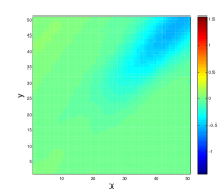
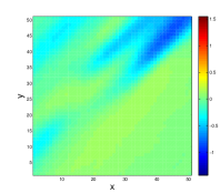
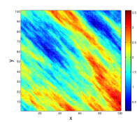
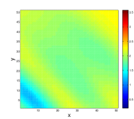
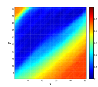
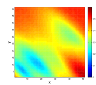
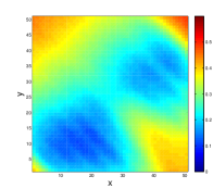
where $\lambda_{j,i}$ and $v_{j,i}(x)$ are the eigenvalues and eigenfunctions of $C_{i}$ and $\xi_{j,i}\in\mathbb{R}$. We assume that in the previous expression $\{\lambda_{j,i}\}_{j=1}^{\infty}$ are ordered as $\lambda_{1,i}\geq\lambda_{2,i}\geq\cdots$. Under this representation, $\xi_{j,i}\sim N(0,1)$ produces $\log\kappa_{i}\sim N(m_{i},C_{i})$. Thus, the KL representation enables us to sample from the prior distribution and therefore generate proposals in Algorithm 4.2. For the numerical implementation of the Bayesian inversion, we consider expression (28) truncated to $N=50^{2}$ terms corresponding to all the eigenvectors of the discretized (on a $50\times 50$ grid) covariance $C_{i}$. However we emphasize that the approach we adopt corresponds to a well-defined limiting Bayesian inverse problem in which the series is not truncated and the PDE is solved exactly. The theory of paper [6] may be used to quantify the error arising from the truncation of the KL expansion and the approximation of the solution of the PDE; this gives a distinct advantage to the “apply then discretize” approach advocated here since all sufficiently resolved computations are approximating the same limiting problem. In Figure 9 (top row) we show log-permeabilities computed with (26) with parameter $u$ sampled from the prior (27). There is substantial variability in these samples.

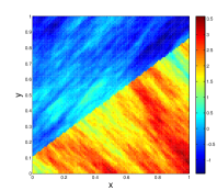
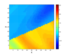
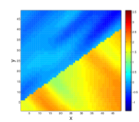
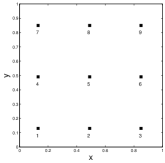
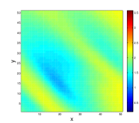
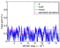
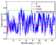
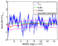
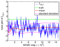
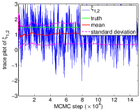
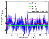
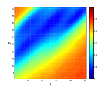
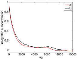
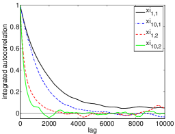
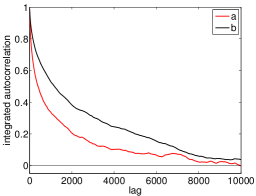
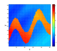
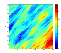
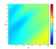
The true log-permeability $\log\kappa^{\dagger}$, shown in Figure 10 (top-left), is obtained from (26) with $\log\kappa_{1}^{\dagger}$ displayed in Figure 11 (top-left) $\log\kappa_{2}^{\dagger}$ shown in Figure 11 bottom-left and from $a^{\dagger}=0.11$ and $b^{\dagger}=0.86$. The functions $\log\kappa_{1}^{\dagger}$ and $\log\kappa_{2}^{\dagger}$ are draws from the Gaussian measures $N(m_{1},C_{1})$ and $N(m_{2},C_{2})$ that we use to define the prior (26). However, in order to avoid the inverse crime, these priors that we use to generate $\log\kappa_{1}^{\dagger}$ and $\log\kappa_{2}^{\dagger}$ (and so $u^{\dagger}$) are defined on a discretized domain (of $100\times 100$ grids) that is finer than the one used for the inversion. Synthetic data (data set 1) is generated by using the true permeability in the elliptic PDE and applying the measurement functional with 9 measurement locations as displayed in Figure 10 (bottom-left). Gaussian noise of standard deviation $\gamma=1.0\times 10^{-3}$ is added to the observations. For this case, we sample the posterior with the MCMC Algorithm 4.2 using the following splitting of the unknown $u=(a,b,\log\kappa_{1},\log\kappa_{2})$ for the outer Gibbs loop: (i) $\log\kappa_{1}$, (ii) $\log\kappa_{2}$ and (iii) $(a,b)$. Similar to the previous experiment, splitting the unknown yields the best performance in terms of decorrelation times. As before, 20 parallel chains were generated and the MPSRF was computed for assessing the convergence of the independent chains. Trace plots from one of these chains are presented in Figure 12. The samples from all chains were combined to produce the mean and variance of the unknown. The mean and variance of $\log\kappa_{1}$ and $\log\kappa_{2}$ are shown in Figure 11 (second column) and Figure 13, respectively (first column). The mean for the geometric parameters are $\hat{a}=0.198$ and $\hat{b}=0.639$. The corresponding variances are $\sigma_{a}=1.03\times 10^{-2}$ and $\sigma_{b}=9.5\times 10^{-3}$, respectively. The permeability (26) corresponding to the mean $\hat{u}$ is displayed in Figure 10 (top-middle).

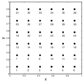
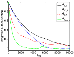
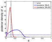
We repeat this experiment with a synthetic data (data set 2) that we now generate from a configuration of 36 measurement locations as specified in Figure 10 (bottom-right). Mean and variance of $\log\kappa_{1}$ and $\log\kappa_{2}$ are displayed in Figure 11 (third column) and Figure 13 (second column), respectively. The mean and variances for the geometric parameters are $\hat{a}=0.088$ and $\hat{b}=0.822$ and $\sigma_{a}=8\times 10^{-4}$ and $\sigma_{b}=7\times 10^{-4}$, respectively. The permeability (26) corresponding to the mean $\hat{u}$ is displayed in Figure 10 (top-right).

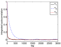
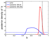
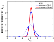
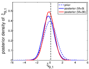
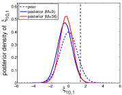
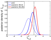
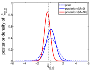
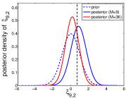
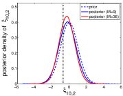
For both experiments, Figure 14 shows the autocorrelation of the geometric parameters as well as the KL-coefficients $\xi_{1,i}$ and $\xi_{10,i}$ from (28). In Figure 15 we present the posterior and the prior densities for geometric parameters and the aforementioned KL coefficients. From this figure we note that for some of the components of the unknown (e.g. $a$, $b$, $\xi_{1,2}$), the corresponding posterior density tends to be more peaked around the truth when more measurements are assimilated. Some less sensitive parameters seemed to be unaffected when more measurements are included. In particular, we see that the densities for the coefficients of smaller eigenvalues (e.g. $\xi_{9,2}$, $\xi_{10,2}$) for the permeability in $D_{2}$ is almost identical to the prior; indicating the uninformative effect of the data.

Figure 9: $\log\kappa$’s defined by (26) from samples of the prior (top row), posterior with fewer measurements (middle row) and posterior with more measurements (bottom-row)

Figure 10: Top, from left to right: truth, mean (fewer measurements), mean (more measurements) of $\log\kappa$. Bottom: measurement locations for data with less (left) and more (right) measurements.

Figure 11: Top: $\log\kappa_{1}$. Bottom: $\log\kappa_{2}$. From left to right: truth, mean (fewer measurements), mean (more measurements).

Figure 12: Trace plot from one MCMC chain (data 1). Top: geometric parameters. Bottom: Some KL modes of $\log\kappa_{1}$ and $\log\kappa_{2}$

Figure 13: Top to bottom: fewer measurements to more measurements. Left to right: variance of $\log\kappa_{1}$, Right: variance $\log\kappa_{2}$.

Figure 14: Autocorrelation from one MCMC chain. Top: data 1. Bottom: data 2. Left: geometric parameters. Right: Some KL model of $\log\kappa_{1}$ and $\log\kappa_{2}$

Figure 15: Prior and posterior densities of the unknown $u$

5.3 Channelized Permeability

In this experiment we consider channelized permeabilities of the form (26) where $D_{1}$ and $D_{2}$ are the domains corresponding to the interior and exterior of the channel, respectively. These domains are parametrized with five parameters as shown in Figure 2(b). Two fields for $\log\kappa_{i}$ are considered as in the previous experiments. The unknown parameter in this case is $u=(d_{1},\dots,d_{5},\log\kappa_{1},\log\kappa_{2})\in\mathbb{R}^{5}\times C({\overline{D}};\mathbb{R}^{2})$. We consider a prior distribution of the form

$$\mu_{0}(du)=\Pi_{i=1}^{5}\pi_{0}^{B_{i},g}(d_{i})\otimes N(m_{1},C_{1})N(m_{2},C_{2})$$ (29)

where the set $B_{i}$ in the definition of $\pi_{0}^{B_{i},g}(\cdot)$ (for each parameter) is a specified interval in $\mathbb{R}$, and $C_{1}$ and $C_{2}$ are covariance operators as in the previous experiment.

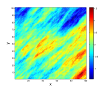
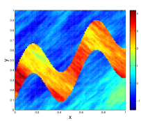
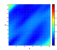
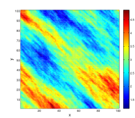
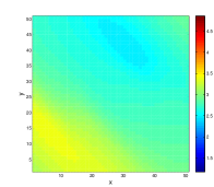
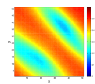
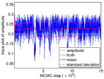
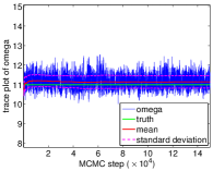
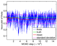
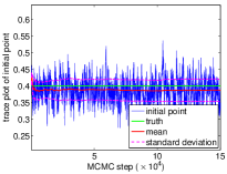
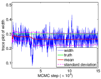
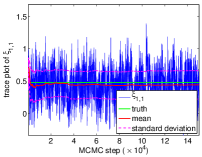
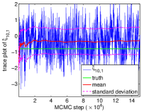
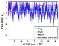
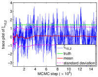
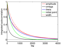
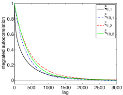
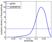
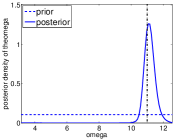
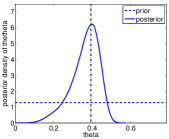
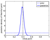
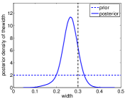
The true log-permeability $\log\kappa^{\dagger}$, shown in Figure 16 (left), is obtained from (26) with $\log\kappa_{1}^{\dagger}$ displayed in Figure 17 (top-left) $\log\kappa_{2}^{\dagger}$ shown in Figure 17 (bottom-left) and from the geometric parameters specified in Table 2. The true fields $\log\kappa_{i}^{\dagger}$ are generated as described in the preceding subsection. We consider the measurement configuration displayed in Figure 16 (right) and generate synthetic data as before. For the present example, the measurements are corrupted with noise with standard deviation of $\gamma=2.5\times 10^{-4}$. Algorithm 4.2 is applied to characterize the posterior distribution with 20 parallel chains that passed Gelman-Rubin MPSRF diagnostic [2]. For this experiment, we use an outer Gibbs loop in which we update each of the geometric parameters independently; then, both log-permeabilities field are updated simultaneously. Combined samples from all chains are used to compute the mean and variance of the unknown. Trace plots can be found in Figure 18. In Figure 19 we show log-permeabilities with parameter $u$ sampled from the prior (29) (top row) and the posterior (bottom row) respectively. In Figure 17 we show the posterior mean and variance for the fields $\log\kappa_{1}$ (second column) and $\log\kappa_{2}$ (third column), respectively. The mean and variance for the geometric parameters are reported in Table 2. The permeability (26) corresponding to the mean $\hat{u}$ is displayed in Figure 16 (middle). The autocorrelation of the geometric parameters and KL-coefficients $\xi_{1,i}$ and $\xi_{10,i}$ are shown in Figure 20. For these variables, in Figure 21 we display the posterior and the prior densities. Similar to our previous experiments, we observe that the log-permeability obtained with the mean parameters resembles the truth. However, the uncertainty in the problem is reflected in the variability in the possible inverse estimates of the log-permeability.

parameter	true value	mean	variance
(amplitude)	$0.2$	0.225	$1.3\times 10^{-3}$
(frecuency)	$11$	11.161	$1.12\times 10^{-1}$
(angle)	$0.39$	0.363	$5.3\times 10^{-3}$
(initial point)	$0.4$	0.388	$1.2\times 10^{-3}$
(width)	$0.3$	0.262	$1.6\times 10^{-3}$

Table 2: Data relevant to the experiment with the channelized permeability.

Figure 16: Left: true $\log\kappa$. Middle: mean $\log\kappa$. Right: Measurement configuration.

Figure 17: From left to right: truth, mean and variance of $\log\kappa_{1}$ (top) and $\log\kappa_{2}$ (bottom)

Figure 18: Trace plots from one MCMC chain.

Figure 19: $\log\kappa$’s defined by (26) (for the channelized geometry) from samples of the prior (top row) and the posterior(bottom-row)

Figure 20: Autocorrelation from one MCMC chain. Left: geometric parameters. Right: Some KL model of $\log\kappa_{1}$ and $\log\kappa_{2}$

Figure 21: Prior and posterior densities of the unknown $u$

6 Conclusion

The Bayesian framework provides a rigorous quantification of the uncertainty in the solution to the inverse problem of estimating rock properties given data from the subsurface flow. A key aspect of the proposed Bayesian approach is to incorporate prior knowledge that honors geometric features relevant to the characterization of complex geologic properties of the subsurface. Although other authors have considered geometrically defined priors, see for example [14, 34, 31, 4, 41], this is the first paper to give a rigorous function-space based Bayesian formulation for such problems [39]. Such formulations lead to the development of improved algorithms and allow for rigorous estimation of the various approximation errors that necessarily enter into the Bayesian approximation of inverse problems. In the present work we establish the existence and well-posedness of the Bayesian posterior that arises from determination of permeability within a Darcy flow model, define function-space MCMC methods, which therefore have convergence rates independent of the level of mesh-refinement used, and demonstrate the efficacy of these methods on a variety of test problems exhibiting faults, channels and spatial variability within different parts of the rock formations. Particular highlights of the work include: (i) the introduction of a novel Metropolis-within-Gibbs methodology which separates the effect of parameters describing the geometry from those describing spatial variability to accelerate convergence and does not require adjoint solves, only forward model runs; (ii) demonstration of choices of prior on the permeability values which lead to Hölder, but not Lipshitz, continuity of the posterior distribution with respect to perturbations in the data.

Our results indicate that the mean of the posterior often produce parameters whose permeabilities resemble the truth. However, substantial uncertainty in the inverse problem arises from the observational noise and the lack of observations. Increasing the accuracy in the data or increasing the measurement locations resulted in a significant decrease in the uncertainty in the inverse problem. In other words, we obtained posterior densities concentrated around the truth. In contrast to deterministic inverse problems where a variational optimization method is implemented to recover the truth, the proposed application of the Bayesian framework provides a derivative free method that produces a reasonable estimate of the truth alongside with an accurate estimate of its uncertainty. The present study indicates that the Bayesian framework herein, and resulting algorithmic approaches, have the potential to be applied to more complex flow models and geometries arising in subsurface applications where uncertainty quantification is required.

There are a number of natural directions in which this work might be extended. As mentioned earlier in the text, the study of model error is potentially quite fruitful: there is substantial gain in computational expediency stemming from imposing simple models of the geometry; determining how this is balanced by loss of accuracy when the actual data contains more subtle geometric effects, not captured our models, is of interest. It is also of interest to consider implementation of reversible jump type algorithms [18], in cases where the number of geometric parameters (e.g. the number of layers) is not known. And finally it will be of interest to construct rigorous Bayesian formulation of geometric inverse problems where the interfaces are functions, and require an infinite set of parameters to define them. We also highlight the fact that although we emphasize the importance of MCMC methods which are mesh-independent this does not mean that we have identified the definitive version of such methods; indeed it would be very interesting to combine our mesh-independent approach with other state-of-the art ideas in MCMC sampling such as adaptivity and delayed acceptance, which are used in the context of geophysical applications in [9], and Riemannian manifold methods [17], which also give rise to a natural adaptivity.

7 Appendix

Proof of Theorem 2.2.

Since $L$ comprises a finite number of linear functionals it suffices to prove continuity of the solution $p$ to (1) with respect to changes in the parameters $u$ which define $\kappa.$ Assuming $p$ (resp. $p^{\varepsilon}$) is the solution of (1) with $f\in V^{*}$ and diffusion coefficient $\kappa\in X$ (resp. $\kappa^{\varepsilon}\in X$) we first show that

$$\|p^{\varepsilon}-p\|_{V}\leq\frac{1}{\kappa^{\varepsilon}_{min}}\left(\int_{D}|\kappa^{\varepsilon}-\kappa|^{2}|\nabla p|^{2}dx\right)^{\frac{1}{2}}.$$ (30)

Define $e=p^{\varepsilon}-p$, $d=\kappa^{\varepsilon}-\kappa$. Then by (1) we have that $e\in H_{0}^{1}(D)$, $d\in L^{\infty}(D)$ satisfy

$$-\nabla\cdot(\kappa^{\varepsilon}\nabla e) =\nabla\cdot(d\nabla p),\quad x\in D$$

$$\phantom{-\nabla\cdot(\kappa^{\varepsilon}(x}e =0,\quad x\in\partial D.$$

Integration by parts gives

$$\int_{D}\kappa^{\varepsilon}\nabla e\cdot\nabla edx=-\int_{D}d\nabla p\cdot\nabla edx.$$

Hence,

$$\kappa^{\varepsilon}_{min}\|e\|^{2}_{V}\leq\int_{D}|d\nabla p\cdot\nabla e|dx\leq\int_{D}|d||\nabla p||\nabla e|dx\leq\left(\int_{D}d^{2}|\nabla p|^{2}dx\right)^{\frac{1}{2}}\|e\|_{V},$$

therefore (30) holds. Now, by (4) we have

$$\kappa^{\varepsilon}-\kappa=\sum_{i=1}^{n}\sum_{j=1}^{n}(\kappa_{j}^{\varepsilon}(x)-\kappa_{i}(x))\chi_{D_{j}^{\varepsilon}\cap D_{i}}(x).$$ (31)

Substituting (31) into (30), we obtain that

$$\|p^{\varepsilon}-p\|_{V} \leq\frac{1}{\kappa^{\varepsilon}_{min}}\left(\sum_{i=1}^{n}\sum_{j=1}^{n}\int_{D_{j}^{\varepsilon}\cap D_{i}}|\kappa_{j}^{\varepsilon}(x)-\kappa_{i}(x)|^{2}|\nabla p|^{2}dx\right)^{\frac{1}{2}}$$

$$\leq\frac{1}{\kappa^{\varepsilon}_{min}}\Big{(}\sum_{i=1}^{n}\|\kappa_{i}^{\varepsilon}-\kappa_{i}\|_{X}^{2}\int_{D_{i}^{\varepsilon}\cap D_{i}}|\nabla p|^{2}dx+\sum_{i\neq j}\|\kappa_{j}^{\varepsilon}-\kappa_{i}\|_{X}^{2}\int_{D_{j}^{\varepsilon}\cap D_{i}}|\nabla p|^{2}dx\Big{)}^{\frac{1}{2}}$$

$$\leq\frac{1}{\kappa^{\varepsilon}_{min}}\Big{(}\sum_{i=1}^{n}\|\kappa_{i}^{\varepsilon}-\kappa_{i}\|_{X}^{2}\int_{D_{i}^{\varepsilon}\cap D_{i}}|\nabla p|^{2}dx+\sum_{i\neq j}2\bigl{(}\|\kappa_{j}^{\varepsilon}\|_{X}^{2}+\|\kappa_{i}\|_{X}^{2}\bigr{)}\int_{D_{j}^{\varepsilon}\cap D_{i}}|\nabla p|^{2}dx\Big{)}^{\frac{1}{2}}.$$

The first term on the right hand side goes to zero as $\varepsilon\to 0$ because $p\in V$ and small changes in $u\in U\subset\mathcal{B}$, measured with respect to the norm $\|\cdot\|_{{\mathcal{B}}}$, lead to small changes in the $\kappa_{i}$ in $X$ for both the constant and continuous function models. Since Hypothesis 2.1 holds for all these geometric models of the domains $D_{i}$, and because $p\in V$, the dominated convergence theorem shows that

$$\int_{D_{j}^{\varepsilon}\cap D_{i}}|\nabla p|^{2}dx=\int_{D}\chi_{D_{j}^{\varepsilon}\cap D_{i}}|\nabla p|^{2}dx\to 0$$

as $\varepsilon\to 0$. Thus the second term goes to zero since $\kappa_{i}$ and $\kappa_{j}^{\varepsilon}$ are bounded on bounded subsets of $X$. ∎

Lemma 7.1.

Assume that $\kappa(x)$ is a piecewise constant function corresponding to parameter $u\in U\subset\mathcal{B}$. Let $\Phi(u;y)$ be the model-data misfit function in (10) and assume that $y,y^{\prime}\in Y$ with $\max\{|y|_{\Gamma},|y^{\prime}|_{\Gamma}\}<r$. If the prior $\mu_{0}$ on $u$ is constructed from the exponential distribution on the values of the $\kappa_{i}$, then for any $\iota\in(0,1)$, $\int_{U}M^{\iota}(r,u)d\mu_{0}<\infty,$ and

$$\int_{U}|\Phi(u;y)-\Phi(u,y^{\prime})|^{\iota}d\mu_{0}\leq C~{}|y-y^{\prime}|_{\Gamma}^{\iota},$$ (32)

where $C=\int_{U}M^{\iota}(r,u)d\mu_{0}$.

Proof.

By the Lax-Milgram Theorem, we have

$$|\mathcal{G}(u)|_{\Gamma} \leq\frac{C}{\min_{i}\{\kappa_{i}\}}=C\max_{i}\{\kappa_{i}^{-1}\},$$

which yields

$$\int_{U}M^{\iota}(r,u)d\mu_{0}\leq\int_{U}\left(r+C\max_{i}\{\kappa_{i}^{-1}\}\right)^{\iota}d\mu_{0}$$

$$=\int_{\{r>C\max_{i}\{\kappa_{i}^{-1}\}\}}\left(r+C\max_{i}\{\kappa_{i}^{-1}\}\right)^{\iota}d\mu_{0}+\int_{\{r\leq C\max_{i}\{\kappa_{i}^{-1}\}\}}\left(r+C\max_{i}\{\kappa_{i}^{-1}\}\right)^{\iota}d\mu_{0}$$

$$\leq(2r)^{\iota}\mu_{0}\left({\{r>C\max_{i}\{\kappa_{i}^{-1}\}\}}\right)+(2C)^{\iota}\int_{U}\max_{i}\{\kappa_{i}^{-\iota}\}d\mu_{0}<\infty.$$

The second term of the right hand side is finite, since when $\iota\in(0,1)$,

$$\int_{U}\max_{i}\{\kappa_{i}^{-\iota}\}d\mu_{0}\leq\int_{U}\sum_{i=1}^{n}\frac{1}{\kappa_{i}^{\iota}}d\mu_{0}=\sum_{i=1}^{n}\int_{0}^{+\infty}\lambda_{i}\frac{1}{\kappa_{i}^{\iota}}\exp(-\lambda_{i}\kappa_{i})d\kappa_{i}$$

$$\leq\sum_{i=1}^{n}\lambda_{i}\left(\int_{0}^{1}\frac{1}{\kappa_{i}^{\iota}}d\kappa_{i}+\int_{1}^{+\infty}\exp(-\lambda_{i}\kappa_{i})d\kappa_{i}\right)<\infty.$$

Therefore, by (18) we obtain

$$\int_{U}|\Phi(u;y)-\Phi(u,y^{\prime})|^{\iota}d\mu_{0}\leq\int_{U}M^{\iota}(r,u)d\mu_{0}~{}|y-y^{\prime}|_{\Gamma}^{\iota}.$$

∎

Lemma 7.2.

Assume that $\kappa(x)$ is a piecewise constant function corresponding to parameter $u\in U\subset\mathcal{B}$. Let $\mu_{0}$ be the prior distribution on $U$ and such that the values of permeability $\kappa_{i}$ are drawn from the exponential distribution. Then for any $\iota\in(0,1)$,

$$\mu_{0}\left(|\Phi(u;y)-\Phi(u,y^{\prime})|>1\right)\leq\int_{U}M^{\iota}(r,u)d\mu_{0}~{}|y-y^{\prime}|_{\Gamma}^{\iota}.$$

Proof.

By the Markov inequality we have

$$\mu_{0}\left(|\Phi(u,y)-\Phi(u,y^{\prime})|>1\right)=\mu_{0}\left(\frac{1}{2}\left|\langle y-y^{\prime},y+y^{\prime}-2\mathcal{G}(u)\rangle_{\Gamma}\right|>1\right)$$

$$\leq\mu_{0}\left(\left|y-y^{\prime}\right|_{\Gamma}\left|y+y^{\prime}-2\mathcal{G}(u)\right|_{\Gamma}>2\right)=\mu_{0}\left(\left|y+y^{\prime}-2\mathcal{G}(u)\right|_{\Gamma}>\frac{2}{\left|y-y^{\prime}\right|_{\Gamma}}\right)$$

$$\leq\frac{\left|y-y^{\prime}\right|_{\Gamma}^{\iota}}{2^{\iota}}\int_{U}\left|y+y^{\prime}-2\mathcal{G}(u)\right|_{\Gamma}^{\iota}~{}\mathrm{d}\mu_{0}\leq\frac{\left|y-y^{\prime}\right|_{\Gamma}^{\iota}}{2^{\iota}}\int_{U}2^{\iota}\left(r+|\mathcal{G}(u)|_{\Gamma}\right)^{\iota}~{}\mathrm{d}\mu_{0}$$

$$\leq\left|y-y^{\prime}\right|_{\Gamma}^{\iota}\int_{U}M^{\iota}(r,u)~{}\mathrm{d}\mu_{0}$$

∎

Proof of Proposition 4.1.

In order to construct a prior-reversible proposal for density $\pi_{0}(u)$ on $U$ we first extend this density to a target on the whole of $\mathbb{R}^{d}$ by setting the density to zero outside $U$. We then draw $w$ from $p(u,w)$ and define $v$ according to

$$v=\left\{\begin{array}[]{cc}w&\mathrm{with~{}probability}~{}a(u,w)\\ u&\mathrm{otherwise}\end{array}\right.,$$ (33)

where

$$a(u,w)=\frac{\pi_{0}(w)p(w,u)}{\pi_{0}(u)p(u,w)}\wedge 1.$$

Together these steps define a Markov kernel $q(u,v)$ on $U\times U$ which is $\pi_{0}$ reversible. Furthermore, as we now show, the method reduces to that given in Proposition 4.1. Because of the property (23) of $p$ we have that, if $u\in U$, $w\in U$ then

$$a(u,w)=\frac{\pi_{0}(w)p(w,u)}{\pi_{0}(u)p(u,w)}\wedge 1=1.$$

If $u\in U$, $w\notin U$ then

$$a(u,w)=\frac{\pi_{0}(w)p(w,u)}{\pi_{0}(u)p(u,w)}\wedge 1=0\wedge 1=0.$$

Therefore, if $u\in U$, then

$$a(u,w)=\left\{\begin{array}[]{ll}1&w\in U\\ 0&w\notin U\end{array}\right.,$$

and the Metropolis-Hastings algorithm (33) simplifies to give the process where $w$ is drawn from $p(u,w)$ and we set

$$v=\left\{\begin{array}[]{ll}w&w\in U\\ u&w\notin U\end{array}\right..$$

This coincides with what we construct for $q(u,v)$ in (22). Hence, the process in (22) is actually generated by a Metropolis-Hastings algorithm for target distribution $\pi_{0}(u)$. By the theory of Metropolis-Hastings algorithms, we know that $q(u,v)$ will be reversible with respect to the equilibrium distribution $\pi_{0}$. ∎

References

- [1] A. Beskos, G. Roberts, A. M. Stuart, and J. Voss. MCMC methods for diffusion bridges. Stochastics and Dynamics, 8(03):319–350, 2008.
- [2] S. P. Brooks and A. Gelman. General methods for monitoring convergence of iterative simulations. Journal of Computational and Graphical Statistics, 7:434–455, December 1998.
- [3] J. N. Carter and D. A. White. History matching on the Imperial College fault model using parallel tempering. Computational Geosciences, 17:43–65, 2013.
- [4] H. Chang, D. Zhang, and Z. Lu. History matching of facies distribution with the enkf and level set parameterization. J. Comput. Phys., 229(20):8011–8030, October 2010.
- [5] S. L. Cotter, M. Dashti, J. C. Robinson, and A. M. Stuart. Bayesian inverse problems for functions and applications to fluid mechanics. Inverse Problems, 25:doi:10.1088/0266–5611/25/11/115008, 2009.
- [6] S. L. Cotter, M. Dashti, and A. M. Stuart. Approximation of Bayesian inverse problems for PDEs. SIAM Journal on Numerical Analysis, 48(1):322–345, 2010.
- [7] S. L. Cotter, M. Dashti, and A. M. Stuart. Variational data assimilation using targetted random walks. Int. J. Num. Meth. Fluids, 68(4):403–421, 2012.
- [8] S. L. Cotter, G. O. Roberts, A. M. Stuart, and D. White. MCMC methods for functions: Modifying old algorithms to make them faster. Statistical Science, 28(3):424–446, 08 2013.
- [9] T Cui, C Fox, and MJ O’Sullivan. Bayesian calibration of a large-scale geothermal reservoir model by a new adaptive delayed acceptance metropolis hastings algorithm. Water Resources Research, 47(10), 2011.
- [10] M. Dashti, S. Harris, and A. M. Stuart. Besov priors for Bayesian inverse problems. Inverse Problems and Imaging, 6:183–200, 2012.
- [11] M. Dashti and A. M. Stuart. Uncertainty quantification and weak approximation of an elliptic inverse problem. SIAM J. Num. Anal., 49:2524–2542, 2011.
- [12] O. Dorn and D. Lesselier. Level set methods for inverse scattering-some recent developments. Inverse Problems, 25(12):125001, 2009.
- [13] O. Dorn and R. Villegas. History matching of petroleum reservoirs using a level set technique. Inverse Problems, 24(3):035015, 2008.
- [14] Y. Efendiev, A. Datta-Gupta, X. Ma, and B. Mallick. Efficient sampling techniques for uncertainty quantification in history matching using nonlinear error models and ensemble level upscaling techniques. Water Resources Research, 45(W11414):11pp, 2009.
- [15] A. A. Emerick and A. C. Reynolds. Investigation of the sampling performance of ensemble-based methods with a simple reservoir model. Computational Geosciences, 17(2):325–350, 2013.
- [16] J. N. Franklin. Well-posed stochastic extensions of ill-posed linear problems. Journal of Mathematical Analysis and Applications, 31(3):682–716, 1970.
- [17] M. Girolami and B. Calderhead. Riemann manifold langevin and hamiltonian monte carlo methods. Journal of the Royal Statistical Society: Series B (Statistical Methodology), 73(2):123–214, 2011.
- [18] P. J. Green. Reversible jump markov chain monte carlo computation and bayesian model determination. Biometrika, 82(4):711–732, 1995.
- [19] M. Hairer, A. M. Stuart, and S. J. Vollmer. Spectral gaps for Metropolis-Hastings algorithms in infinite dimensions. Ann. Appl. Prob. To Appear.
- [20] M. A. Iglesias, K. J. H. Law, and A. M. Stuart. Evaluation of Gaussian approximations for data assimilation in reservoir models. Computational Geosciences, pages 1–35, 2013.
- [21] M. A. Iglesias and D. McLaughlin. Level-set techniques for facies identification in reservoir modeling. Inverse Problems, 27:035008, 2011.
- [22] J. P. Kaipio, V. Kolehmainen, M. Vauhkonen, and E. Somersalo. Inverse problems with structural prior information. Inverse problems, 15(3):713, 1999.
- [23] J. P. Kaipio and E. Somersalo. Statistical inverse problems: discretization, model reduction and inverse crimes. J. Comp. Appl. Math., 198:493–504, 2007.
- [24] J. Landa and R. Horne. A procedure to integrate well test data, reservoir performance history and 4-d seismic information into a reservoir description. in Proccedings of the SPE Annual Technical Conference and Exhibition, 5-8 October 1997, San Antonio, Texas, U.S.A., SPE 38653, 1997.
- [25] S. Lasanen. Discretizations of generalized random variables with applications to inverse problems. Ann. Acad. Sci. Fenn. Math. Diss., University of Oulu, 130, 2002.
- [26] S. Lasanen. Non-Gaussian statistical inverse problems. Part I: Posterior distributions. Inverse Problems and Imaging, 6(2):215–266, 2012.
- [27] S. Lasanen. Non-Gaussian statistical inverse problems. Part II: Posterior convergence for approximated unknowns. Inverse Problems and Imaging, 6(2):267–287, 2012.
- [28] M. Lassas, E. Saksman, and S. Siltanen. Discretization-invariant Bayesian inversion and Besov space priors. Inverse Problems and Imaging, 3:87–122, 2009.
- [29] M. S. Lehtinen, L. Päivärinta, and E. Somersalo. Linear inverse problems for generalised random variables. Inverse Problems, 5(4):599–612, 1989.
- [30] N. Liu and D. S. Oliver. Evaluation of Monte Carlo methods for assessing uncertainty. SPE J., 8:188–195, 2003.
- [31] N. Liu and D. S. Oliver. Ensemble Kalman filter for automatic history matching of geologic facies. Journal of Petroleum Science and Engineering, 47(3–4):147 Р161, 2005.
- [32] A. Mandelbaum. Linear estimators and measurable linear transformations on a Hilbert space. Z. Wahrsch. Verw. Gebiete, 65(3):385–397, 1984.
- [33] Y. Marzouk and D. Xiu. A stochastic collocation approach to Bayesian inference in inverse problems. Communications in Computational Physics, 6:826–847, 2009.
- [34] A. Mondal, Y. Efendiev, B. Mallick, and A. Datta-Gupta. Bayesian uncertainty quantification for flows in heterogeneous porous media using reversible jump Markov chain Monte Carlo methods. Advances in Water Resources, 33(3):241 – 256, 2010.
- [35] R. Neal. Regression and classification using Gaussian process priors. In Bayesian Statistics, pages 475–501, 2010.
- [36] D. Oliver and Y. Chen. Recent progress on reservoir history matching: a review. Computational Geosciences, 15:185–221, 2011. 10.1007/s10596-010-9194-2.
- [37] D. S. Oliver, A. C. Reynolds, and N. Liu. Inverse Theory for Petroleum Reservoir Characterization and History Matching. Cambridge University Press, ISBN: 9780521881517, 1st edition, 2008.
- [38] A. M. Stuart. The Bayesian Approach to Inverse Problems. Lecture Notes, arXiv:1302.6989.
- [39] A. M. Stuart. Inverse problems: a Bayesian perspective. Acta Numerica, 19(1):451–559, 2010.
- [40] S. Vollmer. Dimension-independent MCMC sampling for elliptic inverse problems with non-Gaussian priors. 2013. arXiv preprint, arXiv:1302.2213.
- [41] J. Xie, Y. Efendiev, and A. Datta-Gupta. Uncertainty quantification in history matching of channelized reservoirs using Markov chain level set approaches. in Proccedings of the SPE Reservoir Simulation Symposium, 21-23 February 2011, The Woodlands, Texas, USA, SPE 141811, 2011.
- [42] B. Zhuoxin, D. S. Oliver, and A. C. Reynolds. Conditioning 3d stochastic channels to pressure data. SPE Journal, 5(4):474–484, 2000.