1 Introduction
Determinantal point processes ( [ 22 ] ) have played a central role in recent developments of many random models such as random matrix theory, random growth and tiling problems (see for example [ 3 ] , [ 17 ] , [ 19 ] ).
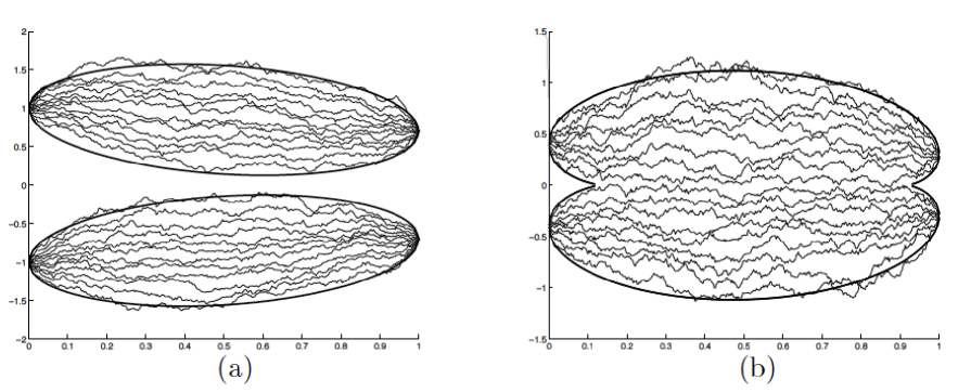
One of the most well-known model for determinantal point process is the case of n 𝑛 n Brownian particles moving on the real line, conditioned never to intersect, with given starting and ending configuration. Let’s assume that all the particles start at two given fixed points and end at two other points (which may coincide with the starting points). As time runs in an interval t ∈ [ 0 , 1 ] 𝑡 0 1 t\in[0,1] ( 1 1 1 being the end time where the particles collapse in the two final points), the particles remain confined in a specific region and for every time t ∈ [ 0 , 1 ] 𝑡 0 1 t\in[0,1] the positions of the Brownian paths form a determinantal process.
Moreover, as the number of particles tends to infinity, such region takes on an explicit shape which depends on the relative position of the starting and ending points and on a parameter σ 𝜎 \sigma which controls the strength of interaction between the left-most particles and the right-most ones ( σ 𝜎 \sigma can be thought as a pressure or temperature parameter).
There are two possible scenarios: two independent connected components similar to ellipses, one connected component similar to two “merged” ellipses (see Figure 1 , case ( a ) 𝑎 (a) and ( b ) 𝑏 (b) ).
It is well-known that the microscopic behaviour of such infinite particle system is regulated by the Sine process in the bulk of the particle bundles ( [ 21 ] ), by the Airy process along the soft edges ( [ 19 ] , [ 18 ] , [ 23 ] ) and by the Pearcey process in the cusp singularity ( [ 24 ] ), when it occurs.
Figure 1: Non-intersecting Brownian motions with two starting points ± α plus-or-minus 𝛼 \pm\alpha ± β plus-or-minus 𝛽 \pm\beta ( a ) 𝑎 (a) ( b ) 𝑏 (b) ( c ) 𝑐 (c) n → ∞ → 𝑛 n\rightarrow\infty t ∈ [ 0 , 1 ] 𝑡 0 1 t\in[0,1] n = 20 𝑛 20 n=20 ( a ) 𝑎 (a) α = 1 , β = 0.7 formulae-sequence 𝛼 1 𝛽 0.7 \alpha=1,\beta=0.7 ( b ) 𝑏 (b) α = 0.4 , β = 0.3 formulae-sequence 𝛼 0.4 𝛽 0.3 \alpha=0.4,\beta=0.3 ( c ) 𝑐 (c) α = 1 , β = 0.5 formulae-sequence 𝛼 1 𝛽 0.5 \alpha=1,\beta=0.5 [13 ] .
There exist a third critical configuration, which can be seen as a limit of the large separation case when the two bundles are tangential to each other in one point, called tacnode point (see Figure 1 , case ( c ) 𝑐 (c) ). In a microscopic neighbourhood of this point the fluctuations of the particles are described by a new critical process called Tacnode process.
The kernel of such process in the single-time case has been first introduced by Kuijlaars et al. in [ 10 ] , where the kernel was expressed in terms of a 4 × 4 4 4 4\times 4 matrix valued Riemann-Hilbert problem. Shortly after Kuijlaars’s paper, Johansson formulated the multi-time (or extended) version of the process ( [ 20 ] ), remarking nevertheless the fact that this extended version does not automatically reduce to the single-time version given in [ 10 ] . The kernel was expressed in terms of resolvents and Fredholm determinants of the Airy operator acting on a semi-infinite interval [ σ , ∞ ) 𝜎 [\sigma,\infty) . Another version of the multi-time Tacnode process was given in [ 1 ] .
In [ 2 ] the authors analyzed the same process as arising from random tilings instead of self-avoiding Brownian paths and they proved the equivalency of all the above formulations.
A similar result has been obtained by Delvaux in [ 9 ] , where a Riemann-Hilbert expression for the multi-time tacnode kernel is given. A more general formulation of this process has been studied in [ 11 ] , where the limit shapes of the two groups of particles are allowed to be non-symmetric.
Physically, if we start from the tacnode configuration and we push together the two ellipses, they will merge giving rise to the single connected component in Figure 1 ( b ) 𝑏 (b) , while if we pull the ellipses apart, we simply end up with two disjoint ellipses as in Figure 1 ( c ) 𝑐 (c) . It is thus natural to expect that the local dynamic around the tacnode point will in either cases degenerates into a Pearcey process or an Airy process, respectively.
The degeneration Tacnode-Pearcey has been proven in [ 13 ] where the authors showed a uniform convergence of the Tacnode kernel to the Pearcey kernel over compact sets in the limit as the pressure parameter diverges to − ∞ -\infty . On the other hand, the method used in [ 13 ] cannot be extensively applied to the Tacnode-Airy degeneration, since the Airy process can be defined also on non-compact sets.
The purpose of the present paper is to study the asymptotic behaviour of the gap probability of the (single-time) Tacnode process and its degeneration into the gap probability of the Airy process.
There are two types of regimes in which this degeneration occurs:
the limit as σ → + ∞ → 𝜎 \sigma\rightarrow+\infty (large separation), which physically corresponds to pulling apart the two sets of Brownian particles touching on the tacnode point, and the limit as τ → ± ∞ → 𝜏 plus-or-minus \tau\rightarrow\pm\infty (large time), which corresponds to moving away from the singular point along the boundary of the space-time region swept out by the non-intersecting paths.
An expression for the single-time tacnode kernel is the following (see [ 2 , formula (19)] )
𝕂 tac ( τ ; x , y ) = superscript 𝕂 tac 𝜏 𝑥 𝑦
absent \displaystyle\mathbb{K}^{\rm tac}(\tau;x,y)=
K Ai ( τ , − τ ) ( σ − x , σ − y ) + 2 3 ∫ σ ~ ∞ d z ∫ σ ~ ∞ d w 𝒜 x − σ τ ( w ) ( Id − K Ai | [ σ ~ , + ∞ ) ) − 1 ( z , w ) 𝒜 y − σ − τ ( z ) subscript superscript 𝐾 𝜏 𝜏 Ai 𝜎 𝑥 𝜎 𝑦 3 2 superscript subscript ~ 𝜎 differential-d 𝑧 superscript subscript ~ 𝜎 differential-d 𝑤 subscript superscript 𝒜 𝜏 𝑥 𝜎 𝑤 superscript Id evaluated-at subscript 𝐾 Ai ~ 𝜎 1 𝑧 𝑤 subscript superscript 𝒜 𝜏 𝑦 𝜎 𝑧 \displaystyle K^{(\tau,-\tau)}_{\mathrm{Ai}}(\sigma-x,\sigma-y)+\sqrt[3]{2}\int_{\widetilde{\sigma}}^{\infty}{\rm d}z\int_{\widetilde{\sigma}}^{\infty}{\rm d}w\mathcal{A}^{\tau}_{x-\sigma}(w)\left(\operatorname{Id}-K_{\mathrm{Ai}}\bigg{|}_{[\widetilde{\sigma},+\infty)}\right)^{-1}(z,w){\mathcal{A}}^{-\tau}_{y-\sigma}(z) (1.1)
with σ ~ := 2 2 3 σ assign ~ 𝜎 superscript 2 2 3 𝜎 \widetilde{\sigma}:=2^{\frac{2}{3}}\sigma and
Ai ( τ ) ( x ) superscript Ai 𝜏 𝑥 \displaystyle\mathrm{Ai}^{(\tau)}(x) := e τ x + 2 3 τ 3 Ai ( x ) = ∫ γ R d λ 2 i π e λ 3 3 + λ 2 τ − x λ assign absent superscript e 𝜏 𝑥 2 3 superscript 𝜏 3 Ai 𝑥 subscript subscript 𝛾 𝑅 d 𝜆 2 𝑖 𝜋 superscript e superscript 𝜆 3 3 superscript 𝜆 2 𝜏 𝑥 𝜆 \displaystyle:={\rm e}^{\tau x+\frac{2}{3}\tau^{3}}\mathrm{Ai}(x)=\int_{\gamma_{R}}\frac{{\rm d}\lambda}{2i\pi}{\rm e}^{\frac{\lambda^{3}}{3}+\lambda^{2}\tau-x\lambda} (1.2)
Ai ( x ) Ai 𝑥 \displaystyle\mathrm{Ai}(x) := ∫ γ R d λ 2 i π e λ 3 3 − x λ = − ∫ γ L d λ 2 i π e − λ 3 3 + x λ assign absent subscript subscript 𝛾 𝑅 d 𝜆 2 𝑖 𝜋 superscript e superscript 𝜆 3 3 𝑥 𝜆 subscript subscript 𝛾 𝐿 d 𝜆 2 𝑖 𝜋 superscript e superscript 𝜆 3 3 𝑥 𝜆 \displaystyle:=\int_{\gamma_{R}}\frac{{\rm d}\lambda}{2i\pi}{\rm e}^{\frac{\lambda^{3}}{3}-x\lambda}=-\int_{\gamma_{L}}\frac{{\rm d}\lambda}{2i\pi}{\rm e}^{-\frac{\lambda^{3}}{3}+x\lambda} (1.3)
𝒜 x τ ( z ) subscript superscript 𝒜 𝜏 𝑥 𝑧 \displaystyle\mathcal{A}^{\tau}_{x}(z) := Ai ( τ ) ( x + 2 3 z ) − ∫ 0 ∞ d w Ai ( τ ) ( − x + 2 3 w ) Ai ( w + z ) assign absent superscript Ai 𝜏 𝑥 3 2 𝑧 superscript subscript 0 differential-d 𝑤 superscript Ai 𝜏 𝑥 3 2 𝑤 Ai 𝑤 𝑧 \displaystyle:=\mathrm{Ai}^{(\tau)}(x+\sqrt[3]{2}z)-\int_{0}^{\infty}{\rm d}w\,\mathrm{Ai}^{(\tau)}(-x+\sqrt[3]{2}w)\mathrm{Ai}(w+z) (1.4)
K Ai ( τ , − τ ) ( − x , − y ) superscript subscript 𝐾 Ai 𝜏 𝜏 𝑥 𝑦 \displaystyle K_{\mathrm{Ai}}^{(\tau,-\tau)}(-x,-y) : = ∫ 0 ∞ d u Ai ( τ ) ( − x + u ) Ai ( − τ ) ( − y + u ) \displaystyle:=\int_{0}^{\infty}{\rm d}u\mathrm{Ai}^{(\tau)}(-x+u)\mathrm{Ai}^{(-\tau)}(-y+u) (1.5)
K Ai ( z , w ) subscript 𝐾 Ai 𝑧 𝑤 \displaystyle K_{\mathrm{Ai}}(z,w) := ∫ 0 ∞ d u Ai ( z + u ) Ai ( w + u ) assign absent superscript subscript 0 differential-d 𝑢 Ai 𝑧 𝑢 Ai 𝑤 𝑢 \displaystyle:=\int_{0}^{\infty}\!\!\!\!{\rm d}u\,\mathrm{Ai}(z+u)\mathrm{Ai}(w+u) (1.6)
where the contour γ R subscript 𝛾 𝑅 \gamma_{R} is the contour extending to infinity in the λ 𝜆 \lambda -plane along the rays e ± i π 3 superscript 𝑒 plus-or-minus 𝑖 𝜋 3 {e}^{\pm i\frac{\pi}{3}} , oriented upwards and entirely contained in the right half plane ( ℜ ( λ ) > 0 𝜆 0 \Re(\lambda)>0 ), and γ L := − γ R assign subscript 𝛾 𝐿 subscript 𝛾 𝑅 \gamma_{L}:=-\gamma_{R} .
The quantity of interest, i.e. the gap probability of the process, is expressed in terms of the Fredhom determinant of an integral operator with kernel ( 1.1 ). Given a Borel set ℐ ℐ \mathcal{I} , then
P ( no particles in ℐ ) = det ( Id − 𝕂 tac | ℐ ) 𝑃 no particles in ℐ Id evaluated-at superscript 𝕂 tac ℐ P\left(\text{no particles in }\mathcal{I}\right)=\det\left(\operatorname{Id}-\mathbb{K}^{\rm tac}\bigg{|}_{\mathcal{I}}\right) (1.7)
The first difficulty in studying the Tacnode process is the expression of its kernel, since it is highly transcendental and it involves the resolvent of the Airy operator. It it thus necessary to reduce it to a more approachable form.
The first important step was [ 7 , Theorem 3.1] where it was proved that gap probabilities of the Tacnode process can be defined as ratio of two Fredholm determinants of explicit integral operators with kernels that only involves contour integrals, exponentials and Airy functions.
This result, which will be recalled in Section 3 , will be our starting point in the investigation of the gap probabilities and their asymptotics.
The second step will be to find an appropriate integral operator in the sense of Its-Izergin-Korepin-Slavnov ( [ 16 ] ) whose Fredholm determinant coincides with the quantity ( 1.7 ). In this way, it will be possible to give a formulation of the gap probabilities of the Tacnode in terms of a Riemann-Hilbert (RH) problem, naturally associated to an IIKS integral operator (see [ 15 ] ). Finally, applying well-known steepest descent methods to the above RH problem, we will be able to prove the conjectured degeneration into Airy processes.
The RH approach for studying gap probabilities has been extensively used in the past years. To cite a few, we recall the study of gap probabilities for the Airy and Pearcey kernels in [ 5 ] and [ 6 ] and for the Bessel kernel in [ 14 ] .
The outline of the paper is the following: in Section 2 we state the main results of the paper, which will be proved in Sections 3 , 4 and 5 . In particular, Section 3 deals with some preliminary calculations which are necessary to set a Riemann-Hilbert problem on which we shall later perform some steepest descent analysis in the limit as σ → ∞ → 𝜎 \sigma\rightarrow\infty (Section 4 ) or τ → ∞ → 𝜏 \tau\rightarrow\infty (Section 5 ).
2 Results
The first results on asymptotic regime of the tacnode process were stated in [ 7 ] . We are recalling them here for the sake of completeness.
Theorem 2.1 .
Let ℐ := ⋃ j = 1 K [ a 2 j − 1 , a 2 j ] assign ℐ superscript subscript 𝑗 1 𝐾 subscript 𝑎 2 𝑗 1 subscript 𝑎 2 𝑗 \mathcal{I}:=\bigcup_{j=1}^{K}[a_{2j-1},a_{2j}] a j = a ( s j ) = − σ − τ 2 + s j subscript 𝑎 𝑗 𝑎 subscript 𝑠 𝑗 𝜎 superscript 𝜏 2 subscript 𝑠 𝑗 a_{j}=a(s_{j})=-\sigma-\tau^{2}+s_{j} σ 𝜎 \sigma
lim τ → ± ∞ det ( Id − 𝕂 tac | ℐ ) = det ( Id − K Ai | J ) subscript → 𝜏 plus-or-minus Id evaluated-at superscript 𝕂 tac ℐ Id evaluated-at subscript 𝐾 Ai 𝐽 \lim_{\tau\rightarrow\pm\infty}\det\left(\operatorname{Id}-\mathbb{K}^{\rm tac}\bigg{|}_{\mathcal{I}}\right)=\det\left(\operatorname{Id}-K_{\mathrm{Ai}}\bigg{|}_{J}\right) (2.1)
with J = ⋃ ℓ = 1 K [ s 2 ℓ − 1 , s 2 ℓ ] 𝐽 superscript subscript ℓ 1 𝐾 subscript 𝑠 2 ℓ 1 subscript 𝑠 2 ℓ J=\bigcup_{\ell=1}^{K}[s_{2\ell-1},s_{2\ell}] τ 𝜏 \tau
lim σ → + ∞ det ( Id − 𝕂 tac | ℐ ) = det ( Id − K Ai | J ) subscript → 𝜎 Id evaluated-at superscript 𝕂 tac ℐ Id evaluated-at subscript 𝐾 Ai 𝐽 \lim_{\sigma\rightarrow+\infty}\det\left(\operatorname{Id}-\mathbb{K}^{\rm tac}\bigg{|}_{\mathcal{I}}\right)=\det\left(\operatorname{Id}-K_{\mathrm{Ai}}\bigg{|}_{J}\right) (2.2)
Proof.
The convergence follows easily by directly studying the kernel of the extended tacnode process (see [ 2 , formula (19)] ), since the term involving the resolvent of the Airy kernel tends to zero, uniformly over
compact sets of the spatial variables x − σ − τ 2 𝑥 𝜎 superscript 𝜏 2 x-\sigma-\tau^{2} .
∎
A more interesting situation is the one in which the tacnode process degenerates into a couple of Tracy-Widom distributions, in analogy with the Pearcey-to-Airy transition (see [ 6 ] ). In this case, half of the space variables (endpoints of the gaps) moves far away from the tacnode following the left branch of the boundary of the space-time region swept by the particles, and the other half goes in the opposite direction. Therefore, it is expected that the gap probability of the tacnode process for a “large gap” factorize into two Fredholm determinants for semi-infinite gaps of the Airy process.
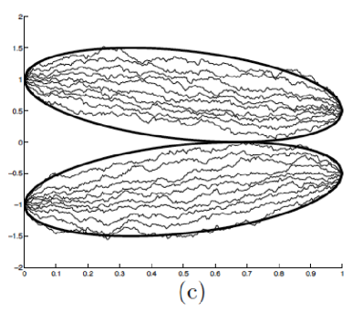
Numerically, these regimes are illustrated in Figure 2 . The results were already conjectured in [ 7 ] and they are here rigorously proved.
Figure 2: The relative values 1 − det ( Id − Π 𝕂 tac Π ) F 2 ( a ) F 2 ( b ) 1 Id Π superscript 𝕂 tac Π subscript 𝐹 2 𝑎 subscript 𝐹 2 𝑏 1-\frac{\det(\operatorname{Id}-\Pi\mathbb{K}^{\rm tac}\Pi)}{F_{2}(a)F_{2}(b)} Π Π \Pi [ a tac , b tac ] subscript 𝑎 tac subscript 𝑏 tac [a_{\rm tac},b_{\rm tac}] a tac = a − σ − τ t a c 2 subscript 𝑎 tac 𝑎 𝜎 subscript superscript 𝜏 2 𝑡 𝑎 𝑐 a_{\rm tac}=a-\sigma-\tau^{2}_{tac} b tac = − b + σ + τ t a c 2 subscript 𝑏 tac 𝑏 𝜎 superscript subscript 𝜏 𝑡 𝑎 𝑐 2 b_{\rm tac}=-b+\sigma+\tau_{tac}^{2} τ tac subscript 𝜏 tac \tau_{\rm tac} σ 𝜎 \sigma a = − 0.3 𝑎 0.3 a=-0.3 b = 0.5 𝑏 0.5 b=0.5 [7 ] .
In the simple case with only one interval, we have the following theorems.
Theorem 2.2 (Asymptotics as σ → + ∞ → 𝜎 \sigma\rightarrow+\infty ).
Let 𝕂 tac superscript 𝕂 tac \mathbb{K}^{\rm tac} K Ai subscript 𝐾 Ai K_{\mathrm{Ai}}
a = a ( t ) = − σ − τ 2 + t b = b ( s ) = σ + τ 2 − s formulae-sequence 𝑎 𝑎 𝑡 𝜎 superscript 𝜏 2 𝑡 𝑏 𝑏 𝑠 𝜎 superscript 𝜏 2 𝑠 a=a(t)=-\sigma-\tau^{2}+t\ \ \ b=b(s)=\sigma+\tau^{2}-s (2.3)
then as σ → + ∞ → 𝜎 \sigma\rightarrow+\infty
det ( Id − 𝕂 tac | [ − σ − τ 2 + t , σ + τ 2 − s ] ) = Id evaluated-at superscript 𝕂 tac 𝜎 superscript 𝜏 2 𝑡 𝜎 superscript 𝜏 2 𝑠 absent \displaystyle\det\left(\operatorname{Id}-\mathbb{K}^{\rm tac}\bigg{|}_{[-\sigma-\tau^{2}+t,\sigma+\tau^{2}-s]}\right)=
det ( Id − K Ai | [ s , + ∞ ) ) det ( Id − K Ai | [ t , + ∞ ) ) ( 1 + 𝒪 ( σ − 1 ) ) Id evaluated-at subscript 𝐾 Ai 𝑠 Id evaluated-at subscript 𝐾 Ai 𝑡 1 𝒪 superscript 𝜎 1 \displaystyle\det\left(\operatorname{Id}-K_{\mathrm{Ai}}\bigg{|}_{[s,+\infty)}\right)\det\left(\operatorname{Id}-K_{\mathrm{Ai}}\bigg{|}_{[t,+\infty)}\right)\left(1+\mathcal{O}(\sigma^{-1})\right) (2.4)
and the convergence is uniform over compact sets of the variables s , t 𝑠 𝑡
s,t
− ∞ < s , t < K 1 ( σ + τ 2 ) , 0 < K 1 < 1 . formulae-sequence 𝑠 formulae-sequence 𝑡 subscript 𝐾 1 𝜎 superscript 𝜏 2 0 subscript 𝐾 1 1 -\infty<s,t<K_{1}(\sigma+\tau^{2}),\ \ \ 0<K_{1}<1. (2.5)
Theorem 2.3 (Asymptotics as τ → ± ∞ → 𝜏 plus-or-minus \tau\rightarrow\pm\infty ).
Let 𝕂 tac superscript 𝕂 tac \mathbb{K}^{\rm tac} K Ai subscript 𝐾 Ai K_{\mathrm{Ai}}
a = a ( s ) = − σ − τ 2 + t b = b ( t ) = σ + τ 2 − s formulae-sequence 𝑎 𝑎 𝑠 𝜎 superscript 𝜏 2 𝑡 𝑏 𝑏 𝑡 𝜎 superscript 𝜏 2 𝑠 a=a(s)=-\sigma-\tau^{2}+t\ \ \ b=b(t)=\sigma+\tau^{2}-s (2.6)
then as τ → ± ∞ → 𝜏 plus-or-minus \tau\rightarrow\pm\infty
det ( Id − 𝕂 tac | [ − σ − τ 2 + t , σ + τ 2 − s ] ) = Id evaluated-at superscript 𝕂 tac 𝜎 superscript 𝜏 2 𝑡 𝜎 superscript 𝜏 2 𝑠 absent \displaystyle\det\left(\operatorname{Id}-\mathbb{K}^{\rm tac}\bigg{|}_{[-\sigma-\tau^{2}+t,\sigma+\tau^{2}-s]}\right)=
det ( Id − K Ai | [ s , + ∞ ) ) det ( Id − K Ai | [ t , + ∞ ) ) det ( Id − K Ai | [ σ ~ , ∞ ) ) ( 1 + 𝒪 ( τ − 1 ) ) det ( Id − K Ai | [ σ ~ , ∞ ) ) Id evaluated-at subscript 𝐾 Ai 𝑠 Id evaluated-at subscript 𝐾 Ai 𝑡 Id evaluated-at subscript 𝐾 Ai ~ 𝜎 1 𝒪 superscript 𝜏 1 Id evaluated-at subscript 𝐾 Ai ~ 𝜎 \displaystyle\frac{\det\left(\operatorname{Id}-K_{\mathrm{Ai}}\bigg{|}_{[s,+\infty)}\right)\det\left(\operatorname{Id}-K_{\mathrm{Ai}}\bigg{|}_{[t,+\infty)}\right)\det\left(\operatorname{Id}-K_{\mathrm{Ai}}\bigg{|}_{[\tilde{\sigma},\infty)}\right)\left(1+\mathcal{O}(\tau^{-1})\right)}{\det\left(\operatorname{Id}-K_{\mathrm{Ai}}\bigg{|}_{[\widetilde{\sigma},\infty)}\right)}
= det ( Id − K Ai | [ s , + ∞ ) ) det ( Id − K Ai | [ t , + ∞ ) ) ( 1 + 𝒪 ( τ − 1 ) ) absent Id evaluated-at subscript 𝐾 Ai 𝑠 Id evaluated-at subscript 𝐾 Ai 𝑡 1 𝒪 superscript 𝜏 1 \displaystyle=\det\left(\operatorname{Id}-K_{\mathrm{Ai}}\bigg{|}_{[s,+\infty)}\right)\det\left(\operatorname{Id}-K_{\mathrm{Ai}}\bigg{|}_{[t,+\infty)}\right)\left(1+\mathcal{O}(\tau^{-1})\right) (2.7)
and the convergence is uniform over compact sets of the variables s , t 𝑠 𝑡
s,t
− ∞ < s , t < K 1 ( σ + τ 2 ) formulae-sequence 𝑠 𝑡 subscript 𝐾 1 𝜎 superscript 𝜏 2 \displaystyle-\infty<s,t<K_{1}(\sigma+\tau^{2}) (2.8)
t = 4 τ 2 − δ , 0 < δ < 7 3 K 2 τ 2 ; s = τ 2 + 2 σ − δ , 0 < δ < K 3 ( 2 σ + 2 3 τ 2 ) formulae-sequence formulae-sequence 𝑡 4 superscript 𝜏 2 𝛿 0 𝛿 7 3 subscript 𝐾 2 superscript 𝜏 2 formulae-sequence 𝑠 superscript 𝜏 2 2 𝜎 𝛿 0 𝛿 subscript 𝐾 3 2 𝜎 2 3 superscript 𝜏 2 \displaystyle t=4\tau^{2}-\delta,\ \ 0<\delta<\frac{7}{3}K_{2}\tau^{2};\ \ \ \ s=\tau^{2}+2\sigma-\delta,\ \ 0<\delta<K_{3}\left(2\sigma+\frac{2}{3}\tau^{2}\right) (2.9)
for some 0 < K 1 , K 2 , K 3 < 1 formulae-sequence 0 subscript 𝐾 1 subscript 𝐾 2
subscript 𝐾 3 1 0<K_{1},\,K_{2},\,K_{3}<1
More generally, we consider the tacnode process restricted to a collection of intervals.
Theorem 2.4 .
Given
ℐ = ⋃ j = 1 J [ a 2 j − 1 , a 2 j ] ∪ [ a 2 J + 1 , b 0 ] ∪ ⋃ k = 1 K [ b 2 k − 1 , b 2 k ] ℐ superscript subscript 𝑗 1 𝐽 subscript 𝑎 2 𝑗 1 subscript 𝑎 2 𝑗 subscript 𝑎 2 𝐽 1 subscript 𝑏 0 superscript subscript 𝑘 1 𝐾 subscript 𝑏 2 𝑘 1 subscript 𝑏 2 𝑘 \mathcal{I}=\bigcup_{j=1}^{J}[a_{2j-1},a_{2j}]\cup[a_{2J+1},b_{0}]\cup\bigcup_{k=1}^{K}[b_{2k-1},b_{2k}] (2.10)
where
a ℓ = a ( s ℓ ) = − σ − τ 2 + t ℓ b ℓ = b ( t 2 K + 1 − ℓ ) = σ + τ 2 − s 2 K + 1 − ℓ , formulae-sequence subscript 𝑎 ℓ 𝑎 subscript 𝑠 ℓ 𝜎 superscript 𝜏 2 subscript 𝑡 ℓ subscript 𝑏 ℓ 𝑏 subscript 𝑡 2 𝐾 1 ℓ 𝜎 superscript 𝜏 2 subscript 𝑠 2 𝐾 1 ℓ a_{\ell}=a(s_{\ell})=-\sigma-\tau^{2}+t_{\ell}\ \ \ b_{\ell}=b(t_{2K+1-\ell})=\sigma+\tau^{2}-s_{2K+1-\ell}, (2.11)
then as σ → + ∞ → 𝜎 \sigma\rightarrow+\infty
det ( Id − 𝕂 tac | ℐ ) = det ( Id − K Ai | J 1 ) det ( Id − K Ai | J 2 ) ( 1 + 𝒪 ( σ − 1 ) ) Id evaluated-at superscript 𝕂 tac ℐ Id evaluated-at subscript 𝐾 Ai subscript 𝐽 1 Id evaluated-at subscript 𝐾 Ai subscript 𝐽 2 1 𝒪 superscript 𝜎 1 \displaystyle\det\left(\operatorname{Id}-\mathbb{K}^{\rm tac}\bigg{|}_{\mathcal{I}}\right)=\det\left(\operatorname{Id}-K_{\mathrm{Ai}}\bigg{|}_{J_{1}}\right)\det\left(\operatorname{Id}-K_{\mathrm{Ai}}\bigg{|}_{J_{2}}\right)\left(1+\mathcal{O}(\sigma^{-1})\right) (2.12)
or as τ → ± ∞ → 𝜏 plus-or-minus \tau\rightarrow\pm\infty
det ( Id − 𝕂 tac | ℐ ) = det ( Id − K Ai | J 1 ) det ( Id − K Ai | J 2 ) ( 1 + 𝒪 ( τ − 1 ) ) Id evaluated-at superscript 𝕂 tac ℐ Id evaluated-at subscript 𝐾 Ai subscript 𝐽 1 Id evaluated-at subscript 𝐾 Ai subscript 𝐽 2 1 𝒪 superscript 𝜏 1 \displaystyle\det\left(\operatorname{Id}-\mathbb{K}^{\rm tac}\bigg{|}_{\mathcal{I}}\right)=\det\left(\operatorname{Id}-K_{\mathrm{Ai}}\bigg{|}_{J_{1}}\right)\det\left(\operatorname{Id}-K_{\mathrm{Ai}}\bigg{|}_{J_{2}}\right)\left(1+\mathcal{O}(\tau^{-1})\right) (2.13)
where
J 1 = ⋃ ℓ = 1 J [ t 2 ℓ − 1 , t 2 ℓ ] ∪ [ t 2 J + 1 , + ∞ ) J 2 = ⋃ ℓ = 1 K [ s 2 ℓ − 1 , s 2 ℓ ] ∪ [ s 2 K + 1 , + ∞ ) formulae-sequence subscript 𝐽 1 superscript subscript ℓ 1 𝐽 subscript 𝑡 2 ℓ 1 subscript 𝑡 2 ℓ subscript 𝑡 2 𝐽 1 subscript 𝐽 2 superscript subscript ℓ 1 𝐾 subscript 𝑠 2 ℓ 1 subscript 𝑠 2 ℓ subscript 𝑠 2 𝐾 1 J_{1}=\bigcup_{\ell=1}^{J}[t_{2\ell-1},t_{2\ell}]\cup[t_{2J+1},+\infty)\ \ \ J_{2}=\bigcup_{\ell=1}^{K}[s_{2\ell-1},s_{2\ell}]\cup[s_{2K+1},+\infty) (2.14)
and the convergence is uniform over compact sets of the variables s , t 𝑠 𝑡
s,t
− ∞ < s ℓ , t ℓ < K 1 ( σ + τ 2 ) formulae-sequence subscript 𝑠 ℓ subscript 𝑡 ℓ subscript 𝐾 1 𝜎 superscript 𝜏 2 \displaystyle-\infty<s_{\ell},t_{\ell}<K_{1}(\sigma+\tau^{2}) (2.15)
t ℓ = 4 τ 2 − δ , 0 < δ < 7 3 K 2 τ 2 ; s ℓ = τ 2 + 2 σ − δ , 0 < δ < K 3 ( 2 σ + 2 3 τ 2 ) formulae-sequence formulae-sequence subscript 𝑡 ℓ 4 superscript 𝜏 2 𝛿 0 𝛿 7 3 subscript 𝐾 2 superscript 𝜏 2 formulae-sequence subscript 𝑠 ℓ superscript 𝜏 2 2 𝜎 𝛿 0 𝛿 subscript 𝐾 3 2 𝜎 2 3 superscript 𝜏 2 \displaystyle t_{\ell}=4\tau^{2}-\delta,\ \ 0<\delta<\frac{7}{3}K_{2}\tau^{2};\ \ \ \ s_{\ell}=\tau^{2}+2\sigma-\delta,\ \ 0<\delta<K_{3}\left(2\sigma+\frac{2}{3}\tau^{2}\right) (2.16)
for some 0 < K 1 , K 2 , K 3 < 1 formulae-sequence 0 subscript 𝐾 1 subscript 𝐾 2
subscript 𝐾 3 1 0<K_{1},\,K_{2},\,K_{3}<1
The parametrization of the endpoints a 𝑎 a and b 𝑏 b in Theorems 2.2 and 2.3 (and of a ℓ subscript 𝑎 ℓ a_{\ell} and b ℓ subscript 𝑏 ℓ b_{\ell} in Theorem 2.4 ) has the following meaning.
At the critical time 0 < t tac < 1 0 subscript 𝑡 tac 1 0<t_{\rm tac}<1 , the two bulks tangentially touch at one point P tac subscript 𝑃 tac P_{\rm tac} , the tacnode point. From the common tacnode point a ( t tac ) = b ( t tac ) 𝑎 subscript 𝑡 tac 𝑏 subscript 𝑡 tac a(t_{\rm tac})=b(t_{\rm tac}) , two new endpoints [ a ( t ) , b ( t ) ] 𝑎 𝑡 𝑏 𝑡 [a(t),b(t)] emerge and move away along the branches of the boundary.
The tacnode point process describes the statistics of the random walkers in a scaling neighborhood of t = t tac 𝑡 subscript 𝑡 tac t=t_{\rm tac} and a = b = P tac 𝑎 𝑏 subscript 𝑃 tac a=b=P_{\rm tac} .
The asymptotics as τ → ± ∞ → 𝜏 plus-or-minus \tau\rightarrow\pm\infty given in Theorem 2.3 is the regime where we look “away” from the critical point (either in the future for τ > 0 𝜏 0 \tau>0 or in the past for τ < 0 𝜏 0 \tau<0 ) and it is expected to reduce to two Airy point processes, which describe the edge-behavior of the random walkers. Similarly, when we take the limit as σ → + ∞ → 𝜎 \sigma\rightarrow+\infty (Theorem 2.2 ) we are physically pushing away the two bulks from each other and the expected regime around the not-any-more critical time will be again a product of two Airy point processes.
The proof of these theorems rely essentially upon the construction of a Riemann-Hilbert problem deduced from a suitable IIKS integrable kernel ( [ 16 ] ) and the Deift-Zhou steepest descent method ( [ 8 ] ). In the next section we will show how to deduce such integrable kernel from the Tacnode kernel. We will start with considerations that apply to the more general case, but then we will specialize to the single interval case (Theorems 2.2 and 2.3 ) in order to avoid unnecessary complications, which are purely notational and not conceptual.
3 The Riemann-Hilbert setting for the gap probabilities of the Tacnode process
We recall the definition of the tacnode kernel, referring to the formula given by Adler, Johansson and Van Moerbeke in [ 2 ] .
The single-time tacnode kernel reads (see [ 2 , formula (19)] )
𝕂 tac ( τ ; x , y ) = superscript 𝕂 tac 𝜏 𝑥 𝑦
absent \displaystyle\mathbb{K}^{\rm tac}(\tau;x,y)=
K Ai ( τ , − τ ) ( σ − x , σ − y ) + 2 3 ∫ σ ~ ∞ d z ∫ σ ~ ∞ d w 𝒜 x − σ τ ( w ) ( Id − K Ai | [ σ ~ , + ∞ ) ) − 1 ( z , w ) 𝒜 y − σ − τ ( z ) subscript superscript 𝐾 𝜏 𝜏 Ai 𝜎 𝑥 𝜎 𝑦 3 2 superscript subscript ~ 𝜎 differential-d 𝑧 superscript subscript ~ 𝜎 differential-d 𝑤 subscript superscript 𝒜 𝜏 𝑥 𝜎 𝑤 superscript Id evaluated-at subscript 𝐾 Ai ~ 𝜎 1 𝑧 𝑤 subscript superscript 𝒜 𝜏 𝑦 𝜎 𝑧 \displaystyle K^{(\tau,-\tau)}_{\mathrm{Ai}}(\sigma-x,\sigma-y)+\sqrt[3]{2}\int_{\widetilde{\sigma}}^{\infty}{\rm d}z\int_{\widetilde{\sigma}}^{\infty}{\rm d}w\mathcal{A}^{\tau}_{x-\sigma}(w)\left(\operatorname{Id}-K_{\mathrm{Ai}}\bigg{|}_{[\widetilde{\sigma},+\infty)}\right)^{-1}(z,w){\mathcal{A}}^{-\tau}_{y-\sigma}(z) (3.1)
where σ ~ := 2 2 3 σ assign ~ 𝜎 superscript 2 2 3 𝜎 \widetilde{\sigma}:=2^{\frac{2}{3}}\sigma and the functions appearing in the above definition are specified below:
Ai ( τ ) ( x ) superscript Ai 𝜏 𝑥 \displaystyle\mathrm{Ai}^{(\tau)}(x) := e τ x + 2 3 τ 3 Ai ( x ) = ∫ γ R d λ 2 i π e λ 3 3 + λ 2 τ − x λ assign absent superscript e 𝜏 𝑥 2 3 superscript 𝜏 3 Ai 𝑥 subscript subscript 𝛾 𝑅 d 𝜆 2 𝑖 𝜋 superscript e superscript 𝜆 3 3 superscript 𝜆 2 𝜏 𝑥 𝜆 \displaystyle:={\rm e}^{\tau x+\frac{2}{3}\tau^{3}}\mathrm{Ai}(x)=\int_{\gamma_{R}}\frac{{\rm d}\lambda}{2i\pi}{\rm e}^{\frac{\lambda^{3}}{3}+\lambda^{2}\tau-x\lambda} (3.2)
Ai ( x ) Ai 𝑥 \displaystyle\mathrm{Ai}(x) := ∫ γ R d λ 2 i π e λ 3 3 − x λ = − ∫ γ L d λ 2 i π e − λ 3 3 + x λ assign absent subscript subscript 𝛾 𝑅 d 𝜆 2 𝑖 𝜋 superscript e superscript 𝜆 3 3 𝑥 𝜆 subscript subscript 𝛾 𝐿 d 𝜆 2 𝑖 𝜋 superscript e superscript 𝜆 3 3 𝑥 𝜆 \displaystyle:=\int_{\gamma_{R}}\frac{{\rm d}\lambda}{2i\pi}{\rm e}^{\frac{\lambda^{3}}{3}-x\lambda}=-\int_{\gamma_{L}}\frac{{\rm d}\lambda}{2i\pi}{\rm e}^{-\frac{\lambda^{3}}{3}+x\lambda} (3.3)
𝒜 x τ ( z ) subscript superscript 𝒜 𝜏 𝑥 𝑧 \displaystyle\mathcal{A}^{\tau}_{x}(z) := Ai ( τ ) ( x + 2 3 z ) − ∫ 0 ∞ d w Ai ( τ ) ( − x + 2 3 w ) Ai ( w + z ) assign absent superscript Ai 𝜏 𝑥 3 2 𝑧 superscript subscript 0 differential-d 𝑤 superscript Ai 𝜏 𝑥 3 2 𝑤 Ai 𝑤 𝑧 \displaystyle:=\mathrm{Ai}^{(\tau)}(x+\sqrt[3]{2}z)-\int_{0}^{\infty}{\rm d}w\,\mathrm{Ai}^{(\tau)}(-x+\sqrt[3]{2}w)\mathrm{Ai}(w+z) (3.4)
K Ai ( τ , − τ ) ( − x , − y ) superscript subscript 𝐾 Ai 𝜏 𝜏 𝑥 𝑦 \displaystyle K_{\mathrm{Ai}}^{(\tau,-\tau)}(-x,-y) : = ∫ 0 ∞ d u Ai ( τ ) ( − x + u ) Ai ( − τ ) ( − y + u ) \displaystyle:=\int_{0}^{\infty}{\rm d}u\mathrm{Ai}^{(\tau)}(-x+u)\mathrm{Ai}^{(-\tau)}(-y+u) (3.5)
K Ai ( z , w ) subscript 𝐾 Ai 𝑧 𝑤 \displaystyle K_{\mathrm{Ai}}(z,w) := ∫ 0 ∞ d u Ai ( z + u ) Ai ( w + u ) assign absent superscript subscript 0 differential-d 𝑢 Ai 𝑧 𝑢 Ai 𝑤 𝑢 \displaystyle:=\int_{0}^{\infty}\!\!\!\!{\rm d}u\,\mathrm{Ai}(z+u)\mathrm{Ai}(w+u) (3.6)
The contour γ R subscript 𝛾 𝑅 \gamma_{R} is a contour extending to infinity in the λ 𝜆 \lambda -plane along the rays e ± i π 3 superscript 𝑒 plus-or-minus 𝑖 𝜋 3 {e}^{\pm i\frac{\pi}{3}} , oriented upwards and entirely contained in the right half plane ( ℜ ( λ ) > 0 𝜆 0 \Re(\lambda)>0 ), and γ L := − γ R assign subscript 𝛾 𝐿 subscript 𝛾 𝑅 \gamma_{L}:=-\gamma_{R} .
First of all, since only the combination x − σ , y − σ 𝑥 𝜎 𝑦 𝜎
x-\sigma,y-\sigma appears, we shift the variables and we perform a spacial rescaling of the form u = 2 3 u ′ 𝑢 3 2 superscript 𝑢 ′ u=\sqrt[3]{2}u^{\prime} . The resulting kernel is
𝕂 ~ ( x , y ) := 2 3 𝕂 tac ( 2 3 x , 2 3 y ) = 2 3 ∫ 0 ∞ d u Ai ( τ ) ( 2 3 ( u − x ) ) Ai ( − τ ) ( 2 3 ( u − y ) ) + assign ~ 𝕂 𝑥 𝑦 3 2 superscript 𝕂 tac 3 2 𝑥 3 2 𝑦 limit-from 3 2 superscript subscript 0 differential-d 𝑢 superscript Ai 𝜏 3 2 𝑢 𝑥 superscript Ai 𝜏 3 2 𝑢 𝑦 \displaystyle\widetilde{\mathbb{K}}(x,y):={\sqrt[3]{2}}\mathbb{K}^{\rm tac}(\sqrt[3]{2}x,\sqrt[3]{2}y)={\sqrt[3]{2}}\int_{0}^{\infty}{\rm d}u\mathrm{Ai}^{(\tau)}(\sqrt[3]{2}(u-x))\mathrm{Ai}^{(-\tau)}(\sqrt[3]{2}(u-y))+
+ 2 3 ∫ σ ~ ∞ d z ∫ σ ~ ∞ d w 𝒜 2 3 x τ ( w ) ( Id − K Ai | σ ~ ) − 1 ( z , w ) 𝒜 2 3 y − τ ( w ) 3 2 superscript subscript ~ 𝜎 differential-d 𝑧 superscript subscript ~ 𝜎 differential-d 𝑤 superscript subscript 𝒜 3 2 𝑥 𝜏 𝑤 superscript Id evaluated-at subscript 𝐾 Ai ~ 𝜎 1 𝑧 𝑤 superscript subscript 𝒜 3 2 𝑦 𝜏 𝑤 \displaystyle+{\sqrt[3]{2}}\int_{\widetilde{\sigma}}^{\infty}\!\!\!{\rm d}z\int_{\widetilde{\sigma}}^{\infty}\!\!\!{\rm d}w\mathcal{A}_{\sqrt[3]{2}x}^{\tau}(w)\left(\operatorname{Id}-K_{\mathrm{Ai}}\bigg{|}_{\widetilde{\sigma}}\right)^{-1}(z,w)\mathcal{A}_{\sqrt[3]{2}y}^{-\tau}(w) (3.7)
For the sake of brevity, we shall introduce the operators K Ai subscript 𝐾 Ai K_{\mathrm{Ai}} , K Ai ( τ , − τ ) subscript superscript 𝐾 𝜏 𝜏 Ai K^{(\tau,-\tau)}_{\mathrm{Ai}} , 𝔄 τ subscript 𝔄 𝜏 \mathfrak{A}_{\tau} (with abuse of notation) as the operators with the kernels,
K Ai ( τ , − τ ) := K Ai ( τ , − τ ) ( 2 3 x , 2 3 y ) = 2 3 ∫ 0 ∞ d u Ai ( τ ) ( 2 3 ( u − x ) ) Ai ( − τ ) ( 2 3 ( u − y ) ) assign subscript superscript 𝐾 𝜏 𝜏 Ai subscript superscript 𝐾 𝜏 𝜏 Ai 3 2 𝑥 3 2 𝑦 3 2 superscript subscript 0 differential-d 𝑢 superscript Ai 𝜏 3 2 𝑢 𝑥 superscript Ai 𝜏 3 2 𝑢 𝑦 \displaystyle K^{(\tau,-\tau)}_{\mathrm{Ai}}:=K^{(\tau,-\tau)}_{\mathrm{Ai}}(\sqrt[3]{2}x,\sqrt[3]{2}y)=\sqrt[3]{2}\int_{0}^{\infty}{\rm d}u\mathrm{Ai}^{(\tau)}(\sqrt[3]{2}(u-x))\mathrm{Ai}^{(-\tau)}(\sqrt[3]{2}(u-y)) (3.8)
K Ai := K Ai ( x , y ) | [ σ ~ , ∞ ) assign subscript 𝐾 Ai evaluated-at subscript 𝐾 Ai 𝑥 𝑦 ~ 𝜎 \displaystyle K_{\mathrm{Ai}}:=K_{\mathrm{Ai}}(x,y)\bigg{|}_{[\widetilde{\sigma},\infty)} (3.9)
ℬ τ ( x , z ) := 2 1 6 Ai ( τ ) ( 2 3 ( x + z ) ) , 𝒜 ( z , w ) := Ai ( z + w ) formulae-sequence assign subscript ℬ 𝜏 𝑥 𝑧 superscript 2 1 6 superscript Ai 𝜏 3 2 𝑥 𝑧 assign 𝒜 𝑧 𝑤 Ai 𝑧 𝑤 \displaystyle\mathcal{B}_{\tau}(x,z):=2^{\frac{1}{6}}\mathrm{Ai}^{(\tau)}\left(\sqrt[3]{2}(x+z)\right),\ \ \ \mathcal{A}(z,w):=\mathrm{Ai}(z+w) (3.10)
𝔄 τ ( x , z ) := 𝒜 2 3 x τ ( z ) = ℬ τ ( x , z ) − ∫ 0 ∞ d w ℬ τ ( − x , w ) 𝒜 ( w , z ) assign subscript 𝔄 𝜏 𝑥 𝑧 subscript superscript 𝒜 𝜏 3 2 𝑥 𝑧 subscript ℬ 𝜏 𝑥 𝑧 superscript subscript 0 differential-d 𝑤 subscript ℬ 𝜏 𝑥 𝑤 𝒜 𝑤 𝑧 \displaystyle\mathfrak{A}_{\tau}(x,z):=\mathcal{A}^{\tau}_{\sqrt[3]{2}x}(z)=\mathcal{B}_{\tau}(x,z)-\int_{0}^{\infty}\!\!\!\!{\rm d}w\,\mathcal{B}_{\tau}(-x,w)\mathcal{A}(w,z) (3.11)
moreover, we set π 𝜋 \pi as the projector on the interval [ σ ~ , ∞ ) ~ 𝜎 [\widetilde{\sigma},\infty) .
Given the above definitions, we can rewrite the tacnode kernel in the following way
Proposition 3.1 .
The kernel 𝕂 ~ ~ 𝕂 \widetilde{\mathbb{K}}
𝕂 ~ ( x , y ) ~ 𝕂 𝑥 𝑦 \displaystyle\widetilde{\mathbb{K}}(x,y) = K Ai ( τ , − τ ) ( x , y ) + ∫ [ σ ~ , ∞ ) d z ∫ [ σ ~ , ∞ ) d w 𝔄 τ ( x , z ) ℛ ( z , w ) 𝔄 − τ ( z , y ) absent superscript subscript 𝐾 Ai 𝜏 𝜏 𝑥 𝑦 subscript ~ 𝜎 differential-d 𝑧 subscript ~ 𝜎 differential-d 𝑤 subscript 𝔄 𝜏 𝑥 𝑧 ℛ 𝑧 𝑤 subscript 𝔄 𝜏 𝑧 𝑦 \displaystyle=K_{\mathrm{Ai}}^{(\tau,-\tau)}(x,y)+\int_{[\widetilde{\sigma},\infty)}\!\!\!{\rm d}z\int_{[\widetilde{\sigma},\infty)}\!\!\!{\rm d}w\,\mathfrak{A}_{\tau}(x,z)\mathcal{R}(z,w)\mathfrak{A}_{-\tau}(z,y) (3.13)
ℛ ( z , w ) ℛ 𝑧 𝑤 \displaystyle\mathcal{R}(z,w) := ( Id − K Ai | [ σ ~ , ∞ ) ) − 1 ( z , w ) assign absent superscript Id evaluated-at subscript 𝐾 Ai ~ 𝜎 1 𝑧 𝑤 \displaystyle:=\left(\operatorname{Id}-K_{\mathrm{Ai}}\bigg{|}_{[\widetilde{\sigma},\infty)}\right)^{-1}(z,w) (3.14)
Alternatively,
𝕂 ~ = K Ai ( τ , − τ ) + 𝔄 τ π ( Id − K Ai ) − 1 π 𝔄 − τ T ~ 𝕂 superscript subscript 𝐾 Ai 𝜏 𝜏 subscript 𝔄 𝜏 𝜋 superscript Id subscript 𝐾 Ai 1 𝜋 superscript subscript 𝔄 𝜏 𝑇 \widetilde{\mathbb{K}}=K_{\mathrm{Ai}}^{(\tau,-\tau)}+\mathfrak{A}_{\tau}\pi(\operatorname{Id}-K_{\mathrm{Ai}})^{-1}\pi\mathfrak{A}_{-\tau}^{T} (3.15)
where we recall that 𝕂 ~ ~ 𝕂 \widetilde{\mathbb{K}} 𝕂 tac superscript 𝕂 tac \mathbb{K}^{\rm tac} u ′ = 2 − 1 3 ( u − σ ) superscript 𝑢 ′ superscript 2 1 3 𝑢 𝜎 u^{\prime}=2^{-\frac{1}{3}}(u-\sigma)
Let ℐ = [ a 1 , a 2 ] ⊔ [ a 3 , a 4 ] ⋯ ⊔ [ a 2 K − 1 , a 2 K ] ℐ square-union subscript 𝑎 1 subscript 𝑎 2 subscript 𝑎 3 subscript 𝑎 4 ⋯ subscript 𝑎 2 𝐾 1 subscript 𝑎 2 𝐾 \mathcal{I}=[a_{1},a_{2}]\sqcup[a_{3},a_{4}]\dots\sqcup[a_{2K-1},a_{2K}] and denote by Π Π \Pi the projector on ℐ ℐ \mathcal{I} . We will denote with Π ~ ~ Π \tilde{\Pi} the projection on the rescaled and translated collection of intervals [ a ~ 1 , a ~ 2 ] ⊔ … ⊔ [ a ~ 2 K − 1 , a ~ 2 K ] square-union subscript ~ 𝑎 1 subscript ~ 𝑎 2 … subscript ~ 𝑎 2 𝐾 1 subscript ~ 𝑎 2 𝐾 [\tilde{a}_{1},\tilde{a}_{2}]\sqcup\ldots\sqcup[\tilde{a}_{2K-1},\tilde{a}_{2K}] , where a ~ j := 2 − 1 3 ( a j − σ ) assign subscript ~ 𝑎 𝑗 superscript 2 1 3 subscript 𝑎 𝑗 𝜎 \tilde{a}_{j}:=2^{-\frac{1}{3}}(a_{j}-\sigma) . We are interested in studying the gap probability of the Tacnode process restricted to this collection of intervals, namely
det ( Id − Π 𝕂 tac Π ) = det ( Id − 2 1 3 Π ~ ( K Ai ( τ , − τ ) + 𝔄 τ π ( Id − K Ai | [ σ ~ , ∞ ) ) − 1 π 𝔄 − τ T ) Π ~ ) Id Π superscript 𝕂 tac Π Id superscript 2 1 3 ~ Π superscript subscript 𝐾 Ai 𝜏 𝜏 subscript 𝔄 𝜏 𝜋 superscript Id evaluated-at subscript 𝐾 Ai ~ 𝜎 1 𝜋 superscript subscript 𝔄 𝜏 𝑇 ~ Π \det(\operatorname{Id}-\Pi\mathbb{K}^{\rm tac}\Pi)=\det\left(\operatorname{Id}-2^{\frac{1}{3}}\tilde{\Pi}\left(K_{\mathrm{Ai}}^{(\tau,-\tau)}+\mathfrak{A}_{\tau}\pi\left(\operatorname{Id}-K_{\mathrm{Ai}}\bigg{|}_{[\widetilde{\sigma},\infty)}\right)^{-1}\pi\mathfrak{A}_{-\tau}^{T}\right)\tilde{\Pi}\right) (3.16)
The following proposition is a restatement of Theorem 3.1 from [ 7 ] , adapted to the single-time case which we are examining.
Proposition 3.2 .
The gap probability of the Tacnode process admits the following equivalent representation
det ( Id − Π 𝕂 tac Π ) = F 2 ( σ ~ ) − 1 det ( Id − Π ^ ℍ Π ^ ) := Id Π superscript 𝕂 tac Π subscript 𝐹 2 superscript ~ 𝜎 1 Id ^ Π ℍ ^ Π assign absent \displaystyle\det(\operatorname{Id}-\Pi\mathbb{K}^{\rm tac}\Pi)=F_{2}(\widetilde{\sigma})^{-1}\det\left(\operatorname{Id}-\hat{\Pi}\mathbb{H}\hat{\Pi}\right):=
= F 2 ( σ ~ ) − 1 det ( Id − 2 3 [ π K Ai π − 2 6 π 𝔄 − τ T Π ~ − 2 6 Π ~ 𝔄 τ π 2 3 Π ~ K Ai ( τ , − τ ) Π ~ ] ) absent subscript 𝐹 2 superscript ~ 𝜎 1 Id 3 2 delimited-[] 𝜋 subscript 𝐾 Ai 𝜋 6 2 𝜋 superscript subscript 𝔄 𝜏 𝑇 ~ Π missing-subexpression missing-subexpression 6 2 ~ Π subscript 𝔄 𝜏 𝜋 3 2 ~ Π superscript subscript 𝐾 Ai 𝜏 𝜏 ~ Π \displaystyle=F_{2}(\widetilde{\sigma})^{-1}\det\left(\operatorname{Id}-\sqrt[3]{2}\left[\begin{array}[]{c|c}\pi K_{\mathrm{Ai}}\pi&-\sqrt[6]{2}\pi\mathfrak{A}_{-\tau}^{T}\tilde{\Pi}\\
\hline\cr-\sqrt[6]{2}\tilde{\Pi}\mathfrak{A}_{\tau}\pi&\sqrt[3]{2}\tilde{\Pi}K_{\mathrm{Ai}}^{(\tau,-\tau)}\tilde{\Pi}\end{array}\right]\right) (3.19)
where Π ^ ℍ Π ^ ^ Π ℍ ^ Π \hat{\Pi}\mathbb{H}\hat{\Pi} L 2 ( [ σ ~ , ∞ ) ) ⊕ L 2 ( ℝ ) direct-sum superscript 𝐿 2 ~ 𝜎 superscript 𝐿 2 ℝ L^{2}([\tilde{\sigma},\infty))\oplus L^{2}({\mathbb{R}}) Π ^ := π ⊕ Π ~ assign ^ Π direct-sum 𝜋 ~ Π \hat{\Pi}:=\pi\oplus\tilde{\Pi} F 2 ( σ ~ ) subscript 𝐹 2 ~ 𝜎 F_{2}(\tilde{\sigma})
F 2 ( σ ~ ) := det ( Id − K Ai | [ σ ~ , ∞ ) ) . assign subscript 𝐹 2 ~ 𝜎 Id evaluated-at subscript 𝐾 Ai ~ 𝜎 F_{2}(\widetilde{\sigma}):=\det\left(\operatorname{Id}-K_{\mathrm{Ai}}\bigg{|}_{[\widetilde{\sigma},\infty)}\right). (3.20)
Remark 3.3 .
The projection π 𝜋 \pi 3.19 L 2 ( [ σ ~ , ∞ ) ) superscript 𝐿 2 ~ 𝜎 L^{2}([\widetilde{\sigma},\infty))
The gap probabilities of the Tacnode process are expressible as ratio of two Fredholm determinants. Therefore, we can interpret the tacnode process as a (formal) conditioned process: its gap probabilities are the gap probabilities of the process ℍ ℍ \mathbb{H} conditioned such that there are no points in the interval [ σ ~ , ∞ ) ~ 𝜎 [\widetilde{\sigma},\infty) .
Proof.
The identity is based on the following operator identity (all being trace-class perturbations of the identity)
det ( Id − [ π K Ai π − 2 6 π 𝔄 − τ T Π ~ − 2 6 Π ~ 𝔄 τ π 2 3 Π ~ K Ai ( τ , − τ ) Π ~ ] ) = det [ Id − π K Ai π 0 0 Id ] det [ Id 0 2 6 Π ~ 𝔄 τ π Id ] × \displaystyle\det\left(\operatorname{Id}-\left[\begin{array}[]{c|c}\pi K_{\mathrm{Ai}}\pi&-\sqrt[6]{2}\pi\mathfrak{A}_{-\tau}^{T}\tilde{\Pi}\\
\hline\cr-\sqrt[6]{2}\tilde{\Pi}\mathfrak{A}_{\tau}\pi&\sqrt[3]{2}\tilde{\Pi}K_{\mathrm{Ai}}^{(\tau,-\tau)}\tilde{\Pi}\end{array}\right]\right)=\det\left[\begin{array}[]{c|c}\operatorname{Id}-\pi K_{\mathrm{Ai}}\pi&0\\
\hline\cr 0&\operatorname{Id}\end{array}\right]\det\left[\begin{array}[]{c|c}\operatorname{Id}&0\\
\hline\cr\sqrt[6]{2}\tilde{\Pi}\mathfrak{A}_{\tau}\pi&\operatorname{Id}\end{array}\right]\times (3.27)
× det [ Id 2 6 ( Id − K Ai ) σ ~ − 1 π 𝔄 − τ T Π ~ 0 Id − 2 3 { Π ~ K Ai ( τ , − τ ) Π ~ − Π ~ 𝔄 τ π ( Id − K Ai ) σ ~ − 1 π 𝔄 − τ T Π ~ } ] \displaystyle\times\det\left[\begin{array}[]{c|c}\operatorname{Id}&\sqrt[6]{2}(\operatorname{Id}-K_{\mathrm{Ai}})^{-1}_{\widetilde{\sigma}}\pi\mathfrak{A}_{-\tau}^{T}\tilde{\Pi}\\
\hline\cr 0&\operatorname{Id}-\sqrt[3]{2}\left\{\tilde{\Pi}K_{\mathrm{Ai}}^{(\tau,-\tau)}\tilde{\Pi}-\tilde{\Pi}\mathfrak{A}_{\tau}\pi(\operatorname{Id}-K_{\mathrm{Ai}})^{-1}_{\widetilde{\sigma}}\pi\mathfrak{A}_{-\tau}^{T}\tilde{\Pi}\right\}\end{array}\right] (3.30)
= det ( Id − π K Ai π ) det ( Id − Π ~ 𝕂 ~ Π ~ ) absent Id 𝜋 subscript 𝐾 Ai 𝜋 Id ~ Π ~ 𝕂 ~ Π \displaystyle=\det\left(\operatorname{Id}-\pi K_{\mathrm{Ai}}\pi\right)\det(\operatorname{Id}-\tilde{\Pi}\widetilde{\mathbb{K}}\tilde{\Pi}) (3.31)
∎
Our next goal is to find suitable Fourier representations of the various operators appearing in ( 3.19 ). In order to do that, we will rewrite the kernels involved, with their projections respectively, in terms of contour integrals. The results are shown in the following two lemmas. Their proof is just a matter of straightforward calculations using Cauchy’s residue theorem.
Lemma 3.4 .
The kernels involved in the definitions can be represented as the following contour integrals
ℬ τ ( x , z ) superscript ℬ 𝜏 𝑥 𝑧 \displaystyle\mathcal{B}^{\tau}(x,z) = 2 − 1 6 ∫ γ R d λ 2 i π e θ ~ τ ( λ ; x + z ) , 𝒜 ( z , w ) = ∫ γ R d λ 2 i π e θ ( λ ; x + z ) formulae-sequence absent superscript 2 1 6 subscript subscript 𝛾 𝑅 d 𝜆 2 𝑖 𝜋 superscript e subscript ~ 𝜃 𝜏 𝜆 𝑥 𝑧
𝒜 𝑧 𝑤 subscript subscript 𝛾 𝑅 d 𝜆 2 𝑖 𝜋 superscript e 𝜃 𝜆 𝑥 𝑧
\displaystyle=2^{-\frac{1}{6}}\int_{\gamma_{R}}\frac{{\rm d}\lambda}{2i\pi}{\rm e}^{\widetilde{\theta}_{\tau}(\lambda;x+z)},\ \ \ \mathcal{A}(z,w)=\int_{\gamma_{R}}\frac{{\rm d}\lambda}{2i\pi}{\rm e}^{\theta(\lambda;x+z)} (3.32)
𝔄 τ ( x , z ) subscript 𝔄 𝜏 𝑥 𝑧 \displaystyle\mathfrak{A}_{\tau}(x,z) = 2 − 1 6 [ − ∫ γ L d μ 2 π i e − θ ~ − τ ( μ ; x + z ) − ∫ γ L d μ 2 π i ∫ γ R d λ 2 π i e − θ ~ − τ ( μ ; − x ) + θ ( λ ; z ) μ − λ ] absent superscript 2 1 6 delimited-[] subscript subscript 𝛾 𝐿 d 𝜇 2 𝜋 𝑖 superscript e subscript ~ 𝜃 𝜏 𝜇 𝑥 𝑧
subscript subscript 𝛾 𝐿 d 𝜇 2 𝜋 𝑖 subscript subscript 𝛾 𝑅 d 𝜆 2 𝜋 𝑖 superscript e subscript ~ 𝜃 𝜏 𝜇 𝑥
𝜃 𝜆 𝑧
𝜇 𝜆 \displaystyle=2^{-\frac{1}{6}}\left[-\int_{\gamma_{L}}\frac{{\rm d}\mu}{2\pi i}{\rm e}^{-\widetilde{\theta}_{-\tau}(\mu;x+z)}-\int_{\gamma_{L}}\frac{{\rm d}\mu}{2\pi i}\int_{\gamma_{R}}\frac{{\rm d}\lambda}{2\pi i}\frac{{\rm e}^{-\widetilde{\theta}_{-\tau}(\mu;-x)+\theta(\lambda;z)}}{\mu-\lambda}\right] (3.33)
K Ai ( τ , − τ ) ( x , y ) superscript subscript 𝐾 Ai 𝜏 𝜏 𝑥 𝑦 \displaystyle K_{\mathrm{Ai}}^{(\tau,-\tau)}(x,y) = ∫ γ R d λ 2 i π ∫ γ L d μ 2 i π e − θ ~ − τ ( μ , − x ) + θ ~ − τ ( λ , − y ) 2 3 ( μ − λ ) absent subscript subscript 𝛾 𝑅 d 𝜆 2 𝑖 𝜋 subscript subscript 𝛾 𝐿 d 𝜇 2 𝑖 𝜋 superscript e subscript ~ 𝜃 𝜏 𝜇 𝑥 subscript ~ 𝜃 𝜏 𝜆 𝑦 3 2 𝜇 𝜆 \displaystyle=\int_{\gamma_{R}}\!\frac{{\rm d}\lambda}{2i\pi}\int_{\gamma_{L}}\!\frac{{\rm d}\mu}{2i\pi}\frac{{\rm e}^{-\widetilde{\theta}_{-\tau}(\mu,-x)+\widetilde{\theta}_{-\tau}(\lambda,-y)}}{\sqrt[3]{2}(\mu-\lambda)} (3.34)
K Ai ( z , w ) subscript 𝐾 Ai 𝑧 𝑤 \displaystyle K_{\mathrm{Ai}}(z,w) := ∫ γ R d λ 2 i π ∫ γ L d μ 2 i π e θ ( λ , z ) − θ ( μ , w ) μ − λ assign absent subscript subscript 𝛾 𝑅 d 𝜆 2 𝑖 𝜋 subscript subscript 𝛾 𝐿 d 𝜇 2 𝑖 𝜋 superscript e 𝜃 𝜆 𝑧 𝜃 𝜇 𝑤 𝜇 𝜆 \displaystyle:=\int_{\gamma_{R}}\frac{{\rm d}\lambda}{2i\pi}\int_{\gamma_{L}}\frac{{\rm d}\mu}{2i\pi}\frac{{\rm e}^{\theta(\lambda,z)-\theta(\mu,w)}}{\mu-\lambda} (3.35)
with θ ~ τ ( λ ; x ) := λ 3 6 + τ 2 2 / 3 λ 2 − x λ assign subscript ~ 𝜃 𝜏 𝜆 𝑥
superscript 𝜆 3 6 𝜏 superscript 2 2 3 superscript 𝜆 2 𝑥 𝜆 \widetilde{\theta}_{\tau}(\lambda;x):=\frac{\lambda^{3}}{6}+\frac{\tau}{2^{2/3}}\lambda^{2}-x\lambda θ ( λ ; x ) := λ 3 3 − x λ assign 𝜃 𝜆 𝑥
superscript 𝜆 3 3 𝑥 𝜆 \theta(\lambda;x):=\frac{\lambda^{3}}{3}-x\lambda
Moreover, giving the projector Π ~ ~ Π \tilde{\Pi} on the collection of intervals ⋃ j [ a ~ 2 j − 1 , a ~ 2 j ] subscript 𝑗 subscript ~ 𝑎 2 𝑗 1 subscript ~ 𝑎 2 𝑗 \bigcup_{j}[\tilde{a}_{2j-1},\tilde{a}_{2j}] , the following identities hold
Π ~ 𝔄 τ π ( x , w ) = ~ Π subscript 𝔄 𝜏 𝜋 𝑥 𝑤 absent \displaystyle\tilde{\Pi}\mathfrak{A}_{\tau}\pi(x,w)= (3.36)
= ∑ j 2 K ( − 1 ) j 2 3 ∫ i ℝ d ξ 2 i π e ξ ( a ~ j − x ) ∫ i ℝ d ζ 2 i π e ζ ( σ ~ − w ) [ ∫ γ R d λ 2 π i e θ ~ τ ( λ ; a ~ j + σ ~ ) ( ξ − λ ) ( λ − ζ ) − ∫ γ L d μ 2 π i ∫ γ R d λ 2 π i e − θ ~ − τ ( μ ; − a ~ j ) + θ ( λ ; σ ~ ) ( μ − λ ) ( ξ − μ ) ( λ − ζ ) ] absent superscript subscript 𝑗 2 𝐾 superscript 1 𝑗 3 2 subscript 𝑖 ℝ d 𝜉 2 𝑖 𝜋 superscript e 𝜉 subscript ~ 𝑎 𝑗 𝑥 subscript 𝑖 ℝ d 𝜁 2 𝑖 𝜋 superscript e 𝜁 ~ 𝜎 𝑤 delimited-[] subscript subscript 𝛾 𝑅 d 𝜆 2 𝜋 𝑖 superscript e subscript ~ 𝜃 𝜏 𝜆 subscript ~ 𝑎 𝑗 ~ 𝜎
𝜉 𝜆 𝜆 𝜁 subscript subscript 𝛾 𝐿 d 𝜇 2 𝜋 𝑖 subscript subscript 𝛾 𝑅 d 𝜆 2 𝜋 𝑖 superscript e subscript ~ 𝜃 𝜏 𝜇 subscript ~ 𝑎 𝑗
𝜃 𝜆 ~ 𝜎
𝜇 𝜆 𝜉 𝜇 𝜆 𝜁 \displaystyle=\sum_{j}^{2K}\frac{(-1)^{j}}{\sqrt[3]{2}}\int_{i{\mathbb{R}}}\frac{{\rm d}\xi}{2i\pi}{\rm e}^{\xi(\tilde{a}_{j}-x)}\int_{i{\mathbb{R}}}\frac{{\rm d}\zeta}{2i\pi}{\rm e}^{\zeta(\widetilde{\sigma}-w)}\left[\int_{\gamma_{R}}\frac{{\rm d}\lambda}{2\pi i}\frac{{\rm e}^{\widetilde{\theta}_{\tau}(\lambda;\tilde{a}_{j}+\widetilde{\sigma})}}{(\xi-\lambda)(\lambda-\zeta)}-\int_{\gamma_{L}}\!\!\!\frac{{\rm d}\mu}{2\pi i}\int_{\gamma_{R}}\!\!\!\frac{{\rm d}\lambda}{2\pi i}\frac{{\rm e}^{-\widetilde{\theta}_{-\tau}(\mu;-\tilde{a}_{j})+\theta(\lambda;\widetilde{\sigma})}}{(\mu-\lambda)(\xi-\mu)(\lambda-\zeta)}\right]
π 𝔄 − τ T Π ~ ( z , y ) = 𝜋 superscript subscript 𝔄 𝜏 𝑇 ~ Π 𝑧 𝑦 absent \displaystyle\pi\mathfrak{A}_{-\tau}^{T}\tilde{\Pi}(z,y)= (3.37)
= ∑ j ( − 1 ) j 2 3 ∫ i ℝ d ξ 2 i π e ξ ( z − σ ~ ) ∫ i ℝ d ζ 2 i π e ζ ( y − a ~ j ) [ − ∫ γ L d μ 2 π i e − θ ~ τ ( μ ; a ~ j + σ ~ ) ( ξ − μ ) ( μ − ζ ) − ∫ γ L d μ 2 π i ∫ γ R d λ 2 π i e θ ~ − τ ( λ ; − a ~ j ) − θ ( μ ; σ ~ ) ( μ − λ ) ( ξ − μ ) ( λ − ζ ) ] absent subscript 𝑗 superscript 1 𝑗 3 2 subscript 𝑖 ℝ d 𝜉 2 𝑖 𝜋 superscript e 𝜉 𝑧 ~ 𝜎 subscript 𝑖 ℝ d 𝜁 2 𝑖 𝜋 superscript e 𝜁 𝑦 subscript ~ 𝑎 𝑗 delimited-[] subscript subscript 𝛾 𝐿 d 𝜇 2 𝜋 𝑖 superscript e subscript ~ 𝜃 𝜏 𝜇 subscript ~ 𝑎 𝑗 ~ 𝜎
𝜉 𝜇 𝜇 𝜁 subscript subscript 𝛾 𝐿 d 𝜇 2 𝜋 𝑖 subscript subscript 𝛾 𝑅 d 𝜆 2 𝜋 𝑖 superscript e subscript ~ 𝜃 𝜏 𝜆 subscript ~ 𝑎 𝑗
𝜃 𝜇 ~ 𝜎
𝜇 𝜆 𝜉 𝜇 𝜆 𝜁 \displaystyle=\sum_{j}\frac{(-1)^{j}}{\sqrt[3]{2}}\int_{i{\mathbb{R}}}\frac{{\rm d}\xi}{2i\pi}{\rm e}^{\xi(z-\widetilde{\sigma})}\int_{i{\mathbb{R}}}\frac{{\rm d}\zeta}{2i\pi}{\rm e}^{\zeta(y-\tilde{a}_{j})}\left[-\int_{\gamma_{L}}\!\!\!\frac{{\rm d}\mu}{2\pi i}\frac{{\rm e}^{-\widetilde{\theta}_{\tau}(\mu;\tilde{a}_{j}+\widetilde{\sigma})}}{(\xi-\mu)(\mu-\zeta)}-\int_{\gamma_{L}}\!\!\!\frac{{\rm d}\mu}{2\pi i}\int_{\gamma_{R}}\!\!\!\frac{{\rm d}\lambda}{2\pi i}\frac{{\rm e}^{\widetilde{\theta}_{-\tau}(\lambda;-\tilde{a}_{j})-\theta(\mu;\widetilde{\sigma})}}{(\mu-\lambda)(\xi-\mu)(\lambda-\zeta)}\right]
Π ~ K Ai ( τ , − τ ) ( x , y ) Π ~ = ~ Π superscript subscript 𝐾 Ai 𝜏 𝜏 𝑥 𝑦 ~ Π absent \displaystyle\tilde{\Pi}K_{\mathrm{Ai}}^{(\tau,-\tau)}(x,y)\tilde{\Pi}= (3.38)
= ∑ j , k ( − 1 ) j + k 4 3 ∫ i ℝ d ξ 2 i π e ξ ( a ~ j − x ) ∫ i ℝ d ζ 2 i π e ζ ( y − a ~ k ) ∫ γ R d λ 2 i π ∫ γ L d μ 2 i π e − θ ~ − τ ( μ , − a ~ j ) + θ ~ − τ ( λ , − a ~ k ) ( μ − λ ) ( ξ − μ ) ( λ − ζ ) absent subscript 𝑗 𝑘
superscript 1 𝑗 𝑘 3 4 subscript 𝑖 ℝ d 𝜉 2 𝑖 𝜋 superscript e 𝜉 subscript ~ 𝑎 𝑗 𝑥 subscript 𝑖 ℝ d 𝜁 2 𝑖 𝜋 superscript e 𝜁 𝑦 subscript ~ 𝑎 𝑘 subscript subscript 𝛾 𝑅 d 𝜆 2 𝑖 𝜋 subscript subscript 𝛾 𝐿 d 𝜇 2 𝑖 𝜋 superscript e subscript ~ 𝜃 𝜏 𝜇 subscript ~ 𝑎 𝑗 subscript ~ 𝜃 𝜏 𝜆 subscript ~ 𝑎 𝑘 𝜇 𝜆 𝜉 𝜇 𝜆 𝜁 \displaystyle=\sum_{j,k}\frac{(-1)^{j+k}}{\sqrt[3]{4}}\int_{i{\mathbb{R}}}\frac{{\rm d}\xi}{2i\pi}{\rm e}^{\xi(\tilde{a}_{j}-x)}\int_{i{\mathbb{R}}}\frac{{\rm d}\zeta}{2i\pi}{\rm e}^{\zeta(y-\tilde{a}_{k})}\int_{\gamma_{R}}\frac{{\rm d}\lambda}{2i\pi}\int_{\gamma_{L}}\frac{{\rm d}\mu}{2i\pi}\frac{{\rm e}^{-\widetilde{\theta}_{-\tau}(\mu,-\tilde{a}_{j})+\widetilde{\theta}_{-\tau}(\lambda,-\tilde{a}_{k})}}{(\mu-\lambda)(\xi-\mu)(\lambda-\zeta)}
π K Ai π ( z , w ) = ∫ i ℝ d ξ 2 i π e ξ ( z − σ ~ ) ∫ i ℝ d ζ 2 i π e ζ ( σ ~ − w ) ∫ γ R d λ 2 i π ∫ γ L d μ 2 i π e θ ( λ , σ ~ ) − θ ( μ , σ ~ ) ( μ − λ ) ( ξ − μ ) ( λ − ζ ) 𝜋 subscript 𝐾 Ai 𝜋 𝑧 𝑤 subscript 𝑖 ℝ d 𝜉 2 𝑖 𝜋 superscript e 𝜉 𝑧 ~ 𝜎 subscript 𝑖 ℝ d 𝜁 2 𝑖 𝜋 superscript e 𝜁 ~ 𝜎 𝑤 subscript subscript 𝛾 𝑅 d 𝜆 2 𝑖 𝜋 subscript subscript 𝛾 𝐿 d 𝜇 2 𝑖 𝜋 superscript e 𝜃 𝜆 ~ 𝜎 𝜃 𝜇 ~ 𝜎 𝜇 𝜆 𝜉 𝜇 𝜆 𝜁 \displaystyle\pi K_{\mathrm{Ai}}\pi(z,w)=\int_{i{\mathbb{R}}}\frac{{\rm d}\xi}{2i\pi}{\rm e}^{\xi(z-\widetilde{\sigma})}\int_{i{\mathbb{R}}}\frac{{\rm d}\zeta}{2i\pi}{\rm e}^{\zeta(\widetilde{\sigma}-w)}\int_{\gamma_{R}}\frac{{\rm d}\lambda}{2i\pi}\int_{\gamma_{L}}\frac{{\rm d}\mu}{2i\pi}\frac{{\rm e}^{\theta(\lambda,\widetilde{\sigma})-\theta(\mu,\widetilde{\sigma})}}{(\mu-\lambda)(\xi-\mu)(\lambda-\zeta)} (3.39)
Lemma 3.5 .
The Fourier representation of the previous operators is the following
ℱ ( Π ~ 𝔄 τ π ) ( ξ , ζ ) = ℱ ~ Π subscript 𝔄 𝜏 𝜋 𝜉 𝜁 absent \displaystyle\mathcal{F}(\tilde{\Pi}\mathfrak{A}_{\tau}\pi)(\xi,\zeta)= (3.40)
= ∑ j ( − 1 ) j 2 i π 2 3 e ξ a ~ j + ζ σ ~ [ ∫ γ R d λ 2 π i e θ ~ τ ( λ ; a ~ j + σ ~ ) ( ξ − λ ) ( λ − ζ ) − ∫ γ L d μ 2 π i ∫ γ R d λ 2 π i e − θ ~ − τ ( μ ; − a ~ j ) + θ ( λ ; σ ~ ) ( μ − λ ) ( ξ − μ ) ( λ − ζ ) ] absent subscript 𝑗 superscript 1 𝑗 2 𝑖 𝜋 3 2 superscript e 𝜉 subscript ~ 𝑎 𝑗 𝜁 ~ 𝜎 delimited-[] subscript subscript 𝛾 𝑅 d 𝜆 2 𝜋 𝑖 superscript e subscript ~ 𝜃 𝜏 𝜆 subscript ~ 𝑎 𝑗 ~ 𝜎
𝜉 𝜆 𝜆 𝜁 subscript subscript 𝛾 𝐿 d 𝜇 2 𝜋 𝑖 subscript subscript 𝛾 𝑅 d 𝜆 2 𝜋 𝑖 superscript e subscript ~ 𝜃 𝜏 𝜇 subscript ~ 𝑎 𝑗
𝜃 𝜆 ~ 𝜎
𝜇 𝜆 𝜉 𝜇 𝜆 𝜁 \displaystyle=\sum_{j}\frac{(-1)^{j}}{2i\pi\sqrt[3]{2}}{\rm e}^{\xi\tilde{a}_{j}+\zeta\widetilde{\sigma}}\left[\int_{\gamma_{R}}\frac{{\rm d}\lambda}{2\pi i}\frac{{\rm e}^{\widetilde{\theta}_{\tau}(\lambda;\tilde{a}_{j}+\widetilde{\sigma})}}{(\xi-\lambda)(\lambda-\zeta)}-\int_{\gamma_{L}}\!\!\!\frac{{\rm d}\mu}{2\pi i}\int_{\gamma_{R}}\!\!\!\frac{{\rm d}\lambda}{2\pi i}\frac{{\rm e}^{-\widetilde{\theta}_{-\tau}(\mu;-\tilde{a}_{j})+\theta(\lambda;\widetilde{\sigma})}}{(\mu-\lambda)(\xi-\mu)(\lambda-\zeta)}\right]
ℱ ( π 𝔄 − τ T Π ~ ) ( ξ , ζ ) = ℱ 𝜋 superscript subscript 𝔄 𝜏 𝑇 ~ Π 𝜉 𝜁 absent \displaystyle\mathcal{F}(\pi\mathfrak{A}_{-\tau}^{T}\tilde{\Pi})(\xi,\zeta)= (3.41)
= ∑ k ( − 1 ) k 2 i π 2 3 e − σ ~ ξ − a ~ k ζ [ − ∫ γ L d μ 2 π i e − θ ~ τ ( μ ; a ~ k + σ ~ ) ( ξ − μ ) ( μ − ζ ) − ∫ γ L d μ 2 π i ∫ γ R d λ 2 π i e θ ~ − τ ( λ ; − a ~ k ) − θ ( μ ; σ ~ ) ( μ − λ ) ( ξ − μ ) ( λ − ζ ) ] absent subscript 𝑘 superscript 1 𝑘 2 𝑖 𝜋 3 2 superscript e ~ 𝜎 𝜉 subscript ~ 𝑎 𝑘 𝜁 delimited-[] subscript subscript 𝛾 𝐿 d 𝜇 2 𝜋 𝑖 superscript e subscript ~ 𝜃 𝜏 𝜇 subscript ~ 𝑎 𝑘 ~ 𝜎
𝜉 𝜇 𝜇 𝜁 subscript subscript 𝛾 𝐿 d 𝜇 2 𝜋 𝑖 subscript subscript 𝛾 𝑅 d 𝜆 2 𝜋 𝑖 superscript e subscript ~ 𝜃 𝜏 𝜆 subscript ~ 𝑎 𝑘
𝜃 𝜇 ~ 𝜎
𝜇 𝜆 𝜉 𝜇 𝜆 𝜁 \displaystyle=\sum_{k}\frac{(-1)^{k}}{2i\pi\sqrt[3]{2}}{\rm e}^{-\widetilde{\sigma}\xi-\tilde{a}_{k}\zeta}\left[-\int_{\gamma_{L}}\frac{{\rm d}\mu}{2\pi i}\frac{{\rm e}^{-\widetilde{\theta}_{\tau}(\mu;\tilde{a}_{k}+\widetilde{\sigma})}}{(\xi-\mu)(\mu-\zeta)}-\int_{\gamma_{L}}\frac{{\rm d}\mu}{2\pi i}\int_{\gamma_{R}}\frac{{\rm d}\lambda}{2\pi i}\frac{{\rm e}^{\widetilde{\theta}_{-\tau}(\lambda;-\tilde{a}_{k})-\theta(\mu;\widetilde{\sigma})}}{(\mu-\lambda)(\xi-\mu)(\lambda-\zeta)}\right]
ℱ ( Π ~ K Ai ( τ , − τ ) Π ~ ) ( ξ , ζ ) = ∑ j , k ( − 1 ) j + k 2 i π 4 3 e a ~ j ξ − a ~ k ζ ∫ γ R d λ 2 i π ∫ γ L d μ 2 i π e − θ ~ − τ ( μ , − a ~ j ) + θ ~ − τ ( λ , − a ~ k ) ( μ − λ ) ( ξ − μ ) ( λ − ζ ) ℱ ~ Π superscript subscript 𝐾 Ai 𝜏 𝜏 ~ Π 𝜉 𝜁 subscript 𝑗 𝑘
superscript 1 𝑗 𝑘 2 𝑖 𝜋 3 4 superscript e subscript ~ 𝑎 𝑗 𝜉 subscript ~ 𝑎 𝑘 𝜁 subscript subscript 𝛾 𝑅 d 𝜆 2 𝑖 𝜋 subscript subscript 𝛾 𝐿 d 𝜇 2 𝑖 𝜋 superscript e subscript ~ 𝜃 𝜏 𝜇 subscript ~ 𝑎 𝑗 subscript ~ 𝜃 𝜏 𝜆 subscript ~ 𝑎 𝑘 𝜇 𝜆 𝜉 𝜇 𝜆 𝜁 \displaystyle\mathcal{F}(\tilde{\Pi}K_{\mathrm{Ai}}^{(\tau,-\tau)}\tilde{\Pi})(\xi,\zeta)=\sum_{j,k}\frac{(-1)^{j+k}}{2i\pi\sqrt[3]{4}}{\rm e}^{\tilde{a}_{j}\xi-\tilde{a}_{k}\zeta}\int_{\gamma_{R}}\frac{{\rm d}\lambda}{2i\pi}\int_{\gamma_{L}}\frac{{\rm d}\mu}{2i\pi}\frac{{\rm e}^{-\widetilde{\theta}_{-\tau}(\mu,-\tilde{a}_{j})+\widetilde{\theta}_{-\tau}(\lambda,-\tilde{a}_{k})}}{(\mu-\lambda)(\xi-\mu)(\lambda-\zeta)} (3.42)
ℱ ( π K Ai π ) ( ξ , ζ ) = 1 2 i π e σ ~ ( ζ − ξ ) ∫ γ R d λ 2 i π ∫ γ L d μ 2 i π e θ ( λ , σ ~ ) − θ ( μ , σ ~ ) ( μ − λ ) ( ξ − μ ) ( λ − ζ ) ℱ 𝜋 subscript 𝐾 Ai 𝜋 𝜉 𝜁 1 2 𝑖 𝜋 superscript e ~ 𝜎 𝜁 𝜉 subscript subscript 𝛾 𝑅 d 𝜆 2 𝑖 𝜋 subscript subscript 𝛾 𝐿 d 𝜇 2 𝑖 𝜋 superscript e 𝜃 𝜆 ~ 𝜎 𝜃 𝜇 ~ 𝜎 𝜇 𝜆 𝜉 𝜇 𝜆 𝜁 \displaystyle\mathcal{F}(\pi K_{\mathrm{Ai}}\pi)(\xi,\zeta)=\frac{1}{2i\pi}{\rm e}^{\widetilde{\sigma}(\zeta-\xi)}\int_{\gamma_{R}}\frac{{\rm d}\lambda}{2i\pi}\int_{\gamma_{L}}\frac{{\rm d}\mu}{2i\pi}\frac{{\rm e}^{\theta(\lambda,\widetilde{\sigma})-\theta(\mu,\widetilde{\sigma})}}{(\mu-\lambda)(\xi-\mu)(\lambda-\zeta)} (3.43)
All these kernels act on L 2 ( i ℝ ) superscript 𝐿 2 𝑖 ℝ L^{2}(i{\mathbb{R}})
With the convention that ρ , ζ , ξ ∈ i ℝ 𝜌 𝜁 𝜉
𝑖 ℝ \rho,\zeta,\xi\in i{\mathbb{R}} and λ ∈ γ R , μ ∈ γ L formulae-sequence 𝜆 subscript 𝛾 𝑅 𝜇 subscript 𝛾 𝐿 \lambda\in\gamma_{R},\ \mu\in\gamma_{L} , we have the following result.
Lemma 3.6 .
The operators in Lemma 3.5
ℱ ( π K Ai π ) ( ξ , ζ ) = A ( ξ , μ ) C ( μ , λ ) B ( λ , ζ ) ℱ 𝜋 subscript 𝐾 Ai 𝜋 𝜉 𝜁 𝐴 𝜉 𝜇 𝐶 𝜇 𝜆 𝐵 𝜆 𝜁 \displaystyle\mathcal{F}(\pi K_{\mathrm{Ai}}\pi)(\xi,\zeta)=A(\xi,\mu)C(\mu,\lambda)B(\lambda,\zeta) (3.44)
A ( ξ , μ ) := e ( μ − ξ ) σ ~ − μ 3 4 2 i π ( ξ − μ ) C ( μ , λ ) := e λ 3 − μ 3 12 2 i π ( μ − λ ) B ( λ , ζ ) := e λ 3 4 + ( ζ − λ ) σ ~ 2 i π ( λ − ζ ) formulae-sequence assign 𝐴 𝜉 𝜇 superscript e 𝜇 𝜉 ~ 𝜎 superscript 𝜇 3 4 2 𝑖 𝜋 𝜉 𝜇 formulae-sequence assign 𝐶 𝜇 𝜆 superscript e superscript 𝜆 3 superscript 𝜇 3 12 2 𝑖 𝜋 𝜇 𝜆 assign 𝐵 𝜆 𝜁 superscript e superscript 𝜆 3 4 𝜁 𝜆 ~ 𝜎 2 𝑖 𝜋 𝜆 𝜁 \displaystyle A(\xi,\mu):=\frac{{\rm e}^{(\mu-\xi)\widetilde{\sigma}-\frac{\mu^{3}}{4}}}{2i\pi(\xi-\mu)}\ \ \ \ C(\mu,\lambda):=\frac{{\rm e}^{\frac{\lambda^{3}-\mu^{3}}{12}}}{2i\pi(\mu-\lambda)}\ \ \ \ B(\lambda,\zeta):=\frac{{\rm e}^{\frac{\lambda^{3}}{4}+(\zeta-\lambda)\widetilde{\sigma}}}{2i\pi(\lambda-\zeta)} (3.45)
ℱ ( Π ~ K Ai ( τ , − τ ) Π ~ ) ( ξ , ζ ) := A j ( ξ , μ ) C ( μ , λ ) B k ( λ , ζ ) assign ℱ ~ Π superscript subscript 𝐾 Ai 𝜏 𝜏 ~ Π 𝜉 𝜁 subscript 𝐴 𝑗 𝜉 𝜇 𝐶 𝜇 𝜆 subscript 𝐵 𝑘 𝜆 𝜁 \displaystyle\mathcal{F}(\tilde{\Pi}K_{\mathrm{Ai}}^{(\tau,-\tau)}\tilde{\Pi})(\xi,\zeta):=A_{j}(\xi,\mu)C(\mu,\lambda)B_{k}(\lambda,\zeta) (3.46)
A j ( ξ , μ ) := ∑ j ( − 1 ) j e ( ξ − μ ) a ~ j − μ 3 12 + τ 2 2 / 3 μ 2 2 i π ( ξ − μ ) 2 3 B k ( λ , ζ ) := ∑ k ( − 1 ) k e λ 3 12 − τ 2 2 / 3 λ 2 + ( λ − ζ ) a ~ k 2 i π ( λ − ζ ) 2 3 formulae-sequence assign subscript 𝐴 𝑗 𝜉 𝜇 subscript 𝑗 superscript 1 𝑗 superscript e 𝜉 𝜇 subscript ~ 𝑎 𝑗 superscript 𝜇 3 12 𝜏 superscript 2 2 3 superscript 𝜇 2 2 𝑖 𝜋 𝜉 𝜇 3 2 assign subscript 𝐵 𝑘 𝜆 𝜁 subscript 𝑘 superscript 1 𝑘 superscript e superscript 𝜆 3 12 𝜏 superscript 2 2 3 superscript 𝜆 2 𝜆 𝜁 subscript ~ 𝑎 𝑘 2 𝑖 𝜋 𝜆 𝜁 3 2 \displaystyle A_{j}(\xi,\mu):=\sum_{j}\frac{(-1)^{j}{\rm e}^{(\xi-\mu)\tilde{a}_{j}-\frac{\mu^{3}}{12}+\frac{\tau}{2^{2/3}}\mu^{2}}}{2i\pi(\xi-\mu)\sqrt[3]{2}}\ \ \ \ B_{k}(\lambda,\zeta):=\sum_{k}\frac{(-1)^{k}{\rm e}^{\frac{\lambda^{3}}{12}-\frac{\tau}{2^{2/3}}\lambda^{2}+(\lambda-\zeta)\tilde{a}_{k}}}{2i\pi(\lambda-\zeta)\sqrt[3]{2}} (3.47)
ℱ ( Π ~ 𝔄 τ π ) ( ξ , ζ ) := H j ( ξ , λ ) Q R ( λ , ζ ) − A j ( ξ , μ ) C ( μ , λ ) B ( λ , ζ ) assign ℱ ~ Π subscript 𝔄 𝜏 𝜋 𝜉 𝜁 subscript 𝐻 𝑗 𝜉 𝜆 subscript 𝑄 𝑅 𝜆 𝜁 subscript 𝐴 𝑗 𝜉 𝜇 𝐶 𝜇 𝜆 𝐵 𝜆 𝜁 \displaystyle\mathcal{F}(\tilde{\Pi}\mathfrak{A}_{\tau}\pi)(\xi,\zeta):=H_{j}(\xi,\lambda)Q_{R}(\lambda,\zeta)-A_{j}(\xi,\mu)C(\mu,\lambda)B(\lambda,\zeta) (3.48)
H j ( ξ , λ ) := ∑ j ( − 1 ) j e ( ξ − λ ) a ~ j − σ ~ λ + λ 3 12 + τ 2 2 / 3 λ 2 2 i π ( ξ − λ ) 2 3 , Q R ( λ , ζ ) := e λ 3 12 + σ ~ ζ 2 i π ( λ − ζ ) formulae-sequence assign subscript 𝐻 𝑗 𝜉 𝜆 subscript 𝑗 superscript 1 𝑗 superscript e 𝜉 𝜆 subscript ~ 𝑎 𝑗 ~ 𝜎 𝜆 superscript 𝜆 3 12 𝜏 superscript 2 2 3 superscript 𝜆 2 2 𝑖 𝜋 𝜉 𝜆 3 2 assign subscript 𝑄 𝑅 𝜆 𝜁 superscript e superscript 𝜆 3 12 ~ 𝜎 𝜁 2 𝑖 𝜋 𝜆 𝜁 \displaystyle H_{j}(\xi,\lambda):=\sum_{j}(-1)^{j}\frac{{\rm e}^{(\xi-\lambda)\tilde{a}_{j}-\widetilde{\sigma}\lambda+\frac{\lambda^{3}}{12}+\frac{\tau}{2^{2/3}}\lambda^{2}}}{2i\pi(\xi-\lambda)\sqrt[3]{2}}\ ,\ \ \ \ Q_{R}(\lambda,\zeta):=\frac{{\rm e}^{\frac{\lambda^{3}}{12}+\widetilde{\sigma}\zeta}}{2i\pi(\lambda-\zeta)} (3.49)
ℱ ( π 𝔄 − τ T Π ~ ) ( ξ , ζ ) := Q L ( ξ , μ ) H ~ k ( μ , ζ ) − A ( ξ , μ ) C ( μ , λ ) B k ( λ , ζ ) assign ℱ 𝜋 superscript subscript 𝔄 𝜏 𝑇 ~ Π 𝜉 𝜁 subscript 𝑄 𝐿 𝜉 𝜇 subscript ~ 𝐻 𝑘 𝜇 𝜁 𝐴 𝜉 𝜇 𝐶 𝜇 𝜆 subscript 𝐵 𝑘 𝜆 𝜁 \displaystyle\mathcal{F}(\pi\mathfrak{A}_{-\tau}^{T}\tilde{\Pi})(\xi,\zeta):=Q_{L}(\xi,\mu)\widetilde{H}_{k}(\mu,\zeta)-A(\xi,\mu)C(\mu,\lambda)B_{k}(\lambda,\zeta) (3.50)
H ~ k ( μ , ζ ) := ∑ k ( − 1 ) k + 1 e ( μ − ζ ) a ~ k + μ σ ~ − μ 3 12 − τ 2 2 / 3 μ 2 2 i π ( μ − ζ ) 2 3 , Q L ( ξ , μ ) := e − μ 3 12 − σ ~ ξ 2 i π ( ξ − μ ) formulae-sequence assign subscript ~ 𝐻 𝑘 𝜇 𝜁 subscript 𝑘 superscript 1 𝑘 1 superscript e 𝜇 𝜁 subscript ~ 𝑎 𝑘 𝜇 ~ 𝜎 superscript 𝜇 3 12 𝜏 superscript 2 2 3 superscript 𝜇 2 2 𝑖 𝜋 𝜇 𝜁 3 2 assign subscript 𝑄 𝐿 𝜉 𝜇 superscript e superscript 𝜇 3 12 ~ 𝜎 𝜉 2 𝑖 𝜋 𝜉 𝜇 \displaystyle\widetilde{H}_{k}(\mu,\zeta):=\sum_{k}(-1)^{k+1}\frac{{\rm e}^{(\mu-\zeta)\tilde{a}_{k}+\mu\widetilde{\sigma}-\frac{\mu^{3}}{12}-\frac{\tau}{2^{2/3}}\mu^{2}}}{2i\pi(\mu-\zeta)\sqrt[3]{2}}\ ,\ \ \ \ Q_{L}(\xi,\mu):=\frac{{\rm e}^{-\frac{\mu^{3}}{12}-\widetilde{\sigma}\xi}}{2i\pi(\xi-\mu)} (3.51)
with
B , B k : L 2 ( i ℝ ) → L 2 ( γ R ) : 𝐵 subscript 𝐵 𝑘
→ superscript 𝐿 2 𝑖 ℝ superscript 𝐿 2 subscript 𝛾 𝑅 \displaystyle B,B_{k}:L^{2}(i{\mathbb{R}})\to L^{2}(\gamma_{R}) (3.52)
A , A j : L 2 ( γ L ) → L 2 ( i ℝ ) : 𝐴 subscript 𝐴 𝑗
→ superscript 𝐿 2 subscript 𝛾 𝐿 superscript 𝐿 2 𝑖 ℝ \displaystyle A,A_{j}:L^{2}(\gamma_{L})\to L^{2}(i{\mathbb{R}}) (3.53)
C : L 2 ( γ R ) → L 2 ( γ L ) : 𝐶 → superscript 𝐿 2 subscript 𝛾 𝑅 superscript 𝐿 2 subscript 𝛾 𝐿 \displaystyle C:L^{2}(\gamma_{R})\to L^{2}(\gamma_{L}) (3.54)
H j : L 2 ( γ R ) → L 2 ( i ℝ ) Q R : L 2 ( i ℝ ) → L 2 ( γ R ) : subscript 𝐻 𝑗 → superscript 𝐿 2 subscript 𝛾 𝑅 superscript 𝐿 2 𝑖 ℝ subscript 𝑄 𝑅
: → superscript 𝐿 2 𝑖 ℝ superscript 𝐿 2 subscript 𝛾 𝑅 \displaystyle H_{j}:L^{2}(\gamma_{R})\to L^{2}(i{\mathbb{R}})\ \ \ Q_{R}:L^{2}(i{\mathbb{R}})\to L^{2}(\gamma_{R}) (3.55)
Q L : L 2 ( γ L ) → L 2 ( i ℝ ) H ~ k : L 2 ( i ℝ ) → L 2 ( γ L ) : subscript 𝑄 𝐿 → superscript 𝐿 2 subscript 𝛾 𝐿 superscript 𝐿 2 𝑖 ℝ subscript ~ 𝐻 𝑘
: → superscript 𝐿 2 𝑖 ℝ superscript 𝐿 2 subscript 𝛾 𝐿 \displaystyle Q_{L}:L^{2}(\gamma_{L})\to L^{2}(i{\mathbb{R}})\ \ \ \widetilde{H}_{k}:L^{2}(i{\mathbb{R}})\to L^{2}(\gamma_{L}) (3.56)
Proposition 3.7 .
The following identity of determinants holds
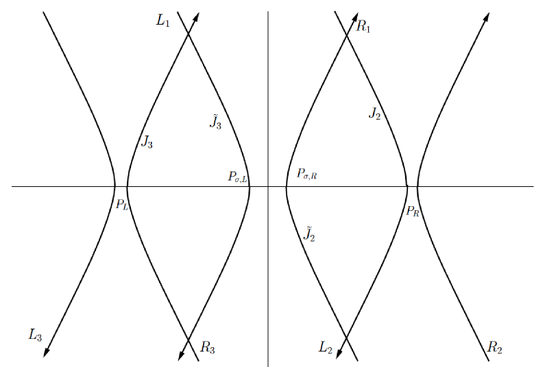
det ( Id − [ A C B − Q L H ~ k + A C B k − H j Q R + A j C B A j C B k ] ) = det [ Id B B k A C Id Q L H ~ k A j C H j Q R Id ] Id delimited-[] 𝐴 𝐶 𝐵 subscript 𝑄 𝐿 subscript ~ 𝐻 𝑘 𝐴 𝐶 subscript 𝐵 𝑘 missing-subexpression missing-subexpression missing-subexpression missing-subexpression subscript 𝐻 𝑗 subscript 𝑄 𝑅 subscript 𝐴 𝑗 𝐶 𝐵 subscript 𝐴 𝑗 𝐶 subscript 𝐵 𝑘 delimited-[] Id 𝐵 subscript 𝐵 𝑘 missing-subexpression missing-subexpression missing-subexpression 𝐴 𝐶 Id subscript 𝑄 𝐿 subscript ~ 𝐻 𝑘 missing-subexpression missing-subexpression missing-subexpression subscript 𝐴 𝑗 𝐶 subscript 𝐻 𝑗 subscript 𝑄 𝑅 Id \displaystyle\det\left(\operatorname{Id}-\left[\begin{array}[]{c|c}ACB&-Q_{L}\widetilde{H}_{k}+ACB_{k}\\
\hline\cr\\
-H_{j}Q_{R}+A_{j}CB&A_{j}CB_{k}\end{array}\right]\right)=\det\left[\begin{array}[]{c|c|c}\operatorname{Id}&B&B_{k}\\
\hline\cr AC&\operatorname{Id}&Q_{L}\widetilde{H}_{k}\\
\hline\cr A_{j}C&H_{j}Q_{R}&\operatorname{Id}\end{array}\right] (3.63)
= det [ Id L 1 0 0 0 0 H ~ k 0 Id R 1 0 0 Q R 0 0 0 Id L 2 C 0 0 0 0 0 Id B B k − Q L 0 − A 0 Id 0 2 0 0 − H j − A j 0 0 Id 0 3 ] = det [ Id L 1 H ~ k H j H ~ k A j 0 Q R Q L Id R 1 Q R A 0 0 0 Id L 2 C B Q L B k H j B A + B k A j Id R 2 ] absent delimited-[] subscript Id subscript 𝐿 1 0 0 0 0 subscript ~ 𝐻 𝑘 missing-subexpression missing-subexpression missing-subexpression missing-subexpression missing-subexpression missing-subexpression 0 subscript Id subscript 𝑅 1 0 0 subscript 𝑄 𝑅 0 missing-subexpression missing-subexpression missing-subexpression missing-subexpression missing-subexpression missing-subexpression 0 0 subscript Id subscript 𝐿 2 𝐶 0 0 missing-subexpression missing-subexpression missing-subexpression missing-subexpression missing-subexpression missing-subexpression 0 0 0 Id 𝐵 subscript 𝐵 𝑘 missing-subexpression missing-subexpression missing-subexpression missing-subexpression missing-subexpression missing-subexpression subscript 𝑄 𝐿 0 𝐴 0 subscript Id subscript 0 2 0 missing-subexpression missing-subexpression missing-subexpression missing-subexpression missing-subexpression missing-subexpression 0 subscript 𝐻 𝑗 subscript 𝐴 𝑗 0 0 subscript Id subscript 0 3 delimited-[] subscript Id subscript 𝐿 1 subscript ~ 𝐻 𝑘 subscript 𝐻 𝑗 subscript ~ 𝐻 𝑘 subscript 𝐴 𝑗 0 missing-subexpression missing-subexpression missing-subexpression missing-subexpression subscript 𝑄 𝑅 subscript 𝑄 𝐿 subscript Id subscript 𝑅 1 subscript 𝑄 𝑅 𝐴 0 missing-subexpression missing-subexpression missing-subexpression missing-subexpression 0 0 subscript Id subscript 𝐿 2 𝐶 missing-subexpression missing-subexpression missing-subexpression missing-subexpression 𝐵 subscript 𝑄 𝐿 subscript 𝐵 𝑘 subscript 𝐻 𝑗 𝐵 𝐴 subscript 𝐵 𝑘 subscript 𝐴 𝑗 subscript Id subscript 𝑅 2 \displaystyle=\det\left[\begin{array}[]{c|c|c|c|c|c}\operatorname{Id}_{L_{1}}&0&0&0&0&\widetilde{H}_{k}\\
\hline\cr 0&\operatorname{Id}_{R_{1}}&0&0&Q_{R}&0\\
\hline\cr 0&0&\operatorname{Id}_{L_{2}}&C&0&0\\
\hline\cr 0&0&0&\operatorname{Id}&B&B_{k}\\
\hline\cr-Q_{L}&0&-A&0&\operatorname{Id}_{0_{2}}&0\\
\hline\cr 0&-H_{j}&-A_{j}&0&0&\operatorname{Id}_{0_{3}}\end{array}\right]=\det\left[\begin{array}[]{c|c|c|c}\operatorname{Id}_{L_{1}}&\widetilde{H}_{k}H_{j}&\widetilde{H}_{k}A_{j}&0\\
\hline\cr Q_{R}Q_{L}&\operatorname{Id}_{R_{1}}&Q_{R}A&0\\
\hline\cr 0&0&\operatorname{Id}_{L_{2}}&C\\
\hline\cr BQ_{L}&B_{k}H_{j}&BA+B_{k}A_{j}&\operatorname{Id}_{R_{2}}\end{array}\right] (3.74)
where by the Id X j subscript Id subscript 𝑋 𝑗 \operatorname{Id}_{X_{j}} L 2 ( X , ℂ ) superscript 𝐿 2 𝑋 ℂ L^{2}(X,{\mathbb{C}})
Proof.
We start by noticing that all operators are Hilbert–Schmidt, and hence the first two determinants and the last one are ordinary Fredholm determinants, since the operators appearing are trace-class; the third determinant should be understood as Carleman regularized det 2 subscript 2 \det_{2} determinant. However, since the operator whose determinant is computed is diagonal-free, the formal definition coincides with the usual Fredholm determinant. The first identity is seen by multiplying on the left by a proper lower triangular matrix, while the second one is given by multiplying the matrix
ℳ = [ Id L 1 0 0 0 0 0 H ~ k 0 Id R 1 0 0 0 Q R 0 0 0 Id L 2 0 C 0 0 0 0 0 Id R 2 0 B B k 0 0 0 0 Id 0 1 0 0 − Q L 0 − A 0 0 Id 0 2 0 0 − H j − A j 0 0 0 Id 0 3 ] ℳ delimited-[] subscript Id subscript 𝐿 1 0 0 0 0 0 subscript ~ 𝐻 𝑘 missing-subexpression missing-subexpression missing-subexpression missing-subexpression missing-subexpression missing-subexpression missing-subexpression 0 subscript Id subscript 𝑅 1 0 0 0 subscript 𝑄 𝑅 0 missing-subexpression missing-subexpression missing-subexpression missing-subexpression missing-subexpression missing-subexpression missing-subexpression 0 0 subscript Id subscript 𝐿 2 0 𝐶 0 0 missing-subexpression missing-subexpression missing-subexpression missing-subexpression missing-subexpression missing-subexpression missing-subexpression 0 0 0 subscript Id subscript 𝑅 2 0 𝐵 subscript 𝐵 𝑘 missing-subexpression missing-subexpression missing-subexpression missing-subexpression missing-subexpression missing-subexpression missing-subexpression 0 0 0 0 subscript Id subscript 0 1 0 0 missing-subexpression missing-subexpression missing-subexpression missing-subexpression missing-subexpression missing-subexpression missing-subexpression subscript 𝑄 𝐿 0 𝐴 0 0 subscript Id subscript 0 2 0 missing-subexpression missing-subexpression missing-subexpression missing-subexpression missing-subexpression missing-subexpression missing-subexpression 0 subscript 𝐻 𝑗 subscript 𝐴 𝑗 0 0 0 subscript Id subscript 0 3 \displaystyle\mathcal{M}=\left[\begin{array}[]{c|c|c|c|c|c|c}\operatorname{Id}_{L_{1}}&0&0&0&0&0&\widetilde{H}_{k}\\
\hline\cr 0&\operatorname{Id}_{R_{1}}&0&0&0&Q_{R}&0\\
\hline\cr 0&0&\operatorname{Id}_{L_{2}}&0&C&0&0\\
\hline\cr 0&0&0&\operatorname{Id}_{R_{2}}&0&B&B_{k}\\
\hline\cr 0&0&0&0&\operatorname{Id}_{0_{1}}&0&0\\
\hline\cr-Q_{L}&0&-A&0&0&\operatorname{Id}_{0_{2}}&0\\
\hline\cr 0&-H_{j}&-A_{j}&0&0&0&\operatorname{Id}_{0_{3}}\end{array}\right] (3.82)
on the left by
𝒩 = [ Id L 1 0 0 0 0 0 0 0 Id R 1 0 0 0 0 0 0 0 Id L 2 0 0 0 0 0 0 0 Id R 2 0 0 0 0 0 0 0 Id 0 1 0 0 Q L 0 A 0 0 Id 0 2 0 0 H j A j 0 0 0 Id 0 3 ] 𝒩 delimited-[] subscript Id subscript 𝐿 1 0 0 0 0 0 0 missing-subexpression missing-subexpression missing-subexpression missing-subexpression missing-subexpression missing-subexpression missing-subexpression 0 subscript Id subscript 𝑅 1 0 0 0 0 0 missing-subexpression missing-subexpression missing-subexpression missing-subexpression missing-subexpression missing-subexpression missing-subexpression 0 0 subscript Id subscript 𝐿 2 0 0 0 0 missing-subexpression missing-subexpression missing-subexpression missing-subexpression missing-subexpression missing-subexpression missing-subexpression 0 0 0 subscript Id subscript 𝑅 2 0 0 0 missing-subexpression missing-subexpression missing-subexpression missing-subexpression missing-subexpression missing-subexpression missing-subexpression 0 0 0 0 subscript Id subscript 0 1 0 0 missing-subexpression missing-subexpression missing-subexpression missing-subexpression missing-subexpression missing-subexpression missing-subexpression subscript 𝑄 𝐿 0 𝐴 0 0 subscript Id subscript 0 2 0 missing-subexpression missing-subexpression missing-subexpression missing-subexpression missing-subexpression missing-subexpression missing-subexpression 0 subscript 𝐻 𝑗 subscript 𝐴 𝑗 0 0 0 subscript Id subscript 0 3 \displaystyle\mathcal{N}=\left[\begin{array}[]{c|c|c|c|c|c|c}\operatorname{Id}_{L_{1}}&0&0&0&0&0&0\\
\hline\cr 0&\operatorname{Id}_{R_{1}}&0&0&0&0&0\\
\hline\cr 0&0&\operatorname{Id}_{L_{2}}&0&0&0&0\\
\hline\cr 0&0&0&\operatorname{Id}_{R_{2}}&0&0&0\\
\hline\cr 0&0&0&0&\operatorname{Id}_{0_{1}}&0&0\\
\hline\cr Q_{L}&0&A&0&0&\operatorname{Id}_{0_{2}}&0\\
\hline\cr 0&H_{j}&A_{j}&0&0&0&\operatorname{Id}_{0_{3}}\end{array}\right] (3.90)
where 0 j subscript 0 𝑗 0_{j} is a copy of the imaginary axis i ℝ 𝑖 ℝ i\mathbb{R} . We now multiply the two matrices in reverse order, as we know that det ( ℳ 𝒩 ) = det ( 𝒩 ℳ ) ℳ 𝒩 𝒩 ℳ \det(\mathcal{M}\mathcal{N})=\det(\mathcal{N}\mathcal{M}) .
In conclusion, we obtain the operator
det [ Id L 1 H ~ k H j H ~ k A j 0 Q R Q L Id R 1 Q R A 0 0 0 Id L 2 C B Q L B k H j B A + B k A j Id R 2 ] delimited-[] subscript Id subscript 𝐿 1 subscript ~ 𝐻 𝑘 subscript 𝐻 𝑗 subscript ~ 𝐻 𝑘 subscript 𝐴 𝑗 0 missing-subexpression missing-subexpression missing-subexpression missing-subexpression subscript 𝑄 𝑅 subscript 𝑄 𝐿 subscript Id subscript 𝑅 1 subscript 𝑄 𝑅 𝐴 0 missing-subexpression missing-subexpression missing-subexpression missing-subexpression 0 0 subscript Id subscript 𝐿 2 𝐶 missing-subexpression missing-subexpression missing-subexpression missing-subexpression 𝐵 subscript 𝑄 𝐿 subscript 𝐵 𝑘 subscript 𝐻 𝑗 𝐵 𝐴 subscript 𝐵 𝑘 subscript 𝐴 𝑗 subscript Id subscript 𝑅 2 \displaystyle\det\left[\begin{array}[]{c|c|c|c}\operatorname{Id}_{L_{1}}&\widetilde{H}_{k}H_{j}&\widetilde{H}_{k}A_{j}&0\\
\hline\cr Q_{R}Q_{L}&\operatorname{Id}_{R_{1}}&Q_{R}A&0\\
\hline\cr 0&0&\operatorname{Id}_{L_{2}}&C\\
\hline\cr BQ_{L}&B_{k}H_{j}&BA+B_{k}A_{j}&\operatorname{Id}_{R_{2}}\end{array}\right] (3.95)
where we have removed the trivial part involving the three copies of i ℝ 𝑖 ℝ i{\mathbb{R}} .
∎
Collecting all the results found so far, we have
Theorem 3.8 .
The gap probability of the tacnode process at single time is
det ( Id − Π 𝕂 ~ Π ) = F 2 ( σ ~ ) − 1 ⋅ det ( Id − 𝕄 ) Id Π ~ 𝕂 Π ⋅ subscript 𝐹 2 superscript ~ 𝜎 1 Id 𝕄 \det(\operatorname{Id}-\Pi\widetilde{\mathbb{K}}\Pi)=F_{2}(\widetilde{\sigma})^{-1}\cdot\det\left(\operatorname{Id}-\mathbb{M}\right) (3.96)
where
𝕄 := [ 0 L 1 − H ~ k H j − H ~ k A j 0 − Q R Q L 0 R 1 − Q R A 0 0 0 0 L 2 − C − B Q L − B k H j − ( B A + B k A j ) 0 R 2 ] assign 𝕄 delimited-[] subscript 0 subscript 𝐿 1 subscript ~ 𝐻 𝑘 subscript 𝐻 𝑗 subscript ~ 𝐻 𝑘 subscript 𝐴 𝑗 0 missing-subexpression missing-subexpression missing-subexpression missing-subexpression subscript 𝑄 𝑅 subscript 𝑄 𝐿 subscript 0 subscript 𝑅 1 subscript 𝑄 𝑅 𝐴 0 missing-subexpression missing-subexpression missing-subexpression missing-subexpression 0 0 subscript 0 subscript 𝐿 2 𝐶 missing-subexpression missing-subexpression missing-subexpression missing-subexpression 𝐵 subscript 𝑄 𝐿 subscript 𝐵 𝑘 subscript 𝐻 𝑗 𝐵 𝐴 subscript 𝐵 𝑘 subscript 𝐴 𝑗 subscript 0 subscript 𝑅 2 \mathbb{M}:=\left[\begin{array}[]{c|c|c|c}0_{L_{1}}&-\widetilde{H}_{k}H_{j}&-\widetilde{H}_{k}A_{j}&0\\
\hline\cr-Q_{R}Q_{L}&0_{R_{1}}&-Q_{R}A&0\\
\hline\cr 0&0&0_{L_{2}}&-C\\
\hline\cr-BQ_{L}&-B_{k}H_{j}&-(BA+B_{k}A_{j})&0_{R_{2}}\end{array}\right] (3.97)
with
Q R Q L ( λ , μ ) = e λ 3 − μ 3 12 2 i π ( λ − μ ) , B Q L ( λ , μ ) = e λ 3 4 − λ σ ~ − μ 3 12 2 i π ( λ − μ ) formulae-sequence subscript 𝑄 𝑅 subscript 𝑄 𝐿 𝜆 𝜇 superscript e superscript 𝜆 3 superscript 𝜇 3 12 2 𝑖 𝜋 𝜆 𝜇 𝐵 subscript 𝑄 𝐿 𝜆 𝜇 superscript e superscript 𝜆 3 4 𝜆 ~ 𝜎 superscript 𝜇 3 12 2 𝑖 𝜋 𝜆 𝜇 \displaystyle Q_{R}Q_{L}(\lambda,\mu)=\frac{{\rm e}^{\frac{\lambda^{3}-\mu^{3}}{12}}}{2i\pi(\lambda-\mu)},\ \ \ \ BQ_{L}(\lambda,\mu)=\frac{{\rm e}^{\frac{\lambda^{3}}{4}-\lambda\widetilde{\sigma}-\frac{\mu^{3}}{12}}}{2i\pi(\lambda-\mu)} (3.98)
Q R A ( λ , μ ) = e μ σ ~ − μ 3 4 + λ 3 12 2 i π ( λ − μ ) , C ( μ , λ ) = e λ 3 − μ 3 12 2 i π ( μ − λ ) formulae-sequence subscript 𝑄 𝑅 𝐴 𝜆 𝜇 superscript e 𝜇 ~ 𝜎 superscript 𝜇 3 4 superscript 𝜆 3 12 2 𝑖 𝜋 𝜆 𝜇 𝐶 𝜇 𝜆 superscript e superscript 𝜆 3 superscript 𝜇 3 12 2 𝑖 𝜋 𝜇 𝜆 \displaystyle Q_{R}A(\lambda,\mu)=\frac{{\rm e}^{\mu\widetilde{\sigma}-\frac{\mu^{3}}{4}+\frac{\lambda^{3}}{12}}}{2i\pi(\lambda-\mu)},\ \ \ \ C(\mu,\lambda)=\frac{{\rm e}^{\frac{\lambda^{3}-\mu^{3}}{12}}}{2i\pi(\mu-\lambda)} (3.99)
H ~ k H j ( μ , λ ) = ∑ j = 1 2 K ( − 1 ) j + 1 h j − 1 ( μ ) h j ( λ ) 2 i π ( μ − λ ) ; h j ( ζ ) := e ζ 3 / 12 + τ 2 2 / 3 ζ 2 − ( a ~ j + σ ~ ) ζ 2 3 formulae-sequence subscript ~ 𝐻 𝑘 subscript 𝐻 𝑗 𝜇 𝜆 superscript subscript 𝑗 1 2 𝐾 superscript 1 𝑗 1 superscript subscript ℎ 𝑗 1 𝜇 subscript ℎ 𝑗 𝜆 2 𝑖 𝜋 𝜇 𝜆 assign subscript ℎ 𝑗 𝜁 superscript e superscript 𝜁 3 12 𝜏 superscript 2 2 3 superscript 𝜁 2 subscript ~ 𝑎 𝑗 ~ 𝜎 𝜁 3 2 \displaystyle\widetilde{H}_{k}H_{j}(\mu,\lambda)=\frac{\sum_{j=1}^{2K}(-1)^{j+1}h_{j}^{-1}(\mu)h_{j}(\lambda)}{2i\pi(\mu-\lambda)}\,;\ \ \ \ h_{j}(\zeta):=\frac{{\rm e}^{\zeta^{3}/12+\frac{\tau}{2^{2/3}}\zeta^{2}-(\tilde{a}_{j}+\widetilde{\sigma})\zeta}}{\sqrt[3]{2}} (3.100)
H ~ k A j ( μ 1 , μ 2 ) = ∑ j = 1 2 K ( − 1 ) j + 1 h j − 1 ( μ 1 ) g j ( μ 2 ) 2 i π ( μ 1 − μ 2 ) ; g j ( ζ ) := e − ζ 3 / 12 + τ 2 2 / 3 ζ 2 − ζ a ~ j 2 3 formulae-sequence subscript ~ 𝐻 𝑘 subscript 𝐴 𝑗 subscript 𝜇 1 subscript 𝜇 2 superscript subscript 𝑗 1 2 𝐾 superscript 1 𝑗 1 superscript subscript ℎ 𝑗 1 subscript 𝜇 1 subscript 𝑔 𝑗 subscript 𝜇 2 2 𝑖 𝜋 subscript 𝜇 1 subscript 𝜇 2 assign subscript 𝑔 𝑗 𝜁 superscript e superscript 𝜁 3 12 𝜏 superscript 2 2 3 superscript 𝜁 2 𝜁 subscript ~ 𝑎 𝑗 3 2 \displaystyle\widetilde{H}_{k}A_{j}(\mu_{1},\mu_{2})=\sum_{j=1}^{2K}(-1)^{j+1}\frac{h_{j}^{-1}(\mu_{1})g_{j}(\mu_{2})}{2i\pi(\mu_{1}-\mu_{2})}\,;\ \ \ \ g_{j}(\zeta):=\frac{{\rm e}^{-\zeta^{3}/12+\frac{\tau}{2^{2/3}}\zeta^{2}-\zeta\tilde{a}_{j}}}{\sqrt[3]{2}} (3.101)
B k H j ( λ 2 , λ 1 ) = ∑ j = 1 2 K ( − 1 ) j g j − 1 ( λ 2 ) h j ( λ 1 ) 2 i π ( λ 2 − λ 1 ) subscript 𝐵 𝑘 subscript 𝐻 𝑗 subscript 𝜆 2 subscript 𝜆 1 superscript subscript 𝑗 1 2 𝐾 superscript 1 𝑗 subscript superscript 𝑔 1 𝑗 subscript 𝜆 2 subscript ℎ 𝑗 subscript 𝜆 1 2 𝑖 𝜋 subscript 𝜆 2 subscript 𝜆 1 \displaystyle B_{k}H_{j}(\lambda_{2},\lambda_{1})=\sum_{j=1}^{2K}(-1)^{j}\frac{g^{-1}_{j}(\lambda_{2})h_{j}(\lambda_{1})}{2i\pi(\lambda_{2}-\lambda_{1})} (3.102)
( B A + B k A j ) ( λ , μ ) = e λ 3 − μ 3 4 + ( μ − λ ) σ ~ 2 i π ( λ − μ ) + ∑ j ( − 1 ) j g j − 1 ( λ ) g j ( μ ) 2 i π ( λ − μ ) 𝐵 𝐴 subscript 𝐵 𝑘 subscript 𝐴 𝑗 𝜆 𝜇 superscript e superscript 𝜆 3 superscript 𝜇 3 4 𝜇 𝜆 ~ 𝜎 2 𝑖 𝜋 𝜆 𝜇 subscript 𝑗 superscript 1 𝑗 superscript subscript 𝑔 𝑗 1 𝜆 subscript 𝑔 𝑗 𝜇 2 𝑖 𝜋 𝜆 𝜇 \displaystyle\left(BA+B_{k}A_{j}\right)(\lambda,\mu)=\frac{{\rm e}^{\frac{\lambda^{3}-\mu^{3}}{4}+(\mu-\lambda)\widetilde{\sigma}}}{2i\pi(\lambda-\mu)}+\sum_{j}(-1)^{j}\frac{g_{j}^{-1}(\lambda)g_{j}(\mu)}{2i\pi(\lambda-\mu)} (3.103)
Proof.
The first three kernels and the kernel B A 𝐵 𝐴 BA follow from easy computations.
Q R Q L ( λ , μ ) = ∫ i ℝ d ζ 2 i π e λ 3 − μ 3 12 2 i π ( λ − ζ ) ( ζ − μ ) = e λ 3 − μ 3 12 2 i π ( λ − μ ) subscript 𝑄 𝑅 subscript 𝑄 𝐿 𝜆 𝜇 subscript 𝑖 ℝ d 𝜁 2 𝑖 𝜋 superscript e superscript 𝜆 3 superscript 𝜇 3 12 2 𝑖 𝜋 𝜆 𝜁 𝜁 𝜇 superscript e superscript 𝜆 3 superscript 𝜇 3 12 2 𝑖 𝜋 𝜆 𝜇 \displaystyle Q_{R}Q_{L}(\lambda,\mu)=\int_{i{\mathbb{R}}}\frac{{\rm d}\zeta}{2i\pi}\frac{{\rm e}^{\frac{\lambda^{3}-\mu^{3}}{12}}}{2i\pi(\lambda-\zeta)(\zeta-\mu)}=\frac{{\rm e}^{\frac{\lambda^{3}-\mu^{3}}{12}}}{2i\pi(\lambda-\mu)} (3.104)
B Q L ( λ , μ ) = ∫ i ℝ d ζ 2 i π e λ 3 4 − λ σ ~ − μ 3 12 2 i π ( λ − ζ ) ( ζ − μ ) = e λ 3 4 − λ σ ~ − μ 3 12 2 i π ( λ − μ ) 𝐵 subscript 𝑄 𝐿 𝜆 𝜇 subscript 𝑖 ℝ d 𝜁 2 𝑖 𝜋 superscript e superscript 𝜆 3 4 𝜆 ~ 𝜎 superscript 𝜇 3 12 2 𝑖 𝜋 𝜆 𝜁 𝜁 𝜇 superscript e superscript 𝜆 3 4 𝜆 ~ 𝜎 superscript 𝜇 3 12 2 𝑖 𝜋 𝜆 𝜇 \displaystyle BQ_{L}(\lambda,\mu)=\int_{i{\mathbb{R}}}\frac{{\rm d}\zeta}{2i\pi}\frac{{\rm e}^{\frac{\lambda^{3}}{4}-\lambda\widetilde{\sigma}-\frac{\mu^{3}}{12}}}{2i\pi(\lambda-\zeta)(\zeta-\mu)}=\frac{{\rm e}^{\frac{\lambda^{3}}{4}-\lambda\widetilde{\sigma}-\frac{\mu^{3}}{12}}}{2i\pi(\lambda-\mu)} (3.105)
Q R A ( λ , μ ) = ∫ i ℝ d ζ 2 i π e μ σ ~ − μ 3 4 + λ 3 12 2 i π ( λ − ζ ) ( ζ − μ ) = e μ σ ~ − μ 3 4 + λ 3 12 2 i π ( λ − μ ) subscript 𝑄 𝑅 𝐴 𝜆 𝜇 subscript 𝑖 ℝ d 𝜁 2 𝑖 𝜋 superscript e 𝜇 ~ 𝜎 superscript 𝜇 3 4 superscript 𝜆 3 12 2 𝑖 𝜋 𝜆 𝜁 𝜁 𝜇 superscript e 𝜇 ~ 𝜎 superscript 𝜇 3 4 superscript 𝜆 3 12 2 𝑖 𝜋 𝜆 𝜇 \displaystyle Q_{R}A(\lambda,\mu)=\int_{i{\mathbb{R}}}\frac{{\rm d}\zeta}{2i\pi}\frac{{\rm e}^{\mu\widetilde{\sigma}-\frac{\mu^{3}}{4}+\frac{\lambda^{3}}{12}}}{2i\pi(\lambda-\zeta)(\zeta-\mu)}=\frac{{\rm e}^{\mu\widetilde{\sigma}-\frac{\mu^{3}}{4}+\frac{\lambda^{3}}{12}}}{2i\pi(\lambda-\mu)} (3.106)
B A ( λ , μ ) = ∫ i ℝ d ζ 2 i π e λ 3 − μ 3 4 + ( μ − λ ) σ ~ 2 i π ( λ − ζ ) ( ζ − μ ) = e λ 3 − μ 3 4 + ( μ − λ ) σ ~ 2 i π ( λ − μ ) 𝐵 𝐴 𝜆 𝜇 subscript 𝑖 ℝ d 𝜁 2 𝑖 𝜋 superscript e superscript 𝜆 3 superscript 𝜇 3 4 𝜇 𝜆 ~ 𝜎 2 𝑖 𝜋 𝜆 𝜁 𝜁 𝜇 superscript e superscript 𝜆 3 superscript 𝜇 3 4 𝜇 𝜆 ~ 𝜎 2 𝑖 𝜋 𝜆 𝜇 \displaystyle BA(\lambda,\mu)=\int_{i{\mathbb{R}}}\frac{{\rm d}\zeta}{2i\pi}\frac{{\rm e}^{\frac{\lambda^{3}-\mu^{3}}{4}+(\mu-\lambda)\widetilde{\sigma}}}{2i\pi(\lambda-\zeta)(\zeta-\mu)}=\frac{{\rm e}^{\frac{\lambda^{3}-\mu^{3}}{4}+(\mu-\lambda)\widetilde{\sigma}}}{2i\pi(\lambda-\mu)} (3.107)
Next, we recall that the endpoints are ordered a ~ j < a ~ j + 1 subscript ~ 𝑎 𝑗 subscript ~ 𝑎 𝑗 1 \tilde{a}_{j}<\tilde{a}_{j+1} , so that we can pick up residues accordingly to the sign of a ~ j − a ~ k subscript ~ 𝑎 𝑗 subscript ~ 𝑎 𝑘 \tilde{a}_{j}-\tilde{a}_{k} ( j , k = 1 , … , 2 K formulae-sequence 𝑗 𝑘
1 … 2 𝐾
j,k=1,\ldots,2K ).
H ~ k H j ( μ , λ ) = ∑ j , k ( − 1 ) j + k + 1 4 3 ∫ i ℝ d ζ 2 i π e ζ ( a ~ j − a ~ k ) e μ a ~ k + μ σ ~ − μ 3 12 − τ 2 2 / 3 μ 2 2 i π ( μ − ζ ) e − λ a ~ j − σ ~ λ + λ 3 12 + τ 2 2 / 3 λ 2 ( ζ − λ ) = subscript ~ 𝐻 𝑘 subscript 𝐻 𝑗 𝜇 𝜆 subscript 𝑗 𝑘
superscript 1 𝑗 𝑘 1 3 4 subscript 𝑖 ℝ d 𝜁 2 𝑖 𝜋 superscript e 𝜁 subscript ~ 𝑎 𝑗 subscript ~ 𝑎 𝑘 superscript e 𝜇 subscript ~ 𝑎 𝑘 𝜇 ~ 𝜎 superscript 𝜇 3 12 𝜏 superscript 2 2 3 superscript 𝜇 2 2 𝑖 𝜋 𝜇 𝜁 superscript e 𝜆 subscript ~ 𝑎 𝑗 ~ 𝜎 𝜆 superscript 𝜆 3 12 𝜏 superscript 2 2 3 superscript 𝜆 2 𝜁 𝜆 absent \displaystyle\widetilde{H}_{k}H_{j}(\mu,\lambda)=\sum_{j,k}\frac{(-1)^{j+k+1}}{\sqrt[3]{4}}\int_{i{\mathbb{R}}}\frac{{\rm d}\zeta}{2i\pi}{\rm e}^{\zeta(\tilde{a}_{j}-\tilde{a}_{k})}\frac{{\rm e}^{\mu\tilde{a}_{k}+\mu\widetilde{\sigma}-\frac{\mu^{3}}{12}-\frac{\tau}{2^{2/3}}\mu^{2}}}{2i\pi(\mu-\zeta)}\frac{{\rm e}^{-\lambda\tilde{a}_{j}-\widetilde{\sigma}\lambda+\frac{\lambda^{3}}{12}+\frac{\tau}{2^{2/3}}\lambda^{2}}}{(\zeta-\lambda)}= (3.108)
∑ j < k ( − 1 ) j + k 4 3 e ( μ − λ ) a ~ k + ( μ − λ ) σ ~ + λ 3 − μ 3 12 + τ 2 2 / 3 ( λ 2 − μ 2 ) 2 i π ( μ − λ ) + ∑ k < j ( − 1 ) j + k 4 3 e ( μ − λ ) a ~ j + ( μ − λ ) σ ~ + λ 3 − μ 3 12 + τ 2 2 / 3 ( λ 2 − μ 2 ) 2 i π ( μ − λ ) + subscript 𝑗 𝑘 superscript 1 𝑗 𝑘 3 4 superscript e 𝜇 𝜆 subscript ~ 𝑎 𝑘 𝜇 𝜆 ~ 𝜎 superscript 𝜆 3 superscript 𝜇 3 12 𝜏 superscript 2 2 3 superscript 𝜆 2 superscript 𝜇 2 2 𝑖 𝜋 𝜇 𝜆 limit-from subscript 𝑘 𝑗 superscript 1 𝑗 𝑘 3 4 superscript e 𝜇 𝜆 subscript ~ 𝑎 𝑗 𝜇 𝜆 ~ 𝜎 superscript 𝜆 3 superscript 𝜇 3 12 𝜏 superscript 2 2 3 superscript 𝜆 2 superscript 𝜇 2 2 𝑖 𝜋 𝜇 𝜆 \displaystyle\sum_{j<k}\frac{(-1)^{j+k}}{\sqrt[3]{4}}\frac{{\rm e}^{(\mu-\lambda)\tilde{a}_{k}+(\mu-\lambda)\widetilde{\sigma}+\frac{\lambda^{3}-\mu^{3}}{12}+\frac{\tau}{2^{2/3}}(\lambda^{2}-\mu^{2})}}{2i\pi(\mu-\lambda)}+\sum_{k<j}\frac{(-1)^{j+k}}{\sqrt[3]{4}}\frac{{\rm e}^{(\mu-\lambda)\tilde{a}_{j}+(\mu-\lambda)\widetilde{\sigma}+\frac{\lambda^{3}-\mu^{3}}{12}+\frac{\tau}{2^{2/3}}(\lambda^{2}-\mu^{2})}}{2i\pi(\mu-\lambda)}+ (3.109)
+ ∑ j = 1 2 K 1 4 3 e ( μ − λ ) a ~ j + ( μ − λ ) σ ~ + λ 3 − μ 3 12 + τ 2 2 / 3 ( λ 2 − μ 2 ) 2 i π ( μ − λ ) superscript subscript 𝑗 1 2 𝐾 1 3 4 superscript e 𝜇 𝜆 subscript ~ 𝑎 𝑗 𝜇 𝜆 ~ 𝜎 superscript 𝜆 3 superscript 𝜇 3 12 𝜏 superscript 2 2 3 superscript 𝜆 2 superscript 𝜇 2 2 𝑖 𝜋 𝜇 𝜆 \displaystyle+\sum_{j=1}^{2K}\frac{1}{\sqrt[3]{4}}\frac{{\rm e}^{(\mu-\lambda)\tilde{a}_{j}+(\mu-\lambda)\widetilde{\sigma}+\frac{\lambda^{3}-\mu^{3}}{12}+\frac{\tau}{2^{2/3}}(\lambda^{2}-\mu^{2})}}{2i\pi(\mu-\lambda)} (3.110)
Thanks to some cancellations, we are left with
H ~ k H j ( μ , λ ) = ∑ j = 1 2 K ( − 1 ) j + 1 4 3 e ( μ − λ ) a ~ j + ( μ − λ ) σ ~ + λ 3 − μ 3 12 + τ 2 2 / 3 ( λ 2 − μ 2 ) 2 i π ( μ − λ ) . subscript ~ 𝐻 𝑘 subscript 𝐻 𝑗 𝜇 𝜆 superscript subscript 𝑗 1 2 𝐾 superscript 1 𝑗 1 3 4 superscript e 𝜇 𝜆 subscript ~ 𝑎 𝑗 𝜇 𝜆 ~ 𝜎 superscript 𝜆 3 superscript 𝜇 3 12 𝜏 superscript 2 2 3 superscript 𝜆 2 superscript 𝜇 2 2 𝑖 𝜋 𝜇 𝜆 \displaystyle\widetilde{H}_{k}H_{j}(\mu,\lambda)=\sum_{j=1}^{2K}\frac{(-1)^{j+1}}{\sqrt[3]{4}}\frac{{\rm e}^{(\mu-\lambda)\tilde{a}_{j}+(\mu-\lambda)\widetilde{\sigma}+\frac{\lambda^{3}-\mu^{3}}{12}+\frac{\tau}{2^{2/3}}(\lambda^{2}-\mu^{2})}}{2i\pi(\mu-\lambda)}. (3.111)
Similarly,
B k A j ( λ , μ ) := ∫ i ℝ d ζ 2 i π ∑ k , j ( − 1 ) k + j e λ 3 12 − τ 2 2 / 3 λ 2 + ( λ − ζ ) a ~ k 2 i π ( λ − ζ ) 4 3 e ( ζ − μ ) a ~ j − μ 3 12 + τ 2 2 / 3 μ 2 ( ζ − μ ) = assign subscript 𝐵 𝑘 subscript 𝐴 𝑗 𝜆 𝜇 subscript 𝑖 ℝ d 𝜁 2 𝑖 𝜋 subscript 𝑘 𝑗
superscript 1 𝑘 𝑗 superscript e superscript 𝜆 3 12 𝜏 superscript 2 2 3 superscript 𝜆 2 𝜆 𝜁 subscript ~ 𝑎 𝑘 2 𝑖 𝜋 𝜆 𝜁 3 4 superscript e 𝜁 𝜇 subscript ~ 𝑎 𝑗 superscript 𝜇 3 12 𝜏 superscript 2 2 3 superscript 𝜇 2 𝜁 𝜇 absent \displaystyle B_{k}A_{j}(\lambda,\mu):=\int_{i{\mathbb{R}}}\frac{{\rm d}\zeta}{2i\pi}\sum_{k,j}\frac{(-1)^{k+j}{\rm e}^{\frac{\lambda^{3}}{12}-\frac{\tau}{2^{2/3}}\lambda^{2}+(\lambda-\zeta)\tilde{a}_{k}}}{2i\pi(\lambda-\zeta)\sqrt[3]{4}}\frac{{\rm e}^{(\zeta-\mu)\tilde{a}_{j}-\frac{\mu^{3}}{12}+\frac{\tau}{2^{2/3}}\mu^{2}}}{(\zeta-\mu)}= (3.112)
= ∑ j = 1 2 K ( − 1 ) j e λ 3 − μ 3 12 − τ 2 2 / 3 ( λ 2 − μ 2 ) + ( λ − μ ) a ~ j 2 i π ( λ − μ ) 4 3 . absent superscript subscript 𝑗 1 2 𝐾 superscript 1 𝑗 superscript e superscript 𝜆 3 superscript 𝜇 3 12 𝜏 superscript 2 2 3 superscript 𝜆 2 superscript 𝜇 2 𝜆 𝜇 subscript ~ 𝑎 𝑗 2 𝑖 𝜋 𝜆 𝜇 3 4 \displaystyle=\sum_{j=1}^{2K}\frac{(-1)^{j}{\rm e}^{\frac{\lambda^{3}-\mu^{3}}{12}-\frac{\tau}{2^{2/3}}(\lambda^{2}-\mu^{2})+(\lambda-\mu)\tilde{a}_{j}}}{2i\pi(\lambda-\mu)\sqrt[3]{4}}. (3.113)
In the next computation, we set λ 1 , λ 2 ∈ γ R subscript 𝜆 1 subscript 𝜆 2
subscript 𝛾 𝑅 \lambda_{1},\lambda_{2}\in\gamma_{R} :
B k H j ( λ 2 , λ 1 ) = ∫ i ℝ d ζ 2 i π ∑ k , j ( − 1 ) k + j e λ 2 3 12 − τ 2 2 / 3 λ 2 2 + ( λ 2 − ζ ) a ~ k 2 i π ( λ 2 − ζ ) 4 3 e ( ζ − λ 1 ) a ~ j − σ ~ λ 1 + λ 1 3 12 + τ 2 2 / 3 λ 1 2 ( ζ − λ 1 ) = subscript 𝐵 𝑘 subscript 𝐻 𝑗 subscript 𝜆 2 subscript 𝜆 1 subscript 𝑖 ℝ d 𝜁 2 𝑖 𝜋 subscript 𝑘 𝑗
superscript 1 𝑘 𝑗 superscript e superscript subscript 𝜆 2 3 12 𝜏 superscript 2 2 3 superscript subscript 𝜆 2 2 subscript 𝜆 2 𝜁 subscript ~ 𝑎 𝑘 2 𝑖 𝜋 subscript 𝜆 2 𝜁 3 4 superscript e 𝜁 subscript 𝜆 1 subscript ~ 𝑎 𝑗 ~ 𝜎 subscript 𝜆 1 superscript subscript 𝜆 1 3 12 𝜏 superscript 2 2 3 superscript subscript 𝜆 1 2 𝜁 subscript 𝜆 1 absent \displaystyle B_{k}H_{j}(\lambda_{2},\lambda_{1})=\int_{i{\mathbb{R}}}\frac{{\rm d}\zeta}{2i\pi}\sum_{k,j}\frac{(-1)^{k+j}{\rm e}^{\frac{\lambda_{2}^{3}}{12}-\frac{\tau}{2^{2/3}}\lambda_{2}^{2}+(\lambda_{2}-\zeta)\tilde{a}_{k}}}{2i\pi(\lambda_{2}-\zeta)\sqrt[3]{4}}\frac{{\rm e}^{(\zeta-\lambda_{1})\tilde{a}_{j}-\widetilde{\sigma}\lambda_{1}+\frac{\lambda_{1}^{3}}{12}+\frac{\tau}{2^{2/3}}\lambda_{1}^{2}}}{(\zeta-\lambda_{1})}= (3.114)
= ∑ j ≤ k ( − 1 ) k + j e λ 2 3 12 − τ 2 2 / 3 λ 2 2 − σ ~ λ 1 + λ 1 3 12 + τ 2 2 / 3 λ 1 2 2 i π ( λ 2 − λ 1 ) 4 3 ( e ( λ 2 − λ 1 ) a ~ j − e ( λ 2 − λ 1 ) a ~ k ) absent subscript 𝑗 𝑘 superscript 1 𝑘 𝑗 superscript e superscript subscript 𝜆 2 3 12 𝜏 superscript 2 2 3 superscript subscript 𝜆 2 2 ~ 𝜎 subscript 𝜆 1 superscript subscript 𝜆 1 3 12 𝜏 superscript 2 2 3 superscript subscript 𝜆 1 2 2 𝑖 𝜋 subscript 𝜆 2 subscript 𝜆 1 3 4 superscript e subscript 𝜆 2 subscript 𝜆 1 subscript ~ 𝑎 𝑗 superscript e subscript 𝜆 2 subscript 𝜆 1 subscript ~ 𝑎 𝑘 \displaystyle=\sum_{j\leq k}\frac{(-1)^{k+j}{\rm e}^{\frac{\lambda_{2}^{3}}{12}-\frac{\tau}{2^{2/3}}\lambda_{2}^{2}-\widetilde{\sigma}\lambda_{1}+\frac{\lambda_{1}^{3}}{12}+\frac{\tau}{2^{2/3}}\lambda_{1}^{2}}}{2i\pi(\lambda_{2}-\lambda_{1})\sqrt[3]{4}}\left({\rm e}^{(\lambda_{2}-\lambda_{1})\tilde{a}_{j}}-{\rm e}^{(\lambda_{2}-\lambda_{1})\tilde{a}_{k}}\right) (3.115)
the first term contributes only with the terms with even j 𝑗 j (with positive sign) , the second only those with odd k 𝑘 k with a negative sign so that
B k H j ( λ 2 , λ 1 ) = ∑ j = 1 2 K ( − 1 ) j e λ 2 3 12 − τ 2 2 / 3 λ 2 2 − σ ~ λ 1 + λ 1 3 12 + τ 2 2 / 3 λ 1 2 2 i π ( λ 2 − λ 1 ) 4 3 e ( λ 2 − λ 1 ) a ~ j subscript 𝐵 𝑘 subscript 𝐻 𝑗 subscript 𝜆 2 subscript 𝜆 1 superscript subscript 𝑗 1 2 𝐾 superscript 1 𝑗 superscript e superscript subscript 𝜆 2 3 12 𝜏 superscript 2 2 3 superscript subscript 𝜆 2 2 ~ 𝜎 subscript 𝜆 1 superscript subscript 𝜆 1 3 12 𝜏 superscript 2 2 3 superscript subscript 𝜆 1 2 2 𝑖 𝜋 subscript 𝜆 2 subscript 𝜆 1 3 4 superscript e subscript 𝜆 2 subscript 𝜆 1 subscript ~ 𝑎 𝑗 \displaystyle B_{k}H_{j}(\lambda_{2},\lambda_{1})=\sum_{j=1}^{2K}\frac{(-1)^{j}{\rm e}^{\frac{\lambda_{2}^{3}}{12}-\frac{\tau}{2^{2/3}}\lambda_{2}^{2}-\widetilde{\sigma}\lambda_{1}+\frac{\lambda_{1}^{3}}{12}+\frac{\tau}{2^{2/3}}\lambda_{1}^{2}}}{2i\pi(\lambda_{2}-\lambda_{1})\sqrt[3]{4}}{\rm e}^{(\lambda_{2}-\lambda_{1})\tilde{a}_{j}} (3.116)
Note that the kernel is regular at λ 1 = λ 2 subscript 𝜆 1 subscript 𝜆 2 \lambda_{1}=\lambda_{2} because the sum vanishes.
In a similar way
H ~ k A j ( μ 1 , μ 2 ) = ∫ i ℝ d ζ 2 i π ∑ k , j ( − 1 ) k + j + 1 e ( μ 1 − ζ ) a ~ k + μ 1 σ ~ − μ 1 3 12 − τ 2 2 / 3 μ 1 2 2 i π ( μ 1 − ζ ) 4 3 e ( ζ − μ 2 ) a ~ j − μ 2 3 12 + τ 2 2 / 3 μ 2 2 ( ζ − μ 2 ) = subscript ~ 𝐻 𝑘 subscript 𝐴 𝑗 subscript 𝜇 1 subscript 𝜇 2 subscript 𝑖 ℝ d 𝜁 2 𝑖 𝜋 subscript 𝑘 𝑗
superscript 1 𝑘 𝑗 1 superscript e subscript 𝜇 1 𝜁 subscript ~ 𝑎 𝑘 subscript 𝜇 1 ~ 𝜎 superscript subscript 𝜇 1 3 12 𝜏 superscript 2 2 3 superscript subscript 𝜇 1 2 2 𝑖 𝜋 subscript 𝜇 1 𝜁 3 4 superscript e 𝜁 subscript 𝜇 2 subscript ~ 𝑎 𝑗 superscript subscript 𝜇 2 3 12 𝜏 superscript 2 2 3 superscript subscript 𝜇 2 2 𝜁 subscript 𝜇 2 absent \displaystyle\widetilde{H}_{k}A_{j}(\mu_{1},\mu_{2})=\int_{i{\mathbb{R}}}\frac{{\rm d}\zeta}{2i\pi}\sum_{k,j}(-1)^{k+j+1}\frac{{\rm e}^{(\mu_{1}-\zeta)\tilde{a}_{k}+\mu_{1}\widetilde{\sigma}-\frac{\mu_{1}^{3}}{12}-\frac{\tau}{2^{2/3}}\mu_{1}^{2}}}{2i\pi(\mu_{1}-\zeta)\sqrt[3]{4}}\frac{{\rm e}^{(\zeta-\mu_{2})\tilde{a}_{j}-\frac{\mu_{2}^{3}}{12}+\frac{\tau}{2^{2/3}}\mu_{2}^{2}}}{(\zeta-\mu_{2})}= (3.117)
= ∑ j ≥ k ( − 1 ) k + j + 1 e μ 1 σ ~ − μ 1 3 12 − τ 2 2 / 3 μ 1 2 2 i π ( μ 1 − μ 2 ) 4 3 e − μ 2 3 12 + τ 2 2 / 3 μ 2 2 1 ( e ( μ 1 − μ 2 ) a ~ k − e ( μ 1 − μ 2 ) a ~ j ) = absent subscript 𝑗 𝑘 superscript 1 𝑘 𝑗 1 superscript e subscript 𝜇 1 ~ 𝜎 superscript subscript 𝜇 1 3 12 𝜏 superscript 2 2 3 superscript subscript 𝜇 1 2 2 𝑖 𝜋 subscript 𝜇 1 subscript 𝜇 2 3 4 superscript e superscript subscript 𝜇 2 3 12 𝜏 superscript 2 2 3 superscript subscript 𝜇 2 2 1 superscript e subscript 𝜇 1 subscript 𝜇 2 subscript ~ 𝑎 𝑘 superscript e subscript 𝜇 1 subscript 𝜇 2 subscript ~ 𝑎 𝑗 absent \displaystyle=\sum_{j\geq k}(-1)^{k+j+1}\frac{{\rm e}^{\mu_{1}\widetilde{\sigma}-\frac{\mu_{1}^{3}}{12}-\frac{\tau}{2^{2/3}}\mu_{1}^{2}}}{2i\pi(\mu_{1}-\mu_{2})\sqrt[3]{4}}\frac{{\rm e}^{-\frac{\mu_{2}^{3}}{12}+\frac{\tau}{2^{2/3}}\mu_{2}^{2}}}{1}\left({\rm e}^{(\mu_{1}-\mu_{2})\tilde{a}_{k}}-{\rm e}^{(\mu_{1}-\mu_{2})\tilde{a}_{j}}\right)= (3.118)
= ∑ j = 1 2 K ( − 1 ) j + 1 e μ 1 σ ~ − μ 1 3 12 − τ 2 2 / 3 μ 1 2 − μ 2 3 12 + τ 2 2 / 3 μ 2 2 2 i π ( μ 1 − μ 2 ) 4 3 e ( μ 2 − μ 1 ) a ~ j absent superscript subscript 𝑗 1 2 𝐾 superscript 1 𝑗 1 superscript e subscript 𝜇 1 ~ 𝜎 superscript subscript 𝜇 1 3 12 𝜏 superscript 2 2 3 superscript subscript 𝜇 1 2 superscript subscript 𝜇 2 3 12 𝜏 superscript 2 2 3 superscript subscript 𝜇 2 2 2 𝑖 𝜋 subscript 𝜇 1 subscript 𝜇 2 3 4 superscript e subscript 𝜇 2 subscript 𝜇 1 subscript ~ 𝑎 𝑗 \displaystyle=\sum_{j=1}^{2K}(-1)^{j+1}\frac{{\rm e}^{\mu_{1}\widetilde{\sigma}-\frac{\mu_{1}^{3}}{12}-\frac{\tau}{2^{2/3}}\mu_{1}^{2}-\frac{\mu_{2}^{3}}{12}+\frac{\tau}{2^{2/3}}\mu_{2}^{2}}}{2i\pi(\mu_{1}-\mu_{2})\sqrt[3]{4}}{\rm e}^{(\mu_{2}-\mu_{1})\tilde{a}_{j}} (3.119)
∎
In conclusion, the kernel can be written as an integrable kernel in the sense of Its-Izergin-Korepin-Slavnov ( [ 16 ] ):
𝕄 ( ξ , ζ ) = f ( ξ ) T ⋅ g ( ζ ) 2 π i ( ξ − ζ ) 𝕄 𝜉 𝜁 ⋅ f superscript 𝜉 𝑇 g 𝜁 2 𝜋 𝑖 𝜉 𝜁 \mathbb{M}(\xi,\zeta)=\frac{\textbf{f}(\xi)^{T}\cdot\textbf{g}(\zeta)}{2\pi i(\xi-\zeta)} (3.120)
with
f ( ξ ) = [ − e − ξ 3 / 12 χ L 2 − e ξ 3 / 4 − ξ σ ~ χ R 2 − e ξ 3 / 12 χ R 1 g 1 − 1 ( ξ ) χ R 2 − h 1 − 1 ( ξ ) χ L 1 ⋮ − ( − 1 ) 2 K g 2 K − 1 ( ξ ) χ R 2 + ( − 1 ) 2 K h 2 K − 1 ( ξ ) χ L 1 ] f 𝜉 delimited-[] superscript e superscript 𝜉 3 12 subscript 𝜒 subscript 𝐿 2 superscript e superscript 𝜉 3 4 𝜉 ~ 𝜎 subscript 𝜒 subscript 𝑅 2 superscript e superscript 𝜉 3 12 subscript 𝜒 subscript 𝑅 1 subscript superscript 𝑔 1 1 𝜉 subscript 𝜒 subscript 𝑅 2 superscript subscript ℎ 1 1 𝜉 subscript 𝜒 subscript 𝐿 1 ⋮ superscript 1 2 𝐾 subscript superscript 𝑔 1 2 𝐾 𝜉 subscript 𝜒 subscript 𝑅 2 superscript 1 2 𝐾 superscript subscript ℎ 2 𝐾 1 𝜉 subscript 𝜒 subscript 𝐿 1 \displaystyle\textbf{f}(\xi)=\left[\begin{array}[]{c}-{\rm e}^{-\xi^{3}/12}\chi_{{}_{L_{2}}}\\[3.0pt]
-{\rm e}^{\xi^{3}/4-\xi\widetilde{\sigma}}\chi_{{}_{R_{2}}}-{\rm e}^{\xi^{3}/12}\chi_{{}_{R_{1}}}\\[3.0pt]
g^{-1}_{1}(\xi)\chi_{{}_{R_{2}}}-h_{1}^{-1}(\xi)\chi_{{}_{L_{1}}}\\[3.0pt]
\vdots\\
-(-1)^{2K}g^{-1}_{{}_{2K}}(\xi)\chi_{{}_{R_{2}}}+(-1)^{2K}h_{{}_{2K}}^{-1}(\xi)\chi_{{}_{L_{1}}}\end{array}\right] (3.126)
g ( ζ ) = [ e ζ 3 / 12 χ R 2 e − ζ 3 / 12 χ L 1 + e − ζ 3 / 4 + ζ σ ~ χ L 2 g 1 ( ζ ) χ L 2 + h 1 ( ζ ) χ R 1 ⋮ g 2 K ( ζ ) χ L 2 + h 2 K ( ζ ) χ R 1 ] g 𝜁 delimited-[] superscript e superscript 𝜁 3 12 subscript 𝜒 subscript 𝑅 2 superscript e superscript 𝜁 3 12 subscript 𝜒 subscript 𝐿 1 superscript e superscript 𝜁 3 4 𝜁 ~ 𝜎 subscript 𝜒 subscript 𝐿 2 subscript 𝑔 1 𝜁 subscript 𝜒 subscript 𝐿 2 subscript ℎ 1 𝜁 subscript 𝜒 subscript 𝑅 1 ⋮ subscript 𝑔 2 𝐾 𝜁 subscript 𝜒 subscript 𝐿 2 subscript ℎ 2 𝐾 𝜁 subscript 𝜒 subscript 𝑅 1 \displaystyle\textbf{g}(\zeta)=\left[\begin{array}[]{c}{\rm e}^{\zeta^{3}/12}\chi_{{}_{R_{2}}}\\[3.0pt]
{\rm e}^{-\zeta^{3}/12}\chi_{{}_{L_{1}}}+{\rm e}^{-\zeta^{3}/4+\zeta\widetilde{\sigma}}\chi_{{}_{L_{2}}}\\[3.0pt]
g_{1}(\zeta)\chi_{{}_{L_{2}}}+h_{1}(\zeta)\chi_{{}_{R_{1}}}\\[3.0pt]
\vdots\\
g_{{}_{2K}}(\zeta)\chi_{{}_{L_{2}}}+h_{{}_{2K}}(\zeta)\chi_{{}_{R_{1}}}\end{array}\right] (3.132)
It is thus natural to associate to it a suitable following RH problem. We refer to [ 15 ] for a detailed explanation.
Proposition 3.9 .
The Fredholm determinant det ( Id − 𝕄 ) Id 𝕄 \det(\mathrm{Id}-\mathbb{M})
Γ + ( λ ) = Γ − ( λ ) J ( λ ) , λ ∈ Σ formulae-sequence subscript Γ 𝜆 subscript Γ 𝜆 𝐽 𝜆 𝜆 Σ \displaystyle\Gamma_{+}(\lambda)=\Gamma_{-}(\lambda)J(\lambda),\quad\lambda\in\Sigma
Γ ( λ ) = I + 𝒪 ( λ − 1 ) , λ → ∞ formulae-sequence Γ 𝜆 𝐼 𝒪 superscript 𝜆 1 → 𝜆 \displaystyle\Gamma(\lambda)=I+\mathcal{O}(\lambda^{-1}),\quad\lambda\rightarrow\infty (3.133)
J ( λ ) := assign 𝐽 𝜆 absent \displaystyle J(\lambda):= (3.134)
[ 1 e − Θ σ ~ χ L e − Θ τ , − a 1 χ L … … e − Θ τ , − a 2 K χ L e Θ σ ~ χ R 1 e Θ − τ , a 1 χ R … … e Θ − τ , a 2 K χ R − e Θ τ , − a 1 χ R e − Θ τ , a 1 χ L 1 … … 0 ⋮ ⋮ 0 … … ⋮ ⋮ ⋮ 0 … … ⋮ ( − 1 ) 2 K e Θ − τ , − a 2 K χ R ( − 1 ) 2 K + 1 e − Θ τ , a 2 K χ L 0 … … 1 ] delimited-[] 1 superscript e subscript Θ ~ 𝜎 subscript 𝜒 𝐿 superscript e subscript Θ 𝜏 subscript 𝑎 1
subscript 𝜒 𝐿 … … superscript e subscript Θ 𝜏 subscript 𝑎 2 𝐾
subscript 𝜒 𝐿 missing-subexpression missing-subexpression missing-subexpression missing-subexpression missing-subexpression missing-subexpression superscript e subscript Θ ~ 𝜎 subscript 𝜒 𝑅 1 superscript e subscript Θ 𝜏 subscript 𝑎 1
subscript 𝜒 𝑅 … … superscript e subscript Θ 𝜏 subscript 𝑎 2 𝐾
subscript 𝜒 𝑅 missing-subexpression missing-subexpression missing-subexpression missing-subexpression missing-subexpression missing-subexpression superscript e subscript Θ 𝜏 subscript 𝑎 1
subscript 𝜒 𝑅 superscript e subscript Θ 𝜏 subscript 𝑎 1
subscript 𝜒 𝐿 1 … … 0 missing-subexpression missing-subexpression missing-subexpression missing-subexpression missing-subexpression missing-subexpression ⋮ ⋮ 0 … … ⋮ missing-subexpression missing-subexpression missing-subexpression missing-subexpression missing-subexpression missing-subexpression ⋮ ⋮ 0 … … ⋮ missing-subexpression missing-subexpression missing-subexpression missing-subexpression missing-subexpression missing-subexpression superscript 1 2 𝐾 superscript e subscript Θ 𝜏 subscript 𝑎 2 𝐾
subscript 𝜒 𝑅 superscript 1 2 𝐾 1 superscript e subscript Θ 𝜏 subscript 𝑎 2 𝐾
subscript 𝜒 𝐿 0 … … 1 \displaystyle\left[\begin{array}[]{c|c|c|c|c|c}1&{\rm e}^{-\Theta_{\widetilde{\sigma}}}\chi_{{}_{L}}&{\rm e}^{-\Theta_{\tau,-a_{1}}}\chi_{{}_{L}}&\ldots&\ldots&{\rm e}^{-\Theta_{\tau,-a_{2K}}}\chi_{{}_{L}}\\
\hline\cr{\rm e}^{\Theta_{\widetilde{\sigma}}}\chi_{{}_{R}}&1&{\rm e}^{\Theta_{-\tau,a_{1}}}\chi_{{}_{R}}&\ldots&\ldots&{\rm e}^{\Theta_{-\tau,a_{2K}}}\chi_{{}_{R}}\\
\hline\cr-{\rm e}^{\Theta_{\tau,-a_{1}}}\chi_{{}_{R}}&{\rm e}^{-\Theta_{\tau,a_{1}}}\chi_{{}_{L}}&1&\ldots&\ldots&0\\
\hline\cr\vdots&\vdots&0&\ldots&\ldots&\vdots\\
\hline\cr\vdots&\vdots&0&\ldots&\ldots&\vdots\\
\hline\cr(-1)^{2K}{\rm e}^{\Theta_{-\tau,-a_{2K}}}\chi_{{}_{R}}&(-1)^{2K+1}{\rm e}^{-\Theta_{\tau,a_{2K}}}\chi_{{}_{L}}&0&\ldots&\ldots&1\end{array}\right] (3.141)
where Σ Σ \Sigma
Θ σ ~ ( λ ) = λ 3 3 − σ ~ λ , Θ τ , a i ( λ ) = λ 3 6 − 2 − 2 3 τ λ 2 − 2 − 1 3 ( a i + σ ) λ . formulae-sequence subscript Θ ~ 𝜎 𝜆 superscript 𝜆 3 3 ~ 𝜎 𝜆 subscript Θ 𝜏 subscript 𝑎 𝑖
𝜆 superscript 𝜆 3 6 superscript 2 2 3 𝜏 superscript 𝜆 2 superscript 2 1 3 subscript 𝑎 𝑖 𝜎 𝜆 \displaystyle\Theta_{\widetilde{\sigma}}(\lambda)=\frac{\lambda^{3}}{3}-\widetilde{\sigma}\lambda,\ \ \ \ \Theta_{\tau,a_{i}}(\lambda)=\frac{\lambda^{3}}{6}-2^{-\frac{2}{3}}\tau\lambda^{2}-2^{-\frac{1}{3}}(a_{i}+\sigma)\lambda. (3.142)
Proof.
It is simply a matter of straightforward calculations: using the standard formula J ( λ ( = I − 2 i π f ( λ ) g ( λ ) T J(\lambda(=I-2i\pi\textbf{f}(\lambda)\textbf{g}(\lambda)^{T} and writing explicitly the endpoints a ~ i subscript ~ 𝑎 𝑖 \tilde{a}_{i} as functions of the original endpoints a i subscript 𝑎 𝑖 a_{i} , we get the jump matrix as in ( 3.134 ), but with two distinct copies of γ R subscript 𝛾 𝑅 \gamma_{R} and γ L subscript 𝛾 𝐿 \gamma_{L} . On the other hand, it is easy to show that the jumps on - say - γ R 1 subscript 𝛾 subscript 𝑅 1 \gamma_{R_{1}} and γ R 2 subscript 𝛾 subscript 𝑅 2 \gamma_{R_{2}} commure, hence we can identify the two contours.
∎
In particular, let’s consider the simplest case where ℐ = [ a , b ] ℐ 𝑎 𝑏 \mathcal{I}=[a,b] , then the RH problem is 4 × 4 4 4 4\times 4 with jump matrix
J ( λ ) = [ 1 e − Θ σ ~ χ L 1 e − Θ τ , − a χ L 2 e − Θ τ , − b χ L 2 e Θ σ ~ χ R 1 1 e Θ − τ , a χ R 3 e Θ − τ , b χ R 3 − e Θ τ , − a χ R 2 e − Θ − τ , a χ L 3 1 0 e Θ τ , − b χ R 2 − e − Θ − τ , b χ L 3 0 1 ] 𝐽 𝜆 delimited-[] 1 superscript 𝑒 subscript Θ ~ 𝜎 subscript 𝜒 subscript 𝐿 1 superscript 𝑒 subscript Θ 𝜏 𝑎
subscript 𝜒 subscript 𝐿 2 superscript 𝑒 subscript Θ 𝜏 𝑏
subscript 𝜒 subscript 𝐿 2 superscript 𝑒 subscript Θ ~ 𝜎 subscript 𝜒 subscript 𝑅 1 1 superscript 𝑒 subscript Θ 𝜏 𝑎
subscript 𝜒 subscript 𝑅 3 superscript 𝑒 subscript Θ 𝜏 𝑏
subscript 𝜒 subscript 𝑅 3 superscript 𝑒 subscript Θ 𝜏 𝑎
subscript 𝜒 subscript 𝑅 2 superscript 𝑒 subscript Θ 𝜏 𝑎
subscript 𝜒 subscript 𝐿 3 1 0 superscript 𝑒 subscript Θ 𝜏 𝑏
subscript 𝜒 subscript 𝑅 2 superscript 𝑒 subscript Θ 𝜏 𝑏
subscript 𝜒 subscript 𝐿 3 0 1 \displaystyle J(\lambda)=\left[\begin{array}[]{cccc}1&e^{-\Theta_{\widetilde{\sigma}}}\chi_{{}_{L_{1}}}&e^{-\Theta_{\tau,-a}}\chi_{{}_{L_{2}}}&e^{-\Theta_{\tau,-b}}\chi_{{}_{L_{2}}}\\
e^{\Theta_{\widetilde{\sigma}}}\chi_{{}_{R_{1}}}&1&e^{\Theta_{-\tau,a}}\chi_{{}_{R_{3}}}&e^{\Theta_{-\tau,b}}\chi_{{}_{R_{3}}}\\
-e^{\Theta_{\tau,-a}}\chi_{{}_{R_{2}}}&e^{-\Theta_{-\tau,a}}\chi_{{}_{L_{3}}}&1&0\\
e^{\Theta_{\tau,-b}}\chi_{{}_{R_{2}}}&-e^{-\Theta_{-\tau,b}}\chi_{{}_{L_{3}}}&0&1\end{array}\right] (3.147)
where
Θ σ ~ ( λ ) = λ 3 3 − σ ~ λ , Θ τ , a i ( λ ) = λ 3 6 − 2 − 2 3 τ λ 2 − 2 − 1 3 ( a i + σ ) λ . formulae-sequence subscript Θ ~ 𝜎 𝜆 superscript 𝜆 3 3 ~ 𝜎 𝜆 subscript Θ 𝜏 subscript 𝑎 𝑖
𝜆 superscript 𝜆 3 6 superscript 2 2 3 𝜏 superscript 𝜆 2 superscript 2 1 3 subscript 𝑎 𝑖 𝜎 𝜆 \displaystyle\Theta_{\widetilde{\sigma}}(\lambda)=\frac{\lambda^{3}}{3}-\widetilde{\sigma}\lambda,\ \ \ \ \Theta_{\tau,a_{i}}(\lambda)=\frac{\lambda^{3}}{6}-2^{-\frac{2}{3}}\tau\lambda^{2}-2^{-\frac{1}{3}}(a_{i}+\sigma)\lambda. (3.148)
(we have renamed the contours R 1 , R 2 , R 3 subscript 𝑅 1 subscript 𝑅 2 subscript 𝑅 3
R_{1},R_{2},R_{3} and L 1 , L 2 , L 3 subscript 𝐿 1 subscript 𝐿 2 subscript 𝐿 3
L_{1},L_{2},L_{3} ).
We will now focus exclusively on the single-interval case and we will apply a steepest descent method in order to prove the factorization of the gap probability of Tacnode process into two gap probabilities of the Airy process. The starting point is the 4 × 4 4 4 4\times 4 Riemann-Hilbert problem ( 3.147 ) with contour configuration as in Figure 3 or Figure 5 , depending on the scaling regime we are considering.
4 Proof of Theorem 2.2
From now on, we are assuming τ > 0 𝜏 0 \tau>0 . For τ ≤ 0 𝜏 0 \tau\leq 0 the calculations follow the same guidelines as below.
The phase functions Θ τ ( λ , − b ) subscript Θ 𝜏 𝜆 𝑏 \Theta_{\tau}(\lambda,-b) and Θ − τ ( λ , a ) subscript Θ 𝜏 𝜆 𝑎 \Theta_{-\tau}(\lambda,a) (appearing in the entries of the 2 × 2 2 2 2\times 2 off-diagonal blocks of the jump matrix ( 3.147 )) have inflection points with zero derivative when the discriminant of the derivative vanishes, which occurs when
a crit + σ + τ 2 = 0 subscript 𝑎 crit 𝜎 superscript 𝜏 2 0 \displaystyle a_{\rm crit}+\sigma+\tau^{2}=0 (4.1)
b crit − σ − τ 2 = 0 subscript 𝑏 crit 𝜎 superscript 𝜏 2 0 \displaystyle b_{\rm crit}-\sigma-\tau^{2}=0 (4.2)
with critical values Θ τ ( λ , − b crit ) = 2 1 / 3 τ subscript Θ 𝜏 𝜆 subscript 𝑏 crit superscript 2 1 3 𝜏 \Theta_{\tau}(\lambda,-b_{\rm crit})=2^{1/3}\tau and Θ − τ ( λ , a crit ) = − 2 1 / 3 τ subscript Θ 𝜏 𝜆 subscript 𝑎 crit superscript 2 1 3 𝜏 \Theta_{-\tau}(\lambda,a_{\rm crit})=-2^{1/3}\tau . The neighbourhood of the discriminant is parametrizable as follows
a = a ( t ) = − σ − τ 2 + t 𝑎 𝑎 𝑡 𝜎 superscript 𝜏 2 𝑡 \displaystyle a=a(t)=-\sigma-\tau^{2}+t (4.3)
b = b ( s ) = σ + τ 2 − s 𝑏 𝑏 𝑠 𝜎 superscript 𝜏 2 𝑠 \displaystyle b=b(s)=\sigma+\tau^{2}-s (4.4)
Thus we have the expressions
Θ τ ( λ , − b ) = ξ − 3 3 − s ξ − + τ 3 3 − s τ , ξ − := λ − 2 1 3 τ 2 1 3 formulae-sequence subscript Θ 𝜏 𝜆 𝑏 superscript subscript 𝜉 3 3 𝑠 subscript 𝜉 superscript 𝜏 3 3 𝑠 𝜏 assign subscript 𝜉 𝜆 superscript 2 1 3 𝜏 superscript 2 1 3 \displaystyle\Theta_{\tau}(\lambda,-b)=\frac{\xi_{-}^{3}}{3}-s\xi_{-}+\frac{\tau^{3}}{3}-s\tau,\ \ \ \xi_{-}:=\frac{\lambda-2^{\frac{1}{3}}\tau}{2^{\frac{1}{3}}} (4.5)
Θ − τ ( λ , a ) = ξ + 3 3 − t ξ + − τ 3 3 + t τ , ξ + := λ + 2 1 3 τ 2 1 3 formulae-sequence subscript Θ 𝜏 𝜆 𝑎 superscript subscript 𝜉 3 3 𝑡 subscript 𝜉 superscript 𝜏 3 3 𝑡 𝜏 assign subscript 𝜉 𝜆 superscript 2 1 3 𝜏 superscript 2 1 3 \displaystyle\Theta_{-\tau}(\lambda,a)=\frac{\xi_{+}^{3}}{3}-t\xi_{+}-\frac{\tau^{3}}{3}+t\tau,\ \ \ \xi_{+}:=\frac{\lambda+2^{\frac{1}{3}}\tau}{2^{\frac{1}{3}}} (4.6)
On the other hand, the phase Θ σ ~ subscript Θ ~ 𝜎 \Theta_{\widetilde{\sigma}} in the entries ( 1 , 2 ) 1 2 (1,2) and ( 2 , 1 ) 2 1 (2,1) of ( 3.147 ) has critical point at ± σ ~ = ± 2 2 3 σ plus-or-minus ~ 𝜎 plus-or-minus superscript 2 2 3 𝜎 \pm\sqrt{\widetilde{\sigma}}=\pm\sqrt{2^{\frac{2}{3}}\sigma} .
Preliminary step.
We conjugate the matrix Γ Γ \Gamma by the constant (with respect to λ 𝜆 \lambda ) diagonal matrix
D := diag ( 1 , 1 , − K ( t ) , − K ( s ) ) assign 𝐷 diag 1 1 𝐾 𝑡 𝐾 𝑠 D:=\operatorname{diag}(1,1,-K(t),-K(s)) (4.7)
where K ( u ) := τ 3 3 − u τ assign 𝐾 𝑢 superscript 𝜏 3 3 𝑢 𝜏 K(u):=\frac{\tau^{3}}{3}-u\tau . As a result, also the jump matrices ( 3.147 ) are similarly conjugated and this has the effect of replacing the phases Θ ± τ , ∓ a subscript Θ plus-or-minus 𝜏 minus-or-plus 𝑎
\Theta_{\pm\tau,\mp a} and Θ ± τ , ∓ b subscript Θ plus-or-minus 𝜏 minus-or-plus 𝑏
\Theta_{\pm\tau,\mp b} by “ Θ ± τ , ∓ a ∓ K ( t ) minus-or-plus subscript Θ plus-or-minus 𝜏 minus-or-plus 𝑎
𝐾 𝑡 \Theta_{\pm\tau,\mp a}\mp K(t) ” and “ Θ ± τ , ∓ b ∓ K ( s ) minus-or-plus subscript Θ plus-or-minus 𝜏 minus-or-plus 𝑏
𝐾 𝑠 \Theta_{\pm\tau,\mp b}\mp K(s) ” respectively, so that their critical value is zero.
We denote by a hat the new matrix and respective jump
Γ ^ := e − D Γ e D J ^ := e − D J e D formulae-sequence assign ^ Γ superscript 𝑒 𝐷 Γ superscript 𝑒 𝐷 assign ^ 𝐽 superscript 𝑒 𝐷 𝐽 superscript 𝑒 𝐷 \hat{\Gamma}:=e^{-D}\Gamma e^{D}\ \ \ \hat{J}:=e^{-D}Je^{D} (4.8)
Thus, the resulting jump J ^ ^ 𝐽 \hat{J} has the following form:
[ 1 e − Θ σ ~ 0 0 0 1 0 0 0 0 1 0 0 0 0 1 ] on L 1 , [ 1 0 0 0 e Θ σ ~ 1 0 0 0 0 1 0 0 0 0 1 ] on R 1 , delimited-[] 1 superscript 𝑒 subscript Θ ~ 𝜎 0 0 0 1 0 0 0 0 1 0 0 0 0 1 on subscript 𝐿 1 delimited-[] 1 0 0 0 superscript 𝑒 subscript Θ ~ 𝜎 1 0 0 0 0 1 0 0 0 0 1 on subscript 𝑅 1
\displaystyle\left[\begin{array}[]{cccc}1&e^{-\Theta_{\widetilde{\sigma}}}&0&0\\
0&1&0&0\\
0&0&1&0\\
0&0&0&1\end{array}\right]\ \ \text{on}\ L_{1},\ \ \ \left[\begin{array}[]{cccc}1&0&0&0\\
e^{\Theta_{\widetilde{\sigma}}}&1&0&0\\
0&0&1&0\\
0&0&0&1\end{array}\right]\ \ \text{on}\ R_{1}, (4.17)
[ 1 0 e − Θ τ , − a + K ( t ) e − Θ ( ξ − , s ) 0 1 0 0 0 0 1 0 0 0 0 1 ] on L 2 , [ 1 0 0 0 0 1 0 0 − e Θ τ , − a − K ( t ) 0 1 0 e Θ ( ξ − , s ) 0 0 1 ] on R 2 , delimited-[] 1 0 superscript 𝑒 subscript Θ 𝜏 𝑎
𝐾 𝑡 superscript 𝑒 Θ subscript 𝜉 𝑠 0 1 0 0 0 0 1 0 0 0 0 1 on subscript 𝐿 2 delimited-[] 1 0 0 0 0 1 0 0 superscript 𝑒 subscript Θ 𝜏 𝑎
𝐾 𝑡 0 1 0 superscript 𝑒 Θ subscript 𝜉 𝑠 0 0 1 on subscript 𝑅 2
\displaystyle\left[\begin{array}[]{cccc}1&0&e^{-\Theta_{\tau,-a}+K(t)}&e^{-\Theta(\xi_{-},s)}\\
0&1&0&0\\
0&0&1&0\\
0&0&0&1\end{array}\right]\ \ \text{on}\ L_{2},\ \ \ \left[\begin{array}[]{cccc}1&0&0&0\\
0&1&0&0\\
-e^{\Theta_{\tau,-a}-K(t)}&0&1&0\\
e^{\Theta(\xi_{-},s)}&0&0&1\end{array}\right]\ \ \text{on}\ R_{2}, (4.26)
[ 1 0 0 0 0 1 0 0 0 e − Θ ( ξ + , t ) 1 0 0 − e − Θ − τ , b − K ( s ) 0 1 ] on L 3 , [ 1 0 0 0 0 1 e Θ ( ξ + , t ) e Θ − τ , b + K ( s ) 0 0 1 0 0 0 0 1 ] on R 3 , delimited-[] 1 0 0 0 0 1 0 0 0 superscript 𝑒 Θ subscript 𝜉 𝑡 1 0 0 superscript 𝑒 subscript Θ 𝜏 𝑏
𝐾 𝑠 0 1 on subscript 𝐿 3 delimited-[] 1 0 0 0 0 1 superscript 𝑒 Θ subscript 𝜉 𝑡 superscript 𝑒 subscript Θ 𝜏 𝑏
𝐾 𝑠 0 0 1 0 0 0 0 1 on subscript 𝑅 3
\displaystyle\left[\begin{array}[]{cccc}1&0&0&0\\
0&1&0&0\\
0&e^{-\Theta(\xi_{+},t)}&1&0\\
0&-e^{-\Theta_{-\tau,b}-K(s)}&0&1\end{array}\right]\ \ \text{on}\ L_{3},\ \ \ \left[\begin{array}[]{cccc}1&0&0&0\\
0&1&e^{\Theta(\xi_{+},t)}&e^{\Theta_{-\tau,b}+K(s)}\\
0&0&1&0\\
0&0&0&1\end{array}\right]\ \ \text{on}\ R_{3}, (4.35)
where
Θ ( ξ ± , u ) := ξ ± 3 3 − ξ ± u ξ ± := λ ± 2 3 τ 2 3 formulae-sequence assign Θ subscript 𝜉 plus-or-minus 𝑢 superscript subscript 𝜉 plus-or-minus 3 3 subscript 𝜉 plus-or-minus 𝑢 assign subscript 𝜉 plus-or-minus plus-or-minus 𝜆 3 2 𝜏 3 2 \displaystyle\Theta(\xi_{\pm},u):=\frac{\xi_{\pm}^{3}}{3}-\xi_{\pm}u\ \ \ \ \ \xi_{\pm}:=\frac{\lambda\pm\sqrt[3]{2}\tau}{\sqrt[3]{2}} (4.36)
Θ − τ , b ( λ , s ) := λ 3 6 + τ λ 2 2 2 / 3 − 2 2 / 3 σ λ − τ 2 λ 2 3 + s λ 2 3 assign subscript Θ 𝜏 𝑏
𝜆 𝑠 superscript 𝜆 3 6 𝜏 superscript 𝜆 2 superscript 2 2 3 superscript 2 2 3 𝜎 𝜆 superscript 𝜏 2 𝜆 3 2 𝑠 𝜆 3 2 \displaystyle\Theta_{-\tau,b}(\lambda,s):=\frac{\lambda^{3}}{6}+\frac{\tau\lambda^{2}}{2^{2/3}}-2^{2/3}\sigma\lambda-\frac{\tau^{2}\lambda}{\sqrt[3]{2}}+\frac{s\lambda}{\sqrt[3]{2}} (4.37)
Θ τ , − a ( λ , t ) := λ 3 6 − τ λ 2 2 2 / 3 − 2 2 / 3 σ λ − τ 2 λ 2 3 + t λ 2 3 assign subscript Θ 𝜏 𝑎
𝜆 𝑡 superscript 𝜆 3 6 𝜏 superscript 𝜆 2 superscript 2 2 3 superscript 2 2 3 𝜎 𝜆 superscript 𝜏 2 𝜆 3 2 𝑡 𝜆 3 2 \displaystyle\Theta_{\tau,-a}(\lambda,t):=\frac{\lambda^{3}}{6}-\frac{\tau\lambda^{2}}{2^{2/3}}-2^{2/3}\sigma\lambda-\frac{\tau^{2}\lambda}{\sqrt[3]{2}}+\frac{t\lambda}{\sqrt[3]{2}} (4.38)
We choose the contours according to the following configuration (see Figure 3 ):
•
L 2 subscript 𝐿 2 L_{2} and R 2 subscript 𝑅 2 R_{2} are centred around the critical point P R := 2 1 3 τ assign subscript 𝑃 𝑅 superscript 2 1 3 𝜏 P_{R}:=2^{\frac{1}{3}}\tau
•
L 3 subscript 𝐿 3 L_{3} and R 3 subscript 𝑅 3 R_{3} are centred around the critical point P L := − 2 1 3 τ assign subscript 𝑃 𝐿 superscript 2 1 3 𝜏 P_{L}:=-2^{\frac{1}{3}}\tau
•
L 1 subscript 𝐿 1 L_{1} passes through the critical point P σ , L := − σ ~ assign subscript 𝑃 𝜎 𝐿
~ 𝜎 P_{\sigma,L}:=-\sqrt{\widetilde{\sigma}} and R 1 subscript 𝑅 1 R_{1} passes through the critical point P σ , R := σ ~ assign subscript 𝑃 𝜎 𝑅
~ 𝜎 P_{\sigma,R}:=\sqrt{\widetilde{\sigma}} ; these points are thought as very far from the origin, in the limit as σ ≫ 1 much-greater-than 𝜎 1 \sigma\gg 1 .
Figure 3: The contour setting in the asymptotic limit as σ → + ∞ → 𝜎 \sigma\rightarrow+\infty
Remark 4.1 .
All the left jumps commute with themselves and similarly all the right jumps. Moreover, the jump matrices L 2 subscript 𝐿 2 L_{2} R 3 subscript 𝑅 3 R_{3}
The proof now proceeds along the following scheme (as σ → + ∞ → 𝜎 \sigma\rightarrow+\infty ):
1.
the matrices L 1 subscript 𝐿 1 L_{1} and R 1 subscript 𝑅 1 R_{1} are exponentially close to the identity in every L p superscript 𝐿 𝑝 L^{p} norm (Lemma 4.2 );
2.
regarding the matrices L 2 subscript 𝐿 2 L_{2} and R 2 subscript 𝑅 2 R_{2} , the entries of the form ± ( Θ τ , − a − K ( t ) ) plus-or-minus subscript Θ 𝜏 𝑎
𝐾 𝑡 \pm(\Theta_{\tau,-a}-K(t)) are exponentially small in every L p superscript 𝐿 𝑝 L^{p} norm; the same behaviour will appear for the entries of the type ± ( Θ − τ , b + K ( s ) ) plus-or-minus subscript Θ 𝜏 𝑏
𝐾 𝑠 \pm(\Theta_{-\tau,b}+K(s)) in the matrices L 3 subscript 𝐿 3 L_{3} and R 3 subscript 𝑅 3 R_{3} (Lemma 4.3 );
3.
for the remaining entries in the jumps L 2 , 3 subscript 𝐿 2 3
L_{2,3} and R 2 , 3 subscript 𝑅 2 3
R_{2,3} we will explicitly and exactly solve a (model) Riemann-Hilbert problem which will approximate the problem at hand.
4.1 Estimates on the phases
The proof of the first two points rely on the following lemmas.
Lemma 4.2 .
The jumps on the curves L 1 subscript 𝐿 1 L_{1} R 1 subscript 𝑅 1 R_{1} L p superscript 𝐿 𝑝 L^{p} 1 ≤ p ≤ ∞ 1 𝑝 1\leq p\leq\infty σ → + ∞ → 𝜎 \sigma\rightarrow+\infty
Proof.
A parametrization for the curves L 1 subscript 𝐿 1 L_{1} and R 1 subscript 𝑅 1 R_{1} is the following λ = ± 2 1 / 3 σ + u ( 1 2 ± 3 2 i ) 𝜆 plus-or-minus superscript 2 1 3 𝜎 𝑢 plus-or-minus 1 2 3 2 𝑖 \lambda=\pm 2^{1/3}\sqrt{\sigma}+u\left(\frac{1}{2}\pm\frac{\sqrt{3}}{2}i\right) .
Therefore, we have (for both signs)
ℜ [ Θ σ ~ ; R 1 ] = ℜ [ − Θ σ ~ ; L 1 ] = − 4 3 σ 3 / 2 − σ 2 2 / 3 u 2 − u 3 3 subscript Θ ~ 𝜎 subscript 𝑅 1
subscript Θ ~ 𝜎 subscript 𝐿 1
4 3 superscript 𝜎 3 2 𝜎 superscript 2 2 3 superscript 𝑢 2 superscript 𝑢 3 3 \displaystyle\Re\left[\Theta_{\tilde{\sigma};R_{1}}\right]=\Re\left[-\Theta_{\tilde{\sigma};L_{1}}\right]=-\frac{4}{3}\sigma^{3/2}-\frac{\sqrt{\sigma}}{2^{2/3}}u^{2}-\frac{u^{3}}{3} (4.39)
which implies
‖ e Θ σ ~ ‖ L p ( R 1 ) p = 2 ∫ 0 ∞ e p ℜ [ Θ σ ~ ] 𝑑 u ≤ C e − 4 3 p σ 3 / 2 , ‖ e Θ σ ~ ‖ L ∞ ( R 1 ) = e − 4 3 σ 3 / 2 formulae-sequence subscript superscript norm superscript 𝑒 subscript Θ ~ 𝜎 𝑝 superscript 𝐿 𝑝 subscript 𝑅 1 2 superscript subscript 0 superscript 𝑒 𝑝 subscript Θ ~ 𝜎 differential-d 𝑢 𝐶 superscript 𝑒 4 3 𝑝 superscript 𝜎 3 2 subscript norm superscript 𝑒 subscript Θ ~ 𝜎 superscript 𝐿 subscript 𝑅 1 superscript 𝑒 4 3 superscript 𝜎 3 2 \displaystyle\left\|e^{\Theta_{\tilde{\sigma}}}\right\|^{p}_{L^{p}(R_{1})}=2\int_{0}^{\infty}e^{p\Re\left[\Theta_{\tilde{\sigma}}\right]}du\leq Ce^{-\frac{4}{3}p\sigma^{3/2}},\ \ \left\|e^{\Theta_{\tilde{\sigma}}}\right\|_{L^{\infty}(R_{1})}=e^{-\frac{4}{3}\sigma^{3/2}} (4.40)
The same results holds for the contour L 1 subscript 𝐿 1 L_{1} .
∎
Lemma 4.3 .
Given 0 < K 1 < 1 0 subscript 𝐾 1 1 0<K_{1}<1 s < K 1 ( σ + τ 2 ) 𝑠 subscript 𝐾 1 𝜎 superscript 𝜏 2 s<K_{1}(\sigma+\tau^{2}) e Θ ( − τ , b ) + K ( s ) superscript 𝑒 Θ 𝜏 𝑏 𝐾 𝑠 e^{\Theta(-\tau,b)+K(s)} L p ( R 3 ) superscript 𝐿 𝑝 subscript 𝑅 3 L^{p}(R_{3}) 1 ≤ p ≤ ∞ 1 𝑝 1\leq p\leq\infty σ → + ∞ → 𝜎 \sigma\rightarrow+\infty
‖ e Θ ( − τ , b ) + K ( s ) ‖ L p ( R 3 ) ≤ C e − 2 τ ( 1 − K 1 ) σ subscript norm superscript 𝑒 Θ 𝜏 𝑏 𝐾 𝑠 superscript 𝐿 𝑝 subscript 𝑅 3 𝐶 superscript 𝑒 2 𝜏 1 subscript 𝐾 1 𝜎 \left\|e^{\Theta(-\tau,b)+K(s)}\right\|_{L^{p}(R_{3})}\leq Ce^{-2\tau(1-K_{1})\sigma} (4.41)
Similarly, the function e − Θ ( − τ , b ) − K ( s ) superscript 𝑒 Θ 𝜏 𝑏 𝐾 𝑠 e^{-\Theta(-\tau,b)-K(s)} L p ( L 3 ) superscript 𝐿 𝑝 subscript 𝐿 3 L^{p}(L_{3}) 1 ≤ p ≤ ∞ 1 𝑝 1\leq p\leq\infty
Moreover, the function e − Θ τ , − a + K ( t ) superscript 𝑒 subscript Θ 𝜏 𝑎
𝐾 𝑡 e^{-\Theta_{\tau,-a}+K(t)} e Θ τ , − a − K ( t ) superscript 𝑒 subscript Θ 𝜏 𝑎
𝐾 𝑡 e^{\Theta_{\tau,-a}-K(t)} L p ( L 2 ) superscript 𝐿 𝑝 subscript 𝐿 2 L^{p}(L_{2}) L p ( R 2 ) superscript 𝐿 𝑝 subscript 𝑅 2 L^{p}(R_{2}) 1 ≤ p ≤ ∞ 1 𝑝 1\leq p\leq\infty
Proof.
A parametrization of R 3 subscript 𝑅 3 R_{3} is λ = 2 3 τ + u [ 1 2 ± 2 3 i ] 𝜆 3 2 𝜏 𝑢 delimited-[] plus-or-minus 1 2 2 3 𝑖 \lambda=\sqrt[3]{2}\tau+u\left[\frac{1}{2}\pm\frac{2}{\sqrt{3}}i\right] , u ≥ 0 𝑢 0 u\geq 0 . This yields
ℜ [ Θ ( − τ , b ) + K ( s ) ] = − u 3 6 − δ u 2 4 3 − 2 τ σ − 2 τ 3 + 2 τ δ Θ 𝜏 𝑏 𝐾 𝑠 superscript 𝑢 3 6 𝛿 𝑢 superscript 2 4 3 2 𝜏 𝜎 2 superscript 𝜏 3 2 𝜏 𝛿 \displaystyle\Re\left[\Theta(-\tau,b)+K(s)\right]=-\frac{u^{3}}{6}-\frac{\delta u}{2^{\frac{4}{3}}}-2\tau\sigma-2{\tau}^{3}+2\tau\delta (4.42)
where we set s = 2 σ + 2 τ 2 − δ 𝑠 2 𝜎 2 superscript 𝜏 2 𝛿 s=2\sigma+2\tau^{2}-\delta , 0 < δ < σ + τ 2 0 𝛿 𝜎 superscript 𝜏 2 0<\delta<\sigma+\tau^{2} , and this is valid for both branches of the curve.
Regarding the L p ( R 3 ) superscript 𝐿 𝑝 subscript 𝑅 3 L^{p}(R_{3}) norms, we have that | e Θ − τ , b + K ( s ) | = e ℜ [ Θ − τ , b + K ( s ) ] superscript 𝑒 subscript Θ 𝜏 𝑏
𝐾 𝑠 superscript 𝑒 subscript Θ 𝜏 𝑏
𝐾 𝑠 \left|e^{\Theta_{-\tau,b}+K(s)}\right|=e^{\Re[\Theta_{-\tau,b}+K(s)]} ; therefore,
‖ e Θ ( − τ , b ) + K ( s ) ‖ L p ( R 3 ) p ≤ 2 C e − 2 p τ ( σ + τ 2 − δ ) [ ∫ 0 1 e − 2 − 4 3 p δ u 𝑑 u + ∫ 1 ∞ e − p u 3 6 𝑑 u ] subscript superscript norm superscript 𝑒 Θ 𝜏 𝑏 𝐾 𝑠 𝑝 superscript 𝐿 𝑝 subscript 𝑅 3 2 𝐶 superscript 𝑒 2 𝑝 𝜏 𝜎 superscript 𝜏 2 𝛿 delimited-[] superscript subscript 0 1 superscript 𝑒 superscript 2 4 3 𝑝 𝛿 𝑢 differential-d 𝑢 superscript subscript 1 superscript 𝑒 𝑝 superscript 𝑢 3 6 differential-d 𝑢 \displaystyle\left\|e^{\Theta(-\tau,b)+K(s)}\right\|^{p}_{L^{p}(R_{3})}\leq 2Ce^{-2p\tau(\sigma+\tau^{2}-\delta)}\left[\int_{0}^{1}e^{-2^{-\frac{4}{3}}p\delta u}du+\int_{1}^{\infty}e^{-p\frac{u^{3}}{6}}du\right]
≤ C e − 2 p τ ( 1 − K 1 ) σ absent 𝐶 superscript 𝑒 2 𝑝 𝜏 1 subscript 𝐾 1 𝜎 \displaystyle\leq Ce^{-2p\tau(1-K_{1})\sigma} (4.43)
‖ e Θ ( − τ , b ) + K ( s ) ‖ L ∞ ( R 3 ) = e − 2 τ ( σ + τ 2 − δ ) ≤ C e − 2 τ ( 1 − K 1 ) σ subscript norm superscript 𝑒 Θ 𝜏 𝑏 𝐾 𝑠 superscript 𝐿 subscript 𝑅 3 superscript 𝑒 2 𝜏 𝜎 superscript 𝜏 2 𝛿 𝐶 superscript 𝑒 2 𝜏 1 subscript 𝐾 1 𝜎 \displaystyle\left\|e^{\Theta(-\tau,b)+K(s)}\right\|_{L^{\infty}(R_{3})}=e^{-2\tau(\sigma+\tau^{2}-\delta)}\leq Ce^{-2\tau(1-K_{1})\sigma} (4.44)
given that s < K 1 ( σ + τ 2 ) 𝑠 subscript 𝐾 1 𝜎 superscript 𝜏 2 s<K_{1}(\sigma+\tau^{2}) with 0 < K 1 < 1 0 subscript 𝐾 1 1 0<K_{1}<1 .
All the other cases are completely analogous.
∎
4.2 Global parametrix. The model problem
In this subsection we will use the Hasting-McLeod matrix (see [ 12 ] , but in the normalization of [ 6 ] ) as parametrix for the RH problem related to Γ ^ ^ Γ \hat{\Gamma} .
Let us consider the following model problem:
{ Ω + ( λ ) = Ω − ( λ ) J R ( λ ) on L 2 ∪ R 2 Ω + ( λ ) = Ω − ( λ ) J L ( λ ) on L 3 ∪ R 3 Ω ( λ ) = I + 𝒪 ( λ − 1 ) at ∞ cases subscript Ω 𝜆 subscript Ω 𝜆 subscript 𝐽 𝑅 𝜆 on subscript 𝐿 2 subscript 𝑅 2 subscript Ω 𝜆 subscript Ω 𝜆 subscript 𝐽 𝐿 𝜆 on subscript 𝐿 3 subscript 𝑅 3 Ω 𝜆 𝐼 𝒪 superscript 𝜆 1 at \left\{\begin{array}[]{ll}\Omega_{+}(\lambda)=\Omega_{-}(\lambda)J_{R}(\lambda)&\text{on}\ L_{2}\cup R_{2}\\
\Omega_{+}(\lambda)=\Omega_{-}(\lambda)J_{L}(\lambda)&\text{on}\ L_{3}\cup R_{3}\\
\Omega(\lambda)=I+\mathcal{O}\left(\lambda^{-1}\right)&\text{at}\ \infty\end{array}\right. (4.45)
with jumps (see Figure 4 )
J R := [ 1 0 0 e − Θ ( ξ − , s ) χ L 2 0 1 0 0 0 0 1 0 e Θ ( ξ − , s ) χ R 2 0 0 1 ] assign subscript 𝐽 𝑅 delimited-[] 1 0 0 superscript 𝑒 Θ subscript 𝜉 𝑠 subscript 𝜒 subscript 𝐿 2 0 1 0 0 0 0 1 0 superscript 𝑒 Θ subscript 𝜉 𝑠 subscript 𝜒 subscript 𝑅 2 0 0 1 \displaystyle J_{R}:=\left[\begin{array}[]{cccc}1&0&0&e^{-\Theta(\xi_{-},s)}\chi_{{}_{L_{2}}}\\
0&1&0&0\\
0&0&1&0\\
e^{\Theta(\xi_{-},s)}\chi_{{}_{R_{2}}}&0&0&1\end{array}\right] (4.50)
J L := [ 1 0 0 0 0 1 e Θ ( ξ + , t ) χ R 3 0 0 e − Θ ( ξ + , t ) χ L 3 1 0 0 0 0 1 ] assign subscript 𝐽 𝐿 delimited-[] 1 0 0 0 0 1 superscript 𝑒 Θ subscript 𝜉 𝑡 subscript 𝜒 subscript 𝑅 3 0 0 superscript 𝑒 Θ subscript 𝜉 𝑡 subscript 𝜒 subscript 𝐿 3 1 0 0 0 0 1 \displaystyle J_{L}:=\left[\begin{array}[]{cccc}1&0&0&0\\
0&1&e^{\Theta(\xi_{+},t)}\chi_{{}_{R_{3}}}&0\\
0&e^{-\Theta(\xi_{+},t)}\chi_{{}_{L_{3}}}&1&0\\
0&0&0&1\end{array}\right] (4.55)
and we recall ξ ± := λ ± 2 3 τ 2 3 assign subscript 𝜉 plus-or-minus plus-or-minus 𝜆 3 2 𝜏 3 2 \xi_{\pm}:=\frac{\lambda\pm\sqrt[3]{2}\tau}{\sqrt[3]{2}} as defined in ( 4.36 ).
Figure 4: The contour setting with the jump matrices in the model problem.
This model problem can be solved in exact form by considering two solutions of the Hasting-McLeod Painlevé II RH problem, namely
Φ H M ( s ) and Φ ~ H M ( t ) := σ 3 σ 2 Φ H M ( t ) σ 2 σ 3 , assign subscript Φ 𝐻 𝑀 𝑠 and subscript ~ Φ 𝐻 𝑀 𝑡
subscript 𝜎 3 subscript 𝜎 2 subscript Φ 𝐻 𝑀 𝑡 subscript 𝜎 2 subscript 𝜎 3 \Phi_{HM}(s)\ \ \ \text{and}\ \ \ \tilde{\Phi}_{HM}(t):=\sigma_{3}\sigma_{2}\Phi_{HM}(t)\sigma_{2}\sigma_{3}, (4.56)
where σ 2 , σ 3 subscript 𝜎 2 subscript 𝜎 3
\sigma_{2},\,\sigma_{3} are Pauli matrices and Φ H M ( u ) subscript Φ 𝐻 𝑀 𝑢 \Phi_{HM}(u) is the solution to a 2 × 2 2 2 2\times 2 RH problem with jump matrix
[ 1 e Θ ( λ , u ) χ γ R e − Θ ( λ , u ) χ γ L 1 ] , Θ ( λ , u ) = λ 3 3 − u λ delimited-[] 1 superscript 𝑒 Θ 𝜆 𝑢 subscript 𝜒 subscript 𝛾 𝑅 superscript 𝑒 Θ 𝜆 𝑢 subscript 𝜒 subscript 𝛾 𝐿 1 Θ 𝜆 𝑢
superscript 𝜆 3 3 𝑢 𝜆 \left[\begin{array}[]{cc}1&e^{\Theta(\lambda,u)}\chi_{{}_{\gamma_{R}}}\\
e^{-\Theta(\lambda,u)}\chi_{{}_{\gamma_{L}}}&1\end{array}\right],\ \ \ \Theta(\lambda,u)=\frac{\lambda^{3}}{3}-u\lambda (4.57)
and behaviour at infinity normalized to the identity 2 × 2 2 2 2\times 2 matrix; as usual, γ R subscript 𝛾 𝑅 \gamma_{R} is a contour which extends to infinity along the rays arg ( λ ) = ± i π 3 𝜆 plus-or-minus 𝑖 𝜋 3 \arg(\lambda)=\pm\frac{i\pi}{3} and γ L = − γ R subscript 𝛾 𝐿 subscript 𝛾 𝑅 \gamma_{L}=-\gamma_{R} (for more details see [ 6 ] ).
The asymptotic behaviour of the functions ( 4.56 ) as ξ → ∞ → 𝜉 \xi\rightarrow\infty is
Φ ( ξ + , t ) Φ subscript 𝜉 𝑡 \displaystyle\Phi(\xi_{+},t) = I + 1 ξ + [ p ( t ) q ( t ) − q ( t ) − p ( t ) ] + 𝒪 ( 1 ξ + 2 ) absent 𝐼 1 subscript 𝜉 delimited-[] 𝑝 𝑡 𝑞 𝑡 𝑞 𝑡 𝑝 𝑡 𝒪 1 superscript subscript 𝜉 2 \displaystyle=I+\frac{1}{\xi_{+}}\left[\begin{array}[]{cc}p(t)&q(t)\\
-q(t)&-p(t)\end{array}\right]+\mathcal{O}\left(\frac{1}{\xi_{+}^{2}}\right) (4.60)
Φ ~ ( ξ − , s ) ~ Φ subscript 𝜉 𝑠 \displaystyle\tilde{\Phi}(\xi_{-},s) = σ 3 σ 2 [ I + 1 ξ − [ p ( s ) q ( s ) − q ( s ) − p ( s ) ] + 𝒪 ( 1 ξ − 2 ) ] σ 2 σ 3 absent subscript 𝜎 3 subscript 𝜎 2 delimited-[] 𝐼 1 subscript 𝜉 delimited-[] 𝑝 𝑠 𝑞 𝑠 𝑞 𝑠 𝑝 𝑠 𝒪 1 superscript subscript 𝜉 2 subscript 𝜎 2 subscript 𝜎 3 \displaystyle=\sigma_{3}\sigma_{2}\left[I+\frac{1}{\xi_{-}}\left[\begin{array}[]{cc}p(s)&q(s)\\
-q(s)&-p(s)\end{array}\right]+\mathcal{O}\left(\frac{1}{\xi_{-}^{2}}\right)\right]\sigma_{2}\sigma_{3} (4.63)
= I + 1 ξ − [ − p ( s ) − q ( s ) q ( s ) p ( s ) ] + 𝒪 ( 1 ξ − 2 ) absent 𝐼 1 subscript 𝜉 delimited-[] 𝑝 𝑠 𝑞 𝑠 𝑞 𝑠 𝑝 𝑠 𝒪 1 superscript subscript 𝜉 2 \displaystyle=I+\frac{1}{\xi_{-}}\left[\begin{array}[]{cc}-p(s)&-q(s)\\
q(s)&p(s)\end{array}\right]+\mathcal{O}\left(\frac{1}{\xi_{-}^{2}}\right) (4.66)
The global parametrix, i.e. the exact solution of the model problem, is then easily verified to be given by
Ω := [ Φ ~ 11 ( ξ − , s ) 0 0 Φ ~ 12 ( ξ − , s ) 0 Φ 11 ( ξ + , t ) Φ 12 ( ξ + , t ) 0 0 Φ 21 ( ξ + , t ) Φ 22 ( ξ + , t ) 0 Φ ~ 21 ( ξ − , s ) 0 Φ ~ 22 ( ξ − , s ) ] . assign Ω delimited-[] subscript ~ Φ 11 subscript 𝜉 𝑠 0 0 subscript ~ Φ 12 subscript 𝜉 𝑠 0 subscript Φ 11 subscript 𝜉 𝑡 subscript Φ 12 subscript 𝜉 𝑡 0 0 subscript Φ 21 subscript 𝜉 𝑡 subscript Φ 22 subscript 𝜉 𝑡 0 subscript ~ Φ 21 subscript 𝜉 𝑠 missing-subexpression 0 subscript ~ Φ 22 subscript 𝜉 𝑠 \Omega:=\left[\begin{array}[]{cccc}\tilde{\Phi}_{11}(\xi_{-},s)&0&0&\tilde{\Phi}_{12}(\xi_{-},s)\\
0&\Phi_{11}(\xi_{+},t)&\Phi_{12}(\xi_{+},t)&0\\
0&\Phi_{21}(\xi_{+},t)&\Phi_{22}(\xi_{+},t)&0\\
\tilde{\Phi}_{21}(\xi_{-},s)&&0&\tilde{\Phi}_{22}(\xi_{-},s)\end{array}\right]. (4.67)
4.3 Approximation and error term for the matrix Γ ^ ^ Γ \hat{\Gamma}
The following relation holds
Γ ^ = ℰ ⋅ Ω ^ Γ ⋅ ℰ Ω \hat{\Gamma}=\mathcal{E}\cdot\Omega (4.68)
where ℰ ℰ \mathcal{E} is the “error” matrix. The goal is to show that the RHP satisfied by the error matrix has jump equal to a small perturbation of the identity matrix I + 𝒪 ( σ − ∞ ) 𝐼 𝒪 superscript 𝜎 I+\mathcal{O}(\sigma^{-\infty}) , so that the Small Norm Theorem can be applied (see [ 6 , Appendix C] ).
Lemma 4.4 .
Given s , t < K 1 ( σ + τ 2 ) 𝑠 𝑡
subscript 𝐾 1 𝜎 superscript 𝜏 2 s,t<K_{1}(\sigma+\tau^{2}) 0 < K 1 < 1 0 subscript 𝐾 1 1 0<K_{1}<1 ℰ = Γ ^ ( λ ) Ω − 1 ( λ ) ℰ ^ Γ 𝜆 superscript Ω 1 𝜆 \mathcal{E}=\hat{\Gamma}(\lambda)\Omega^{-1}(\lambda) 3
{ ℰ + ( λ ) = ℰ − ( λ ) J ℰ ( λ ) on Σ ℰ ( λ ) = I + 𝒪 ( λ − 1 ) as λ → ∞ cases subscript ℰ 𝜆 subscript ℰ 𝜆 subscript 𝐽 ℰ 𝜆 on Σ ℰ 𝜆 𝐼 𝒪 superscript 𝜆 1 → as 𝜆 \displaystyle\left\{\begin{array}[]{ll}\mathcal{E}_{+}(\lambda)=\mathcal{E}_{-}(\lambda)J_{\mathcal{E}}(\lambda)&\text{on}\ \Sigma\\
\mathcal{E}(\lambda)=I+\mathcal{O}\left(\lambda^{-1}\right)&\text{as}\ \lambda\rightarrow\infty\end{array}\right. (4.71)
J ℰ = [ 1 𝒪 ( σ − ∞ ) χ L 1 𝒪 ( σ − ∞ ) χ L 2 0 𝒪 ( σ − ∞ ) χ R 1 1 0 𝒪 ( σ − ∞ ) χ R 3 − 𝒪 ( σ − ∞ ) χ R 2 0 1 0 0 − 𝒪 ( σ − ∞ ) χ L 3 0 1 ] subscript 𝐽 ℰ delimited-[] 1 𝒪 superscript 𝜎 subscript 𝜒 subscript 𝐿 1 𝒪 superscript 𝜎 subscript 𝜒 subscript 𝐿 2 0 𝒪 superscript 𝜎 subscript 𝜒 subscript 𝑅 1 1 0 𝒪 superscript 𝜎 subscript 𝜒 subscript 𝑅 3 𝒪 superscript 𝜎 subscript 𝜒 subscript 𝑅 2 0 1 0 0 𝒪 superscript 𝜎 subscript 𝜒 subscript 𝐿 3 0 1 \displaystyle J_{\mathcal{E}}=\left[\begin{array}[]{cccc}1&\mathcal{O}(\sigma^{-\infty})\chi_{{}_{L_{1}}}&\mathcal{O}(\sigma^{-\infty})\chi_{{}_{L_{2}}}&0\\
\mathcal{O}(\sigma^{-\infty})\chi_{{}_{R_{1}}}&1&0&\mathcal{O}(\sigma^{-\infty})\chi_{{}_{R_{3}}}\\
-\mathcal{O}(\sigma^{-\infty})\chi_{{}_{R_{2}}}&0&1&0\\
0&-\mathcal{O}(\sigma^{-\infty})\chi_{{}_{L_{3}}}&0&1\end{array}\right] (4.76)
and the 𝒪 𝒪 \mathcal{O} L p superscript 𝐿 𝑝 L^{p} 1 ≤ p ≤ ∞ 1 𝑝 1\leq p\leq\infty
Proof.
First of all, we notice that, thanks to Lemma 4.2 and 4.3 , all the extra phases that were not included in the model problem Ω Ω \Omega behave like 𝒪 ( σ − ∞ ) 𝒪 superscript 𝜎 \mathcal{O}(\sigma^{-\infty}) as σ → ∞ → 𝜎 \sigma\rightarrow\infty in any L p superscript 𝐿 𝑝 L^{p} norm. The jump of the error problem are the remaining jumps appearing in the original Γ ^ ^ Γ \hat{\Gamma} -problem conjugated with the Hasting-McLeod solution Ω Ω \Omega , which is independent on σ 𝜎 \sigma :
J ℰ = Ω − 1 J ^ Ω = subscript 𝐽 ℰ superscript Ω 1 ^ 𝐽 Ω absent \displaystyle J_{\mathcal{E}}=\Omega^{-1}\hat{J}\Omega=
Ω − 1 [ 1 e − Θ σ ~ χ L 1 e − Θ τ , − a + K ( t ) χ L 2 0 e Θ σ ~ χ R 1 1 0 e Θ − τ , b + K ( s ) χ R 3 − e Θ τ , − a − K ( t ) χ R 2 0 1 0 0 − e − Θ − τ , b − K ( s ) χ L 3 0 1 ] Ω superscript Ω 1 delimited-[] 1 superscript 𝑒 subscript Θ ~ 𝜎 subscript 𝜒 subscript 𝐿 1 superscript 𝑒 subscript Θ 𝜏 𝑎
𝐾 𝑡 subscript 𝜒 subscript 𝐿 2 0 superscript 𝑒 subscript Θ ~ 𝜎 subscript 𝜒 subscript 𝑅 1 1 0 superscript 𝑒 subscript Θ 𝜏 𝑏
𝐾 𝑠 subscript 𝜒 subscript 𝑅 3 superscript 𝑒 subscript Θ 𝜏 𝑎
𝐾 𝑡 subscript 𝜒 subscript 𝑅 2 0 1 0 0 superscript 𝑒 subscript Θ 𝜏 𝑏
𝐾 𝑠 subscript 𝜒 subscript 𝐿 3 0 1 Ω \displaystyle\Omega^{-1}\left[\begin{array}[]{cccc}1&e^{-\Theta_{\widetilde{\sigma}}}\chi_{{}_{L_{1}}}&e^{-\Theta_{\tau,-a}+K(t)}\chi_{{}_{L_{2}}}&0\\
e^{\Theta_{\widetilde{\sigma}}}\chi_{{}_{R_{1}}}&1&0&e^{\Theta_{-\tau,b}+K(s)}\chi_{{}_{R_{3}}}\\
-e^{\Theta_{\tau,-a}-K(t)}\chi_{{}_{R_{2}}}&0&1&0\\
0&-e^{-\Theta_{-\tau,b}-K(s)}\chi_{{}_{L_{3}}}&0&1\end{array}\right]\Omega (4.81)
= Ω − 1 ( I + 𝒪 ( σ − ∞ ) ) Ω = I + 𝒪 ( σ − ∞ ) absent superscript Ω 1 𝐼 𝒪 superscript 𝜎 Ω 𝐼 𝒪 superscript 𝜎 \displaystyle=\Omega^{-1}\left(I+\mathcal{O}(\sigma^{-\infty})\right)\Omega=I+\mathcal{O}(\sigma^{-\infty}) (4.82)
since Ω Ω \Omega and Ω − 1 superscript Ω 1 \Omega^{-1} are uniformly bounded in σ 𝜎 \sigma .
∎
We recall that the Small Norm Theorem says that uniformly on closed sets not containing the contours of the jumps
‖ ℰ ( λ ) − I ‖ ≤ C dist ( λ , Σ ) ( ‖ J ℰ − I ‖ 1 + ‖ J ℰ − I ‖ 2 2 1 − ‖ J ℰ − I ‖ ∞ ) norm ℰ 𝜆 𝐼 𝐶 dist 𝜆 Σ subscript norm subscript 𝐽 ℰ 𝐼 1 subscript superscript norm subscript 𝐽 ℰ 𝐼 2 2 1 subscript norm subscript 𝐽 ℰ 𝐼 \left\|\mathcal{E}(\lambda)-I\right\|\leq\frac{C}{\text{dist}(\lambda,\Sigma)}\left(\left\|J_{\mathcal{E}}-I\right\|_{1}+\frac{\left\|J_{\mathcal{E}}-I\right\|^{2}_{2}}{1-\left\|J_{\mathcal{E}}-I\right\|_{\infty}}\right) (4.83)
where Σ Σ \Sigma is the collection of all contours. Thanks to Lemma 4.4 , we conclude
‖ ℰ ( λ ) − I ‖ ≤ C dist ( λ , Σ ) e − K σ norm ℰ 𝜆 𝐼 𝐶 dist 𝜆 Σ superscript 𝑒 𝐾 𝜎 \left\|\mathcal{E}(\lambda)-I\right\|\leq\frac{C}{\text{dist}(\lambda,\Sigma)}e^{-K\sigma} (4.84)
for some positive constants C 𝐶 C and K 𝐾 K . The error matrix ℰ ℰ \mathcal{E} is then found as the solution to the integral equation
ℰ ( λ ) = I + ∫ Σ ℰ − ( w ) ( J ℰ ( λ ) − I ) d w 2 π i ( w − λ ) ℰ 𝜆 𝐼 subscript Σ subscript ℰ 𝑤 subscript 𝐽 ℰ 𝜆 𝐼 𝑑 𝑤 2 𝜋 𝑖 𝑤 𝜆 \mathcal{E}(\lambda)=I+\int_{\Sigma}\frac{\mathcal{E}_{-}(w)\left(J_{\mathcal{E}}(\lambda)-I\right)\,dw}{2\pi i(w-\lambda)} (4.85)
and can be obtained by iterations
ℰ ( 0 ) ( λ ) = I , ℰ ( k + 1 ) ( λ ) = I + ∫ Σ ℰ − ( k ) ( w ) ( J ℰ ( λ ) − I ) d w 2 π i ( w − λ ) formulae-sequence superscript ℰ 0 𝜆 𝐼 superscript ℰ 𝑘 1 𝜆 𝐼 subscript Σ subscript superscript ℰ 𝑘 𝑤 subscript 𝐽 ℰ 𝜆 𝐼 𝑑 𝑤 2 𝜋 𝑖 𝑤 𝜆 \mathcal{E}^{(0)}(\lambda)=I,\ \ \ \mathcal{E}^{(k+1)}(\lambda)=I+\int_{\Sigma}\frac{\mathcal{E}^{(k)}_{-}(w)\left(J_{\mathcal{E}}(\lambda)-I\right)\,dw}{2\pi i(w-\lambda)} (4.86)
and, thanks to Lemma 4.4 we have
ℰ ( λ ) = I + 1 dist ( λ , Σ ) 𝒪 ( σ − ∞ ) . ℰ 𝜆 𝐼 1 dist 𝜆 Σ 𝒪 superscript 𝜎 \mathcal{E}(\lambda)=I+\frac{1}{\text{dist}(\lambda,\Sigma)}\mathcal{O}\left(\sigma^{-\infty}\right). (4.87)
4.4 Conclusion of the proof of Theorem 2.2
We recall here a main theorem about Fredholm determinants of IIKS integrable kernels (see [ 4 ] and [ 6 ] )
Theorem 4.5 .
The Fredholm determinant det ( Id − Π ^ ℍ Π ^ ) Id ^ Π ℍ ^ Π \det(\operatorname{Id}-\hat{\Pi}\mathbb{H}\hat{\Pi}) 3.19
∂ ρ ln det ( Id − Π ^ ℍ Π ^ ) = ω J M U ( ∂ ρ ) = ∫ Σ Tr ( Γ − − 1 ( λ ) Γ − ′ ( λ ) ∂ ρ Ξ ( λ ) ) d λ 2 π i subscript 𝜌 Id ^ Π ℍ ^ Π subscript 𝜔 𝐽 𝑀 𝑈 subscript 𝜌 subscript Σ Tr superscript subscript Γ 1 𝜆 subscript superscript Γ ′ 𝜆 subscript 𝜌 Ξ 𝜆 𝑑 𝜆 2 𝜋 𝑖 \displaystyle\partial_{\rho}\ln\det(\operatorname{Id}-\hat{\Pi}\mathbb{H}\hat{\Pi})=\omega_{JMU}(\partial_{\rho})=\int_{\Sigma}\operatorname{Tr}\left(\Gamma_{-}^{-1}(\lambda)\Gamma^{\prime}_{-}(\lambda)\partial_{\rho}\Xi(\lambda)\right)\frac{d\lambda}{2\pi i} (4.88)
More specifically,
∂ s ln det ( Id − Π ^ ℍ Π ^ ) subscript 𝑠 Id ^ Π ℍ ^ Π \displaystyle\partial_{s}\ln\det(\operatorname{Id}-\hat{\Pi}\mathbb{H}\hat{\Pi}) = − res λ = ∞ Tr ( Γ − 1 Γ ′ ∂ s T ) = 1 2 3 λ Γ 1 ; ( 4 , 4 ) absent subscript res 𝜆 Tr superscript Γ 1 superscript Γ ′ subscript 𝑠 𝑇 1 3 2 𝜆 subscript Γ 1 4 4
\displaystyle=-\operatorname{res}_{\lambda=\infty}\operatorname{Tr}\left(\Gamma^{-1}\Gamma^{\prime}\partial_{s}T\right)=\frac{1}{\sqrt[3]{2}\lambda}\Gamma_{1;\,(4,4)} (4.89)
∂ t ln det ( Id − Π ^ ℍ Π ^ ) subscript 𝑡 Id ^ Π ℍ ^ Π \displaystyle\partial_{t}\ln\det(\operatorname{Id}-\hat{\Pi}\mathbb{H}\hat{\Pi}) = − res λ = ∞ Tr ( Γ − 1 Γ ′ ∂ t T ) = − 1 2 3 λ Γ 1 ; ( 3 , 3 ) absent subscript res 𝜆 Tr superscript Γ 1 superscript Γ ′ subscript 𝑡 𝑇 1 3 2 𝜆 subscript Γ 1 3 3
\displaystyle=-\operatorname{res}_{\lambda=\infty}\operatorname{Tr}\left(\Gamma^{-1}\Gamma^{\prime}\partial_{t}T\right)=-\frac{1}{\sqrt[3]{2}\lambda}\Gamma_{1;\,(3,3)} (4.90)
where Γ 1 := lim λ → ∞ λ ( Γ ( λ ) − I ) assign subscript Γ 1 subscript → 𝜆 𝜆 Γ 𝜆 𝐼 \Gamma_{1}:=\lim_{\lambda\rightarrow\infty}\lambda(\Gamma(\lambda)-I)
Proof.
We notice that the original RHP for Γ Γ \Gamma (see ( 3.147 )) is equivalent to a RH problem with constant jumps up to a conjugation with the matrix
T = diag [ κ 4 , − Θ σ ~ + κ 4 , − Θ τ , − a + κ 4 , − Θ τ , − b + κ 4 ] 𝑇 diag 𝜅 4 subscript Θ ~ 𝜎 𝜅 4 subscript Θ 𝜏 𝑎
𝜅 4 subscript Θ 𝜏 𝑏
𝜅 4
\displaystyle T=\text{diag}\left[\frac{\kappa}{4},-\Theta_{\widetilde{\sigma}}+\frac{\kappa}{4},-\Theta_{\tau,-a}+\frac{\kappa}{4},-\Theta_{\tau,-b}+\frac{\kappa}{4}\right] (4.91)
κ = Θ σ ~ + Θ τ , − a + Θ τ , − b 𝜅 subscript Θ ~ 𝜎 subscript Θ 𝜏 𝑎
subscript Θ 𝜏 𝑏
\displaystyle\kappa=\Theta_{\widetilde{\sigma}}+\Theta_{\tau,-a}+\Theta_{\tau,-b} (4.92)
Thus, the matrix Ψ := Γ e T assign Ψ Γ superscript 𝑒 𝑇 \Psi:=\Gamma e^{T} solves a RHP with constant jumps and it is (sectionally) a solution to a polynomial ODE.
Applying the Theorem [ 6 , Theorem 2.1] to the case at hand, we have the equality ( 5.70 ). Moreover, using the Jimbo-Miwa-Ueno residue formula, we can explicitly calculate
∂ s ln det ( Id − Π ^ ℍ Π ^ ) = − res λ = ∞ Tr ( Γ − 1 Γ ′ ∂ s T ) subscript 𝑠 Id ^ Π ℍ ^ Π subscript res 𝜆 Tr superscript Γ 1 superscript Γ ′ subscript 𝑠 𝑇 \displaystyle\partial_{s}\ln\det(\operatorname{Id}-\hat{\Pi}\mathbb{H}\hat{\Pi})=-\operatorname{res}_{\lambda=\infty}\operatorname{Tr}\left(\Gamma^{-1}\Gamma^{\prime}\partial_{s}T\right) (4.93)
∂ t ln det ( Id − Π ^ ℍ Π ^ ) = − res λ = ∞ Tr ( Γ − 1 Γ ′ ∂ t T ) subscript 𝑡 Id ^ Π ℍ ^ Π subscript res 𝜆 Tr superscript Γ 1 superscript Γ ′ subscript 𝑡 𝑇 \displaystyle\partial_{t}\ln\det(\operatorname{Id}-\hat{\Pi}\mathbb{H}\hat{\Pi})=-\operatorname{res}_{\lambda=\infty}\operatorname{Tr}\left(\Gamma^{-1}\Gamma^{\prime}\partial_{t}T\right) (4.94)
Taking into account the asymptotic behaviour at ∞ \infty of the matrix Γ Γ \Gamma we have
Tr [ Γ − 1 Γ ′ ∂ s T ] = Tr [ ( − Γ 1 λ 2 + 𝒪 ( λ − 3 ) ) ( ∂ s κ 4 I − ∂ s Θ τ , − b E 4 , 4 ) ] = − 1 2 3 λ Γ 1 ; ( 4 , 4 ) Tr delimited-[] superscript Γ 1 superscript Γ ′ subscript 𝑠 𝑇 Tr delimited-[] subscript Γ 1 superscript 𝜆 2 𝒪 superscript 𝜆 3 subscript 𝑠 𝜅 4 𝐼 subscript 𝑠 subscript Θ 𝜏 𝑏
subscript 𝐸 4 4
1 3 2 𝜆 subscript Γ 1 4 4
\displaystyle\text{Tr}\left[\Gamma^{-1}\Gamma^{\prime}\partial_{s}T\right]=\text{Tr}\left[\left(-\frac{\Gamma_{1}}{\lambda^{2}}+\mathcal{O}\left(\lambda^{-3}\right)\right)\left(\frac{\partial_{s}\kappa}{4}I-\partial_{s}\Theta_{\tau,-b}E_{4,4}\right)\right]=-\frac{1}{\sqrt[3]{2}\lambda}\Gamma_{1;\,(4,4)} (4.95)
Tr [ Γ − 1 Γ ′ ∂ t T ] = Tr [ ( − Γ 1 λ 2 + 𝒪 ( λ − 3 ) ) ( ∂ t κ 4 I − ∂ t Θ τ , − a E 3 , 3 ) ] = + 1 2 3 λ Γ 1 ; ( 3 , 3 ) Tr delimited-[] superscript Γ 1 superscript Γ ′ subscript 𝑡 𝑇 Tr delimited-[] subscript Γ 1 superscript 𝜆 2 𝒪 superscript 𝜆 3 subscript 𝑡 𝜅 4 𝐼 subscript 𝑡 subscript Θ 𝜏 𝑎
subscript 𝐸 3 3
1 3 2 𝜆 subscript Γ 1 3 3
\displaystyle\text{Tr}\left[\Gamma^{-1}\Gamma^{\prime}\partial_{t}T\right]=\text{Tr}\left[\left(-\frac{\Gamma_{1}}{\lambda^{2}}+\mathcal{O}\left(\lambda^{-3}\right)\right)\left(\frac{\partial_{t}\kappa}{4}I-\partial_{t}\Theta_{\tau,-a}E_{3,3}\right)\right]=+\frac{1}{\sqrt[3]{2}\lambda}\Gamma_{1;\,(3,3)} (4.96)
since det Γ ≡ 1 Γ 1 \det\Gamma\equiv 1 which implies Tr Γ 1 = 0 Tr subscript Γ 1 0 \text{Tr}\ \Gamma_{1}=0 .
∎
We now use the exact formula in Theorem 4.5 to conclude the proof of Theorem 2.2 ; recall that
Γ ( λ ) = e D ℰ ( λ ) Ω ( λ ) e − D Γ 𝜆 superscript 𝑒 𝐷 ℰ 𝜆 Ω 𝜆 superscript 𝑒 𝐷 \Gamma(\lambda)=e^{D}\mathcal{E}(\lambda)\Omega(\lambda)e^{-D} (4.97)
and thanks to Lemma 4.4 we have
Γ 1 = e D Γ ^ 1 e − D = Ω 1 ( I + 𝒪 ( σ − ∞ ) ) subscript Γ 1 superscript 𝑒 𝐷 subscript ^ Γ 1 superscript 𝑒 𝐷 subscript Ω 1 𝐼 𝒪 superscript 𝜎 \displaystyle\Gamma_{1}=e^{D}\hat{\Gamma}_{1}e^{-D}=\Omega_{1}\left(I+\mathcal{O}(\sigma^{-\infty})\right)
= 2 3 [ − p ( s ) 0 0 − q ( s ) 0 p ( t ) q ( t ) 0 0 − q ( t ) − p ( t ) 0 q ( s ) 0 p ( s ) ] ( I + 𝒪 ( σ − ∞ ) ) absent 3 2 delimited-[] 𝑝 𝑠 0 0 𝑞 𝑠 0 𝑝 𝑡 𝑞 𝑡 0 0 𝑞 𝑡 𝑝 𝑡 0 𝑞 𝑠 missing-subexpression 0 𝑝 𝑠 𝐼 𝒪 superscript 𝜎 \displaystyle=\sqrt[3]{2}\left[\begin{array}[]{cccc}-p(s)&0&0&-q(s)\\
0&p(t)&q(t)&0\\
0&-q(t)&-p(t)&0\\
q(s)&&0&p(s)\end{array}\right]\left(I+\mathcal{O}(\sigma^{-\infty})\right) (4.102)
which yields
Γ 1 ; ( 4 , 4 ) subscript Γ 1 4 4
\displaystyle\Gamma_{1;\,(4,4)} = Ω 1 ; ( 4 , 4 ) = 2 3 p ( s ) + 𝒪 ( σ − ∞ ) absent subscript Ω 1 4 4
3 2 𝑝 𝑠 𝒪 superscript 𝜎 \displaystyle=\Omega_{1;\,(4,4)}=\sqrt[3]{2}p(s)+\mathcal{O}(\sigma^{-\infty}) (4.103)
Γ 1 ; ( 3 , 3 ) subscript Γ 1 3 3
\displaystyle\Gamma_{1;\,(3,3)} = Ω 1 ; ( 3 , 3 ) = − 2 3 p ( t ) + 𝒪 ( σ − ∞ ) . absent subscript Ω 1 3 3
3 2 𝑝 𝑡 𝒪 superscript 𝜎 \displaystyle=\Omega_{1;\,(3,3)}=-\sqrt[3]{2}p(t)+\mathcal{O}(\sigma^{-\infty}). (4.104)
Recall that p ( u ) 𝑝 𝑢 p(u) is the logarithmic derivative of the gap probability for the Airy process (i.e the Tracy-Widom distribution); collecting all the previous results, we have
d s , t ln det ( Id − ℍ | [ − σ − τ 2 + t , σ + τ 2 − s ] ) subscript d 𝑠 𝑡
Id evaluated-at ℍ 𝜎 superscript 𝜏 2 𝑡 𝜎 superscript 𝜏 2 𝑠 \displaystyle\text{d}_{s,t}\ln\det\left(\operatorname{Id}-\mathbb{H}\bigg{|}_{[-\sigma-\tau^{2}+t,\sigma+\tau^{2}-s]}\right)
= p ( s ) ds + p ( t ) dt + 𝒪 ( σ − ∞ ) ds + 𝒪 ( σ − ∞ ) dt + 𝒪 ( σ − ∞ ) ds dt absent 𝑝 𝑠 ds 𝑝 𝑡 dt 𝒪 superscript 𝜎 ds 𝒪 superscript 𝜎 dt 𝒪 superscript 𝜎 ds dt \displaystyle=p(s)\text{ds}+p(t)\text{dt}+\mathcal{O}\left(\sigma^{-\infty}\right)\text{ds}+\mathcal{O}\left(\sigma^{-\infty}\right)\text{dt}+\mathcal{O}\left(\sigma^{-\infty}\right)\text{ds dt} (4.105)
uniformly in s , t 𝑠 𝑡
s,t within the domain that guarantees the uniform validity of the estimates above as per Lemma 4.4 , namely, s , t < K 1 ( σ + τ 2 ) 𝑠 𝑡
subscript 𝐾 1 𝜎 superscript 𝜏 2 s,t<K_{1}(\sigma+\tau^{2}) , 0 < K 1 < 1 0 subscript 𝐾 1 1 0<K_{1}<1 .
We now integrate from ( s 0 , t 0 ) subscript 𝑠 0 subscript 𝑡 0 (s_{0},t_{0}) to ( s , t ) 𝑠 𝑡 (s,t) with s 0 := a + σ + τ 2 assign subscript 𝑠 0 𝑎 𝜎 superscript 𝜏 2 s_{0}:=a+\sigma+\tau^{2} , t 0 = − b + σ + τ 2 subscript 𝑡 0 𝑏 𝜎 superscript 𝜏 2 t_{0}=-b+\sigma+\tau^{2} and we get
ln det ( Id − ℍ | [ − σ − τ 2 + t , σ + τ 2 − s ] ) Id evaluated-at ℍ 𝜎 superscript 𝜏 2 𝑡 𝜎 superscript 𝜏 2 𝑠 \displaystyle\ln\det\left(\operatorname{Id}-\mathbb{H}\bigg{|}_{[-\sigma-\tau^{2}+t,\sigma+\tau^{2}-s]}\right)
= ln det ( Id − K Ai | [ s , + ∞ ) ) + ln det ( Id − K Ai | [ t , + ∞ ) + 𝒪 ( σ − 1 ) + C \displaystyle=\ln\det\left(\operatorname{Id}-K_{\mathrm{Ai}}\bigg{|}_{[s,+\infty)}\right)+\ln\det\left(\operatorname{Id}-K_{\mathrm{Ai}}\bigg{|}_{[t,+\infty}\right)+\mathcal{O}(\sigma^{-1})+C (4.106)
with C = ln det ( Id − ℍ | [ a , b ] ) 𝐶 Id evaluated-at ℍ 𝑎 𝑏 C=\ln\det\left(\operatorname{Id}-\mathbb{H}\bigg{|}_{[a,b]}\right) .
In conclusion,
det ( Id − 𝕂 tac | [ − σ − τ 2 + t , σ + τ 2 − s ] ) Id evaluated-at superscript 𝕂 tac 𝜎 superscript 𝜏 2 𝑡 𝜎 superscript 𝜏 2 𝑠 \displaystyle\det\left(\operatorname{Id}-\mathbb{K}^{\rm tac}\bigg{|}_{[-\sigma-\tau^{2}+t,\sigma+\tau^{2}-s]}\right)
= e C det ( Id − K Ai | [ s , + ∞ ) ) det ( Id − K Ai | [ t , + ∞ ) ( 1 + 𝒪 ( σ − 1 ) ) det ( Id − K Ai | [ σ ~ , ∞ ) ) \displaystyle=\frac{e^{C}\det\left(\operatorname{Id}-K_{\mathrm{Ai}}\bigg{|}_{[s,+\infty)}\right)\det\left(\operatorname{Id}-K_{\mathrm{Ai}}\bigg{|}_{[t,+\infty}\right)\left(1+\mathcal{O}(\sigma^{-1})\right)}{\det\left(\operatorname{Id}-K_{\mathrm{Ai}}\bigg{|}_{[\widetilde{\sigma},\infty)}\right)} (4.107)
On the other hand, the Fredholm determinant of the Airy kernel appearing in the denominator tends to unity as σ → ∞ → 𝜎 \sigma\rightarrow\infty , thus we only need to prove that the constant C 𝐶 C is zero. Indeed this is the case
Lemma 4.6 .
The constant of integration C 𝐶 C 4.106
Proof.
We recall the definition of the integral operator Π ^ ℍ Π ^ ^ Π ℍ ^ Π \hat{\Pi}\mathbb{H}\hat{\Pi} acting on ℋ 1 ⊕ ℋ 2 = L 2 ( [ σ ~ , ∞ ) ) ⊕ L 2 ( [ a ~ , b ~ ] ) direct-sum subscript ℋ 1 subscript ℋ 2 direct-sum superscript 𝐿 2 ~ 𝜎 superscript 𝐿 2 ~ 𝑎 ~ 𝑏 \mathcal{H}_{1}\oplus\mathcal{H}_{2}=L^{2}([\widetilde{\sigma},\infty))\oplus L^{2}([\tilde{a},\tilde{b}]) , with kernel
Π ^ ℍ Π ^ = [ π K Ai π − 2 6 π 𝔄 − τ T Π ~ − 2 6 Π ~ 𝔄 τ π 2 3 Π ~ K Ai ( τ , − τ ) Π ~ ] ^ Π ℍ ^ Π delimited-[] 𝜋 subscript 𝐾 Ai 𝜋 6 2 𝜋 subscript superscript 𝔄 𝑇 𝜏 ~ Π missing-subexpression missing-subexpression 6 2 ~ Π subscript 𝔄 𝜏 𝜋 3 2 ~ Π subscript superscript 𝐾 𝜏 𝜏 Ai ~ Π \hat{\Pi}\mathbb{H}\hat{\Pi}=\left[\begin{array}[]{c|c}\pi K_{\mathrm{Ai}}\pi&-\sqrt[6]{2}\pi\mathfrak{A}^{T}_{-\tau}\tilde{\Pi}\\
\hline\cr-\sqrt[6]{2}\tilde{\Pi}\mathfrak{A}_{\tau}\pi&\sqrt[3]{2}\tilde{\Pi}K^{(\tau,-\tau)}_{\mathrm{Ai}}\tilde{\Pi}\end{array}\right] (4.108)
where Π ^ := π ⊕ Π ~ assign ^ Π direct-sum 𝜋 ~ Π \hat{\Pi}:=\pi\oplus\tilde{\Pi} , π 𝜋 \pi is the projector on [ σ ~ , + ∞ ) ~ 𝜎 [\widetilde{\sigma},+\infty) , Π Π \Pi is the projector on [ a ~ , b ~ ] ~ 𝑎 ~ 𝑏 [\tilde{a},\tilde{b}] and
K Ai ( x , y ) := ∫ 0 ∞ Ai ( x + u ) Ai ( y + u ) 𝑑 u assign subscript 𝐾 Ai 𝑥 𝑦 superscript subscript 0 Ai 𝑥 𝑢 Ai 𝑦 𝑢 differential-d 𝑢 \displaystyle K_{\mathrm{Ai}}(x,y):=\int_{0}^{\infty}\text{Ai}(x+u)\text{Ai}(y+u)\,du (4.109)
K Ai ( τ , − τ ) ( σ − x , σ − y ) := e τ ( y − x ) × \displaystyle K_{\mathrm{Ai}}^{(\tau,-\tau)}(\sigma-x,\sigma-y):=e^{\tau(y-x)}\times
× ∫ 0 ∞ d u Ai ( σ − x + τ 2 + 2 3 u ) Ai ( σ − y + τ 2 + 2 3 u ) \displaystyle\times\int_{0}^{\infty}du\,\text{Ai}(\sigma-x+\tau^{2}+\sqrt[3]{2}u)\text{Ai}(\sigma-y+\tau^{2}+\sqrt[3]{2}u) (4.110)
𝔄 τ ( x , y ) := Ai ( τ ) ( x − σ + 2 3 y ) − ∫ 0 ∞ Ai ( τ ) ( σ − x + 2 3 v ) Ai ( v + y ) 𝑑 v assign subscript 𝔄 𝜏 𝑥 𝑦 superscript Ai 𝜏 𝑥 𝜎 3 2 𝑦 superscript subscript 0 superscript Ai 𝜏 𝜎 𝑥 3 2 𝑣 Ai 𝑣 𝑦 differential-d 𝑣 \displaystyle\mathfrak{A}_{\tau}(x,y):=\,\text{Ai}^{(\tau)}(x-\sigma+\sqrt[3]{2}y)-\int_{0}^{\infty}\text{Ai}^{(\tau)}(\sigma-x+\sqrt[3]{2}v)\text{Ai}(v+y)\,dv
= 2 1 / 6 e τ ( x − σ + 2 3 y ) + 2 3 τ 3 Ai ( x − σ + 2 3 y + τ 2 ) + absent limit-from superscript 2 1 6 superscript 𝑒 𝜏 𝑥 𝜎 3 2 𝑦 2 3 superscript 𝜏 3 Ai 𝑥 𝜎 3 2 𝑦 superscript 𝜏 2 \displaystyle=\,2^{1/6}e^{\tau\left(x-\sigma+\sqrt[3]{2}y\right)+\frac{2}{3}\tau^{3}}\text{Ai}(x-\sigma+\sqrt[3]{2}y+\tau^{2})+
− 2 1 / 6 ∫ 0 ∞ 𝑑 v e τ ( σ − x + 2 3 v ) + 2 3 τ 3 Ai ( σ − x + 2 3 v + τ 2 ) Ai ( v + y ) superscript 2 1 6 superscript subscript 0 differential-d 𝑣 superscript 𝑒 𝜏 𝜎 𝑥 3 2 𝑣 2 3 superscript 𝜏 3 Ai 𝜎 𝑥 3 2 𝑣 superscript 𝜏 2 Ai 𝑣 𝑦 \displaystyle-2^{1/6}\int_{0}^{\infty}dv\,e^{\tau\left(\sigma-x+\sqrt[3]{2}v\right)+\frac{2}{3}\tau^{3}}\text{Ai}(\sigma-x+\sqrt[3]{2}v+\tau^{2})\text{Ai}(v+y) (4.111)
𝔄 − τ T ( x , y ) := 2 1 / 6 e − τ ( y − σ + 2 3 x ) − 2 3 τ 3 Ai ( y − σ + 2 3 x + τ 2 ) + assign subscript superscript 𝔄 𝑇 𝜏 𝑥 𝑦 limit-from superscript 2 1 6 superscript 𝑒 𝜏 𝑦 𝜎 3 2 𝑥 2 3 superscript 𝜏 3 Ai 𝑦 𝜎 3 2 𝑥 superscript 𝜏 2 \displaystyle\mathfrak{A}^{T}_{-\tau}(x,y):=2^{1/6}e^{-\tau\left(y-\sigma+\sqrt[3]{2}x\right)-\frac{2}{3}\tau^{3}}\text{Ai}(y-\sigma+\sqrt[3]{2}x+\tau^{2})+
− 2 1 / 6 ∫ 0 ∞ 𝑑 v e − τ ( σ − y + 2 3 v ) − 2 3 τ 3 Ai ( σ − y + 2 3 v + τ 2 ) Ai ( v + x ) . superscript 2 1 6 superscript subscript 0 differential-d 𝑣 superscript 𝑒 𝜏 𝜎 𝑦 3 2 𝑣 2 3 superscript 𝜏 3 Ai 𝜎 𝑦 3 2 𝑣 superscript 𝜏 2 Ai 𝑣 𝑥 \displaystyle-2^{1/6}\int_{0}^{\infty}dv\,e^{-\tau\left(\sigma-y+\sqrt[3]{2}v\right)-\frac{2}{3}\tau^{3}}\text{Ai}(\sigma-y+\sqrt[3]{2}v+\tau^{2})\text{Ai}(v+x). (4.112)
We would like to perform some uniform pointwise estimates on the entries of the kernel in order to prove that as σ → + ∞ → 𝜎 \sigma\rightarrow+\infty the trace of the operator Π ^ ℍ Π ^ ^ Π ℍ ^ Π \hat{\Pi}\mathbb{H}\hat{\Pi} tends to zero.
Indeed,
| π K Ai ( u , v ) π | ≤ C 1 σ e − 2 3 u 3 / 2 − 2 3 v 3 / 2 𝜋 subscript 𝐾 Ai 𝑢 𝑣 𝜋 subscript 𝐶 1 𝜎 superscript 𝑒 2 3 superscript 𝑢 3 2 2 3 superscript 𝑣 3 2 \displaystyle|\pi K_{\mathrm{Ai}}(u,v)\pi|\leq\frac{C_{1}}{\sqrt{\sigma}}e^{-\frac{2}{3}u^{3/2}-\frac{2}{3}v^{3/2}} (4.113)
| 2 3 Π K Ai ( τ , − τ ) ( x , y ) Π ~ | ≤ C 2 e − σ 3 / 2 3 2 Π subscript superscript 𝐾 𝜏 𝜏 Ai 𝑥 𝑦 ~ Π subscript 𝐶 2 superscript 𝑒 superscript 𝜎 3 2 \displaystyle|\sqrt[3]{2}\Pi K^{(\tau,-\tau)}_{\mathrm{Ai}}(x,y)\tilde{\Pi}|\leq C_{2}e^{-\sigma^{3/2}} (4.114)
| 2 6 Π ~ 𝔄 τ ( x , v ) π | ≤ C 3 e − τ 2 σ e τ ( 2 3 v − σ ) − 2 3 ( 2 3 v − σ + a ~ ) 3 / 2 6 2 ~ Π subscript 𝔄 𝜏 𝑥 𝑣 𝜋 subscript 𝐶 3 superscript 𝑒 superscript 𝜏 2 𝜎 superscript 𝑒 𝜏 3 2 𝑣 𝜎 2 3 superscript 3 2 𝑣 𝜎 ~ 𝑎 3 2 \displaystyle|\sqrt[6]{2}\tilde{\Pi}\mathfrak{A}_{\tau}(x,v)\pi|\leq C_{3}e^{-\tau^{2}\sqrt{\sigma}}e^{\tau\left(\sqrt[3]{2}v-\sigma\right)-\frac{2}{3}\left(\sqrt[3]{2}v-\sigma+\tilde{a}\right)^{3/2}} (4.115)
| 2 6 π 𝔄 − τ T ( u , y ) Π ~ | ≤ C 4 e − τ 2 σ e − τ ( 2 3 u − σ ) − 2 3 ( 2 3 u − σ + a ~ ) 3 / 2 6 2 𝜋 superscript subscript 𝔄 𝜏 𝑇 𝑢 𝑦 ~ Π subscript 𝐶 4 superscript 𝑒 superscript 𝜏 2 𝜎 superscript 𝑒 𝜏 3 2 𝑢 𝜎 2 3 superscript 3 2 𝑢 𝜎 ~ 𝑎 3 2 \displaystyle|\sqrt[6]{2}\pi\mathfrak{A}_{-\tau}^{T}(u,y)\tilde{\Pi}|\leq C_{4}e^{-\tau^{2}\sqrt{\sigma}}e^{-\tau\left(\sqrt[3]{2}u-\sigma\right)-\frac{2}{3}\left(\sqrt[3]{2}u-\sigma+\tilde{a}\right)^{3/2}} (4.116)
for some positive constants C j subscript 𝐶 𝑗 C_{j} ( j = 1 , … , 4 𝑗 1 … 4
j=1,\ldots,4 ), where we used the convention that x , y 𝑥 𝑦
x,y are the variables running in [ a ~ , b ~ ] ~ 𝑎 ~ 𝑏 [\tilde{a},\tilde{b}] and u , v 𝑢 𝑣
u,v are the variables running in [ σ ~ , ∞ ) ~ 𝜎 [\tilde{\sigma},\infty) . Such estimates follow from simple arguments on the asymptotic behaviour of the Airy function when its argument is very large.
Collecting all the estimates, we get
[ π K Ai π − 2 6 π 𝔄 − τ T Π ~ − 2 6 Π ~ 𝔄 τ π Π ~ K Ai ( τ , − τ ) Π ~ ] ≤ C σ [ f ( u ) f ( v ) f ( u ) f ( v ) 1 ] delimited-[] 𝜋 subscript 𝐾 Ai 𝜋 6 2 𝜋 subscript superscript 𝔄 𝑇 𝜏 ~ Π missing-subexpression missing-subexpression 6 2 ~ Π subscript 𝔄 𝜏 𝜋 ~ Π subscript superscript 𝐾 𝜏 𝜏 Ai ~ Π subscript 𝐶 𝜎 delimited-[] 𝑓 𝑢 𝑓 𝑣 𝑓 𝑢 missing-subexpression missing-subexpression 𝑓 𝑣 1 \displaystyle\left[\begin{array}[]{c|c}\pi K_{\mathrm{Ai}}\pi&-\sqrt[6]{2}\pi\mathfrak{A}^{T}_{-\tau}\tilde{\Pi}\\
\hline\cr-\sqrt[6]{2}\tilde{\Pi}\mathfrak{A}_{\tau}\pi&\tilde{\Pi}K^{(\tau,-\tau)}_{\mathrm{Ai}}\tilde{\Pi}\end{array}\right]\leq C_{\sigma}\left[\begin{array}[]{c|c}f(u)f(v)&f(u)\\
\hline\cr f(v)&1\end{array}\right] (4.121)
with C σ = max { C j , j = 1 , … , 4 } σ subscript 𝐶 𝜎 subscript 𝐶 𝑗 𝑗 1 … 4 𝜎 C_{\sigma}=\frac{\max\{C_{j},\ j=1,\ldots,4\}}{\sqrt{\sigma}} and f ( z ) = e τ ( 2 3 u − σ ) − 2 3 ( 2 3 u − σ − 2 − 1 / 3 σ + 2 − 1 / 3 a ) 3 / 2 𝑓 𝑧 superscript 𝑒 𝜏 3 2 𝑢 𝜎 2 3 superscript 3 2 𝑢 𝜎 superscript 2 1 3 𝜎 superscript 2 1 3 𝑎 3 2 f(z)=e^{\tau\left(\sqrt[3]{2}u-\sigma\right)-\frac{2}{3}\left(\sqrt[3]{2}u-\sigma-2^{-1/3}\sigma+2^{-1/3}a\right)^{3/2}} .
On the right hand side we have a new operator ℒ ℒ \mathcal{L} acting on the same Hilbert space L 2 ( [ σ ~ , ∞ ) ) ⊕ L 2 ( [ a ~ , b ~ ] ) direct-sum superscript 𝐿 2 ~ 𝜎 superscript 𝐿 2 ~ 𝑎 ~ 𝑏 L^{2}([\widetilde{\sigma},\infty))\oplus L^{2}([\tilde{a},\tilde{b}]) with trace
Tr ℒ = ‖ f ‖ L 2 ( σ ~ , ∞ ) 2 + ( b ~ − a ~ ) ≤ C ( b − a ) Tr ℒ superscript subscript norm 𝑓 superscript 𝐿 2 ~ 𝜎 2 ~ 𝑏 ~ 𝑎 𝐶 𝑏 𝑎 \operatorname{Tr}\mathcal{L}=\left\|f\right\|_{L^{2}(\widetilde{\sigma},\infty)}^{2}+(\tilde{b}-\tilde{a})\leq C(b-a) (4.122)
for some positive constant C 𝐶 C , since ‖ f ‖ L 2 ( σ ~ , ∞ ) 2 → 0 → superscript subscript norm 𝑓 superscript 𝐿 2 ~ 𝜎 2 0 \left\|f\right\|_{L^{2}(\widetilde{\sigma},\infty)}^{2}\rightarrow 0 as σ → + ∞ → 𝜎 \sigma\rightarrow+\infty .
Concluding, keeping [ a , b ] 𝑎 𝑏 [a,b] fixed,
| ln det ( Id − Π ^ ℍ Π ^ ) | = ∑ n = 1 ∞ Tr ( Π ^ ℍ Π ^ n ) n Id ^ Π ℍ ^ Π superscript subscript 𝑛 1 Tr ^ Π ℍ superscript ^ Π 𝑛 𝑛 \displaystyle|\ln\det(\operatorname{Id}-\hat{\Pi}\mathbb{H}\hat{\Pi})|=\sum_{n=1}^{\infty}\frac{\text{Tr}\,(\hat{\Pi}\mathbb{H}\hat{\Pi}^{n})}{n}
≤ ∑ n = 1 ∞ C σ n ( b − a ) n n ≤ C σ ( b − a ) 1 − C σ ( b − a ) → 0 absent superscript subscript 𝑛 1 superscript subscript 𝐶 𝜎 𝑛 superscript 𝑏 𝑎 𝑛 𝑛 subscript 𝐶 𝜎 𝑏 𝑎 1 subscript 𝐶 𝜎 𝑏 𝑎 → 0 \displaystyle\leq\sum_{n=1}^{\infty}\frac{C_{\sigma}^{n}(b-a)^{n}}{n}\leq\frac{C_{\sigma}(b-a)}{1-C_{\sigma}(b-a)}\rightarrow 0 (4.123)
as σ → + ∞ → 𝜎 \sigma\rightarrow+\infty . This implies that the constant of integration C 𝐶 C must be zero.
∎
5 Proof of Theorem 2.3
We deal now with the case τ → ± ∞ → 𝜏 plus-or-minus \tau\rightarrow\pm\infty , i.e. we are moving away from the tacnode point along the boundary curves of the domain so that there is one of the gaps that divaricates as we proceed. From now on, we will only focus on the case τ → + ∞ → 𝜏 \tau\rightarrow+\infty . The case τ → − ∞ → 𝜏 \tau\rightarrow-\infty is analogous.
The RH problem we are considering is the same as for the proof of Theorem 2.2 ( 3.133 )-( 3.147 ). We conjugates the jumps with the constant diagonal matrix D 𝐷 D (see definition ( 4.7 )) and we have the same jump matrices as in ( 4.17 )-( 4.38 ).
The position of the curves is depicted in Figure 5 :
•
L 2 subscript 𝐿 2 L_{2} and R 2 subscript 𝑅 2 R_{2} are centred around the critical point P R := 2 1 3 τ assign subscript 𝑃 𝑅 superscript 2 1 3 𝜏 P_{R}:=2^{\frac{1}{3}}\tau
•
L 3 subscript 𝐿 3 L_{3} and R 3 subscript 𝑅 3 R_{3} are centred around the critical point P L := − 2 1 3 τ assign subscript 𝑃 𝐿 superscript 2 1 3 𝜏 P_{L}:=-2^{\frac{1}{3}}\tau
•
L 1 subscript 𝐿 1 L_{1} passes through the critical point P σ , L := − σ ~ assign subscript 𝑃 𝜎 𝐿
~ 𝜎 P_{\sigma,L}:=-\sqrt{\widetilde{\sigma}} and R 1 subscript 𝑅 1 R_{1} passes through the critcal point P σ , R := σ ~ assign subscript 𝑃 𝜎 𝑅
~ 𝜎 P_{\sigma,R}:=\sqrt{\widetilde{\sigma}} .
The points P R / L = ± 2 1 3 τ subscript 𝑃 𝑅 𝐿 plus-or-minus superscript 2 1 3 𝜏 P_{R/L}=\pm 2^{\frac{1}{3}}\tau are thought as very far from the origin, in the limit as τ ≫ 1 much-greater-than 𝜏 1 \tau\gg 1 .
We need to perform certain “contour deformations” and ”jump splitting” in the RHP ( 3.133 )-( 3.147 ).
To explain these manipulation consider a general RHP with a jump on a certain contour γ 0 subscript 𝛾 0 \gamma_{0} and with jump matrix J ( λ ) 𝐽 𝜆 J(\lambda)
Γ + ( λ ) = Γ − ( λ ) J ( λ ) , λ ∈ γ 0 . formulae-sequence subscript Γ 𝜆 subscript Γ 𝜆 𝐽 𝜆 𝜆 subscript 𝛾 0 \Gamma_{+}(\lambda)=\Gamma_{-}(\lambda)J(\lambda)\ ,\ \ \lambda\in\gamma_{0}. (5.1)
The “contour deformation” procedure stands for the following; suppose γ 1 subscript 𝛾 1 \gamma_{1} is another contour such that
•
γ 0 ∪ γ 1 − 1 subscript 𝛾 0 superscript subscript 𝛾 1 1 \gamma_{0}\cup\gamma_{1}^{-1} is the positively oriented boundary of a domain D γ 0 , γ 1 subscript 𝐷 subscript 𝛾 0 subscript 𝛾 1
D_{\gamma_{0},\gamma_{1}} , where γ 1 − 1 superscript subscript 𝛾 1 1 \gamma_{1}^{-1} stands for the contour traversed in the opposite orientation,
•
J ( λ ) 𝐽 𝜆 J(\lambda) and J − 1 ( λ ) superscript 𝐽 1 𝜆 J^{-1}(\lambda) are both analytic in D γ 0 , γ 1 subscript 𝐷 subscript 𝛾 0 subscript 𝛾 1
D_{\gamma_{0},\gamma_{1}} and (in case the domain extends to infinity) J ( λ ) → I + 𝒪 ( λ − 1 ) → 𝐽 𝜆 𝐼 𝒪 superscript 𝜆 1 J(\lambda)\to I+\mathcal{O}(\lambda^{-1}) as | λ | → ∞ , λ ∈ D γ 0 , γ 1 formulae-sequence → 𝜆 𝜆 subscript 𝐷 subscript 𝛾 0 subscript 𝛾 1
|\lambda|\to\infty,\lambda\in D_{\gamma_{0},\gamma_{1}} .
We define Γ ~ ( λ ) = Γ ( λ ) ~ Γ 𝜆 Γ 𝜆 \widetilde{\Gamma}(\lambda)=\Gamma(\lambda) for λ ∈ ℂ ∖ D γ 0 , γ 1 𝜆 ℂ subscript 𝐷 subscript 𝛾 0 subscript 𝛾 1
\lambda\in{\mathbb{C}}\setminus D_{\gamma_{0},\gamma_{1}} and Γ ~ ( λ ) = Γ ( λ ) J ( λ ) − 1 ~ Γ 𝜆 Γ 𝜆 𝐽 superscript 𝜆 1 \widetilde{\Gamma}(\lambda)=\Gamma(\lambda)J(\lambda)^{-1} for λ ∈ D γ 0 , γ 1 𝜆 subscript 𝐷 subscript 𝛾 0 subscript 𝛾 1
\lambda\in D_{\gamma_{0},\gamma_{1}} . This new matrix then has jump on γ 1 subscript 𝛾 1 \gamma_{1} with jump matrix J ( λ ) 𝐽 𝜆 J(\lambda) ( λ ∈ γ 1 𝜆 subscript 𝛾 1 \lambda\in\gamma_{1} ) and no jump (i.e. the identity jump matrix) on γ 0 subscript 𝛾 0 \gamma_{0} . While technically this is a new Riemann Hilbert problem, we shall refer to it with simply as the “deformation” of the original one, without introducing a new symbol.
The “jump splitting” procedure stands for a similar manipulation: suppose that the jump matrix relative to the contour γ 𝛾 \gamma is factorizable into two (or more) matrices J ( λ ) = J 0 ( λ ) J 1 ( λ ) 𝐽 𝜆 subscript 𝐽 0 𝜆 subscript 𝐽 1 𝜆 J(\lambda)=J_{0}(\lambda)J_{1}(\lambda) . Let γ ~ ~ 𝛾 \widetilde{\gamma} , D γ , γ ~ subscript 𝐷 𝛾 ~ 𝛾
D_{\gamma,\widetilde{\gamma}} be exactly as in the description above. Then define Γ ~ ( λ ) = Γ ( λ ) ~ Γ 𝜆 Γ 𝜆 \widetilde{\Gamma}(\lambda)=\Gamma(\lambda) for λ ∈ ℂ ∖ D γ , γ ~ 𝜆 ℂ subscript 𝐷 𝛾 ~ 𝛾
\lambda\in{\mathbb{C}}\setminus D_{\gamma,\widetilde{\gamma}} and
Γ ~ ( λ ) = Γ ( λ ) J + ( λ ) − 1 ~ Γ 𝜆 Γ 𝜆 subscript 𝐽 superscript 𝜆 1 \widetilde{\Gamma}(\lambda)=\Gamma(\lambda)J_{+}(\lambda)^{-1} for λ ∈ D γ , γ ~ 𝜆 subscript 𝐷 𝛾 ~ 𝛾
\lambda\in D_{\gamma,\widetilde{\gamma}} . Then Γ ~ ~ Γ \widetilde{\Gamma} has jumps
Γ ~ + ( λ ) = Γ ~ − ( λ ) J 0 ( λ ) , λ ∈ γ 0 , Γ ~ + ( λ ) = Γ ~ − ( λ ) J 1 ( λ ) , λ ∈ γ 1 . formulae-sequence subscript ~ Γ 𝜆 subscript ~ Γ 𝜆 subscript 𝐽 0 𝜆 formulae-sequence 𝜆 subscript 𝛾 0 formulae-sequence subscript ~ Γ 𝜆 subscript ~ Γ 𝜆 subscript 𝐽 1 𝜆 𝜆 subscript 𝛾 1 \widetilde{\Gamma}_{+}(\lambda)=\widetilde{\Gamma}_{-}(\lambda)J_{0}(\lambda),\ \ \lambda\in\gamma_{0},\ \ \widetilde{\Gamma}_{+}(\lambda)=\widetilde{\Gamma}_{-}(\lambda)J_{1}(\lambda),\ \ \lambda\in\gamma_{1}.
Also in this case, while this is technically a different RHP, we shall refer to it with the same symbol Γ Γ \Gamma . We will also refer to the inverse operation as “jump merging”.
Figure 5: The contour setting in the asymptotic limit as τ → + ∞ → 𝜏 \tau\rightarrow+\infty
With this terminology in mind, we deform R 3 subscript 𝑅 3 R_{3} on the left next to its critical point − 2 3 τ 3 2 𝜏 -\sqrt[3]{2}\tau leads to a new jump matrix on R 3 subscript 𝑅 3 R_{3} , due to conjugation with the curve L 1 subscript 𝐿 1 L_{1} (similarly for L 2 subscript 𝐿 2 L_{2} )
J 3 := L 1 R 3 L 1 − 1 = R 1 L 2 R 1 − 1 = : J 2 \displaystyle J_{3}:=L_{1}R_{3}L_{1}^{-1}=R_{1}L_{2}R_{1}^{-1}=:J_{2}
= [ 1 0 e − Θ ( τ , − a ) + K ( t ) e − Θ ( ξ − , s ) 0 1 e Θ ( ξ + , t ) e Θ ( − τ , b ) + K ( s ) 0 0 1 0 0 0 0 1 ] absent delimited-[] 1 0 superscript 𝑒 Θ 𝜏 𝑎 𝐾 𝑡 superscript 𝑒 Θ subscript 𝜉 𝑠 0 1 superscript 𝑒 Θ subscript 𝜉 𝑡 superscript 𝑒 Θ 𝜏 𝑏 𝐾 𝑠 0 0 1 0 0 0 0 1 \displaystyle=\left[\begin{array}[]{cccc}1&0&e^{-\Theta(\tau,-a)+K(t)}&e^{-\Theta(\xi_{-},s)}\\
0&1&e^{\Theta(\xi_{+},t)}&e^{\Theta(-\tau,b)+K(s)}\\
0&0&1&0\\
0&0&0&1\end{array}\right] (5.6)
Again as before, the proof is based on estimating the phases in the jump matrices which are not critical and solving the RH problem by approximation with an exact solution to a model problem.
5.1 Estimates of the phases
First of all we notice that a similar version of Lemma 4.2 does not apply here, since the phases on the contours L 1 subscript 𝐿 1 L_{1} and R 1 subscript 𝑅 1 R_{1} do not depend on τ 𝜏 \tau . On the other hand, we can partially restate Lemma 4.3 applied to the case at hand when τ → ∞ → 𝜏 \tau\rightarrow\infty .
Lemma 5.1 .
Given 0 < K 1 < 1 0 subscript 𝐾 1 1 0<K_{1}<1 s < K 1 ( σ + τ 2 ) 𝑠 subscript 𝐾 1 𝜎 superscript 𝜏 2 s<K_{1}(\sigma+\tau^{2}) e Θ ( − τ , b ) + K ( s ) superscript 𝑒 Θ 𝜏 𝑏 𝐾 𝑠 e^{\Theta(-\tau,b)+K(s)} L p ( R 3 ) superscript 𝐿 𝑝 subscript 𝑅 3 L^{p}(R_{3}) 1 ≤ p ≤ ∞ 1 𝑝 1\leq p\leq\infty τ → + ∞ → 𝜏 \tau\rightarrow+\infty
‖ e Θ ( − τ , b ) + K ( s ) ‖ L p ( R 3 ) ≤ C e − 2 ( 1 − K 1 ) τ 3 subscript norm superscript 𝑒 Θ 𝜏 𝑏 𝐾 𝑠 superscript 𝐿 𝑝 subscript 𝑅 3 𝐶 superscript 𝑒 2 1 subscript 𝐾 1 superscript 𝜏 3 \left\|e^{\Theta(-\tau,b)+K(s)}\right\|_{L^{p}(R_{3})}\leq Ce^{-2(1-K_{1})\tau^{3}} (5.7)
Similarly, the functions e − Θ ( − τ , b ) − K ( s ) superscript 𝑒 Θ 𝜏 𝑏 𝐾 𝑠 e^{-\Theta(-\tau,b)-K(s)} e Θ τ , − a − K ( t ) superscript 𝑒 subscript Θ 𝜏 𝑎
𝐾 𝑡 e^{\Theta_{\tau,-a}-K(t)} e − Θ τ , − a + K ( t ) superscript 𝑒 subscript Θ 𝜏 𝑎
𝐾 𝑡 e^{-\Theta_{\tau,-a}+K(t)} L p ( L 3 ) superscript 𝐿 𝑝 subscript 𝐿 3 L^{p}(L_{3}) L p ( R 2 ) superscript 𝐿 𝑝 subscript 𝑅 2 L^{p}(R_{2}) L p ( L 2 ) superscript 𝐿 𝑝 subscript 𝐿 2 L^{p}(L_{2}) 1 ≤ p ≤ ∞ 1 𝑝 1\leq p\leq\infty
Proof.
Using the same parametrization as in Lemma 4.3 , we have
‖ e Θ ( − τ , b ) + K ( t ) ‖ L p ( R 3 ) p ≤ 2 C e − 2 p τ ( σ + τ 2 − δ ) [ ∫ 0 1 e − 2 − 4 3 δ p u 𝑑 u + ∫ 1 ∞ e − p u 3 6 𝑑 u ] subscript superscript norm superscript 𝑒 Θ 𝜏 𝑏 𝐾 𝑡 𝑝 superscript 𝐿 𝑝 subscript 𝑅 3 2 𝐶 superscript 𝑒 2 𝑝 𝜏 𝜎 superscript 𝜏 2 𝛿 delimited-[] superscript subscript 0 1 superscript 𝑒 superscript 2 4 3 𝛿 𝑝 𝑢 differential-d 𝑢 superscript subscript 1 superscript 𝑒 𝑝 superscript 𝑢 3 6 differential-d 𝑢 \displaystyle\left\|e^{\Theta(-\tau,b)+K(t)}\right\|^{p}_{L^{p}(R_{3})}\leq 2Ce^{-2p\tau(\sigma+\tau^{2}-\delta)}\left[\int_{0}^{1}e^{-2^{-\frac{4}{3}}\delta pu}du+\int_{1}^{\infty}e^{-p\frac{u^{3}}{6}}du\right]
≤ C e − 2 p ( 1 − K 1 ) τ 3 absent 𝐶 superscript 𝑒 2 𝑝 1 subscript 𝐾 1 superscript 𝜏 3 \displaystyle\leq Ce^{-2p(1-K_{1})\tau^{3}} (5.8)
‖ e Θ ( τ , b ) − K ( t ) ‖ L ∞ ( R 3 ) = e − 2 τ ( σ + τ 2 − δ ) ≤ C e − 2 ( 1 − K 1 ) τ 3 subscript norm superscript 𝑒 Θ 𝜏 𝑏 𝐾 𝑡 superscript 𝐿 subscript 𝑅 3 superscript 𝑒 2 𝜏 𝜎 superscript 𝜏 2 𝛿 𝐶 superscript 𝑒 2 1 subscript 𝐾 1 superscript 𝜏 3 \displaystyle\left\|e^{\Theta(\tau,b)-K(t)}\right\|_{L^{\infty}(R_{3})}=e^{-2\tau(\sigma+\tau^{2}-\delta)}\leq Ce^{-2(1-K_{1})\tau^{3}} (5.9)
where we set s = 2 σ + 2 τ 2 − δ 𝑠 2 𝜎 2 superscript 𝜏 2 𝛿 s=2\sigma+2\tau^{2}-\delta , 0 < δ < σ + τ 2 0 𝛿 𝜎 superscript 𝜏 2 0<\delta<\sigma+\tau^{2} .
The proof for the other phases on the contours L 3 subscript 𝐿 3 L_{3} , R 2 subscript 𝑅 2 R_{2} and L 2 subscript 𝐿 2 L_{2} is analogous.
∎
Before estimating the entries of the jump matrices on J 2 subscript 𝐽 2 J_{2} and J 3 subscript 𝐽 3 J_{3} , we factor the jumps in the following way. We split the jump J 2 subscript 𝐽 2 J_{2} into two jumps (and two curves): with abuse of notation we call the first one J 2 subscript 𝐽 2 J_{2} and we merge the second jump with the jump on R 1 subscript 𝑅 1 R_{1} . Thus, the new jumps are the following (see Figure 5 )
J 2 = [ 1 0 e − Θ ( τ , − a ) + K ( t ) e − Θ ( ξ − , s ) 0 1 e Θ ( ξ + , t ) 0 0 0 1 0 0 0 0 1 ] subscript 𝐽 2 delimited-[] 1 0 superscript 𝑒 Θ 𝜏 𝑎 𝐾 𝑡 superscript 𝑒 Θ subscript 𝜉 𝑠 0 1 superscript 𝑒 Θ subscript 𝜉 𝑡 0 0 0 1 0 0 0 0 1 \displaystyle J_{2}=\left[\begin{array}[]{cccc}1&0&e^{-\Theta(\tau,-a)+K(t)}&e^{-\Theta(\xi_{-},s)}\\
0&1&e^{\Theta(\xi_{+},t)}&0\\
0&0&1&0\\
0&0&0&1\end{array}\right] (5.14)
J ~ 2 = [ 1 0 0 0 e Θ σ ~ 1 0 − e Θ ( − τ , b ) + K ( s ) 0 0 1 0 0 0 0 1 ] subscript ~ 𝐽 2 delimited-[] 1 0 0 0 superscript 𝑒 subscript Θ ~ 𝜎 1 0 superscript 𝑒 Θ 𝜏 𝑏 𝐾 𝑠 0 0 1 0 0 0 0 1 \displaystyle\tilde{J}_{2}=\left[\begin{array}[]{cccc}1&0&0&0\\
e^{\Theta_{\widetilde{\sigma}}}&1&0&-e^{\Theta(-\tau,b)+K(s)}\\
0&0&1&0\\
0&0&0&1\end{array}\right] (5.19)
Analogously, we split the jump J 3 subscript 𝐽 3 J_{3} into two jumps: we call the first one again J 3 subscript 𝐽 3 J_{3} and we merge the second one with the jump on L 1 subscript 𝐿 1 L_{1} . The new configuration of jump matrices is illustrated in Figure 5 .
J 3 = [ 1 0 0 e − Θ ( ξ − , s ) 0 1 e Θ ( ξ + , t ) e Θ ( − τ , b ) + K ( s ) 0 0 1 0 0 0 0 1 ] subscript 𝐽 3 delimited-[] 1 0 0 superscript 𝑒 Θ subscript 𝜉 𝑠 0 1 superscript 𝑒 Θ subscript 𝜉 𝑡 superscript 𝑒 Θ 𝜏 𝑏 𝐾 𝑠 0 0 1 0 0 0 0 1 \displaystyle J_{3}=\left[\begin{array}[]{cccc}1&0&0&e^{-\Theta(\xi_{-},s)}\\
0&1&e^{\Theta(\xi_{+},t)}&e^{\Theta(-\tau,b)+K(s)}\\
0&0&1&0\\
0&0&0&1\end{array}\right] (5.24)
J ~ 3 = [ 1 e − Θ σ ~ e − Θ ( τ , − a ) + K ( t ) 0 0 1 0 0 0 0 1 0 0 0 0 1 ] subscript ~ 𝐽 3 delimited-[] 1 superscript 𝑒 subscript Θ ~ 𝜎 superscript 𝑒 Θ 𝜏 𝑎 𝐾 𝑡 0 0 1 0 0 0 0 1 0 0 0 0 1 \displaystyle\tilde{J}_{3}=\left[\begin{array}[]{cccc}1&e^{-\Theta_{\widetilde{\sigma}}}&e^{-\Theta(\tau,-a)+K(t)}&0\\
0&1&0&0\\
0&0&1&0\\
0&0&0&1\end{array}\right] (5.29)
Lemma 5.2 .
Let κ := 8 3 − p 6 assign 𝜅 8 3 𝑝 6 \kappa:=\frac{8}{3}-\frac{p}{6} 0 < K 2 < 1 0 subscript 𝐾 2 1 0<K_{2}<1 t = 4 τ 2 − δ 𝑡 4 superscript 𝜏 2 𝛿 t=4\tau^{2}-\delta 0 < δ ≤ K 2 κ τ 2 0 𝛿 subscript 𝐾 2 𝜅 superscript 𝜏 2 0<\delta\leq K_{2}\kappa\tau^{2} ( 1 , 3 ) 1 3 (1,3) ( 2 , 3 ) 2 3 (2,3) J 2 subscript 𝐽 2 J_{2} τ → + ∞ → 𝜏 \tau\rightarrow+\infty L p superscript 𝐿 𝑝 L^{p} p = 1 , 2 , + ∞ 𝑝 1 2
p=1,2,+\infty
Given 0 < K 3 < 1 0 subscript 𝐾 3 1 0<K_{3}<1 s = τ 2 + 2 σ − δ 𝑠 superscript 𝜏 2 2 𝜎 𝛿 s=\tau^{2}+2\sigma-\delta 0 < δ ≤ K 3 ( 2 σ + 2 3 τ 2 ) 0 𝛿 subscript 𝐾 3 2 𝜎 2 3 superscript 𝜏 2 0<\delta\leq K_{3}\left(2\sigma+\frac{2}{3}\tau^{2}\right) ( 2 , 4 ) 2 4 (2,4) J ~ 2 subscript ~ 𝐽 2 \tilde{J}_{2} L p superscript 𝐿 𝑝 L^{p} 1 ≤ p ≤ ∞ 1 𝑝 1\leq p\leq\infty
Similarly, the same results hold true for the ( 1 , 4 ) 1 4 (1,4) ( 2 , 4 ) 2 4 (2,4) J 3 subscript 𝐽 3 J_{3} ( 1 , 3 ) 1 3 (1,3) J ~ 3 subscript ~ 𝐽 3 \tilde{J}_{3}
Proof.
The first row on J 2 subscript 𝐽 2 J_{2} is the same as the one on L 2 subscript 𝐿 2 L_{2} and the entry e − Θ ( τ , − a ) + K ( t ) superscript 𝑒 Θ 𝜏 𝑎 𝐾 𝑡 e^{-\Theta(\tau,-a)+K(t)} is exponentially suppressed in any L p superscript 𝐿 𝑝 L^{p} norm, thanks to Lemma 5.1 .
Regarding the remaining term on the second row, the real part of the argument in the exponent is
ℜ [ Θ ( ξ + , t ) ] = u 3 6 − τ 2 2 / 3 u 2 − δ 2 2 3 u − 16 3 τ 3 + 2 τ δ Θ subscript 𝜉 𝑡 superscript 𝑢 3 6 𝜏 superscript 2 2 3 superscript 𝑢 2 𝛿 2 3 2 𝑢 16 3 superscript 𝜏 3 2 𝜏 𝛿 \displaystyle\Re\left[\Theta(\xi_{+},t)\right]=\frac{u^{3}}{6}-\frac{\tau}{2^{2/3}}{u}^{2}-\frac{\delta}{2\sqrt[3]{2}}u-\frac{16}{3}{\tau}^{3}+2\tau\delta (5.30)
where we set t = 4 τ 2 − δ 𝑡 4 superscript 𝜏 2 𝛿 t=4\tau^{2}-\delta , δ > 0 𝛿 0 \delta>0 .
Remark 5.3 .
A parametrization for the curve J 2 subscript 𝐽 2 J_{2} λ = 2 3 τ + u [ 1 2 ± 2 3 i ] 𝜆 3 2 𝜏 𝑢 delimited-[] plus-or-minus 1 2 2 3 𝑖 \lambda=\sqrt[3]{2}\tau+u\left[\frac{1}{2}\pm\frac{2}{\sqrt{3}}i\right] u ∈ [ 0 , 2 3 τ ] 𝑢 0 3 2 𝜏 u\in[0,\sqrt[3]{2}\tau] u = 2 3 τ 𝑢 3 2 𝜏 u=\sqrt[3]{2}\tau J 2 subscript 𝐽 2 J_{2} R 1 subscript 𝑅 1 R_{1} u > 2 3 τ 𝑢 3 2 𝜏 u>\sqrt[3]{2}\tau L 2 subscript 𝐿 2 L_{2}
Provided δ < κ τ 2 𝛿 𝜅 superscript 𝜏 2 \delta<\kappa\tau^{2} ( κ := 8 3 − p 6 assign 𝜅 8 3 𝑝 6 \kappa:=\frac{8}{3}-\frac{p}{6} ), it is straightforward to compute the L p superscript 𝐿 𝑝 L^{p} norms ( 1 ≤ p < 16 1 𝑝 16 1\leq p<16 )
‖ e Θ ( ξ + , t ) ‖ L p ( J 2 ) p = 2 e − 2 p τ ( 8 3 τ 2 − δ ) ∫ 0 2 3 τ e p ( u 3 6 − τ 2 2 / 3 u 2 − δ 2 2 3 u ) 𝑑 u subscript superscript norm superscript 𝑒 Θ subscript 𝜉 𝑡 𝑝 superscript 𝐿 𝑝 subscript 𝐽 2 2 superscript 𝑒 2 𝑝 𝜏 8 3 superscript 𝜏 2 𝛿 superscript subscript 0 3 2 𝜏 superscript 𝑒 𝑝 superscript 𝑢 3 6 𝜏 superscript 2 2 3 superscript 𝑢 2 𝛿 2 3 2 𝑢 differential-d 𝑢 \displaystyle\left\|e^{\Theta(\xi_{+},t)}\right\|^{p}_{L^{p}(J_{2})}=2e^{-2p\tau\left(\frac{8}{3}\tau^{2}-\delta\right)}\int_{0}^{\sqrt[3]{2}\tau}e^{p\left(\frac{u^{3}}{6}-\frac{\tau}{2^{2/3}}{u}^{2}-\frac{\delta}{2\sqrt[3]{2}}u\right)}du
≤ C e − 2 p τ [ ( 8 3 − p 6 ) τ 2 − δ ] [ ∫ 1 ∞ e − p τ 2 2 / 3 u 2 𝑑 u + ∫ 0 1 e − p δ 2 2 3 u 𝑑 u ] ≤ C e − 2 p κ ( 1 − K 2 ) τ 3 absent 𝐶 superscript 𝑒 2 𝑝 𝜏 delimited-[] 8 3 𝑝 6 superscript 𝜏 2 𝛿 delimited-[] superscript subscript 1 superscript 𝑒 𝑝 𝜏 superscript 2 2 3 superscript 𝑢 2 differential-d 𝑢 superscript subscript 0 1 superscript 𝑒 𝑝 𝛿 2 3 2 𝑢 differential-d 𝑢 𝐶 superscript 𝑒 2 𝑝 𝜅 1 subscript 𝐾 2 superscript 𝜏 3 \displaystyle\leq Ce^{-2p\tau\left[\left(\frac{8}{3}-\frac{p}{6}\right)\tau^{2}-\delta\right]}\left[\int_{1}^{\infty}e^{-\frac{p\tau}{2^{2/3}}{u}^{2}}du+\int_{0}^{1}e^{-\frac{p\delta}{2\sqrt[3]{2}}u}du\right]\leq Ce^{-2p\kappa(1-K_{2})\tau^{3}} (5.31)
‖ e Θ ( ξ + , t ) ‖ L ∞ ( J 2 ) = e − 16 3 τ 3 + 2 τ δ ≤ C e − 2 [ κ ( 1 − K 2 ) + 16 ] τ 3 subscript norm superscript 𝑒 Θ subscript 𝜉 𝑡 superscript 𝐿 subscript 𝐽 2 superscript 𝑒 16 3 superscript 𝜏 3 2 𝜏 𝛿 𝐶 superscript 𝑒 2 delimited-[] 𝜅 1 subscript 𝐾 2 16 superscript 𝜏 3 \displaystyle\left\|e^{\Theta(\xi_{+},t)}\right\|_{L^{\infty}(J_{2})}=e^{-\frac{16}{3}\tau^{3}+2\tau\delta}\leq Ce^{-2\left[\kappa(1-K_{2})+16\right]\tau^{3}} (5.32)
for some suitable 0 < K 2 < 1 0 subscript 𝐾 2 1 0<K_{2}<1 .
The phase on J ~ 2 subscript ~ 𝐽 2 \tilde{J}_{2} behaves like
ℜ [ Θ ( − τ , b ) + K ( s ) ] = − u 3 6 − τ 2 2 2 / 3 u 2 − δ 2 2 1 / 3 u − 2 3 τ 3 − 2 τ σ + τ δ Θ 𝜏 𝑏 𝐾 𝑠 superscript 𝑢 3 6 𝜏 superscript 22 2 3 superscript 𝑢 2 𝛿 superscript 22 1 3 𝑢 2 3 superscript 𝜏 3 2 𝜏 𝜎 𝜏 𝛿 \displaystyle\Re\left[\Theta(-\tau,b)+K(s)\right]=-\frac{u^{3}}{6}-\frac{\tau}{2\,2^{2/3}}{u}^{2}-\frac{\delta}{2\,2^{1/3}}u-\frac{2}{3}{\tau}^{3}-2\tau\sigma+\tau\delta (5.33)
where we set s = τ 2 + 2 σ − δ 𝑠 superscript 𝜏 2 2 𝜎 𝛿 s=\tau^{2}+2\sigma-\delta , δ > 0 𝛿 0 \delta>0 . Thus, provided δ < 2 σ + 2 3 τ 2 𝛿 2 𝜎 2 3 superscript 𝜏 2 \delta<2\sigma+\frac{2}{3}\tau^{2} , the L p superscript 𝐿 𝑝 L^{p} norms are
‖ e Θ ( − τ , b ) + K ( s ) ‖ L p ( J ~ 2 ) p = 2 e − p τ ( 2 3 τ 2 + 2 σ − δ ) ∫ 0 2 3 τ e − p ( u 3 6 + τ 2 2 2 / 3 u 2 + δ 2 2 1 / 3 u ) 𝑑 u subscript superscript norm superscript 𝑒 Θ 𝜏 𝑏 𝐾 𝑠 𝑝 superscript 𝐿 𝑝 subscript ~ 𝐽 2 2 superscript 𝑒 𝑝 𝜏 2 3 superscript 𝜏 2 2 𝜎 𝛿 superscript subscript 0 3 2 𝜏 superscript 𝑒 𝑝 superscript 𝑢 3 6 𝜏 superscript 22 2 3 superscript 𝑢 2 𝛿 superscript 22 1 3 𝑢 differential-d 𝑢 \displaystyle\left\|e^{\Theta(-\tau,b)+K(s)}\right\|^{p}_{L^{p}(\tilde{J}_{2})}=2e^{-p\tau\left(\frac{2}{3}\tau^{2}+2\sigma-\delta\right)}\int_{0}^{\sqrt[3]{2}\tau}e^{-p\left(\frac{u^{3}}{6}+\frac{\tau}{2\,2^{2/3}}{u}^{2}+\frac{\delta}{2\,2^{1/3}}u\right)}du
≤ C e − p τ ( 2 3 τ 2 + 2 σ − δ ) [ ∫ 0 1 e − p δ 2 2 1 / 3 u 𝑑 u + ∫ 1 ∞ e − p u 3 6 𝑑 u ] absent 𝐶 superscript 𝑒 𝑝 𝜏 2 3 superscript 𝜏 2 2 𝜎 𝛿 delimited-[] superscript subscript 0 1 superscript 𝑒 𝑝 𝛿 superscript 22 1 3 𝑢 differential-d 𝑢 superscript subscript 1 superscript 𝑒 𝑝 superscript 𝑢 3 6 differential-d 𝑢 \displaystyle\leq Ce^{-p\tau\left(\frac{2}{3}\tau^{2}+2\sigma-\delta\right)}\left[\int_{0}^{1}e^{-\frac{p\delta}{2\,2^{1/3}}u}du+\int_{1}^{\infty}e^{-p\frac{u^{3}}{6}}du\right]
≤ C e − p ( 1 − K 3 ) τ 3 absent 𝐶 superscript 𝑒 𝑝 1 subscript 𝐾 3 superscript 𝜏 3 \displaystyle\leq Ce^{-p\left(1-K_{3}\right)\tau^{3}} (5.34)
‖ e Θ ( − τ , b ) + K ( s ) ‖ L ∞ ( J ~ 2 ) = e − 2 3 τ 3 − 2 τ σ + τ δ ≤ e − C ( 1 − K 3 ) τ 3 subscript norm superscript 𝑒 Θ 𝜏 𝑏 𝐾 𝑠 superscript 𝐿 subscript ~ 𝐽 2 superscript 𝑒 2 3 superscript 𝜏 3 2 𝜏 𝜎 𝜏 𝛿 superscript 𝑒 𝐶 1 subscript 𝐾 3 superscript 𝜏 3 \displaystyle\left\|e^{\Theta(-\tau,b)+K(s)}\right\|_{L^{\infty}(\tilde{J}_{2})}=e^{-\frac{2}{3}\tau^{3}-2\tau\sigma+\tau\delta}\leq e^{-C(1-K_{3})\tau^{3}} (5.35)
for some suitable 0 < K 3 < 1 0 subscript 𝐾 3 1 0<K_{3}<1 .
The arguments for J 3 subscript 𝐽 3 J_{3} and J ~ 3 subscript ~ 𝐽 3 \tilde{J}_{3} are analogous.
∎
5.2 Global parametrix. The model problem
We will now define a new “model” RH problem which will eventually approximate the solution to our original problem Γ ^ ^ Γ \hat{\Gamma} .
We define the following RH problem:
{ Ω + ( λ ) = Ω − ( λ ) J Ai ( λ ) on L 1 ∪ R 1 Ω + ( λ ) = Ω − ( λ ) J R ( λ ) on L 2 ∪ R 2 Ω + ( λ ) = Ω − ( λ ) J L ( λ ) on L 3 ∪ R 3 Ω ( λ ) = I + 𝒪 ( λ − 1 ) as λ → ∞ cases subscript Ω 𝜆 subscript Ω 𝜆 subscript 𝐽 Ai 𝜆 on subscript 𝐿 1 subscript 𝑅 1 subscript Ω 𝜆 subscript Ω 𝜆 subscript 𝐽 𝑅 𝜆 on subscript 𝐿 2 subscript 𝑅 2 subscript Ω 𝜆 subscript Ω 𝜆 subscript 𝐽 𝐿 𝜆 on subscript 𝐿 3 subscript 𝑅 3 Ω 𝜆 𝐼 𝒪 superscript 𝜆 1 → as 𝜆 \left\{\begin{array}[]{ll}\Omega_{+}(\lambda)=\Omega_{-}(\lambda)J_{\mathrm{Ai}}(\lambda)&\text{on}\ L_{1}\cup R_{1}\\
\Omega_{+}(\lambda)=\Omega_{-}(\lambda)J_{R}(\lambda)&\text{on}\ L_{2}\cup R_{2}\\
\Omega_{+}(\lambda)=\Omega_{-}(\lambda)J_{L}(\lambda)&\text{on}\ L_{3}\cup R_{3}\\
\Omega(\lambda)=I+\mathcal{O}\left(\lambda^{-1}\right)&\text{as}\ \lambda\rightarrow\infty\end{array}\right. (5.36)
with jumps
J Ai := [ 1 e − Θ σ ~ χ L 1 0 0 e Θ σ ~ χ R 1 1 0 0 0 0 1 0 0 0 0 1 ] assign subscript 𝐽 Ai delimited-[] 1 superscript 𝑒 subscript Θ ~ 𝜎 subscript 𝜒 subscript 𝐿 1 0 0 superscript 𝑒 subscript Θ ~ 𝜎 subscript 𝜒 subscript 𝑅 1 1 0 0 0 0 1 0 0 0 0 1 \displaystyle J_{\mathrm{Ai}}:=\left[\begin{array}[]{cccc}1&e^{-\Theta_{\widetilde{\sigma}}}\chi_{{}_{L_{1}}}&0&0\\
e^{\Theta_{\widetilde{\sigma}}}\chi_{{}_{R_{1}}}&1&0&0\\
0&0&1&0\\
0&0&0&1\end{array}\right] (5.41)
J R := [ 1 0 0 e − Θ ( ξ − , s ) χ L 2 0 1 0 0 0 0 1 0 e Θ ( ξ − , s ) χ R 2 0 0 1 ] assign subscript 𝐽 𝑅 delimited-[] 1 0 0 superscript 𝑒 Θ subscript 𝜉 𝑠 subscript 𝜒 subscript 𝐿 2 0 1 0 0 0 0 1 0 superscript 𝑒 Θ subscript 𝜉 𝑠 subscript 𝜒 subscript 𝑅 2 0 0 1 \displaystyle J_{R}:=\left[\begin{array}[]{cccc}1&0&0&e^{-\Theta(\xi_{-},s)}\chi_{{}_{L_{2}}}\\
0&1&0&0\\
0&0&1&0\\
e^{\Theta(\xi_{-},s)}\chi_{{}_{R_{2}}}&0&0&1\end{array}\right] (5.46)
J L := [ 1 0 0 0 0 1 e Θ ( ξ + , t ) χ R 3 0 0 e − Θ ( ξ + , t ) χ L 3 1 0 0 0 0 1 ] assign subscript 𝐽 𝐿 delimited-[] 1 0 0 0 0 1 superscript 𝑒 Θ subscript 𝜉 𝑡 subscript 𝜒 subscript 𝑅 3 0 0 superscript 𝑒 Θ subscript 𝜉 𝑡 subscript 𝜒 subscript 𝐿 3 1 0 0 0 0 1 \displaystyle J_{L}:=\left[\begin{array}[]{cccc}1&0&0&0\\
0&1&e^{\Theta(\xi_{+},t)}\chi_{{}_{R_{3}}}&0\\
0&e^{-\Theta(\xi_{+},t)}\chi_{{}_{L_{3}}}&1&0\\
0&0&0&1\end{array}\right] (5.51)
Let’s denote by Ψ a , b subscript Ψ 𝑎 𝑏
\Psi_{a,b} the 4 × 4 4 4 4\times 4 solution to the Airy RHP related to the submatrix formed by the a 𝑎 a -th row and column and by the b 𝑏 b -th row and column. In particular, we call Ψ 1 , 2 subscript Ψ 1 2
\Psi_{1,2} the matrix solution to the Hasting-McLeod Airy RHP for the minor ( 1 , 2 ) 1 2 (1,2) , related to the jump J Ai subscript 𝐽 Ai J_{\mathrm{Ai}} , with asymptotic solution
Ψ 1 , 2 ( σ ~ ) = I 4 × 4 + 1 λ [ − p ( σ ~ ) − q ( σ ~ ) 0 0 q ( σ ~ ) p ( σ ~ ) 0 0 0 0 0 0 0 0 0 0 ] + 𝒪 ( 1 λ 2 ) subscript Ψ 1 2
~ 𝜎 subscript 𝐼 4 4 1 𝜆 delimited-[] 𝑝 ~ 𝜎 𝑞 ~ 𝜎 0 0 𝑞 ~ 𝜎 𝑝 ~ 𝜎 0 0 missing-subexpression missing-subexpression missing-subexpression missing-subexpression 0 0 0 0 0 0 0 0 𝒪 1 superscript 𝜆 2 \Psi_{1,2}(\widetilde{\sigma})=I_{4\times 4}+\frac{1}{\lambda}\left[\begin{array}[]{cc|cc}-p(\widetilde{\sigma})&-q(\widetilde{\sigma})&0&0\\
q(\widetilde{\sigma})&p(\widetilde{\sigma})&0&0\\
\hline\cr 0&0&0&0\\
0&0&0&0\end{array}\right]+\mathcal{O}\left(\frac{1}{\lambda^{2}}\right) (5.52)
We consider now the matrix Ξ := Ω ⋅ Ψ 1 , 2 − 1 ( σ ~ ) assign Ξ ⋅ Ω superscript subscript Ψ 1 2
1 ~ 𝜎 \Xi:=\Omega\cdot\Psi_{1,2}^{-1}(\widetilde{\sigma}) . This matrix doesn’t have jumps on L 1 subscript 𝐿 1 L_{1} and R 1 subscript 𝑅 1 R_{1} by construction, but still has jumps on L 2 subscript 𝐿 2 L_{2} , R 2 subscript 𝑅 2 R_{2} and L 3 subscript 𝐿 3 L_{3} , R 3 subscript 𝑅 3 R_{3} :
J ~ L := Ψ 1 , 2 J L Ψ 1 , 2 − 1 and J ~ R := Ψ 1 , 2 J R Ψ 1 , 2 − 1 formulae-sequence assign subscript ~ 𝐽 𝐿 subscript Ψ 1 2
subscript 𝐽 𝐿 superscript subscript Ψ 1 2
1 and
assign subscript ~ 𝐽 𝑅 subscript Ψ 1 2
subscript 𝐽 𝑅 superscript subscript Ψ 1 2
1 \displaystyle\tilde{J}_{L}:=\Psi_{1,2}J_{L}\Psi_{1,2}^{-1}\ \ \ \text{and}\ \ \ \tilde{J}_{R}:=\Psi_{1,2}J_{R}\Psi_{1,2}^{-1} (5.53)
On the other hand, as τ → + ∞ → 𝜏 \tau\rightarrow+\infty the critical points ± 2 3 τ plus-or-minus 3 2 𝜏 \pm\sqrt[3]{2}\tau as well as the curves L 2 subscript 𝐿 2 L_{2} , R 2 subscript 𝑅 2 R_{2} , L 3 subscript 𝐿 3 L_{3} , R 3 subscript 𝑅 3 R_{3} go to infinity, while the matrix Ψ 1 , 2 subscript Ψ 1 2
\Psi_{1,2} is asymptotically equal to the identity matrix.
We are left with
Ξ = ℰ 1 ⋅ Ψ 2 , 3 ( t ) ⋅ Ψ 1 , 4 ( s ) Ξ ⋅ ⋅ subscript ℰ 1 subscript Ψ 2 3
𝑡 subscript Ψ 1 4
𝑠 \displaystyle\Xi=\mathcal{E}_{1}\cdot\Psi_{2,3}(t)\cdot\Psi_{1,4}(s) (5.54)
where Ψ 2 , 3 subscript Ψ 2 3
\Psi_{2,3} and Ψ 1 , 4 subscript Ψ 1 4
\Psi_{1,4} where defined in ( 4.56 ) and ℰ 1 subscript ℰ 1 \mathcal{E}_{1} is the error matrix.
Following the previous remark, it is easy to show that the error matrix ℰ 1 subscript ℰ 1 \mathcal{E}_{1} is a sufficiently small perturbation of the identity and therefore we can apply the Small Norm Theorem and approximate the global parametrix Ω Ω \Omega by simply the product of the matrices Ψ a , b subscript Ψ 𝑎 𝑏
\Psi_{a,b} ( ( a , b ) = ( 1 , 2 ) , ( 2 , 3 ) , ( 1 , 4 ) 𝑎 𝑏 1 2 2 3 1 4
(a,b)=(1,2),(2,3),(1,4) )
Ω = Ξ ⋅ Ψ 1 , 2 ( σ ~ ) ∼ Ψ 2 , 3 ( t ) ⋅ Ψ 1 , 4 ( s ) ⋅ Ψ 1 , 2 ( σ ~ ) . Ω ⋅ Ξ subscript Ψ 1 2
~ 𝜎 similar-to ⋅ ⋅ subscript Ψ 2 3
𝑡 subscript Ψ 1 4
𝑠 subscript Ψ 1 2
~ 𝜎 \Omega=\Xi\cdot\Psi_{1,2}(\widetilde{\sigma})\sim\Psi_{2,3}(t)\cdot\Psi_{1,4}(s)\cdot\Psi_{1,2}(\widetilde{\sigma}). (5.55)
5.3 Approximation and error term for the matrix Γ ^ ^ Γ \hat{\Gamma}
The relation between our original RH problem Γ ^ ^ Γ \hat{\Gamma} and the global parametrix Ω Ω \Omega is the following
Γ ^ = ℰ 2 ⋅ Ω := ℰ 2 ⋅ Ψ 2 , 3 ( t ) ⋅ Ψ 1 , 4 ( s ) ⋅ Ψ 1 , 2 ( σ ~ ) ^ Γ ⋅ subscript ℰ 2 Ω assign ⋅ ⋅ ⋅ subscript ℰ 2 subscript Ψ 2 3
𝑡 subscript Ψ 1 4
𝑠 subscript Ψ 1 2
~ 𝜎 \hat{\Gamma}=\mathcal{E}_{2}\cdot\Omega:=\mathcal{E}_{2}\cdot\Psi_{2,3}(t)\cdot\Psi_{1,4}(s)\cdot\Psi_{1,2}(\widetilde{\sigma}) (5.56)
where ℰ 2 subscript ℰ 2 \mathcal{E}_{2} is again an error matrix, to which we will apply Small Norm Theorem once again.
Lemma 5.4 .
In the estimates on s , t 𝑠 𝑡
s,t 5.1 5.2 ℰ = Γ ^ ( λ ) Ω − 1 ( λ ) ℰ ^ Γ 𝜆 superscript Ω 1 𝜆 \mathcal{E}=\hat{\Gamma}(\lambda)\Omega^{-1}(\lambda) 5
{ ℰ + ( λ ) = ℰ − ( λ ) J ℰ ( λ ) on Σ ℰ ( λ ) = I + 𝒪 ( λ − 1 ) as λ → ∞ cases subscript ℰ 𝜆 subscript ℰ 𝜆 subscript 𝐽 ℰ 𝜆 on Σ ℰ 𝜆 𝐼 𝒪 superscript 𝜆 1 → as 𝜆 \displaystyle\left\{\begin{array}[]{ll}\mathcal{E}_{+}(\lambda)=\mathcal{E}_{-}(\lambda)J_{\mathcal{E}}(\lambda)&\text{on}\ \Sigma\\
\mathcal{E}(\lambda)=I+\mathcal{O}\left(\lambda^{-1}\right)&\text{as}\ \lambda\rightarrow\infty\end{array}\right. (5.59)
J ℰ = subscript 𝐽 ℰ absent \displaystyle J_{\mathcal{E}}= (5.60)
[ 1 0 𝒪 ( τ − ∞ ) χ L 2 + 𝒪 ( τ − ∞ ) χ J ~ 3 𝒪 ( τ − ∞ ) χ J 3 0 1 𝒪 ( τ − ∞ ) χ J 2 𝒪 ( τ − ∞ ) χ R 3 + 𝒪 ( τ − ∞ ) χ J ~ 2 𝒪 ( τ − ∞ ) χ R 2 0 1 0 0 𝒪 ( τ − ∞ ) χ L 3 0 1 ] delimited-[] 1 0 𝒪 superscript 𝜏 subscript 𝜒 subscript 𝐿 2 𝒪 superscript 𝜏 subscript 𝜒 subscript ~ 𝐽 3 𝒪 superscript 𝜏 subscript 𝜒 subscript 𝐽 3 0 1 𝒪 superscript 𝜏 subscript 𝜒 subscript 𝐽 2 𝒪 superscript 𝜏 subscript 𝜒 subscript 𝑅 3 𝒪 superscript 𝜏 subscript 𝜒 subscript ~ 𝐽 2 𝒪 superscript 𝜏 subscript 𝜒 subscript 𝑅 2 0 1 0 0 𝒪 superscript 𝜏 subscript 𝜒 subscript 𝐿 3 0 1 \displaystyle\left[\begin{array}[]{cccc}1&0&\mathcal{O}(\tau^{-\infty})\chi_{{}_{L_{2}}}+\mathcal{O}(\tau^{-\infty})\chi_{{}_{\tilde{J}_{3}}}&\mathcal{O}(\tau^{-\infty})\chi_{{}_{J_{3}}}\\
0&1&\mathcal{O}(\tau^{-\infty})\chi_{{}_{J_{2}}}&\mathcal{O}(\tau^{-\infty})\chi_{{}_{R_{3}}}+\mathcal{O}(\tau^{-\infty})\chi_{{}_{\tilde{J}_{2}}}\\
\mathcal{O}(\tau^{-\infty})\chi_{{}_{R_{2}}}&0&1&0\\
0&\mathcal{O}(\tau^{-\infty})\chi_{{}_{L_{3}}}&0&1\end{array}\right] (5.65)
where Σ Σ \Sigma 𝒪 𝒪 \mathcal{O} L 1 superscript 𝐿 1 L^{1} L 2 superscript 𝐿 2 L^{2} L ∞ superscript 𝐿 L^{\infty}
Proof.
Due to Lemmas 5.1 and 5.2 , we know from the estimates above that all the extra phases that appear in the original RH problem for Γ ^ ^ Γ \hat{\Gamma} are bounded by an expontential function of the form C 1 e − C 2 τ 3 subscript 𝐶 1 superscript 𝑒 subscript 𝐶 2 superscript 𝜏 3 C_{1}e^{-C_{2}\tau^{3}} .
The jumps of the error problem are the remaining jumps appearing in the Γ ^ ^ Γ \hat{\Gamma} -problem conjugated with the global parametrix Ω Ω \Omega :
J ℰ = Ω − 1 ( I + 𝒪 ( τ − ∞ ) ) Ω = I + 𝒪 ( τ − ∞ ) subscript 𝐽 ℰ superscript Ω 1 𝐼 𝒪 superscript 𝜏 Ω 𝐼 𝒪 superscript 𝜏 \displaystyle J_{\mathcal{E}}=\Omega^{-1}\left(I+\mathcal{O}(\tau^{-\infty})\right)\Omega=I+\mathcal{O}(\tau^{-\infty}) (5.66)
The last equality follows from the fact that the solution Ω Ω \Omega depends on τ 𝜏 \tau with a growth that is smaller than the bound C 1 e − C 2 τ 3 subscript 𝐶 1 superscript 𝑒 subscript 𝐶 2 superscript 𝜏 3 C_{1}e^{-C_{2}\tau^{3}} that we have for the phases.
∎
Thus, the Small Norm Theorem can be applied
‖ ℰ ( λ ) − I ‖ ≤ C dist ( λ , Σ ) ( ‖ J ℰ − I ‖ 1 + ‖ J ℰ − I ‖ 2 2 1 − ‖ J ℰ − I ‖ ∞ ) ≤ C dist ( λ , Σ ) e − K τ norm ℰ 𝜆 𝐼 𝐶 dist 𝜆 Σ subscript norm subscript 𝐽 ℰ 𝐼 1 subscript superscript norm subscript 𝐽 ℰ 𝐼 2 2 1 subscript norm subscript 𝐽 ℰ 𝐼 𝐶 dist 𝜆 Σ superscript 𝑒 𝐾 𝜏 \left\|\mathcal{E}(\lambda)-I\right\|\leq\frac{C}{\text{dist}(\lambda,\Sigma)}\left(\left\|J_{\mathcal{E}}-I\right\|_{1}+\frac{\left\|J_{\mathcal{E}}-I\right\|^{2}_{2}}{1-\left\|J_{\mathcal{E}}-I\right\|_{\infty}}\right)\leq\frac{C}{\text{dist}(\lambda,\Sigma)}e^{-K\tau} (5.67)
where Σ Σ \Sigma is the collection of all contours, for some positive constants C 𝐶 C and K 𝐾 K . The error matrix ℰ ℰ \mathcal{E} is then found as the solution to an integral equation
and, thanks to Lemma 5.4 we have
ℰ ( λ ) = I + 1 dist ( λ , Σ ) 𝒪 ( τ − ∞ ) . ℰ 𝜆 𝐼 1 dist 𝜆 Σ 𝒪 superscript 𝜏 \mathcal{E}(\lambda)=I+\frac{1}{\text{dist}(\lambda,\Sigma)}\mathcal{O}\left(\tau^{-\infty}\right). (5.68)
We need the first coefficient Γ ^ 1 = Γ ^ 1 ( s , t , σ ~ ) subscript ^ Γ 1 subscript ^ Γ 1 𝑠 𝑡 ~ 𝜎 \hat{\Gamma}_{1}=\hat{\Gamma}_{1}(s,t,\widetilde{\sigma}) of Γ ^ ( λ ) ^ Γ 𝜆 \hat{\Gamma}(\lambda) at λ = ∞ 𝜆 \lambda=\infty and how it compares to the corresponding coefficient Ω 1 subscript Ω 1 \Omega_{1} of Ω ( λ ) Ω 𝜆 \Omega(\lambda) ; the error analysis above shows that
Γ ^ 1 = Ω 1 + 𝒪 ( τ − ∞ ) . subscript ^ Γ 1 subscript Ω 1 𝒪 superscript 𝜏 \hat{\Gamma}_{1}=\Omega_{1}+\mathcal{O}\left(\tau^{-\infty}\right). (5.69)
5.4 Conclusion of the proof of Theorem 2.3
Theorem 5.5 .
The Fredholm determinant det ( Id − Π ^ ℍ Π ^ ) Id ^ Π ℍ ^ Π \det(\operatorname{Id}-\hat{\Pi}\mathbb{H}\hat{\Pi}) τ 𝜏 \tau 3.147 ρ 𝜌 \rho Π ^ ℍ Π ^ ^ Π ℍ ^ Π \hat{\Pi}\mathbb{H}\hat{\Pi}
∂ ρ ln det ( Id − Π ^ ℍ Π ^ ) = ω J M U ( ∂ ρ ) = ∫ Σ Tr ( Γ − − 1 ( λ ) Γ − ′ ( λ ) ∂ ρ Ξ ( λ ) ) d λ 2 π i subscript 𝜌 Id ^ Π ℍ ^ Π subscript 𝜔 𝐽 𝑀 𝑈 subscript 𝜌 subscript Σ Tr superscript subscript Γ 1 𝜆 subscript superscript Γ ′ 𝜆 subscript 𝜌 Ξ 𝜆 𝑑 𝜆 2 𝜋 𝑖 \displaystyle\partial_{\rho}\ln\det(\operatorname{Id}-\hat{\Pi}\mathbb{H}\hat{\Pi})=\omega_{JMU}(\partial_{\rho})=\int_{\Sigma}\operatorname{Tr}\left(\Gamma_{-}^{-1}(\lambda)\Gamma^{\prime}_{-}(\lambda)\partial_{\rho}\Xi(\lambda)\right)\frac{d\lambda}{2\pi i} (5.70)
More specifically,
∂ σ ~ ln det ( Id − Π ^ ℍ Π ^ ) subscript ~ 𝜎 Id ^ Π ℍ ^ Π \displaystyle\partial_{\widetilde{\sigma}}\ln\det(\operatorname{Id}-\hat{\Pi}\mathbb{H}\hat{\Pi}) = − res λ = ∞ Tr ( Γ − 1 Γ ′ ∂ σ ~ T ) = 1 λ Γ 1 ; ( 2 , 2 ) absent subscript res 𝜆 Tr superscript Γ 1 superscript Γ ′ subscript ~ 𝜎 𝑇 1 𝜆 subscript Γ 1 2 2
\displaystyle=-\operatorname{res}_{\lambda=\infty}\operatorname{Tr}\left(\Gamma^{-1}\Gamma^{\prime}\partial_{\widetilde{\sigma}}T\right)=\frac{1}{\lambda}\Gamma_{1;\,(2,2)} (5.71)
∂ t ln det ( Id − Π ^ ℍ Π ^ ) subscript 𝑡 Id ^ Π ℍ ^ Π \displaystyle\partial_{t}\ln\det(\operatorname{Id}-\hat{\Pi}\mathbb{H}\hat{\Pi}) = − res λ = ∞ Tr ( Γ − 1 Γ ′ ∂ t T ) = − 1 2 3 λ Γ 1 ; ( 3 , 3 ) absent subscript res 𝜆 Tr superscript Γ 1 superscript Γ ′ subscript 𝑡 𝑇 1 3 2 𝜆 subscript Γ 1 3 3
\displaystyle=-\operatorname{res}_{\lambda=\infty}\operatorname{Tr}\left(\Gamma^{-1}\Gamma^{\prime}\partial_{t}T\right)=-\frac{1}{\sqrt[3]{2}\lambda}\Gamma_{1;\,(3,3)} (5.72)
∂ s ln det ( Id − Π ^ ℍ Π ^ ) subscript 𝑠 Id ^ Π ℍ ^ Π \displaystyle\partial_{s}\ln\det(\operatorname{Id}-\hat{\Pi}\mathbb{H}\hat{\Pi}) = − res λ = ∞ Tr ( Γ − 1 Γ ′ ∂ s T ) = 1 2 3 λ Γ 1 ; ( 4 , 4 ) absent subscript res 𝜆 Tr superscript Γ 1 superscript Γ ′ subscript 𝑠 𝑇 1 3 2 𝜆 subscript Γ 1 4 4
\displaystyle=-\operatorname{res}_{\lambda=\infty}\operatorname{Tr}\left(\Gamma^{-1}\Gamma^{\prime}\partial_{s}T\right)=\frac{1}{\sqrt[3]{2}\lambda}\Gamma_{1;\,(4,4)} (5.73)
where Γ 1 := lim λ → ∞ λ ( Γ ( λ ) − I ) assign subscript Γ 1 subscript → 𝜆 𝜆 Γ 𝜆 𝐼 \Gamma_{1}:=\lim_{\lambda\rightarrow\infty}\lambda(\Gamma(\lambda)-I)
Proof.
The first part of the Theorem is the same as Theorem 4.5 .
Then, using the Jimbo-Miwa-Ueno residue formula, we have
∂ ρ ln det ( Id − Π ^ ℍ Π ^ ) = − res λ = ∞ Tr ( Γ − 1 Γ ′ ∂ ρ T ) subscript 𝜌 Id ^ Π ℍ ^ Π subscript res 𝜆 Tr superscript Γ 1 superscript Γ ′ subscript 𝜌 𝑇 \partial_{\rho}\ln\det(\operatorname{Id}-\hat{\Pi}\mathbb{H}\hat{\Pi})=-\operatorname{res}_{\lambda=\infty}\text{Tr}\left(\Gamma^{-1}\Gamma^{\prime}\partial_{\rho}T\right) (5.74)
with ρ = σ ~ , s , t 𝜌 ~ 𝜎 𝑠 𝑡
\rho=\widetilde{\sigma},s,t .
Taking into account the definition of the conjugation matrix T 𝑇 T (see ( 4.91 )) and the asymptotic behaviour of the matrix Γ Γ \Gamma at infinity, we get again
Tr [ Γ − 1 Γ ′ ∂ σ ~ T ] = − Γ 1 ; ( 2 , 2 ) λ , Tr [ Γ − 1 Γ ′ ∂ s T ] = − Γ 1 ; ( 4 , 4 ) 2 3 λ , Tr [ Γ − 1 Γ ′ ∂ t T ] = Γ 1 ; ( 3 , 3 ) 2 3 λ . formulae-sequence Tr superscript Γ 1 superscript Γ ′ subscript ~ 𝜎 𝑇 subscript Γ 1 2 2
𝜆 formulae-sequence Tr superscript Γ 1 superscript Γ ′ subscript 𝑠 𝑇 subscript Γ 1 4 4
3 2 𝜆 Tr superscript Γ 1 superscript Γ ′ subscript 𝑡 𝑇 subscript Γ 1 3 3
3 2 𝜆 \displaystyle\operatorname{Tr}\left[\Gamma^{-1}\Gamma^{\prime}\partial_{\widetilde{\sigma}}T\right]=-\frac{\Gamma_{1;\,(2,2)}}{\lambda},\ \ \ \operatorname{Tr}\left[\Gamma^{-1}\Gamma^{\prime}\partial_{s}T\right]=-\frac{\Gamma_{1;\,(4,4)}}{\sqrt[3]{2}\lambda},\ \ \ \operatorname{Tr}\left[\Gamma^{-1}\Gamma^{\prime}\partial_{t}T\right]=\frac{\Gamma_{1;\,(3,3)}}{\sqrt[3]{2}\lambda}. (5.75)
∎
On the other hand, thanks to Lemma 5.4 and the Small Norm Theorem, we can approximate the solution Γ Γ \Gamma with the global parametrix Ω Ω \Omega using ( 5.69 ) and we get
d ln det ( Id − ℍ | [ − σ − τ 2 + s , σ + τ 2 − t ] ) = d Id evaluated-at ℍ 𝜎 superscript 𝜏 2 𝑠 𝜎 superscript 𝜏 2 𝑡 absent \displaystyle\text{d}\ln\det\left(\operatorname{Id}-\mathbb{H}\bigg{|}_{[-\sigma-\tau^{2}+s,\sigma+\tau^{2}-t]}\right)=
p ( s ) d s + p ( t ) d t + p ( σ ~ ) d σ ~ + 𝒪 ( τ − ∞ ) d s + 𝒪 ( τ − ∞ ) d t + 𝒪 ( τ − ∞ ) d σ ~ 𝑝 𝑠 d 𝑠 𝑝 𝑡 d 𝑡 𝑝 ~ 𝜎 d ~ 𝜎 𝒪 superscript 𝜏 d 𝑠 𝒪 superscript 𝜏 d 𝑡 𝒪 superscript 𝜏 d ~ 𝜎 \displaystyle p(s)\text{d}s+p(t)\text{d}t+p(\widetilde{\sigma})\text{d}\widetilde{\sigma}+\mathcal{O}\left(\tau^{-\infty}\right)\text{d}s+\mathcal{O}\left(\tau^{-\infty}\right)\text{d}t+\mathcal{O}\left(\tau^{-\infty}\right)\text{d}\widetilde{\sigma}
+ 𝒪 ( τ − ∞ ) d s d t + 𝒪 ( τ − ∞ ) d s d σ ~ + 𝒪 ( τ − ∞ ) d t d σ ~ + 𝒪 ( τ − ∞ ) d s d t d σ ~ . 𝒪 superscript 𝜏 d 𝑠 d 𝑡 𝒪 superscript 𝜏 d 𝑠 d ~ 𝜎 𝒪 superscript 𝜏 d 𝑡 d ~ 𝜎 𝒪 superscript 𝜏 d 𝑠 d 𝑡 d ~ 𝜎 \displaystyle+\mathcal{O}\left(\tau^{-\infty}\right)\text{d}s\,\text{d}t+\mathcal{O}\left(\tau^{-\infty}\right)\text{d}s\,\text{d}\widetilde{\sigma}+\mathcal{O}\left(\tau^{-\infty}\right)\text{d}t\,\text{d}\widetilde{\sigma}+\mathcal{O}\left(\tau^{-\infty}\right)\text{d}s\,\text{d}t\,\text{d}\widetilde{\sigma}. (5.76)
Integrating from a fixed point ( s 0 , t 0 , σ ~ 0 ) subscript 𝑠 0 subscript 𝑡 0 subscript ~ 𝜎 0 (s_{0},t_{0},\widetilde{\sigma}_{0})
up to ( s , t , σ ~ ) 𝑠 𝑡 ~ 𝜎 (s,t,\widetilde{\sigma}) ,
det ( Id − 𝕂 tac | [ − σ − τ 2 + t , σ + τ 2 − s ] ) = Id evaluated-at superscript 𝕂 tac 𝜎 superscript 𝜏 2 𝑡 𝜎 superscript 𝜏 2 𝑠 absent \displaystyle\det\left(\operatorname{Id}-\mathbb{K}^{\rm tac}\bigg{|}_{[-\sigma-\tau^{2}+t,\sigma+\tau^{2}-s]}\right)=
e C det ( Id − K Ai | [ s , + ∞ ) ) det ( Id − K Ai | [ t , + ∞ ) ) det ( Id − K Ai | [ σ ~ , ∞ ) ) ( 1 + 𝒪 ( τ − 1 ) ) det ( Id − K Ai | [ σ ~ , ∞ ) ) superscript 𝑒 𝐶 Id evaluated-at subscript 𝐾 Ai 𝑠 Id evaluated-at subscript 𝐾 Ai 𝑡 Id evaluated-at subscript 𝐾 Ai ~ 𝜎 1 𝒪 superscript 𝜏 1 Id evaluated-at subscript 𝐾 Ai ~ 𝜎 \displaystyle\frac{e^{C}\det\left(\operatorname{Id}-K_{\mathrm{Ai}}\bigg{|}_{[s,+\infty)}\right)\det\left(\operatorname{Id}-K_{\mathrm{Ai}}\bigg{|}_{[t,+\infty)}\right)\det\left(\operatorname{Id}-K_{\mathrm{Ai}}\bigg{|}_{[\widetilde{\sigma},\infty)}\right)\left(1+\mathcal{O}(\tau^{-1})\right)}{\det\left(\operatorname{Id}-K_{\mathrm{Ai}}\bigg{|}_{[\widetilde{\sigma},\infty)}\right)}
= e C det ( Id − K Ai | [ s , + ∞ ) ) det ( Id − K Ai | [ t , + ∞ ) ) ( 1 + 𝒪 ( τ − 1 ) ) absent superscript 𝑒 𝐶 Id evaluated-at subscript 𝐾 Ai 𝑠 Id evaluated-at subscript 𝐾 Ai 𝑡 1 𝒪 superscript 𝜏 1 \displaystyle=e^{C}\det\left(\operatorname{Id}-K_{\mathrm{Ai}}\bigg{|}_{[s,+\infty)}\right)\det\left(\operatorname{Id}-K_{\mathrm{Ai}}\bigg{|}_{[t,+\infty)}\right)\left(1+\mathcal{O}(\tau^{-1})\right) (5.77)
with s , t 𝑠 𝑡
s,t within the domain that guarantees the uniform validity of the estimates above (see Lemmas 5.1 and 5.2 ) and C = ln det ( Id − ℍ χ [ − σ 0 − τ 2 + t 0 , σ 0 + τ 2 − s 0 ] ) 𝐶 Id ℍ subscript 𝜒 subscript 𝜎 0 superscript 𝜏 2 subscript 𝑡 0 subscript 𝜎 0 superscript 𝜏 2 subscript 𝑠 0 C=\ln\det(\operatorname{Id}-\mathbb{H}\chi_{[-\sigma_{0}-\tau^{2}+t_{0},\sigma_{0}+\tau^{2}-s_{0}]}) .
Finally, we need again to show that the constant of integration C 𝐶 C is equal zero.
Lemma 5.6 .
The constant of integration C 𝐶 C 5.77
Proof.
First of all we notice that (see Lemma 3.2 )
det ( Id − Π 𝕂 tac Π ) = det ( Id − Π ^ ℍ Π ^ ) det ( Id − π K Ai π ) Id Π superscript 𝕂 tac Π Id ^ Π ℍ ^ Π Id 𝜋 subscript 𝐾 Ai 𝜋 \displaystyle\det(\operatorname{Id}-\Pi\mathbb{K}^{\rm tac}\Pi)=\frac{\det\left(\operatorname{Id}-\hat{\Pi}\mathbb{H}\hat{\Pi}\right)}{\det\left(\operatorname{Id}-\pi K_{\mathrm{Ai}}\pi\right)}
= det ( [ ( Id − π K Ai π ) − 1 0 0 Id ] ⋅ [ Id − π K Ai π 2 6 π 𝔄 − τ T Π ~ 2 6 Π ~ 𝔄 τ π Id − 2 3 Π ~ K Ai ( τ , − τ ) Π ~ ] ) absent ⋅ delimited-[] superscript Id 𝜋 subscript 𝐾 Ai 𝜋 1 0 missing-subexpression missing-subexpression 0 Id delimited-[] Id 𝜋 subscript 𝐾 Ai 𝜋 6 2 𝜋 superscript subscript 𝔄 𝜏 𝑇 ~ Π missing-subexpression missing-subexpression 6 2 ~ Π subscript 𝔄 𝜏 𝜋 Id 3 2 ~ Π superscript subscript 𝐾 Ai 𝜏 𝜏 ~ Π \displaystyle=\det\left(\left[\begin{array}[]{c|c}(\text{Id}-\pi K_{\mathrm{Ai}}\pi)^{-1}&0\\
\hline\cr 0&\text{Id}\end{array}\right]\cdot\left[\begin{array}[]{c|c}\text{Id}-\pi K_{\mathrm{Ai}}\pi&\sqrt[6]{2}\pi\mathfrak{A}_{-\tau}^{T}\tilde{\Pi}\\
\hline\cr\sqrt[6]{2}\tilde{\Pi}\mathfrak{A}_{\tau}\pi&\text{Id}-\sqrt[3]{2}\tilde{\Pi}K_{\mathrm{Ai}}^{(\tau,-\tau)}\tilde{\Pi}\end{array}\right]\right) (5.82)
= det ( Id − [ 0 − 2 6 ( Id − π K Ai π ) − 1 π 𝔄 − τ T Π ~ − 2 6 Π ~ 𝔄 τ π 2 3 Π ~ K Ai ( τ , − τ ) Π ~ ] ) absent Id delimited-[] 0 6 2 superscript Id 𝜋 subscript 𝐾 Ai 𝜋 1 𝜋 superscript subscript 𝔄 𝜏 𝑇 ~ Π missing-subexpression missing-subexpression 6 2 ~ Π subscript 𝔄 𝜏 𝜋 3 2 ~ Π superscript subscript 𝐾 Ai 𝜏 𝜏 ~ Π \displaystyle=\det\left(\text{Id}-\left[\begin{array}[]{c|c}0&-\sqrt[6]{2}(\text{Id}-\pi K_{\mathrm{Ai}}\pi)^{-1}\pi\mathfrak{A}_{-\tau}^{T}\tilde{\Pi}\\
\hline\cr-\sqrt[6]{2}\tilde{\Pi}\mathfrak{A}_{\tau}\pi&\sqrt[3]{2}\tilde{\Pi}K_{\mathrm{Ai}}^{(\tau,-\tau)}\tilde{\Pi}\end{array}\right]\right) (5.85)
where Π ^ := π ⊕ Π ~ assign ^ Π direct-sum 𝜋 ~ Π \hat{\Pi}:=\pi\oplus\tilde{\Pi} , π 𝜋 \pi is the projector on [ σ ~ , ∞ ) ~ 𝜎 [\widetilde{\sigma},\infty) and Π Π \Pi is the projector on [ a ~ , b ~ ] ~ 𝑎 ~ 𝑏 [\tilde{a},\tilde{b}] .
Along the same guidelines as the proof of Lemma 4.6 , we will perform some uniform estimates on the entries of the kernel that will lead to the desired result.
We have
| 2 3 Π ~ K Ai ( τ , − τ ) ( u , v ) Π ~ | 3 2 ~ Π superscript subscript 𝐾 Ai 𝜏 𝜏 𝑢 𝑣 ~ Π \displaystyle\left|\sqrt[3]{2}\tilde{\Pi}K_{\mathrm{Ai}}^{(\tau,-\tau)}(u,v)\tilde{\Pi}\right| ≤ C τ e − 4 3 τ 3 − 2 τ σ + 2 τ v ≤ C 1 τ absent 𝐶 𝜏 superscript 𝑒 4 3 superscript 𝜏 3 2 𝜏 𝜎 2 𝜏 𝑣 subscript 𝐶 1 𝜏 \displaystyle\leq\frac{C}{\tau}e^{-\frac{4}{3}\tau^{3}-2\tau\sigma+2\tau v}\leq\frac{C_{1}}{\sqrt{\tau}} (5.86)
| 2 6 Π ~ 𝔄 τ ( x , v ) π | 6 2 ~ Π subscript 𝔄 𝜏 𝑥 𝑣 𝜋 \displaystyle\left|\sqrt[6]{2}\tilde{\Pi}\mathfrak{A}_{\tau}(x,v)\pi\right| ≤ C 2 τ absent subscript 𝐶 2 𝜏 \displaystyle\leq\frac{C_{2}}{\sqrt{\tau}} (5.87)
| 2 6 ( Id − π K Ai π ) − 1 π 𝔄 − τ T ( u , y ) Π ~ | 6 2 superscript Id 𝜋 subscript 𝐾 Ai 𝜋 1 𝜋 subscript superscript 𝔄 𝑇 𝜏 𝑢 𝑦 ~ Π \displaystyle\left|\sqrt[6]{2}(\text{Id}-\pi K_{\mathrm{Ai}}\pi)^{-1}\pi\mathfrak{A}^{T}_{-\tau}(u,y)\tilde{\Pi}\right| ≤ C Ai e − 4 3 τ 3 [ e − 2 τ ( y − σ + 2 3 u ) + e 2 τ ( y − σ ) 2 2 3 τ ] absent subscript 𝐶 Ai superscript 𝑒 4 3 superscript 𝜏 3 delimited-[] superscript 𝑒 2 𝜏 𝑦 𝜎 3 2 𝑢 superscript 𝑒 2 𝜏 𝑦 𝜎 2 3 2 𝜏 \displaystyle\leq C_{\mathrm{Ai}}e^{-\frac{4}{3}\tau^{3}}\left[e^{-2\tau(y-\sigma+\sqrt[3]{2}u)}+\frac{e^{2\tau\left(y-\sigma\right)}}{2\sqrt[3]{2}\tau}\right]
= C Ai e − τ 3 3 [ e − τ 3 − 2 τ ( y − σ + 2 3 u ) + e − τ 3 + 2 τ ( y − σ ) 2 2 3 τ ] ≤ C 3 τ e − τ ( u − σ ) absent subscript 𝐶 Ai superscript 𝑒 superscript 𝜏 3 3 delimited-[] superscript 𝑒 superscript 𝜏 3 2 𝜏 𝑦 𝜎 3 2 𝑢 superscript 𝑒 superscript 𝜏 3 2 𝜏 𝑦 𝜎 2 3 2 𝜏 subscript 𝐶 3 𝜏 superscript 𝑒 𝜏 𝑢 𝜎 \displaystyle=C_{\mathrm{Ai}}e^{-\frac{\tau^{3}}{3}}\left[e^{-\tau^{3}-2\tau(y-\sigma+\sqrt[3]{2}u)}+\frac{e^{-\tau^{3}+2\tau\left(y-\sigma\right)}}{2\sqrt[3]{2}\tau}\right]\leq\frac{C_{3}}{\sqrt{\tau}}e^{-\tau(u-\sigma)} (5.88)
for some positive constants C j subscript 𝐶 𝑗 C_{j} ( j = 1 , 2 , 3 𝑗 1 2 3
j=1,2,3 ), where the variables x , y 𝑥 𝑦
x,y run in [ a ~ , b ~ ] ~ 𝑎 ~ 𝑏 [\tilde{a},\tilde{b}] and u , v 𝑢 𝑣
u,v run in [ σ ~ , ∞ ) ~ 𝜎 [\widetilde{\sigma},\infty) . Such estimates follow again from simple arguments on the asymptotic behaviour of the Airy function when its argument is very large. Moreover, the resolvent of the Tracy-Widom distribution is uniformly bounded and independent on τ 𝜏 \tau ; here is the reason for the constant C Ai subscript 𝐶 Ai C_{\mathrm{Ai}} .
Collecting the above estimates, we have
[ 0 − 2 6 ( Id − π K Ai π ) − 1 π 𝔄 − τ T Π ~ − 2 6 Π ~ 𝔄 τ π 2 3 Π ~ K Ai ( τ , − τ ) Π ~ ] ≤ C τ [ 0 f ( u ) 1 1 ] delimited-[] 0 6 2 superscript Id 𝜋 subscript 𝐾 Ai 𝜋 1 𝜋 subscript superscript 𝔄 𝑇 𝜏 ~ Π missing-subexpression missing-subexpression 6 2 ~ Π subscript 𝔄 𝜏 𝜋 3 2 ~ Π superscript subscript 𝐾 Ai 𝜏 𝜏 ~ Π subscript 𝐶 𝜏 delimited-[] 0 𝑓 𝑢 missing-subexpression missing-subexpression 1 1 \displaystyle\left[\begin{array}[]{c|c}0&-\sqrt[6]{2}(\text{Id}-\pi K_{\mathrm{Ai}}\pi)^{-1}\pi\mathfrak{A}^{T}_{-\tau}\tilde{\Pi}\\
\hline\cr-\sqrt[6]{2}\tilde{\Pi}\mathfrak{A}_{\tau}\pi&\sqrt[3]{2}\tilde{\Pi}K_{\mathrm{Ai}}^{(\tau,-\tau)}\tilde{\Pi}\end{array}\right]\leq C_{\tau}\left[\begin{array}[]{c|c}0&f(u)\\
\hline\cr 1&1\end{array}\right] (5.93)
with C τ := max { C j , j = 1 , 2 , 3 } τ assign subscript 𝐶 𝜏 subscript 𝐶 𝑗 𝑗 1 2 3 𝜏 C_{\tau}:=\frac{\max\{C_{j},\ j=1,2,3\}}{\sqrt{\tau}} and f ( u ) = e − τ ( u − σ ) 𝑓 𝑢 superscript 𝑒 𝜏 𝑢 𝜎 f(u)=e^{-\tau(u-\sigma)} .
On the right hand side, we have a new operator ℳ ℳ \mathcal{M} acting on L 2 ( [ σ ~ , ∞ ) ) ⊕ L 2 ( [ a ~ , b ~ ] ) ) L^{2}([\widetilde{\sigma},\infty))\oplus L^{2}([\tilde{a},\tilde{b}])) with bounded trace
Tr ℳ ≤ C ^ ( ‖ f ‖ L 2 ( σ ~ , ∞ ) 2 + ( b ~ − a ~ ) ) ≤ C ^ ( b − a ) Tr ℳ ^ 𝐶 superscript subscript norm 𝑓 superscript 𝐿 2 ~ 𝜎 2 ~ 𝑏 ~ 𝑎 ^ 𝐶 𝑏 𝑎 \operatorname{Tr}\mathcal{M}\leq\hat{C}\left(\left\|f\right\|_{L^{2}(\widetilde{\sigma},\infty)}^{2}+(\tilde{b}-\tilde{a})\right)\leq\hat{C}(b-a) (5.94)
for some positive constant C ^ ^ 𝐶 \hat{C} , since ‖ f ‖ L 2 ( σ ~ , ∞ ) 2 → 0 → superscript subscript norm 𝑓 superscript 𝐿 2 ~ 𝜎 2 0 \left\|f\right\|_{L^{2}(\widetilde{\sigma},\infty)}^{2}\rightarrow 0 as τ → + ∞ → 𝜏 \tau\rightarrow+\infty .
Concluding, having [ a , b ] 𝑎 𝑏 [a,b] fixed,
| ln det ( Id − Π 𝕂 tac Π ) | = ∑ n = 1 ∞ Tr ( Π 𝕂 tac Π ) n n ≤ ∑ n = 1 ∞ C τ n C ^ n ( b − a ) n n Id Π superscript 𝕂 tac Π superscript subscript 𝑛 1 Tr superscript Π superscript 𝕂 tac Π 𝑛 𝑛 superscript subscript 𝑛 1 superscript subscript 𝐶 𝜏 𝑛 superscript ^ 𝐶 𝑛 superscript 𝑏 𝑎 𝑛 𝑛 \displaystyle|\ln\det(\operatorname{Id}-\Pi\mathbb{K}^{\rm tac}\Pi)|=\sum_{n=1}^{\infty}\frac{\text{Tr}\,(\Pi\mathbb{K}^{\rm tac}\Pi)^{n}}{n}\leq\sum_{n=1}^{\infty}\frac{C_{\tau}^{n}\hat{C}^{n}(b-a)^{n}}{n}
≤ ∑ n = 1 ∞ C τ n C ^ n ( b − a ) n = C τ C ^ ( b − a ) 1 − C τ C ^ ( b − a ) → 0 absent superscript subscript 𝑛 1 superscript subscript 𝐶 𝜏 𝑛 superscript ^ 𝐶 𝑛 superscript 𝑏 𝑎 𝑛 subscript 𝐶 𝜏 ^ 𝐶 𝑏 𝑎 1 subscript 𝐶 𝜏 ^ 𝐶 𝑏 𝑎 → 0 \displaystyle\leq\sum_{n=1}^{\infty}C_{\tau}^{n}\hat{C}^{n}(b-a)^{n}=\frac{C_{\tau}\hat{C}(b-a)}{1-C_{\tau}\hat{C}(b-a)}\rightarrow 0 (5.95)
as τ → + ∞ → 𝜏 \tau\rightarrow+\infty .
Therefore, the constant of integration is equal zero.
∎