Interplay of Coulomb Blockade and Ferroelectricity in Nano-Granular Materials

Abstract

We study electron transport properties of composite ferroelectrics — materials consisting of metallic grains embedded in a ferroelectric matrix. In particular, we calculate the conductivity in a wide range of temperatures and electric fields, showing pronounced hysteretic behavior. In weak fields, electron cotunneling is the main transport mechanism. In this case, we show that the ferroelectric matrix strongly influences the transport properties through two effects: i) the dependence of the Coulomb gap on the dielectric permittivity of the ferroelectric matrix, which in turn is controlled by temperature and external field; and ii) the dependence of the tunneling matrix elements on the electric polarization of the ferroelectric matrix, which can be tuned by temperature and applied electric field as well. In the case of strong electric fields, the Coulomb gap is suppressed and only the second mechanism is important. Our results are important for i) thermometers for precise temperature measurements and ii) ferrroelectric memristors.

I Introduction

In the past years, composite materials, consisting of conductive grains embedded into some insulating matrix, have attracted continuously increasing attention due to the possibility to combine different, and sometimes competing physical phenomena in a single material and observe new fundamental effects Dawber et al. (2005); Beloborodov et al. (2007a). The possible range of observable behaviors is very broad and the following examples by no means exhaustive: granular metals can show the insulator-superconductor transition Shapira and Deutscher (1983); Hadacek et al. (2004); Skrzynski et al. (2002) due to an interplay of superconductivity and Coulomb blockade; or giant magnetoresistance effects appear in granular ferromagnets Beloborodov et al. (2007b); Salvato et al. (2012) because of the spin dependent tunneling of current carriers between grains; or the combination of ferroelectric and ferromagnetic materials allows to produce a strain mediated magnetoelectric coupling Ryu et al. (2006); Wan et al. (2005); Zhong et al. (2007).

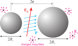
Figure 1: (color online) Top: Sketch of a granular ferroelectric (GFE) material with two metal contacts (source & drain). Bottom: Sketch of a pair of grains embedded in a FE matrix with radii $R_{1}$ and $R_{2}$ and distance $2r$ between them. The vector $\vec{P}$ is the local electric polarization of the FE matrix and the vector $\vec{E}_{i}$ is the internal electric field appearing in the system due to the presence of charged impurities. The vector $\vec{E}_{e}$ is the applied external electric field.

Besides those fundamental properties, composite materials are promising candidates for concrete microelectronics applications. Composite ferromagnets for example, can be used in magnetic field sensors, due to a high sensitivity of their resistance to a magnetic field change. Granular ferroelectrics – subject of this work – are useful in memory Yan et al. (2011); Au et al. (2013) and capacitor Huang et al. (2007); Pecharroman et al. (2001) applications because of their hysteresic behavior and their high dielectric permittivity.

The most interesting and complex aspects of these hybrid systems are their electron transport properties. In particular in (nano) granular materials, several fundamental physical phenomena have to be taken into account in order to develop a theory for the electron conductivity. In this respect the most important are Coulomb blockade Efetov and Tschersich (2003); Beloborodov et al. (2005, 2003), grain boundaries Beloborodov et al. (2007a), and quantum interference effects Biagini et al. (2005); Beloborodov et al. (2004). The transport properties of composite systems are determined by i) the material and the morphology of individual grains and ii) the nature of the coupling between grains. The conducting grains themselves can be made out of metallic Beloborodov et al. (2005), superconducting Shapira and Deutscher (1983); Hadacek et al. (2004); Skrzynski et al. (2002), or ferromagnetic Beloborodov et al. (2007b); Salvato et al. (2012) materials in various sizes and shapes. The effective coupling strength between grains can be controlled by the materials in which the grains are embedded (the matrix), the grain shape and the nearest-neighbor distance distribution. A typical matrix could be an insulator, a semiconductor, or ligants keeping the grains apart.

Most investigations that address composite (nano) materials dealing with transport physics consider the grains themselves and the emerging transport properties of large grain arrays. In contrast, here we investigate the situation, where the most interesting features of the electron transport appear and are controlled by the insulating matrix. In particular, we investigate composite materials consisting of normal metallic grains embedded in a ferroelectric (FE) matrix, Ryu et al. (2006); Wan et al. (2005); Zhong et al. (2007) see Fig. 1. In the following we refer to these systems as composite ferroelectrics or more precisely as granular ferroelectrics (GFEs).

Recently composite materials and low-dimensional structures based on ferroelectric matrices attracted a lot of attention, see, e.g. Refs. Scott (2007); Sinsheimer et al. (2012); Callori et al. (2012); Dawber et al. (2003); Wang et al. (2007); Zhang et al. (2007); Ortega et al. (2012); Dawber et al. (2005); Chanthbouala et al. (2012). However, theoretical investigations of the electron transport in GFEs was limited to the case of rather large intergrain distances, where the GFEs are practically insulators. It was shown that in the limit of weak external electric fields the conductivity of GFEs strongly depends on the correlation function of the local polarization and the microscopic internal electric field. Udalov et al. (2013)

In this paper we study electron transport in GFEs in a wide range of external parameters (electrical field and temperature) that cover not only the insulating, but also the semiconducting and the metallic regimes. In addition to the dependence of the tunneling matrix elements on the electric polarization of the ferroelectric matrix, which can be tuned by temperature and applied electric field Udalov et al. (2013), we also consider two – so-far unexplored – effects: i) the dependence of the Coulomb gap on the dielectric permittivity of the ferroelectric matrix, which in turn is controlled by temperature and external field; and ii) the hysteresis behavior of the ferroelectric matrix.

Recently, transport properties of composite ferroelectric materials were studied experimentally Au et al. (2013). It was shown that GFEs exhibit two important features: i) switching between different resistive states and ii) a current voltage hysteresis. At the end of this work, we will discuss these experimental findings based on our theoretical results.

In the out-of-equilibrium regime GFEs are particularly interesting for applications and we will discuss the possibility to use these materials as memristors (see e.g. Ref. Chanthbouala et al., 2012 and Refs. therein).

The paper is organized as follows: In section II we introduce the model of GFEs and calculate the thermodynamic properties of GFEs close to the transition point. In Section III we study transport properties of GFEs. We discuss our results in Section IV. Our summary is given in the conclusion section V. Finally, we present some estimates for typical materials and discuss the applicability of our results in Appendix A.

II Microscopic model of composite ferroelectrics

II.1 Model

Let us start with our model for composite ferroelectrics. An important feature of GFEs is the electrostatic disorder in the system. This disorder has two origins: i) a spatially dependent local anisotropy induced by the grain boundaries; and ii) a strongly inhomogeneous microscopic internal electric field, $\vec{E}_{i}$. This internal field, generated by charged impurities, see Fig. 1, is effectively screened and its magnitude between two particular grains is defined by the closest impurity located in the FE matrix Beloborodov et al. (2007a), $|\vec{E}_{i}|=E_{i}\sim e/(r^{2})\sim 10^{7}-10^{9}$ V/m with $r$ being the distance from the closest carrier trap, which is of order of a few nm. This field interacts with the ferroelectric matrix influencing the microscopic distribution of the polarization $\vec{P}$ of the ferroelectric order parameter and leading to spatial fluctuations of the dielectric permittivity of the ferroelectric matrix. In addition to the internal, $\vec{E}_{i}$, and external, $\vec{E}_{e}$, fields, the temperature, $T$, also influences the microscopic structure of the polarization and the dielectric constant.

Granularity introduces additional energy parameters into the problem Beloborodov et al. (2007a): each nanoscale cluster is characterized by (i) the charging energy $E_{C}=e^{2}/(\epsilon a)$, where $e$ is the electron charge, $\epsilon$ the dielectric constant, and $a$ the granule size, and (ii) the mean energy level spacing $\delta$. The charging energy associated with nanoscale grains can be as large as several hundred Kelvins and we require that $E_{c}/\delta\gg 1$. This condition defines the lower limit for the grain size: $a_{l}=(\epsilon/e^{2}\nu)^{1/(D-1)}$, where $\nu$ is the total density of states at the Fermi surface (DOS) and $D$ the grain dimensionality.

The internal conductance of a metallic grain is much larger than the inter-grain tunneling conductance, which is a standard condition for granularity. The tunneling conductance is one of the main parameters that controls the macroscopic transport properties of the sample Beloborodov et al. (2007a).

The most active regions in the FE matrix are those with the smallest distance between neighboring grains where electrons can tunnel, see Fig. 1. We describe these regions as quasi-two dimensional flat interfaces. In composite materials each grain has several neighbors and we enumerate different pairs of grains (not the grains themselves) by index $i$. Each pair of grains is characterized by its interface normal ${\vec{n}_{i}}=\vec{r}_{i}/|\vec{r}_{i}|$, where $\vec{r}_{i}$ is the vector connecting two grains. For grains of equal sizes there is no preferable direction (sign) of the local normal $\vec{n}_{i}$. Therefore, we assume without loss of generality that, $(\vec{n}_{i}\cdot\vec{x}_{0})>0$ where $\vec{E}_{e}=E_{e}\vec{x}_{0}$ with $\vec{x}_{0}$ being the direction of $x$-axis. This condition defines the direction of vector $\vec{n}_{i}$.

For two-dimensional interfaces the electric polarization is perpendicular to the interface, i.e., directed along the surface normal. Since the correlation length of the ferroelectric order parameter can be of the order of $1$ nm for temperatures not very close to the critical temperature we can assume that the local polarization $\vec{P}$ follows the local normal vectors $\vec{n}_{i}$, see Appendix A for details.

We also assume that external, $\vec{E}_{e}$ and internal, $\vec{E}_{i}$ electric fields do not change the orientation of the polarization (only the sign of the polarization can be changed by the electric field). We describe the internal and external electric fields by two angles $\theta_{i,i}$ and $\theta_{e,i}$ with respect to the normal $\vec{n}_{i}$.

Next we discuss important thermodynamic characteristics controlling the electron transport in GFE. First, we discuss the properties of local polarization and susceptibility concentrating on a single ferroelectric interlayer between pair of grains. Second, we consider average quantities of GFE. Finally, we discuss the hysteresis phenomena appearing in GFE.

II.2 Local polarization and susceptibility

Next, we discuss the properties of local polarization and susceptibility. To simplify our notations we will omit the grain pair index $i$ in the following.

The local polarization $\vec{P}$ can be written as $\vec{P}=P(E_{\vec{n}})\vec{n}$ with $E_{\vec{n}}=E_{e}\cos(\theta_{e})+E_{i}\cos(\theta_{i})$. To describe the polarization $P(E_{\vec{n}})$ we use the Landau-Ginzburg-Devonshire theory Devonshire (1949); Falk (1980); Strukov and Levanyuk (1998); Ong et al. (2001); Chandra and Littlewood (2007) with the free energy density written in the form

$$F=F_{0}+\alpha P^{2}+\beta P^{4}-E_{\vec{n}}P.$$ (1)

Here $F_{0}$ is the polarization independent part of the free energy density. The validity of the mean field theory in thin ferroelectrics is discussed in the Appendix A. Close to the transition temperature $T_{\operatorname{\mathrm{\scriptscriptstyle C}}}$ the parameter $\alpha$ has the form $\alpha=\eta(T-T_{\operatorname{\mathrm{\scriptscriptstyle C}}})$, and $\beta$ does not depend on temperature Strukov and Levanyuk (1998). Equation (1) does not take into account the non-uniformity of the polarization $P$. All transport characteristics for an arbitrary FE can be obtained if the function $P(E_{\vec{n}})$ is known.

Above the transition temperature $T_{\operatorname{\mathrm{\scriptscriptstyle C}}}$ a non-zero polarization $P$ appears only for a finite electric field. Below $T_{\operatorname{\mathrm{\scriptscriptstyle C}}}$ a spontaneous polarization appears even for zero electric field.

A hysteresis loop exists, as usual, only below the transition temperature $T_{\operatorname{\mathrm{\scriptscriptstyle C}}}$. Switching between two branches of hysteresis loop occurs at the switching field $E_{s}=4\alpha\sqrt{|\alpha|/6\beta}/3$.

The local dielectric susceptibility along the direction $\vec{n}$ is given by: Strukov and Levanyuk (1998) $\chi_{\vec{n}}=\partial_{E_{\vec{n}}}P=(2\alpha+12\beta P^{2}(E_{\vec{n}}))^{-1}$. For temperatures below the transition temperature, $T<T_{\operatorname{\mathrm{\scriptscriptstyle C}}}$, the dielectric susceptibility $\chi_{\vec{n}}$ diverges at the points of the polarization switching $E_{\vec{n}}=\pm E_{s}$. For temperatures above $T_{\operatorname{\mathrm{\scriptscriptstyle C}}}$ the permittivity $\chi_{\vec{n}}$ is a smooth function without any singularities. The above discussions are valid for local properties of composite materials only.

II.3 Macroscopic susceptibility and correlation function

The electron transport in GFE is controlled by the average electrical susceptibility $\overline{\chi}$ and the correlation function of local electric field and local polarization of FE matrix $C=\left\langle(\vec{E}_{i}+\vec{E}_{e})\cdot\vec{P}\right\rangle$. Using the microscopic model of FE matrix discussed in Sec. II.1 we calculate $\overline{\chi}$ and $C$ by averaging over the mutual orientation of local normal $\vec{n}$, internal $\vec{E}_{i}$, and external $\vec{E}_{e}$ electric fields. The details of these calculations are relocated into Appendix B.

The final result for temperature dependence of dielectric susceptibility in Eqs. (18) and Eq. (19) is shown in Fig. 2. The susceptibility has its maximum value $\overline{\chi}_{\|}=\overline{\chi}_{\perp}=4^{2/3}/(24\beta^{1/3}E_{i}^{2/3})$ for temperature $T=T_{\operatorname{\mathrm{\scriptscriptstyle C}}}$ and zero external field, $E_{e}=0$, and it increases with decreasing internal field. The derivative of susceptibility has a jump at the transition point following from the divergence of the microscopic susceptibility $\chi_{\vec{n}}$ appearing at the Curie temperature $T_{\operatorname{\mathrm{\scriptscriptstyle C}}}$. However, in real ferroelectrics this behavior is absent due to order parameter fluctuations. Therefore the kink in the average susceptibility $\overline{\chi}$ is smeared. There is also another peculiarity in the temperature dependence of the susceptibility $\overline{\chi}$. at finite external electric field $E_{e}$ due to the hysteresis behavior of the polarization of FE matrix. This peculiarity is located at the switching temperature $T_{S}$, defined by the equation $E_{s}(T_{S})=<|E_{\vec{n}}|>$, with $E_{s}$ being the switching field and brackets standing for averaging over all pairs of grains.

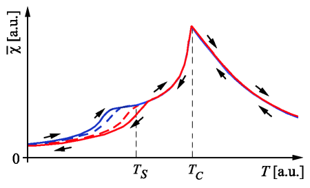
Figure 2: (color online) Average dielectric susceptibility $\overline{\chi}$ vs. temperature. The solid lines correspond to the longitudinal $\overline{\chi}_{\parallel}$, Eq. (18), and the dash lines correspond to the perpendicular $\overline{\chi}_{\perp}$, Eq. (19), components of susceptibility $\overline{\chi}$. The behavior is shown for both hysteresis branches. Arrows indicate the path around the hysteresis loop for fixed external electric field $E_{e}=E_{i}/3$. $T_{C}$ and $T_{S}$ are the Curie and the switching temperatures, respectively. The derivative of susceptibility has a jump at the transition point following from the divergence of the microscopic susceptibility $\chi_{\vec{n}}$ appearing at the points of polarization switching ($E_{s}$ or $T_{S}$). However, in real ferroelectrics this behavior is absent due to order parameter fluctuations. Therefore the kink in the average susceptibility $\overline{\chi}$ is smeared.

The behavior of the correlation function $C$ is shown in the inset in Fig. 8. It has two branches below the critical temperature $T_{C}$ due to hysteresis behavior of local polarization. The upper branch corresponds to the case of local polarization directed along the applied electric field, in this case the correlation function is positive, $C>0$. The lower branch corresponds to the situation with local polarization directed oppositely to the electrical field, in this case $C<0$. Above the Curie temperature $T_{C}$ the correlation function $C$ has only one branch and monotonically decreases with increasing the temperature $T$.

II.4 Hysteresis

The properties of GFE depends on it’s history. To study the hysteresis phenomena, we first apply a large positive external electric field ($E_{e}>0$) and then decrease its magnitude until reaching a large negative field ($E_{e}<0$) [upper branch], which is finally reversed until the initial electric field value is reached [lower branch], thus closing the hysteresis loop. As a result the temperature dependence has two branches.

III Electron transport in composite ferroelectrics

In this section we discuss the transport properties of composite ferroelectrics. The ferroelectric matrix influences the transport properties in two ways:

i) Through the dependence of the local tunneling conductance between two grains $\tilde{g}_{t}$ on the polarization, $\tilde{g}_{t}=g^{0}_{t}(1+\zeta((\vec{E}_{i}+\vec{E}_{e})\cdot\vec{P})+\mu((\vec{E}_{i}+\vec{E}_{e})\cdot\vec{r})(\vec{P}\cdot\vec{r}))$ with $g_{t}^{0}$ being the tunneling conductance in the paraelectric state and $\zeta$, $\mu$ being phenomenological constants, and $\vec{r}$ being the vector connecting the grains (see Fig. 1).

ii) Through the dependence of Coulomb gap

$$E_{C}=e^{2}/(\epsilon a).$$ (2)

The Coulomb blockade leads to the appearance of the Mott gap, $E_{C}$, allowing for an additional control of the transport properties by external electric field and temperature. This effect is especially pronounced for weak external electric fields and low temperatures, where transport is due to electron cotunneling Beloborodov et al. (2007a). For strong external fields the Coulomb blockade is suppressed, thus leading to a weak dependence of the conductivity on the dielectric permittivity.

There are several transport regimes in composite materials depending on the coupling between the grains. For weak coupling, low temperatures, and small electric fields the electron transport is due to electron cotunneling. This mechanism involves electron energy levels inside the Mott gap. At higher temperatures electrons can be excited directly above the Coulomb gap. Thus, the activation transport mechanism becomes important. At even higher temperatures, $T\geq E_{C}$, the electron transport becomes metallic.

We mention that for temperatures approaching the transition temperature $T_{\operatorname{\mathrm{\scriptscriptstyle C}}}$ the dielectric permittivity $\epsilon$ increases leading to a decrease of the charging energy $E_{C}=e^{2}/\epsilon a$, with $\epsilon$ being the permittivity of the whole sample including the ferroelectric matrix and metallic grains. Assuming that the metal dielectric constant is very large (infinite) at zero frequency we can write for sample permittivity

$$\epsilon=\epsilon_{fe}(\Omega/\Omega_{fe}),\hskip 14.22636pt\epsilon_{fe}=1+4\pi\overline{\chi},$$ (3)

were $\Omega$ and $\Omega_{fe}$ are the sample and ferroelectric matrix volume, respectively.

The value of the dielectric permittivity, $\epsilon_{A}$, where activation transport becomes important is $\epsilon_{A}=e^{2}\xi/(a^{2}k_{B}T)$, where $\xi$ is the electron localization length defined below Beloborodov et al. (2007a). If the maximum of $\epsilon=1+4\pi\overline{\chi}$ is large at temperatures approaching $T_{\operatorname{\mathrm{\scriptscriptstyle C}}}$, $\epsilon>\epsilon_{A}$ then one observes activation transport in a temperature region $T^{<}_{A}<T<T^{>}_{A}$, where temperatures $T^{<}_{A}$ and $T^{>}_{A}$ are defined by the condition $\epsilon(T^{<,>}_{A})=\epsilon_{A}(T^{<,>}_{A})$. For grain sizes $a=4$nm and temperature $T\approx 400$ K one finds $\epsilon_{A}\approx 9$.

Metallic regime appears for temperatures $T_{M}\geq e^{2}/(\epsilon(T_{M})a)$.

Usually ferroelectrics have a very large dielectric constants in the vicinity of the transition temperature leading to the merallic transport in this temperature region.

Another important parameter controlling the GFE conductivity is the external electric field, $E_{e}$. The phonon mediated electron cotunneling occurs for weak external electric fields, $E_{e}<E^{*}=T/(e\xi)\approx 10^{6}-10^{8}$ V/m. For electric fields $E_{e}>E^{*}$ the electron cotunneling is mediated by external electric field and does not depend on temperature.

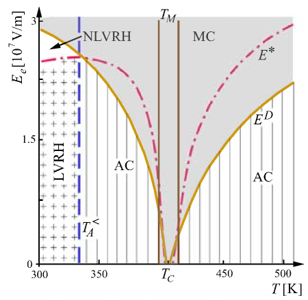
Figure 3: (color online) Transport phase diagram of granular ferroelectrics in coordinates of the external electric field $E_{e}$ vs. temperature $T$. $T_{C}$ is the Curie temperature. AC (shaded region) denotes the activation conductivity, LVRH (cross filled region) and NLVRH (unfilled region) stand for linear and non-linear electron cotunneling, respectively. MC (colored region) stands for metallic conductivity. The blue line $T_{A}^{<}$ describes the transition to activation transport; the brown lines $T_{M}$ describe the transition from activation to metallic regimes, these lines have a physical meaning outside the metallic regime only (colored region - MC) The electric field $E^{D}$ describes the transition to the metallic regime. The field $E^{*}$ shows the boundary between the linear and non-linear hopping regimes. This field has physical meaning outside the metallic regimes only, since inside the metallic region the VRH contribution to the conductivity is negligible.

In addition, there is another characteristic field $E^{D}=e/(a^{2}\epsilon)\approx 10^{6}-10^{8}/$ V/m. For external fields larger than $E^{D}$ the electron transport is metallic. The ratio of the two fields is $E^{D}/E^{*}=(E_{C}/T)\cdot(\xi/a)$.

We summarize the different transport regimes of granular ferroelectrics as a function of external electric field and temperature in the reversible case in Fig. 3 for the following set of parameters: $T_{\operatorname{\mathrm{\scriptscriptstyle C}}}=400$ K, $\eta=0.01$ 1/K, $\beta=3\cdot 10^{-2}$, this corresponds to BaTiO₃; parameter $\zeta=10^{-10}$ is chosen to be small such that hysteresis effects can be neglected; $g^{t}_{0}=0.2$, $a=5$ nm, $\Omega/\Omega_{fe}=1.5$, the last parameter corresponds to a $1$ nm distance between the grains, and $E_{i}=7\cdot 10^{8}$ V/m. Below we discuss three transport regimes in more details.

III.1 Electron cotunneling

At low external electric fields and weak coupling between the grains the electron transport is due to the cotunneling mechanism. The most important parameters are the average tunnel conductance $g_{t}(P)$ and the electron localization length $\xi$ Beloborodov et al. (2007a). The former is given by

$$g_{t}(P) = g^{0}_{t}\left(1+\operatorname{\mathcal{C}}_{\rm eff}\right)\,\,\,\text{with}$$ (4)

$$\operatorname{\mathcal{C}}_{\rm eff} \equiv \left\langle\vec{E}\cdot\vec{P}_{\rm eff}\right\rangle$$ (5)

being the correlation function of the effective polarization with $\vec{P}_{\rm eff}=\zeta\vec{P}+\mu\vec{r}_{12}(\vec{P}\cdot\vec{r}_{12})$ and the electric field $\vec{E}=\vec{E}_{i}+\vec{E}_{e}$; vector $\vec{r}_{12}$ connects two grains; $g^{0}_{t}$ is the tunneling conductance in the paraelectric phase. The inelastic localization length $\xi$ is given by the expression Beloborodov et al. (2007a)

$$\xi=a/\ln(E^{2}_{c}/T^{2}g^{0}_{t}).$$ (6)

The conductivity in this regime is

$$\sigma_{L}=g^{0}_{t}(1+\operatorname{\mathcal{C}}_{\rm eff})\exp(-\sqrt{T^{P}_{0}/T}),$$ (7)

where $T^{P}_{0}$ is the characteristic temperature scale

$$T^{P}_{0}=T_{0}\left[1-\frac{\xi}{2a}\ln\left(1+\operatorname{\mathcal{C}}_{\rm eff}\right)\right],$$ (8)

with $T_{0}=e^{2}/(\epsilon\xi)$, Efros and Shklovskii (1975). To calculate $\operatorname{\mathcal{C}}_{\rm eff}$ one has to evaluate first the average $\left\langle(\vec{E}\cdot\vec{r}_{12})(\vec{r}_{12}\cdot\vec{P})\right\rangle$. Using Wick’s theorem one can show that $\operatorname{\mathcal{C}}_{\rm eff}=\tilde{\zeta}C$, where $\tilde{\zeta}=\zeta+\mu\left\langle\vec{r}^{2}_{12}\right\rangle$.

In the non-linear (field driven) cotunneling regime with external electric fields $E_{e}>E^{*}$, the conductivity has the following form:

$$\sigma_{NL}=g^{0}_{t}(1+\operatorname{\mathcal{C}}_{\rm eff})\exp(-(E^{W}_{0}/E_{e})^{1/2}).$$ (9)

Here $E^{W}_{0}=T^{P}_{0}/e\xi$ is the characteristic electric field with temperature $T^{P}_{0}$, Shklovskii (1973).

III.2 Metallic transport

For strong external electric field, $E_{e}>E^{D}$, the Coulomb blockade is suppressed leading to metallic transport. The main contribution to conductivity in this regime is given by the expression Beloborodov et al. (2007a)

$$\sigma_{D}=2e^{2}g_{t}/a=2e^{2}g^{0}_{t}(1+\operatorname{\mathcal{C}}_{\rm eff})/a.$$ (10)

III.3 Activation transport

Another regime which is shown in Fig. 3 is the region with activation transport where the main contribution to the conductivity is due to electron driven by the temperature to the conduction band, above the Mott gap

$$\sigma_{A}\sim\exp(-[E_{C}/T]).$$ (11)

IV Discussion

IV.1 Metal-insulator transition

In this section we discuss two transport phenomena specific to granular ferroelectrics starting our discussions with the metal-insulator transition.

The transport phase diagram in Fig. 3 shows two transitions for temperatures close to the critical temperature $T_{C}$ and weak applied electric fields: i) from VRH to activation transport and ii) from activation to a metallic transport. These transitions are possible due to a strong dependence of the Coulomb gap on temperature.

The dependence of the dielectric permittivity and the Coulomb gap on temperature is shown in Fig. 4. The curves are plotted for the same set of parameters as used in the previous section for the calculation of the transport phase diagram and for external electric field we use $E_{e}=6\cdot 10^{6}$ V/m. The dielectric permittivity of ferroelectric materials diverges close to the transition temperature on both sides of the transition as $\epsilon\sim 1/|(T-T_{C})|$. However, due to the granular morphology and the internal electric field the permittivity peak is smeared.

The transition from VRH to activation conductivity can be understood as follows: Away from the transition temperature $T_{C}$ the dielectric permittivity $\epsilon$ of the FE matrix is small and the Coulomb gap is large. Therefore there are no electrons in the conduction band at zero temperature, thus the GFE is an insulator. The only transport mechanism here is VRH. The increase of temperature leads to the reduction of the Coulomb gap and to the increase of the number of electrons in the conduction band (above the Mott gap). The activation conductivity becomes more important than VRH at temperatures $T\geq T_{M}$.

The transition from activation to the metallic regime can occur in two ways (see Fig. 3): i) the temperature driven, for external fields less than $E_{e}<5\cdot 10^{6}$V/m. In this case the Mott gap disappears for temperatures approaching the Curie point leading the GFE to the metallic state. This transition occurs at temperatures $T=T_{M}$.

ii) the field driven, for external fields larger than $E_{e}>5\cdot 10^{6}$V/m. In this case the voltage between the nearest neighbor grains becomes comparable with the Mott gap pushing electrons to the conduction band. This transition occurs at external electric field $E_{e}=E^{D}$.

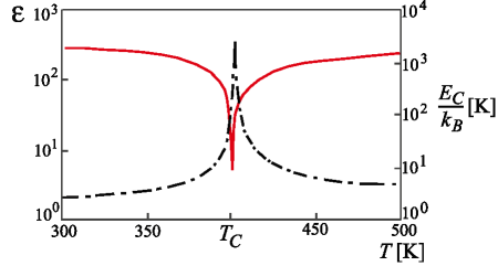
Figure 4: (Color online) Dielectric permittivity $\epsilon$ (solid line), Eq. (3), and Coulomb gap $E_{C}$ (dash line) of granular ferroelectrics, Eq. (2), vs. temperature at fixed external electric field, $E_{e}=6\cdot 10^{6}$ V/m. $T_{C}$ is the Curie temperature.

Figure 5 shows the metal-insulator transition corresponding to the temperature dependence of the Coulomb gap presented in Fig. 4. Figure 5 is plotted for small susceptibility $\chi$, where hysteresis effects can be neglected. For these parameters there are two clear transitions: i) from VRH to activation transport at temperatures $T=T_{A}^{<}$ and ii) from activation to metallic transport at external electric field $E_{e}=E^{D}$. The field driven transition occurs when the horizontal line in the transport phase diagram in Fig. 3 corresponding to the external field $E_{e}=6\cdot 10^{6}$ V/m crosses the $E^{D}$ curve.

It follows from Fig. 5 that the conductivity of GFE increases three orders of magnitude in a rather narrow temperature range. This is an unexpected result because usually conductivity decreases in the vicinity of a phase transition due to scattering of electrons on fluctuations of the order parameter. Here we have the opposite situation with decreasing resistivity. This behavior can be utilized to built a GFE thermometer for precise temperature measurements using an appropriate gauge. It is worth to mention that this non-trivial behavior is a peculiarity of granular ferroelectrics and cannot be observed in the tunnel junctions with ferroelectric barrier.

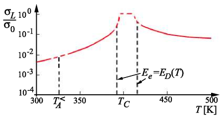
Figure 5: (Color online) Conductivity $\sigma$ of GFE, with $\sigma_{0}=2e^{2}g^{0}_{t}/a$ being the metallic conductivity in the paraelectric phase, vs. temperature at fixed external electric field $E_{e}=6\cdot 10^{6}$ V/m. Variable range hopping and electron cotunneling, Eq. (7), is the main transport mechanism for temperatures $T<T_{A}^{<}$. Close to the transition temperature $T_{C}=400$ K the transport is metallic, Eq. (10). Between these two regions the conductivity has activation behavior, Eq. (11).

IV.2 Memory effects

In the previous section we discussed the influence of the FE matrix on the Coulomb gap of the GFE system. Here, on the other hand, we study explicitly the influence of the hysteretic behavior on the electron transport in GFEs. Due to the hysteresis in a ferroelectric matrix, the resistivity of GFEs has two states depending on the history for any external electric field. Figure 6 shows the behavior of the GFE conductivity on the external electric field with two distinctive features:

i) The first feature is the metal-insulator transition appearing for increasing electric field. For weak external field the GFE is an insulator since all electronic states are localized due to Coulomb blockade. At strong external electric field electrons can overcome the Coulomb gap moving the GFE into a metallic state. The transition between these two states occurs for the electric field $E=E^{D}$. Figure 6 shows the transition between activation and metallic regimes for temperature $T=350K$.

ii)The second feature is the hysteresis behavior. The most striking manifestation of the hysteresis is the strong dependence of the transition field $E^{D}$ on the state of a ferroelectric matrix.

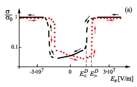
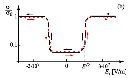
Figure 6: (color online) Conductivity $\sigma$, with $\sigma_{0}=2e^{2}g^{0}_{t}/a$ being the metallic conductivity in the paraelectric phase, vs. external electric field $E_{e}$ at fixed temperature $T=350$ K ($E^{D}\approx 1.5\cdot 10^{7}$ V/m). The solid and dotted lines correspond to the two hysteresis branches. The arrows show the direction, the hysteresis loop is followed. There are two different situations: (a) The average internal field $E_{i}=5.7\cdot 10^{7}$ V/m is less than the FE switching field $E_{s}=6.3\cdot 10^{7}$ V/m and (b) The average internal field $E_{i}=5.7\cdot 10^{7}$ V/m is larger than the switching field $E_{s}=3.9\cdot 10^{7}$ V/m. For internal fields $E_{i}>E_{s}$, there is no difference between fields $E^{D}_{<}$ and $E^{D}_{>}$.

We introduce the fields corresponding to different hysteresis branches as $E^{D}_{>,<}$. The difference between these fields is controlled by the internal parameters of the system. One can distinguish two different situations. The curves shown in Fig. 6(a) correspond to the situation when the average internal field $E_{i}=5.7\cdot 10^{7}$ V/m is smaller than the FE switching field $E_{s}=6.3\cdot 10^{7}$ V/m. In this limit the effect is pronounced. In the opposite limit, $E_{i}>E_{s}$, there is no difference between $E^{D}_{<}$ and $E^{D}_{>}$, see Fig. 6(b)). Figures 6(a) and 6(b)) are plotted for the following set of parameters: the tunneling conductance $g^{t}_{0}=0.2$, the grain size $a=5$ nm, $\Omega/\Omega_{fe}=1.5$, parameters $\alpha$ and $\beta$ are chosen to get the above mentioned switching fields, and $\zeta=10^{-7}$.

The transition field $E^{D}=e^{2}/(a^{2}\epsilon)$ is determined by the average dielectric permittivity, $\epsilon$. Thus to understand the two limits mentioned above one has to study the dependence of the GFE dielectric permittivity $\epsilon$ on the external electric field, $E_{e}$. Figure 7 shows the dependence of the local FE permittivity $\epsilon$ on the local electric field consisting of internal field $\vec{E}_{i}$ and external field $\vec{E}_{e}$. The two curves correspond to the two hysteresis branches. The permittivity of the whole GFE can be found by averaging over all orientations of the internal field, see Sec. II. The local susceptibility should be averaged over the field interval [$E_{e}-E_{i},E_{e}+E_{i}$]. If the internal field $E_{i}\gg E_{s}$, see Fig. 7(a), then the averaging produces the same result for both branches and one gets the same dielectric permittivity unless the external electric field is less than $E_{i}-E_{s}$. Therefore if the transition field $E^{D}<E_{i}-E_{s}$ there is no difference between $E^{D}_{<}$ and $E^{D}_{>}$, see Fig. 6(b). If $E_{i}<E_{s}$, see Fig. 7(b), then the averaged dielectric permittivity is different for the two branches at any finite external field. Therefore in this case $E^{D}_{<}\neq E^{D}_{>}$.

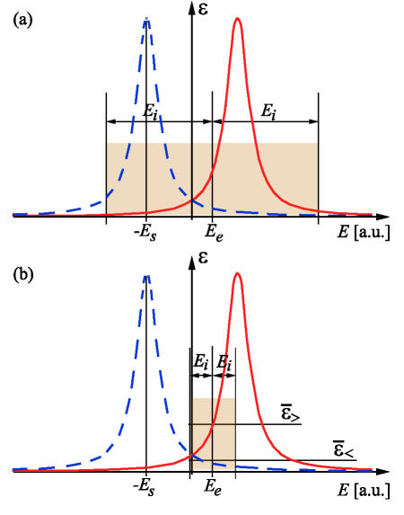
Figure 7: (color online) The local permittivity $\epsilon$ of the FE matrix vs. local electric field, $E=E_{e}+E_{i}$, with $E_{e}$ and $E_{i}$ being the external and internal electric fields, respectively. Solid and dash lines correspond to two hysteresis branches. According to the procedure described in the Sec. II the dielectric permittivity of the whole GFE is the average of the local permittivity over different internal field orientations. The filled area shows the region of averaging. There are two different situations: (a) The internal field $E_{i}$ is larger than the switching field $E_{s}$ and (b) The internal field $E_{i}$ is less than the switching field $E_{s}$.

IV.3 Comparison with experiment

Here we compare our results with available experimental data on electron transport in composite ferroelectrics Au et al. (2013). Experimentally, the current voltage characteristics has two peculiarities [see Fig. 3(a) of Ref. Au et al. (2013)]: i) switching of the resistivity at a certain voltage and ii) a current voltage hysteresis effect. As can be seen in Fig. 6, the same features are present in our model: i) The current jump appears due to a transition from the insulating phase with cotunneling transport mechanism to a metallic phase with suppressed Coulomb blockade. ii) The memory effect appears due to a ferroelectric matrix hysteresis. Thus, the data of Ref. Au et al. (2013) can be qualitatively described by our theory.

We note, that our Fig. 6 shows bipolar switching behavior in contrast to the unipolar switching mechanism reported in Ref. Au et al. (2013). This difference is related to the fact that we assume an infinite relaxation time of the polarization of the FE matrix here. However, if the relaxation time is comparable to the time the loop is traversed, unipolar switching is possible as well.

We note, that the variation of the switching voltage for different hysteresis loops observed in Ref. Au et al. (2013) is an effect, which cannot be described by the framework presented here. The switching of the resistance appears when the Coulomb blockade is suppressed by an external field along a single conductive chain. The first conductive chain is determined by the current distribution of the electrons in the metal particles and impurities. Therefore it can be different for different sweeping loops and so does the switching voltage. In our consideration we average the current over a large system size smearing out the charge distribution fluctuations. Therefore the switching voltage is time independent. This is not the case in Ref. Au et al. (2013), since the thickness of the GFE in their experiment is rather small.

We also mention that current-voltage hysteresis loops were observed in granular metals Lee et al. (2010), i.e., in systems consisting of metallic grains embedded into a simple insulator. In this case memory effects can be understood using the Simmons-Verderber model Simmons and Verderber (1967), where electrons are trapped by defects inside the insulator (the metal particles in the case of granular metals) and stored in these defects for long times. This modifies the potential profile for electrons moving through the system and changes the resistance. This model can be also used for a description of current voltage hysteresis in GFEs. In order to discriminate between these two effect on can heat the system above the ferroelectic Curie temperature, such that the contribution of the hysteresis due to the FE matrix can be neglected.

IV.4 Influence of the FE matrix on the electron transport in the metallic regime

In the metallic regime the dielectric permittivity of the FE matrix does not play an important role on the electron transport of GFEs. However, it influences the tunneling conductance between grains. In this region the correlation function $C$ of local electric polarization and the local electric field becomes important. Figure 8 shows the behavior of the conductivity in the metallic region (external field $E_{e}=3\cdot 10^{7}$ V/m) vs. temperature. The parameters of the GFE are chosen to be the same as for the transport phase diagram except for parameter $\zeta$, which is now larger $10^{-7}$. The presence of the FE matrix leads to the occurrence of two resistive states. The upper branch corresponds to the case of local polarization $P$ of FE matrix co-directed with the external electric field $E_{e}$. In this case the correlation function is positive, $C>0$ and the intergrain tunneling conductance and thus the conductivity increase. The lower branch corresponds to the case of local polarization $P$ counter-directed to the external field (due to the hysteresis phenomenon) leading to the negative correlation function $C<0$. In this case the intergrain tunneling conductance decreases resulting in the decrease of conductivity $\sigma_{D}$. For temperatures $T>T_{\operatorname{\mathrm{\scriptscriptstyle C}}}=400$ K the memory effects are absent leading to a single resistive state.

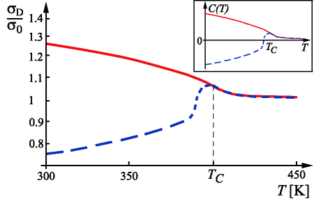
Figure 8: (color online) Conductivity of a GFE vs. temperature in the metallic regime, Eq. (10), at fixed external electric field $E_{e}=3\cdot 10^{7}$ V/m. Solid and dash lines correspond to the two hysteresis branches. The inset shows the behavior of the correlation function $C(T)$ on temperature, Eq. (21). The conductivity in the metallic regime is controlled by the correlation function.

V Conclusion

We investigated the electron transport in composite ferroelectrics consisting of metallic grains embedded in a ferroelectric matrix and show that depending on the external electric field and temperature three transport regimes are possible: 1) multiple electron cotunneling, 2) sequential tunneling, and 3) metallic transport. We showed that the crossover between different regimes can be studied by changing the temperature or the external electric field leading to a strongly non-linear conductivity behavior and large conductivity jumps. The microscopic reason for the crossover between different regimes is the changing of the Coulomb gap due to the variation of dielectric permittivity of the ferroelectric matrix under the influence of temperature or electric field. This interesting effect arises due to the interference of granular morphology and ferroelectric matrix.

Another peculiarity of electron transport in composite ferroelectrics occurs due to the hysteretic behavior of the ferroelectric matrix. It leads to the existence of two different intermediate states with different average electrical polarization and correlation function of microscopic electric field and microscopic polarization. These two states have different conductivity.

We showed that our theory is in qualitative agreement with recent experiments on transport properties of granular ferroelectrics.

In addition, we show that the main parameters determining the transport in composite ferroelectrics are: 1) the correlation function of intrinsic microscopic field and the local electric polarization and 2) the dielectric permittivity of the ferroelectric matrix.

VI Acknowledgments

A. G. was supported by the U.S. Department of Energy Office of Science under the Contract No. DE-AC02-06CH11357. I. B. was supported by NSF under Cooperative Agreement Award EEC-1160504.

Appendix A Applicability of the model

In this appendix we consider the applicability of our method. It is based on a mean field approach, meaning that fluctuations around the order parameter are small and therefore cannot suppress the order parameter.

First, we estimate the correlation length of electrical order parameter, $r_{c}$, which is given by the expression, $r_{c}=\sqrt{g/(\alpha(T-T_{\operatorname{\mathrm{\scriptscriptstyle C}}}))}$, with $\alpha$ and $g$ being the constants in the expression of the free energy density of the ferroelectric, $F=F_{0}+\alpha(T-T_{\operatorname{\mathrm{\scriptscriptstyle C}}})P^{2}+\beta P^{4}+g(\delta_{\vec{r}}P)^{2}$. The parameters $g$ and $\alpha$ can be estimated as $\alpha=0.01$ K^-1, $g\approx 3\cdot 10^{-22}$ cm², Fridkin et al. (0010). In our consideration the direction of the polarization $P$ is determined by the local anisotropy field appearing due to grain boundaries. This assumption is valid if the ferroelectric domain wall thickness (or correlation length) is less than the characteristic length scale of the spatial variations of the anisotropy field. The latter is of the order of the grain size ($\sim 5$ nm). Therefore for correlation length $r_{c}<5$ nm our consideration is justified. With the parameters provided above this inequality holds for temperatures $|T-T_{\operatorname{\mathrm{\scriptscriptstyle C}}}|>12K$.

Second, the mean field theory for $3d$ samples is valid for temperatures Landau and Lifshitz (1980)

$$\frac{k_{B}T_{\operatorname{\mathrm{\scriptscriptstyle C}}}\,\overline{\chi}}{r_{c}^{3}}\ll\frac{\alpha(T-T_{\operatorname{\mathrm{\scriptscriptstyle C}}})}{\beta}=2P_{0}^{2},$$ (12)

where $k_{B}$ is the Boltzman constant, $\overline{\chi}$ is the macroscopic susceptibility, $\beta$ is the constant in the expression for the free energy density of the ferroelectric material. To estimate the l. h. s. of Eq. (12) we use the following set of parameters, Fridkin et al. (0010): $\alpha(T-T_{\operatorname{\mathrm{\scriptscriptstyle C}}})\approx 1$ ($T_{\operatorname{\mathrm{\scriptscriptstyle C}}}=400$, $T=300$, $\alpha=0.01$ K${}^{-}1$), $g\approx 3\cdot 10^{-22}$ cm². For the correlation length we find $r_{c}\approx 1.5$ nm. For these parameters Eq. (12) is satisfied.

The electrical polarization for thin ($\sim 5$nm) films of BaTiO₃ is about 0.4 C/m² (1.2$\cdot 10^{5}$ statC/cm² in cgs), Fridkin (2006). The critical thickness for this material is of order of $1$nm. For the polarization $P_{0}\approx 3\cdot 10^{5}$ statC/cm² and susceptibility $\chi\sim 1/\alpha(T-T_{\operatorname{\mathrm{\scriptscriptstyle C}}})\approx 1$ we find

$$\frac{k_{B}T_{\operatorname{\mathrm{\scriptscriptstyle C}}}\overline{\chi}}{r_{c}^{3}}\approx 10^{7}\textrm{statC}^{2}/\textrm{cm}^{4},$$ (13)

and

$$P_{0}^{2}\approx 10^{11}\textrm{statC}^{2}/\textrm{cm}^{4}.$$ (14)

Therefore inequality (12) is well satisfied at room temperature.

Decreasing the temperature one can effectively reduce the dimensionality of the sample. For the correlation length larger than the ferroelectric thickness, the three dimensional condition, Eq. (12), needs to be replaced by the following condition for the applicability of the mean field theory

$$\frac{k_{B}T_{\operatorname{\mathrm{\scriptscriptstyle C}}}\overline{\chi}}{r_{c}^{2}L}\ll\frac{\alpha(T-T_{\operatorname{\mathrm{\scriptscriptstyle C}}})}{\beta}=2P_{0}^{2},$$ (15)

where $L$ is the ferroelectric thickness. As one can see Eq. (15) is also satisfied for our set of parameters. Thus the requirement of a small correlation length in comparison with the grain sizes is the strongest restriction determining the validity of our considerations.

Appendix B Average characteristics of GFE

Here we discuss the average thermodynamic characteristics of GFE. The mutual orientation of local normal $\vec{n}$, internal $\vec{E}_{i}$, and external $\vec{E}_{e}$ electric fields is random. We introduce angles ($\theta_{e}$, $\phi_{e}$) and ($\theta_{i}$, $\phi_{i}$) describing the orientation of fields $\vec{E}_{e}$ and $\vec{E}_{i}$ with respect to the local normal, $\vec{n}$. For uniform distribution of angles ($\theta_{i}$, $\phi_{i}$) the distribution function is $\omega_{i}(\theta_{i},\phi_{i})=1/(4\pi)$. The distribution function of the angles ($\theta_{e}$, $\phi_{e}$) is described by the following expression

$$\omega_{e}(\theta_{e},\phi_{e})=\frac{1}{4\pi}\left\{\begin{array}[]{l}1+\operatorname{sign}(E_{e}),~{}0<\theta_{e}\leq\pi/2,\\ 1-\operatorname{sign}(E_{e}),~{}\pi/2<\theta_{e}\leq\pi.\end{array}\right.$$ (16)

In general, the distributions can be anisotropic for grains forming a regular array. However, here we concentrate on the isotropic case.

We now calculate the average polarization $\overline{\vec{P}}$ for finite external electric field, $\vec{E}_{e}$. For the isotropic model the average polarization is parallel to the external field $\overline{\vec{P}}=\overline{P}\,\vec{x}_{0}$. The local polarization is directed along the local normal and its projection on the positive direction is $(\vec{P}\cdot\vec{x}_{0})=P(E_{\vec{n}})|\cos(\theta_{e})|$. Also we assume that the magnitude of the internal field $|\vec{E}_{i}|$ is spatially homogeneous. The generalization for an inhomogeneous distribution of internal fields is straightforward. For the average polarization we obtain

$$\begin{array}[]{l}\overline{P}=\iint\limits^{~{}~{}2\pi}_{0}d\phi_{i}d\phi_{e}\iint\limits^{~{}~{}\pi}_{0}\sin(\theta_{i})d\theta_{i}\sin(\theta_{e})d\theta_{e}\times\\ ~{}~{}~{}~{}~{}\times P(E_{\vec{n}})|\cos(\theta_{e})|\omega_{e}(\theta_{e},\phi_{e})\omega_{i}\,.\end{array},$$ (17)

where $\omega_{e}(\theta_{e},\phi_{e})$ is the distribution function defined by Eq. 16. Note, that the average polarization does not enter directly into the expressions for the electron transport.

Besides the average polarization, an important characteristic is the average dielectric susceptibility $\overline{\chi}$. The composite material is isotropic in the paraelectric phase for zero external field an hence, the dielectric susceptibility $\overline{\chi}$ is also isotropic. However, for finite electric field it is necessary to distinguish the longitudinal and transverse dielectric permittivity. The anisotropy of $\overline{\chi}$ becomes important for an external field of the order of the internal field. For these fields the transport is metallic meaning that the Mott gap is vanishingly small. Thus the susceptibility is not important for strong fields. Below we consider the limit of strong internal fields, $E_{e}\ll E_{i}$, and introduce the coordinate system related to the field $\vec{x}_{0}$. The direction along vector $\vec{x}_{0}$ is denoted by the subscript $\parallel$ and the direction perpendicular to $\vec{x}_{0}$ is denoted by subscript $\perp$. The average longitudinal susceptibility $\overline{\chi}_{\parallel}=\partial{\overline{P}_{\parallel}}/\partial{E}_{e\parallel}$ can be calculated as follows

$$\begin{array}[]{l}\overline{\chi}_{\parallel}=\iint\limits^{~{}~{}2\pi}_{0}d\phi_{i}d\phi_{e}\iint\limits^{~{}~{}\pi}_{0}\sin(\theta_{i})d\theta_{i}\sin(\theta_{e})d\theta_{e}\times\\ ~{}~{}~{}~{}~{}\times\chi_{\vec{n}}(E_{\parallel})|\cos^{3}(\theta_{e})|\omega_{e}(\theta_{e},\phi_{e})\omega_{i}.\end{array}$$ (18)

The average transverse susceptibility $\overline{\chi}_{\perp}=\partial{\overline{P}_{\perp}}/\partial{E}_{e\perp}$ is determined by the expression

$$\begin{array}[]{l}\overline{\chi}_{\perp}=\iint\limits^{~{}~{}2\pi}_{0}d\phi_{i}d\phi_{e}\iint\limits^{~{}~{}\pi}_{0}\sin(\theta_{i})d\theta_{i}\sin(\theta_{e})d\theta_{e}\times\\ ~{}~{}~{}~{}~{}\times\chi_{\vec{n}}(E_{\parallel})|\cos(\theta_{e})|\sin^{2}(\theta_{e})\sin^{2}(\phi_{e})\omega_{e}\omega_{i}.\end{array}$$ (19)

For small external fields Eqs. (18) and (19) for the susceptibility can be simplified to

$$\begin{array}[]{l}\overline{\chi}_{\parallel}=\frac{1}{12E_{i}}\int\limits^{E_{i}}_{-E_{i}}\chi_{\vec{n}}(\varepsilon)d\varepsilon+\frac{E_{e}}{16E_{i}}(\chi_{\vec{n}}(E_{i})-\chi_{\vec{n}}(-E_{i})),\\ \overline{\chi}_{\perp}=\frac{1}{12E_{i}}\int\limits^{E_{i}}_{-E_{i}}\chi_{\vec{n}}(\varepsilon)d\varepsilon+\frac{E_{e}}{32E_{i}}(\chi_{\vec{n}}(E_{i})-\chi_{\vec{n}}(-E_{i})).\end{array}$$ (20)

Above the Curie temperature, $T>T_{\operatorname{\mathrm{\scriptscriptstyle C}}}$ the second terms of both equations are zero and therefore the susceptibility is isotropic. It is isotropic for zero external field $E_{e}$. The lowest order expansion of $\overline{\chi}$ in external field, $E_{e}$, given in Eqs. (20), has a finite linear contribution (2nd terms). This indicates a finite remanent electric polarization at zero external field and therefore is a signature of the hysteretic behavior.

One more important characteristic quantity of composite ferroelectrics is the correlation function of electric fields and polarization $C=\left\langle(\vec{E}_{i}+\vec{E}_{e})\cdot\vec{P}\right\rangle$. It describes corrections to the tunneling conductance in polarization $\vec{P}$ and determines the transport properties of a sample. In contrast to the dielectric susceptibility this correlation function is important in the whole range of external electric fields. The correlation function $C$ is given by the following expression

$$\begin{array}[]{l}C=\iint\limits^{~{}~{}2\pi}_{0}d\phi_{i}d\phi_{e}\iint\limits^{~{}~{}\pi}_{0}\sin(\theta_{i})d\theta_{i}\sin(\theta_{e})d\theta_{e}\times\\ ~{}~{}~{}~{}~{}\times P(E_{\vec{n}})E_{\vec{n}}|\cos(\theta_{e})|\omega_{e}(\theta_{e},\phi_{e})\omega_{i}.\end{array}$$ (21)

Simplifying Eq. (21) we obtain

$$\begin{array}[]{l}C=\frac{1}{4E_{i}E_{e}}\left\{\int\limits^{E_{i}}_{-E_{i}}P(\varepsilon)(\varepsilon+E_{i})\varepsilon d\varepsilon+2E_{i}\int\limits^{E_{e}-E_{i}}_{E_{i}}P(\varepsilon)\varepsilon d\varepsilon+\right.\\ \left.+\int\limits^{E_{e}-E_{i}}_{E_{e}+E_{i}}\!P(\varepsilon)(E_{i}-\varepsilon+E_{e})\varepsilon d\varepsilon\right\},\,\hbox{if }E_{e}\!>2E\!_{i}~{}\&~{}E_{e}>0\end{array}$$ (22)

and

$$\begin{array}[]{l}C=\frac{1}{4E_{i}E_{e}}\left\{\int\limits^{E_{e}-E_{i}}_{-E_{i}}P(\varepsilon)(\varepsilon+E_{i})\varepsilon d\varepsilon+E_{e}\int\limits^{E_{i}}_{E_{e}-E_{i}}P(\varepsilon)\varepsilon d\varepsilon+\right.\\ \left.+\int\limits^{E_{e}+E_{i}}_{E_{i}}\!P(\varepsilon)(E_{i}-\varepsilon+E_{e})\varepsilon d\varepsilon\right\},\,\hbox{if }E_{e}\!\leq 2E\!_{i}~{}\&~{}E_{e}>0,\end{array}$$ (23)

and

$$\begin{array}[]{l}C=\frac{-1}{4E_{i}E_{e}}\left\{\int\limits^{E_{i}}_{-E_{i}}\!\!P(\varepsilon)(\varepsilon+E_{i}-E_{e})\varepsilon d\varepsilon+\!\!\!\!\int\limits^{-E_{i}}_{E_{i}+E_{e}}2P(\varepsilon)\varepsilon E_{i}d\varepsilon+\right.\\ \left.+\int\limits^{E_{i}+E_{e}}_{E_{e}-E_{i}}\!P(\varepsilon)(E_{i}-\varepsilon)\varepsilon d\varepsilon\right\},\,\hbox{if }|E_{e}|\!>2E\!_{i}~{}\&~{}E_{e}\leq 0,\end{array}$$ (24)

and

$$\begin{array}[]{l}C=\frac{-1}{4E_{i}E_{e}}\left\{\int\limits^{E_{i}}_{E_{i}+E_{e}}\!\!\!P(\varepsilon)(\varepsilon+E_{i}-E_{e})e\varepsilon d\varepsilon-\!\!\!\!\int\limits^{E_{i}+E_{e}}_{-E_{i}}\!\!P(\varepsilon)\varepsilon E_{e}d\varepsilon+\right.\\ \left.+\int\limits^{-E_{i}}_{E_{e}-E_{i}}\!P(\varepsilon)(E_{i}-\varepsilon)\varepsilon d\varepsilon\right\},\,\hbox{if }|E_{e}|\!\leq 2E\!_{i}~{}\&~{}E_{e}\leq 0.\end{array}$$ (25)

References

- Dawber et al. (2005) M. Dawber, K. M. Rabe, and J. F. Scott, Rev. Mod. Phys. 77, 1083 (2005).
- Beloborodov et al. (2007a) I. S. Beloborodov, A. V. Lopatin, V. M. Vinokur, and K. B. Efetov, Rev. Mod. Phys. 79, 469 (2007a).
- Shapira and Deutscher (1983) Y. Shapira and G. Deutscher, Phys. Rev. B 27, 4463 (1983).
- Hadacek et al. (2004) N. Hadacek, M. Sanquer, and J. C. Villegier, Phys. Rev. B 69, 024505 (2004).
- Skrzynski et al. (2002) B. S. Skrzynski, I. S. Beloborodov, and K. B. Efetov, Phys. Rev. B 65, 094516 (2002).
- Beloborodov et al. (2007b) I. S. Beloborodov, A. Glatz, and V. M. Vinokur, Phys. Rev. Lett. 99, 066602 (2007b).
- Salvato et al. (2012) M. Salvato, M. Lucci, I. Ottaviani, M. Cirillo, E. Tamburri, S. Orlanducci, M. L. Terranova, M. Notarianni, C. C. Young, N. Behabtu, and M. Pasquali, Phys. Rev. B 86, 115117 (2012).
- Ryu et al. (2006) H. Ryu, P. Murugavel, J. H. Lee, S. C. Chae, T. W. Noh, Y. S. Oh, H. J. Kim, K. H. Kim, J. H. Jang, M. Kim, C. Bae, and J.-G. Park, Appl. Phys. Lett. 89, 102907 (2006).
- Wan et al. (2005) J. G. Wan, X. W. Wang, Y. J. Wu, M. Zeng, Y. Wang, H. Jiang, W. Q. Zhou, G. H. Wang, and J.-M. Liu, Appl. Phys. Lett. 86, 122501 (2005).
- Zhong et al. (2007) X. L. Zhong, J. B. Wang, M. Liao, G. J. Huang, S. H. Xie, Y. C. Zhou, Y. Qiao, and J. P. He, Appl. Phys. Lett. 90, 152903 (2007).
- Yan et al. (2011) Z. Yan, Y. Guo, G. Zhang, and J.-M. Liu, Adv. Mater. 23, 1351 (2011).
- Au et al. (2013) K. Au, X. S. Gao, J. Wang, Z. Y. Bao, J. M. Liu, and J. Y. Dai, J. App. Phys. 114, 027019 (2013).
- Huang et al. (2007) Y.-C. Huang, S.-S. Chen, and W.-H. Tuan, J. Am. Ceram. Soc. 90, 1438 (2007).
- Pecharroman et al. (2001) C. Pecharroman, F. Esteban-Betegon, J. F. Bartolome, S. Lopez-Esteban, and J. S. Moya, Adv. Mater. 13, 1541 (2001).
- Efetov and Tschersich (2003) K. B. Efetov and A. Tschersich, Phys. Rev. B 67, 174205 (2003).
- Beloborodov et al. (2005) I. S. Beloborodov, A. V. Lopatin, and V. M. Vinokur, Phys. Rev. B 72, 125121 (2005).
- Beloborodov et al. (2003) I. S. Beloborodov, K. B. Efetov, A. V. Lopatin, and V. M. Vinokur, Phys. Rev. Lett. 91, 246801 (2003).
- Biagini et al. (2005) C. Biagini, T. Caneva, V. Tognetti, and A. A. Varlamov, Phys. Rev. B 72, 041102(R) (2005).
- Beloborodov et al. (2004) I. S. Beloborodov, A. V. Lopatin, and V. M. Vinokur, Phys. Rev. B 70, 205120 (2004).
- Scott (2007) J. F. Scott, Science 315, 954 (2007).
- Sinsheimer et al. (2012) J. Sinsheimer, S. J. Callori, B. Bein, Y. Benkara, J. Daley, J. Coraor, D. Su, P. W. Stephens, and M. Dawber, Phys. Rev. Lett. 109, 167601 (2012).
- Callori et al. (2012) S. J. Callori, J. Gabel, D. Su, J. Sinsheimer, M. V. Fernandez-Serra, and M. Dawber, Phys. Rev. Lett. 109, 067601 (2012).
- Dawber et al. (2003) M. Dawber, I. Szafraniak, M. Alexe, and J. Scott, J.Phys. C 15, L667 (2003).
- Wang et al. (2007) L. Wang, J. Yu, Y. Wang, G. Peng, F. Liu, and J. Gao, J. of Appl. Phys. 101, 104505 (2007).
- Zhang et al. (2007) Y.-J. Zhang, T.-L. Ren, and L.-T. Liu, Integrated Ferroelectrics 95, 199 (2007).
- Ortega et al. (2012) N. Ortega, A. Kumar, J. Scott, D. B. Chrisey, M. Tomazawa, S. Kumari, D. Diestra, and R. Katiyar, J.Phys. C 24, 445901 (2012).
- Chanthbouala et al. (2012) A. Chanthbouala, V. Garcia, R. O. Cherifi, K. Bouzehouane, S. Fusil, X. Moya, S. Xavier, H. Yamada, C. Deranlot, N. D. Mathur, M. Bibes, A. Barthélémy, and J. Grollier, Nature Materials 11, 860 (2012).
- Udalov et al. (2013) O. G. Udalov, A. Glatz, and I. S. Beloborodov, EuroPhys. Lett. tbd, tbd (2013), arXiv:1311.5528 [cond-mat] .
- Devonshire (1949) A. F. Devonshire, Philosophical Magazine 40, 1040 (1949).
- Falk (1980) F. Falk, Acta Metallurgica 28, 1773 (1980).
- Strukov and Levanyuk (1998) B. A. Strukov and A. P. Levanyuk, Ferroelectric Phenomena in Crystals (Springer, Geidelberg, 1998, 1998).
- Ong et al. (2001) L.-H. Ong, J. Osman, and D. R. Tilley, Phys. Rev. B 63, 144109 (2001).
- Chandra and Littlewood (2007) P. Chandra and P. B. Littlewood, in Physics of Ferroelectrics (Springer, 2007) pp. 69–116.
- Efros and Shklovskii (1975) A. L. Efros and B. I. Shklovskii, J. Phys. C 8, L49 (1975).
- Shklovskii (1973) B. I. Shklovskii, Sov. Phys. Semicond 6, 1964 (1973).
- Lee et al. (2010) C. Lee, I. Kim, H. Shin, S. Kim, and J. Cho, Nanotechnology 21, 185704 (2010).
- Simmons and Verderber (1967) J. G. Simmons and R. R. Verderber, Proc. R. Soc. Lond. A 301, 77 (1967).
- Fridkin et al. (0010) V. M. Fridkin, R. V. Gaynutdinov, and S. Ducharme, Phys. Usp. 53, 199 (20010).
- Landau and Lifshitz (1980) L. D. Landau and I. M. Lifshitz, Statistical Physics, Part 1. Vol. 5 (3rd ed.). (Butterworth Heinemann., 1980).
- Fridkin (2006) V. M. Fridkin, Phys. Usp. 49, 193 (2006).