Confronting Outflow-Regulated Cluster Formation Model with Observations

Abstract

Protostellar outflows have been shown theoretically to be capable of maintaining supersonic turbulence in cluster-forming clumps and keeping the star formation rate per free-fall time as low as a few percent. We aim to test two basic predictions of this outflow-regulated cluster formation model, namely (1) the clump should be close to virial equilibrium and (2) the turbulence dissipation rate should be balanced by the outflow momentum injection rate, using recent outflow surveys toward 8 nearby cluster-forming clumps (B59, L1551, L1641N, Serpens Main Cloud, Serpens South, $\rho$ Oph, IC 348, and NGC 1333). We find, for almost all sources, that the clumps are close to virial equilibrium and the outflow momentum injection rate exceeds the turbulence momentum dissipation rate. In addition, the outflow kinetic energy is significantly smaller than the clump gravitational energy for intermediate and massive clumps with $M_{\rm cl}\gtrsim{\rm a\ few}\times 10^{2}M_{\odot}$, suggesting that the outflow feedback is not enough to disperse the clump as a whole. The number of observed protostars also indicates that the star formation rate per free-fall time is as small as a few percent for all clumps. These observationally-based results strengthen the case for outflow-regulated cluster formation.

1 Introduction

There have been many efforts aiming at understanding the formation process of star clusters, the birthplace of the majority of stars (e.g., Allen et al., 2007; McKee & Ostriker, 2007, and reference therein). Recent theoretical studies suggest that stellar feedback such as protostellar outflows and stellar radiation is a key to understanding the process of star formation in clustered environments (outflow: Li & Nakamura 2006; Matzner 2007; Nakamura & Li 2007; Cunninghan et al. 2009; Carroll et al. 2009, radiation: Fall et al. 2010; Peters et al. 2010; Dib 2011; Colin et al. 2013, both: Murray et al. 2010; Hansen et al. 2012). However, the exact role of stellar feedback in clustered star formation remains controversial.

Two main scenarios have been proposed for the role of stellar feedback in clustered star formation. In the first scenario, stellar feedback is envisioned to destroy the dense cluster-forming clump as a whole, which terminates further star formation. In this case, star formation should be rapid and brief (Elmegreen, 2007; Hartmann & Burkert, 2007). Because supersonic turbulence decays very quickly, star formation needs to be terminated within a couple of turbulent crossing times, to achieve low star formation efficiencies (SFEs) that are often observed in nearby cluster-forming regions. The magnetic field is also considered to play only a minor or negligible role in this scenario, where the global gravitational collapse leads to rapid star formation. Hereafter, we refer to this scenario as the rapid star formation, where the primary role of stellar feedback, particularly radiation feedback from massive stars, is to terminate star formation quickly.

In contrast, in the second scenario, the stellar feedback is envisioned to play the role of maintaining the internal turbulent motions of the clumps. Here, the star formation should be slow and can last for several free-fall times or longer (Tan et al., 2006; Li & Nakamura, 2006; Nakamura & Li, 2007), as the dissipated turbulence is replenished by stellar feedback (Carroll et al., 2010; Hansen et al., 2012; Wang et al., 2010). The magnetic field is also considered to play an important role in slowing down the global collapse and further star formation (Nakamura & Li, 2007; Tilley & Pudritz, 2007; Price & Bate, 2008; Wang et al., 2010). The parent clump is kept close to a quasi-virial equilibrium by the combination of stellar feedback and magnetic field. Hereafter, we refer to this scenario as the slow star formation.

Since the stellar feedback plays a very different role for these two scenarios, clarifying its role in clustered star formation is crucial to constrain how clustered star formation proceeds. In the present paper, we focus on the role of protostellar outflow feedback among various stellar feedback mechanisms because the outflow feedback is likely to be a leading mechanism for regulating star formation in nearby cluster-forming regions where no UV light-emitting massive stars are formed. Even for high-mass-star-forming regions, the outflow feedback is expected to play a key role in regulating star formation at least in the early and intermediate stages before massive stars form (e.g., Li & Nakamura, 2006; Wang et al., 2010). We refer to this slow star formation scenario as the outflow-regulated cluster formation.

A number of previous studies have attempted to address how the kinetic energies of the observed outflows influence the ambient gas for individual cluster-forming clumps (e.g., Hatchell et al., 2007; Stanke & Williams, 2007; Swift & Welch, 208; Maury et al., 2009; Arce et al., 2010; Curtis et al., 2010; Nakamura et al., 2011a, b; Narayanan et al., 2012). The main conclusion of these studies is that the energy injection rate by molecular outflows is generally larger than the turbulence enegy dissipation rate, and thus the outflow feedback has enough energy to sustain the turbulent motions. However, the outflow feedback is a momentum-driven feedback because radiative energy loss is efficient in the clumps (Fall et al., 2010; Krumholz et al., 2014). Here, we compile the outflow data of several cluster-forming clumps, and verify the role of outflow feedback in cluster-forming clumps by using the momentum dissipation and injection rates, in addition to the energy dissipation and injection rates.

To facilitate comparison with observations, we will first construct an analytic version of the outflow-regulated cluster formation model and explore its observational consequences in Section 2. We compare the model with the results of molecular outflow surveys toward nearby cluster-forming regions in Section 3. Finally, we summarize the main conclusion in Section 4.

2 Analytic Model of Outflow-Regulated Cluster Formation

Recent numerical simulations have demonstrated that protostellar outflows can indeed inject turbulent motions into cluster-forming clumps (Li & Nakamura, 2006; Nakamura & Li, 2007; Carroll et al., 2009, 2010; Wang et al., 2010; Hansen et al., 2012). A common drawback of this type of simulations is the use of periodic boundary conditions, which prevent the outflows from leaving the simulation box, leading to an overestimate of the efficiency of outflow feedback. However, Wang et al. (2010) reduced the speed of the outflows before they leave the computation box and reached the same conclusion. Thus, the periodic boundary condition does not change the main conclusion. Nakamura et al. (2011b) analytically estimated the star formation rate per free-fall time of a parent clump on the basis of the outflow-regulated cluster formation scenario (see also Matzner, 2007). They assumed (1) that the turbulence momentum dissipation rate balances the outflow momentum injection and (2) that the clump is kept close to a virial equilibrium with the internal turbulent speed equal to the virial speed. The numerical simulations of cluster formation have shown that the above two conditions are reasonably achieved (Li & Nakamura, 2006; Nakamura & Li, 2007; Wang et al., 2010; Hansen et al., 2012). Here, assuming the above two conditions, we derive several physical quantities that can be compared directly with the observations.

2.1 Turbulence Momentum Dissipation Rate

Consider a clump with mass $M_{\rm cl}$ and radius $R_{\rm cl}$. The mean density and column density can be calculated, respectively, as

$$\rho={M_{\rm cl}\over 4\pi R_{\rm cl}^{3}/3}=6.5\times 10^{-20}\ {\rm g\ cm}^{-3}\left({M_{\rm cl}\over 500\ M_{\odot}}\right)\left({R_{\rm cl}\over 0.5\ {\rm pc}}\right)^{-3}\ ,$$ (1)

and

$$\Sigma={M_{\rm cl}\over\pi R_{\rm cl}^{2}}=0.13\ {\rm g\ cm}^{-2}\left({M_{\rm cl}\over 500\ M_{\odot}}\right)\left({R_{\rm cl}\over 0.5\ {\rm pc}}\right)^{-2}\ .$$ (2)

In the outflow-regulated cluster formation model, the outflow feedback replenishes the internal supersonic turbulence and the clump is kept close to a quasi-virial equilibrium (Li & Nakamura, 2006; Nakamura & Li, 2007, 2011). In that case, the momentum dissipation rate of the internal turbulent motion in the clump, $dP_{\rm turb}/dt$, should balance the outflow momentum injection rate, $dP_{\rm out}/dt$, as

$${dP_{\rm turb}\over dt}+{dP_{\rm out}\over dt}=0\ ,$$ (3)

where the momentum dissipation rate of the internal turbulent motion is defined as

$${dP_{\rm turb}\over dt} = -0.21{M_{\rm cl}\sigma_{\rm 3D}\over t_{\rm diss}}\ ,$$ (4)

$$\simeq -6.4\times 10^{-4}M_{\odot}\ {\rm km\ s}^{-1}\ {\rm yr}^{-1}\left({M_{\rm cl}\over 500\ M_{\odot}}\right)\left({R_{\rm cl}\over 0.5\ {\rm pc}}\right)^{-1}\left({\sigma_{\rm 1D}\over{\rm km\ s}^{-1}}\right)^{2}\ ,$$

where $\sigma_{\rm 3D}$ is the three-dimensional velocity dispersion and $\sigma_{\rm 1D}$ (= $3^{-1/2}\sigma_{\rm 3D}$) is one-dimensional velocity dispersion, which is smaller than the Full-Width-at-Half-Maximum (FWHM) line width by a factor of $\sqrt{8\ln 2}$. The momentum dissipation time $t_{\rm diss}$ is given by

$$t_{\rm diss} = {R_{\rm cl}\over\sigma_{\rm 3D}}$$ (5)

$$\simeq 0.28{\rm Myr}\left({R_{\rm cl}\over 0.5\ {\rm pc}}\right)\left({\sigma_{\rm 1D}\over{\rm km\ s}^{-1}}\right)^{-1}\ .$$

Here, Equation (4) is derived from Equation (8) of Mac Low (1999), by assuming that the clump mass is constant and that the turbulence driving length scale is equal to the clump diameter of $2R_{\rm cl}$. In the outflow-regulated cluster formation model, the internal three-dimensional velocity dispersion should be equal to the virial speed as

$$\sigma_{\rm 3D} = \sqrt{\frac{3}{5}af_{\rm B}\frac{GM_{\rm cl}}{R_{\rm cl}}}\ ,$$ (6)

$$\simeq 1.5\ {\rm km\ s}^{-1}\left({a\over 5/3}\right)^{1/2}\left({f_{\rm B}\over 0.5}\right)^{1/2}\left({M_{\rm cl}\over 500\ M_{\odot}}\right)^{1/2}\left({R_{\rm cl}\over 0.5\ {\rm pc}}\right)^{-1/2}$$

where the order-of-unity dimensionless parameter, $a$, accounts for the effects of density distribution in the clump gravitational energy. For a uniform sphere and a centrally-condensed sphere with $\rho\propto r^{-2}$, $a$ is equal to 1 and 5/3, respectively. Here, we adopt $a=5/3$ because the cluster-forming clumps tend to be centrally-condensed. We take into account the magnetic support by multiplying the virial speed by a factor $f_{\rm B}$, where $0\lesssim f_{\rm B}\lesssim 1$.

2.2 Momentum Injection Rate due to Protostellar Outflow Feedback

The outflow momentum injection rate is defined as

$$\frac{dP_{\rm out}}{dt}=f_{\rm out}\epsilon_{\rm SFR}f_{W}P_{*}\ ,$$ (7)

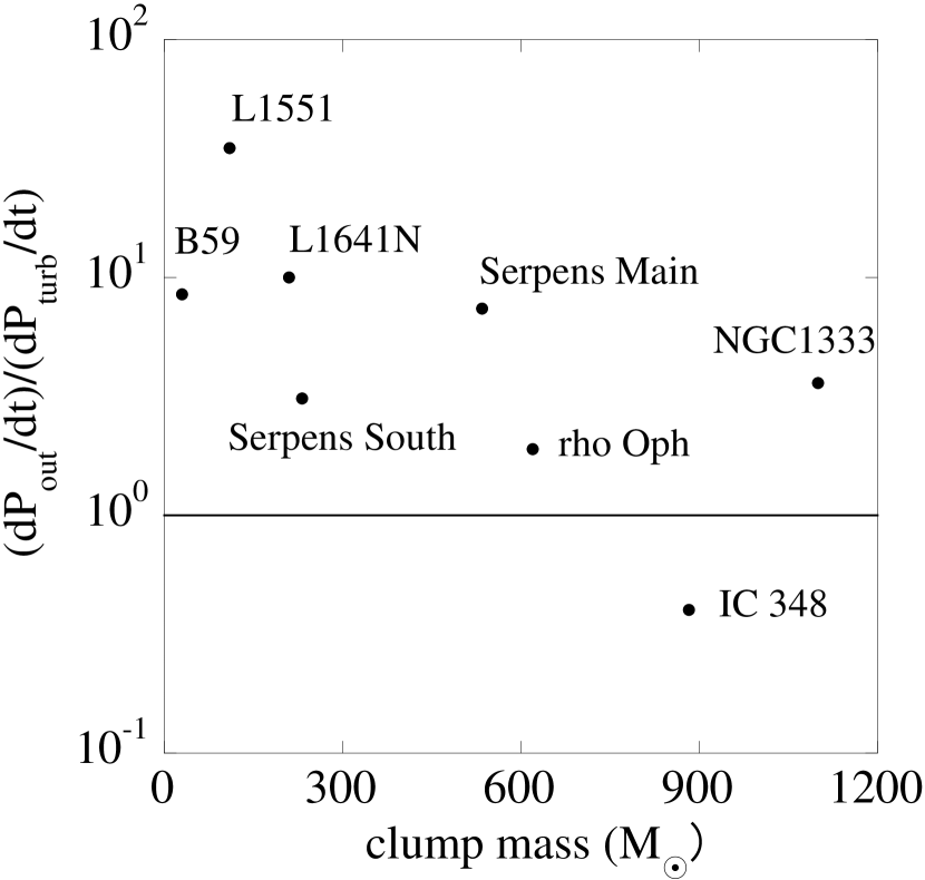
Figure 2: Ratios of the momentum injection to turbulence dissipation rates of nearby cluster-forming clumps as a function of clump mass.

where $\epsilon_{\rm SFR}$ is the star formation rate, and $P_{*}$ the momentum per one solar mass of star formed (Matzner & McKee, 2000), $f_{\rm w}$ the fraction of the outflow that contributes to the generation of molecular outflows, and $f_{\rm out}$ the fraction of the molecular outflow momentum that is converted into the clump internal turbulence momentum. The value $f_{\rm out}$ is uncertain, but is expected to be in the range of 0.1 to 1, following the numerical simulations. According to Figure 2 of Nakamura & Li (2007), the clump with about $10^{3}M_{\odot}$ has reached a quasi-virial equilibrium at the velocity dispersion of about 5 $c_{s}$ in a few clump free-fall times $t_{\rm ff}$, where $c_{s}$ is the isothermal sound speed. The total amount of the specific momentum injected into the clump almost linearly increases with time and reaches about 10 $c_{s}$ in $3t_{\rm ff}$, where the free-fall time is estimated by taking into account the fact that the clump mean density has increased by a factor of a few in a quasi-virial equilibrium state. The outflow momentum injection rate is estimated to be $f_{\rm out}M_{\rm cl}\times 10c_{s}/3t_{\rm ff}$, where we made the approximation that the clump mass is constant because the total mass of stars formed is only a few percent the clump mass. On the other hand, the turbulence dissipation rate is roughly estimated to be $0.21M_{\rm cl}\times 5c_{s}/t_{\rm diss}$ and the dissipation time $t_{\rm diss}$ is comparable to $t_{\rm ff}$. Balancing the momentum injection rate agaist the turbulence dissipation rate yields $f_{\rm out}\sim 0.3$.

The actual value of $f_{\rm out}$ may depend on the mass and size of the clump. For less massive, small clumps, $f_{\rm out}$ may be smaller because the outflow lobes are easier to break out of the clump. The typical outflow speed $V_{W}$ is about $10^{2}$ km s^-1 (e.g., Matzner & McKee, 2000), which is assumed to be constant, independent of the stellar mass. Replacing $\epsilon_{\rm SFR}$ by the star formation rate per free-fall time SFR_ff, Equation (8) is rewritten as

$$\frac{dP_{\rm out}}{dt} = f_{\rm out}{\rm SFR}_{\rm ff}{M_{\rm cl}\over t_{\rm ff}}f_{\rm W}V_{\rm W}$$ (8)

$$\simeq 2.3\times 10^{-4}M_{\odot}{\rm km\ s}^{-1}\ {\rm yr}^{-1}\left(f_{\rm out}\over 0.3\right)\left({{\rm SFR}_{\rm ff}\over 0.01}\right)\left({f_{\rm W}\over 0.4}\right)\left({V_{\rm W}\over 100\ {\rm km\ s}^{-1}}\right)\left({M_{\rm cl}\over 500\ M_{\odot}}\right)^{3/2}\left({R_{\rm cl}\over 0.5\ {\rm pc}}\right)^{-3/2}\ ,$$

where the free-fall time is defined as

$$t_{\rm ff} = \sqrt{3\pi\over 32G\rho}$$ (9)

$$\simeq 0.26\ {\rm Myr}\left({M_{\rm cl}\over 500\ M_{\odot}}\right)^{-1/2}\left({R_{\rm cl}\over 0.5\ {\rm pc}}\right)^{3/2}\ .$$

2.3 Star Formation Rate Per Free-Fall Time

Using Equations (3), (4), (6), and (8), the star formation rate per free-fall time expected from the outflow-regulated cluster formation model is given by

$${\rm SFR}_{\rm ff} \simeq 0.13af_{\rm B}f_{\rm out}f_{\rm w}^{-1}V_{\rm w}^{-1}\frac{GM_{\rm cl}}{R_{\rm cl}^{2}}t_{\rm ff}$$ (10)

$$= 0.02\left(\frac{f_{\rm B}}{0.5}\right)\left(f_{\rm out}\over 0.3\right)^{-1}\left(\frac{f_{\rm w}}{0.4}\right)^{-1}\left(\frac{V_{\rm w}}{10^{2}\ {\rm km\ s^{-1}}}\right)^{-1}\left(\frac{M_{\rm cl}}{500\ M_{\odot}}\right)^{1/2}\left(\frac{R_{\rm cl}}{0.5\ {\rm pc}}\right)^{-1/2}\ .$$

For the fiducial numbers of the physical quantities of nearby cluster-forming clumps, the star formation rate per free-fall time is estimated to be a few percent, implying that the outflow-regulated cluster formation model predicts slow star formation.

If the star formation rate per free-fall time can be estimated from the observations, then the number of protostars formed in a free-fall time, $N$, is given by

$$N \simeq M_{\rm cl}{\rm SFR}_{\rm ff}^{\rm obs}/M_{*}$$ (11)

$$= 10\left({{\rm SFR}_{\rm ff}^{\rm obs}\over 0.01}\right)\left({M_{\rm cl}\over 500\ M_{\odot}}\right)\left({M_{*}\over 0.5\ M_{\odot}}\right)^{-1}\ ,$$

where $M_{*}$ is the mean mass of a protostar assuming the standard stellar IMF and here we adopt $M_{*}\simeq 0.5M_{\odot}$, following Chabrier (2005). Then, the average number of protostars observed at any given time can be estimated as

$$N_{\rm obs}\simeq N{t_{\rm life}\over t_{\rm ff}}\ ,$$ (12)

where $t_{\rm life}$ is the typical lifetime of protostars. Assuming that the protostars are the Class 0/I objects, $t_{\rm life}$ is estimated to be $t_{\rm life}\sim 0.4$ Myr (Evans et al., 2009). From the observed number of Class 0/I objects, we can derive the star formation rate per free-fall time from

$${\rm SFR}_{\rm ff}^{\rm obs}\simeq 0.01\left({N_{\rm obs}\over 20}\right)\left({M_{\rm cl}\over 500\ M_{\odot}}\right)^{-3/2}\left({M_{*}\over 0.5\ M_{\odot}}\right)\left({t_{\rm life}\over 0.4\ {\rm Myr}}\right)^{-1}\left({R_{\rm cl}\over 0.5\ {\rm pc}}\right)^{3/2}\ .$$ (13)

2.4 Dynamical Impact of Protostellar Outflow Feedback

To assess how the outflow feedback influences the clump dynamics, we apply the virial analysis to the cluster-forming clump. The virial equation of a spherical clump is written as

$${1\over 2}\frac{\partial^{2}I}{\partial t^{2}}=2U+W,$$ (14)

where $I$ is the moment of inertia, $U$ is the clump kinetic energy, and $W$ is the clump gravitational energy. The term $U$ and $W$ are given, respectively, by

$$U = {3M_{\rm cl}\sigma_{\rm 1D}^{2}\over 2}$$ (15)

$$= 750M_{\odot}\ {\rm km^{2}\ s}^{-2}\left(M_{\rm cl}\over 500\ M_{\odot}\right)\left(\sigma_{\rm 1D}\over{\rm km\ s}^{-1}\right)^{2}\ ,$$ (16)

and

$$W = -{3\over 5}af_{B}{GM^{2}\over R}$$ (17)

$$\simeq -1075M_{\odot}{\rm km^{2}\ s}^{-2}\left(a\over 5/3\right)\left(f_{B}\over 0.5\right)\left(M_{\rm cl}\over 500\ M_{\odot}\right)^{2}\left(R_{\rm cl}\over 0.5\ {\rm pc}\right)^{-1}\ .$$ (18)

In the outflow-regulated cluster formation model, the clump is in quasi-virial equilibrium, i.e., $\alpha_{\rm vir}\sim 1$, where $\alpha_{\rm vir}$ is the virial parameter defined as

$$\alpha_{\rm vir} \equiv -{2U\over W}={5\sigma_{\rm 1D}^{2}R_{\rm cl}\over af_{B}GM_{\rm cl}}$$ (19)

$$\simeq 1.4\left({a\over 5/3}\right)^{-1}\left(f_{B}\over 0.5\right)^{-1}\left({\sigma_{\rm 1D}\over{\rm km\ s}^{-1}}\right)^{2}\left({R_{\rm cl}\over 0.5\ {\rm pc}}\right)\left({M_{\rm cl}\over 500\ M_{\odot}}\right)^{-1}\ .$$ (20)

If the total outflow kinetic energy, $E_{\rm out}$, is significantly smaller than the clump kinetic and gravitational energies, $U$ and $-$W, then the outflow energy injection contributes little to the clump dynamical state. To evaluate the impact of outflow feedback on the clump dynamics, we introduce the following non-dimensional quantity,

$$\eta_{\rm out}\equiv-{2E_{\rm out}\over W}\ .$$ (21)

If $\eta_{\rm out}$ is as small as $\sim$ 0.1, then the outflow feedback is expected to play only a minor role in the clump dynamics. On the other hand, if $\eta_{\rm out}$ is larger than $\sim 1$, the role of outflow feedback would be much more significant: the clump material is expected to be dispersed away from the parent clump, and subsequent star formation is suppressed.

Here we consider only protostellar outflow feedback as the potential clump disruption mechanism. This limits the clump mass to less than about 3000 M_⊙, above which UV radiation from O stars is likely to dominate the clump destruction assuming the standard stellar IMF and star formation efficiencies (Matzner & McKee, 2000; Matzner, 2002).

3 Confronting Model with Molecular Outflow Surveys

Recently, several extensive molecular outflow surveys using the ¹²CO lines have been carried out toward nearby cluster-forming regions. Here, we compare some characteristics of the outflow-regulated cluster formation model with the survey results toward 8 nearby cluster-forming clumps, (1) B59, (2) L1551, (3) L1641N, (4) Serpens Main Cloud, (5) Serpens South, (6) $\rho$ Oph, (7) IC 348, and (8) NGC 1333. The masses of the clumps range from a few $\times 10M_{\odot}$ to $10^{3}M_{\odot}$. All the cluster-forming clumps have distances smaller than about 400 pc, so that the molecular outflows can be identified in reasonable spatial resolutions even with single-dish telescopes. Since all the clumps contain no massive stars that would emit strong UV radiation, the outflow feedback is expected to be the leading stellar feedback mechanism in these regions.

It is worth noting that Arce et al. (2011) carried out detailed analysis of large-scale ¹³CO ($J=1-0$) mapping data toward the Perseus molecular cloud and found a number of parsec-scale expanding bubbles that are presumably driven by stellar winds from intermediate-mass protostars. These bubbles are also expected to contribute to turbulence driving in the clouds. Similar bubbles are also found in other regions like the Orion A molecular cloud (Heyer et al., 1992; Nakamura et al., 2012)

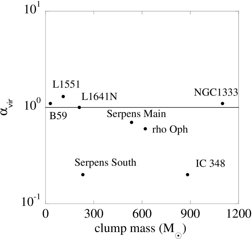
Figure 1: Virial parameters of nearby cluster-forming clumps as a function of clump mass. To estimate the virial parameters, we neglect the possible magnetic support. In this sense, the derived values show lower limits. We note that the physical quantities such as clump masses, sizes, and velocity dispersions are estimated with the ¹³CO ($J=1-0$) data except for Serpens Main and Serpens South. For Serpens Main and Serpens South, the C¹⁸O ($J=1-0$) and N₂H⁺ and Herschel data are used, respectively. See the text for detail.

We present a brief summary of the molecular outflow surveys toward these 8 clumps in Table 1, where the target name, observed ¹²CO transition, telescope, receiver, observed period, velocity resolution ($\Delta V$), effective angular resolution ($\theta_{\rm eff}$), and rms noise level ($\Delta T_{\rm mb}$) are listed. Physical parameters of these clumps derived from the observations are also summarized in Table 2, where the distance assumed, mass, radius, mean surface density, 1D velocity dispersion, clump kinetic energy, gravitational energy, virial parameter, molecular line used, and reference are presented. The masses and radii are rescaled from the values presented in the literature by taking into account the different distances assumed. The virial parameters obtained from the observations are shown as a function of clump mass in Figure 1. For B59, we only consider the central round clump and do not take into account the north-east and U-shape ridges (see Figure 1 of Duarte-Cabral et al. (2012)). We note that all clumps except Serpens Main and Serpens South were observed with the same molecular line tracer ¹³CO, whereas Serpens Main and Serpens South were observed with different molecular line tracers, C¹⁸O and N₂H⁺, respectively. In general, the velocity dispersions derived from these high density tracers are smaller than those derived with ¹³CO. But, its effect is expected to be minor for the estimation of the virial parameters because the clumps are centrally-condensed, and thus the virial parameters are not so sensitive to the density. In fact, for a clump with $\rho\propto r^{-2}$ and constant velocity dispersion, the virial parameter is a constant independent of radius. The other quantities such as $dP_{\rm turb}/dt$, virial velocity, $dP_{\rm out}/dt$ predicted by the model are also constant for all radii when the density distribution follows $\rho\propto r^{-2}$. It is worth noting that for the Serpens South clump, CO appears to be highly depleted (Nishitani et al. 2014, in prep.) and ¹²CO and ¹³CO are significantly self-absorbed. Even the C¹⁸O emission does not follow the dense clump well. So, we adopt the mass estimated from the Spectral Energy Distribution (SED) fitting of the Herschel data (Tanaka et al., 2013), for which the column density is summed up in the area enclosed by a contour line of $5\times 10^{22}$ cm^-2. For all clumps, the virial parameters are also estimated by omitting the effect of magnetic field, i.e., $f_{B}=1$ is assumed.

Table 2 shows that the virial parameters of the clumps are close to unity for all the clumps except for the Serpens South and $\rho$ Oph clumps. This suggests that almost all the clumps are not far from the virial equilibrium. For Serpens South and $\rho$ Oph, the virial parameters are found to be very small, $\alpha_{\rm vir}\sim 0.2$. For the Serpens South clump, Tanaka et al. (2013) found that the infall motions are too slow compared to the free-fall velocity, implying that the magnetic support may play a role in the clump support (see also Sugitani et al., 2011) and therefore we speculate that the “effective” virial parameter including the effect of magnetic support is close to unity. The $\rho$ Oph clump also has a relatively small velocity dispersion, which is much smaller than the free-fall velocity. However, the magnetic field appears not to be spatially well-ordered (Tamura et al., 2011), suggesting that the magnetic field may not be as important for the clump support as in Serpens South. It remains unclear why $\rho$ Oph has a small virial parameter and appears to be relatively quiescent. In fact, only one Class 0 object, VLA1623, is found in the clump. The $\rho$ Oph clump has very high visual extinction (Enoch et al., 2007), which may suggest the presence of foreground molecular gas, or the $\rho$ Oph clump may be elongated along the line-of-sight, which would lead to an under-estimate of the virial parameter and an over-estimate of the angle dispersion of the near IR polarization vectors. The deficiency of Class 0 objects may be due to high extinction or, the star formation activity may be temporarily inactive (Enoch et al., 2009). Either way, the $\rho$ Oph clump is somewhat different from the other cluster-forming clumps in our sample.

In the following, we will use the observational data to address two specific questions that lie at the heart of the outflow-regulated cluster formation model: (1) Does the outflow feedback has enough momentum to supply the dissipated turbulent motions? (2) Is the star formation in the surveyed region fast or slow? In addition, we will try to determine whether the outflow feedback has enough kinetic energy to unbind the parent clump, which is required in the competing model of rapid cluster formation.

3.1 Outflow-Generated Turbulence

In the outflow-regulated cluster formation model, the turbulence momentum dissipation rate should balance the outflow momentum injection rate. In Table 3, we present the turbulence momentum dissipation rate $dP_{\rm turb}/dt$, the outflow momentum injection rate $dP_{\rm out}/dt$, their ratio $(dP_{\rm out}/dt)/(dP_{\rm turb}/dt)$, the outflow momentum, the outflow kinetic energy $E_{\rm out}$, and the ratio $\eta_{\rm out}$ for all 8 cluster-forming clumps. The outflow parameters are derived from the quantities presented in the references shown in Table 1 after applying corrections to account for different distances adopted and different assumptions. To estimate these quantities, we assume the following: (1) the inclination angles of the outflow axes are around $\xi\simeq 57.3^{\circ}$, (2) the outflow material is optically-thin, and (3) the typical dynamical time of the outflows is $3\times 10^{4}$ year. The second assumption leads to an under-estimation of the outflow momentum injection rates and the outflow kinetic energies by a factor of a few or more. Also, the outflow momenta and energies are underestimated at least by a factor of a few because the low-velocity components are omitted due to the difficulty in separating such outflow components from the ambient clump material (Bally et al., 1999; Arce et al., 2010; Offner et al., 2011). For example, for $\rho$ Oph, the emission whose LSR velocity is in the range from 1 km s^-1 to 6.5 km s^-1 is not taken into account in estimating the physical parameters of the outflows, although this velocity width of 5.5 km s^-1 is much larger than the FWHM velocity width of the clump (1.5 km s^-1). For the Serpens Main Cloud and Serpens South, the emissions with 6 km s^-1 $\leq V_{\rm LSR}\leq 10$ km s^-1 and 4 km s^-1 $\leq V_{\rm LSR}\leq 11$ km s^-1 are omitted, respectively, and the velocity widths of 4 km s^-1 and 7 km s^-1 are about twice and 5 times larger than the FWHM velocity widths of 2 km s^-1 and 1.2 km s^-1, respectively. In total, the outflow masses, momenta, and kinetic energies derived from the observations are likely to be underestimated by an order of magnitude. This underestimation of the outflow physical quantities may be compensated by the factor $f_{\rm out}$, which is the fraction of the molecular outflow momentum that is converted into the clump turbulent momentum, and is expected to be around a few $\times 10^{-1}$. Therefore, we assume that the momentum injection rates derived from the observations (presented in Table 3) are comparable to the outflow momentum injection rate. We present the ratio $(dP_{\rm out}/dt)/(dP_{\rm turb}/dt)$ as a function of clump mass in Figure 2.

According to Table 3 and Figure 2, for all clumps except $\rho$ Oph, the outflow momentum injection rate is comparable to or larger than the turbulence dissipation rate. Therefore, we conclude that the outflows can maintain supersonic turbulence in the cluster-forming clumps. For the three least massive clumps, B59, L1551, and L1641N, the ratios between $dP_{\rm out}/dt$ and $dP_{\rm turb}/dt$ tend to be larger. This is presumably due to the fact that these clumps are nearest and the numbers of outflow lobes and protostars are smaller, and thus it is easier to distinguish between the outflow components and ambient clump gas.

We note that in previous studies, the energy dissipation and injection rates are compared to assess whether the outflow feedback can maintain the turbulent motions in the cluster-forming clumps. The main conclusion is that the energy injection rate due to the outflow feedback is generally larger than the energy dissipation rate, and thus the outflow feedback has enough energy to maintain the turbulent motions (e.g., Hatchell et al., 2007; Stanke & Williams, 2007; Swift & Welch, 208; Maury et al., 2009; Arce et al., 2010; Curtis et al., 2010; Nakamura et al., 2011a, b). However, the outflow feedback is a momentum-driven feedback because radiative energy loss is efficient in the clouds and clumps (Fall et al., 2010). Thus, our approach of using the momentum dissipation and injection rates is likely to be more appropriate.

3.2 Dynamical Impact of Outflow Feedback

As shown in Table 2, almost all clumps appear close to virial equilibrium. The outflow feedback should provide additional force in the clump material. If the outflows have enough energies to disperse the surrounding gas, then the outflow feedback can quench further star formation. Here, we measure the dynamical effect of the outflow feedback in the clump destruction, using the non-dimensional parameter $\eta_{\rm out}$, the ratio between 2$E_{\rm out}$ and $-W$.

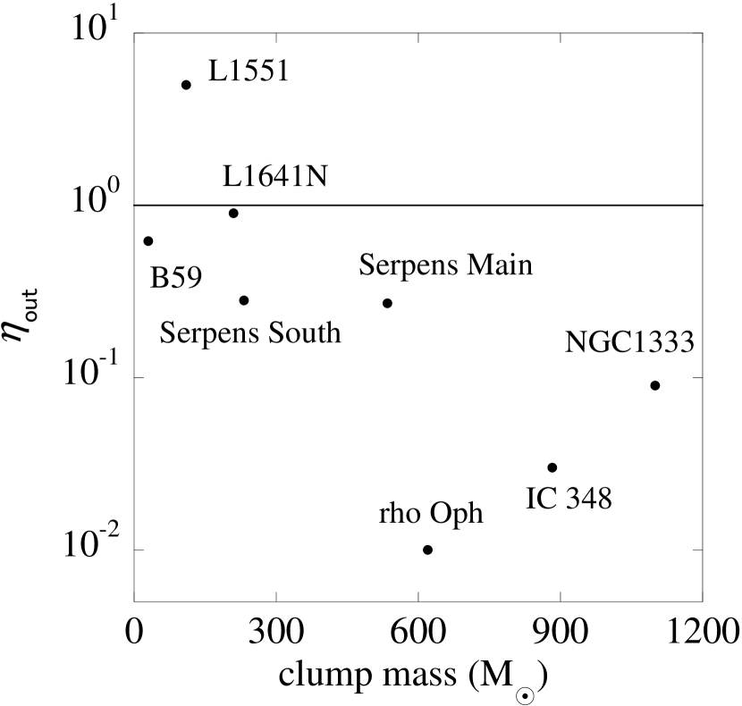
Figure 3: Ratios of twice the outflow kinetic energy $2E_{\rm out}$ to the gravitational binding energy of the clump $-W$, $\eta_{\rm out}$, of nearby cluster-forming clumps as a function of clump mass.

In the last column of Table 3 and Figure 3, we present the values $\eta_{\rm out}$ derived from the observations. We note that presumably only a fraction of $E_{\rm out}$ contributes to the dispersal of the clump material because a significant fraction of the outflow kinetic energy escapes out of the clump once the outflow breaks out. This fraction is expected to be larger for less massive, smaller clumps. However, this effect may be compensated by the fact that the outflow kinetic energies derived from the observations are likely to be underestimated by an order of magnitude. Therefore, we use the values of $\eta_{\rm out}$ presented in Table 3 to assess the dynamical impact of the outflow feedback.

For the three least massive clumps, B59, L1551, and L1641N, the values of $\eta_{\rm out}$ are large, indicating that the outflow feedback has potential to impact the clump structure and dynamics significantly. For L1641N, there is evidence that the stellar feedback may have dispersed the clump material significantly (Reipurth et al., 1998; Nakamura et al., 2012). For the intermediate mass clumps such as the Serpens Main Cloud and Serpens South, the outflow kinetic energy may partly influence the clump dynamical evolution. In contrast, for massive clumps, the outflow feedback appears to play a minor role in the global clump dynamics. In other words, it is likely difficult to destroy the whole clumps only by the current outflow activity. This suggests that whether the outflow feedback can destroy the cluster-forming clumps or not may depend on the clump mass. For massive clumps, the outflow feedback appears unable to disperse the clump material significantly and thus the star formation may proceed a relatively long time.

3.3 Star Formation Rate Per Free-Fall Time

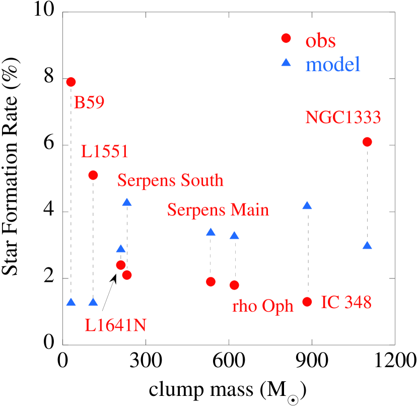
Figure 4: Star formation rates per free-fall time of nearby cluster-forming clumps. The red circles and blue triangles indicate SFR_ff derived from observations and SFR_ff predicted by the outflow-regulated cluster formation model, respectively.

Table 4 summarizes the number of protostars (Class 0 and I objects) observed in the individual clumps, and the star formation rates per free-fall time derived from the observations and Equation (10). The star formation rates per free-fall time derived from the observations and predicted by the model are presented in Figure 4. For B59, L1551, and L1641N, we adopt the results of Brooke et al. (2007), Stojimirovic et al. (2006), and Megeath et al. (2012), respectively. For the Serpens Main Cloud and $\rho$ Oph, the numbers of protostars are calculated using the results of the Spitzer observations (Evans et al., 2009). For Serpens South, we count the protostars located within the circle indicated in Figure 1 of Gutermuth et al. (2008). We also add the Class 0 sources identified within the circle by Bontemps et al. (2010). For IC 348 and NGC 1333, we adopt the numbers shown in Arce et al. (2010). Here, we adopt the typical lifetime for Class I objects of 0.4 Myr on the basis of the results of the Spitzer Gould Belt Survey (Evans et al., 2009), although the lifetime may depend on the interstellar environments somewhat. For all clumps, the observed SFR${}_{\rm ff}^{\rm obs}$ and SFR_ff predicted by the outflow-regulated cluster formation model stays as low as a few percent. Taking into account that the quantities have uncertainty at least by a factor of a few, we conclude that they are consistent with each other, supporting the slow cluster formation model. If SFR${}_{\rm ff}=10\sim$ a few $\times 10$ % as suggested by the rapid cluster formation model, the lifetime of the Class I objects should be of order of $10^{4}$ yr, which is too short (Evans et al., 2009).

4 Conclusion

In the present paper, we constructed an analytic model of the outflow-regulated cluster formation scenario and confronted some of the model predictions with recent outflow surveys toward 8 nearby cluster-forming clumps: B59, L1551, L1641N, Serpens Main Cloud, Serpens South, IC 348, and NGC 1333. We found that the observational results support the outflow-regulated cluster formation model in general. The main conclusions are summarized below.

• We constructed an analytic model of the outflow-regulated cluster formation, in which we assumed that the turbulence dissipation rate is balanced by the outflow momentum injection rate in a cluster-forming clump that is in virial equilibrium. In this model, the star formation rate per free-fall time is predicted to be a few percent.

• Most of the surveyed cluster-forming clumps have virial parameters close to unity, indicating that the internal turbulent motions play an important role in the clump support, and that the clumps are close to virial equilibrium in general. The exceptions are Serpens South and $\rho$ Oph, where the virial parameters are estimated to be as small as $\sim$ 0.2. In Serpens South, Sugitani et al. (2011) revealed the existence of globally-ordered magnetic field that appears to be roughly perpendicular to the main filament, indicating that the magnetic support is important (see also Tanaka et al., 2013). In contrast, for $\rho$ Oph, no globally-ordered magnetic field has been observed (Tamura et al., 2011). However, the clump does not appear to be globally collapsing at the free-fall rate despite its slow internal turbulent motions. It remains unclear why $\rho$ Oph appears relatively quiescent. It might be elongated along the line-of-sight, so that the virial parameter is underestimated.

• For most of the clumps, the outflow momentum injection rate is comparable to or larger than the turbulence momentum dissipation rate. We note that the outflow momenta are underestimated in this paper because the outflow gas is assumed to be optically-thin and the low-velocity outflow components are ignored. The actual outflow momentum injection rates should be larger by a factor of a few or more. Thus, we conclude that the outflow feedback can maintain supersonic turbulence in the surveyed nearby cluster-forming regions.

• However, the outflow kinetic energy is only a fraction of the clump gravitational energy except for the three least massive clumps, B59, L1551 and L1641N. Therefore, we conclude that the outflow feedback is not enough to disperse the whole clump at least for the intermediate-mass and massive clumps.

• Using the numbers of Class 0/I objects, the star formation rates per free-fall time are estimated to be a few percent for all 8 clumps, which is consistent with the outflow-regulated scenario of slow cluster formation.

Table 1: Summary o ¹²CO Outflow Surveys Toward Nearby Parsec-Scale Cluster-Forming Clumps

Name	CO transition	telescope	receiver	period	$\Delta V$	$\Delta\theta_{\rm eff}$	$\Delta T_{\rm mb}$	Referencee
					(km s-1)	(′′)	(K)
B59	$3-2$	JCMT	HARP	2010.5 $-$ 2010.6	0.5	20	0.2	1
L1551	$1-0$	FCRAO	SEQUOIA	2001 $-$ 2002	0.25	50	0.2	2
L1641N	$1-0$	NRO	BEARS	2009.12$-$2010.1	0.5	21	1.2	3
Serpens Main	$3-2$	JCMT	HARP	2007.4, 2007.7	1.0	20	0.16	4
Serpens South	$3-2$	ASTE	MAC 345	2010.8	0.5	24	0.19	5
$\rho$ Oph	$1-0$	NRO	BEARS	2009.12$-$2010.5	0.4	30	1.0	6
IC 348	$1-0$	FCRAO	SEQUOIA	2002$-$2005	0.07	50	0.5	7
NGC1333	$1-0$	FCRAO	SEQUOIA	2002$-$2005	0.07	50	0.5	7

Note. — See Section 3 in detail.

Table 2: Physical Parameters of Nearby Parsec-Scale Cluster-Forming Clumps

Name	Distance	Mass	Radius	$\Sigma$	$\sigma_{\rm 1D}$	$U$	$W$	$\alpha_{\rm vir}$	molecular line	Reference
	(pc)	($M_{\odot}$)	(pc)	(g cm-2)	(km s-1)	($M_{\odot}$ km2s-2)	($M_{\odot}$ km2s-2)
B59	130	30	0.3	0.17	0.4	7	13	1.1	13CO ($1-0$)	1
L1551	140	110	1	0.007	0.45	33	52	1.3	13CO ($1-0$)	2
L1641N	400	210	0.55	0.045	0.74	214	581	1.0	13CO ($1-0$)	3
Serpens Main	415	535	0.73	0.065	0.85	580	1686	0.7	C18O ($1-0$)	4,5
Serpens South	415	232	0.2	0.38	0.53	98	1157	0.2	Herschel, N2H+ ($1-0$)	6
$\rho$ Oph	125	883	0.8	0.090	0.64	543	4191	0.2	13CO ($1-0$)	7
IC 348	250	620	0.9	0.050	0.76	753	1837	0.6	13CO ($1-0$)	8
NGC 1333	250	1100	2.0	0.018	0.93	1427	2602	1.1	13CO ($1-0$)	8

Table 3: Observations of Nearby Parsec-Scale Cluster-Forming Clumps

Name	$dP_{\rm turb}/dt$	$dP_{\rm out}/dt^{a}$	$(dP_{\rm out}/dt)/(dP_{\rm turb}/dt)$	${P}_{\rm out}^{b}$	${E}_{\rm out}^{b}$	${\eta}_{\rm out}$
	($M_{\odot}$ km s-1 yr-1)	($M_{\odot}$ km s-1 yr-1)		($M_{\odot}$ km s-1)	($M_{\odot}$ km2 s-2)
B59	$1.0\times 10^{-5}$	$8.5\times 10^{-5}$	8.5	2.6	4	0.62
L1551	$1.8\times 10^{-5}$	$6.3\times 10^{-4}$	35	19	130	5.0
L1641N	$1.3\times 10^{-4}$	$1.3\times 10^{-3}$	10	80	273	0.9
Serpens Main	$3.4\times 10^{-4}$	$2.5\times 10^{-3}$	7.4	75	445	0.27
Serpens South	$2.1\times 10^{-4}$	$6.5\times 10^{-4}$	3.1	19	165	0.28
$\rho$ Oph	$2.9\times 10^{-4}$	$1.2\times 10^{-4}$	0.4	3.6	61	0.03
IC 348	$2.5\times 10^{-4}$	$4.7\times 10^{-4}$	1.9	14	26	0.01
NGC 1333	$3.0\times 10^{-4}$	$1.1\times 10^{-3}$	3.6	32	119	0.09

Table 4: Star Formation in Nearby Parsec-Scale Cluster-Forming Clumps

Name	$N_{\rm Class0/I}$	SFR${}_{\rm ff}^{\rm obs}$a	SFRffb
		(%)	(%)
B59	4	7.9	1.3
L1551	3	5.1	1.3
L1641N	14	2.4	2.9
Serpens Main	14	1.9	3.4
Serpens South	42	2.1	4.3
$\rho$ Oph	23	1.3	4.2
IC 348	16	1.8	3.3
NGC 1333	40	6.1	3.0

Note. — The lifetime of protostars is assumed to be 0.4 Myr for all the regions.

References

- Allen et al. (2007) Allen, L., Megeath, T., Gutermuth, R., et al. 2007, in Protostars and Planets V, eds. B. Reipurth, D. Jewitt, and K. Keil (University of Arizona Press), p. 361
- Arce et al. (2010) Arce, H. G., Borkin, M. A., Goodman, A. A., Pineda, J. E., & Halle, M. W. 2010, ApJ, 715, 1170
- Arce et al. (2011) Arce, H. G., Borkin, M. A., Goodman, A. A., Pineda, J. E., & Beaumont, C. N. 2011, ApJ, 742, 105
- Bally et al. (1999) Bally, J., Reipurth, B., Lada, C. J., & Billawala, Y. 1999, AJ, 117, 410
- Bontemps et al. (2010) Bontemps, S., André, P., Könyves, V., et al. 2010, A&A, 518, L85
- Brooke et al. (2007) Brooke, T. Y., Huard, T. L., Bourke, T. L. et al. 2007, ApJ, 655, 364
- Carroll et al. (2009) Carroll, J. J., Frank, A., Blackman, E. G., Cunningham, A. J., Quillen, A. C. 2009, ApJ, 695, 1376
- Carroll et al. (2010) Carroll, J. J., Frank, A., & Blackman, E. G. 2010, ApJ, 722, 145
- Chabrier (2005) Chabrier, G. 2005, in the Initial Mass Function 50 years later, (eds. E. Corbelli and F. Palla), 2006, p. 41
- Colin et al. (2013) Colin, P., Vazquez-Semadeni, E.,& Gomez, G. C. 2013, MNRAS, 435, 1701
- Cunningham et al. (2009) Cunningham, A. J., Frank, A., Carroll, J. et al., 2009, ApJ, 692, 816
- Curtis et al. (2010) Curtis, E. I., Ritcher, J. S., Swift, J. J. et al. 2010, MNRAS, 408,1516
- Dib (2011) Dib, S. 2011, ApJ, 737, L20
- Duarte-Cabral et al. (2012) Duarte-Cabral, A., Chrysostomou, A., Peretto, N., et al. 2012, ApJ, 543, 140
- Elmegreen (2007) Elmegreen, B. G. 2007, ApJ, 668, 1064
- Enoch et al. (2007) Enoch, M. L., Glenn, J., Evans, N. J. II et al. 2007, ApJ, 666, 982
- Enoch et al. (2009) Enoch, M. L., Evans, N. J. II, Sargent, A. I., & Glenn, J. 2009, ApJ, 692, 973
- Evans et al. (2009) Evans, N. J. II, Dunham, M. M., Jorgensen, J. K., et al. 2009, ApJS, 181, 321
- Fall et al. (2010) Fall, S. M., Krumholz, M. R., & Matzner, C. D. 2010, ApJ, 710, 142
- Graves et al. (2010) Graves, S. F., Richer, J. S., Buckle, J. V., et al. 2010, MNRAS, 409, 1412
- Gutermuth et al. (2008) Gutermuth, R. A., Bourke, T. L., Allen, L. E., et al. 2008, ApJ, 673, L151
- Hansen et al. (2012) Hansen, C., Klein, R. I., McKee, C. F., Fisher, R. T. 2012, ApJ, 747, 22
- Hartmann & Burkert (2007) Hartmann, L. & Burkert, A. 2007, ApJ, 653, 361
- Hatchell et al. (2007) Hatchell, J., Fuller, G. A., & Richer, J. S. 2007, A&A, 472, 187
- Heyer et al. (1992) Heyer, M. H., Morgan, F. P., Schloerb, R. L., et al. 1992, ApJ, 395, L99
- Krumholz et al. (2006) Krumholz, M. R., Matzner, C. D., & McKee, C. F. 2006, ApJ, 653, 361
- Krumholz et al. (2014) Krumholz, M. R., Bate, M. R., Arce, H. G. et al. 2014, in Protostars and Planets VI, University of Arizona Press (2014), eds. H. Beuther, R. Klessen, C. Dullemond, Th. Henning (arXiv:1401.2473)
- Li & Nakamura (2006) Li, Z.-Y., & Nakamura, F., 2006, ApJ, 640, L187
- Mac Low (1999) Mac Low, M.-M. 1999, ApJ, 524, 169
- Matzner & McKee (2000) Matzner, C. D., & McKee, C. F. 2000, ApJ, 545, 364
- Matzner (2002) Matzner, C. D. 2002, ApJ, 566, 302
- Matzner (2007) Matzner, C. D. ApJ, 2007, 659, 1394
- Maury et al. (2009) Maury A., André, P., & Li, Z.-Y. ApJ, 2009, 499, 175
- Maury et al. (2011) Maury A., André, P., Menshchikov, A., et al. A&A, 2011, 535, 77
- Megeath et al. (2012) Megeath, S. T., Gutermuth, R., Muzerolle, J. et al. 2012, AJ, 144, 192
- McKee & Ostriker (2007) McKee, C. F., & Ostriker, E. C. 2007, ARA&A, 45, 565
- Murray et al. (2010) Murray, N., Quataert, E., & Thompson, T. A. 2010, ApJ, 709, 191
- Nakamura & Li (2007) Nakamura, F., & Li, Z.-Y., 2007, ApJ, 662, 395
- Nakamura & Li (2011) Nakamura, F., & Li, Z.-Y., 2011, ApJ, 740, 36
- Nakamura et al. (2011a) Nakamura, F., Kamada, Y., Kamazaki, T., et al. 2011, ApJ, 726, 46
- Nakamura et al. (2011b) Nakamura, F., Sugitani, K., Shimajiri, Y., et al. 2011, ApJ, 737, 56
- Nakamura et al. (2012) Nakamura, F., Miura, T., Kitamura, Y., et al. 2012, ApJ, 746, 25
- Narayanan et al. (2012) Narayanan, G., Snell, R., Bemis, A. 2012, MNRAS, 425, 2641
- Offner et al. (2011) Offner, S. S. R., Lee, E. J., Goodman, A. A., & Arce, H. 2011, ApJ, 743, 91
- Olmi & Testi (2002) Olmi, L., & Testi, L. 2002, A&A, 392, 1053
- Peters et al. (2010) Peters, T., Klessen, R. S., Mac Low, M.-M., & Banerjee, R. 2010, ApJ, 725, 134P
- Price & Bate (2008) Price, D., & Bate, M. R. 2008, MNRAS, 385, 1820
- Reipurth et al. (1998) Reipurth, B., Devine, D., & Bally, J. 1998, AJ, 116, 1396
- Stojimirovic et al. (2006) Stojimirovic, I., Narayanan, G., Snell, R. L., & Bally, J. 2006, ApJ, 2006, 649, 280
- Stanke & Williams (2007) Stanke, T. & Williams, J. P. 2007, AJ, 133, 1307
- Sugitani et al. (2010) Sugitani, K., Nakamura, F., Tamura, M., et al. 2010, ApJ, 716, 299
- Sugitani et al. (2011) Sugitani, K., Nakamura, F., Watanabe, M., et al. 2011, ApJ, 734, 63
- Swift & Welch (208) Swift, J. J. & Welch, W. J. 2008, ApJS, 174, 202
- Tamura et al. (2011) Tamura, M., Hashimoto, J., Kandori, R., et al., 2011, in Science from Small To Large Telescopes, ASP Conf. Series (eds. P. Bastien, N. Manset, D. P. Clemens, and N. St-Louis), Vol. 449, p. 207
- Tan et al. (2006) Tan, J. C., Krumholz, M. R., & McKee, C. F. 2006, ApJ, 638, 369
- Tanaka et al. (2013) Tanaka, T., Nakamura, F., Awazu, Y. et al. 2013, ApJ, 778, 34
- Tatematsu et al. (1993) Tatematsu, K., Umemoto, T., Murata, Y., et al. 1993, ApJ, 404, 643
- Tilley & Pudritz (2007) Tilley, D. A., & Pudritz, R. E. 2007, MNRAS, 382, 73
- Wang et al. (2010) Wang, P., Li, Z.-Y., Abel, T., & Nakamura, F. 2010, ApJ, 709, 27