A Multigrid Method Based On Shifted-Inverse Power Technique for Eigenvalue Problems

Abstract

A multigrid method is proposed in this paper to solve eigenvalue problems by the finite element method based on the shifted-inverse power iteration technique. With this scheme, solving eigenvalue problem is transformed to a series of nonsingular solutions of boundary value problems on multilevel meshes. Since replacing the difficult eigenvalue solving by the easier solution of boundary value problems, the multigrid way can improve the overall efficiency of the eigenvalue problem solving. Some numerical experiments are presented to validate the efficiency of this new method.

Keywords. Eigenvalue problem, multigrid, shifted-inverse power iteration, finite element method.

AMS subject classifications. 65N30, 65N25, 65L15, 65B99.

1 Introduction

Solving large scale eigenvalue problems becomes a fundamental problem in modern science and engineering society. However, it is always a very difficult task to solve high-dimensional eigenvalue problems which come from physical and chemical sciences. About the solution of eigenvalue problems, [3, 7, 8, 9, 15, 22] and the references cited therein give some types of multigrid schemes which couple the multigrid method with the Rayleigh quotient iteration technique. The involved almost singular linear problems in these methods lead to the numerical unstability. So it is required to design some special solver for these almost singular linear problems [8, 15].

The aim of this paper is to present a type of shifted-inverse power iteration method to solve the eigenvalue problem based on the multigrid technique. Compared with the existed works [3, 7, 8, 15, 22], the method here is a generalization of the Rayleigh quotient iteration technique and does not need to solve the singular linear problems. Recently, we propose another type of multigrid method [17, 18] based on the multilevel correction method [13] which transforms the solution of eigenvalue problem to a series of boundary value problem solving and eigenvalue problem solving in a very coarse space. The proposed method here does not need to solve the eigenvalue problem in the coarse space but needs the eigenvalue problem possessing good eigenvalue separations and the initial approximation having good accuracy. The standard Galerkin finite element method for eigenvalue problems has been extensively investigated, e.g. Babuška and Osborn [1, 2], Chatelin [5] and references cited therein. Here we adopt some basic results in these papers for our analysis. The corresponding error and computational work discussion of the proposed iteration scheme will be analyzed. Based on the analysis, the new method can obtain optimal errors with an optimal computational work when we can solve the associated linear problems with the optimal complexity.

In order to describe our method clearly, we give the following simple Laplace eigenvalue problem to illustrate the main idea in this paper (sections 3 and 4).

Find $(\lambda,u)\in\mathcal{R}\times H_{0}^{1}(\Omega)$ such that

$$\left\{\begin{array}[]{rcl}-\Delta u&=&\lambda u,\quad{\rm in}\ \Omega,\\ u&=&0,\quad\ \ {\rm on}\ \partial\Omega,\\ \int_{\Omega}u^{2}d\Omega&=&1,\end{array}\right.$$ (1.1)

where $\Omega\subset\mathcal{R}^{2}$ is a bounded domain with Lipschitz boundary $\partial\Omega$ and $\Delta$ denotes the Laplace operator.

First, we construct a series of finite element spaces $V_{h_{1}}$, $V_{h_{2}}$, $\cdots$, $V_{h_{n}}$ which are subspaces of $H_{0}^{1}(\Omega)$ and defined on the corresponding series of multilevel meshes $\mathcal{T}_{h_{k}}\ (k=1,2,\cdots n)$ such that $V_{h_{1}}\subset V_{h_{2}}\subset\cdots\subset V_{h_{n}}$ and $h_{k}=h_{k-1}/\beta$ (see, e.g., [4, 6]). Our multigrid algorithm to obtain the approximation of the eigenpairs can be defined as follows (see sections 3 and 4):

1. Solve an eigenvalue problem in the coarsest space $V_{h_{1}}$:

   Find $(\lambda_{h_{1}},u_{h_{1}})\in\mathcal{R}\times V_{h_{1}}$ such that $\|\nabla u_{h_{1}}\|_{0}=1$ and

   $$\int_{\Omega}\nabla u_{h_{1}}\nabla v_{h_{1}}d\Omega = \lambda_{h_{1}}\int_{\Omega}u_{h_{1}}v_{h_{1}}d\Omega,\ \ \ \forall v_{h_{1}}\in V_{h_{1}}.$$

2. Do $k=1,\cdots,n-1$

   • Solve the following auxiliary boundary value problem:

     Find $\widetilde{u}_{h_{k+1}}\in V_{h_{k+1}}$ such that for any $v_{h_{k+1}}\in V_{h_{k+1}}$

     $$\int_{\Omega}\big{(}\nabla\widetilde{u}_{h_{k+1}}\nabla v_{h_{k+1}}-\alpha_{k+1}\widetilde{u}_{h_{k+1}}v_{h_{k+1}}\big{)}d\Omega = \int_{\Omega}u_{h_{k}}v_{h_{k+1}}d\Omega.$$

   • Do the normalization

     $$u_{h_{k+1}} = \frac{\widetilde{u}_{h_{k+1}}}{\|\nabla\widetilde{u}_{h_{k+1}}\|_{0}}$$

     and compute the Rayleigh quotient for $u_{h_{k+1}}$

     $$\lambda_{h_{k+1}} = \frac{\|\nabla u_{h_{k+1}}\|_{0}^{2}}{\|u_{h_{k+1}}\|_{0}^{2}}.$$

   End Do

If, for example, $\lambda_{h_{1}}$ is the approximation for the first eigenvalue of the problem (1.1) at the first step and $\Omega$ is a convex domain, then we can establish the following results by taking a suitable choice of $\alpha_{k+1}$ (see sections 3 and 4 for details)

$$\|\nabla(u-u_{h_{n}})\|_{0}=\mathcal{O}(h_{n}),\ \ \ {\rm and}\ \ \ |\lambda-\lambda_{h_{n}}|=\mathcal{O}(h_{n}^{2}).$$

These two estimates mean that we obtain asymptotically optimal errors.

In this method, we replace solving eigenvalue problem on the finest finite element spaces by solving a series of boundary value problems in the corresponding series of finite element spaces and an eigenvalue problem in the initial finite element space.

An outline of the paper goes as follows. In Section 2, we introduce the finite element method for the eigenvalue problem and give the corresponding basic error estimates. A type of one shifted-inverse power iteration step is given in Section 3. In Section 4, we propose a type of multigrid algorithm for solving the eigenvalue problem based on the shifted-inverse power iteration step. The computational work estimate of the eigenvalue multigrid method is given in Section 5. In Section 6, two numerical examples are presented to validate our theoretical analysis. Some concluding remarks are given in the last section.

2 Discretization by finite element method

In this section, we introduce some notation and error estimates of the finite element approximation for the eigenvalue problem. The letter $C$ (with or without subscripts) denotes a generic positive constant which may be different at its different occurrences through the paper. For convenience, the symbols $\lesssim$, $\gtrsim$ and $\approx$ will be used in this paper. That $x_{1}\lesssim y_{1},x_{2}\gtrsim y_{2}$ and $x_{3}\approx y_{3}$, mean that $x_{1}\leq C_{1}y_{1}$, $x_{2}\geq c_{2}y_{2}$ and $c_{3}x_{3}\leq y_{3}\leq C_{3}x_{3}$ for some constants $C_{1},c_{2},c_{3}$ and $C_{3}$ that are independent of mesh sizes (see, e.g., [19]).

Let $(V,\|\cdot\|)$ be a real Hilbert space with inner product $(\cdot,\cdot)$ and norm $\|\cdot\|$, respectively. Let $a(\cdot,\cdot)$, $b(\cdot,\cdot)$ be two symmetric bilinear forms on $V\times V$ satisfying

$$a(w,v) \lesssim \|w\|\|v\|,\ \ \forall w,v\in V,$$ (2.1)

$$\|w\|^{2} \lesssim a(w,w),\ \ \forall w\in V,$$ (2.2)

$$0 < b(w,w),\ \ \forall 0\neq w\in V.$$ (2.3)

From (2.1) and (2.2), we know that $\|\cdot\|_{a}:=a(\cdot,\cdot)^{1/2}$ and $\|\cdot\|$ are two equivalent norms on $V$. We assume that the norm $\|\cdot\|$ is relatively compact with respect to the norm $\|\cdot\|_{b}:=b(\cdot,\cdot)^{1/2}$ in the sense that any sequence which is bounded in $\|\cdot\|$, one can extract a subsequence which is Cauchy with respect to $\|\cdot\|_{b}$. We shall use $a(\cdot,\cdot)$ and $\|\cdot\|_{a}$, respectively, as the inner product and norm on $V$ in the rest of this paper.

We assume that $V_{h}\subset V$ is a family of finite-dimensional spaces that satisfy the following assumption:

For any $w\in V$

$$\lim_{h\rightarrow 0}\inf_{v_{h}\in V_{h}}\|w-v_{h}\|_{a}=0.$$ (2.4)

Let $P_{h}$ be the finite element projection operator of $V$ onto $V_{h}$ defined by

$$a(w-P_{h}w,v_{h})=0,\ \ \ \forall w\in V,\ \ \forall v_{h}\in V_{h}.$$ (2.5)

Obviously

$$\|P_{h}w\|_{a}\leq\|w\|_{a},\ \ \ \forall w\in V.$$ (2.6)

For any $w\in V$, by (2.4) we have

$$\|w-P_{h}w\|_{a} = o(1),\ \ \ {\rm as}\ h\rightarrow 0.$$ (2.7)

Define $\eta_{a}(h)$ as

$$\eta_{a}(h)=\sup_{f\in V^{\prime},\|f\|_{b}=1}\inf_{v_{h}\in V_{h}}\|Tf-v_{h}\|_{a},$$ (2.8)

where $V^{\prime}$ denotes the dual space of $V$ and the operator $T:V^{\prime}\rightarrow V$ is defined as

$$a(Tf,v) = b(f,v),\ \ \ \forall f\in V^{\prime},\ \ \forall v\in V.$$ (2.9)

In order to derive the error estimate of eigenpair approximation in the weak norm $\|\cdot\|_{b}$, we need the following weak norm error estimate of the finite element projection operator $P_{h}$.

Lemma 2.1.

([2, Lemma 3.3 and Lemma 3.4])

$$\eta_{a}(h)\rightarrow 0,\ \ \ \ {\rm as}\ h\rightarrow 0,$$ (2.10)

and

$$\|w-P_{h}w\|_{b} \lesssim \eta_{a}(h)\|w-P_{h}w\|_{a},\ \ \ \forall w\in V.$$ (2.11)

In our methodology description, we are concerned with the following general eigenvalue problem:

Find $(\lambda,u)\in\mathcal{R}\times V$ such that $a(u,u)=1$ and

$$a(u,v) = \lambda b(u,v),\quad\forall v\in V.$$ (2.12)

For the eigenvalue $\lambda$, there exists the following Rayleigh quotient expression (see, e.g., [1, 2, 21])

$$\lambda=\frac{a(u,u)}{b(u,u)}.$$ (2.13)

From [2, 5], we know the eigenvalue problem (2.12) has an eigenvalue sequence $\{\lambda_{j}\}:$

$$0<\lambda_{1}\leq\lambda_{2}\leq\cdots\leq\lambda_{k}\leq\cdots,\ \ \ \lim_{k\rightarrow\infty}\lambda_{k}=\infty,$$

and the associated eigenfunctions

$$u_{1},u_{2},\cdots,u_{k},\cdots,$$

where $b(u_{i},u_{j})=\delta_{ij}$. In the sequence $\{\lambda_{j}\}$, the $\{\lambda_{j}\}$ are repeated according to their geometric multiplicity.

Let $M(\lambda_{i})$ denote the eigenfunction space corresponding to the eigenvalue $\lambda_{i}$ which is defined by

$$M(\lambda_{i}) = \big{\{}w\in V:w\ {\rm is\ an\ eigenfunction\ of\ (\ref{weak_problem})\ corresponding}$$ (2.14)

$$\ \ \ \ {\rm to}\ \lambda_{i}\big{\}}.$$

From [1, 2], each eigenvalue $\lambda_{i}$ can be defined as follows

$$\lambda_{i} = \inf_{v\in V\atop v\perp M(\lambda_{j})\ {\rm for}\ \lambda_{j}<\lambda_{i}}\frac{a(v,v)}{b(v,v)}.$$

Now, let us define the finite element approximations of the problem (2.12). First we generate a shape-regular decomposition of the computing domain $\Omega\subset\mathcal{R}^{d}\ (d=2,3)$ into triangles or rectangles for $d=2$ (tetrahedrons or hexahedrons for $d=3$). The diameter of a cell $K\in\mathcal{T}_{h}$ is denoted by $h_{K}$. The mesh diameter $h$ describes the maximum diameter of all cells $K\in\mathcal{T}_{h}$. Based on the mesh $\mathcal{T}_{h}$, we can construct a finite element space denoted by $V_{h}\subset V$.

Then we define the approximation for the eigenpair $({\lambda},u)$ of (2.12) by the finite element method as:

Find $(\bar{\lambda}_{h},\bar{u}_{h})\in\mathcal{R}\times V_{h}$ such that $a(\bar{u}_{h},\bar{u}_{h})=1$ and

$$a(\bar{u}_{h},v_{h}) = \bar{\lambda}_{h}b(\bar{u}_{h},v_{h}),\quad\ \ \ \forall v_{h}\in V_{h}.$$ (2.15)

From (2.15), we know the following Rayleigh quotient expression for $\bar{\lambda}_{h}$ holds (see, e.g., [1, 2, 21])

$$\bar{\lambda}_{h} = \frac{a(\bar{u}_{h},\bar{u}_{h})}{b(\bar{u}_{h},\bar{u}_{h})}.$$ (2.16)

Similarly, we know from [2, 5] the eigenvalue problem (2.15) has eigenvalues

$$0<\bar{\lambda}_{1,h}\leq\bar{\lambda}_{2,h}\leq\cdots\leq\bar{\lambda}_{k,h}\leq\cdots\leq\bar{\lambda}_{N_{h},h},$$

and the corresponding eigenfunctions

$$\bar{u}_{1,h},\bar{u}_{2,h},\cdots,\bar{u}_{k,h},\cdots,\bar{u}_{N_{h},h},$$

where $b(\bar{u}_{i,h},\bar{u}_{j,h})=\delta_{ij},1\leq i,j\leq N_{h}$ ($N_{h}$ is the dimension of the finite element space $V_{h}$).

From the minimum-maximum principle (see, e.g., [1, 2]), the following upper bound result holds

$${\lambda}_{i}\leq\bar{\lambda}_{i,h},\ \ \ i=1,2,\cdots,N_{h}.$$

Similarly, let $M_{h}(\lambda_{i})$ denote the approximate eigenfunction space corresponding to the eigenvalue $\lambda_{i}$ which is defined by

$$M_{h}(\lambda_{i}) = \big{\{}w_{h}\in V_{h}:w_{h}\ {\rm is\ an\ eigenfunction\ of\ (\ref{weak_problem_Discrete})}$$ (2.17)

$$\ \ \ \ {\rm corresponding\ to}\ \lambda_{i}\big{\}}.$$

From [1, 2], each eigenvalue $\lambda_{i,h}$ can be defined as follows

$$\lambda_{i,h} = \inf_{v_{h}\in V_{h}\atop v_{h}\perp M_{h}(\lambda_{j})\ {\rm for}\ \lambda_{j}<\lambda_{i}}\frac{a(v_{h},v_{h})}{b(v_{h},v_{h})}.$$ (2.18)

Then we define

$$\delta_{h}(\lambda_{i})=\sup_{w\in M(\lambda_{i}),\|w\|_{a}=1}\inf_{v_{h}\in V_{h}}\|w-v_{h}\|_{a}.$$ (2.19)

For the analysis in this paper, we introduce the spectral projection as follows [2]:

$$\Pi_{1,h} = \frac{1}{2\pi{\rm i}}\int_{\Gamma}\big{(}z-P_{h}T\big{)}^{-1}dz,$$ (2.20)

where $\Gamma$ is a Jordan curve in $\mathcal{C}$ that encloses the eigenvalue $\lambda_{1}$ and no other eigenvalues.

For the eigenpair approximations by finite element method, there exist the following error estimates.

Proposition 2.1.

([1, Lemma 3.7, (3.29b)], [2, P. 699] and [5])

(i) For any eigenfunction approximation $\bar{u}_{i,h}$ of (2.15) $(i=1,2,\cdots,N_{h})$, there is an eigenfunction $u_{i}$ of (2.12) corresponding to $\lambda_{i}$ such that $\|u_{i}\|_{a}=1$ and

$$\|u_{i}-\bar{u}_{i,h}\|_{a} \leq C\delta_{h}(\lambda_{i}).$$ (2.21)

Furthermore,

$$\|u_{i}-\bar{u}_{i,h}\|_{b}\leq C\eta_{a}(h)\|u_{i}-\bar{u}_{i,h}\|_{a}.$$ (2.22)

(ii) For each eigenvalue, we have

$$\lambda_{i}\leq\bar{\lambda}_{i,h}\leq\lambda_{i}+C\delta_{h}^{2}(\lambda_{i}).$$ (2.23)

Here and hereafter $C$ is some constant depending on $\lambda_{i}$ but independent of the mesh size $h$.

3 One shifted-inverse power iteration step with multigrid method

In this section, we present a type of one shifted-inverse power iteration step to improve the accuracy of the given eigenvalue and eigenfunction approximations. This iteration method only contains solving auxiliary boundary value problems in the finer finite element space.

To analyze our method, we introduce the error expansion of the eigenvalue by the Rayleigh quotient formula which comes from [1, 2, 14, 21].

Lemma 3.1.

([1, 2, 14, 21]) Assume $(\lambda,u)$ is a true solution of the eigenvalue problem (2.12) and $0\neq\psi\in V$. Let us define

$$\widehat{\lambda}=\frac{a(\psi,\psi)}{b(\psi,\psi)}.$$ (3.1)

Then we have

$$\widehat{\lambda}-\lambda = \frac{a(u-\psi,u-\psi)}{b(\psi,\psi)}-\lambda\frac{b(u-\psi,u-\psi)}{b(\psi,\psi)}.$$ (3.2)

For simplicity, here we only state the numerical method for the first eigenvalue $\lambda_{1}$. Assume we have obtained an eigenpair approximation $(\lambda_{1,h_{k}},u_{1,h_{k}})\in\mathcal{R}\times V_{h_{k}}$ with $\|u_{1,h_{k}}\|_{a}=1$. Now we introduce a type of iteration step to improve the accuracy of the current eigenpair approximation $(\lambda_{1,h_{k}},u_{1,h_{k}})$. Let $V_{h_{k+1}}\subset V$ be a finer finite element space such that $V_{h_{k}}\subset V_{h_{k+1}}$. Based on this finer finite element space, we define the following one shifted-inverse power iteration step.

Algorithm 3.1.

One Shifted-inverse Power Iteration Step

1. Solve the following boundary value problem:

   Find $\widehat{u}_{1,h_{k+1}}\in V_{h_{k+1}}$ such that for any $v_{h_{k+1}}\in V_{h_{k+1}}$

   $$a(\widehat{u}_{1,h_{k+1}},v_{h_{k+1}})-\alpha_{1,k+1}b(\widehat{u}_{1,h_{k+1}},v_{h_{k+1}})=b(u_{1,h_{k}},v_{h_{k+1}}).$$ (3.3)

2. Do the normalization for $\widehat{u}_{1,h_{k+1}}$ as

   $$u_{1,h_{k+1}}=\frac{\widehat{u}_{1,h_{k+1}}}{\|\widehat{u}_{1,h_{k+1}}\|_{a}}$$ (3.4)

   and compute the Rayleigh quotient for $u_{1,h_{k+1}}$

   $$\lambda_{1,h_{k+1}} = \frac{a(u_{1,h_{k+1}},u_{1,h_{k+1}})}{b(u_{1,h_{k+1}},u_{1,h_{k+1}})}.$$ (3.5)

Then we obtain a new eigenpair approximation $(\lambda_{1,h_{k+1}},u_{1,h_{k+1}})\in\mathcal{R}\times V_{h_{k+1}}$. Summarize the above two steps into

$$(\lambda_{1,h_{k+1}},u_{1,h_{k+1}})={\it Correction}(\alpha_{1,k+1},u_{1,h_{k}},V_{h_{k+1}}).$$

Theorem 3.1.

When $\alpha_{1,k+1}\neq\bar{\lambda}_{1,h_{k+1}}$ and $\alpha_{1,k+1}<\bar{\lambda}_{2,h_{k+1}}$, after one correction step, the resultant approximation $u_{1,h_{k+1}}\in V_{h_{k+1}}$ has the following error estimates

$$\|u_{1,h_{k+1}}-\Pi_{1,h_{k+1}}u_{1,h_{k+1}}\|_{a} \leq \frac{\theta_{1,k+1}\|u_{1,h_{k}}-\Pi_{1,h_{k+1}}u_{1,h_{k}}\|_{a}}{1-(1+\theta_{1,k+1})\|u_{1,h_{k}}-\Pi_{1,h_{k+1}}u_{1,h_{k}}\|_{a}},$$ (3.6)

where

$$\theta_{1,k+1} = \frac{|\bar{\lambda}_{1,h_{k+1}}-\alpha_{1,k+1}|}{\bar{\lambda}_{2,h_{k+1}}-\alpha_{1,k+1}}.$$ (3.7)

Proof.

Let us define $\gamma=\bar{\lambda}_{1,h_{k+1}}-\alpha_{1,k+1}$, $\widetilde{u}_{1,h_{k+1}}=\gamma\widehat{u}_{1,h_{k+1}}$ and $w_{h_{k+1}}:=\widetilde{u}_{1,h_{k+1}}-\Pi_{1,h_{k+1}}u_{1,h_{k}}$. Then we know

$$a(\widetilde{u}_{1,h_{k+1}},v_{h_{k+1}})-\alpha_{1,k+1}b(\widetilde{u}_{1,h_{k+1}},v_{h_{k+1}})=\gamma b(u_{1,h_{k}},v_{h_{k+1}}),\ \forall v_{h_{k+1}}\in V_{h_{k+1}}.$$ (3.8)

From $u_{1,h_{k}}-\Pi_{1,h_{k+1}}u_{1,h_{k}}\perp M_{h_{k+1}}(\lambda_{1})$, $\Pi_{1,h_{k+1}}u_{1,h_{k}}\in M_{h_{k+1}}(\lambda_{1})$, (3.8) and for any $v_{h_{k+1}}\in V_{h_{k+1}}$

$$a(\Pi_{1,h_{k+1}}u_{1,h_{k}},v_{h_{k+1}})-\alpha_{1,k+1}b(\Pi_{1,h_{k+1}}u_{1,h_{k}},v_{h_{k+1}})=\gamma b(\Pi_{1,h_{k+1}}u_{1,h_{k}},v_{h_{k+1}}),$$ (3.9)

we have $w_{h_{k+1}}\perp M_{h_{k+1}}(\lambda_{1})$ and $a(w_{h_{k+1}},\Pi_{1,h_{k+1}}u_{1,h_{k}})=0$.

From (2.18), (3.8) and (3.9), the following estimates hold

$$\|w_{h_{k+1}}\|_{a}^{2} = \alpha_{1,k+1}b(w_{h_{k+1}},w_{h_{k+1}})+\gamma b(u_{1,h_{k}}-\Pi_{1,h_{k+1}}u_{1,h_{k}},w_{h_{k+1}})$$

$$\leq \frac{\alpha_{1,k+1}}{\bar{\lambda}_{2,h_{k+1}}}\|w_{h_{k+1}}\|_{a}^{2}+|\gamma|\|u_{1,h_{k}}-\Pi_{1,h_{k+1}}u_{1,h_{k}}\|_{b}\|w_{h_{k+1}}\|_{b}$$

$$\leq \frac{\alpha_{1,k+1}}{\bar{\lambda}_{2,h_{k+1}}}\|w_{h_{k+1}}\|_{a}^{2}+\frac{|\gamma|}{\bar{\lambda}_{2,h_{k+1}}}\|u_{1,h_{k}}-\Pi_{1,h_{k+1}}u_{1,h_{k}}\|_{a}\|w_{h_{k+1}}\|_{a}.$$

Then we have

$$\|w_{h_{k+1}}\|_{a} \leq \frac{\bar{|\lambda}_{1,h_{k+1}}-\alpha_{1,k+1}|}{\bar{\lambda}_{2,h_{k+1}}-\alpha_{1,k+1}}\|u_{1,h_{k}}-\Pi_{1,h_{k+1}}u_{1,h_{k}}\|_{a}.$$ (3.10)

From (3.10), $\|u_{1,h_{k}}\|_{a}=1$ and $\widetilde{u}_{1,h_{k+1}}=u_{1,h_{k}}+\Pi_{1,h_{k+1}}u_{1,h_{k}}-u_{1,h_{k}}+\widetilde{u}_{1,h_{k+1}}-\Pi_{1,h_{k+1}}u_{1,h_{k}}$, the following estimates hold

$$\|\widetilde{u}_{1,h_{k+1}}\|_{a} \geq \|u_{1,h_{k}}\|_{a}-\|\Pi_{1,h_{k+1}}u_{1,h_{k}}-u_{1,h_{k}}\|_{a}-\|\widetilde{u}_{1,h_{k+1}}-\Pi_{1,h_{k+1}}u_{1,h_{k}}\|_{a}$$ (3.11)

$$\geq 1-(1+\theta_{1,k+1})\|u_{1,h_{k}}-\Pi_{1,h_{k+1}}u_{1,h_{k}}\|_{a}.$$

Then we have

$$\frac{1}{\|\widetilde{u}_{1,h_{k+1}}\|_{a}} \leq \frac{1}{1-(1+\theta_{1,k+1})\|u_{1,h_{k}}-\Pi_{1,h_{k+1}}u_{1,h_{k}}\|_{a}}.$$ (3.12)

Since $u_{1,h_{k+1}}=\widetilde{u}_{1,h_{k+1}}/\|\widetilde{u}_{1,h_{k+1}}\|_{a}$ and $w_{h_{k+1}}\perp M_{h_{k+1}}(\lambda_{1})$, the following estimates hold

$$\|u_{1,h_{k+1}}-\Pi_{1,h_{k+1}}u_{1,h_{k+1}}\|_{a} = \frac{\|\widetilde{u}_{1,h_{k+1}}-\Pi_{1,h_{k+1}}u_{1,h_{k}}\|_{a}}{\|\widetilde{u}_{1,h_{k+1}}\|_{a}}$$ (3.13)

$$\leq \frac{\theta_{1,k+1}\|u_{1,h_{k}}-\Pi_{1,h_{k+1}}u_{1,h_{k}}\|_{a}}{1-(1+\theta_{1,k+1})\|u_{1,h_{k}}-\Pi_{1,h_{k+1}}u_{1,h_{k}}\|_{a}},$$

which means we have obtained the desired result (3.6) and the proof is complete.. ∎

Remark 3.1.

Let us discuss two choices of $\alpha_{1,k+1}$.

1. If $\alpha_{1,{k+1}}=0$, i.e. we do not use shift, actually Algorithm 3.1 is just to repeat the well-known two grid method [21]. From (3.6), we have

   $$\|u_{1,{h_{k+1}}}-\Pi_{1,h_{k+1}}u_{1,{h_{k+1}}}\|_{a}\leq\kappa_{1,k+1}\|u_{1,{h_{k}}}-\Pi_{1,h_{k+1}}u_{1,h_{k}}\|_{a},$$ (3.14)

   where

   $$\kappa_{1,k+1} = \frac{\frac{\bar{\lambda}_{1,h_{k+1}}}{\bar{\lambda}_{2,h_{k+1}}}}{1-\Big{(}1+\frac{\bar{\lambda}_{1,h_{k+1}}}{\bar{\lambda}_{2,h_{k+1}}}\Big{)}\|u_{1,{h_{k}}}-\Pi_{1,h_{k+1}}u_{1,h_{k}}\|_{a}}.$$

   This indicates that the two grid step has linear convergence speed rate when $\|u_{1,{h_{k}}}-\Pi_{1,h_{k+1}}u_{1,h_{k}}\|_{a}$ is small enough. But if the gap between $\bar{\lambda}_{1,h_{k+1}}$ and $\bar{\lambda}_{2,h_{k+1}}$ is small, the convergence is slow.

2. From Lemma 3.1, the following estimate holds

   $$\lambda_{1,h_{k}}-\bar{\lambda}_{1,h_{k+1}}$$

   $$= \frac{a(\Pi_{1,h_{k+1}}u_{1,h_{k}}-u_{1,h_{k}},\Pi_{1,h_{k+1}}u_{1,h_{k}}-u_{1,h_{k}})}{b(u_{1,h_{k}},u_{1,h_{k}})}$$

   $$\ \ \ \ -\bar{\lambda}_{1,h_{k+1}}\frac{b(\Pi_{1,h_{k+1}}u_{1,h_{k}}-u_{1,h_{k}},\Pi_{1,h_{k+1}}u_{1,h_{k}}-u_{1,h_{k}})}{b(u_{1,h_{k}},u_{1,h_{k}})}$$

   $$\lesssim \|u_{1,h_{k}}-\Pi_{1,h_{k+1}}u_{1,h_{k}}\|^{2}_{a}.$$

   If $\alpha_{1,h_{k+1}}=\lambda_{1,h_{k}}$, from (3.6), we have

   $$\|u_{1,h_{k+1}}-\Pi_{1,h_{k+1}}u_{1,h_{k+1}}\|_{a}\lesssim\|u_{1,h_{k}}-\Pi_{1,h_{k+1}}u_{1,h_{k}}\|^{3}_{a},$$ (3.15)

   which means that the Rayleigh quotient iteration has cubic convergence rate.

The suitable choice for $\alpha_{1,k+1}$ sometimes is not so easy to obtain, since it depends on $\bar{\lambda}_{1,h_{k+1}}$ and $\bar{\lambda}_{2,h_{k+1}}$ which are unknown. But from (3.6), if

$$0<\frac{|\bar{\lambda}_{1,h_{k+1}}-\alpha_{1,k+1}|}{\bar{\lambda}_{2,h_{k+1}}-\alpha_{1,k+1}}<1,$$

the accuracy for the solution of (3.3) can be improved through more times iteration. Then we can design the following modified one multi shifted-inverse power iteration step.

Algorithm 3.2.

Multi Shifted-inverse Power Iteration Step

1. Set $u_{1,h_{k+1}}^{0}=u_{1,h_{k}}$.

2. Do $j=0,\cdots,\ell-1$

   • Solve the following boundary value problem:

     Find $\widehat{u}_{1,h_{k+1}}^{j+1}\in V_{h_{k+1}}$ such that for any $v_{h_{k+1}}\in V_{h_{k+1}}$

     $$a(\widehat{u}_{1,h_{k+1}}^{j+1},v_{h_{k+1}})-\alpha_{1,k+1}^{j+1}b(\widehat{u}_{1,h_{k+1}}^{j+1},v_{h_{k+1}})=b(u_{1,h_{k+1}}^{j},v_{h_{k+1}}).$$ (3.16)

   • Normalize $\widehat{u}_{1,h_{k+1}}^{j+1}$ by

     $$u_{1,h_{k+1}}^{j+1}=\frac{\widehat{u}_{1,h_{k+1}}^{j+1}}{\|\widehat{u}_{1,h_{k+1}}^{j+1}\|_{a}}$$

     and compute the Rayleigh quotient for $u_{1,h_{k+1}}^{j+1}$

     $$\lambda_{1,h_{k+1}}^{j+1}=\frac{a(u_{1,h_{k+1}}^{j+1},u_{1,h_{k+1}}^{j+1})}{b(u_{1,h_{k+1}}^{j+1},u_{1,h_{k+1}}^{j+1})}.$$ (3.17)

   End Do

3. Set $u_{1,h_{k+1}}=u_{1,h_{k+1}}^{\ell}$ and $\lambda_{1,h_{k+1}}=\lambda_{1,h_{k+1}}^{\ell}$.

Then we obtain a new eigenpair approximation $(\lambda_{1,h_{k+1}},u_{1,h_{k+1}})\in\mathcal{R}\times V_{h_{k+1}}$. Summarize the above two steps into

$$(\lambda_{1,h_{k+1}},u_{1,h_{k+1}})={\it Correction}(\{\alpha_{1,k+1}^{j}\}_{j=1}^{\ell},u_{1,h_{k}},V_{h_{k+1}}).$$

In Algorithm 3.2, we can adjust $\ell$ such that the following estimate satisfies

$$\|u_{1,h_{k+1}}-\Pi_{1,h_{k+1}}{u}_{1,h_{k+1}}\|_{a}<\frac{1}{\beta}\|u_{1,h_{k}}-\Pi_{1,h_{k+1}}{u}_{1,h_{k}}\|_{a},$$ (3.18)

where $\beta$ is a constant defined in the following section. In fact, $\ell$ can be very small ($\ell=2$ or $3$) and the modified iteration step makes the choice of $\alpha_{1,k+1}$ become not so sharp as in Algorithm 3.1 and it improves the stability of the iteration step.

4 Multigrid scheme for the eigenvalue problem

In this section, we introduce a type of multigrid scheme based on the One Shifted-inverse Power Iteration Step defined in Algorithm 3.1 or 3.2. This type of multigrid method can obtain the optimal error estimate as same as solving the eigenvalue problem directly in the finest finite element space.

In order to do multigrid scheme, we define a sequence of triangulations $\mathcal{T}_{h_{k}}$ of $\Omega$ determined as follows. Suppose $\mathcal{T}_{h_{1}}$ is given and let $\mathcal{T}_{h_{k}}$ be obtained from $\mathcal{T}_{h_{k-1}}$ via regular refinement (produce $\beta^{d}$ subelements) such that

$$h_{k}=\frac{1}{\beta}h_{k-1}.$$

Based on this sequence of meshes, we construct the corresponding linear finite element spaces such that

$$V_{h_{1}}\subset V_{h_{2}}\subset\cdots\subset V_{h_{n}},$$ (4.1)

and the following relation of approximation errors hold

$$\eta_{a}(h_{k})\approx\frac{1}{\beta}\eta_{a}(h_{k-1}),\ \ \ \ \delta_{h_{k}}(\lambda)\approx\frac{1}{\beta}\delta_{h_{k-1}}(\lambda),\ \ \ k=2,\ldots,n.$$ (4.2)

From the spectral projection definition by (2.20), we have

$$\|\Pi_{1,h_{k}}u_{1,h_{k}}-\Pi_{1,h_{k+1}}u_{1,h_{k}}\|_{a} \leq C_{4}\delta_{h_{k}}(\lambda_{1}),\ \ k=1,\ldots,n-1,$$ (4.3)

where the constant $C_{4}$ is independent of the mesh size $h_{k}$.

Algorithm 4.1.

Eigenvalue Multigrid Scheme

1. Construct a series of nested finite element spaces $V_{h_{1}},V_{h_{2}},\cdots,V_{h_{n}}$ such that (4.1) and (4.2) hold.

2. Solve the following eigenvalue problem:

   Find $(\lambda_{1,h_{1}},u_{1,h_{1}})\in\mathcal{R}\times V_{h_{1}}$ such that $a(u_{1,h_{1}},u_{1,h_{1}})=1$ and

   $$a(u_{1,h_{1}},v_{h_{1}}) = \lambda_{1,h_{1}}b(u_{1,h_{1}},v_{h_{1}}),\ \ \ \ \forall v_{h_{1}}\in V_{h_{1}}.$$ (4.4)

3. Do $k=1,\cdots,n-1$

   Obtain a new eigenpair approximation $(\lambda_{1,h_{k+1}},u_{1,h_{k+1}})\in\mathcal{R}\times V_{h_{k+1}}$ by a correction step

   $$(\lambda_{1,h_{k+1}},u_{1,h_{k+1}})=Correction(\alpha_{1,k+1},u_{1,h_{k}},V_{h_{k+1}}).$$ (4.5)

   End Do

Finally, we obtain an eigenpair approximation $(\lambda_{1,h_{n}},u_{1,h_{n}})\in\mathcal{R}\times V_{h_{n}}$.

For simplicity in this paper, we assume the following estimates hold

$$\eta_{a}(h_{k})\approx h_{k},\ \ \ \ \delta_{h_{k}}(\lambda_{1})\approx h_{k},\ \ \ \ k=1,\ldots,n.$$ (4.6)

Theorem 4.1.

After implementing Algorithm 4.1, the resultant eigenpair approximation $(\lambda_{1,h_{n}},u_{1,h_{n}})$ has the following error estimates

$$\|u_{1,h_{n}}-\Pi_{1,h_{n}}u_{1,h_{n}}\|_{a} \leq C_{5}\delta_{h_{n}}(\lambda_{1}),$$ (4.7)

$$|\lambda_{1,h_{n}}-\bar{\lambda}_{1,h_{n}}| \leq C_{5}\delta_{h_{n}}^{2}(\lambda_{1}),$$ (4.8)

when the mesh size $h_{1}$ is small enough and $\alpha_{1,{k+1}}$ is chosen as follows

$$\alpha_{1,k+1}=\max\left\{0,\frac{2(1+C_{4}/C_{5})\beta\lambda_{1,h_{k}}-\lambda_{2,h_{1}}}{2(1+C_{4}/C_{5})\beta-1}\right\},\ \ \ k=1,\ldots,n-1,$$ (4.9)

where $C_{5}$ is a constant not less than the constant $C$ in (2.21).

Then there exists a constant $C_{6}$ such that the following final convergence results hold

$$\|u_{1}-u_{1,h_{n}}\|_{a} \leq C_{6}\delta_{h_{n}}(\lambda_{1}),$$ (4.10)

$$|\lambda_{1}-\lambda_{1,h_{n}}| \leq C_{6}\delta_{h_{n}}^{2}(\lambda_{1}).$$ (4.11)

Proof.

First, it is obvious that $2(1+C_{4}/C_{5})\beta>1$. If we choose the $\alpha_{1,k+1}$ as in (4.9) and $2(1+C_{4}/C_{5})\beta\lambda_{1,h_{k}}-\lambda_{2,h_{1}}>0$, then $\alpha_{1,k+1}=\frac{2(1+C_{4}/C_{5})\beta\lambda_{1,h_{k}}-\lambda_{2,h_{1}}}{2(1+C_{4}/C_{5})\beta-1}$ and the following estimates hold

$$\theta_{1,k+1} = \frac{|\bar{\lambda}_{1,h_{k+1}}-\alpha_{1,k+1}|}{\bar{\lambda}_{2,h_{k+1}}-\alpha_{1,k+1}}$$ (4.12)

$$= \frac{|\lambda_{2,h_{1}}-\bar{\lambda}_{1,h_{k+1}}+2(1+C_{4}/C_{5})\beta(\bar{\lambda}_{1,h_{k+1}}-\lambda_{1,h_{k}})|}{2(1+C_{4}/C_{5})\beta(\bar{\lambda}_{2,h_{k+1}}-\lambda_{1,h_{k}})+\lambda_{2,h_{1}}-\bar{\lambda}_{2,h_{k+1}}}$$

$$= \frac{1}{2(1+C_{4}/C_{5})\beta}+\mathcal{O}(h_{1}^{2}).$$

If we choose $\alpha_{1,k+1}$ as in (4.9) and $2(1+C_{4}/C_{5})\beta\lambda_{1,h_{k}}-\lambda_{2,h_{1}}<0$, then $\alpha_{1,k+1}=0$ and we have

$$\theta_{1,k+1}=\frac{|\bar{\lambda}_{1,h_{k+1}}-\alpha_{1,k+1}|}{\bar{\lambda}_{2,h_{k+1}}-\alpha_{1,k+1}} = \frac{|\lambda_{1,h_{k}}+(\bar{\lambda}_{1,h_{k+1}}-\lambda_{1,h_{k}})|}{\lambda_{2,h_{1}}+\bar{\lambda}_{2,h_{k+1}}-\lambda_{2,h_{1}}}$$ (4.13)

$$= \frac{1}{2(1+C_{4}/C_{5})\beta}+\mathcal{O}(h_{1}^{2}).$$

Now, let us prove (4.7) by the method of induction. First, it is obvious that (4.7) holds for $n=1$. Then we assume that (4.7) holds for $n=k$. It means we have the following estimate

$$\|u_{1,h_{k}}-\Pi_{1,h_{k}}u_{1,h_{k}}\|_{a} \leq C_{5}\delta_{h_{k}}(\lambda_{1}).$$ (4.14)

Now let us consider the case of $n=k+1$. Combining (4.3), (4.14) and the triangle inequality leads to the following estimates

$$\|u_{1,h_{k}}-\Pi_{1,h_{k+1}}u_{1,h_{k}}\|_{a} \leq \|u_{1,h_{k}}-\Pi_{1,h_{k}}u_{1,h_{k}}\|_{a}+\|\Pi_{1,h_{k}}u_{1,h_{k}}-\Pi_{1,h_{k+1}}u_{1,h_{k}}\|_{a}$$ (4.15)

$$\leq \|u_{1,h_{k}}-\Pi_{1,h_{k}}u_{1,h_{k}}\|_{a}+C_{4}\delta_{h_{k}}(\lambda_{1})$$

$$\leq C_{5}\Big{(}1+\frac{C_{4}}{C_{5}}\Big{)}\delta_{h_{k}}(\lambda_{1}).$$

From (3.7), (4.12)-(4.13) and (4.15), we have

$$\frac{\theta_{1,k+1}}{1-(1+\theta_{1,k+1})\|u_{1,h_{k}}-\Pi_{1,h_{k+1}}u_{1,h_{k}}\|_{a}} = \frac{1}{2(1+C_{4}/C_{5})\beta}+\mathcal{O}(h_{1})$$ (4.16)

$$< \frac{1}{(1+C_{4}/C_{5})\beta},$$

when $h_{1}$ is small enough.

From Theorem 3.1, (4.15) and (4.16), we have

$$\|u_{1,h_{k+1}}-\Pi_{1,h_{k+1}}u_{1,h_{k+1}}\|_{a} \leq \frac{C_{5}}{\beta}\delta_{h_{k}}(\lambda_{1})=C_{5}\delta_{h_{k+1}}(\lambda_{1}).$$ (4.17)

This means that the result (4.7) also holds for $n=k+1$. Thus we prove the desired result (4.7). From Lemma 3.1 and (4.7), we can obtain the desired result (4.8). Finally, (4.10) and (4.11) can be proved from (4.7), (4.8) and the triangle inequality. ∎

Remark 4.1.

We also investigate the condition of the boundary value problem with different choices of $\alpha_{1,k+1}$. If we choose $\alpha_{1,k+1}$ as (4.9) and $2(1+C_{4}/C_{5})\beta\lambda_{1,h_{k}}-\lambda_{2,h_{1}}>0$, then $\alpha_{1,k+1}<\bar{\lambda}_{1,h_{k+1}}$ when the mesh size $h_{1}$ is small enough. It means that (3.3) is a symmetric positive definite linear equation and its condition has the following estimates

$$\frac{\bar{\lambda}_{n,h_{k+1}}-\alpha_{1,k+1}}{\bar{\lambda}_{1,h_{k+1}}-\alpha_{1,k+1}}\approx\frac{{\lambda}_{1}}{{\lambda}_{1}-\alpha_{1,k+1}}\frac{\bar{\lambda}_{n,h_{k+1}}}{\bar{\lambda}_{1,{h_{k+1}}}}\approx\frac{2(1+C_{4}/C_{5})\beta\lambda_{1}}{\lambda_{2}-\lambda_{1}}{\rm cond}(A),$$ (4.18)

where $A$ and $\bar{\lambda}_{n,h_{k+1}}$ denote the stiff matrix and the largest eigenvalue approximation of (2.15), respectively, in the finite element space $V_{h_{k+1}}$, the convergence results of $\lambda_{1,h_{k}}$, $\bar{\lambda}_{1,h_{k}}$ and $\lambda_{2,h_{1}}$ are used.

5 Work estimate of eigenvalue multigrid scheme

In this section, we turn our attention to the estimate of computational work for Algorithm 4.1. We will show that Algorithm 4.1 makes solving the eigenvalue problem need almost the same work as solving the corresponding boundary value problem if we adopt the multigrid method to solve the involved linear problems (3.3) (see, e.g., [4, 7, 8, 19, 20]).

First, we define the dimension of each level linear finite element space as $N_{k}:={\rm dim}V_{h_{k}}$. Then we have

$$N_{k}\thickapprox\Big{(}\frac{1}{\beta}\Big{)}^{d(n-k)}N_{n},\ \ \ k=1,2,\ldots,n.$$ (5.1)

Theorem 5.1.

Assume the eigenvalue problem solved in the coarse space $V_{h_{1}}$ needs work $\mathcal{O}(M_{h_{1}})$ and the work of the multigrid solver in each level space $V_{h_{k}}$ is $\mathcal{O}(N_{k})$ for $k=2,3,\cdots,n$. Then the total work involved in Algorithm 4.1 is $\mathcal{O}(N_{n}+M_{h_{1}})$. Furthermore, the complexity will be $\mathcal{O}(N_{n})$ provided $M_{h_{1}}\leq N_{n}$.

Proof.

Let $W_{k}$ denote the work of the correction step in the $k$-th finite element space $V_{h_{k}}$. Then with the correction definition, we have

$$W_{k} = \mathcal{O}(N_{k}).$$ (5.2)

Iterating (5.2) and using the fact (5.1), we obtain

$${\rm Total\ work} = \sum_{k=1}^{n}W_{k}=\mathcal{O}\Big{(}M_{h_{1}}+\sum_{k=2}^{n}N_{k}\Big{)}=\mathcal{O}\Big{(}M_{h_{1}}+\sum_{k=2}^{n}N_{k}\Big{)}$$ (5.3)

$$= \mathcal{O}\Big{(}M_{h_{1}}+\sum_{k=2}^{n}\Big{(}\frac{1}{\beta}\Big{)}^{d(n-k)}N_{n}\Big{)}=\mathcal{O}(N_{n}+M_{h_{1}}).$$

This is the desired result $\mathcal{O}(N_{n}+M_{h_{1}})$ and the one $\mathcal{O}(N_{n})$ can be obtained by the condition $M_{h_{1}}\leq N_{n}$. ∎

6 Numerical results

In this section, two numerical examples are presented to illustrate the efficiency of the multigrid scheme proposed in this paper.

6.1 Model eigenvalue problem

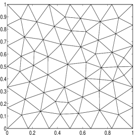
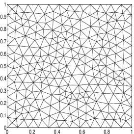
Here we give the numerical results of the multigrid scheme for the Laplace eigenvalue problem on the two dimensional domain $\Omega=(0,1)\times(0,1)$. The sequence of finite element spaces is constructed by using linear element on the series of meshes which are produced by regular refinement with $\beta=2$ (producing $\beta^{d}$ congruent subelements). In this example, we use two meshes which are generated by Delaunay method as the initial mesh $\mathcal{T}_{h_{1}}$ to produce two sequences of finite element spaces for investigating the convergence behaviors. Figure 1 shows the corresponding initial meshes: one is coarse and the other is fine.

Algorithm 4.1 is applied to solve the eigenvalue problem. For comparison, we also solve the eigenvalue problem by the direct method.

Figure 1: The coarse and fine initial meshes for Example 1.

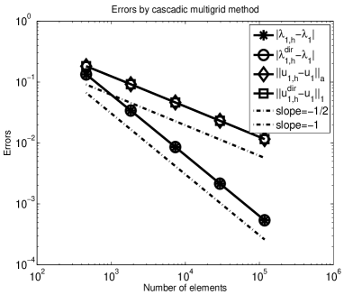
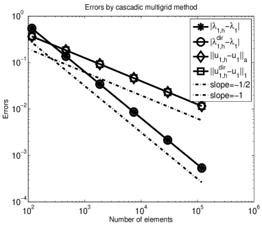
Figure 2 gives the corresponding numerical results for the first eigenvalue $\lambda_{1}=2\pi^{2}$ and the corresponding eigenfunction on the two initial meshes illustrated in Figure 1.

Figure 2: The errors of the multigrid algorithm for the first eigenvalue $2\pi^{2}$ and the corresponding eigenfunction, where $u_{h}^{\rm dir}$ and $\lambda_{h}^{\rm dir}$ denote the eigenfunction and eigenvalue approximation by direct eigenvalue solving (The left subfigure is for the coarse initial mesh in the left of Figure 1 and the right one for the fine initial mesh in the right of Figure 1).

From Figure 2, we find the multigrid scheme can obtain the optimal error estimates as same as the direct eigenvalue solving method for the eigenvalue and the corresponding eigenfunction approximations.

In order to show the efficiency of the proposed method in this paper, we also compare the running time of Algorithm 4.1 and the direct eigenvalue solving. Here we choose the package ARPACK [10, 11] as the direct eigenvalue solving tool to do the comparison. Here the conjugate gradient (CG) iteration and algebraic multigrid preconditioner are adopted to act as the linear solver in the ARPACK. In Algorithm 4.1, we only choose the CG iteration as the linear solver. Both methods are running in the same machine PowerEdge R720 with the Linux system. The corresponding results are shown in Table 1 which implies that Algorithm 4.1 can improve the efficiency of eigenvalue problem solving.

Table 1: The CPU time comparison between Algorithm 4.1 and direct eigenvalue solver. Here the number of elements in $V_{h_{1}}$ is $3968$.

Number of levels	Number of elements	time for ARpack	time for Algorithm 4.1
4	253952	7.69	2.30
5	1015808	35.96	7.98
6	4063232	191.47	31.64
7	16252928	1258.35	127.08

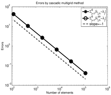
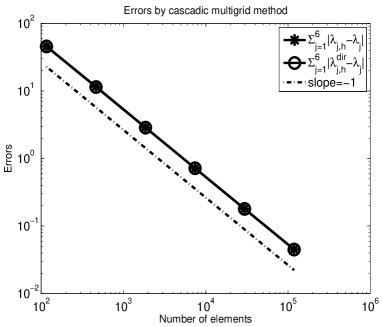
We also check the convergence behavior of multi eigenvalue approximations with Algorithm 4.1. Here the first six eigenvalues $\lambda=2\pi^{2},5\pi^{2},5\pi^{2},8\pi^{2},$ $10\pi^{2},10\pi^{2}$ are investigated. We adopt the meshes in Figure 1 as the initial meshes and the corresponding numerical results are shown in Figure 3 which also exhibits the optimal convergence rate of the multigrid scheme.

Figure 3: The errors of the multigrid algorithm for the first six eigenvalues on the unit square (The left subfigure is for the coarse initial mesh in the left of Figure 1 and the right one for the fine initial mesh in the right of Figure 1).

6.2 More general eigenvalue problem

Here we give the numerical results of the multigrid scheme for solving a more general eigenvalue problem on the unit square domain $\Omega=(0,1)\times(0,1)$:

Find $(\lambda,u)$ such that

$$\left\{\begin{array}[]{rcl}-\nabla\cdot\mathcal{A}\nabla u+\phi u&=&\lambda\rho u,\quad{\rm in}\ \Omega,\\ u&=&0,\quad\ \ \ \ {\rm on}\ \partial\Omega,\\ \int_{\Omega}\rho u^{2}d\Omega&=&1,\end{array}\right.$$ (6.1)

where

$$\mathcal{A}=\left(\begin{array}[]{cc}$$1+(x_{1}-\frac{1}{2})^{2}$$&$$(x_{1}-\frac{1}{2})(x_{2}-\frac{1}{2})$$\\ $$(x_{1}-\frac{1}{2})(x_{2}-\frac{1}{2})$$&$$1+(x_{2}-\frac{1}{2})^{2}$$\end{array}\right),$$

$\phi={\rm e}^{(x_{1}-\frac{1}{2})(x_{2}-\frac{1}{2})}$ and $\rho=1+(x_{1}-\frac{1}{2})(x_{2}-\frac{1}{2})$.

We first solve the eigenvalue problem (6.1) in the linear finite element space on the coarse mesh $\mathcal{T}_{h_{1}}$. Then refine the mesh by the regular way to produce a series of meshes $\mathcal{T}_{h_{k}}\ (k=2,\cdots,n)$ with $\beta=2$ (connecting the midpoints of each edge) and solve the auxiliary boundary value problem (3.3) in the finer linear finite element space $V_{h_{k}}$ defined on $\mathcal{T}_{h_{k}}$.

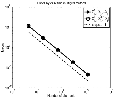
In this example, we also use two coarse meshes which are shown in Figure 1 as the initial meshes to investigate the convergence behaviors. Since the exact solution is not known, we choose an adequately accurate eigenvalue approximations with the extrapolation method (see, e.g., [12]) as the exact eigenvalue. Figure 4 gives the corresponding numerical results for the first six eigenvalue approximations and their corresponding eigenfunction approximations. Here we also compare the numerical results with the direct algorithm. Figure 4 also exhibits the optimal convergence rate of Algorithm 4.1.

Figure 4: The errors of the multigrid algorithm for the first six eigenvalues and the first eigenfunction, where $u_{h}^{\rm dir}$ and $\lambda_{h}^{\rm dir}$ denote the eigenfunction and eigenvalue approximation by direct eigenvalue solving (The left subfigure is for the coarse initial mesh in the left of Figure 1 and the right one for the fine initial mesh in the right of Figure 1).

7 Concluding remarks

In this paper, we give a type of multigrid scheme to solve eigenvalue problems. The idea here is to combine the shifted-inverse power iteration method with multilevel meshes to transform the solution of eigenvalue problem to a series of solutions of the corresponding boundary value problems which can be done by the multigrid method. As stated in the numerical examples, Eigenvalue Multigrid Scheme defined in Algorithm 4.1 for one eigenvalue can be extended to the corresponding version for multi eigenvalues (include simple and multiple eigenvalues). We state the following version of Eigenvalue Multigrid Scheme for $m$ eigenvalues.

Similarly, we first give a type of One Correction Step for Multi Eigenvalues for the given eigenpairs approximations $\{\lambda_{j,h_{k}},u_{j,h_{k}}\}_{j=1}^{m}$.

Algorithm 7.1.

One Correction Step for Multi Eigenvalues

1. Do $j=1,\cdots,m$

   • Find $\widetilde{u}_{j,h_{k+1}}\in V_{h_{k+1}}$, such that $\forall v_{h_{k+1}}\in V_{h_{k+1}}$

     $$a(\widetilde{u}_{j,h_{k+1}},v_{h_{k+1}})-\alpha_{j,k+1}b(\widetilde{u}_{j,h_{k+1}},v_{h_{k+1}})=b(u_{j,h_{k}},v_{h_{k+1}}).$$ (7.1)

   • Do the following orthogonalization and normalization

     $$\widehat{u}_{j,h_{k+1}} := \widetilde{u}_{j,h_{k+1}}-\sum_{\ell=1}^{j-1}a(\widetilde{u}_{j,h_{k+1}},u_{\ell,h_{k+1}})u_{\ell,h_{k+1}},$$ (7.2)

     $$u_{j,h_{k+1}} := \frac{\widehat{u}_{j,h_{k+1}}}{\|\widehat{u}_{j,h_{k+1}}\|_{a}}.$$ (7.3)

   End Do

2. Compute the new eigenvalue approximations

   $$\lambda_{j,h_{k+1}}=\frac{a(u_{j,h_{k+1}},u_{j,h_{k+1}})}{b(u_{j,h_{k+1}},u_{j,h_{k+1}})},\ \ \ {\rm for}\ j=1,\ldots,m.$$ (7.4)

We summarize the above two steps into

$$\{\lambda_{j,h_{k+1}},u_{j,h_{k+1}}\}_{j=1}^{m}={\it Correction}(\{\alpha_{j,k+1}\}_{j=1}^{m},\{\lambda_{j,h_{k}},u_{j,h_{k}}\}_{j=1}^{m},V_{h_{k+1}}).$$

Similarly to (3.2), we can also define a modified one correction step for multi eigenvalues where we need to solve a small dimensional eigenvalue problem.

Algorithm 7.2.

One Correction Step for Multi Eigenvalues

1. Do $j=1,\cdots,m$

   • Find $\widetilde{u}_{j,h_{k+1}}\in V_{h_{k+1}}$, such that $\forall v_{h_{k+1}}\in V_{h_{k+1}}$ satisfying

     $$a(\widetilde{u}_{j,h_{k+1}},v_{h_{k+1}})-\alpha_{j,k+1}b(\widetilde{u}_{j,h_{k+1}},v_{h_{k+1}})=b(u_{j,h_{k}},v_{h_{k+1}}).$$ (7.5)

   End Do

2. Build a finite dimensional space $\widetilde{V}_{h_{k+1}}={\rm span}\{\widetilde{u}_{1,h_{k+1}},\cdots,\widetilde{u}_{m,h_{k+1}}\}$ and solve the following eigenvalue problem:

   Find $(\lambda_{j,h_{k+1}},u_{j,h_{k+1}})\in\mathcal{R}\times\widetilde{V}_{h_{k+1}}$, $j=1,2,\cdots,m$, such that $a(u_{j,h_{k+1}},u_{j,h_{k+1}})=1$ and

   $$a(u_{j,h_{k+1}},v_{h_{k+1}}) = \lambda_{j,h_{k+1}}b(u_{j,h_{k+1}},v_{h_{k+1}}),\ \ \ \ \forall v_{h_{k+1}}\in\widetilde{V}_{h_{k+1}}.$$ (7.6)

We summarize the above two steps into

$$\{\lambda_{j,h_{k+1}},u_{j,h_{k+1}}\}_{j=1}^{m}={\it Correction}(\{\alpha_{j,k+1}\}_{j=1}^{m},\{\lambda_{j,h_{k}},u_{j,h_{k}}\}_{j=1}^{m},V_{h_{k+1}}).$$

Based on Algorithm 7.1 or 7.2, we can give the corresponding multigrid method.

Algorithm 7.3.

Eigenvalue Multigrid Scheme for Multi Eigenvalues

1. Construct a series of nested finite element spaces $V_{h_{1}},V_{h_{2}},\cdots,V_{h_{n}}$ such that (4.1) and (4.2) hold.

2. Solve the following eigenvalue problem:

   Find $(\lambda_{h_{1}},u_{h_{1}})\in\mathcal{R}\times V_{h_{1}}$ such that $a(u_{h_{1}},u_{h_{1}})=1$ and

   $$a(u_{h_{1}},v_{h_{1}}) = \lambda_{h_{1}}b(u_{h_{1}},v_{h_{1}}),\ \ \ \ \forall v_{h_{1}}\in V_{h_{1}}.$$ (7.7)

   Choose $m$ eigenpairs $\{\lambda_{j,h_{1}},u_{j,h_{1}}\}_{j=1}^{m}$ which approximate our desired eigenvalues and their eigenspaces.

3. Do $k=1,\cdots,n-1$

   Obtain new eigenpair approximations $\{\lambda_{j,h_{k+1}},u_{j,h_{k+1}}\}_{j=1}^{m}\in\mathcal{R}\times V_{h_{k+1}}$ by a correction step

   $$\{\lambda_{j,h_{k+1}},u_{j,h_{k+1}}\}_{j=1}^{m}={\it Correction}(\{\alpha_{j,k+1}\}_{j=1}^{m},\{\lambda_{j,h_{k}},u_{j,h_{k}}\}_{j=1}^{m},V_{h_{k+1}}).$$

   End Do

Finally, we obtain $m$ eigenpair approximations $\{\lambda_{j,h_{n}},u_{j,h_{n}}\}_{j=1}^{m}\in\mathcal{R}\times V_{h_{n}}$.

We can also define

$$\alpha_{j,k+1}=\max\left\{0,\frac{2(1+C_{4}/C_{5})\beta\lambda_{j,h_{k}}-\lambda_{j+1,h_{k}}}{2(1+C_{4}/C_{5})\beta-1}\right\},\ \ \ j=1,\ldots,m-1$$ (7.8)

and

$$\alpha_{m,k+1}=\max\left\{0,\frac{2(1+C_{4}/C_{5})\beta\lambda_{m,h_{k}}-\lambda_{m+1,h_{1}}}{2(1+C_{4}/C_{5})\beta-1}\right\}.$$ (7.9)

Based on the above definitions of $\alpha_{j,k+1}$, we can also give the error analysis for this version of eigenvalue multigrid method in the similar way used in Sections 3 and 4. If we use the mulgirid method (the multigrid method for indefinite problems from [15, 20]) to solve the boundary value problems included in Algorithm 7.3, the computational work involved in the multi eigenvalues version is $\mathcal{O}(m^{2}N_{n})$. Furthermore, the parallel computation can be used to solve (7.5) for different $j$. The analysis of the scheme for multi eigenvalues will be given in our future work.

We can replace the multigrid method by other types of efficient iteration schemes such as algebraic multigrid method, the type of preconditioned schemes based on the subspace decomposition and subspace corrections (see, e.g., [4, 19]), and the domain decomposition method (see, e.g., [16]). Furthermore, the framework here can also be coupled with the parallel method and the adaptive refinement technique. The ideas should be extended to other types of linear eigenvalue problems. These will be investigated in our future work.

References

• [1] I. Babuška and J. Osborn, Finite element-Galerkin approximation of the eigenvalues and eigenvectors of selfadjoint problems, Math. Comp. 52 (1989), 275–297.
• [2] I. Babuška and J. Osborn, Eigenvalue Problems, In Handbook of Numerical Analysis, Vol. II, (Eds. P. G. Lions and P. G. Ciarlet), Finite Element Methods (Part 1), North-Holland, Amsterdam, 641–787, 1991.
• [3] A. Brandt, S. McCormick and J. Ruge, Multigrid methods for differential eigenproblems, SIAM J. Sci. Stat. Comput., 4(2) (1983), 244–260.
• [4] S. Brenner and L. Scott, The Mathematical Theory of Finite Element Methods, New York: Springer-Verlag, 1994.
• [5] F. Chatelin, Spectral Approximation of Linear Operators, Academic Press Inc, New York, 1983.
• [6] P. G. Ciarlet, The finite Element Method for Elliptic Problem, North-Holland Amsterdam, 1978.
• [7] W. Hackbusch, On the computation of approximate eigenvalues and eigenfunctions of elliptic operators by means of a multi-grid method, Siam J. Numer. Anal., 16(2) (1979), 201–215.
• [8] W. Hackbusch, Multi-grid Methods and Applications, Springer-Verlag, Berlin, 1985.
• [9] X. Hu and X. Cheng, Acceleration of a two-grid method for eigenvalue problems, Math. Comp., 80(275) (2011), 1287–1301.
• [10] R. Lehoucq, K. Maschhoff, D. Sorensen and C. Yang, ARPACK Software Package, http://www.caam.rice.edu/software/ARPACK/, 1996.
• [11] R. Lehoucq, D. C. Sorensen, and C. Yang, ARPACK Users’ Guide, SIAM, Philadelphia, 1998.
• [12] Q. Lin and J. Lin, Finite Element Methods: Accuracy and Inprovement, China Sci. Tech. Press, 2005.
• [13] Q. Lin and H. Xie, A multi-level correction scheme for eigenvalue problems, Math. Comp., doi: S 0025-5718(2014)02825-1, March 10, 2014.
• [14] Q. Lin and N. Yan, The Construction and Analysis of High Efficiency Finite Element Methods, Hebei University Publishers, 1995. (in Chinese)
• [15] V. Shaidurov, Multigrid methods for finite element, Kluwer Academic Publ., Netherlands, 1995.
• [16] A. Toselli and O. Widlund, Domain Decomposition Methods: Algorithm and Theory, Springer-Verlag, Berlin Heidelberg, 2005.
• [17] H. Xie, A type of multilevel method for the Steklov eigenvalue problem, IMA J. Numer. Anal., 34(2) (2014), 592–608.
• [18] H. Xie, A multigrid method for eigenvalue problem, J. Comput. Phys., 274 (2014), 550–561.
• [19] J. Xu, Iterative methods by space decomposition and subspace correction, SIAM Review, 34(4) (1992), 581–613.
• [20] J. Xu, A new class of iterative methods for nonselfadjoint or indefinite problems, SIAM J. Numer. Anal., 29 (1992), 303–319.
• [21] J. Xu and A. Zhou, A two-grid discretization scheme for eigenvalue problems, Math. Comput., 70 (233) (2001), 17–25.
• [22] Y. Yang and H. Bi, Two-grid finite element discretization schemes based on shifted-inverse power method for elliptic eigenvalue problems, SIAM J. Numer. Anal., 49(4) (2011), 1602–1624.