Slowly varying control parameters, delayed bifurcations,
and the stability of spikes in reaction-diffusion systems

Abstract

We present three examples of delayed bifurcations for spike solutions of reaction-diffusion systems. The delay effect results as the system passes slowly from a stable to an unstable regime, and was previously analysed in the context of ODE’s in [P.Mandel and T.Erneux, J.Stat.Phys 48(5-6) pp.1059-1070, 1987]. It was found that the instability would not be fully realized until the system had entered well into the unstable regime. The bifurcation is said to have been “delayed” relative to the threshold value computed directly from a linear stability analysis. In contrast to the study of Mandel and Erneux, we analyze the delay effect in systems of partial differential equations (PDE’s). In particular, for spike solutions of singularly perturbed generalized Gierer-Meinhardt and Gray-Scott models, we analyze three examples of delay resulting from slow passage into regimes of oscillatory and competition instability. In the first example, for the Gierer-Meinhardt model on the infinite real line, we analyze the delay resulting from slowly tuning a control parameter through a Hopf bifurcation. In the second example, we consider a Hopf bifurcation of the Gierer-Meinhardt model on a finite one-dimensional domain. In this scenario, as opposed to the extrinsic tuning of a system parameter through a bifurcation value, we analyze the delay of a bifurcation triggered by slow intrinsic dynamics of the PDE system. In the third example, we consider competition instabilities triggered by the extrinsic tuning of a feed rate parameter. In all three cases, we find that the system must pass well into the unstable regime before the onset of instability is fully observed, indicating delay. We also find that delay has an important effect on the eventual dynamics of the system in the unstable regime. We give analytic predictions for the magnitude of the delays as obtained through the analysis of certain explicitly solvable nonlocal eigenvalue problems (NLEP’s). The theory is confirmed by numerical solutions of the full PDE systems.

Key words: delayed bifurcations, explicitly solvable nonlocal eigenvalue problem, Hopf bifurcation, competition instability, spike solutions, WKB, singular perturbations, reaction-diffusion systems

1   Introduction

The stability and bifurcation analysis of differential equations is one of the cornerstones of applied mathematics. In many applications, the bifurcation parameter is slowly changing, either extrinsically (e.g. parameter is experimentally controlled) or intrinsically (e.g. the bifurcation parameter is actually a slowly-changing variable). In these situations, the system can exhibit a significant delay in bifurcation: the instability is observed only as the parameter is increased well past the threshold predicted by the linear bifurcation theory, if at all. Often referred to as the slow passage through a bifurcation, and first analyzed in [1, 2], there is a growing literature on this subject (see [3] for a recent overview of the subject and references therein). Some applications of delayed bifurcations include problems in laser dynamics [2], delayed chemical reactions [4], bursting oscillations in neurons [5], and noise-induced delay of the pupil light reflex [6], and early-warning signals [7].

Delayed bifurcation phenomena is relatively well understood in the context of ODE’s. However much less is known in the context of PDE’s. The main goal of this paper is to study in detail three representative examples of delayed bifurcations in PDE’s, where explicit asymptotic results are obtainable.

In order to present our examples both analytically and numerically, we focus on slight variants of the Gierer-Meinhardt (GM) and the Gray-Scott (GS) reaction-diffusion (RD) models. However, the phenomena that we present in this paper is expected to be representative of a larger class of RD systems. The specific systems that we consider are

$$\mbox{GM\ model:\ }\qquad v_{t}=\varepsilon^{2}v_{xx}-v+\frac{v^{p}}{u^{q}}\,,\quad\tau u_{t}=Du_{xx}-u+\frac{1}{\varepsilon}\frac{v^{r}}{u^{s}}$$ (1.1)

and

$$\mbox{GS\ model:\ }\qquad v_{t}=\varepsilon^{2}v_{xx}-v+Au^{q}v^{p}\,,\quad\tau u_{t}=Du_{xx}+1-u+\frac{1}{\varepsilon}u^{s}v^{r}\,,$$ (1.2)

for certain choices of the exponents $p$, $q$, $r$, and $s$ (see below). In the singular limit $\varepsilon\rightarrow 0,$ both of these models have equilibria that consist of spike solutions, characterized by an ${\mathcal{O}}(\varepsilon)$ width localization of $v$ as $\varepsilon^{2}$ becomes asymptotically small. The component $u$ varies over a comparatively long spatial scale and is independent of $\varepsilon$. In all three of our examples, we consider spike solutions that are qualitatively similar to that shown in Figure 1(a).

To illustrate the main complications when generalizing delayed bifurcations to PDE’s, let us first review the following prototypical ODE example [2]: $\frac{du}{dt}=\left(-1+\varepsilon t\right)u,\ \ \ \ \ u(0)=u_{0}$ where $\varepsilon>0$ is a small parameter. Here, the equilibrium state is $u=0$ and can be thought of having an “eigenvalue” $\lambda(\varepsilon t)=-1+\varepsilon t$ which grows slowly in time, and becomes positive as $t$ is increased past $t=1/\varepsilon$, at which point the steady state becomes “unstable”. On the other hand, the exact solution is given by $u(t)=u_{0}\exp\left\{\frac{\left(\varepsilon t-1\right)^{2}-1}{2\varepsilon}\right\},$ which starts to grow rapidly only when the term inside the curly brackets becomes positive, that is at $t=2/\varepsilon$, well after the bifurcation threshold of $t=1/\varepsilon.$ The difference between $2/\varepsilon$ and $1/\varepsilon$ is precisely the delay in bifurcation, and is inversely proportional to the growth rate $\varepsilon$. More generally, suppose that $u_{e}$ is an equilibrium state of a system of ODE’s that changes slowly in time, so that the standard linearization $u=u_{e}+e^{\lambda t}\eta$ yields an eigenvalue $\lambda=\lambda(\varepsilon t)$ whose real part is slowly growing at a rate $\mathcal{O}(\varepsilon)$ and eventually crosses zero. One then replaces the linearization by a WKB-type anzatz $u=u_{e}+e^{\frac{1}{\varepsilon}\psi(\varepsilon t)}\eta$ which yields $\psi^{\prime}(\varepsilon t)=\lambda(\varepsilon t)$ with $\psi(0)=0.$ The condition $\psi=0$ with $t>0$ then yields an algebraic expression for the delay.

There are several novel features present in RD systems when compared to ODE systems. First, the steady state we consider is not constant, but rather a spike solution such as that shown in Figure 1(a). The stability theory for spike solutions is by now well-developed; see for example [8, 9, 10, 11, 12, 13] and a recent book [14]. One of the key ingredients is the analysis of the so-called nonlocal eigenvalue problem (NLEP), first studied in [8].

Second, although the instability thresholds $\lambda=0$ are analytically computable, the location of the unstable eigenvalue $\lambda$ itself is usually not known explicitly. However, recently, a sub-family of RD systems has been identified in [15] for which a simple asymptotic determination of this eigenvalue is possible; this is the case when $p=2r-3,$ $r>2$ in (1.1) or (1.2). For this class of RD systems, we show that an analytic prediction for the delay can be obtained in ways similar to [1, 2].

Third, the bifurcation (and its delay) can be triggered intrinsically by the motion of a spike in the system. That is, a bifurcation may be triggered not by the extrinsic tuning of a control parameter, but by dynamics intrinsic to the PDE system.

We now summarize our main results. In §2 we study the slow passage through a Hopf bifurcation. It was previously shown for both the GM model ([16, 17]) and GS models ([11, 12, 13]) that a Hopf bifurcation occurs as the parameter $\tau$ is increased past some threshold $\tau_{H}>0$. As $\tau$ is slowly tuned starting from a stable regime past the Hopf bifurcation threshold $\tau_{H}$ into an unstable regime, the amplitude of the spike in Figure 1(a) begins to oscillate periodically in time while maintaining its shape. The temporal oscillations of the amplitude are shown in Figure 1(b). However due to the slow change of parameter, there is a significant delay until the oscillations are fully realized. In §2 we compute the delay associated with this bifurcation. This is illustrated in Figure 2(a).

             

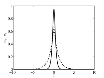
(a) $u_{e}(x)$ and $v_{e}(x)$

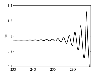
(b) amplitude oscillations in time

Figure 1: (a) The asymptotic equilibrium solution of $v$ (solid) and $u$ (dashed) for (2.1) with $\varepsilon=0.3$. The width of the spike in $v_{e}$ is proportional to $\varepsilon$, while $u_{e}$ is independent of $\varepsilon$. Both $v_{e}$ and $u_{e}$ are independent of $\tau$. (b) Typical example of amplitude oscillations in time when $\tau>\tau_{H}\approx 2.114$. The quantity plotted on the vertical axis is the height $v_{m}$ of the spike in the left figure.

             

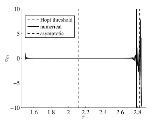
(a) $v_{m}$ versus $\tau$

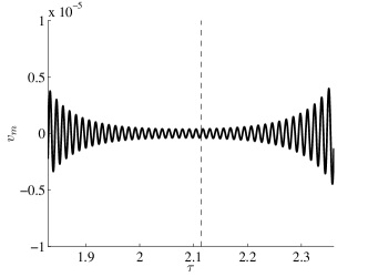
(b) numerical versus asymptotic delay

Figure 2: Delay in the Hopf bifurcation of (2.1). (a) Plot of $v_{m}(\tau)$ as defined in (2.18). The parameters are $\varepsilon=0.005$ and $\tau=1.5+\varepsilon t$. The vertical dashed line indicates the Hopf bifurcation value $\tau_{H}\approx 2.114$. The amplitude first reaches a value of one at $\tau^{*}_{m}\approx 2.75$ (thick solid line). The asymptotic prediction for $\tau^{*}$ is $\tau^{*}\approx 2.828$ (thick dashed line). (b) Magnification of (a) on a small interval of $\tau$ surrounding $\tau_{H}$. The oscillations, having decayed when $\tau<\tau_{H}$, begin growing as $\tau$ passes $\tau_{H}$. Note the scale of the $y$-axis in the right figure as compared to that of the left.

In §3, we consider a quasi-equilibrium one-spike solution of a GM model centered at $x=x_{0}$ on the domain $|x|<1$. For a spike not centered at $x=0$, the finite domain induces a slow drift of the spike toward the origin. Because the drift occurs on an asymptotically slow time scale while the characteristic time scale of a Hopf bifurcation is $\mathcal{O}(1)$, stability analysis may proceed assuming that the spike remains “frozen” at $x_{0}$. As before, a Hopf bifurcation threshold $\tau_{H}$ may be derived, but one that is dependent on the spike location $x_{0}$. That is, $\tau_{H}=\tau_{H}(x_{0};D)$, where $D$ is the inhibitor diffusivity. We show two typical curves in Figure 3 for $D=4$ (left) and $D=1$ (right). The solution is stable (unstable) below (above) the $\tau_{H}(x_{0})$ curve, while the arrows indicate the direction of spike drift. As such, a Hopf bifurcation may be triggered by dynamics intrinsic to the system and not by an extrinsic tuning of a control parameter.

             

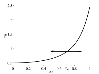
(a) $\tau_{H}(x_{0})$ for $D=4$

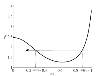
(b) $\tau_{H}(x_{0})$ for $D=1$

Figure 3: In both figures, the curve represents the Hopf bifurcation threshold $\tau=\tau_{H}$ plotted against the spike location $x_{0}$ for the GM model. The region below (above) the curve is stable (unstable). For a given value of $\tau$, the arrows indicate the direction of drift of the spike. Here, $(p,q,r,s)=(3,3,3,0)$. In the left figure, with $D=4$, $\tau_{H}(x_{0})$ is monotonic, and once the spike enters the unstable zone $x_{0}<x_{H}$, it remains in the unstable zone for all time. In the right figure, with $D=1$, $\tau_{H}(x_{0})$ is non-monotonic. For sufficiently small $\tau$, the spike may pass one threshold $x_{Hsu}$ from an stable to unstable zone, then pass through another threshold $x_{Hus}$ from an unstable to stable zone. It then remains in a stable zone for all later times.

For a given value of $\tau$, the scenario in Figure 3(a) indicates only one threshold crossing as the spike drifts toward equilibrium. However, the scenario depicted in Figure 3(b) shows the possibility of two threshold crossings for sufficiently small $\tau$. In particular, we find that, by selecting initial conditions to introduce sufficient delay into the system, the spike may pass “safely” through the unstable zone without the Hopf bifurcation ever fully setting in. In doing so, we show that delay has an important role in determining the dynamics of a system.

In §4 we consider a competition instability of a two-spike equilibrium of a singularly perturbed generalized GS model. Instead of interior spikes as in the previous examples, two half-spikes are centered at the boundaries $x=\pm 1$. A typical solution is shown in Figure 4(a). The solid line depicts two half-spikes in the activator centered at the two boundaries. Note that the inhibitor component (dashed) has been scaled by a factor of six to facilitate plotting. The spike locations remain fixed at the boundaries for all time. In addition to time-oscillatory Hopf instabilities, a solution containing two or more spikes may undergo a time-monotonic competition instability leading to the collapse of one or more spikes. In this example we study the delay in competition instability as a feed-rate parameter $A$ is decreased through the stability threshold $A_{-}$. In Figure 4(b), we show a typical result of such an instability, as the amplitude of the left spike (light solid) collapses to zero while that of the right (heavy solid) grows.

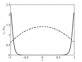
(a) two boundary spike solution

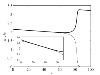
(b) spike amplitudes versus time

Figure 4: In the left figure, we show a two boundary spike equilibrium solution for $v(x)$ (solid) and $u(x)$ (dashed) in (4.1). The two spikes are of equal height. The $u$ component has been scaled by a factor of $6$ to facilitate plotting. Here, $\varepsilon=0.05$, $D=3$ and $A=4.1611$. In the right figure, we show the amplitudes of the left (light solid) and right (heavy solid) spikes as $A$ is slowly decreased past the competition threshold. The inset shows that the initial perturbation decreases the amplitude of the left spike relative to equilibrium, and increases that of the right. With $A$ starting in the stable regime, the amplitudes initially grow closer together. As $A$ passes the stability threshold, the spikes grow farther apart until the left spike amplitude collapses to 0. The results in the right figure are for $\varepsilon=0.004$ and $D=3$.

A feature of spike solutions in the Gray-Scott model is that there exists a saddle node in the feed-rate parameter $A$, which we denote by $A_{m}.$ That is, for $A<A_{m}<A_{-}$, the solution being considered ceases to exist. We give a typical bifurcation diagram in Figure 5 displaying such a saddle node. The horizontal axis is the bifurcation parameter $A$, while the vertical axis is the amplitude of the activator boundary spikes. We consider in this example only the upper solution branch, since the lower branch is known to be unstable for all $A$. The arrow shows the direction of decrease in $A$ from a stable regime (heavy solid) to the regime unstable to the competition mode (light solid). Note that the competition threshold occurs before the saddle as $A$ decreases. However, as Figure 5 suggests, with sufficient delay, the system may reach the saddle point without the competition instability fully setting in. We find in this scenario that, while the effect of the saddle is much weaker in comparison to that of the competition instability, sufficient delay in the onset of the instability may allow the saddle effect to dominate. As in the previous example, we thus find that delay may be critical in determining the eventual fate the system.

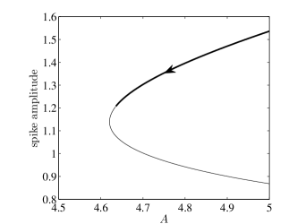
Figure 5: Bifurcation diagram for the two boundary spike solution of the GS model when $D=0.4$. On the upper branch, the solid segment indicates stable solutions, while the light solid segment indicates solutions unstable to the competition mode. The stability transition occurs at $A=A_{-}\approx 4.6351$, while the saddle node occurs at $A=A_{m}\approx 4.6206$. The arrow indicates the evolution of the spike amplitude as $A$ is decreased. The lower branch is unstable for all values of $A$.

In each of the following examples, we focus on three main objectives. We first seek to demonstrate analytically why a delay in the onset of an instability occurs when a system is slowly tuned past a stability threshold. We then show that an explicitly solvable nonlocal eigenvalue problem (NLEP) allows for an analytic prediction of the magnitude of delay. Finally, we compare analytic predictions of delay to numerical results obtained from solving the full PDE systems. The construction of the spike equilibrium and quasi-equilibrium solutions, as well as the subsequent stability analysis leading to an explicitly solvable NLEP, follow from similar past problems. Since our emphasis is on illustrating the delay effect, we include only enough of the analysis to meet our stated objectives, and relegate the remaining to the appendix.

2   Example 1: Hopf bifurcation of a one-spike solution on the infinite line

In the first example, we consider a Hopf bifurcation of a one-spike equilibrium solution to a particular exponent set of the GM system (1.1) on the infinite real line

$$v_{t}=\varepsilon^{2}v_{xx}-v+\frac{v^{3}}{u^{2}}\,,\qquad-\infty<x<\infty\,,\qquad t>0\,,\qquad v\to 0\quad\mbox{as}\quad|x|\to\infty\,,$$ (2.1a)

$$\tau u_{t}=u_{xx}-u+\frac{v^{3}}{\varepsilon}\,,\qquad-\infty<x<\infty\,,\qquad t>0\,,\qquad u\rightarrow 0\quad\mbox{as}\quad|x|\rightarrow\infty\,.$$ (2.1b)

The primary motivation for this choice of exponents is that they satisfy the key relationship $p=2r-3$ from [15]. This relationship allows for an explicit computation of the large eigenvalue of the NLEP problem associated with the linearization around the spike equilibrium. Here, $\varepsilon^{2}\ll 1$ is the diffusivity of the activator component $v$, while the diffusivity of the inhibitor component $u$ is set to unity without loss of generality. We consider an equilibrium solution of (2.1) for which the activator takes the form of a single spike of width $\mathcal{O}(\varepsilon)$ centered at $x=0$ while the inhibitor varies over an ${\mathcal{O}}(1)$ spatial scale. The parameter $\tau$ is taken to be the bifurcation parameter. When $\tau$ is large, the inhibitor responds sluggishly to small activator deviations from equilibrium, leading to oscillations in the height of the activator spike. When $\tau$ is below a certain threshold value $\tau_{H}$, the response is fast enough such that oscillations decay in time. When $\tau$ exceeds $\tau_{H}$, a Hopf bifurcation occurs and oscillations grow in time. In this section, we analyze the scenario where $\tau$ is slowly increased past $\tau_{H}$ starting from $\tau=\tau_{0}<\tau_{H}$.

2.1   Analytic calculation of delay

From [15], the one-spike equilibrium solution of (2.1) takes the form

$$v_{e}\sim U_{0}w\left(\varepsilon^{-1}x\right)\,,\qquad u_{e}\sim\frac{U_{0}}{G(0,0)}G(x;0)\,,$$ (2.2)

where $w(y)$, $G(x,x_{0})$, and $U_{0}$ are defined by

$$w(y)=\sqrt{2}\operatorname{sech}y\,;\qquad\int_{-\infty}^{\infty}\!w^{3}\,dy\equiv b=\pi\sqrt{2}\,,\qquad G(x;x_{0})=\frac{1}{2}e^{-\lvert x-x_{0}\rvert}\,,\qquad U_{0}=\frac{1}{\sqrt{b\,G(0;0)}}\,.$$ (2.3)

We plot the solutions for $v$ (solid) and $u$ (dashed) in Figure 1(a) on a domain of length $20$ for $\varepsilon=0.3$. Note that the equilibrium solution (2.2) is independent of $\tau$, which only affects stability.

In Appendix A, we perform a linear stability analysis of the equilibrium solution (2.2) by perturbing the equilibrium solution as

$$v=v_{e}+e^{\lambda t}\phi\,,\qquad u=u_{e}+e^{\lambda t}\eta\,;\qquad\phi,\eta\ll 1\,,$$ (2.4)

where $\lambda$ and $(\phi,\eta)$ are the associated eigenvalue and eigenfunctions, respectively. From the resulting linearized equation, we derive a nonlocal eigenvalue problem (NLEP) governing its $\mathcal{O}(1)$ time scale stability to amplitude perturbations. Solving the NLEP explicitly, we obtain an exact expression for the eigenvalue $\lambda$ in terms of $\tau$ as

$$\lambda(\tau)=3-\frac{9}{\sqrt{1+\tau\lambda}}\,.$$ (2.5)

The function $\lambda(\tau)$ in (2.5) may be inverted for $\tau$, yielding

$$\tau(\lambda)=\frac{81}{\lambda(3-\lambda)^{2}}-\frac{1}{\lambda}\equiv f(\lambda)\,.$$ (2.6)

To analyze (2.5), we define the function

$$\mathcal{G}(\lambda)\equiv\frac{9}{3-\lambda}\,.$$ (2.7)

Then $\lambda$ is a root of the equation

$$\sqrt{1+\tau\lambda}=\mathcal{G}(\lambda)\,.$$ (2.8)

The function $\mathcal{G}(\lambda)$ is positive (negative) for $\lambda<3$ ($\lambda>3$), and approaches $\pm\infty$ as $\lambda\to 3^{\mp}$. With $\mathcal{G}(0)=3$, $\mathcal{G}^{\prime}>0$ and $\mathcal{G}^{\prime\prime}>0$ on $0<\lambda<3$, we find that (2.8) has no positive real roots if $\tau\ll 1$, and two positive real roots on $0<\lambda<3$ if $\tau\gg 1$. These two cases are illustrated schematically in Figure 6 below.

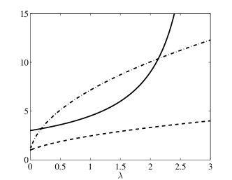
Figure 6: The function $\mathcal{G}(\lambda)$ in (2.7) is indicated by the solid curve on the interval $[0,3]$. The dashed curve depicts the function $\sqrt{1+\tau\lambda}$ for $\tau$ sufficiently small so that it does not intersect $\mathcal{G}(\lambda)$. The dash-dotted curve depicts $\sqrt{1+\tau\lambda}$ for large $\tau$. In this case, there are two intersections, representing two positive real roots of (2.8).

The argument principle can be applied to show that the two positive real roots when $\tau\gg 1$ are the only two roots for $\lambda$ in the right-half plane ([15]). Further, it can be shown that there are no roots in the right-half plane for $\tau$ sufficiently small. Since $\lambda=0$ is never a solution of (2.8) for finite $\tau$, by continuity of the roots of (2.8) in $\tau$, there exists a critical value $\tau=\tau_{H}$ for which $\lambda=i\lambda_{I}$ for some positive real $\lambda_{I}$. From (2.8) the unique Hopf bifurcation point is

$$\tau_{H}=\frac{1}{36}\left[2c^{2}+12+2c\sqrt{c^{2}+12}\right]>\frac{3}{2},\quad c\equiv\frac{3\sqrt{3}}{2};\qquad\lambda_{I}=3\sqrt{1-\frac{2}{3\tau_{H}}}\,.$$ (2.9)

We thus conclude that $\Re(\lambda)<0$ when $\tau<\tau_{H}$, and $\Re(\lambda)>0$ when $\tau>\tau_{H}$.

To understand the phenomenon of delayed Hopf bifurcation as $\tau=\tau(\sigma t)$, $\sigma\ll 1$, is slowly increased from $\tau=\tau_{0}<\tau_{H}$ into the unstable regime $\tau>\tau_{H}$, we must track the decay of the perturbation in (2.4) during the time interval that $\tau$ is below $\tau_{H}$. The longer the system remains in the stable regime, the more the perturbation decays, and therefore the more time it requires for the perturbation to grow to its original amplitude when $\tau>\tau_{H}$. To analyze this effect, we follow [2] and rewrite the perturbations in (2.4) by applying the WKB ansatz

$$v=v_{e}+e^{\frac{1}{\sigma}\psi(\xi)}\phi\,,\qquad u=u_{e}+e^{\frac{1}{\sigma}\psi(\xi)}\eta\,,\qquad\xi=\sigma t\,,\quad\sigma\ll 1;\qquad\phi,\eta\ll 1\,.$$ (2.10)

Differentiating (2.10) with respect to $t$, we calculate that

$$v_{t}=\frac{1}{\sigma}\psi^{\prime}(\xi)\frac{d\xi}{dt}e^{\frac{1}{\sigma}\psi(\xi)}\phi\,,\qquad u_{t}=\frac{1}{\sigma}\psi^{\prime}(\xi)\frac{d\xi}{dt}e^{\frac{1}{\sigma}\psi(\xi)}\eta\,.$$ (2.11)

Noting that $d\xi/dt=\sigma$ in (2.11), and upon replacing $\tau$ in (2.1) by $\tau=\tau(\xi)$ and linearizing, we find that $\psi^{\prime}(\xi)$ satisfies the same eigenvalue problem as does the stationary eigenvalue $\lambda$ in (2.5). That is, we obtain the ordinary differential equation (ODE) for $\psi(\xi)$

$$\psi^{\prime}(\xi)\equiv\psi_{R}^{\prime}(\xi)+i\psi_{I}^{\prime}(\xi)=3-\frac{9}{\sqrt{1+\tau(\xi)\psi^{\prime}(\xi)}}\,,\qquad\psi(0)=0\,.$$ (2.12)

The initial condition for $\psi$ in (2.12) is set without loss of generality by noting that any prefactors in the perturbation may be absorbed into $\phi$ and $\eta$. In the following, we assume that $\tau(\xi)$ is a monotonically increasing function of $\xi$ with $\tau(0)=\tau_{0}<\tau_{H}$.

The correspondence between $\psi^{\prime}$ with $\lambda$ implies that $\psi_{R}(\sigma t)$ is a decreasing function of time as long as $\tau$ remains below the threshold $\tau=\tau_{H}$. This is illustrated in Figure 7 below, as $\psi_{R}^{\prime}$ is negative for all $\tau<\tau_{H}\approx 2.114$, where $\tau_{H}$ is computed from (2.9). During this period, the perturbation decays to an amplitude of order $\mathcal{O}(e^{-1/\sigma})$, with $\sigma\ll 1$. The amplitude only begins to grow once $\tau$ is ramped up past $\tau_{H}$. The time $t^{*}>0$ at which the perturbation grows back to its original amplitude occurs when $\psi_{R}=0$. The longer the system remains in the stable regime, the more $\tau(\sigma t)$ must be ramped up past $\tau_{H}$ before the perturbation amplitude is restored and the instability is fully realized. We define the delay to be the amount by which $\tau(\sigma t^{*})\equiv\tau^{*}$ exceeds $\tau_{H}$, and refer to this as the delay effect.

To calculate the value of $\tau^{*}$ analytically at which $\psi_{R}=0$, we begin by using for $\tau(\xi)$ a linear ramping function

$$\tau(\xi)=\tau_{0}+\xi\,,\qquad\xi/t=\sigma\ll 1\,,\qquad\tau_{0}<\tau_{H}\,.$$ (2.13)

Integrating the relation $\psi^{\prime}(\xi)=\lambda$ with respect to slow time $\xi$, we obtain

$$\int_{0}^{\psi(\tau_{1})}\!\psi^{\prime}\,d\xi=\int_{0}^{\xi_{1}}\!\lambda\,d\xi=\int_{\tau_{0}}^{\tau_{1}}\!\lambda\,d\tau\,,$$ (2.14)

where $\tau_{1}=\tau(\xi_{1})$, and where we have used (2.13) to change the variable of integration to $\tau$. Using (2.6) to again change the variable of integration of the third integral in (2.14) from $\tau$ to $\lambda$, we calculate

$$\psi(\tau_{1})=[\lambda_{1}f(\lambda_{1})-F(\lambda_{1})]-[\lambda_{0}f(\lambda_{0})-F(\lambda_{0})]\,,$$ (2.15)

where $\lambda_{0}=\lambda(\tau_{0})$, $f(\lambda)$ is defined in (2.6), $\tau_{1}=f(\lambda_{1})$, and

$$F(\lambda)=\int^{\lambda}\!f(s)\,ds=8\log\lambda-9\log(\lambda-3)-\frac{27}{\lambda-3}\,.$$ (2.16)

Setting the right-hand side of (2.15) to 0 with $F(\lambda)$ defined in (2.16) yields an algebraic equation for $\lambda_{1}=\lambda^{*}$. We then calculate $\tau^{*}=f(\lambda^{*})$ using (2.6). Note that $\tau^{*}$ is independent of $\varepsilon$. That is, the delay in terms of $\tau$ is independent of the rate at which it is decreased. However, the duration in time of the delay increases monotonically with $1/\varepsilon$, as observed in [2].

Our analysis, confirmed by numerical computations, shows that the farther $\tau$ starts below threshold in the stable regime, the farther it must be increased above threshold for the instability to fully set in. In Figure 8, we illustrate the delay phenomenon for a range of values of $\tau_{0}$. Denoting $\tau^{\ast}$ as the value of $\tau$ at which $\psi_{R}$ changes sign from negative to positive, we find that the farther into the stable regime $\tau_{0}$ is, the farther into the unstable regime $\tau^{\ast}$ must be for oscillations resulting from the Hopf bifurcation to grow to the size of the original perturbation. The increasing relationship between the “initial buffer” $\tau_{H}-\tau_{0}$ and the distance above threshold before onset $\tau^{\ast}-\tau_{H}$ is typical in all of our findings, regardless of the triggering parameter or mechanism.

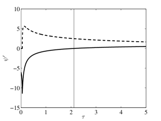
Figure 7: A plot of the real (heavy solid) and imaginary (dashed) parts of the solution to the algebraic equation for $\psi^{\prime}$ in (2.12). At $\tau=\tau_{H}\approx 2.114$ (solid vertical line), $\Re(\psi^{\prime})=0$, while $\Re(\psi^{\prime})<0$ ($\Re(\psi^{\prime})>0$) when $\tau<\tau_{H}$ ($\tau>\tau_{H}$).

2.2   Numerical validation

In this section, we compare the asymptotic results for delay obtained above with numerical results computed from the GM model (2.1). We replace $\tau$ in (2.1b) with a slowly varying function $\tau=\tau(\varepsilon t)$ according to (2.13). To solve (2.1) numerically, we used a semi-implicit second order predictor-corrector method in time and pseudo-spectral Fourier method in space. The following results did not differ significantly when the number of grid points was doubled while the time-step was decreased by a factor of four. To approximate the infinite line, we used a computational domain length of $L=20$. Doubling $L$ did not alter the results significantly.

The initial conditions were taken as a perturbation of the true equilibrium

$$v(x,0)=v_{e}^{*}(x)\left[1+\delta\cos\left(\frac{\pi x}{\varepsilon}\right)e^{-\left(\frac{x}{\varepsilon}\right)^{2}}\right]\,,\qquad u(x,0)=u_{e}^{*}(x)\,,$$ (2.17)

with $\delta$ small. The true equilibrium $(v,u)=(v_{e}^{*},u_{e}^{*})$ was computed starting from $(v_{e},u_{e})$ in (2.2) and integrating in time with fixed $\tau=\tau_{0}$ until a steady state was reached. In this way, initial transient oscillations resulting from the error of the leading order equilibrium solution in (2.2) were removed. To compare results of numerical computations to the asymptotic results of Figure 8, we define the oscillation amplitude

$$v_{m}(\tau(\varepsilon t))\equiv\frac{v(0,t)-v_{e}(0)}{v(0,0)-v_{e}(0)}\,,$$ (2.18)

where the denominator in (2.18) acts to normalize results over different values of $\delta$ so that $v_{m}(\tau_{0})=1$. We found that $v_{m}(\tau)$ behaved rather consistently over a range of values for $\delta$. According to (2.10), we define $\tau^{*}_{m}$ to be the value of $\tau>\tau_{0}$ at which the value of $|v_{m}(\tau)|$ first exceeds unity. In Figure 2(a), we plot a typical case of $v_{m}(\tau)$ with $\tau_{0}=1.5<\tau_{H}$ and $\varepsilon=0.005$. The vertical dashed line indicates the critical Hopf bifurcation value $\tau_{H}$. We found in this instance that $\tau^{*}_{m}\approx 2.75$, while the asymptotic result gives $\tau^{*}\approx 2.828$. These two values are indicated by the thick solid and thick dashed lines in Figure 2(a), respectively. Defining the percentage error as

$$\mbox{error}\equiv\frac{(\tau^{*}-\tau_{H})-(\tau^{*}_{m}-\tau_{H})}{\tau^{*}-\tau_{H}}\,,$$ (2.19)

we calculate an error of approximately $5.26\%$. Repeating the same run with double the value of $\varepsilon$ yielded an error of approximately $10.86\%$. In most cases, we found the error to approximately double as $\varepsilon$ was doubled.

It can be seen in Figure 2(a) that the oscillations only become observable well after $\tau$ has increased past the Hopf bifurcation value $\tau_{H}$. However, with sufficient enlargement as shown in Figure 2(b), we find that oscillations decay up until $\tau$ has increased to $\tau_{H}$, and then begin to grow thereafter. Since $\tau$ remains in the stable regime for an extended time, the oscillation amplitude decays to order $1\times 10^{-6}$ at its smallest value when $\tau=\tau_{H}$, thereby delaying the time it takes for it to grow back to its original value.

Repeating the above procedure for various $\tau_{0}$, we obtain the results presented in Figure 8. We observe excellent agreement between the asymptotic and numerical results over the range of $\tau_{0}$ for which we were able to obtain data. Numerical results for larger values of $\tau_{H}-\tau_{0}$ were generally difficult to obtain, especially for small values of $\varepsilon$. The reason is that the smaller $\tau_{0}$ and $\varepsilon$ are, the more time the system spends in the stable regime and so the more time over which the perturbation decays. Once the oscillation amplitude decays to below machine precision, we observe no ensuing instabilities even when $\tau$ was increased far past $\tau^{*}$. In effect, the system loses the memory of its history accounted for in the asymptotic analysis, which then would no longer apply.

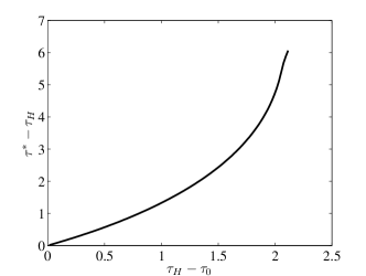
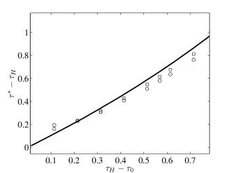
Figure 8: (a) The delay phenomenon obtained by computing the value $\tau^{*}$ at which $\Re(\psi)$ changes from negative to positive, for different values of $\tau_{0}$. The figure shows that the smaller $\tau_{0}$ is, the larger $\tau^{*}$ must be for the Hopf bifurcation to be fully realized. Here, $\tau_{H}\approx 2.114$ is the Hopf bifurcation threshold so that $\tau_{H}-\tau_{0}$ is the initial buffer while $\tau^{*}-\tau_{H}$ is the distance above threshold. (b) Numerical results of delay for $\varepsilon=0.01$ (circles) and $\varepsilon=0.005$ (squares) compared against the asymptotic results (solid curve) as in (a). The errors for $\varepsilon=0.005$, as defined in (2.19), for most values of $\tau_{0}$ are approximately half those for $\varepsilon=0.01$.

In this section, we considered a bifurcation triggered by an extrinsic tuning of the control parameter $\tau$. In contrast, the next section will consider the triggering of a Hopf bifurcation by dynamics intrinsic to the system. On a finite domain, we find the possibility of a non-monotonicity in the Hopf bifurcation threshold, a feature not present in the example just considered. By carefully setting initial conditions to induce sufficient delay, we find that this feature allows a spike to pass safely through a Hopf-unstable zone into a stable zone with no subsequent instabilities.

3   Example 2: Hopf bifurcation of a one-spike solution on a finite domain

In this section, we consider the general GM system on a finite one-dimensional domain

$$v_{t}=\varepsilon^{2}v_{xx}-v+\frac{v^{p}}{u^{q}}\,,\qquad-1<x<1\,,\qquad v_{x}(\pm 1,t)=0\,,\qquad t>0\,,$$ (3.1a)

$$\tau u_{t}=Du_{xx}-u+\frac{1}{\varepsilon}\frac{v^{r}}{u^{s}}\,,\qquad-1<x<1\,,\qquad u_{x}(\pm 1,t)=0\,,\qquad t>0\,,$$ (3.1b)

where the exponents, $p,q,r,s\geq 0,$ satisfy the relation $qr/(p-1)-s-1>0$. To obtain an explicitly solvable NLEP as in Section 2, we require the additional relation

$$p=2r-3\,,\quad r>2\,.$$ (3.2)

In the previous section, a Hopf bifurcation was triggered by an extrinsic tuning of the parameter $\tau$. In contrast, the Hopf bifurcation that we consider in this section is intrinsically triggered by slow spike dynamics. That is, an initially stable quasi-equilibrium profile centered at $x=x_{0}>0$ undergoes a slow $\mathcal{O}(\varepsilon^{2})$ drift towards its equilibrium location of $x_{0}=0$ and triggers a Hopf bifurcation before reaching equilibrium. At the Hopf bifurcation, the associated eigenvalue is of $\mathcal{O}(1)$ and imaginary. We emphasize that all parameters in (3.1) remain constant, with only the intrinsic motion of the spike able to trigger a bifurcation.

Two scenarios are possible. The first is illustrated schematically in Figure 3(a) for $(p,q,r,s)=(3,3,3,0)$ and $D=4$. The black curve represents the Hopf bifurcation threshold $\tau=\tau_{H}$ plotted against the spike location $x_{0}$. The quasi-equilibrium solution is stable (unstable) when $\tau$ is below (above) the threshold vale $\tau_{H}$. Alternatively, for a given value of $\tau$, the quasi-equilibrium solution is stable (unstable) when $x_{0}>x_{H}(\tau)$ ($x_{0}<x_{H}(\tau)$). Starting at $x_{0}(0)>x_{H}$, Figure 3(a) illustrates schematically the intrinsic triggering of a Hopf bifurcation due to the direction of drift, indicated by the arrow. As in the case of §2, oscillations are expected to decay while $x_{0}<x_{H}$, beginning to grow only when the spike enters the unstable zone. The amplitude of oscillations when $x_{0}=x_{H}$ must then be smaller than that of the original perturbation at $x_{0}=x_{0}(0)$. The delay refers to how far the spike must travel into the unstable zone before the oscillation amplitude is restored to that of the original perturbation and the Hopf bifurcation is considered to be fully realized.

For the same exponent set, Figure 3(b) shows an example of the second scenario where the function $\tau_{H}(x_{0})$ is non-monotonic when $D=1$. For a given $\tau$ sufficiently small, there exists two Hopf-stability thresholds. The first, $x_{Hsu}$, occurs as the spike drifts from a stable to unstable zone. The second, $x_{Hus}$, occurs as the spike re-enters a stable region from an unstable region. If the predicted delay is sufficiently large, the spike may pass “safely” through the unstable zone without the Hopf bifurcation ever being fully realized. Both of these scenarios are demonstrated numerically in the following section.

In Appendix B, we construct a quasi-equilibrium one-spike solution to (3.1) and derive an ODE describing the slow drift of the spike profile. Assuming that the spike location remains frozen with respect to an $\mathcal{O}(1)$ time scale, we perform a linear stability analysis to calculate the Hopf bifurcation threshold $\tau_{H}(x_{0})$, examples of which are shown in Figure 3. By similar arguments to §2.1, we obtain a coupled system for the spike location and the time-dependent eigenvalue $\psi(\varepsilon^{2}t)$, from which we compute the asymptotic prediction of delay. As before, we present only the results of this analysis, and refer the reader to Appendix B for more details.

3.1   Asymptotic prediction of delay

The one-spike quasi-equilibrium solution to (3.1), with spike centered at $x=x_{0}$, is given by

$$v_{qe}=U_{0}^{q/(p-1)}w(\varepsilon^{-1}(x-x_{0}))\,,\qquad u_{qe}=\frac{U_{0}}{G_{00}}G(x;x_{0})\,.$$ (3.3)

Here, $w(y)$ is the solution of the equation

$$w^{\prime\prime}-w+w^{p}=0\,,\qquad-\infty<y<\infty\,,\qquad w(0)>0\,,\qquad w^{\prime}(0)=0\,,\qquad w\to 0\quad\mbox{as}\quad|y|\to\infty\,,$$ (3.4)

given by [11]

$$w(y)=\left\{\frac{p+1}{2}\operatorname{sech}^{2}\left(\frac{p-1}{2}y\right)\right\}^{1/(p-1)}\,;\qquad b_{r}\equiv\int_{-\infty}^{\infty}\!w^{r}\,dy\,.$$ (3.5)

In (3.3), $G(x;x_{0})$ is given by

$$G(x;x_{0})=G_{00}\left\{\begin{array}[]{lr}\frac{\cosh\left(\theta_{0}(1+x)\right)}{\cosh\left(\theta_{0}(1+x_{0})\right)}\,,&x<x_{0}\,,\\ \frac{\cosh\left(\theta_{0}(1-x)\right)}{\cosh\left(\theta_{0}(1-x_{0})\right)}\,,&x>x_{0}\,,\end{array}\right.$$ (3.6)

while $G_{00}$ and $U_{0}$ are given by

$$G_{00}=\frac{1}{\sqrt{D}\left[\tanh\left(\theta_{0}(1+x_{0})\right)+\tanh\left(\theta_{0}(1-x_{0})\right)\right]}\,;\qquad\theta_{0}\equiv\frac{1}{\sqrt{D}}\,,$$ (3.7)

and

$$U_{0}=\frac{1}{(b_{r}G_{00})^{1/M}}\,;\qquad M\equiv\frac{qr}{p-1}-s-1\,,$$ (3.8)

respectively, where $b_{r}$ is defined in (3.5).

When $x_{0}\neq 0$, the spike profile drifts on a slow time scale according to the equation

$$\frac{dx_{0}}{d\sigma}=-\frac{q}{(p-1)\sqrt{D}}\left[\tanh\left(\theta_{0}(1+x_{0})\right)-\tanh\left(\theta_{0}(1-x_{0})\right)\right]\equiv F(x_{0})\,;\qquad\sigma\equiv\varepsilon^{2}t\,,$$ (3.9)

where $\theta_{0}$ is defined as in (3.7). Note that $F(x_{0})<0$ ($F(x_{0})>0$) when $x_{0}>0$ ($x_{0}<0$) with $F(0)=0$ so that the dynamics of the spike are always monotonic toward the equilibrium point $x=0$. The corresponding evolution of the spike amplitude can be obtained from (3.3), (3.7), and (3.8). In Figure 9, we show the spike at three different times during its evolution, beginning at $x_{0}(0)=0.7055$. As time increase, the spike drifts toward the origin while keeping a constant profile, changing only in height. The parameters are $(p,q,r,s)=(3,3,3,0)$, $D=4$, and $\tau=0.01$. By Figure 3(a), this value of $\tau$ is well below threshold for all $0<x_{0}<1$, and so no oscillations in spike amplitude are present.

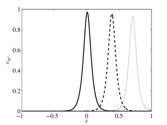
Figure 9: Plots of $v_{qe}$ at various times during its evolution according to (3.9). The spike increases in height as it drifts toward $x_{0}=0$. The parameters are $(p,q,r,s)=(3,3,3,0)$, $\varepsilon=0.05$, $D=4$, and $\tau=0.01$. By Figure 3(a), this value of $\tau$ is well below threshold for all $x_{0}$, and so no oscillations in spike amplitude are present. The times depicted are $t=0$ (dotted), $t=400$ (dashed), and $t=2800$ (solid).

To find the Hopf bifurcation threshold, we perturb the quasi-equilibrium solution (3.3) by

$$v=v_{qe}+e^{\lambda t}\phi\,,\qquad u=u_{qe}+e^{\lambda t}\eta\,;\qquad\phi,\eta\ll 1\,.$$ (3.10)

Analysis of the resulting linearized equation with $p$ satisfying (3.2) leads to an explicitly solvable NLEP, from which we obtain the equation for the eigenvalue $\lambda$

$$\lambda=\beta-\frac{r}{2}\chi(\lambda,x_{0})\,,\qquad\beta\equiv r^{2}-2r>0\,,$$ (3.11)

where $\chi(\lambda,x_{0})$ is given by

$$\chi=rq\frac{G_{\lambda 00}}{G_{00}}\frac{1}{1+sG_{\lambda 00}I_{r}}\,;\qquad I_{r}\equiv U_{0}^{Rr-s-1}\int_{-\infty}^{\infty}\!w^{r}\,dy\,,\qquad R\equiv\frac{q}{p-1}\,.$$

Here, $G_{00}$ is given by (3.7), while $G_{\lambda 00}$ is defined as

$$G_{\lambda 00}=\frac{1}{\sqrt{D(1+\tau\lambda)}\left[\tanh\left(\theta_{\lambda}(1+x_{0})\right)+\tanh\left(\theta_{\lambda}(1-x_{0})\right)\right]}\,;\qquad\theta_{\lambda}\equiv\theta_{0}\sqrt{1+\tau\lambda}\,,$$

with $\theta_{0}$ defined in (3.7). By setting $\lambda=i\lambda_{I}$, we may solve the real and imaginary parts of (3.11) for $\lambda_{I}\in\mathbb{R}$ and the Hopf bifurcation threshold $\tau_{H}$ as functions of $x_{0}$. The relation $\tau_{H}(x_{0})$ for two different values of $D$ is shown in Figure 3.

To account for the slow dynamics and the dependence of $\lambda$ on $x_{0}$, we proceed as in §2.1 and replace (3.10) with the WKB ansatz

$$v=v_{qe}+e^{\frac{1}{\varepsilon^{2}}\psi(\sigma)}\phi\,,\qquad u=u_{qe}+e^{\frac{1}{\varepsilon^{2}}\psi(\sigma)}\eta\,,\qquad\sigma\equiv\varepsilon^{2}t\,.$$ (3.12)

Substituting (3.12) into (3.1) and linearizing to identify the equivalence $\psi^{\prime}=\lambda$, we obtain for $\psi(\sigma)$

$$\psi(\sigma)=\int_{0}^{\sigma}\!\lambda\,d\sigma=\int_{x_{0}(0)}^{x_{0}(\sigma)}\lambda(x_{0})\frac{1}{F(x_{0})}\,dx_{0}\,.$$ (3.13)

In (3.13), we have taken $\psi(0)=0$ without loss of generality, and used (3.9) to change the variable of integration from $\sigma$ to $x_{0}$. The delay phenomenon may be understood in the same manner as in §2. By setting $x_{0}(0)>x_{H}$ in the Hopf-stable regime so that $\Re(\lambda)<0$, $\psi(\sigma)$ will be negative and decreasing until $x_{0}(\sigma)$ reaches $x_{H}$. During this time, the oscillations decay to an $\mathcal{O}(e^{-1/\varepsilon^{2}})$ amplitude. The spike will then enter the unstable regime, at which time $\psi(\sigma)$ will begin to increase towards $0$. Assuming the scenario depicted in Figure 3(a), $\psi(\sigma)$ will then reach 0 for some $\sigma=\sigma^{*}$ for which $x_{0}(\sigma^{*})=x_{0}^{*}<x_{H}$. We define this as the time when the Hopf bifurcation is fully realized. That is,

$$\int_{x_{0}(0)}^{x_{0}(\sigma^{*})}\lambda(x_{0})\frac{1}{F(x_{0})}\,dx_{0}=0.$$ (3.14)

Along with (3.11), (3.14) constitutes a set of algebraic equations for $x_{0}^{*}$ as a function of $x_{0}(0)$. As in §2.1, the delay in terms of $x_{0}$ is independent of $\varepsilon$. For $(p,q,r,s)=(3,3,3,0),$ we show in Figure 10 the relation between the delay $x_{H}-x_{0}^{*}$ and $x_{0}(0)-x_{H}$, the “initial buffer,” or how far into the stable zone the spike is located at $t=0$. The increasing function indicates that the larger the initial buffer, the larger the delay. Qualitatively, the more time the spike remains in the stable zone, the more its oscillation amplitude decays, and so the more time it must spend in the unstable zone for the oscillations to recover to their original amplitude.

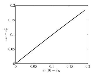
Figure 10: A plot of delay, $x_{H}-x_{0}^{*}$, versus the “initial buffer,” $x_{0}(0)-x_{H}$, where $x_{0}(0)$ is the initial location of the spike, $x_{H}$ is the Hopf bifurcation value, and $x_{0}^{*}$ is the spike location at which the oscillation amplitude recovers to the size of the original perturbation. The exponents ($(p,q,r,s)=(3,3,3,0)$) and value of $D$ ($D=4)$ correspond to the monotonic $\tau_{H}(x_{0})$ depicted in Figure 3(a), while $\tau$ is set at $0.891$.

For the scenario depicted in Figure 3(b), initial conditions may be chosen to induce sufficient delay so that $\psi$ will not increase past $0$ before it passes through the unstable zone. In this case, the spike can pass safely through the unstable zone without the Hopf bifurcation ever being fully realized. In the following section, we present numerical examples of both scenarios. Due to the sensitive nature of the numerical computations, we compare the numerical results to asymptotic results only for the case where $\tau_{H}(x_{0})$ is monotonic. Numerical results for the non-monotonic case serve only to illustrate the qualitative aspect of the theory.

3.2   Numerical validation

We illustrate the theory by numerically solving (3.1) for two exponent sets $(p,q,r,s)=(3,2,3,0)$ and $(p,q,r,s)=(3,3,3,0)$. The time integration was performed using the MATLAB pdepe() routine. The initial conditions were taken as a perturbation of a “true quasi-equilibrium” state $(v(x,0),u(x,0))$ = $(v_{eq}^{*}(x),u_{eq}^{*}(x))$, similar to that of (2.17). To obtain $(v_{eq}^{*}(x),u_{eq}^{*}(x))$, we started from initial conditions $(v_{eq},u_{eq})$, the asymptotic result given in (3.3), and integrated in time to allow for transient effects to decay. The spike location in $(v_{eq},u_{eq})$ was set so that, after the initial integration, $(v_{eq}^{*}(x),u_{eq}^{*}(x))$ had the desired spike location. All values for the initial spike locations stated below are reflected in $(v_{eq}^{*}(x),u_{eq}^{*}(x))$. We first present results for the scenario in Figure 3(a), where $\tau_{H}(x_{0})$ is monotonic.

The results below for $\varepsilon=0.007$ were obtained with $2000$ grid points, while those for $\varepsilon=0.005$ were obtained with $3000$ grid points. Unlike the static problem of Section (2), we found that this problem displayed sensitivity to the number of grid points used. In particular, we found that decreasing mesh size tended to trigger the Hopf bifurcation earlier than expected. We conjecture this may be due to rounding errors associated with a large number of grid points. Further, while the asymptotic results become more accurate as $\varepsilon$ is decreased, we found that small $\varepsilon$ caused spike oscillations to decay so much that the grid was unable to resolve the oscillations as the spike moved from one grid location to the next. To compensate for small $\varepsilon$, we set initial spike locations close to threshold so that oscillations remained of sufficient amplitude when the spike reached threshold.

A typical numerical result is shown in Figure 11. In Figure 11(a) we compare the asymptotic result for spike location (3.9) (black curve) to that found by numerically solving the PDE system (3.1) (circles) with $(p,q,r,s)=(3,3,3,0)$, $\varepsilon=0.005$, $D=4$, and $\tau=0.891$. Beginning at $x_{0}(0)=0.7055$, the spike drifts toward $x_{0}=0$ on an $\mathcal{O}(\varepsilon^{2})$ time scale. We observe excellent agreement until $x_{0}\approx 0.6932$, at which point the oscillations grow beyond the asymptotic regime. Note that the asymptotic prediction for the spike location remains valid well after the Hopf bifurcation takes place (vertical dashed line).

For the parameters of the simulation, a Hopf bifurcation occurs at approximately $x_{H}=0.7$. Figure 11(b) shows that the amplitude of oscillations decays from the original size of the perturbation when $x_{0}>x_{H}$, reaching a minimum at $x_{0}\approx x_{H}$. Once $x_{0}$ crosses into the unstable regime $x_{0}<x_{H}$, the amplitude begins to grow. However, the Hopf-bifurcation is not fully realized until $x_{0}\approx 0.6944<x_{H}$ (heavy solid line), when the oscillations returns to their original amplitude. By solving (3.14) along with (3.11), we find that $x_{0}^{*}\approx 0.6946$ (heavy dashed line), indicating good agreement between asymptotic and numerical results. The oscillations occur on an asymptotically shorter time scale compared to that over which they drift, and are thus not visible in Figure 11(b).

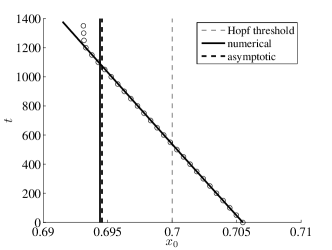
(a) $x_{0}$ versus $t$

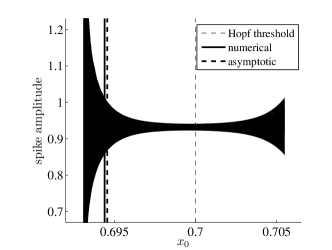
(b) amplitude of oscillation versus $t$

Figure 11: In the left figure, the curve represents the asymptotic prediction for the spike location given by (3.9), while the circles were obtained by numerically solving the PDE system (3.1). The deviation beginning near $t=1200$ is due to oscillations growing beyond the asymptotic regime. Note that the deviation occurs well after the Hopf bifurcation (vertical dashed line). In the right figure, we show the corresponding oscillations in spike amplitude. The initial decay in the amplitude reflects the initial stability of the solution. Near $x_{0}=0.7$ (vertical dashed line), a Hopf bifurcation occurs, at which point the spike oscillations begin to grow. When $x_{0}\approx 0.6944$ (heavy solid line), the oscillations grow to their original size. The asymptotic prediction is $x_{0}^{*}\approx 0.6946$ (heavy dashed line). Here, $(p,q,r,s)=(3,3,3,0)$, $\varepsilon=0.005$, $D=4$, and $\tau=0.891$.

In Figure 12, we show a case with the same parameters except with $\varepsilon=0.05$. The time scale of the drift is much faster in this case so that individual oscillations are visible. Further, the starting point may be set farther in the stable regime ($x_{0}(0)=0.75$) without danger of the oscillation amplitude becoming too small at a later time. However, the Hopf-bifurcation threshold is not as sharp due to larger $\varepsilon$, causing oscillations to begin growing at $x_{0}\approx 0.72$ instead of at $x_{0}\approx 0.7$ as in Figure 11(b) for smaller $\varepsilon$. As such, the predicted value of $x_{0}^{*}\approx 0.6492$ is rather far from the numerical value of $0.6923$ (heavy solid). The delay in bifurcation is still evident, as the spike must move well past the (numerical) bifurcation point before the bifurcation is fully realized. This illustration shows the difficulty in balancing the small $\varepsilon$ required for asymptotic accuracy and the larger $\varepsilon$ required for numerical workability.

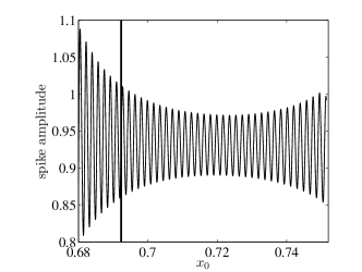
Figure 12: The same parameters as in Figure 11 except with $\varepsilon=0.05$. Due to larger $\varepsilon$, the Hopf bifurcation is triggered at $x_{0}\approx 0.72$ before the spike reaches the theoretical threshold of $x_{H}\approx 0.7$. The Hopf bifurcation is then fully realized at $x_{0}\approx 0.6923<0.72$ (heavy vertical line) when the oscillations return to their original amplitude. The asymptotic result of $x_{0}^{*}=0.6492$ is not shown.

In Figure 13(a), we compile results for $\varepsilon=0.007$ (circles) and $\varepsilon=0.005$ (squares) for various starting locations $x_{0}(0)$. The curve represents the asymptotic result show in Figure 10. We observe good agreement between asymptotic and numerical results, with the results for $\varepsilon=0.005$ appearing to yield closer agreement. In Figure 13(b), we show similar results for $(p,q,r,s)=(3,2,3,0)$ and $\varepsilon=0.005$. Because the character of oscillations at the beginning appeared slightly different from that of Figure 11(b), we defined the numerical result for $x_{0}^{*}$ in a slightly different manner. However, the delay effect, illustrated by the increasing relation between $x_{H}-x^{*}$ and $x_{0}(0)-x_{H}$, is still evident and agreeable with asymptotic results.

(a) $(p,q,r,s)=(3,3,3,0)$

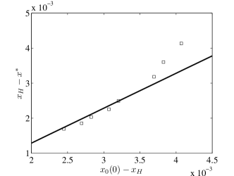
(b) $(p,q,r,s)=(3,2,3,0)$

Figure 13: In the left figure, we compare the asymptotic prediction (solid line) for the delay with the numerical results. The circles (squares) indicate results for $\varepsilon=0.007$ ($\varepsilon=0.005$). The Hopf bifurcation occurs when $x_{0}=x_{H}\approx 0.7$. The spike is stable (unstable) when $x_{0}>x_{H}$ ($x_{0}<x_{H}$). Oscillations return to their initial amplitude when $x_{0}=x_{0}^{*}<x_{H}$. While results for both values of $\varepsilon$ follow the trend of the asymptotic result, the results for $\varepsilon=0.005$ show better agreement. Here, $(p,q,r,s)=(3,3,3,0)$, $D=4$, and $\tau=0.891$. In the right figure, we show similar results for $(p,q,r,s)=(3,2,3,0)$, $\varepsilon=0.005$, $D=4$, and $\tau=0.5$.

Finally, we give an example of a scenario where $\tau_{H}(x_{0})$ is non-monotonic, as in Figure 3(b). Qualitatively, the theory suggests that the larger $x_{0}(0)-x_{H}$ is, the farther into the unstable zone the spike can penetrate before the Hopf bifurcation is fully realized. Figure 3(b) shows that, for appropriate $\tau$ and $x_{0}(0)$ sufficiently large, it is possible for $\psi$ never to reach 0 in the unstable zone. In such a case, no solution for $x_{0}^{*}$ of (3.14) would exist. That is, if the spike starts far enough into the stable zone to the right of $x_{Hsu}$, it may pass safely through the unstable zone $x_{0}\in(x_{Hus},x_{Hsu})$ without the Hopf bifurcation ever being fully realized.

The theory is illustrated in Figure 14 for $(p,q,r,s)=(3,3,3,0)$, $\varepsilon=0.005$, $D=1$, and $\tau=1.245$. The three colors differ only in the starting location $x_{0}(0)$. In the red plot, starting closest to the bifurcation threshold, oscillations initially decay while the spike is in the stable regime. Upon crossing $x_{Hsu}$ into the unstable regime, the oscillations grow to beyond their original value. In this case, the Hopf bifurcation has been fully realized before the spike has passed through the unstable zone. Upon crossing $x_{Hus}$ into the stable regime, the oscillations then decay. The purple plot shows that starting farther into the stable zone reduces the maximum oscillation amplitude attained in the unstable zone. However, the amplitude still exceeds its original value while in the unstable zone. The blue plot shows that starting sufficiently far in the stable regime allows the spike to pass safely through the unstable zone without the Hopf bifurcation being fully realized. This behavior may be explained by noting in Figure 14 that the farther into the stable regime the spike is initially set, the more the oscillation amplitude has decayed by the time the Hopf bifurcation is triggered, thus requiring more time in the unstable zone to recover to its original value. We have shown in this scenario that the phenomenon of delay makes it possible to pass safely through an unstable regime into a stable zone.

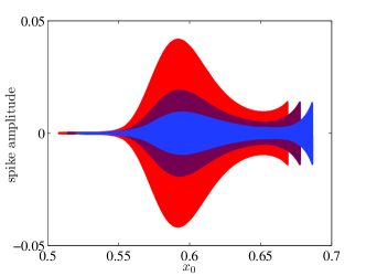
Figure 14: Plots of spike amplitude versus $x_{0}$ with $(p,q,r,s)=(3,3,3,0)$, $\varepsilon=0.005$, $D=1$, and $\tau=1.245$. The three colors differ only in the starting location $x_{0}(0)$. In the red plot, starting closest to the bifurcation threshold, oscillations grow in the unstable regime to beyond their original value. In this case, the Hopf bifurcation is fully realized before the spike passes through the unstable zone. The purple plot shows that starting farther into the stable zone reduces the maximum oscillation amplitude attained in the unstable zone. Starting even farther back, the blue plot shows that the spike may pass safely through the unstable zone without the oscillation amplitude ever reaching its original value.

In the next section, we consider the delay of a monotonic competition instability of a two boundary spike equilibrium solution in a generalized Gray-Scott model. Unlike the GM model, the Gray-Scott model exhibits a saddle node structure associated with weak dynamics just beyond the saddle. Analogous to the second scenario just considered, by introducing sufficient delay into the system through careful choice of initial conditions, we find that the weak saddle node dynamics may dominate the dynamics of the more dominant competition instability.

4   Example 3: Competition instability of a two boundary spike solution

For this example, we consider a two boundary spike solution of the generalized Gray-Scott (GS) model

$$v_{t}=\varepsilon^{2}v_{xx}-v+Auv^{3}\,,\qquad-1<x<1\,,\qquad v_{x}(\pm 1,t)=0\,,\qquad t>0\,,$$ (4.1a)

$$\tau u_{t}=Du_{xx}+(1-u)+\frac{1}{\varepsilon}uv^{3}\,,\qquad-1<x<1\,,\qquad u_{x}(\pm 1,t)=0\,,\qquad t>0\,.$$ (4.1b)

As in the previous examples, the diffusivity $\varepsilon^{2}$ of the activator component ($v$) is asymptotically small compared to the diffusivity $D$ of the inhibitor component ($u$). The $uv^{3}$ nonlinearity replaces the usual $uv^{2}$ term, and leads to an explicitly solvable NLEP. In this rescaled form of the GS model, the parameter $A$ is referred to as the feed-rate parameter, as it is a measure of how strongly the inhibitor is fed into the system from an external reservoir. In the context of solutions characterized by spikes in the activator component, if the feed-rate $A$ is too small, the process that fuels the activator spikes becomes insufficient, and one or more spikes collapse monotonically in time. In Figure 4(a), we show a two boundary spike equilibrium solution of (4.1) for $v(x)$ (solid) and $u(x)$ (dashed, and scaled by a factor of $6$ to facilitate plotting). The two spikes are of equal amplitude, are stable to slow drift instabilities, and remain centered at $x=\pm 1$ for all time. Figure 4(b) plots their amplitudes as $A$ is decreased past a stability threshold at which the feed-rate becomes insufficient to support two spikes. Note that the collapse of the left spike (light solid) is monotonic in time.

This type of instability, referred to as a competition instability due the local conservation of spike amplitudes at onset, occurs when a single eigenvalue crosses into the right-half plane through the origin. This is in contrast to the Hopf-bifurcations studied in the previous sections, where two complex conjugate eigenvalues crossed through the imaginary axis, leading to an oscillatory instability. As $A$ is decreased sufficiently past the competition threshold $A_{-}$, the solution encounters a saddle node bifurcation at $A=A_{m}<A_{-}$, past which point the two boundary spike solution ceases to exist. An example of the saddle node structure is shown in Figure 5. On the upper branch, the heavy solid segment indicates stable solutions. The light solid segment indicates solutions unstable to the competition mode. The stability transition occurs at $A=A_{-}\approx 4.6351$, while the saddle node occurs at $A=A_{m}\approx 4.6206$. The arrow indicates the evolution of the spike amplitude as $A$ is decreased. The lower branch is always unstable, and will not be considered.

As in the previous two sections, because $A$ starts in the stable regime $A>A_{-}$, a delay is expected to occur such that the competition instability is fully realized only when $A$ has been decreased sufficiently past $A_{-}$ to $A=A^{*}<A_{-}$. This gives rise to the two scenarios, $A^{*}>A_{m}$ and $A^{*}<A_{m}$. In the first scenario, the instability fully sets in before the system reaches the saddle node so that the solution has been driven relatively far from equilibrium by the instability. In the second scenario, the instability does not fully set in, leaving the solution still very close to equilibrium when it reaches the saddle node. These two scenarios differ markedly in their response to amplitude perturbations slightly past the saddle node. We illustrate both of these scenarios numerically in later sections. We note that, since no solution exists below $A=A_{m}$, the statement $A^{*}<A_{m}$ only serves to state that the instability is not expected to set in before the system reaches the saddle node. No quantitative predictions of delay can be made in this case.

In what follows, we take $A$ to be the bifurcation parameter, and study the delay that occurs as it is slowly decreased through the competition threshold. The parameters $D$ and $\tau$ remain constant. In the analysis, $\tau$ is set to $0$ while in the numerical computations of §4.2, $\tau$ is taken to be a value much smaller than one. We begin by first stating the two boundary spike solution and deriving values for $A_{m}$, $A_{-}$, and the expected delay $A_{-}-A_{*}$. As in the previous sections, we present only key steps of the analysis. Full derivations may be found in Appendix C.

4.1   Two boundary spike equilibrium and prediction of delay

For constant $A$, the two boundary spike equilibrium solution of (4.1) is

$$v_{e}\sim\frac{1}{\sqrt{AU_{-}}}w\left(\varepsilon^{-1}(x+1)\right)+\frac{1}{\sqrt{AU_{-}}}w\left(\varepsilon^{-1}(x-1)\right)\,,\qquad u_{e}\sim 1-\frac{b}{A^{3/2}U_{-}^{1/2}}G(x)\,,$$ (4.2)

where $w(y)$ and $G(x)$ are given by

$$w(y)=\sqrt{2}\operatorname{sech}y\,;\qquad\int_{-\infty}^{\infty}\!w^{3}\,dy\equiv b=\pi\sqrt{2}\,,\qquad G(x)=\frac{(\theta_{0}/2)\cosh(\theta_{0}x)}{\sinh\theta_{0}}\,.$$

In (4.2), $0<U_{-}<1/3$ is the smaller solution of the equation

$$H(U)\equiv\sqrt{U}(1-U)=\frac{b}{A^{3/2}}G(0)\,.$$ (4.3)

The upper branch in Figure 5 is a plot of the spike amplitude $\sqrt{2/(AU_{-})}$ as a function of $A$, while the bottom is a plot of $\sqrt{2/(AU_{+})}$, where $1/3<U_{+}<1$ is the larger solution of (4.3). To compute the value of $A$ at the saddle point, we note that $H(U)$ in (4.3) has a global maximum at $U=1/3$ where $H(1/3)=2/(3\sqrt{3})$. For a solution to (4.3) to exist, $A$ must satisfy $A>A_{m}$, where $A_{m}$ is the value at the saddle given by

$$A_{m}=\left[\frac{3\sqrt{3}\,b\,G(0)}{2}\right]^{2/3}\,.$$ (4.4)

Here, $G(x)$ is defined in (4.2).

To determine the stability of (4.2) for constant $A$, we perturb the equilibrium by

$$v=v_{e}+e^{\lambda t}\phi\,,\qquad u=u_{e}+e^{\lambda t}\eta\,;\qquad\phi,\eta\ll 1\,.$$ (4.5)

With $\tau=0$, two modes of instability are possible corresponding to odd and even eigenfunction $\phi$. The odd competition mode satisfies $\phi(x)=-\phi(-x)$ and $\eta(x)=-\eta(-x)$. As described above, the competition instability leads to the growth of one spike at the expense of the collapse of the other. The even mode, referred to as the synchronous mode, satisfies $\phi\,^{\prime}(0)=\eta\,^{\prime}(0)=0$ with $\phi(x)=\phi(-x)$ and $\eta(x)=\eta(-x)$. The synchronous mode leads to the simultaneous collapse of both spikes. In Appendix C, we show that the lower branch is always unstable to both modes of instability, while the upper branch is always stable to the synchronous mode. We now obtain the condition for which the upper branch is stable to the competition mode.

For $\tau=0$, we obtain from the explicitly solvable NLEP

$$\lambda=3-\frac{9}{2\left[1+\frac{U^{3/2}}{H(U)}\coth^{2}\theta_{0}\right]}\,.$$ (4.6)

The condition $\lambda=0$ yields that, at the competition instability threshold,

$$U_{-}=1-\frac{1}{1+C}\,\equiv\,U_{e-}\,;\qquad C\equiv\frac{1}{2\coth^{2}\theta_{0}}\,,$$ (4.7)

with $\lambda<0$ ($\lambda>0$) when $U_{-}<U_{e-}$ ($U_{-}>U_{e-}$). We note that, with $C<1/2$ for all $\theta_{0}>0$, we have that $0<U_{e-}<1/3$, corresponding to a solution on the upper branch of Figure 5. The lower branch is thus always unstable to the competition mode. As $D\to 0$, $\theta_{0}=1/\sqrt{D}\to\infty$ so that $U_{e-}\to 1/3$. Thus, on an infinitely long domain, the entire upper branch is always stable to both modes of instability. The stability to the competition mode on an infinite domain may be interpreted as the lack of a “crowding out” effect between the spikes. That is, the larger the domain size (or similarly, the smaller the value of $D$), the weaker is the interaction between the spikes, and the greater the number of spikes that may co-exist. For this reason, the competition instability is sometimes referred to as an “overcrowding” instability. With $A_{m}$ defined in (4.4), we have from (4.3) that the value of $A$ at the competition threshold is given by

$$A_{-}=A_{m}\left[\frac{3\sqrt{3}H(U_{e-})}{2}\right]^{-2/3}\,,$$ (4.8)

with $U_{e-}$ given in (4.7). As the bifurcation diagram in Figure 5 suggests, $\lambda<0$ ($\lambda>0$) when $A>A_{-}$ ($A<A_{-}$).

We note that, had we considered the case of two interior spikes for $v_{e}$ and $u_{e}$, the spectrum of the linearized equation for $\phi$ and $\eta$ would also contain small eigenvalues of $\mathcal{O}(\varepsilon^{2})$. The largest of these eigenvalues is associated with a slow drift instability, with corresponding eigenfunctions $\phi$ and $\eta$ being locally odd about the center of the spikes. It can be shown that the drift instability threshold occurs at a larger value of $A$ than does the competition threshold. As $A$ decreases past $A_{-}$, it must then first trigger the drift instability. By considering spikes located at the two boundaries where we impose pure Neumann conditions, drift instabilities are eliminated. Doing so made the numerical validations significantly less difficult.

To calculate the delay that results from slowly decreasing $A$ past $A_{-}$ according to,

$$A=A_{0}-\xi\,;\qquad A_{0}>A_{-}\,,\qquad\xi=\varepsilon t\,,$$ (4.9)

we replace (4.5) by the WKB ansatz

$$v=v_{e}+e^{\frac{1}{\varepsilon}\psi(\xi)}\phi\,,\qquad u=u_{e}+e^{\frac{1}{\varepsilon}\psi(\xi)}\eta\,;\qquad\phi,\eta\ll 1\,.$$

As in the previous two examples, we draw the equivalence $\psi^{\prime}=\lambda$, from which we obtain

$$\psi(A)=\int_{0}^{\xi}\!\lambda\,d\xi=-\int_{A_{0}}^{A}\!\lambda(A)\,dA\,,$$ (4.10)

where we set $\psi(0)=0$ and have used (4.9) to change the variable of integration from $\xi$ to $A$. In (4.10), $\lambda(A)$ may be obtained by explicitly solving (4.3) for $U(A)$, and using $U(A)$ in (4.6). Since $\lambda<0$ when $A>A_{-}$, $\psi$ will be negative and decreasing until $A$ is decreased to $A_{-}$. At $A=A_{-}$, $\psi$ will begin to increase, reaching $0$ only when $A=A^{*}<A_{-}$. We define $A^{*}$ as the value of $A$ at which the competition instability has fully set in.

Setting $\psi(A^{*})=0$ in (4.10) and solving the resulting algebraic equation for $A^{*}<A_{-}$, we obtain a relation between the delay $A_{-}-A^{*}$ and the “initial buffer” $A_{0}-A_{-}$. An example of a typical relationship is shown in Figure 15(a) for $D=3$. Note that, as in §2.1 and §3.1, the delay in terms of $A$ are independent of the rate at which it is decreased. The increasing function shows that, the larger the initial buffer, the larger the expected delay. The values of $A_{0}$ in Figure 15(a) are such that $A^{*}>A_{m}$ so that the instability sets in before the system reaches the saddle node. In Figure 15(b) we plot, for various $D$, $A_{m}$ (solid), $A_{-}$ (dashed), and the starting value of $A_{0}=A_{0}^{m}$ (dash-dotted) such that $A^{*}=A_{m}$. For $A_{0}<A_{0}^{m}$, the systems starts sufficiently close to threshold such that the delay is expected to be small and the instability sets in before $A$ reaches its saddle value $A_{m}$. This is illustrated schematically as scenario 1 in Figure 15(b), where the arrow ending above the $A_{m}$ curve indicates that the instability sets in before $A_{m}$. When $A_{0}>A_{0}^{m}$, the delay increases to the point where the instability does not fully set in by the time $A=A_{m}$. This is illustrated as scenario 2 in Figure 15(b). Here, the arrow extends below $A_{m}$, with the dotted segment indicating the delay that may have occurred in the absence of a saddle. In the next section, we show that the asymptotic prediction in Figure 15(a) agrees with results obtained by numerically solving (4.1). We also highlight the differences between scenarios 1 and 2.

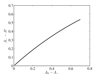
(a) $A_{-}-A^{*}$ versus $A_{0}-A_{-}$

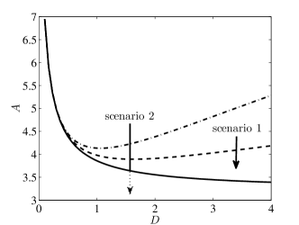
(b) $A_{0}^{m}$ versus $D$

Figure 15: In the left figure, we show the expected delay $A_{-}-A^{*}$ as a function of the initial buffer $A_{0}-A_{-}$ for $D=3$ and $\tau=0$. The increasing function indicates that the larger the initial buffer, the larger the expected delay. In the right figure we plot, as functions of $D$, $A_{m}$ (solid), $A_{-}$ (dashed), and $A_{0}^{m}$ (dash-dotted), where $A_{0}^{m}$ is the starting value of $A$ for which $A^{*}=A_{m}$. If $A_{0}<A_{0}^{m}$ (scenario 1), the delay sets in before $A_{m}$. If $A_{0}>A_{0}^{m}$ (scenario 2), the delay does not set in by the time $A$ has decreased to $A_{m}$.

4.2   Numerical validation

In this section, we illustrate the theory of §4.1 by numerically solving the PDE system (4.1) with $A$ taken to be the slowly decreasing function of time given in (4.9). The parameter $\tau$ was taken to be a small positive number much less than one. The time integration was performed using the MATLAB pdepe() routine. The initial conditions were taken as a perturbation of a true equilibrium state $(v(x,0),u(x,0))$ = $(v_{e}^{*}(x),u_{e}^{*}(x))$,

$$v(x,0)=v_{e}^{*}(x)\left(1-\delta\operatorname{sech}(\varepsilon^{-1}(x+1))+\delta\operatorname{sech}(\varepsilon^{-1}(x-1))\right)\,,\qquad u(x,0)=u_{e}^{*}(x)\,;\qquad 0<\delta\ll 1\,.$$ (4.11)

The equilibrium state $(v_{e}^{*}(x),u_{e}^{*}(x))$ was computed by integrating (4.1) to equilibrium starting from (4.2). The perturbation in (4.11) decreases the amplitude of the spike centered at $x=-1$, and increases by an equal amount that of the spike centered at $x=1$. We begin with an example of scenario 1 with $A_{0}<A_{0}^{m}$.

In Figure 16(a), we show the same typical result with $\varepsilon=0.004$ and $D=3$ as in Figure 4(b) except with $A(t)$ plotted on the horizontal axis. Note that, since $A$ is a decreasing function of time, the direction of time increase is to the left. As $A$ decreases, both amplitudes decrease as indicated by Figure 5. The stability threshold $A^{-}$ is indicated by the vertical dotted line, the asymptotic prediction of $A^{*}$ by the vertical dashed line, and the numerical value of $A^{*}$ by the vertical solid line. We observe good agreement between the asymptotic prediction and numerical value of $A^{*}$. As predicted, the amplitudes do not appear to diverge until $A\approx A^{*}$, well after the instability has been triggered. This illustrates the delay in competition instability. The instability then leads to the eventual collapse of the left spike along with the growth in amplitude of the right spike. The amplitude of the remaining spike continues to decrease with the continued decrease of $A$.

In Figure 16(b), we illustrate the phenomenon more clearly by plotting the difference in amplitudes as a function of $A$. The vertical lines correspond to those in Figure 16(a). When $A>A_{-}$, the system is stable, causing the initial perturbation to decay and the amplitudes to grow closer together. When $A=A_{-}$, the instability is triggered and the amplitudes begin to diverge. However, since the amplitudes grew closer together on the interval $A_{0}\geq A>A_{-}$, $A$ must be decreased well beyond $A_{-}$ for the amplitude difference to grow back to its initial size at $t=0$. For $D=3$, we find from Figure 15(b) that $A_{-}\approx 4.03$, which matches almost exactly the location of the minimum in Figure 16(b), indicating again excellent agreement between between asymptotic and numerical results.

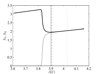
(a) spike amplitudes versus $A$

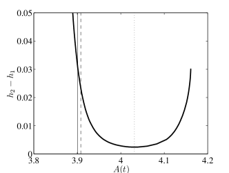
(b) amplitude difference versus $A$

Figure 16: In the left figure, we plot the amplitude of the left (light solid) and right (heavy solid) spikes as a function of $A$, with $A$ being decreased according to (4.9). Increasing time is to the left. The stability threshold $A_{-}$ is indicated by the vertical dotted line, the asymptotic prediction of $A^{*}$ by the vertical dashed line, and the numerical value of $A^{*}$ by the vertical solid line. The amplitude difference is plotted in the right figure, with the vertical lines corresponding to those in the left figure. Starting at $A_{0}>A_{-}$, the amplitudes grow closer together until the stability threshold $A=A_{-}\approx 4.03$ is reached. Here, $A_{-}$ is computed using (4.8). For $A<A_{-}$, the solution enters the unstable regime, causing the amplitudes to diverge. The difference in amplitudes does not reach their original value until well after $A=A_{-}$, indicating delay.

We repeat the computations with $D=3$ and find the delay for various values of the initial buffer. The results are compiled in Figure 17, where we compare the results to asymptotic result of Figure 15(a) for $\varepsilon=0.008$ (circles) and $\varepsilon=0.004$ (squares). We observe excellent agreement, with the numerical results for $\varepsilon=0.004$ matching the asymptotic result (solid curve) more closely for small $A_{0}$. The deviation of the squares from the curve for larger $A_{0}$ is likely due to the small $\mathcal{O}(e^{-1/\varepsilon})$ amplitude difference being obscured by numerical errors.

Figure 17: Comparison of numerical and asymptotic (solid) results for $D=3$ and $\varepsilon=0.008$ (circles) and $\varepsilon=0.004$ (squares). The results for $\varepsilon=0.004$ match the asymptotic result (solid curve) more closely for small $A_{0}$. The deviation of the squares from the curve for larger $A_{0}$ is likely due to the small $\mathcal{O}(e^{-1/\varepsilon})$ amplitude difference being obscured by numerical errors.

To illustrate the second scenario where $A^{*}<A_{m}$, we first confirm numerically the location of the saddle. To do so, we solve (4.1) on the domain $0<x<1$ with pure Neumann boundary conditions for one boundary spike centered at $x=1$. In this way, we eliminate the possibility of the odd competition instability and isolate the effects of the saddle node. In Figure 18(a), we show the evolution of the spike amplitude as $A$ is decreased starting from a true one boundary spike equilibrium, analogous to $(v_{e}^{*}(x),u_{e}^{*}(x))$, with $D=0.4$ and no initial perturbations. The heavy solid curve shows the case where the decrease of $A$ is stopped at $A=A_{m}+0.004$, slightly before it reaches its value at the saddle. The value for $A_{m}\approx 4.6206$ may be computed from (4.4) and is indicated by the vertical dashed line. As shown in Figure 18(b), the spike amplitude settles to a constant non-zero value after the time that the decrease of $A$ has ceased (heavy dashed line). The light solid curves in Figures 18(a) and 18(b) show the case where $A$ is decreased slightly past the saddle to $A=A_{m}-0.004$. Contrary to the first case, the spike collapses after the decrease of $A$ has ceased (light dashed line in Figure 18(b)). We thus conclude that the true location of the saddle is close to that predicted by the asymptotic result (4.4), and that in a two-spike equilibrium, the dynamics beyond the saddle induce the simultaneous collapse of both spikes. We emphasize that the simultaneous collapse is due to the effect of the saddle, not the synchronous instability described in §4.1.

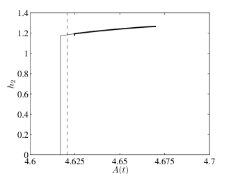
(a) spike amplitude versus $A$

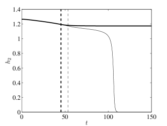
(b) spike amplitude versus $t$

Figure 18: Evolution of the amplitude of a one boundary spike quasi-equilibrium solution as $A$ is slowly decreased. In the left figure, we plot the amplitude of the spike as a function of $A$. The saddle value $A_{m}\approx 4.6206$ is indicated by the vertical dashed line. In the case that $A$ stops decreasing at $A=A_{m}+0.004$ (heavy solid curve), the spike settles to a constant non-zero value. If $A$ is decreased past $A_{m}$ to $A=A_{m}-0.004$, the spike collapses. The corresponding evolution as a function of time is shown in the right figure. The heavy (light) dashed line indicates the time that $A$ reaches its terminal value of $A_{m}+0.004$ ($A_{m}-0.004$). The starting value of $A$ in both instances is $A_{0}=4.6701$. Here, $\varepsilon=0.001$, and $D=0.4$.

We now contrast the two scenarios $A_{0}<A_{0}^{m}$ and $A_{0}>A_{0}^{m}$. Recall that if $A_{0}<A_{0}^{m}$, the instability is expected to set in before $A$ reaches the saddle, while if $A_{0}>A_{0}^{m}$, the delay is sufficiently large so that the instability does not fully set in when $A$ reaches $A_{m}$. When two spikes are present, two competing effects take place slightly beyond the saddle node. The less dominant effect is that just described, which leads to the simultaneous collapse of both spikes. The more dominant is the residual effect of the competition instability, which leads to the collapse of one spike and the growth of the other.

The relative dominance may be attributed to the zero eigenvalue of the synchronous mode exactly at the saddle node. Recall that the lower solution branch is always unstable to the even synchronous mode while the upper branch is always stable to the even synchronous mode. Where they meet, the eigenvalue of the even mode must be zero. While no spike solutions exist beyond the saddle, the dynamics associated with an even perturbation will be slow due to the nearby presence of the zero eigenvalue. Similarly, the dynamics associated with an odd perturbation will be relatively fast due to the nearby presence of the positive eigenvalue of the competition mode.

We therefore expect for a two spike solution that when $A$ is decreased to below $A_{m}$, perturbing the solution with both an odd and even perturbation would result in dynamics mirroring that of the dominant competition instability. One spike would collapse while the other would survive. This is depicted as scenario 1 in Figure 19(a), where $A_{0}<A_{0}^{m}$. On the left vertical axis, we plot the amplitude of the left (light solid) and right (heavy solid) spikes as $A$ is decreased, stopping at $A=A_{m}-0.004$, slightly off the saddle. On the right vertical axis, we plot the amplitude difference (dashed). The horizontal axis is time. The simultaneous decrease in both amplitudes at $t\approx 25.4$ is a result of an even perturbation added when $A$ reaches its terminal value of $A=A_{m}-0.004$. As expected, because the competition instability sets in before $A$ reaches $A_{m}$, the dynamics of the competition mode dominate beyond the saddle and only one spike collapses.

If the size of the odd perturbation were to be sufficiently small relative to that of the even, the slower growth of the even mode would be compensated for by its larger initial size. We would then expect the resulting dynamics to reflect that of the one spike solution, with both spikes collapsing almost simultaneously. This is depicted as scenario 2 in Figure 19(b), where $A_{0}>A_{0}^{m}$. As shown by the dashed curve, the instability has not fully set in by the time the $A$ reaches $A_{m}-0.004$ and the even perturbation is added. As a result, the even mode added at $t\approx 53.4$ dominates, and both spikes collapse. The presence of the competition mode causes the right spike to collapse slightly more slowly than the left. This scenario illustrates that the dynamics of a comparatively weak mode may prevail over that of a dominant mode due solely to the phenomenon of delay.

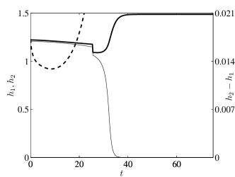
(a) scenario 1: $A_{0}=4.6451<A_{0}^{m}$

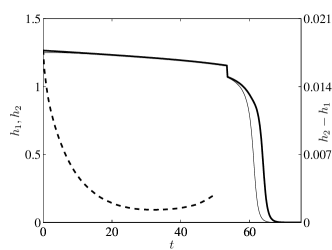
(b) scenario 2: $A_{0}=4.6701>A_{0}^{m}$

Figure 19: Plots of the amplitude of the left (light solid) and right (heavy solid) spikes versus time as $A$ is decreased from $A_{0}$ to $A_{m}-0.004$. For $D=0.4$, we find from Figure 15(b) that $A_{-}=4.6351$, $A_{m}=4.6206$, and $A_{0}^{m}=4.6534$. The near-vertical kinks at $t\approx 25.4$ in the left figure and $t\approx 53.4$ in the right are the result of the addition of an even perturbation when $A$ reaches $A_{m}-0.004$. The dashed curve, plotted against the right vertical axis, is a plot of the difference in spike amplitudes. In the left figure where $A_{0}<A_{0}^{m}$, the competition mode sets in early and dominates the dynamics near the saddle. As a result, only one spike collapses. In the right figure, the competition mode has not set in by the time the even perturbation is added. The resulting dynamics are near that of a simultaneous collapse of both spikes. The presence of the competition mode causes the right spike to collapse slightly more slowly than the left.

5   Discussion

We have presented three examples of delayed bifurcations for spike solutions of reaction-diffusion systems. In the first example with a single stationary spike, we considered the case where a model parameter $\tau$ was extrinsically tuned slowly past a Hopf bifurcation threshold. In the second example with a slowly drifting single spike, we studied the case where all model parameters were held constant and a Hopf bifurcation with $\mathcal{O}(1)$ time scale oscillations was triggered by intrinsic $\mathcal{O}(\varepsilon^{2})$ drift dynamics. A feature of this example not present in the first was that of a non-monotonic Hopf bifurcation threshold curve. Introducing sufficient delay into the system by careful selection of initial conditions, we found that the non-monotonicity allowed the spike to drift safely through a Hopf-unstable zone without the Hopf bifurcation fully setting in. In the third example with two stationary boundary spikes, we considered the delay of a competition instability as a feed rate parameter $A$ was tuned slowly past a stability threshold $A_{-}$. In addition to the competition threshold, there existed a saddle node bifurcation at $A=A_{m}$ past which no two-spike solutions exist. The presence of two critical values of $A$ led to two competing effects near the saddle node. We found that the delay played a critical role in determining which effect prevailed. In particular, we showed that a delay in the onset of the competition instability allowed the effect of the saddle node to dominate despite being comparatively weak.

In all three examples, linear stability analysis of the equilibrium or quasi-equilibrium solutions led to an explicitly solvable NLEP. By obtaining an explicit expression for the eigenvalue, we were able to formulate an algebraic problem for how far above a stability threshold the system must be in order for the instability to be fully realized. This delay in terms of the parameter was independent of the rate at which the system crossed the stability threshold. For all three examples, we solved the full PDE system numerically and observed excellent agreement with asymptotic predictions for the magnitude of delay. A key numerical challenge involved obtaining results not obscured by numerical errors when the system started far below threshold. For such computations, more digits of precision may be beneficial.

An interesting open problem in regards to Example 2 would be to understand the oscillations that occur well after the Hopf bifurcation has set in. For example, a weakly nonlinear theory may be developed to determine whether the bifurcation is subcritical or supercritical. In the case shown in Figure 11(b), we find that, well after the onset of the Hopf bifurcation, the oscillations exhibit a repeating pattern of series of five successively growing peaks, with peaks in each subsequent series slightly larger than the corresponding peaks in the previous series. This is shown in Figure 20.

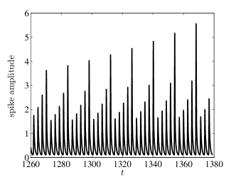
Figure 20: Nonlinear oscillations well after the intrinsically triggered Hopf bifurcations of Example 2 have set in. The parameters are the same as those of Figure 11(b). The oscillations exhibit a pattern of series of five successively growing peaks, with peaks in each subsequent series slightly larger than the corresponding peaks in the previous series. The oscillations also appear to be relaxational.

Another interesting problem would be to quantify the effect of a periodic forcing function on the delay of a Hopf bifurcation. For the ODE system considered in [2], it was found that a small amplitude sinusoidal forcing function with frequency equal to that of the Hopf frequency reduced the magnitude of the delay. For the example shown in Figure 11(b), we added to the right-hand side of (3.1a) a small forcing function $f(x,t)$ of the form

$$f(x,t)=0.001\sin(\omega_{H}t)\,w(\varepsilon^{-1}(x-x_{0}(t)))\,,$$

with $w(y)$ given in (3.5). Here, $\omega_{H}$ is the resonant Hopf frequency, and $x_{0}(t)$ is the center of the spike at time $t$. We observed in this case a beat phenomenon in the amplitude oscillations, with the low frequency envelope decaying in the Hopf stable region. Unlike that observed in [2], the forcing resulted in only a very slight decrease in the magnitude of delay. However, as part of a more detailed study of how delay varies with changes in forcing amplitude and frequency, the above result may help identify methods for more accurately determining bifurcation thresholds in experimental systems.

A related issue is the effect of noise on dynamics and bifurcations. In the context of ODE’s, a number of works elucidate the role that stochastic noise can play in pushing the system through tipping points; see for ex. [18, 19, 3, 20] and the references therein. Some recent papers also explore how the noise changes the dynamics in the context of stochastic PDE’s [21, 22, 23]. However much work remains to be done in this direction. In particular the effect of noise on the stability of spikes in RD systems remains largely unexplored.

Appendix A Construction and stability of a one-spike equilibrium of the GM model on the infinite line

Here, we construct a one-spike solution of (2.1) and derive an explicitly solvable nonlocal eigenvalue problem (NLEP) governing its stability to $\mathcal{O}(1)$ eigenvalues. Solving the NLEP, we derive (2.5) of §2. In the inner region of the spike centered at $x=0$, we transform to a stretched variable $y=x/\varepsilon$ and let

$$u\sim U(y)\,,\qquad v\sim V(y)\,.$$ (A.1)

The equilibrium problem on $-\infty<y<\infty$ is

$$V^{\prime\prime}-V+\frac{V^{3}}{U^{2}}=0\,,\qquad\frac{1}{\varepsilon^{2}}U^{\prime\prime}-U+\frac{V^{3}}{\varepsilon}=0\,,$$ (A.2)

with $V\to 0$ and $U$ bounded as $|y|\to\infty$. From (A.2) for $U$, we have to leading order that $U=U_{0}$ is a constant and

$$V=U_{0}w(y)\,,$$ (A.3)

where $w(y)$ is the homoclinic solution of

$$w^{\prime\prime}-w+w^{3}=0,\qquad-\infty<y<\infty\,,\qquad w(0)>0\,,\qquad w^{\prime}(0)=0\,,\qquad w\to 0\quad\mbox{as}\quad|y|\to\infty\,.$$ (A.4)

Equation (A.4) may be solved explicitly, with the solution given in (2.3).

In the outer region where $|x|=\mathcal{O}(1)$, the term $\varepsilon^{-1}v^{3}$ in (2.1b) is exponentially small. As $\varepsilon\to 0$, its mass becomes concentrated in an $\mathcal{O}(\varepsilon)$ width region around $x=0$ with height $\mathcal{O}(\varepsilon^{-1})$ at $x=0$. In the sense of distributions, using (A.1) and (A.3), we calculate $\varepsilon^{-1}v^{3}\to\left(\frac{1}{\varepsilon}\varepsilon\int_{-\infty}^{\infty}\!U_{0}^{3}w^{3}\,dy\right)\delta(x)=b\,U_{0}^{3}\delta(x)$, where $b$ is defined in (2.3), and $\delta(x)$ is the Dirac-delta function centered at $x=0$. Substituting this expression into (2.1b), we find that the outer solution for $u$ satisfies

$$u_{0xx}-u_{0}=b\,U_{0}^{3}\delta(x)\,,\qquad-\infty<x<\infty\,,\qquad u_{0}\to 0\quad\mbox{as}\quad|x|\to\infty\,,$$ (A.5)

with the matching condition $u_{0}(0)=U_{0}$. The solution to (A.5) is written in terms of a Green’s function $G(x;x_{0})$ as $u_{0}(x)=b\,U_{0}^{3}G(x;0)$, where where $G(x;0)$ satisfies

$$G_{xx}-G=-\delta(x)\,,\qquad-\infty<x<\infty\,,\qquad G\to 0\quad\mbox{as}\quad|x|\to\infty\,.$$ (A.6)

The solution to (A.6) is $G(x;0)={e^{-\lvert x\rvert}/2}$. Applying the matching condition $u_{0}(0)=U_{0}$, we calculate $U_{0}={1/\left(\sqrt{b\,G(0;0)}\right)}$. In this way, we obtain the results (2.2) and (2.3) of §2.

To derive the transcendental equation for the eigenvalue in (2.5), we linearize (2.1) by perturbing the equilibrium solution as in (2.4). The linearized equation is then

$$\lambda\phi=\varepsilon^{2}\phi_{xx}-\phi+\frac{3v_{e}^{2}}{u_{e}^{2}}\phi-\frac{2v_{e}^{3}}{u_{e}^{3}}\eta\,,\qquad-\infty<x<\infty\,,\qquad\phi\to 0\quad\mbox{as}\quad|x|\to\infty\,,$$ (A.7a)

$$\tau\lambda\eta=\eta_{xx}-\eta+\frac{3v_{e}^{2}}{\varepsilon}\phi\,,\qquad-\infty<x<\infty\,,\qquad\eta\to 0\quad\mbox{as}\quad|x|\to\infty\,.$$ (A.7b)

Here, $v_{e}$ and $u_{e}$ are given in (2.2). Since the coefficients $v_{e}^{2}/u_{e}^{2}$ and $v_{e}^{3}/u_{e}^{3}$ are localized near $x=0$, we seek solutions to (A.7a) where $\phi$ is localized near $x=0$ and $\eta$ varies over the same scale as does $u_{e}(x)$. With $\phi=\Phi(y)$ and $\eta(x)\sim\eta(0)$ as $x\to 0$, we obtain the following equation for $\Phi(y)$,

$$L_{0}\Phi-2w^{3}\eta(0)=\lambda\Phi\,,\qquad-\infty<y<\infty\,,\qquad\Phi\to 0\quad\mbox{as}\quad|y|\to\infty\,,$$ (A.8)

where the linear operator $L_{0}$ is defined as

$$L_{0}\psi\equiv\psi^{\prime\prime}-\psi+3w^{2}\psi\,.$$ (A.9)

To determine $\eta(0)$ in (A.8), we solve (A.7b) for $\eta(x)$. Since the term $v_{e}^{2}\phi$ is localized near $x=0$, we have in the sense of distributions that $\varepsilon^{-1}v_{e}^{2}\phi\sim\left[\int_{-\infty}^{\infty}\!U_{0}^{2}w^{2}\Phi(y)\,dy\right]\delta(x)$, where we have used (2.2) for $v_{e}$ in (A.7b). The resulting equation for $\eta(x)$ is then

$$\eta_{xx}-(1+\tau\lambda)\eta=-3U_{0}^{2}\left[\int_{-\infty}^{\infty}\!w^{2}\Phi\,dy\right]\delta(x)\,,\qquad-\infty<x<\infty\,,\qquad\eta\to 0\quad\mbox{as}\quad|x|\to\infty\,.$$ (A.10)

We write the solution to (A.10) in terms of the Green’s function $G_{\lambda}(x;0)$ as

$$\eta(x)\sim 3U_{0}^{2}\left[\int_{-\infty}^{\infty}\!w^{2}\Phi\,dy\right]G_{\lambda}(x;0)\,,$$ (A.11)

where $G_{\lambda}(x;0)$ satisfies

$$G_{\lambda xx}-(1+\tau\lambda)G_{\lambda}=-\delta(x)\,,\qquad-\infty<x<\infty\,,\qquad G_{\lambda}\to 0\quad\mbox{as}\quad|x|\to\infty\,.$$ (A.12)

The solution of (A.12) is

$$G_{\lambda}(x;0)=\frac{1}{2\sqrt{1+\tau\lambda}}e^{-\theta_{\lambda}\lvert x\rvert}\,,\qquad\theta_{\lambda}\equiv\sqrt{1+\lambda\tau}\,.$$ (A.13)

Using (A.11) to compute $\eta(0)$, and using $U_{0}={1/\left(\sqrt{b\,G(0;0)}\right)}$, we obtain the nonlocal eigenvalue problem (NLEP)

$$L_{0}\Phi-\chi w^{3}\frac{\int_{-\infty}^{\infty}\!w^{2}\Phi\,dy}{\int_{-\infty}^{\infty}\!w^{3}\,dy}=\lambda\Phi\,,\qquad\chi\equiv 6\frac{G_{\lambda}(0,0)}{G(0;0)}\,,$$ (A.14)

with $L_{0}\psi$ is defined in (A.9). From $G(0;0)={1/2}$ and (A.13), we calculate $\chi$ in (A.14) as

$$\chi=\frac{6}{\sqrt{1+\tau\lambda}}\,.$$ (A.15)

From [15], the specific choice of powers of the GM model in (2.1) allows the NLEP (A.14) to be solved explicitly. We begin by noting that, in addition to the zero eigenvalue with associated eigenfunction $w^{\prime}(y)$ that changes sign once on $-\infty<y<\infty$, $L_{0}\psi=\nu\psi$ has a unique positive eigenvalue $\nu_{0}=3$ with eigenfunction $\psi_{0}=w^{2}$ of constant sign. To show this, we first multiply (A.4) by $w^{\prime}$ and integrate to compute that $(w^{\prime})^{2}=w^{2}-{w^{4}/2}$. We then calculate

$$L_{0}w^{2}=2(w^{\prime})^{2}+2ww^{\prime\prime}-w^{2}+3w^{4}\,.$$ (A.16)

Then, by using (A.4) for $w^{\prime\prime}$ and the expression above for $w^{\prime}$, we find from (A.16) that indeed

$$L_{0}w^{2}=3w^{2}\,.$$ (A.17)

Next, we multiply (A.14) by $w^{2}$ and integrate over the real line to obtain

$$\int_{-\infty}^{\infty}\!w^{2}L_{0}\Phi dy=\chi\frac{\int_{-\infty}^{\infty}\!w^{5}dy\int_{-\infty}^{\infty}\!w^{2}\Phi dy}{\int_{-\infty}^{\infty}\!w^{3}dy}+\lambda\int_{-\infty}^{\infty}\!w^{2}\Phi dy\,.$$ (A.18)

With $\Phi(y)$, $\Phi^{\prime}(y)$, $w(y)$, and $w^{\prime}(y)$ all decaying exponentially to zero at infinity, Green’s second identity yields $\int_{-\infty}^{\infty}\!\Phi L_{0}w^{2}dy=\int_{-\infty}^{\infty}\!w^{2}L_{0}\Phi dy$. With this identity, together with (A.17), we obtain for the left-hand side of (A.18) that $\int_{-\infty}^{\infty}\!w^{2}L_{0}\Phi dy=3\int_{-\infty}^{\infty}\!\Phi w^{2}dy$. With this expression, the NLEP (A.18) then becomes

$$\int_{-\infty}^{\infty}\!\Phi w^{2}dy\left[3-\chi\frac{\int_{-\infty}^{\infty}\!w^{5}dy}{\int_{-\infty}^{\infty}\!w^{3}dy}-\lambda\right]=0\,.$$ (A.19)

Calculating $\int_{-\infty}^{\infty}\!w^{5}dy/\int_{-\infty}^{\infty}\!w^{3}dy=3/2$, we conclude that any eigenvalue of (A.14) for which the eigenfunction satisfies $\int_{-\infty}^{\infty}\!\Phi w^{2}dy\neq 0$ must satisfy the expression given in (2.5) of §2, where we use (A.15) for $\chi$ in (A.19).

Appendix B One-spike quasi-equilibrium and slow dynamics of the GM model on a finite domain

Here, we construct the one-spike quasi-equilibrium solution of (3.1) and derive the ODE (3.9) describing its slow dynamics. For the inner solution of a one-spike quasi-equilibrium solution centered at $x=x_{0}$, we let

$$u\sim U_{0}(y)+\varepsilon U_{1}(y)+\cdots\,,\qquad v\sim V_{0}(y)+\varepsilon V_{1}(y)+\cdots\,,\qquad y=\frac{x-x_{0}(\sigma)}{\varepsilon}\,;\qquad\sigma\equiv\varepsilon^{\alpha}t\,,$$ (B.1)

to obtain

$$V^{\prime\prime}-V+\frac{V^{p}}{U^{q}}=0\,,\qquad V\to 0\quad\mbox{as}\quad|y|\to\infty\,,$$ (B.2a)

$$\frac{1}{\varepsilon^{2}}DU^{\prime\prime}-U+\frac{1}{\varepsilon}\frac{V^{r}}{U^{s}}=0\,.$$ (B.2b)

The limiting conditions for (B.2b) come from matching conditions with the outer solution. From (B.2b), we have that $U\sim U_{0}$ is a constant to leading order so that $V_{0}$ satisfies

$$V_{0}^{\prime\prime}-V_{0}+\frac{V_{0}^{p}}{U_{0}^{q}}=0\,,\qquad V\to 0\quad\mbox{as}\quad|y|\to\infty\,.$$ (B.3)

The solution of (B.3) can be written

$$V_{0}\sim U_{0}^{\frac{q}{p-1}}w(y)\,,$$ (B.4)

where $w(y)$ is the solution of the equation in (3.4) with solution given in (3.5) of §3.

To compute the outer solution for $u=u_{0}(x)$ in (3.1b), we proceed as in Appendix A and represent the $v^{r}/u^{s}$ term as a weighted Dirac-delta function centered at $x=x_{0}$. We then have

$$Du_{0xx}-u_{0}=-U_{0}^{\frac{qr}{p-1}-s}b_{r}\,\delta(x-x_{0})\,,$$ (B.5)

where $b_{r}$ is defined in (3.5). The solution of (B.5) may be written in terms of a Green’s function $G(x;x_{0})$ as

$$u_{0}(x)=U_{0}^{\frac{qr}{p-1}-s}b_{r}G(x;x_{0})\,,$$ (B.6)

where $G(x;x_{0})$ satisfies

$$DG_{xx}-G=-\delta(x-x_{0})\,,\qquad G_{x}(\pm 1,x_{0})=0\,.$$ (B.7)

The solution of (B.7) is given by (3.6) of §3. The constant $G_{00}$ in (3.7) is found by imposing the jump condition $DG_{x}(x_{0}^{+};x_{0})-DG_{x}(x_{0}^{-};x_{0})=-1$. Finally, by imposing the matching condition $u(x_{0})=U_{0}$ in (B.6), we arrive at (3.8) of §3. With (B.4), (3.5), (B.6), and (3.6), the one-spike quasi-equilibrium is then given by (3.3).

To derive (3.9) for the drift of the spike center, we consider the next order in $\varepsilon$ of (B.2) with (B.1). We calculate that $dV_{0}/dt=-\varepsilon^{\alpha-1}V_{0}^{\prime}x_{0}^{\prime}$, while $dU_{0}/dt=\mathcal{O}(\varepsilon^{2})$. To match orders, we must take $\alpha=2$ so that $\sigma\equiv\varepsilon^{2}t$. We then have at the next order

$$LV_{1}\equiv V_{1}^{\prime\prime}-V_{1}+p\frac{V_{0}^{p-1}}{U_{0}^{q}}V_{1}=-V_{0}^{\prime}x_{0}^{\prime}+q\frac{V_{0}^{p}}{U_{0}^{q+1}}\,,$$ (B.8a)

$$DU_{1}^{\prime\prime}=-\frac{1}{U_{0}^{s}}V_{0}^{r}\,.$$ (B.8b)

By differentiating (B.3) with respect to $y$, we find that $LV_{0}^{\prime}=0$, or equivalently, $Lw^{\prime}=0$. The right-hand side of (B.8a) must then satisfy the solvability condition

$$\int_{-\infty}^{\infty}\!w^{\prime}\left[-x_{0}^{\prime}U_{0}^{R}w^{\prime}+qU_{0}^{Q}w^{p}U_{1}\right]\,dy=0\,;\qquad R\equiv\frac{q}{p-1}\,,\quad Q\equiv\frac{pq}{p-1}-q-1\,.$$ (B.9)

With $R-Q=1$ and $w^{\prime}w^{p}=(p+1)^{-1}dw^{p+1}/dy$, we have from (B.9)

$$x_{0}^{\prime}U_{0}\int_{-\infty}^{\infty}\!\left(w^{\prime}\right)^{2}\,dy=\frac{q}{p+1}\int_{-\infty}^{\infty}\!\left(w^{p+1}\right)^{\prime}U_{1}\,dy\,.$$ (B.10)

Integrating by parts once on the right-hand side of (B.10) and using that $w\to 0$ as $|y|\to\infty$, we obtain

$$x_{0}^{\prime}U_{0}\int_{-\infty}^{\infty}\!\left(w^{\prime}\right)^{2}\,dy=-\frac{q}{p+1}\int_{-\infty}^{\infty}\!w^{p+1}U_{1}^{\prime}\,dy\,.$$ (B.11)

Integrating by parts again on the right-hand side of (B.11) and letting $v(y)\equiv\int_{0}^{y}w^{p+1}\,ds$, we calculate

$$x_{0}^{\prime}U_{0}\int_{-\infty}^{\infty}\!\left(w^{\prime}\right)^{2}\,dy=-\frac{q}{p+1}\left[U_{1}^{\prime}v\bigg{\rvert}_{-\infty}^{\infty}-\int_{-\infty}^{\infty}\!vU_{1}^{\prime\prime}\,dy\right]\,.$$ (B.12)

Since $w^{p+1}$ is an even function and $v(0)=0$, we find that $v(y)$ is an odd function. Also, since $V_{0}^{r}$ is an even function, we have by (B.8b) that $U^{\prime\prime}$ is an even function. The integral term on the right-hand side of (B.12) therefore evaluates to 0. Now with $v(\infty)=-v(-\infty)$, we have from (B.12)

$$x_{0}^{\prime}=-\frac{q}{2(p+1)}K\frac{U_{1}^{\prime}(\infty)+U_{1}^{\prime}(-\infty)}{U_{0}}\,;\qquad K\equiv\frac{\int_{-\infty}^{\infty}\!w^{p+1}\,dy}{\int_{-\infty}^{\infty}\!\left(w^{\prime}\right)^{2}\,dy}\,.$$ (B.13)

The quantities $U_{1}^{\prime}(\pm\infty)$ may be calculated from the matching condition

$$U_{1}^{\prime}(\pm\infty)=u_{0x}(x_{0}^{\pm})\,,$$

yielding from (B.13)

$$x_{0}^{\prime}=-\frac{q}{2(p+1)}K\frac{1}{G_{00}}\left[G_{x}(x_{0}^{+};x_{0})+G_{x}(x_{0}^{-};x_{0})\right]\,,$$ (B.14)

where we have used (B.6) and (3.8) for $u_{0}$ and $U_{0}$, respectively. Using (3.6) and (3.7) in (B.14), we have

$$x_{0}^{\prime}=-\frac{q}{2(p+1)\sqrt{D}}K\left[\tanh\left(\theta_{0}(1+x_{0})\right)-\tanh\left(\theta_{0}(1-x_{0})\right)\right]\,.$$ (B.15)

The quantity $K$ in (B.15) is calculated in [15]. We include the calculation here for completeness. We first multiply (3.4) in §3 by $w^{\prime}$ and integrate to obtain

$$\frac{1}{2}\left(w^{\prime}\right)^{2}-\frac{1}{2}w^{2}+\frac{1}{p+1}w^{p+1}=C\,,$$ (B.16)

where $C=0$ since $w,w^{\prime}\to 0$ as $|y|\to\infty$. Integrating (B.16) over the entire real line yields

$$1-I_{1}+\frac{2}{p+1}K=0\,;\qquad I_{1}\equiv\frac{\int_{-\infty}^{\infty}\!w^{2}\,dy}{\int_{-\infty}^{\infty}\!\left(w^{\prime}\right)^{2}\,dy}\,.$$ (B.17)

To obtain a second equation involving $I_{1}$ and $K$, we multiply (3.4) by $w$, integrate by parts once on the $ww^{\prime\prime}$ term and apply the decay condition of $w$ to find

$$-1-I_{1}+K=0\,.$$ (B.18)

Solving (B.17) and (B.18) simultaneously, we find

$$K=\frac{2(p+1)}{p-1}\,.$$ (B.19)

Substituting (B.19) into (B.15), we obtain result (3.9) of §3. Because of the slow $\mathcal{O}(\varepsilon^{2})$ drift of the spike, analysis of $\mathcal{O}(1)$ time scale instabilities may be performed assuming a “frozen” spike centered at $x=x_{0}$. The analysis leading to an explicitly solvable NLEP then proceeds as in Appendix A and will not be included here. The reader may refer to [15] for details.

Appendix C Boundary spikes in the GS model and analysis of competition instability

Here, we construct the two boundary spike equilibrium (4.2) of (4.1) on the domain $x\in(-1,1)$. We then derive an NLEP and solve it to obtain thresholds of competition (given in (4.7)) and synchronous instabilities. To do so, we first construct a one-spike equilibrium centered at $x=1$ on $x\in(0,2)$, taking only the interval $(0,1)$. We then apply a reflection to obtain the two boundary-spike solution on the entire interval.

We let $x=\xi+1$ so that $-1<\xi<1$. The spike is then centered at $\xi=0$. The construction of the one-spike equilibrium then follows closely to that given in Appendix A. In the inner region with stretched variable $\zeta=\xi/\varepsilon$ and $u(\xi)\sim U_{0}(\zeta)$, $v(\xi)\sim V_{0}(\zeta)$, we find that $U_{0}$ is a constant while $V_{0}(\zeta)=w(\zeta)/\sqrt{AU_{0}}$, with $w(\zeta)$ given in (2.3). In the outer region, $u=u_{0}(\xi)$ satisfies

$$Du_{0\xi\xi}+(1-u_{0})=\frac{b}{A^{3/2}\sqrt{U_{0}}}\delta(\xi)\,,\qquad u_{\xi}(\pm 1)=0\,,$$ (C.1)

where the weight of the delta function is calculated in the usual way. Here, $b$ is defined in (2.3). The conditions $u_{\xi}(\pm 1)=0$ are correspond to even symmetry about $x=0$ in original coordinates. Note that the boundary conditions $u_{x}(\pm 1)=0$ are satisfied by the constant inner solution for $u$. The solution of (C.1) may be written $u_{0}(\xi)=1+\tilde{u(\xi)}_{0}$, where $\tilde{u}$ satisfies

$$\tilde{u}_{0}(\xi)=-\frac{b}{A^{3/2}\sqrt{U_{0}}}G(\xi;0)\,,$$ (C.2)

where $G(\xi;0)$ satisfies

$$DG_{\xi\xi}-G=-\delta(\xi)\,,\qquad G_{\xi}(\pm 1;0)=0\,.$$ (C.3)

The solution of (C.3) is

$$G(\xi;0)=G_{00}\left\{\begin{array}[]{lr}\frac{\cosh\left(\theta_{0}(\xi+1)\right)}{\cosh\theta_{0}}\,,&-1<\xi<0\,,\\ \frac{\cosh\left(\theta_{0}(\xi-1)\right)}{\cosh\theta_{0}}\,,&0<\xi<1\,,\end{array}\right.\,;\qquad G_{00}=\frac{1}{2\sqrt{D}\tanh\theta_{0}}\,,$$ (C.4)

where $\theta_{0}$ is defined in (3.7). The matching condition $u_{0}(0)=U_{0}$ determines $U_{0}$, yielding $U_{0}=1-bG(0;0)/(A^{3/2}\sqrt{U})$, which is equivalent to (4.3) of §4. The one spike equilibrium on $\xi\in(-1,1)$ is thus given by

$$v_{e1}(\xi)=\frac{1}{\sqrt{AU_{0}}}w\left(\varepsilon^{-1}\xi\right)\,,\qquad u_{e1}(\xi)=1+\tilde{u}_{0}(\xi)\,,$$ (C.5)

with $\tilde{u}_{0}$ given in (C.2).

On $x\in(0,1)$, the two boundary-spike solution is given by the the solution (C.5) on the interval $\xi\in(-1,0)$. That is, on $x\in(0,1)$, $u$ and $v$ are given by

$$v=\frac{1}{\sqrt{AU_{0}}}w\left(\varepsilon^{-1}(x-1)\right)\,,\qquad u=1-\frac{b}{A^{3/2}\sqrt{U_{0}}}\frac{\cosh\left(\theta_{0}x\right)}{2\sqrt{D}\sinh\theta_{0}}\,.$$ (C.6)

The solution on $x\in(-1,0)$ is an even reflection of (C.6) about $x=0$ so that $x\to-x$. Noting that $w(\zeta)$ and $\cosh x$ are both even functions, we obtain (4.2) with $U_{-}$ replaced by $U_{0}$. Here, $U_{0}$ is determined by the matching condition (4.3) and takes on the value $U_{-}$ or $U_{+}$ depending on whether the top or bottom solution branch is being considered.

To determine the stability of (4.2), we perturb the one-spike equilibrium on $\xi\in(-1,1)$ as

$$v=v_{e1}(\xi)+e^{\lambda t}\phi\,,\qquad u=u_{e1}(\xi)+e^{\lambda t}\eta\,;\qquad\phi,\eta\ll 1\,.$$ (C.7)

Here, $v_{e1}(\xi)$ and $u_{e1}(\xi)$ are the one-spike equilibrium solutions for $v$ and $u$ on $\xi\in(-1,1)$ given by (C.5). Substituting (C.7) in (4.1a) and (4.1b), we obtain the linearized system of equations

$$\lambda\phi=\varepsilon^{2}\phi_{\xi\xi}-\phi+3Au_{e1}v_{e1}^{2}\phi+Av_{e1}^{3}\eta\,,$$ (C.8a)

$$\tau\lambda\eta=D\eta_{\xi\xi}-\eta-\frac{1}{\varepsilon}\left[3u_{e1}v_{e1}^{2}+v_{e1}^{3}\eta\right]\,.$$ (C.8b)

The boundary conditions in $\xi$ for (C.8) depend on the mode of instability considered and is discussed below. In the inner region with the stretched variable $\zeta=\xi/\varepsilon$, we find from (C.8b) that $\eta=\eta_{0}$ is a constant to leading order. Note that this satisfies the no-flux conditions at $x=\pm 1$ in the original coordinates. Writing $\phi=\Phi(\zeta)$, we find that $\Phi$ satisfies

$$L_{0}\Phi+\frac{\eta_{0}}{\sqrt{A}U_{0}^{3/2}}w^{3}=\lambda\Phi\,,$$ (C.9)

where the operator $L_{0}$ is defined in (A.9). In (C.9), we have used (C.5) for $v_{e1}$ and the leading order behavior $u_{e1}\sim U_{0}$ for $u_{e1}$ in the inner region. The quantity $\eta_{0}$ must be obtained by solving the outer equation for $\eta(\xi)$.

In the outer region for (C.8b), we proceed as in Appendix A and represent the localized terms involving $\phi$ and $v_{e1}$ as appropriately weighted delta functions. In this way, we obtain the outer equation for $\eta$

$$D\eta_{\xi\xi}-(1+\tau\lambda)\eta=\left[\frac{b\eta_{0}}{\left(AU_{0}\right)^{3/2}}+\frac{3}{A}\int_{-\infty}^{\infty}\!w^{2}\Phi\,d\zeta\right]\delta(\xi)\,.$$ (C.10)

The competition mode of instability, which leads to the growth of one spike and the collapse of the other, is associated with an odd eigenfunction. We thus impose that $\eta(\pm 1)=0$ for the competition mode, which corresponds to $\eta(0)=0$ in the original $x$ coordinate. The synchronous mode, which leads to the collapse of both spikes, is associated with an even eigenfunction. This leads to the symmetry condition $\eta_{\xi}(\pm 1)=0$, which corresponds to $\eta_{x}(0)=0$ in the original $x$ coordinate. In imposing the boundary conditions at $\xi=\pm 1$, we implicitly assume the presence of image spikes centered at $\xi=\pm 2$.

For each mode, we define an associated Green’s function with appropriate boundary conditions

$$DG_{\pm\xi\xi}-(1+\tau\lambda)G_{\pm}=-\delta(\xi)\,,\qquad G_{+\xi}(\pm 1;0)=0\,,\qquad G_{-}(\pm 1;0)=0\,,$$ (C.11)

where $G_{+}$ ($G_{-}$) corresponds to the synchronous (competition) mode. The solution of (C.10) may then be written in terms of $G_{\pm}$ as

$$\eta(\xi)=-\left[\frac{b\eta_{0}}{\left(AU_{0}\right)^{3/2}}+\frac{3}{A}\int_{-\infty}^{\infty}\!w^{2}\Phi\,d\zeta\right]G_{\pm}(\xi;0)\,.$$ (C.12)

Finally, to find $\eta_{0}$, we apply the matching condition $\eta(0)=\eta_{0}$ in (C.12) and calculate

$$\eta_{0}=-\frac{\frac{3}{A}\int_{-\infty}^{\infty}\!w^{2}\Phi\,d\zeta}{\frac{1}{G_{\pm 00}}+\frac{b}{\left(AU_{0}\right)^{3/2}}}\,,$$ (C.13)

where $G_{\pm 00}\equiv G_{\pm}(0;0)$.

Now we may substitute (C.13) for $\eta_{0}$ into (C.9) to obtain

$$L_{0}\Phi-3w^{3}\frac{\int_{-\infty}^{\infty}\!w^{2}\Phi\,d\zeta}{b+\frac{(AU_{0})^{3/2}}{G_{\pm 00}}}=\lambda\Phi\,.$$ (C.14)

Using (4.3) in §4, we may write $A^{3/2}=bG_{00}/H(U_{0})$ so that we obtain from (C.14) the NLEP

$$L_{0}\Phi-\chi_{\pm}w^{3}\int_{-\infty}^{\infty}\!w^{2}\Phi\,d\zeta=\lambda\Phi\,,$$ (C.15)

where $\chi_{\pm}$ is defined as

$$\chi_{\pm}=\frac{3}{b\left(1+\frac{G_{00}}{G_{\pm 00}}\frac{U_{0}^{3/2}}{H(U_{0})}\right)}\,.$$ (C.16)

Here, $G_{00}$ is defined in (C.4). It was shown in Appendix A that the NLEP in (C.15) is explicitly solvable, yielding

$$\lambda=3-\frac{3}{2}\chi_{\pm}\,.$$ (C.17)

To complete the derivation of $\lambda$, we require $G_{\pm 00}$ in (C.16). The solutions for $G_{+}(\xi;0)$ and $G_{-}(\xi;0)$ in (C.11) are given by

$$G_{+}(\xi;0)=G_{+00}\left\{\begin{array}[]{lr}\frac{\cosh\left(\theta_{\lambda}(1+\xi)\right)}{\cosh\left(\theta_{\lambda}\right)}\,,&-1<\xi<0\,,\\ \frac{\cosh\left(\theta_{\lambda}(1-\xi)\right)}{\cosh\left(\theta_{\lambda}\right)}\,,&0<\xi<1\,,\end{array}\right.\,;\qquad G_{+00}=\frac{1}{2\sqrt{D}\sqrt{1+\tau\lambda}\tanh\theta_{\lambda}}\,,$$ (C.18)

and

$$G_{-}(\xi;0)=G_{-00}\left\{\begin{array}[]{lr}\frac{\sinh\left(\theta_{\lambda}(1+\xi)\right)}{\sinh\left(\theta_{\lambda}\right)}\,,&-1<\xi<0\,,\\ \frac{\sinh\left(\theta_{\lambda}(1-\xi)\right)}{\sinh\left(\theta_{\lambda}\right)}\,,&0<\xi<1\,,\end{array}\right.\,;\qquad G_{-00}=\frac{1}{2\sqrt{D}\sqrt{1+\tau\lambda}\coth\theta_{\lambda}}\,,$$ (C.19)

where $\theta_{\lambda}$ is defined in (A.13). Note that the parameter $\tau$ appears in the expressions only as $\tau\lambda$. Since we consider only monotonic instabilities, which occur as a single eigenvalue crosses into the right half-plane through the origin, any increase or decrease in $\tau$ cannot trigger such an instability. We may thus take $\tau=0$ for simplicity while also ensuring that no Hopf instabilities are present. With $\tau=0$, we have from (C.18) and (C.19)

$$\frac{G_{00}}{G_{+00}}=1\,,\qquad\frac{G_{00}}{G_{-00}}=\coth^{2}\theta_{0}\,.$$ (C.20)

Finally, using (C.20) in (C.16) and (C.17), we have the explicit expressions for the eigenvalues corresponding to the synchronous ($\lambda_{+}$) and competition modes ($\lambda_{-}$)

$$\lambda_{+}=3-\frac{9}{2\left[1+\frac{U_{0}^{3/2}}{H(U_{0})}\right]}\,,\qquad\lambda_{-}=3-\frac{9}{2\left[1+\frac{U_{0}^{3/2}}{H(U_{0})}\coth^{2}\theta_{0}\right]}\,.$$ (C.21)

Note that the expression for $\lambda_{-}$ in (C.21) is the same as that given in (4.6) of §4. Setting $\lambda_{-}=0$ yields the thresholds given in (4.7). Setting $\lambda_{+}=0$ in (C.21), we find that the stability threshold for the synchronous mode is $U_{0}=1/3$. Recalling that the upper branch corresponds to $0<U_{0}<1/3$ while the lower branch corresponds to $1/3<U_{0}<1$, we find that the threshold for the synchronous mode occurs at the saddle point, which was stated in §4. A simple calculation shows that the upper branch is always stable to the synchronous mode while the lower branch is always unstable.

Acknowledgements

T. Kolokolnikov and M. J. Ward gratefully acknowledge the grant support of NSERC. J. C. Tzou was supported by an AARMS Postdoctoral Fellowship.

References

- [1] P. Mandel, T. Erneux, The slow passage through a steady bifurcation: delay and memory effects, Journal of statistical physics 48 (5-6) (1987) 1059–1070.
- [2] S. M. Baer, T. Erneux, J. Rinzel, The slow passage through a hopf bifurcation: delay, memory effects, and resonance, SIAM Journal on Applied mathematics 49 (1) (1989) 55–71.
- [3] C. Kuehn, A mathematical framework for critical transitions: Bifurcations, fast–slow systems and stochastic dynamics, Physica D: Nonlinear Phenomena 240 (12) (2011) 1020–1035.
- [4] P. Strizhak, M. Menzinger, Slow passage through a supercritical hopf bifurcation: Time-delayed response in the belousov–zhabotinsky reaction in a batch reactor, The Journal of chemical physics 105 (1996) 10905.
- [5] R. Bertram, M. J. Butte, T. Kiemel, A. Sherman, Topological and phenomenological classification of bursting oscillations, Bulletin of mathematical biology 57 (3) (1995) 413–439.
- [6] A. Longtin, J. G. Milton, J. E. Bos, M. C. Mackey, Noise and critical behavior of the pupil light reflex at oscillation onset, Physical Review A 41 (12) (1990) 6992.
- [7] M. Scheffer, J. Bascompte, W. A. Brock, V. Brovkin, S. R. Carpenter, V. Dakos, H. Held, E. H. Van Nes, M. Rietkerk, G. Sugihara, Early-warning signals for critical transitions, Nature 461 (7260) (2009) 53–59.
- [8] J. Wei, On single interior spike solutions of the gierer-meinhardt system: uniqueness and spectrum estimates, European Journal of Applied Mathematics 10 (4) (1999) 353–378.
- [9] D. Iron, M. J. Ward, J. Wei, The stability of spike solutions to the one-dimensional gierer–meinhardt model, Physica D: Nonlinear Phenomena 150 (1) (2001) 25–62.
- [10] D. Iron, M. J. Ward, The dynamics of multispike solutions to the one-dimensional gierer–meinhardt model, SIAM Journal on Applied Mathematics 62 (6) (2002) 1924–1951.
- [11] A. Doelman, R. Gardner, T. Kaper, Large stable pulse solutions in reaction-diffusion equations, Indiana University Mathematics Journal 50 (1) (2001) 443–507.
- [12] C. B. Muratov, V. Osipov, Stability of the static spike autosolitons in the gray–scott model, SIAM Journal on Applied Mathematics 62 (5) (2002) 1463–1487.
- [13] T. Kolokolnikov, M. J. Ward, J. Wei, The existence and stability of spike equilibria in the one-dimensional gray–scott model: The low feed-rate regime, Studies in Applied Mathematics 115 (1) (2005) 21–71.
- [14] J. Wei, M. Winter, Mathematical aspects of pattern formation in biological systems, Springer, 2013.
- [15] Y. Nec, M. J. Ward, An explicitly solvable nonlocal eigenvalue problem and the stability of a spike for a sub-diffusive reaction-diffusion system, Mathematical Modelling of Natural Phenomena 8 (02) (2013) 55–87.
- [16] M. Ward, J. Wei, Hopf bifurcation of spike solutions for the shadow gierer–meinhardt model, European Journal of Applied Mathematics 14 (06) (2003) 677–711.
- [17] M. J. Ward, J. Wei, Hopf bifurcations and oscillatory instabilities of spike solutions for the one-dimensional gierer-meinhardt model, Journal of Nonlinear Science 13 (2) (2003) 209–264.
- [18] C. Van den Broeck, J. Parrondo, R. Toral, Noise-induced nonequilibrium phase transition, Physical review letters 73 (25) (1994) 3395.
- [19] C. B. Muratov, E. Vanden-Eijnden, Noise-induced mixed-mode oscillations in a relaxation oscillator near the onset of a limit cycle, Chaos: An Interdisciplinary Journal of Nonlinear Science 18 (1) (2008) 015111–015111.
- [20] N. Berglund, B. Gentz, Noise-induced phenomena in slow-fast dynamical systems: a sample-paths approach, Probability and its applications, Springer, London, 2006.
- [21] C. B. Muratov, E. Vanden-Eijnden, E. Weinan, Noise can play an organizing role for the recurrent dynamics in excitable media, Proceedings of the National Academy of Sciences 104 (3) (2007) 702–707.
- [22] C. Kuehn, Warning signs for wave speed transitions of noisy fisher–kpp invasion fronts, Theoretical Ecology (2012) 1–14.
- [23] M. Hairer, M. D. Ryser, H. Weber, Triviality of the 2d stochastic allen-cahn equation, Electron. J. Probab 17 (39) (2012) 1–14.