Numerical study of the transverse stability of NLS soliton solutions in several classes of NLS type equations

Abstract

Dispersive PDEs are important both in applications (wave phenomena e.g. in hydrodynamics, nonlinear optics, plasma physics, Bose-Einstein condensates,…) and a mathematically very challenging class of partial differential equations, especially in the time dependent case.
An important point with respect to applications is the stability of exact solutions like solitons. Whereas the linear or spectral stability can be addressed analytically in some situations, the proof of full nonlinear (in-)stability remains mostly an open question. In this paper, we numerically investigate the transverse (in-)stability of the solitonic solution to the one-dimensional cubic NLS equation, the well known isolated soliton, under the time evolution of several higher dimensional models, being admissible as a tranverse perturbation of the 1d cubic NLS. One of the recent work in this context [42] allowed to prove the instability of the soliton, under the flow of the classical (elliptic) 2d cubic NLS equation, for both localized or periodic perturbations. The characteristics of this instability stay however unknown. Is there a blow-up, dispersion..? We first illustrate how this instability occurs for the elliptic 2d cubic NLS equation and then show that the elliptic-elliptic Davey Stewartson system (a (2+1)-dimensional generalization of the cubic NLS equation) behaves as the former in this context. Then we investigate hyperbolic variants of the above models, for which no theory in this context is available. Namely we consider the hyperbolic 2d cubic NLS equation and the Davey-Stewartson II equations. For localized perturbations, the isolated soliton appears to be unstable for the former case, but seems to be orbitally stable for the latter. For periodic perturbations the soliton is found to be unstable for all transversally perturbed models considered.

1 Introduction

Nonlinear Schrödinger (NLS) equations have many applications, e.g. in quantum physics, hydrodynamics, plasma physics and nonlinear optics where they can be used to model the amplitude modulation of weakly nonlinear, strongly dispersive waves.
The Cauchy problem for the standard (”elliptic”) NLS is given by

$$\left\{\begin{array}[]{ccc}iu_{t}+\frac{1}{2}\Delta u-\frac{\rho}{\sigma}\left|u\right|^{2\sigma}u&=&0\\ u(\mathbf{x},t=0)&=&u_{0}(\mathbf{x}),\end{array}\right.$$ (1)

where $u:\mathbb{R}^{d}\times\mathbb{R}\to\mathbb{C}$ is a complex-valued function of time and space, $\Delta$ is the $d$-dimensional Laplacian in the space variables, $\rho=\pm 1$ and $\sigma\geq 0$. The cases $\rho=-1$ or $\rho=1$ are known as the focusing and defocusing equations, respectively.
For $u_{0}\in H^{1}(\mathbb{R}^{d})$, the local (in time) existence of a unique solution of (1) in $H^{1}(\mathbb{R}^{d})$ holds for $0\leq\sigma<\frac{2}{d-2}$ if $d\geq 3$ (there is no condition when $d=1$ or $2$), and this local solution extends to all times if $\sigma<\frac{2}{d}$ in the focusing case (no further condition in the defocusing case) [7, 11, 45]. At or above this critical value, finite time blow up can occur. This defines the notion of criticality for existence of blowup solutions for (1). The situations when $\sigma d<2$ are then referred to as subcritical dimensions, $\sigma d=2$, the critical dimension, and $\sigma d\geq 2$ the supercritical dimensions. When a solution exists, conserved quantities for (1) are the mass (2) and the energy (or Hamiltonian) (3),

$$N:=\underset{\mathbb{R}^{d}}{\int}|u|^{2}d\mathbf{x}$$ (2)

$$E:=\underset{\mathbb{R}^{d}}{\int}\left(|\nabla u|^{2}-\frac{\rho}{\sigma+1}|u|^{2\sigma+2}\right)d\mathbf{x}$$ (3)

In the focusing case ($\rho=-1$) and with the condition $u\to 0$ as $|\mathbf{x}|\to\infty$, the initial value problem (1) admits the well known solitary waves solutions of the form $u(\mathbf{x},t)=e^{i\lambda^{2}t}\Phi(\mathbf{x})$, where $\Phi$ satisfies

$$\Delta\Phi-\lambda^{2}\Phi+|\Phi|^{2\sigma}\Phi=0,\,\,\lambda^{2}>0,\,\,\underset{|\mathbf{x}|\to\infty}{\lim}\Phi(\mathbf{x})=0.$$ (4)

An important question with respect to applications concerns the stability or instability of such solitary waves. Their orbital stability has been intensively studied. It turns out that the solitary waves of the elliptic NLS equation (1) are orbitally stable only in the subcritical dimensions, see [12, 53]. In the critical and supercritical cases, instability occurs trough the apparition of blow up, see [52, 26].

The one-dimensional cubic NLS, ($d=\sigma=1$ in (1)) has the property to be completely integrable by inverse scattering techniques (IST), as it was shown first by Zakharov and Shabat [51]. This pioneer result yielded to the existence of a variety of exact solutions for it in the literature, mainly solitons and breathers solutions. In particular, in the focusing case ($\rho=-1$), exponentially localized in space solitary waves that travel without change of shape and velocity, the well known solitons solutions (balance between the cubic nonlinearities and wave dispersion) can be derived. They are also called isolated solitons and can be written in the form

$$u_{I}=\lambda e^{i\left(\phi_{0}+vx+\frac{\lambda^{2}-v^{2}}{2}t\right)}\,\frac{1}{\cosh(\lambda(x-x_{0}-vt))},$$ (5)

where the parameters $(\lambda,v,\phi_{0},x_{0})$ represent respectively the amplitude, velocity, phase and spatial location of the solitary wave. The constants $x_{0},\Phi_{0}$ reflect the invariance of NLS by space translation and phase shift, and the velocity $v$ is associated to the invariance by Galilean transformation. The stability of the isolated soliton (5) have been intensively studied by various techniques, such as numerical experiments, but also formal asymptotics [28], PDE analysis [53, 23, 24], and it turns out that it is stable under unidimensional perturbations of both initial data and the equation (orbital stability). In this paper, we are rather/however interested in the transverse stability of (5), i.e., the stability or instability of (5) under general (typically localized or periodic) two dimensional perturbations.

The question of transverse stability of (5) was first addressed by Zakharov and Rubenchick [56] and Yajima [55] and reviewed in [1]. Typically, the problem is first linearized around the soliton solution, and then one deals with the detection of unstable modes of the resulting problem, leading to conditions for the spectral stability of the solution. Many results in this context are available in the literature. However, as pointed out for instance in [42], the relevance of this linear analysis results with respect to the fully nonlinear problem stay in some situations unclear, due to the lack of understanding of the whole spectrum of the linearized problem.

The question of nonlinear transverse (in-)stability stays consequently in some situations an open question. A recent advance in this context was given in [41], in which the authors present a theory which allows to reduce the problem of the transverse nonlinear instability of 1d solitary waves for Hamiltonian PDEs for both periodic or localized transverse perturbations to the linear instability of the latter. In particular, the nonlinear transverse instability of (5) under the time evolution of the 2-d elliptic NLS equation was proved in [42]. This analytical method however requires some conditions to be fulfilled by the transversally perturbed system considered, and does not allow to consider a large class of perturbed transverse systems as we intend to do in this paper. In addition, such kind of analytical results do not provide any insight on the characteristics of the instability.

In this paper, we address numerically the question of the transverse (in-)stability of the isolated soliton to the one-dimensional cubic NLS equation (5) under the time evolution of several higher dimensional models, being admissible/ as a transverse perturbation for/of the 1d cubic NLS, namely the 2d NLS equations, both elliptic and hyperbolic variants, and their equivalent when coupled with a mean field satisfying an elliptic equation, known as the Davey Stewartson systems.

We first illustrate the features of the instability of (5) in 2-d elliptic NLS equation, which occurs via a $L_{\infty}$-blow up of the solution and then show that the elliptic elliptic Davey Stewartson system behaves as the former in this context. Then we investigate hyperbolic variants of the above models, namely the hyperbolic 2d cubic NLS equation and the Davey-Stewartson II equation. Whereas the isolated soliton appears to be unstable for the former case, it appears to be orbitally stable for the latter. For periodic perturbations the soliton is found to be unstable for all tranversally perturbed models considered, for elliptic equations this instability occurs via multiple-point blow up.

The paper is organized as follow, in section 2, we present the different models (NLS type equations) we consider and discuss briefly the different issues we face to study these systems numerically. In section 3 we present the numerical methods used to deal with the above identified issues. In section 4 numerical simulations concerning localized perturbations of (5) are reported and in section 5 periodic perturbations of (5) are considered. Some concluding remarks are given in section 6.

2 Several NLS type equations

We consider the general form of the focusing 2-dimensional cubic NLS equation,

$$iu_{t}+u_{xx}+\mu u_{yy}+2|u|^{2}u=0,\,\,\mu=\pm 1$$ (6)

which allows also the study of the hyperbolic (also known as the non-elliptic) NLS equation when $\mu=-1$. In the following we will denote by NLS⁺ the 2d elliptic cubic NLS ((6) with $\mu=1$) and by NLS^- the hyperbolic variant when $\mu=-1$. The Hamiltonian (or energy) for this equation is given by

$$E_{NLS2d}[u]:=\frac{1}{2}\underset{\mathbb{R}^{2}}{\int}\left(|u_{x}|^{2}+\mu|u_{y}|^{2}-|u|^{4}\right)dxdy.$$ (7)

The 2d elliptic NLS equation NLS⁺ is known to not be completely integrable, and to allow blow up phenomena (we are namely in the critical case defined above). One can prove rigorously [45] that, for initial conditions for which the Hamiltonian (7) is negative, there exists a time $t^{*}$ such that

$$\underset{t\to t^{*}}{\lim}\underset{\mathbb{R}^{2}}{\int}|\nabla u|^{2}dxdy=\infty$$ (8)

yielding to a $L_{\infty}$-blow up of $u$ when $t\to t^{*}$. This means that the solutions lose after finite time the regularity of the initial data, a norm of the solution or of one of its derivatives becomes infinite. This phenomenon is referred to as self-focusing in the context of nonlinear optics and as collapse when applied to problems on turbulence. It is also known that blowup is possible if the energy of the initial data is greater than the energy of the ground state solution, see e.g. [45] and references therein, and [38] for an asymptotic description of the blowup profile. Moreover, the existence of blow-up solutions that have more than one spatial blow up points have been proved in [16].

The NLS^- equation describes the evolution of gravity-capillary waves in deep water that may be two-dimensional, nearly monochromatic, and are slowly modulated. A derivation of this equation can be found in [1]. It has been used also to investigate the evolution of optical pulses in normally dispersive (quasi discrete) optical waveguide array structures [43, 34], as well as more generally in normally dispersive optical media [13, 49]. The NLS^- equation is in fact related to both the Ishimori and Davey-Stewartson systems, to be discussed in the following. More precisely, the Davey-Stewartson systems (DS) can be written as

$$\begin{array}[]{ccc}iu_{t}+\alpha u_{xx}+u_{yy}&=&b\Phi_{x}u+\chi\left|u\right|^{2}u,\\ \Phi_{xx}+\beta\Phi_{yy}&=&\left(\left|u\right|^{2}\right)_{x},\end{array}$$ (9)

where $\beta$ and $b$ can have both signs, $\alpha$ and $\chi$ take the values $\pm 1$, and $\Phi$ is a mean field. These systems describe the amplitude modulation of weakly nonlinear, strongly dispersive $2+1$-dimensional waves in hydrodynamics and nonlinear optics, and appear also in plasma physics to describe the evolution of a plasma under the action of a magnetic field. They have been classified in [21], , according to the signs of $\alpha$ and $\beta$, as elliptic-elliptic (E-E) for $\alpha>0$ and $\beta>0$, hyperbolic-elliptic (H-E) for $\alpha<0$ and $\beta>0$, elliptic-hyperbolic (E-H) for $\alpha>0$ and $\beta<0$ and hyperbolic-hyperbolic (H-H) for $\alpha<0$ and $\beta<0$.

In [21] Ghidaglia and Saut showed that NLS^- satisfies the same Strichartz estimates as its elliptic variant, and based on them they proved some well-posedness results in $L^{2}(\mathbb{R}^{2})$ for the (H-E) DS system. As well as for the latter, the same argument shows that NLS^- is locally well posed in $L^{2}(\mathbb{R}^{2})$ with time of existence depending on the profile of the initial data, and globally well posed for sufficiently small initial data. Moreover, in [22], they showed that there are no nontrivial localized traveling wave solutions to NLS^-. It is in fact the consequence of the defocusing effect due to the energy which can in this case spread along the transversal direction to the main propagation.

However, obviously any $y$-independent solution of the focusing 1d cubic NLS equation is a solution of NLS^-, allowing the question of the transverse (in-)stability of (5) in such model. An overview of previous work related to this question was presented in [40]. For the best of our knowledge, all results here deal only with the linear spectral stability problem.

Similarly, DS reduces to the cubic NLS in one dimension if the potential is independent of $y$, and if $\Phi$ satisfies certain boundary conditions (for instance rapidly decreasing at infinity or periodic), providing DS as an admissible model as transverse perturbation of the one dimensional cubic NLS equation. When the mean field $\Phi$ in (9) is governed by an elliptic equation ($\beta>0$), the latter can be solved uniquely with some fall off condition at infinity, $\Phi=\mathcal{M}\left(|u|^{2}\right)$, where the operator $\mathcal{M}$ is defined in Fourier space by

$$\widehat{\mathcal{M}(f)}=\frac{ik_{x}}{k_{x}^{2}+\beta k_{y}^{2}}\widehat{f}(k_{x},k_{y}),$$

where $k_{x}$ and $k_{y}$ represent the wave numbers, in the $x$ and $y$ directions, respectively, and where $\hat{f}$ denotes the Fourier transform of a function $f$. Therefore in the following we will consider only elliptic equations for $\Phi$. In this case, the ($\mathbf{\cdot}$-elliptic) versions of DS enjoy the conservation of several functionals, in particular the Hamiltonian (energy)

$$E_{DS}[u]:=\int_{\mathbb{R}^{2}}\alpha|u_{x}|^{2}+|u_{y}|^{2}+\frac{\chi|u|^{4}+b\left(\Phi_{x}^{2}+\beta\Phi_{y}\right)^{2}}{2}dxdy.$$ (10)

For both cases (H-E) and (E-E), Ghidaglia and Saut proved local existence and uniqueness of a solution in $L^{2}(\mathbb{R}^{2})$, and global existence under a small norm assumption on the initial data. For the (E-E) case, they also proved the existence of solutions which blow up in finite time. Notice that numerical evidence for the occurrence of muli-blow up phenomena in (E-E) DS, as in the case of elliptic NLS equation, has been given in [6].
In the following, we will consider an elliptic-elliptic case of DS, which can be re-written as

$$\begin{array}[]{ccc}iu_{t}+u_{xx}+u_{yy}&=&\Phi_{x}u+\chi\left|u\right|^{2}u,\\ \Phi_{xx}+\beta\Phi_{yy}&=&-\gamma\left(\left|u\right|^{2}\right)_{x},\end{array}$$ (11)

which is non integrable and very similar to the NLS⁺, see for instance [21] for a study of the blow up phenomena and [6] for numerical simulations. We denote this system by DS⁺⁺ in the following. We expect the same behavior as in NLS⁺, i.e. the same kind of instability for (5) in the focusing case, i.e., $\chi=-1$. We also consider the so called DS II equation, which can be re-written as

$$\begin{array}[]{ccc}iu_{t}+\left(u_{xx}-u_{yy}\right)-2\left(\Phi+\left|u\right|^{2}\right)u&=&0,\\ \Phi_{xx}+\Phi_{yy}+2\left|u\right|_{xx}^{2}&=&0,\end{array}$$ (12)

and which has in addition the property to be completely integrable by IST.

Note that the hyperbolic Laplacian in DS II leads to a different dynamics compared to the standard elliptic NLS equations (1). Therefore many PDE techniques successful for NLS could not be applied to the DS system. Using integrability, Fokas and Sung [5, 48] studied the existence and long-time behavior of the solutions of the initial value problem for DS II (with $u(x,y,0)=u_{0}$). They proved the following

Theorem 1.

If $u_{0}$ belongs to the Schwartz space $\mathcal{S}(\mathbb{R}^{2})$, then there exists in the defocusing case ($\rho=1$) a unique global solution $u$ to DS II such that $t\mapsto u(\cdot,t)$ is a $C^{\infty}$ map from $\mathbb{R}\mapsto\mathcal{S}(\mathbb{R}^{2})$. The same holds for the focusing case ($\rho=-1$) if the initial data $u_{0}\in L_{q}$ for some $q$ with $1\leq q<2$ has a Fourier transform $\widehat{u_{0}}\in L_{1}\cap L_{\infty}$ such that $\|\widehat{u_{0}}\|_{L_{1}}\|\widehat{u_{0}}\|_{L_{\infty}}<\frac{\pi^{3}}{2}\left(\frac{\sqrt{5}-1}{2}\right)^{2}$. The unique global solution $u$ to DS II satisfies the decay estimate $\|u(t)\|_{L_{\infty}}<\frac{const}{t}$.
Furthermore, if $u_{0}$ belongs to the Schwartz space, then there is an infinite number of conserved quantities.

The smallness condition in Theorem 1 indicates that in general there might be a blow-up in solutions to the focusing DS II equations. In fact, as recalled above, $2+1$ dimensions constitute the critical dimension for focusing cubic NLS equations where blow-up can occur. But due to the hyperbolic Laplacian in DS II, this cannot be directly generalized to the latter. Therefore it is important in this context that Ozawa gave an exact blow-up solution in [39]. The solution is similar to the well known lump solutions [3], traveling solitonic wave solutions with an algebraic fall off at infinity. Note that Theorem 1.1 does not hold for lumps due to the small-norm assumption imposed on the initial data. It is thus not known whether there is generic blow-up for initial data not satisfying this condition, nor whether the condition is optimal. Numerical studies in [37, 30] indicate, however, that blow-up can occur in solutions to the focusing DS II. In fact it was conjectured in [37] that generic localized initial data are just radiated away to infinity or blow up for large $t$. The first numerical studies of DS were done by White and Weideman [54] using Fourier spectral methods for the spatial coordinates and a second order time splitting scheme. Besse, Mauser and Stimming [6] used an advanced parallelized version of this method to study the Ozawa solution and blowup in the elliptic-elliptic DS equation.

As mentioned in the introduction, Rousset and Tzvetkov presented an analytical method allowing to reduce the problem of the transverse nonlinear instability of 1d solitary waves for Hamiltonian PDEs for both periodic or localized transverse perturbations to the linear instability of the latter. This theory requires a lot of assumptions on the problem, and it is not the scope of this paper to review the whole method. However, one can easily check that this method is not applicable to the hyperbolic Laplacian, so the question of the nonlinear transverse instability of (5) under the flow of NLS^- and DS II remains an open problem. Notice that the linear question for NLS^- has been intensively studied, and it turns out that (5) is spectrally unstable.

On the contrary, the method [42] was successfully applied to NLS⁺, providing the transverse nonlinear instability of (5) under localized and periodic perturbations. The features of these instabilities however remain unknown. Moreover, due to the contribution of the mean field $\Phi$ in the nonlinear part of the elliptic-elliptic DS system, it is unclear that the method of Rousset and Tzvetkov can be applied there. We anyway expect the same behavior for these both elliptic cases.

We thus investigate these questions in the present paper numerically. This is a highly non-trivial problem for several reasons: first these NLS equations are purely dispersive equations, which means that the introduction of numerical dissipation has to be avoided as much as possible to preserve dispersive effects such as rapid oscillations. This makes the use of spectral methods attractive since they are known for minimal numerical dissipation and for their excellent approximation properties for smooth functions. In addition they allow for efficient time integration algorithms which should be ideally of high order to avoid a pollution of the Fourier coefficients due to numerical errors in the time integration.

An additional problem is the modulational instability of the focusing NLS equations, i.e., a self-induced amplitude modulation of a continuous wave propagating in a nonlinear medium, with subsequent generation of localized structures, see for instance [2, 14, 17] for the NLS equation.

Thus to address numerically questions of stability and blowup of their solutions, a quite high resolution is needed which can only be achieved by computations on high performance parallel computers. The use of Fourier spectral methods is also very convenient in this context, since for a parallel spectral code only existing optimized serial FFT algorithms are necessary. In addition, such codes are not memory intensive, in contrast to other approaches such as finite difference or finite element methods.

Furthermore, as already mentioned, solutions to elliptic NLS equations, as well as the DS systems considered here can have blow up. Obviously it is non-trivial to decide numerically whether a solution blows up or not. Note that the criteria to determine the appearance of such phenomena in practice are somewhat arbitrary. We will use asymptotic Fourier analysis, as proposed in [46], and applied in [32, 33] to numerically prove the appearance of a blow up or the all-time regularity of the solution. In [33] the efficiency of this method to detect blow up has been illustrated on the well understood example of the 1d quintic NLS equation. Moreover $(2+1)$-dimensional situations are also studied here for the DS II equation. We describe the numerical methods used in the next section.

3 Numerical Methods

We consider a periodic setting for the spatial coordinates, which allows the use of a Fourier spectral method for the space discretization. We treat the rapidly decreasing functions we are studying as essentially periodic analytic functions within the finite numerical precision. For such functions, spectral methods are known for their excellent (in practice exponential) approximation properties, see for instance [9, 50]. In addition they introduce only very little numerical dissipation which is important in the study of dispersive effects. Last but not least we use the Fourier coefficients to identify the appearance of singularities (blow up) in the solution as in [46, 32, 33].

In all cases, the numerical precision is controlled via both the good decay of the Fourier coefficients and the numerically computed energy for each system considered. More precisely, given $E$, a conserved quantity of the system, defined in the previous section for the models we consider here, the numerically computed conservation of $E$ (which will always depend on time due to unavoidable numerical errors) can be used as a reliable indicator of numerical accuracy [29, 31] , provided that there is sufficient spatial resolution (generally the accuracy of the numerical solution is overestimated by two orders of magnitude), by considering the conservation of the quantity

$$\Delta_{E}=\left|\frac{E(t)}{E(0)}-1\right|.$$ (13)

We always aim at a $\Delta_{E}$ smaller than $10^{-6}$ to ensure an accuracy well beyond the plotting accuracy $\sim 10^{-3}$.

3.1 Numerical Integration

So we proceed approximating the spatial dependence via truncated Fourier series for the studied equations. This leads to large stiff systems of ODEs in Fourier space of the form

$$v_{t}=\mathbf{L}v+\mathbf{N}(v,t),$$ (14)

where $v$ denotes the (discrete) Fourier transform of $u$, and where $\mathbf{L}$ and $\mathbf{N}$ denote linear and nonlinear operators, respectively. These systems of ODEs are classical examples of stiff equations where the stiffness is related to the linear part $\mathbf{L}$ (it is a consequence of the distribution of the eigenvalues of $\mathbf{L}$), whereas the nonlinear part contains only low order derivatives.

There are several approaches to deal efficiently with equations of the form (14) with a linear stiff part such as implicit-explicit (IMEX), time splitting, integrating factor (IF) as well as sliders and exponential time differencing. By performing a comparison of stiff integrators for the 1+1-dimensional cubic NLS equation in semiclassical limit (1) in [29], and for the semiclassical limit of the DS II equation in [31], it was shown that Driscoll’s composite Runge-Kutta (DCRK) method [15] is very efficient in this context. We thus use this scheme for the time integration here.

The basic idea of the DCRK method is inspired by IMEX methods, i.e., the use of a stable implicit method for the linear part of the equation (14), which introduces the stiffness into the system, and an explicit scheme for the nonlinear part which is assumed to be non-stiff. Classic IMEX schemes do not perform in general satisfactorily for dispersive PDEs [27]. Driscoll’s [15] more sophisticated variant consists in splitting the linear part of the equation in Fourier space into regimes of high and low frequencies, and to use the fourth order RK integrator for the low frequencies and the nonlinear part, and the linearly implicit RK method of order three for the high frequencies. He showed that this method is in practice of fourth order over a wide range of step sizes.

An additional problem here is the modulational instability of the focusing NLS equations, i.e., a self-induced amplitude modulation of a continuous wave propagating in a nonlinear medium, with subsequent generation of localized structures, see for instance [2, 14, 17] for the NLS equation. This instability leads to an artificial increase of the high wave numbers which eventually crashes the simulation code, if not enough spatial resolution is provided (see for instance [29] for the focusing NLS equation). To allow high resolution simulations, the codes are parallelized as explained below.

Moreover, as recalled in the previous section, some of the models studied here can have blow up solutions, even for smooth initial data. From the point of view of applications, a blow up of a solution does not necessarily mean that the studied equation is not relevant in this context. It just indicates the limit of its use as an approximation. This breakdown of the model can indicate how to amend the approximation, e.g. by additional terms in the equations, which is a challenging task both from the mathematical and the application point of view.
We will use here an asymptotics Fourier analysis proposed in [46] to numerically detect the appearance of a blow up or the all-time regularity of the solution. We discuss this method with more detail in the next section.

3.2 Tracking of the singularities

To identify numerically the blow up time of the solution with sufficient accuracy, we will use asymptotic Fourier analysis as first applied numerically by Sulem, Sulem and Frisch in [46]. The basic idea here is that functions analytic in a strip around the real axis in the complex plane have a characteristic Fourier spectrum for large wave numbers. Thus it is in principle possible to obtain the width of the analyticity strip from the asymptotic behavior of the Fourier transform of the solution (in one spatial dimension), or from the angle averaged energy spectrum in higher dimensions. It is thus important here that we treated the coordinates by Fourier series. This allows in particular to identify the time when a singularity in the complex plane hits the real axis and thus leads to a singularity of the function on the real line. Singular solutions of the two-dimensional cubic NLS equation have been studied with this approach in [47], and an application of the method to the two-dimensional Euler equations can be found in [19, 36]. The method has also been applied to the study of complex singularities of the three-dimensional Euler equations in [8], in thin jets with surface tension [35], the complex Burgers’ equation [44] and the Camassa-Holm equation [20]. More recently, its efficiency has been investigated quantitatively for the Hopf equation and it was shown that the method can be efficiently used in practice to describe the critical behavior of solutions to dispersionless equations.

More precisely, one makes the use of the following analytical result [10],

Theorem 2.

Let $u(z)$ an analytic function of one variable $z\in\mathbb{C}$ such that $|u(z)|\to 0$ uniformly as $|z|\to\infty$. Assuming that the singularities of $u(z)$ are isolated one from another and are of one of the following type: pole, algebraic- or logarithmic- branch point, then the behavior of the Fourier transform of $u$, denoted by $\hat{u}$, is asymptotically (when $k\to\infty$) governed by the singularity of the lower half-space closest to the real domain that is not a multiple pole. If this singularity is located at $z_{j}=\alpha_{j}-i\delta_{j}$ , with $\delta_{j}\geq 0$, and has an exponent $\mu_{j}\notin\mathbb{Z}$, then in a neighborhood of $z_{j}$, $u(z)\sim(z-z_{j})^{\mu_{j}}$ and

$$\hat{u}\sim\sqrt{2\pi}\mu_{j}^{\mu_{j}+\frac{1}{2}}e^{-\mu_{j}}\frac{(-i)^{\mu_{j}+1}}{k^{\mu_{j}+1}}e^{-ik\alpha_{j}-k\delta_{j}}.$$ (15)

It implies that for a single such singularity with positive $\delta_{j}$, the modulus of the Fourier coefficients decreases exponentially for large $k$. For $\delta_{j}=0$, i.e., a singularity on the real axis, the modulus of the Fourier coefficients has an algebraic dependence on $k$, and thus the location of singularities in the complex plane can be obtained from a given Fourier series computed on the real axis.

More precisely, from (15) several situations are possibles: If a singularity reaches the real domain after a finite time $t_{c}$ , i.e. $\delta_{j}(t_{c})=0$, the solution looses analyticity and becomes singular. If the width of the analyticity strip is bounded away from zero, i.e. if there exists $\gamma\in\mathbb{R}$ such that $\delta_{j}(t)>\gamma,\,\,\forall t$, then the solution is uniformly analytic. If the width of the analyticity strip goes to zero without vanishing, (e.g., exponential decay), the solution remains smooth for all times. Finally, if several singularities are relevant asymptotically, then $\hat{u}$ displays an oscillatory behavior. This last case however implies also that only the first singularity occurring can be recovered in this way.

In practice, to numerically compute a Fourier transform, it has to be approximated by a discrete Fourier series which can be done efficiently via a fast Fourier transform (FFT), see e.g. [50]. The discrete Fourier transform of the vector $\mathbf{u}$ with components $u_{j}=u(x_{j})$, where $x_{j}=2\pi Lj/N$, $j=1,\ldots,N$ (i.e., the Fourier transform on the interval $[0,2\pi L]$ where $L$ is a positive real number) will be always denoted by $v$ in the following. There is no obvious analogue of relation (15) for a discrete Fourier series, but it can be seen as an approximation of the latter, which is also the basis of the numerical approach in the solution of the PDE. It is possible to establish bounds for the discrete series, see for instance [4].

According to (15), $v$ is assumed to be of the form $v(k,t)\underset{k\to\infty}{\sim}e^{A(t)}k^{-B(t)}e^{-\delta(t)k},$ and one can trace the temporal behavior of $\delta(t)$ via some fitting procedure in order to obtain evidence for or against blow-up (the problem of blow-up reduces to check if delta vanishes in a finite time $t_{c}$, which indicates a loss of regularity). In order to determine $\delta(t)$ from direct numerical simulations, a least-square fit is performed on the logarithm of the Fourier transform using the functional form

$$\ln|v|\sim A-B\ln k-k\delta.$$ (16)

The fitting is done for a given range of wave numbers $k_{min}<k<k_{max}$ (we only consider positive $k$), that have to be controlled, as explained in detail in [32]. The critical time $t_{c}$ is determined by the vanishing of $\delta$, and the type of the singularity is given by the parameter $B(t_{c})$ which is equal to $\mu_{j}+1$. As explained in [32] the reliability of the fitting can be also inferred from the value of the fitting error, defined as $p=\|\ln|v|-(A-B\ln k-k\delta)\|_{\infty}$. In the case of blow up phenomena, it turns out (see [33]) that the study of the Fourier coefficients in only one direction is sufficient to determine the blow up appearance, and that a fitting error of the order of $\sim 0.5$ can be reached. Typically in this case the bounds $k_{min},k_{max}$ for the fit interval have no real impact on the determination of the blow up time, and one usually considers the classical interval $10<k<2\max(k)/3$, following the dealiaising rule.
In addition, one can also determine the real part of the location of the singularity by doing a least square fitting on the imaginary part of the logarithm of $v$ for which one has asymptotically

$$\phi:=\Im\ln v\sim C-\alpha k.$$ (17)

Since the logarithm is branched in Matlab/Fortran at the negative real axis with jumps of $2\pi$, the computed $\phi$ will in general have many jumps. Thus one has first to construct a continuous function from the computed $\phi$, see also [32] . The analytic continuation is done in the following way: starting from the first value (largest $k$), we check for all other values of $\phi(k_{j})$ whether $|\phi(k_{j+1})-\phi(k_{j})|>|\phi(k_{j+1})-\phi(k_{j})\pm\pi|$. If this is the case, we put $\phi(k_{j+1})\to\phi(k_{j+1})\pm\pi$. The result of this procedure will be a continuous function which will be fitted with a least square approach to a linear function. Then the location of the singularity on the real axis is given by $\alpha(t_{c})$.

3.3 Parallelization of the codes

As explained before, to be able to provide the high space resolution needed, the numerical codes have been parallelized. This can be conveniently done for two-dimensional Fourier transforms where the task of the one-dimensional FFTs is performed simultaneously by several processors. This reduces also the memory requirements per processor with respect to alternative approaches such as finite difference or finite element methods. We consider periodic (up to numerical precision) solutions in $x$ and $y$, i.e., solutions on $\mathbb{T}^{2}\times\mathbb{R}$. The computations are carried out with $N_{x}\times N_{y}$ points for $(x,y)\in[-L_{x}\pi,L_{x}\pi]\times[-L_{y}\pi,L_{y}\pi]$. In the computations, $L_{x}=L_{y}$ is chosen large enough such that the numerical solution is of the order of machine precision ($\sim 10^{-16}$ here) at the boundaries.

A prerequisite for parallel numerical algorithms is that sufficient independent computations can be identified for each processor, that require only small amounts of data to be communicated between independent computations. To this end, we perform a data decomposition, which makes it possible to do basic operations on each object in the data domain (vector, matrix…) to be executed safely in parallel by the available processors. Our domain decomposition is implemented by developing a code describing the local computations and local data structures for a single process. Global arrays are divided in the following way: denoting by $x_{n}=2\pi nL_{x}/N_{x},\,\,y_{m}=2\pi mL_{y}/N_{y}$, $n=-N_{x}/2,...,N_{x}/2,\,\,m=-N_{y}/2,...,N_{y}/2,$ the respective discretizations of $x$ and $y$ in the corresponding computational domain, $u$ (respectively $\Psi$) is then represented by a $N_{x}\times N_{y}$ matrix. For programming ease and for the efficiency of the Fourier transform, $N_{x}$ and $N_{y}$ are chosen to be powers of two. The number $n_{p}$ of processes is chosen to divide $N_{x}$ and $N_{y}$ perfectly, so that each processor $P_{i},i=1...n_{p}$, will receive $N_{x}\times\frac{N_{y}}{n_{p}}$ elements of $u$ corresponding to the elements

$$u\left(1:N_{x},(i-1).\frac{N_{y}}{n_{p}}+1:i.\frac{N_{y}}{n_{p}}\right)$$ (18)

in the global array, and then each parallel task works on a portion of the data.

While processors execute an operation, they may need values from other processors. The above domain decomposition has been chosen such that the distribution of operations is balanced and that the communication is minimized. The access to remote elements has been implemented via explicit communications, using sub-routines of the MPI (Message Passing Interface) library [25].

Actually, the only part of our codes that requires communications is the computation of the two-dimensional FFT and the fitting procedure for the Fourier coefficients. For the former we use the transposition approach. The latter allows to use highly optimized single processor one-dimensional FFT routines, that are normally found in most architectures, and a transposition algorithm can be easily ported to different distributed memory architectures. We use the well known FFTW library because its implementation is close to optimal for serial FFT computation, see [18]. Roughly speaking, a two-dimensional FFT does one-dimensional FFTs on all rows and then on all columns of the initial global array. We thus first transform in $x$ direction, each processor transforms all the dimensions of the data that are completely local to it, and the array is transposed once this has been done by all processors. Since the data are evenly distributed among the MPI processes, this transpose is efficiently implemented using MPI ALLTOALL communications of the MPI library.

The asymptotic fitting of the Fourier coefficients in one spatial direction requires in addition two local communications.

3.4 Tests of the codes on the exact solution

The isolated soliton (5) is automatically a solution to the four models described in section 2, without explicit $y$-dependence and can be seen as a line soliton for these models. As recalled before, it is known to be unstable for the 2d cubic elliptic NLS equation. To test our numerical codes, we propagate the isolated soliton (5) in the four differents models we consider. The numerical accuracy is controlled by both the conservation of the numerically computed energy, and also the $L_{2}$-norm of the difference between the numerical and the exact solutions, denoted in the following by $\Delta_{2}:=\|u_{num}-u_{ex}\|_{2}$. The computations are carried out with $N_{x}=N_{y}=2^{12}$ points for $x\times y\in[-15\pi,15\pi]\times[-15\pi,15\pi]$ for $t\leq 6$ and $\delta_{t}=6*10^{-4}$.

We chose the following parameters $(\lambda,v,\phi_{0},x_{0})=(1,\sqrt{2},0,0)$ in (5). The situation is similar for the different models studied: We found that the $L_{2}$ norm of the difference between the numerical and the exact solutions reach a value of $\Delta_{2}\sim 10^{-12}$ at $t_{max}=6$ in all cases, see Fig. 1, and $\Delta_{E}\sim 10^{-14}$.

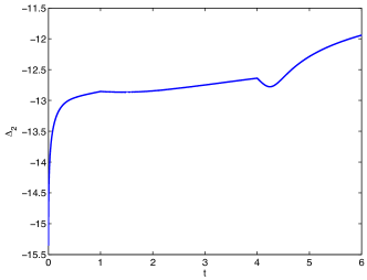
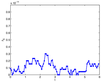
Fig. 1: Time evolution of the $L_{2}$ norm of the difference between the numerical and the exact solutions $\Delta_{2}$ for the isolated soliton on the left, and of the numerically computed energy $\Delta_{E}$ on the right

The numerical solution is shown at several times in Fig. 2, it travels with constant speed $\sqrt{2}$, and the Fourier coefficients are shown in Fig. 3 at $t=t_{max}=6$. For all models the Fourier coefficients decay to machine precision ($\sim 10^{-14}$), and no modulational instability occurs up to the maximal time of computation. This shows that our codes are able to propagate the exact solution even for the unstable case (2d elliptic NLS). It also allows to use the quantity $\Delta_{E}$ as an indicator for the numerical accuracy as in [29, 30, 31].

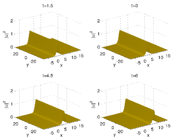
Fig. 2: Isolated soliton at several times in $(2+1)$-dimensional models

Fig. 3: Fourier coefficients of the numerically computed isolated soliton (5) with parameters $(\lambda,v,\phi_{0},x_{0})=(1,\sqrt{2},0,0)$ at $t=t_{max}=6$.

On such travelling waves, it is expected and actually found that the ASM (16) produces a constant value for $\delta(t)$, see Fig. 4, where we find that $\delta(t)\sim 1.57$ for all times studied, and the Fourier coefficients show an exponential decay so that one gets $B=0$ for all times studied.

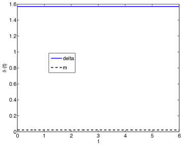
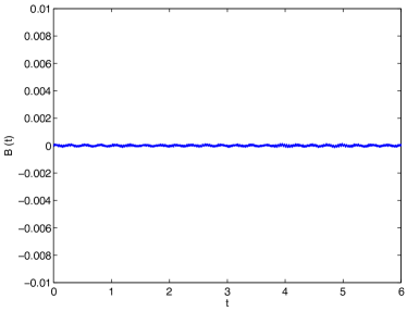
Fig. 4: Time evolution of the fitting parameters in (16), $\delta$ on the left and B on the right, for the numerically computed isolated soliton (5) with parameters $(\lambda,v,\phi_{0},x_{0})=(1,\sqrt{2},0,0)$. The fitting is done for $10<k_{x}<2max(k_{x})/3$

In this section, we explained the numerical tools used for the numerical study of the transverse (in)-stability of the isolated soliton of the 1d cubic NLS equation in higher dimensional models. We showed that we can numerically efficiently reproduce the exact solution under the flow of all models considered, typically with spectral accuracy. In the next section, we investigate the transverse stability of the isolated soliton under localized perturbations.

4 Localized Perturbations (by a Gaussian function)

In this section we consider perturbations of the isolated soliton with a Gaussian function, and investigate its transverse (in-)stability under the flow of different higher models. More precisely, it is known that the isolated soliton (5) is nonlinearly unstable under the 2d cubic NLS flow [42]. Such kind of analytical results however do not provide any idea about the qualitative behavior of the perturbed solutions. The cubic 2d NLS equation (NLS⁺) being in addition known to allow blow up phenomena, it is also interesting to simulate such situations in this context. The similitudes between NLS⁺ and DS⁺⁺ allow one to expect the same kind of results for both models. We will see that in both cases, the instability of the isolated soliton occurs via a $L_{\infty}$-blow up of the solution in one spatial point. On the other hand, we perform a similar study for the hyperbolic variants, NLS^- and DS II. Here theoretical analysis as in [42] no longer hold, and we will see that (5) appears to be unstable in NLS^- and ’orbitally’ stable for DS II.

We thus propagate initial data of the form

$$u(x,y,0)=u_{I}(x,y,0)+A\exp(-(x-x_{1})^{2}-(y-y_{1})^{2}),$$ (19)

where $u_{I}$ denotes the isolated solution (5), $A\in\mathbb{R}$ and $(x_{1},y_{1})\in[-L_{x}\pi,L_{x}\pi]\times[-L_{y}\pi,L_{y}\pi]$.

4.1 Elliptic NLS equations

In this section, the computations are carried out with $2^{13}\times 2^{13}$ points for $x\times y\in[-15\pi,15\pi]\times[-15\pi,15\pi]$.

We first consider an initial data of the form (19) with $(x_{1},y_{1})=(0,0)$ for the NLS⁺ equation. For $A=0.1$, we chose the time step as $\Delta_{t}=6*10^{-4}$, and observe that, as expected, the perturbed soliton under the 2d cubic NLS flow is unstable. We show in Fig.5 the numerical solution at several times, it appears that the solution will blow up at $t^{*}=5.148$, where $\delta$ in (16) vanishes, see Fig. 7.

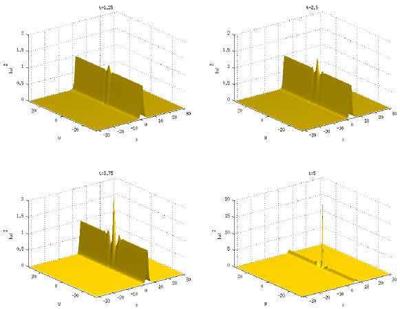
Fig. 5: Solution of the 2d cubic NLS⁺ equation at several times for an initial data of the form (19) with $A=0.1$ and $(x_{1},y_{1})=(0,0)$.

The Fourier coefficients of the solution at $t=5$ still decrease to machine precision $\sim 10^{-15}$, see Fig. 6. That means that the system is still well resolved until $t=5$, just before the blow up time.

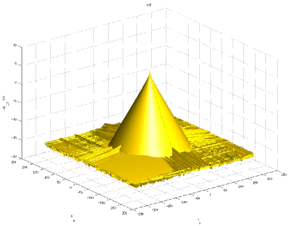
Fig. 6: Fourier coefficients of the solution shown in Fig. 5 at $t=5$.

At $t=t^{*}=5.148$, $\|u\|_{\infty}$ reaches a value of $\sim 50$, and $\|u_{x}\|_{\infty}\sim 1819$. The fitting error $p$ is of the order of $\sim 0.05$, indicating that the fitting is reliable, and that the blow up time is recovered with sufficient accuracy. It is already clear from the pictures, that the blow up appears in only one spatial point, the location of the latter can be also identified as explained in section 3.2, here one finds $\alpha(t^{*})=7.2162$. The value of the numerically computed energy at $t=t^{*}$ is $\Delta_{E}\sim 10^{-15}$, indicating that the system is still well resolved, and that the asymptotic Fourier analysis provides also a determination of the blow up time before the ’typical’ crash of the numerical code.

The situation is similar for other values of $A>0$, the more we add energy to the initial data, the earlier is the blow up time. We show in Fig. 7 the time evolution of $\|u^{A}\|_{\infty}$ for several values of $A$, $u^{A}$ denoting the solution to the NLS⁺ equation for an initial data of the form (19), with $(x_{1},y_{1})=(0,0)$, and the time evolution of the corresponding fitting parameter $\delta(t)$ in (16).

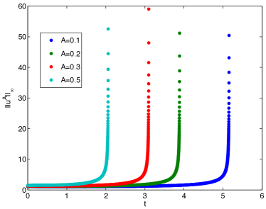
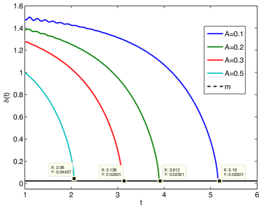
Fig. 7: Time evolution of the $L_{\infty}$-norm of the solutions $u^{A}$ to the NLS⁺ equation for an initial data of the form (19) with $(x_{1},y_{1})=(0,0)$ for several values of $A$ on the left, and the corresponding fitting parameter $\delta(t)$ in (16) on the right.

The transverse instability of the isolated soliton (5) in the 2d cubic NLS⁺ equation for localized perturbations thus appears to be characterized by the appearance of a $L_{\infty}$ blow up of the solution at one spatial point.

One thus expects that a similar study for perturbations of the isolated soliton under the flow of the DS⁺⁺ system leads to similar results. It has been however not yet proved, and the theory in [41] does not seem to hold in this case due to the coupled mean field in the nonlinear part of the equation. We thus consider now an initial data of the form (19) with $(x_{1},y_{1})=(0,0)$ for the DS⁺⁺ system.
For $A=0.1$, and $\Delta_{t}=5*10^{-4}$, we show the solution of the DS⁺⁺ system at several times in Fig. 8.

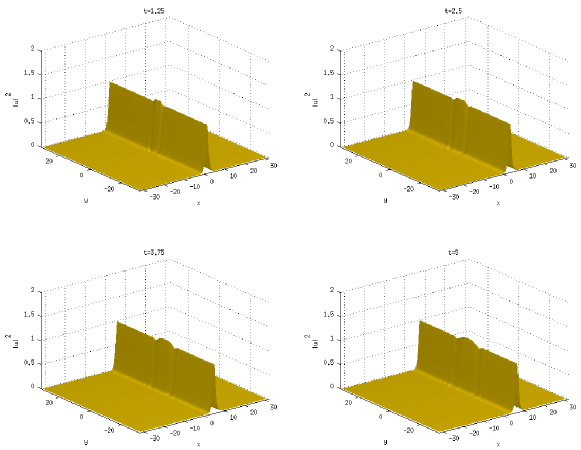
Fig. 8: Solution of the DS⁺⁺ system at several times for an initial data of the form (19) with $(x_{1},y_{1})=(0,0)$ with $A=0.1$.

The situation differs from the previous study, due to the contribution of the coupled mean field $\Phi$ in the system (9). The localized perturbation is somehow more spread in the $y$-direction. The time evolution of the $L_{\infty}$-norm of $u$ is shown in Fig. 9, where we observe that after a rapid decrease, it increases again. The Fourier coefficients reach machine precision all along the computation, see for example the situation at $t=5$ in Fig. 9, as well as the numerically computed energy $\Delta_{E}$ typically used as an indicator of numerical accuracy, (one has $\Delta_{E}\sim 10^{-15}$ at $t=5$).

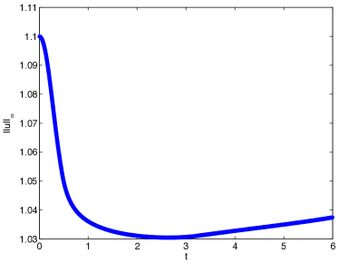
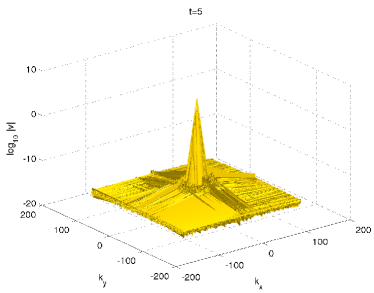
Fig. 9: Time evolution of the $L_{\infty}$-norm of the solution shown in Fig. 8 on the left, and its Fourier coefficients at $t_{max}=5$ on the right.

If the code is run for longer time, one finds that the numerical solution will actually blow up, as for the NLS⁺ case. We show in Fig. 10 the solution at later times.

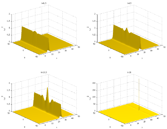
Fig. 10: Solution of the DS⁺⁺ system at several times for an initial data of the form (19) with $(x_{1},y_{1})=(0,0)$ and $A=0.1$.

As before, we perform the fitting of the Fourier coefficients of $u$ on the interval $10<k_{x}<2max(k_{x})/3$, following the well known de-aliasing rule. The vanishing of $\delta(t)$ occurs at $t=t^{*}=26.4$ indicating that a singularity occurs at this time. The value of the fitting parameter $B$ at $t^{*}$ is of the order of $\sim 0.6$, which allows to conjecture a blow up of the solution in the $L_{\infty}$-norm, which can also be inferred from the value of the $L_{\infty}$-norm of $u$ at this time, $\|u\|_{\infty}\sim 40$. The fitting error reaches a value of $p=0.3$. This indicates that the fitting is reliable, one typically expect an error not higher than $0.5$ especially for blow up situations we are looking at, see also [33]. The determination of the location of the singularity as in (17) yields $\alpha(t^{*})=36.79$, and $\Delta_{E}\sim{10^{-14}}$ at $t=t^{*}$.

The situation is similar for higher values of $A$, and we show in Fig. 11 the $L_{\infty}$-norm of the solutions $u^{A}$ to the DS⁺⁺ equation for an initial data of the form (19) with $(x_{1},y_{1})=(0,0)$ for several values of $A$ on the right, and the time evolution of the corresponding $\delta(t)$ in (16) on the left.

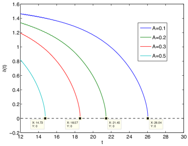
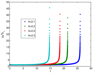
Fig. 11: Time evolution of the fitting parameter $\delta(t)$ on the left and of the $L_{\infty}$-norm of the solutions $u^{A}$ (on the right) to the DS⁺⁺ equation for an initial data of the form (19) and $(x_{1},y_{1})=(0,0)$ for several values of $A$.

The blow up times are also reported in Table 1 for the NLS⁺ and DS⁺⁺ equations.

$A$	$0.1$	$0.2$	$0.3$	$0.5$
$t^{*}_{NLS^{+}}$	$5.16$	$3.89$	$3.10$	$2.06$
$t^{*}_{DS^{++}}$	$26.04$	$21.45$	$18.57$	$14.73$

Table 1: Blow up times of the solutions of the NLS⁺ ($t^{*}_{NLS^{+}}$) and of the DS⁺⁺ ($t^{*}_{DS^{++}}$) equation for an initial data of the form (19) with $(x_{1},y_{1})=(0,0)$ for several values of $A$

In this section, we illustrated numerically the instability of the isolated soliton (5) under the flow of the 2d elliptic NLS equation, and observed that this instability is characterized by the appearance of a blow up in one spatial point. Moreover, we performed the same study for the DS⁺⁺ system. Due to its elliptic character and the parameter chosen, a similar behavior was expected and actually observed. Localized perturbations to the isolated soliton lead also to a blow up here, at a later time though, because of the contribution of the the coupled elliptic equation for the mean field $\Phi$, which tends to extend the perturbation along the $y$-axis. As expected, the isolated soliton is thus found to be nonlinearly unstable under the flow of the DS⁺⁺ system.

4.2 Hyperbolic NLS Equations

In this section, we investigate the transverse (in)-stability of the isolated soliton (5) under the flow of hyperbolic NLS equations by studying again Gaussian perturbations of the form (19). We first perform simulations for the 2d hyperbolic cubic NLS (NLS^-), and then for the focusing DS II equation. It is found that we the perturbed isolated soliton is unstable under the flow of the 2d hyperbolic NLS equation, and that this instability occurs via dispersion, and it appears to be orbitrarily stable under the flow of DS II for Gaussian perturbations of the form 19 with $0<A<1$.

For $A=0.1$, we choose the time step as $\Delta_{t}=2*10^{-3}$, and observe that, as expected, the perturbed soliton under the flow of NLS^- flow is unstable. Recall that in this context only linear analysis is available in the literature. We show in Fig.12 the numerical solution at several times, it appears that the solution becomes chaotic and totally looses the shape and typical features of the original soliton.

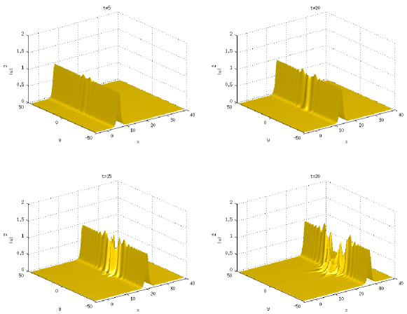
Fig. 12: Solution of the 2d cubic NLS^- equation at several times for an initial data of the form (19) with $A=0.1$ and $(x_{1},y_{1})=(0,0)$.

The situation is even clearer in Fig. 13, where we show the corresponding contour plots of the solution.

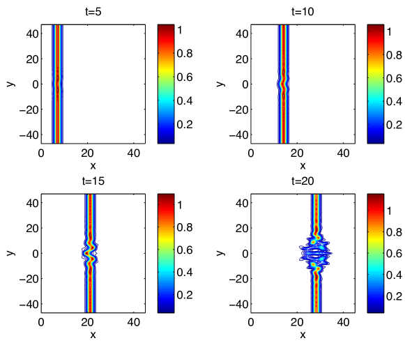
Fig. 13: Contour plots of the solution shown in Fig . 12

It seems the original soliton will totally disperse for longer times. In fact, as we can infer from Fig. 14, where we show the contour plot of the difference between the numerical solution and the original soliton, the perturbation travels at the same velocity as the isolated soliton and simply disperses away. The dispersion of the perturbation yields then the dispersion of the full numerical solution.

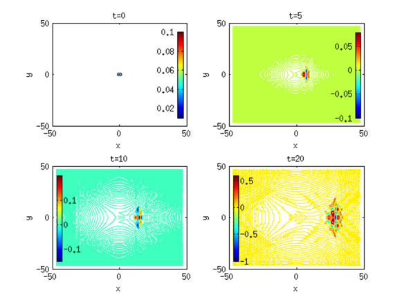
Fig. 14: Contour plots of the difference between the numerical solution shown in Fig. 12 and the original soliton at several times

We ensure that the system is well resolved by checking the good decay of the Fourier coefficients all along the computation, they decrease to machine precision ($10^{-15}$) at all times considered. We show in Fig. 15 the Fourier coefficients of the solution at several times plotted on the $k_{x}$-axis on the left, and plotted in both spatial directions at $t=20$ on the right.

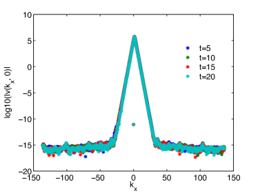
Fig. 15: Fourier coefficients of the solution shown in Fig. 12 at several times plotted on the $k_{x}$-axis on the left, and at $t=20$ on the right (plotted in both directions)

The same behavior was observed for higher values of $A$. The instability of the isolated soliton thus appears to occur though/via the dispersion of the solution as $t$ tends to infinity.

We now perform the same study for the DS II equation. We show the numerical solution at several times in Fig .16.

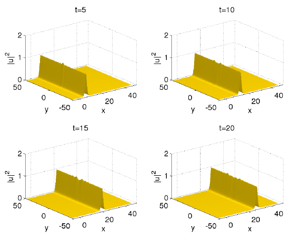
Fig. 16: Solution to the focusing DS II equation for an initial condition of the form (19), with $A=0.1$ and $(x_{1},y_{1})=(0,0)$, at several times.

In this case the perturbation seems to be somehow distributed along the isolated soliton, in the $y$-direction. The $L_{\infty}$-norm of $u$ decreases as $t\to\infty$, see Fig. 17, where we show also the situation for other values of $0<A<1$ until $t=5$. It seems it will stabilise for later times.

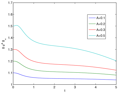
Fig. 17: Time evolution of the $L_{\infty}$-norm of the solutions $u^{A}$ to the focusing DS II equation for an initial condition of the form (19) with $(x_{1},y_{1})=(0,0)$, for several values of $A$.

The fitting of the Fourier coefficients appears to be reliable, with a fitting error of the order of $p\sim 0.1$ all along the computation. One finds that $\delta(t)$ is almost constant $\delta(t)\sim 1.5$, for all times $t\leq 20$ studied, indicating the regularity of the solution.

The numerical accuracy is ensured by the decay to machine precision ($\sim 10^{-15}$) of the Fourier coefficients, , see Fig. 18, and the conservation of the numerically computed energy, $\Delta_{E}$, which reaches the same order as the latter ($\Delta_{E}\sim 10^{-15}$) all along the computation.

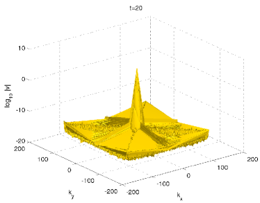
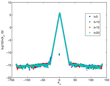
Fig. 18: Fourier coefficients of the solution to the focusing DS II equation for an initial condition of the form (19), with $A=0.1$ and $(x_{1},y_{1})=(0,0)$, at $t=20$ on the left, and at several times (plotted on the $k_{x}$-axis on the right).

In this case, the solution preserves the shape of the original soliton, see Fig. 19 for the contour plots of the solution shown in Fig. 16,

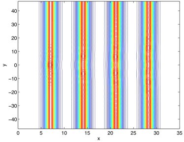
Fig. 19: Contour plots of the solution shown in Fig. 16 at several times, from the left to the right: $t=5,10,15,20$.

and the perturbation itself takes the form of a soliton, see Fig. 20.

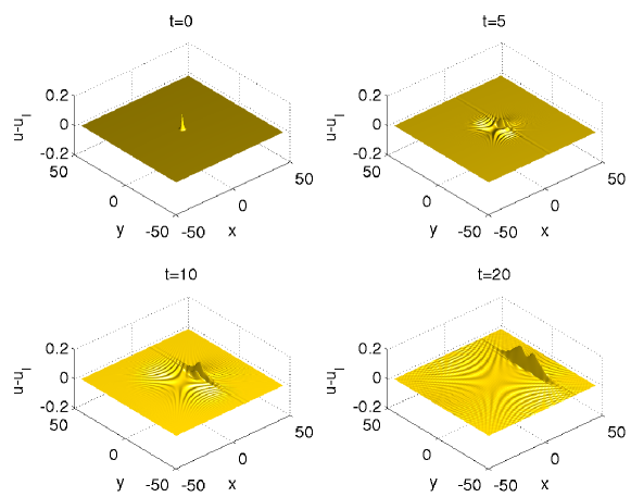
Fig. 20: Difference between the solution of the DS II equation for an initial data of the form (19) with $(x_{1},y_{1})=(0,0)$ and the original soliton $u_{I}$ at several times.

It is clearer when the code is run for longer times on a bigger domain of computation. One finds that the initially localized perturbation is indeed spread in the $y$-direction, and take finally itself the shape of a soliton, see see Fig. 21, where we show the contour plot of the difference between the numerical solution and the original soliton at several times.

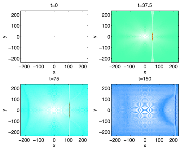
Fig. 21: Contour plots of the difference between the solution of the DS II equation for an initial data of the form (19) with $(x_{1},y_{1})=(0,0)$ and the original soliton $u_{I}$ at several times

The solution asymptotically preserves the soliton’s shape, see Fig. 22 for the situation at $t=100$ and the contour plot in the same picture.

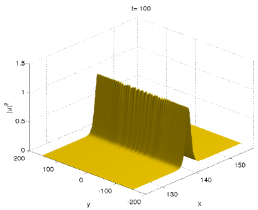
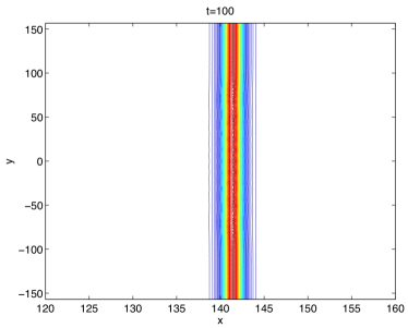
Fig. 22: Solution of the DS II equation for an initial data of the form (19) with $A=0.1$, at $t=100$ on the left, and contour plot on the right.

It appears that the perturbation travels with the soliton and leads also to oscillations around it. Notice that the speed of the soliton is not affected, indicating that no new soliton is formed here. The propagation of the perturbation is still present for large times, so it is difficult to decide if they will finally disappear.

The situation is similar for all values of $A$ studied, and we show the $L_{\infty}$-norm of $u^{A}$ in Fig. 23, it decreases before stabilizing for longer times in all cases.

Fig. 23: Time evolution of the $L_{\infty}$-norm of the solutions $u^{A}$ to the focusing DS II equation for an initial condition of the form (19) with $(x_{1},y_{1})=(0,0)$, for several values of $A$, until $t=150$.

Until now we considered perturbations centered as the same location as the original soliton, i.e., $x_{0}=0$ in (5) and $u_{pert}=\exp(-(x-x_{1})^{2}-(y-y_{1})^{2})$ with $(x_{1},y_{1})=(0,0)$. If instead, one considers a de-centered Gaussian perturbation, i.e., either $(x_{1},y_{1})=(a,0)$ or $(x_{1},y_{1})=(a,b)$, with $(a,b)\in[-L_{x}\pi,L_{x}\pi]\times[-L_{y}\pi,L_{y}\pi]$, one observes that the perturbation simply disperses as $t$ goes to infinity, and has no real impact on the soliton behavior.

To illustrate this, we consider an initial data of the form (19), with $(x_{1},y_{1})=(-L_{x}/2,0)$. The computation is carried out with $2^{13}\times 2^{13}$ points for $x\times y\in[-15\pi,15\pi]\times[-15\pi,15\pi]$ and $\Delta_{t}=3*10^{-3}$. We show in Fig. 24 the resulting numerical solution of DS II at several times.

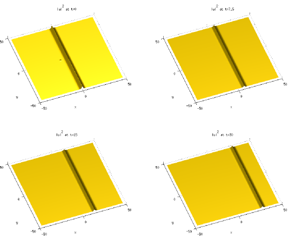
Fig. 24: Solution to the focusing DS II equation for an initial condition of the form (19), with $A=0.1$ and $(x_{1},y_{1})=(-L_{x}/2,0)$, at several times.

The solution travels with the original velocity, and its shape is preserved. The difference between the solution and the original soliton $u_{I}$ are shown in Fig. 25. One can see that the perturbation simply disperses away in the form of tails to infinity.

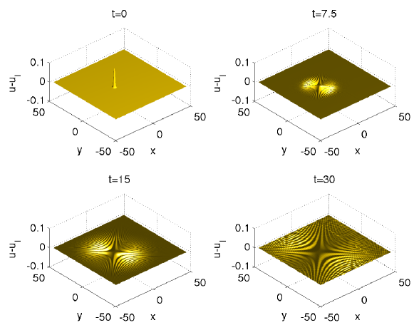
Fig. 25: Difference between the solution of the DS II equation for an initial data of the form (19) with $(x_{1},y_{1})=(L_{x}/2,0)$ and the original soliton $u_{I}$ at several times

It is even clearer in the contour plots shown in Fig. 26.

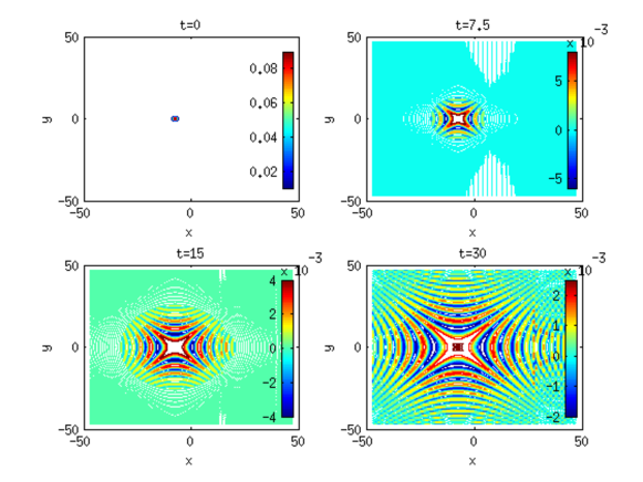
Fig. 26: Contour plots of the solution shown in Fig . 25

The $L_{\infty}$-norm of the solution is shown in Fig. 27 together with the Fourier coefficients at several times. The latter reach machine precision all along the computation, indicating sufficient accuracy, and the $L_{\infty}$-norm of $u$ stays almost constant.

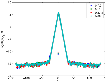
Fig. 27: Time evolution of the $L_{\infty}$-norm of the solution shown in Fig. 24 on the left, and its Fourier coefficients at several times on the right

The soliton appears to be unaffected by the perturbation which appears to smear out in the background of the soliton. The same behavior was observed for initial data of the form (19) with $y_{1}$ non equal to $0$.

For localized perturbations, we found that the perturbed isolated soliton is unstable under the flow of the 2d hyperbolic NLS equation, and that this instability occurs via dispersion. The study of (5) under the flow of DS II however indicates that numerical solutions issued from Gaussian perturbations travel with unchanged speed, and have a profile very close to the original one, in particular the $L_{\infty}$-norm of $u$ becomes constant as $t\to\infty$. The perturbed solution recovers the features of a soliton for all cases studied there, including de-centered Gaussian perturbations. The isolated soliton appears in this sense orbitrarily stable under Gaussian perturbations of the form 19 with $0<A<1$. This a noticeable difference with the results for the 2d (both hyperbolic and elliptic) NLS equations, in which the isolated soliton is unstable.

5 Periodic deformations

We now consider periodic deformations of the isolated soliton (5). More precisely, we consider initial data of the form

$$u(x,y,0)=u_{I}(x,0)(1+\epsilon\cos(\gamma y/L_{y})),\epsilon\ll 1,\gamma\in\mathbb{R}$$ (20)

for the four models we are considering in this paper. The analytical results in [42] provide also here the instability of (5) for the 2d elliptic NLS equation under this kind of perturbations. We will see that in this case, this instability occurs via a blow up in multiple spatial points. For the NLS equation, such behavior has been studied by Merle [16], and we find in addition that such phenomena occur also in the case of DS⁺⁺, for which however no theoretical study is available in this context. The isolated soliton (5) appears to be unstable under periodic perturbations of the form (20) for all cases here.

5.1 Elliptic NLS Equations

We first consider an initial data of the form (20) with $\epsilon=0.1$ and $b=2$ for the 2d elliptic NLS equation (NLS⁺). The computations are carried out with $2^{13}\times 2^{13}$ points for $x\times y\in[-15\pi,15\pi]\times[-15\pi,15\pi]$ and $\Delta_{t}=6*10^{-4}$. As in the previous section, we study the asymptotics of the Fourier coefficients all along the computation, and choose the following range of wavenumbers for the fitting, $10<k_{x}<2\max(k_{x})/3$. For the situation here, we found that a multiple blow up occurs at $t^{*}=10.107$, where $\delta$ as in (16) vanishes. We show in Fig. 28 the numerical solution at several times, including $t^{*}$.

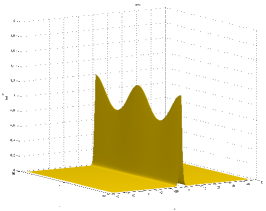
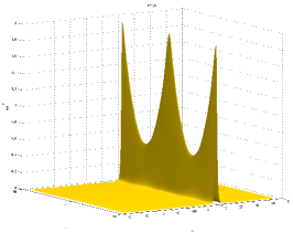
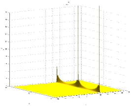
Fig. 28: Solution to NLS⁺ for an initial condition of the form (20), with $\epsilon=0.1$, $b=2$ at several times

The time evolution of $\delta$ as in (16) and of the $L_{\infty}$-norm of $u$ are shown in Fig. 29.

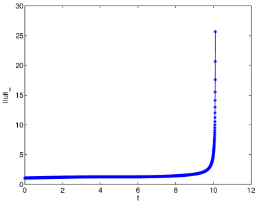
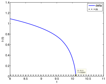
Fig. 29: Time evolution of the $L_{\infty}$-norm of the solution shown in Fig. 28 on the left, and the corresponding fitting parameter $\delta(t)$ in (16) on the right.

At $t^{*}$, $\|u\|_{\infty}\sim 25$. The fitting error is of the order of $p\sim 0.13$ at $t=t^{*}$, and $B$ in 16 reaches a value of $B(t^{*})=0.4852$ indicating clearly a $L_{\infty}$ blow up. Notice that, in this configuration, (multiple blow up points) it was not clear how well the parameter $B$ could reach such value. Some other tests in this context are needed to be able to decide if the asymptotics of the Fourier coefficients can identify or not with such good precision the kind of the singularity via the parameter $B$. Notice that even for one spatial point blow up, the parameter B is not always reliable, as pointed out in [33]. The numerically computed energy is of the order of $\Delta_{E}\sim 10^{-14}$, indicating that the system is well resolved until the singularity formation. In this case, the blow up of the solution occurs in multiple spatial points, located on the same $x$ locations, that we can identify via the formula (17). One finds here that $\alpha(t^{*})=14.2739$. The $y$-locations correspond to the maxima of the solution, i.e. the values of $y$ such that $\sin(\gamma y/L_{y})=0$, i.e., $\gamma y/L_{y}=0\,\,\mbox{modulo}\,\,\pi$. For the example here, we thus get three spatial blow up points. The Fourier coefficients are shown in Fig. 30 at several times.

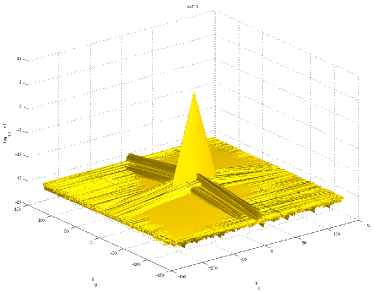
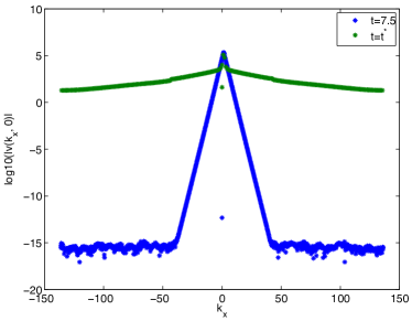
Fig. 30: Fourier coefficients of the solution shown in Fig. 28

If one varies $\gamma$, i.e., the period, one observes that the number of blow up points corresponds to the number of maximum of the solution, for example for $\gamma=4$, one gets 5 blow up space locations, see Fig .31.

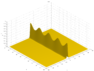
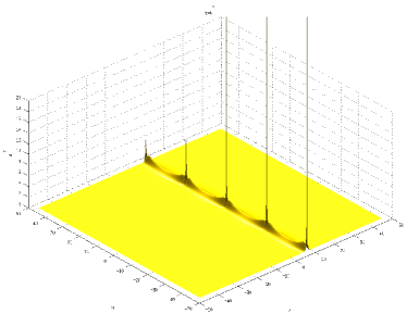
Fig. 31: Solution to NLS⁺ for an initial condition of the form (20), with $\epsilon=0.1$, $b=4$ at several times

In this case, the blow up occurs at $t^{*}=5.871$, where $B=0.5435$ and $p\sim 0.04$, with $\|u\|_{\infty}\sim 32$, $\Delta_{E}\sim 10^{-14}$ and $\alpha(t^{*})=8.2983$.

The same phenomena are observed if one considers an initial data of the form (20) for the DS⁺⁺ equation. We show in Fig. 32 the solution of DS⁺⁺ for an initial data of the form (20) with $\gamma=2$ and $\epsilon=0.1$ at several times.

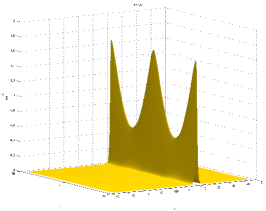
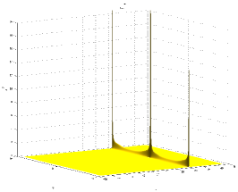
Fig. 32: Solution to DS${}^{+}+$ for an initial condition of the form (20), with $\epsilon=0.1$, $b=2$ at several times

In this case, the vanishing of $\delta$ (as in (16)) occurs at $t^{*}=14.778$, with $\|u\|_{\infty}\sim 35$, see Fig. 33, where we show the time evolution of these two quantities. One finds also $B=0.5036$ and $p\sim 0.3$, $\Delta_{E}\sim 10^{-14}$ and $\alpha(t^{*})=20.8731$. We recover in this case also a value of $B$ in 16 really convincing.

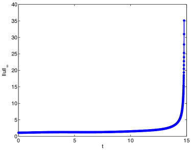
Fig. 33: Time evolution of the $L_{\infty}$-norm of the solution shown in Fig. 32 on the left, and the corresponding fitting parameter $\delta(t)$ in (16) on the right.

The situation here is really similar to the previous case, and we see that the instability of the isolated soliton 5 under periodic perturbations for elliptic models studied there occurs via a multiple blow up point. Recall once again that this instability was known for the NLS⁺ but not yet for DS⁺⁺, and that the features of this instability were up to now not known. The phenomena of multiple blowing-up solutions in DS⁺⁺ has been also not studied (as far as we know), and it would be interesting to see if the theory as by Merle in [16] can be applied there.

5.2 Hyperbolic NLS Equations

We now perform the same study, but for the hyperbolic NLS equations, NLS^- and the DS II equation. The computations are carried out with $2^{13}\times 2^{13}$ points for $x\times y\in[-15\pi,15\pi]\times[-15\pi,15\pi]$ and $\Delta_{t}=2*10^{-3}$.

For the NLS^- equation we consider an initial data of the form (20) with $b=2$ and $\epsilon=0.2$, and show in Fig. 34 the solution at several times.

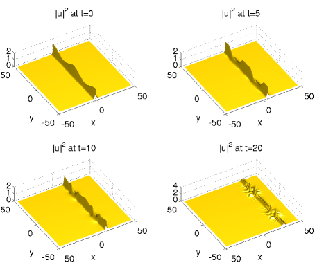
Fig. 34: Solution to NLS^- for an initial condition of the form (20), with $\epsilon=0.2$, $b=2$ at several times

We can see that the solution spreads in the $y$-direction, and tends to recover the initial shape of the soliton, before being decomposed as in the case of localized perturbations studied in the previous section.

The difference between the solution to NLS^- for an initial condition of the form (20), with $\epsilon=0.2$, $b=2$ and the original soliton $u_{I}$ is shown in Fig. 35 at several times.

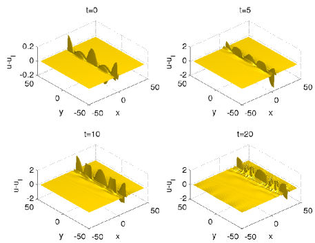
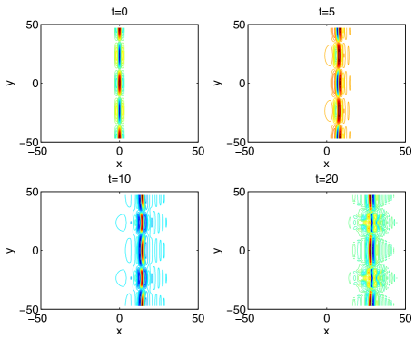
Fig. 35: Difference between the solution to NLS^- for an initial condition of the form (20), with $\epsilon=0.2$, $b=2$ and the original soliton $u_{I}$ at several times

The $L_{\infty}$-norm of the solution is shown in Fig. 36, together with the Fourier coefficients at the maximal time of computation. The latter decrease to machine precision ($10^{-15}$) all along the computation, and $\Delta_{E}\sim 10^{-14}$ at the end of the computation.

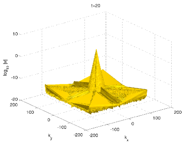
Fig. 36: Time evolution of the $L_{\infty}$-norm of the solution shown in Fig. 34 on the left, and Fourier coefficients of the solution at $t=t_{max}$ on the right

As in the case of localized perturbations, the isolated soliton appears to be unstable under periodic perturbations here in the hyperbolic 2d NLS equation, and this instability occurs via the dispersion of the solution.

For the DS II equation we consider again an initial data of the form (20) with $b=2$ and $\epsilon=0.2$. The solution is shown in Fig. 37 at several times.

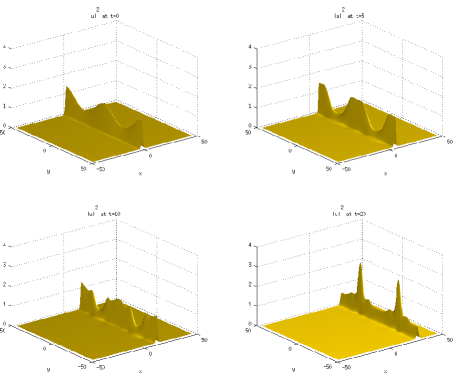
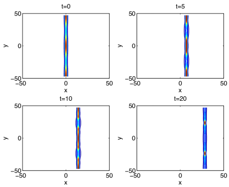
Fig. 37: Solution to DS II for an initial condition of the form (20), with $\epsilon=0.2$, $b=2$ at several times

The difference between the solution to DS II and the original soliton is shown in Fig. 38 at several times. We observe here that the perturbation is also dispersed around the soliton.

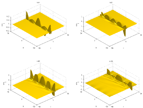
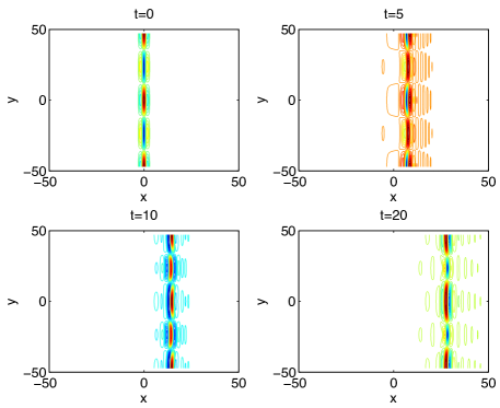
Fig. 38: Difference between the solution to DS II for an initial condition of the form (20), with $\epsilon=0.2$, $b=2$ and the original soliton at several times

The $L_{\infty}$-norm of the solution is shown in Fig. 39, together with the Fourier coefficients of the solution shown in Fig. 37. The latter decrease to machine precision ($10^{-15}$) all along the computation, and $\Delta_{E}\sim 10^{-12}$ at the end of the computation.

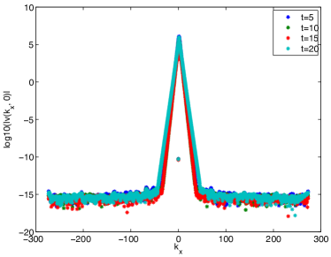
Fig. 39: Time evolution of the $L_{\infty}$-norm of the solution shown in Fig. 37 and Fourier coefficients of the solution shown in Fig. 34 at several times, plotted on the $k_{x}$-axis.

Though it is difficult numerically to determine the long time behavior of the solution shown in Fig. 37, the soliton appears clearly to be unstable under the time evolution of DS II for periodic deformations.

6 Conclusion

In this paper, we addressed numerically the question of the nonlinear transverse stability of the isolated soliton (5) of the 1d cubic NLS equation in higher dimensional models, admissible as transversally perturbed models for it, including elliptic and non-elliptic NLS equations. Whereas for the 2d elliptic cubic NLS, a theory in [42] has been successfully applied to this problem, no such results are known for others models considered in this paper, in particular for hyperbolic NLS equations. In addition, the features of the instability of the isolated soliton (5) under the flow of the 2d elliptic NLS remain unknown from the analysis point of view.

We investigated here these questions numerically, by using efficient numerical schemes for such dispersive PDEs which can develop singularity of blow up type in finite time. The spatial resolution as seen from the Fourier coefficients was always well beyond typical plotting accuracies of the order of $10^{-3}$. For the time integration we used a fourth order time stepping scheme already used in [29, 31, 33] for the study of NLS equations. As argued for instance in [29, 31], the numerically computed energy of the solution gives a valid indicator of the accuracy for sufficient spatial resolution. To ensure the latter, we always presented the Fourier coefficients of the solution. The detection of the singularity formation has been performed thanks to a careful study of the asymptotics of the Fourier coefficients, as used in [46, 32, 33].

We found that the instability of the isolated soliton under the flow of the 2d elliptic NLS equation for localized perturbations occurs via a blow up in the $L_{\infty}$-norm of the solution, in only one spatial point, and for periodic perturbations, this leads to blow up in multiple spatial points. As expected, the same results were observed for the elliptic elliptic DS system, for which, however, neither the instability of (5) have been proved, nor the existence of multiple blowing up solutions.

Another question that we addressed in this paper was the difference between elliptic and hyperbolic variants of NLS in this context. We found that (5) is unstable for both localized and periodic perturbations under the flow of the 2d hyperbolic NLS equation, and that this instability occurs via the dispersion of the solution here.

For the DS II equation, however, we found that the features of the soliton solutions, such as the velocity, shape, and amplitude, remain robust under localized perturbations considered here, and that the perturbation added to the soliton just appears to disperse away in this case. In this sense, the soliton (5) appears to be somehow ’orbitally’ stable under the time evolution of DS II. For periodic perturbations, however, it seems to be unstable.

References

- [1] M.J. Ablowitz and H. Segur. Solitons and the inverse scattering Transform, volume 4 of SIAM Studies in Applied Mathematics. Society for Industrial and Applied Mathematics (SIAM), Philadelphia, Pa., 1981.
- [2] G. Agrawal. Nonlinear fiber optics. Academic Press, San Diego, 2006.
- [3] V.A. Arkadiev, A.K. Pogrebkov, and M.C. Polivanov. Inverse scattering transform method and soliton solutions for the Davey-Stewartson II equation. Physica D, 36:189–196, 1989.
- [4] V. I. Arnol′d, V. V. Kozlov, and A. I. Neĭshtadt. Dynamical Systems. III, volume 3 of Encyclopaedia of Mathematical Sciences. Springer-Verlag, Berlin, 1988. Translated from the Russian by A. Iacob.
- [5] L.Y. Sung A.S. Fokas. On the solvability of the N-wave, the Davey-Stewartson and the Kadomtsev-Petviashmli equation. Inverse Problems, 8:673–708, 1992.
- [6] C. Besse, N.J. Mauser, and H.P. Stimming. Numerical Study of the Davey-Stewartson System. M2AN, 38(6):1035–1054, 2006.
- [7] J. Bourgain. Global solutions of nonlinear Schrödinger equations. American Mathematical Society Colloquium Publications, American Mathematical Society, Providence, RI, 46, 1999.
- [8] Russel E. Caflisch. Singularity formation for complex solutions of the D incompressible Euler equations. Phys. D, 67(1-3):1–18, 1993.
- [9] C. Canuto, M. Y. Hussaini, A. Quarteroni, and T. A. Zang. Spectral methods. Scientific Computation. Springer-Verlag, Berlin, 2006. Fundamentals in single domains.
- [10] G.E. Carrier and M. Krook C.E. Pearson. Functions of a Complex Variable, Theory and Technique. Society for Industrial and Applied Mathematics (SIAM), Philadelphia, PA, 2005.
- [11] T. Cazenave. Semilinear Schrödinger equations. Courant Lecture Notes in Mathematics, New York University Courant Institute of Mathematical Sciences, New York, 10, 2003.
- [12] T. Cazenave and P.L. Lions. Orbital stability of standing waves for some nonlinear Schrödinger equations. Comm. Math. Phys., 85:549–561, 1982.
- [13] C. Conti, S. Trillo, P. Di Trapani, G. Valiulis, A. Piskarskas, O. Jedrkiewicz, , and J. Trull. Nonlinear electromagnetic X waves. Physical Review Letters, 90, 170406:1–4, 2003.
- [14] M. Cross and P. Hohenberg. Pattern formation outside of equilibrium. Rev. Mod. Phys., 65, 1993.
- [15] T.A. Driscoll. A composite Runge-Kutta Method for the spectral Solution of semilinear PDEs. Journal of Computational Physics, 182:357–367, 2002.
- [16] Merle F. Construction of solutions with exactly k blow-up points for the Schrödinger equation with critical nonlinearity. Communications in Mathematical Physics, 129(2):223–240, 1990.
- [17] M. Forest and J. Lee. Geometry and modulation theory for the periodic nonlinear Schrödinger equation. in Oscillation Theory, Computation, and Methods of Compensated Compactness, Minneapolis, MN, 1985. The IMA Volumes in Mathematics and Its Applications, vol. 2, Springer, New York, pages pp. 35–69, 1986.
- [18] M. Frigo and S.G. Johnson. FFTW for version 3.2.2, July 2009.
- [19] U. Frisch, T. Matsumoto, and J. Bec. Singularities of Euler flow? Not out of the blue! J. Statist. Phys., 113(5-6):761–781, 2003. Progress in statistical hydrodynamics (Santa Fe, NM, 2002).
- [20] Rocca G.D., Lombardo M.C., Sammartino M., and Sciacca V. Singularity tracking for Camassa-Holm and Prandtl’s equations. Appl. Numer. Math., 56(8):1108–1122, August 2006.
- [21] J-M Ghidaglia and J-C. Saut. On the initial value problem for the Davey-Stewartson systems. Nonlinearity, 3, 1990.
- [22] J.M. Ghidaglia and J.C. Saut. Nonexistence of travelling wave solutions to nonelliptic nonlinear Schrödinger equations. Journal of Nonlinear Science, 6(2):139–145, 1996.
- [23] M. Grillakis, J. Shatah, and W. Strauss. Stability theory of solitary waves in the presence of symmetry, I. Journal of Functional Analysis, 74(1):160 – 197, 1987.
- [24] M. Grillakis, J. Shatah, and W. Strauss. Stability theory of solitary waves in the presence of symmetry, II. Journal of Functional Analysis, 94(2):308 – 348, 1990.
- [25] W. Gropp, R. Thakur, and E. Lusk. Using MPI-2: Advanced Features of the Message Passing Interface. MIT Press Cambridge, MA, USA, second edition, 1999.
- [26] Berestycki H. and Cazenave T. Instabilit des tats stationaires dans les quations de schr dinger et de klein-gordon non lin aires. C. R. Acad. Sci. Paris S r. I Math., 293(9):489–492, 1981.
- [27] A-K. Kassam and L.N. Trefethen. Fourth-Order Time-Stepping for stiff PDEs. SIAM J. Sci. Comput, 26(4):1214–1233, 2005.
- [28] J. P. Keener and D. W. McLaughlin. Solitons under perturbations. Phys. Rev. A, 16:777–790, Aug 1977.
- [29] C. Klein. Fourth order time-stepping for low dispersion Korteweg-de Vries and nonlinear Schrödinger Equation. Electronic Transactions on Numerical Analysis., 39:116–135, 2008.
- [30] C. Klein, B. Muite, and K. Roidot. Numerical Study of Blowup in the Davey-Stewartson System. DCDS-B, 5:1361–1387, 2013.
- [31] C. Klein and K. Roidot. Fourth order time-stepping for Kadomtsev-Petviashvili and Davey-Stewartson equations. SIAM J. Sci. Comp., 2011.
- [32] C. Klein and K. Roidot. Numerical study of shock formation in the dispersionless Kadomtsev-Petviashvili equation and dispersive regularizations. Physica D: Nonlinear Phenomena, 265:1–25, 2013.
- [33] C. Klein and K. Roidot. Numerical study of the semiclassical limit of the Davey-Stewartson II equations. preprint, 2013.
- [34] Y. Lahini, E. Frumker, Y. Silberberg, S. Droulias, K. Hizanidis, R. Morandotti, and D.N. Christodoulides. Discrete X-wave formation in nonlinear waveguide arrays. Phys. Rev. Lett., 98, 023901:1–4, 2007.
- [35] Pugh M. and Shelley M. Singularity Formation in thin J with Surface Tension. Comm. Pure Appl. Math., 51:733–795, 1998.
- [36] T. Matsumoto, J. Bec, and U. Frisch. The analytic structure of 2D Euler flow at short times. Fluid Dynam. Res., 36(4-6):221–237, 2005.
- [37] M. McConnell, A. S. Fokas, and B. Pelloni. Localised coherent solutions of the DSI and DSII equations—a numerical study. Math. Comput. Simulation, 69(5-6):424–438, 2005.
- [38] F. Merle and P. Raphael. On universality of blow-up profile for critical nonlinear Schrödinger equation. Inventiones Mathematicae, 156:565–672, 2004.
- [39] T. Ozawa. Exact Blow-up Solutions to the Cauchy Problem for the Davey-Stewartson Systems. Proc. Roy. Soc. London Ser. A, 436(1897):345–349, 1992.
- [40] D. E. Pelinovsky. A mysterious threshold for transverse instability of deep-water solitons. Mathematics and Computers in Simulation, 55(4-6):585–594, 2001.
- [41] F. Rousset and N. Tzvetkov. Transverse nonlinear instability of solitary waves for some hamiltonian pde’s. J. Math. Pures Appl, 90:550–590, 2008.
- [42] F. Rousset and N. Tzvetkov. Transverse nonlinear instability for two-dimensional dispersive models. Annales de l’Institut Henri Poincare (C) Non Linear Analysis, 26:2:477–496, 2009.
- [43] Droulias S., Hizanidis K., Meier J., and Christodoulides D. X-waves in nonlinear normally dispersive waveguide arrays. Optics Express, 13(6):1827–1832, 2005.
- [44] D. Senouf, R. Caflisch, and N. Ercolani. Pole dynamics and oscillations for the complex Burgers equation in the small-dispersion limit. Nonlinearity, 9:1671–1702, 1996.
- [45] C. Sulem and P.L. Sulem. The nonlinear Schrödinger equation. Springer, 1999.
- [46] C. Sulem, P.L. Sulem, and H. Frisch. Tracing complex singularities with spectral methods. J. Comp. Phys., 50:138–161, 1983.
- [47] P.-L. Sulem, C. Sulem, and A. Patera. Numerical simulation of singular solutions to the two-dimensional cubic Schrödinger equation. Comm. Pure Appl. Math., 37(6):755–778, 1984.
- [48] L.Y. Sung. Long-time decay of the solutions of the Davey-Stewartson II equations. J. Nonlinear Sci, 5:433–452, 1995.
- [49] P. Di Trapani, G. Valiulis, A. Piskarskas, O. Jedrkiewicz, J. Trull, C. Conti, and S. Trillo. Spontaneously generated X-shaped light bullets. Physical Review Letters, 91, 093904, 2003.
- [50] L.N. Trefethen. Spectral Methods in MATLAB, volume 10 of Software, Environments, and Tools. Society for Industrial and Applied Mathematics (SIAM), Philadelphia, PA, 2000.
- [51] A. Shabat V. Zakharov. Exact theory of two-dimensional self-focusing and one-dimensional self-modulation of waves in nonlinear media. Sov. Phys. JETP, 34:62–69, 1972.
- [52] M.I. Weinstein. Nonlinear Schrödinger equations and sharp interpolation estimates. Comm. Math. Phys., 87:567–576, 1983.
- [53] M.I. Weinstein. Lyapunov stability of ground states of nonlinear dispersive evolution equations. Comm. on Pure and Appl. Math., 39:1:51–67, 1986.
- [54] P.W. White and J.A.C. Weideman. Numerical simulation of solitons and dromions in the Davey-Stewartson system. Math. Comput. Simul., 37(4-5):469–479, December 1994.
- [55] N. Yajima. Stability of envelope soliton. Progress of Theoretical Physics, 52(3):1066–1067, 1974.
- [56] V. E. Zakharov and A. M. Rubenchik. Instability of waveguides and solitons in nonlinear media. Sov. Phys. JETP, 38:494?500, 1974.