Clustering South African households based on their asset status using latent variable models

Abstract

The Agincourt Health and Demographic Surveillance System has since 2001 conducted a biannual household asset survey in order to quantify household socio-economic status (SES) in a rural population living in northeast South Africa. The survey contains binary, ordinal and nominal items. In the absence of income or expenditure data, the SES landscape in the study population is explored and described by clustering the households into homogeneous groups based on their asset status.

A model-based approach to clustering the Agincourt households, based on latent variable models, is proposed. In the case of modeling binary or ordinal items, item response theory models are employed. For nominal survey items, a factor analysis model, similar in nature to a multinomial probit model, is used. Both model types have an underlying latent variable structure—this similarity is exploited and the models are combined to produce a hybrid model capable of handling mixed data types. Further, a mixture of the hybrid models is considered to provide clustering capabilities within the context of mixed binary, ordinal and nominal response data. The proposed model is termed a mixture of factor analyzers for mixed data (MFA-MD).

The MFA-MD model is applied to the survey data to cluster the Agincourt households into homogeneous groups. The model is estimated within the Bayesian paradigm, using a Markov chain Monte Carlo algorithm. Intuitive groupings result, providing insight to the different socio-economic strata within the Agincourt region.

, , , , and

t1Supported by Science Foundation Ireland, Grant number 09/RFP/MTH2367. t2Supported by NIH Grants K01 HD057246, R01 HD054511, R24 AG032112. t3Supported by NIH Grant R01 HD054511 and a Google Faculty Research Award.

1 Introduction

The Agincourt Health and Demographic Surveillance System (HDSS) [Kahn et al. (2007)] continuously monitors the population of 21 villages located in the Bushbuckridge subdistrict of Mpumalanga Province in northeast South Africa. This is a rural population living in what was, during Apartheid, a black “homeland.” The Agincourt HDSS was established in the early 1990s with the purpose of guiding the reorganization of South Africa’s health system. Since then the goals of the HDSS have evolved and now it contributes to evaluation of national policy at population, household and individual levels. Here, the aim is to study the socio-economic status of the households in the Agincourt region.

Asset-based wealth indices are a common way of quantifying wealth in populations for which alternative methods are not feasible [Vyas and Kumaranayake (2006)], such as when income or expenditure data are unavailable. Households in the study area have been surveyed biannually since 2001 to elicit an accounting of assets similar to that used by the Demographic and Health Surveys [Rutstein and Johnson (2004)] to construct a wealth index. The SES landscape is explored by analyzing the most recent survey of assets for each household. The resulting data set contains binary, ordinal and nominal items.

The existence of SES strata or clusters is a well established concept within the sociology literature. Weeden and Grusky (2012), Erikson and Goldthorpe (1992) and Svalfors (2006), for example, expound the idea of SES clusters. Alkema et al. (2008) consider a latent class analysis approach to exploring SES clusters within two of Nairobi’s slum settlements; they posit the existence of 3 and 4 poverty clusters in the two slums, respectively. In a similar vein, here the aim is to examine the SES clustering structure within the set of Agincourt households, based on the asset status survey data. Interest lies in exploring the substantive differences between the SES clusters. Thus, the scientific question of interest can be framed as follows: what are the (dis)similar features of the SES clusters in the set of Agincourt households? This paper aims to answer this question by appropriately clustering the Agincourt households based on asset survey data. The resulting socio-economic group membership information will be used for targeted health care projects and for further surveys of the different socio-economic groups. The SES strata could also serve as valuable inputs to other analyses such as mortality models, and will serve as a key tool in studying poverty dynamics.

To uncover the clustering structure in the Agincourt region, a model is presented here which facilitates clustering of observations in the context of mixed categorical survey data. Latent variable modeling ideas are used, as the observed response is viewed as a categorical manifestation of a latent continuous variable(s). Several models for clustering mixed data have been detailed in the literature. Early work on modeling such data employed the location model [Lawrence and Krzanowski (1996), Hunt and Jorgensen (1999), Willse and Boik (1999)], in which the joint distribution of mixed data is decomposed as the product of the marginal distribution of the categorical variables and the conditional distribution of the continuous variables, given the categorical variables. More recently, Hunt and Jorgensen (2003) reexamined these location models in the presence of missing data. Latent factor models in particular have generated interest for modeling mixed data; Quinn (2004) uses such models in a political science context. Gruhl, Erosheva and Crane (2013) and Murray et al. (2013) use factor analytic models based on a Gaussian copula as a model for mixed data, but not in a clustering context. Everitt (1988), Everitt and Merette (1988) and Muthén and Shedden (1999) provide an early view of clustering mixed data, including the use of latent variable models. Cai et al. (2011), Browne and McNicholas (2012) and Gollini and Murphy (2013) propose clustering models for categorical data based on a latent variable. However, none of the existing suite of clustering methods for mixed categorical data has the capability of modeling the exact nature of the binary, ordinal and nominal variables in the Agincourt survey data, or the desirable feature of modeling all the survey items in a unified framework. The clustering model proposed here presents a unifying latent variable framework by elegantly combining ideas from item response theory (IRT) and from factor analysis models for nominal data.

Item response modeling is an established method for analyzing binary or ordinal response data. First introduced by Thurstone (1925), IRT has its roots in educational testing. Many authors have contributed to the expansion of this theory since then, including Lord (1952), Rasch (1960), Lord and Novick (1968) and Vermunt (2001). Extensions include the graded response model [Samejima (1969)] and the partial credit model [Masters (1982)]. Bayesian approaches to fitting such models are detailed in Johnson and Albert (1999) and Fox (2010). IRT models assume that each observed ordinal response is a manifestation of a latent continuous variable. The observed response will be level $k$, say, if the latent continuous variable lies within a specific interval. Further, IRT models assume that the latent continuous variable is a function of both a respondent specific latent trait variable and item specific parameters.

Modeling nominal response data is typically more complex than modeling binary or ordinal data, as the set of possible responses is unordered. A popular model for nominal choice data is the multinomial probit (MNP) model [Geweke, Keane and Runkle (1994)]. Bayesian approaches to fitting the MNP model have been proposed by Albert and Chib (1993), McCulloch and Rossi (1994), Nobile (1998) and Chib, Greenberg and Chen (1998). The model has also been extended to include multivariate nominal responses by Zhang, Boscardin and Belin (2008). The MNP model treats nominal response data as a manifestation of an underlying multidimensional continuous latent variable, which depends on a respondent’s covariate information and some item specific parameters. Here a factor analysis model for nominal data, similar in nature to the MNP model, is proposed where the observed nominal response is a manifestation of the multidimensional latent variable which is itself modeled as a function of both a respondent’s latent trait variable and some item specific parameters.

The structural similarities between IRT models and the MNP model suggest a hybrid model would be advantageous. Both models have a latent variable structure underlying the observed data which exhibits dependence on item specific parameters. Further, the latent variable in both models has an underlying factor analytic structure through the dependency on the latent trait. This similarity is exploited and the models are combined to produce a hybrid model capable of modeling mixed categorical data types. This hybrid model can be thought of as a factor analysis model for mixed data.

As stated, the motivation here is the need to substantively explore clusters of Agincourt households based on mixed categorical survey data. A model-based approach to clustering is proposed, in that a mixture modeling framework provides the clustering machinery. Specifically, a mixture of the factor analytic models for mixed data is considered to provide clustering capabilities within the context of mixed binary, ordinal and nominal response data. The resulting model is termed the mixture of factor analyzers for mixed data (MFA-MD).

The paper proceeds as follows. Background information about the Agincourt region of South Africa as well as the socio-economic status (SES) survey and resulting data set are introduced in Section 2. IRT models, a model for nominal response data and the amalgamation and extension of these models to a MFA-MD model are considered in Section 3. Section 4 is concerned with Bayesian model estimation and inference. The results from fitting the model to the Agincourt data are presented in Section 5. Finally, discussion of the results and future research areas takes place in Section 6.

2 The Agincourt HDSS data set

The Health and Demographic Survey System (HDSS) covers an area of $420$ km² consisting of 21 villages with a total population of approximately $82\mbox{,}000$ people. The infrastructure in the area is mixed. The roads in and surrounding the study area are in the process of rapidly being upgraded from dirt to tar. The cost of electricity is prohibitively high for many households, though it is available in all villages. A dam has been constructed nearby, but to date there is no piped water to dwellings and sanitation is rudimentary. The soil in the area is generally suited to game farming and there is virtually no commercial farming activity. Most households contain wage earners who purchase maize and other foods which they then supplement with home-grown crops and collected wild foodstuffs.

To explore the SES landscape in Agincourt, data describing assets of households in the Agincourt study area are analyzed. The data consist of the responses of $N=17\mbox{,}617$ households to each of $J=28$ categorical survey items. There are $22$ binary items, $3$ ordinal items and $3$ nominal items. The binary items are asset ownership indicators for the most part. These items record whether or not a household owns a particular asset (e.g., whether or not they own a working car). An example of an ordinal item is the type of toilet the household uses. This follows an ordinal scale from no toilet at all to a modern flush toilet. Finally, the power used for cooking is an example of a nominal item. The household may use electricity, bottled gas or wood, among others. This is an unordered set. A full list of survey items is given in Appendix A. For more information on the Agincourt HDSS and on data collection see www.agincourt.co.za.

Previous analyses of similar mixed categorical asset survey data derive SES strata using principal components analysis. Typically households are grouped into predetermined categories based on the first principal scores, reflecting different SES levels [Vyas and Kumaranayake (2006), Filmer and Pritchett (2001), McKenzie (2005), Gwatkin et al. (2007)]. Filmer and Pritchett (2001), for example, examine the relationship between educational enrollment and wealth in India by constructing an SES asset index based on principal component scores. Percentiles are then used to partition the observations into groups rather than the model-based approach suggested here. In a previous analysis of the Agincourt HDSS survey data, Collinson et al. (2009) construct an asset index for each household. How migration impacts upon this index is then analyzed, rather than the exploration of SES considered here. The routine approach of principal components analysis does not explicitly recognize the data as categorical and, further, the use of such a one-dimensional index will often miss the natural groups that exist with respect to the whole collection of assets and other possible SES variables. The model proposed here aims to alleviate such issues.

3 A mixture of factor analyzers model for mixed data

A mixture of factor analyzers model for mixed data (MFA-MD) is proposed to explore SES clusters of Agincourt households. Each component of the MFA-MD model is a hybrid of an IRT model and a factor analytic model for nominal data. In this section IRT models for ordinal data and a latent variable model for nominal data are introduced, before they are combined and extended to the MFA-MD model.

3.1 Item response theory models for ordinal data

Suppose item $j$(for $j=1,\ldots,J$) is ordinal and the set of possible responses is denoted $\{1,2,\ldots,K_{j}\}$, where $K_{j}$ denotes the number of response levels to item $j$. IRT models assume that, for respondent $i$, a latent Gaussian variable $z_{ij}$ corresponds to each categorical response $y_{ij}$. A Gaussian link function is assumed, though other link functions, such as the logit, are detailed in the IRT literature [Fox (2010), Lord and Novick (1968)].

For each ordinal item $j$ there exists a vector of threshold parameters $\underline{\gamma}_{j}=(\gamma_{j,0},\gamma_{j,1},\ldots,\gamma_{j,K_{j}})$, the elements of which are constrained such that

$$-\infty=\gamma_{j,0}\leq\gamma_{j,1}\leq\cdots\leq\gamma_{j,K_{j}}=\infty.$$

For identifiability reasons [Albert and Chib (1993), Quinn (2004)] $\gamma_{j,1}=0$. The observed ordinal response, $y_{ij}$, for respondent $i$ is a manifestation of the latent variable $z_{ij}$, that is,

$$\mbox{ if }\gamma_{j,k-1}\leq z_{ij}\leq\gamma_{j,k}\qquad\mbox{then }y_{ij}=k.$$ (1)

That is, if the underlying latent continuous variable lies within an interval bounded by the threshold parameters $\gamma_{j,k-1}$ and $\gamma_{j,k}$, then the observed ordinal response is level $k$.

In a standard IRT model, a factor analytic model is then used to model the underlying latent variable $z_{ij}$. It is assumed that the mean of the conditional distribution of $z_{ij}$ depends on a $q$-dimensional, respondent specific, latent variable $\underline{\theta}_{i}$ and on some item specific parameters. The latent variable $\underline{\theta}_{i}$ is sometimes referred to as the latent trait or a respondent’s ability parameter in IRT. Specifically, the underlying latent variable $z_{ij}$ for respondent $i$ and item $j$ is assumed to be distributed as

$$z_{ij}|\underline{\theta}_{i}\sim N\bigl{(}\mu_{j}+\underline{\lambda}_{j}^{T}\underline{\theta}_{i},1\bigr{)}.$$

The parameters $\underline{\lambda}_{j}$ and $\mu_{j}$ are usually termed the item discrimination parameters and the negative item difficulty parameter, respectively. As in Albert and Chib (1993), a probit link function is used so the variance of $z_{ij}$ is $1$.

Under this model, the conditional probability that a response takes a certain ordinal value can be expressed as the difference between two standard Gaussian cumulative distribution functions, that is, $P(y_{ij}=k|\underline{\lambda}_{j},\mu_{j},\underline{\gamma}_{j},\underline{\theta}_{i})$ is

$$\Phi\bigl{[}\gamma_{j,k}-\bigl{(}\mu_{j}+\underline{\lambda}_{j}^{T}\underline{\theta}_{i}\bigr{)}\bigr{]}-\Phi\bigl{[}\gamma_{j,k-1}-\bigl{(}\mu_{j}+\underline{\lambda}_{j}^{T}\underline{\theta}_{i}\bigr{)}\bigr{]}.$$ (2)

Since a binary item can be viewed as an ordinal item with two levels (0 and 1, say), the IRT model can also be used to model binary response data. The threshold parameter for a binary item $j$ is $\underline{\gamma}_{j}=(-\infty,0,\infty)$ and, hence,

$$P(y_{ij}=1|\underline{\lambda}_{j},\mu_{j},\underline{\gamma}_{j},\underline{\theta}_{i})=\Phi\bigl{(}\mu_{j}+\underline{\lambda}_{j}^{T}\underline{\theta}_{i}\bigr{)}.$$

3.2 A factor analytic model for nominal data

Modeling nominal response data is typically more complicated than modeling ordinal data since the set of possible responses is no longer ordered. The set of nominal responses for item $j$ is denoted $\{1,2,\ldots,K_{j}\}$ such that 1 corresponds to the first response choice while $K_{j}$ corresponds to the last response choice, but where no inherent ordering among the choices is assumed.

As detailed in Section 3.1, the IRT model for ordinal data posits a one-dimensional latent variable for each observed ordinal response. In the factor analytic model for nominal data proposed here, a $K_{j}-1$-dimensional latent variable is required for each observed nominal response. That is, the latent variable for observation $i$ corresponding to nominal item $j$ is denoted

$$\underline{z}_{ij}=\bigl{(}z_{ij}^{1},\ldots,z_{ij}^{K_{j}-1}\bigr{)}.$$

The observed nominal response is then assumed to be a manifestation of the values of the elements of $\underline{z}_{ij}$ relative to each other and to a cutoff point, assumed to be $0$. That is,

$$y_{ij}=\cases{1,&\quad$\mbox{if $\max_{k}\bigl{\{}z_{ij}^{k}\bigr{\}}<0$};$\vspace*{2pt}\cr k,&\quad$\mbox{if $z_{ij}^{k-1}=\max_{k}\bigl{\{}z_{ij}^{k}\bigr{\}}$ and $z_{ij}^{k-1}>0$ for $k=2,\ldots,K_{j}$}.$}$$

Similar to the IRT model, the latent vector $\underline{z}_{ij}$ is modeled via a factor analytic model. The mean of the conditional distribution of $\underline{z}_{ij}$ depends on a respondent specific, $q$-dimensional, latent trait, $\underline{\theta}_{i}$, and item specific parameters, that is, $\underline{z}_{ij}|\underline{\theta}_{i}\sim\operatorname{MVN}_{K_{j}-1}(\underline{\mu}{}_{j}+\Lambda_{j}\underline{\theta}_{i},\mathbf{I})$, where $\mathbf{I}$ denotes the identity matrix. The loadings matrix $\Lambda_{j}$ is a $(K_{j}-1)\times q$ matrix, analogous to the item discrimination parameter in the IRT model of Section 3.1; likewise, the mean $\underline{\mu}{}_{j}$ is analogous to the item difficulty parameter in the IRT model.

It should be noted that binary data could be regarded as either ordinal or nominal. The model proposed here is equivalent to the model proposed in Section 3.1 when $K_{j}=2$.

3.3 A factor analysis model for mixed data

It is clear that the IRT model for ordinal data (Section 3.1) and the factor analytic model for nominal data (Section 3.2) are similar in structure. Both model the observed data as a manifestation of an underlying latent variable, which is itself modeled using a factor analytic structure. This similarity is exploited to obtain a hybrid factor analysis model for mixed binary, ordinal and nominal data.

Suppose $Y$, an $N\times J$ matrix of mixed data, denotes the data from $N$ respondents to $J$ survey items. Let $O$ denote the number of binary items plus the number of ordinal items, leaving $J-O$ nominal items. Without loss of generality, suppose that the binary and ordinal items are in the first $O$ columns of $Y$ while the nominal items are in the remaining columns.

The binary and ordinal items are modeled using an IRT model and the nominal items using the factor analytic model for nominal data. Therefore, for each respondent $i$ there are $O$ latent continuous variables corresponding to the ordinal items and $J-O$ latent continuous vectors corresponding to the nominal items. The latent variables and latent vectors for respondent $i$ are collected together in a single $D$-dimensional vector $\underline{z}_{i}$, where $D=O+\sum_{j=O+1}^{J}(K_{j}-1)$. That is, underlying respondent $i$’s set of $J$ binary, ordinal and nominal responses lies the latent vector

$$\underline{z}_{i}=\bigl{(}z_{i1},\ldots,z_{iO},\ldots,z_{iJ}^{1},\ldots,z_{iJ}^{K_{J}-1}\bigr{)}.$$

This latent vector is then modeled using a factor analytic structure:

$$\underline{z}_{i}|\underline{\theta}_{i}\sim\operatorname{MVN}_{D}(\underline{\mu}+\Lambda\underline{\theta}_{i},\mathbf{I}).$$ (3)

The $D\times q$-dimensional matrix $\Lambda$ is termed the loadings matrix and $\underline{\mu}$ is the $D$-dimensional mean vector. Combining the IRT and factor analytic models in this way facilitates the modeling of binary, ordinal and nominal response data in an elegant and unifying latent variable framework.

The model in (3) provides a parsimonious factor analysis model for the high-dimensional latent vector $\underline{z}_{i}$ which underlies the observed mixed data. As in any model which relies on a factor analytic structure, the loadings matrix details the relationship between the low-dimensional latent trait $\underline{\theta}_{i}$ and the high-dimensional latent vector $\underline{z}_{i}$. Marginally, the latent vector is distributed as

$$\underline{z}_{i}\sim\operatorname{MVN}_{D}\bigl{(}\underline{\mu},\Lambda\Lambda^{T}+\mathbf{I}\bigr{)},$$

resulting in a parsimonious covariance structure for $\underline{z}_{i}$.

3.4 A mixture of factor analyzers model for mixed data

To facilitate clustering when the observed data are mixed categorical variables, a mixture modeling framework can be imposed on the hybrid model defined in Section 3.3. The resulting model is termed the mixture of factor analyzers model for mixed data. In the MFA-MD model, the clustering is deemed to occur at the latent variable level, that is, under the MFA-MD model the distribution of the latent data $\underline{z}_{i}$ is modeled as a mixture of $G$ Gaussian densities

$$f(\underline{z}_{i})=\sum_{g=1}^{G}\pi_{g}\operatorname{MVN}_{D}\bigl{(}\underline{\mu}{}_{g},\Lambda_{g}\Lambda_{g}^{T}+\mathbf{I}_{D}\bigr{)}.$$ (4)

The probability of belonging to cluster $g$ is denoted by $\pi_{g}$, where $\sum_{g=1}^{G}\pi_{g}=1$ and $\pi_{g}>0\ \forall g$. The mean and loading parameters are cluster specific.

As is standard in a model-based approach to clustering [Fraley and Raftery (1998), Celeux, Hurn and Robert (2000)], a latent indicator variable, $\underline{\ell}_{i}=(\ell_{i1},\ldots,\ell_{iG})$, is introduced for each respondent $i$. This binary vector indicates the cluster to which individual $i$ belongs, that is, $l_{ig}=1$ if $i$ belongs to cluster $g$; all other entries in the vector are $0$. Under the model in (4), the augmented likelihood function for the $N$ respondents is then given by

$$\mathcal{L}(\underline{\pi},\tilde{\Lambda},\Gamma,Z,\Theta,L|Y)$$

$$\qquad=\prod_{i=1}^{N}\prod_{g=1}^{G}\Biggl{\{}\pi_{g}\Biggl{[}\prod_{j=1}^{O}\prod_{k=1}^{K_{j}}N\bigl{(}z_{ij}|\tilde{\underline{\lambda}}_{gj}^{T}\tilde{\underline{\theta}}_{i},1\bigr{)}^{\mathbb{I}\{\gamma_{j,k-1}<z_{ij}<\gamma_{j,k}|y_{ij}\}}\Biggr{]}$$ (5)

$$\hskip 36.0pt\qquad\quad{}\times\Biggl{[}\prod_{j=O+1}^{J}\prod_{k=2}^{K_{j}}\prod_{s=1}^{3}N\bigl{(}z_{ij}^{k-1}|\tilde{\underline{\lambda}}{}_{gj}^{k-1^{T}}\tilde{\underline{\theta}}_{i},1\bigr{)}^{\mathbb{I}(\mathrm{case}\ s|y_{ij})}\Biggr{]}\Biggr{\}}^{\ell_{ig}},$$

where $\tilde{\underline{\theta}}_{i}=(1,\theta_{i1},\ldots,\theta_{iq})^{T}$ and $\tilde{\Lambda}_{g}$ is the matrix resulting from the combination of $\underline{\mu}{}_{g}$ and $\Lambda_{g}$ so that the first column of $\tilde{\Lambda}_{g}$ is $\underline{\mu}{}_{g}$. Thus, the $d$th row of $\tilde{\Lambda}_{g}$ is $\tilde{\underline{\lambda}}_{gd}=(\mu_{gd},\lambda_{gd1},\ldots,\lambda_{gdq})$.

The likelihood function in (3.4) depends on the observed responses $Y$ through the indicator functions. In the ordinal part of the model, the observed $y_{ij}$ restricts the interval in which $z_{ij}$ lies, as detailed in (1). In the nominal part of the model, $z_{ij}^{k-1}$ is restricted in one of three ways, depending on the observed $y_{ij}$. The three cases $\mathbb{I}(\mathrm{case}\ s|y_{ij})$ for $s=1,2,3$ are defined as follows:

• $\mathbb{I}(\mathrm{case}\ 1|y_{ij})=1$ if $y_{ij}=1$, that is, $\max_{k}\{z_{ij}^{k}\}<0$.

• $\mathbb{I}(\mathrm{case}\ 2|y_{ij})=1$ if $y_{ij}=k$, that is, $z_{ij}^{k-1}=\max_{k}\{z_{ij}^{k}\}$ and $z_{ij}^{k-1}>0$.

• $\mathbb{I}(\mathrm{case}\ 3|y_{ij})=1$ if $y_{ij}\neq 1\land y_{ij}\neq k$, that is, $z_{ij}^{k-1}<\max_{k}\{z_{ij}^{k}\}$.

An example of how this latent variable formulation gives rise to particular nominal responses is given in Appendix B.

The MFA-MD model proposed here is related to the mixture of factor analyzers model [Ghahramani and Hinton (1997)] which is appropriate when the observed data are continuous in nature. Fokoue and Titterington (2003) detail a Bayesian treatment of such a model; McNicholas and Murphy (2008) detail a suite of parsimonious mixture of factor analyzer models.

The MFA-MD model developed here provides a novel approach to clustering the mixed data in the Agincourt survey in a unified framework. In particular, the MFA-MD model has two novel features: (i) it has the capability to appropriately model the exact nature of the data in the Agincourt survey, in particular, the nominal data, and (ii) it has the capability of modeling all the survey items in a unified manner.

4 Bayesian model estimation

A Bayesian approach using Markov chain Monte Carlo (MCMC) is utilized for fitting the MFA-MD model to the Agincourt survey data. Interest lies in the cluster membership vectors $L$ and the mixing proportions $\underline{\pi}$, and in the underlying latent variables $Z$, the latent traits $\Theta$, the item parameters $\tilde{\Lambda}_{g}(\forall g=1,\ldots,G$) and the threshold parameters $\Gamma$.

4.1 Prior and posterior distributions

To fit the MFA-MD model in a Bayesian framework, prior distributions are required for all unknown parameters. As in Albert and Chib (1993), a uniform prior is specified for the threshold parameters. Conjugate prior distributions are specified for the other model parameters:

$$p(\tilde{\underline{\lambda}}_{gd})=\operatorname{MVN}_{(q+1)}(\underline{\mu}_{\lambda},\Sigma_{\lambda}),\qquad p(\underline{\pi})=\operatorname{Dirichlet}(\underline{\alpha}).$$

In terms of latent variables, it is assumed the latent traits $\underline{\theta}_{i}$ follow a standard multivariate Gaussian distribution while the latent indicator variables, $\underline{\ell}_{i}$, follow a $\operatorname{Multinomial}(1,\underline{\pi})$ distribution. Further, conditional on membership of cluster $g$, the latent variable $\underline{z}_{i}|l_{ig}=1\sim\operatorname{MVN}_{D}(\underline{\mu}{}_{g},\Lambda_{g}\Lambda_{g}^{T}+\mathbf{I})$. Combining these latent variable distributions and prior distributions with the likelihood function specified in (3.4) results in the joint posterior distribution, from which samples of the model parameters and latent variables are drawn using a MCMC sampling scheme.

4.2 Estimation via a Markov chain Monte Carlo sampling scheme

As the marginal distributions of the model parameters cannot be obtained analytically, a MCMC sampling scheme is employed. All parameters and latent variables are sampled using Gibbs sampling, with the exception of the threshold parameters $\Gamma$, which are sampled using a Metropolis–Hastings step.

The full conditional distributions for the latent variables and model parameters are detailed below; full derivations are given in McParland et al. (2014a):

• Allocation vectors. For $i=1,\ldots,N$: $\underline{\ell_{i}}|\cdots\sim\operatorname{Multinomial}(\underline{p})$, where $\underline{p}$ is defined in McParland et al. (2014a).

• Latent traits. For $i=1,\ldots,N$: $\underline{\theta}_{i}|\cdots\sim\operatorname{MVN}_{q}\{[\Lambda_{g}^{T}\Lambda_{g}+\mathbf{I}]^{-1}[\Lambda_{g}^{T}(\underline{z}_{i}-\underline{\mu}{}_{g})],\break[\Lambda_{g}^{T}\Lambda_{g}+\mathbf{I}]^{-1}\}$.

• Mixing proportions: $\underline{\pi}|\cdots\sim\operatorname{Dirichlet}(n_{1}+\alpha_{1},\ldots,n_{g}+\alpha_{G})$ where $n_{g}=\sum_{i=1}^{N}\ell_{ig}$.

• Item parameters. For $g=1,\ldots,G$ and $d=1,\ldots,D$: $\tilde{\underline{\lambda}}_{gd}|\cdots\sim\break\operatorname{MVN}_{(q+1)}\{[\Sigma_{\lambda}^{-1}+\tilde{\Theta}_{g}^{T}\tilde{\Theta}_{g}]^{-1}[\tilde{\Theta}_{g}^{T}\underline{z}_{gd}+\Sigma_{\lambda}^{-1}\underline{\mu}_{\lambda}],[\Sigma_{\lambda}^{-1}+\tilde{\Theta}_{g}^{T}\tilde{\Theta}_{g}]^{-1}\}$, where$\underline{z}_{gd}=\{z_{id}\}$ for all respondents $i$ in cluster $g$ and $\tilde{\Theta}_{g}$ is a matrix, the rows of which are $\tilde{\underline{\theta}}_{i}$ for members of cluster $g$.

The full conditional distribution for the underlying latent data $Z$ follows a truncated Gaussian distribution. The point(s) of truncation depends on the nature of the corresponding item, the observed response and the values of $Z$ from the previous iteration of the MCMC chain. The distributions are truncated to satisfy the conditions detailed in Section 3. Thus, the latent data $Z$ are updated as follows:

• If item $j$ is ordinal and $y_{ij}=k$, then

  $$z_{ij}|\cdots\sim N^{T}\bigl{(}\tilde{\underline{\lambda}}{}_{gj}^{T}\tilde{\underline{\theta}}_{i},1\bigr{)},$$

  where the distribution is truncated on the interval $(\gamma_{j,k-1},\gamma_{j,k})$.

• If item $j$ is nominal, then

  $$z_{ij}^{k}|\cdots\sim N^{T}\bigl{(}\tilde{\underline{\lambda}}_{gj}^{k^{T}}\tilde{\underline{\theta}}_{i},1\bigr{)},$$

  where $\tilde{\underline{\lambda}}{}_{gj}^{k}$ is the row of $\tilde{\Lambda}_{g}$ corresponding to $z_{ij}^{k}$ and the truncation intervals are defined as follows:

  • [$-$]

  • if $y_{ij}=1$, then $z_{ij}^{k}\in(-\infty,0)$ for $k=1,\ldots,K_{j}-1$.

  • if $y_{ij}=k>1$, then:

    1. $z_{ij}^{k-1}\in(\tau,\infty)$ where $\tau=\max(0,\max_{l\neq k-1}\{z_{ij}^{l}\})$.

    2. for $l=1,\ldots,k-2,k,\ldots,K_{j}-1$ then $z_{ij}^{l}\in(-\infty,z_{ij}^{k-1})$.

Note that, in the case of $y_{ij}=k>1$ above, the values $z_{ij}^{l}$ considered in the evaluation of $\tau$ in step 1 are those from the previous point in the MCMC chain. The value of $z_{ij}^{k-1}$ in step 2 is that sampled in step 1.

As a uniform prior is specified for the threshold parameters, the posterior full conditional distribution of $\underline{\gamma}_{j}$ is also uniform, facilitating the use of a Gibbs sampler. However, if there are large numbers of observations in adjacent response categories, very slow mixing may be observed. Thus, as in Cowles (1996), Fox (2010), Johnson and Albert (1999), a Metropolis–Hastings step is used to sample the threshold parameters; the overall sampling scheme employed is therefore a Metropolis-within-Gibbs sampler.

Briefly, the Metropolis–Hastings step involves proposing candidate values $v_{j,k}$ (for $k=2,\ldots,K_{j}-1$) for $\gamma_{j,k}$ from the Gaussian distribution $\mathrm{N}^{T}(\gamma_{j,k}^{(t-1)},\break\sigma_{\mathrm{MH}}^{2})$ truncated to the interval $(v_{j,k-1},\gamma_{j,k+1}^{(t-1)})$, where $\gamma_{j,k+1}^{(t-1)}$ is the value of $\gamma_{j,k+1}$ sampled at iteration $(t-1)$. The threshold vector $\underline{\gamma}_{j}$ is set equal to the proposed vector, $\underline{v}_{j}$, with probability $\beta=\min(1,R)$, where $R$ is defined in McParland et al. (2014a). The tuning parameter $\sigma_{\mathrm{MH}}^{2}$ is selected to achieve appropriate acceptance rates.

This Metropolis-within-Gibbs sampling scheme is iterated until convergence, after which the samples drawn are from the joint posterior distribution of all the model parameters and latent variables of the MFA-MD model.

4.3 Model identifiability

The MFA-MD model as described is not identifiable. One identifiability aspect of the model concerns the threshold parameters. If a constant is added to the threshold parameters for an ordinal item $j$ and the same constant is added to the corresponding mean parameter(s), the likelihood remains unchanged. Therefore, as outlined in Section 3.1, the second element $\gamma_{j1}$ of the vector of threshold parameters, $\underline{\gamma}_{j}$, is fixed at $0$ for all ordinal items $j$.

The model is also rotationally invariant due to its factor analytic structure. Many approaches to this identifiability issue have been proposed in the literature. A popular solution is that proposed by Geweke and Zhou (1996) where the loadings matrix is constrained such that the first $q$ rows have a lower triangular form and the diagonal elements are positive. This approach is adopted by Quinn (2004) and Fokoue and Titterington (2003), among others. However, this approach enforces an ordering on the variables [Aguilar and West (2000)] which is not appropriate under the MFA-MD model.

Here, the approach to identifying the MFA-MD model is based on that suggested by Hoff, Raftery and Handcock (2002) and Handcock, Raftery and Tantrum (2007) in relation to latent space models for network data. Instead of imposing a particular form on the loadings matrices, the MCMC samples are post-processed using Procrustean methods. Each sampled $\Lambda_{g}$ is rotated and/or reflected to match as closely as possible to a reference loadings matrix. The latent traits, $\underline{\theta}_{i}$, are then subjected to the same transformation. The sample mean of these transformed values is then used to estimate the mean of the posterior distribution.

Conditional on the cluster memberships on convergence of the MCMC chain, a factor analysis model is fitted to the underlying latent data within each cluster. The estimated loadings matrix obtained is used as the reference matrix for each cluster. Only the saved MCMC samples need to be subjected to this transformation, which is done post hoc and is computationally cheap.

5 Results: Fitting the MFA-MD model to the Agincourt data

In order to describe and understand the SES landscape in the Agincourt region, the MFA-MD model is fitted to the asset survey data. Varying the number of clusters $G$ and the dimension of the latent trait $q$ allows consideration of a wide range of MFA-MD models. Choosing the optimal MFA-MD model is difficult, as likelihood based criteria, such as the Bayesian Information Criterion or marginal likelihood approaches, are not available since the likelihood cannot be evaluated. However, within the sociological setting in which the MFA-MD is applied here, the existence of SES clusters is well motivated [Weeden and Grusky (2012), Erikson and Goldthorpe (1992), Svalfors (2006), Alkema et al. (2008)]. Further, the literature suggests small numbers ($\approx$ 3) of such SES clusters typically exist. Hence, to examine the (dis)similar features of the SES clusters in the Agincourt region, MFA-MD models with $G=2,\ldots,6$ and $q=1,2$ are fitted to the data. Models in which $q>2$ were not considered for reasons of parsimony.

Trace plots of the Markov chains were used to judge convergence and examples are presented in Appendix C. To achieve satisfactory mixing in the Metropolis–Hastings sampling of the threshold parameters, $\underline{\gamma}_{j}$, a small proposal variance was required. Acceptance rates of 20–30% were observed. The Jeffreys prior, $\operatorname{Dirichlet}(\underline{\alpha}=\frac{1}{2}\mathbf{1})$, was specified for the mixing weights $\underline{\pi}$. A multivariate normal prior with mean $\underline{\mu}{}_{\lambda}=\mathbf{0}$ and covariance matrix $\Sigma_{\lambda}=5\mathbf{I}$ was specified for $\underline{\tilde{\lambda}}_{gd}$. In the absence of strong prior information, this relatively uninformative prior was chosen. It should be noted, however, that flat priors can lead to improper posterior distributions in the context of mixture models [Frühwirth-Schnatter (2006)]. To assess prior sensitivity, different values for the hyperparameters were trialled, namely, $\mu_{\lambda}\in\{0,0.5\}$ and $\Sigma_{\lambda}\in\{\mathbf{I},1.25\mathbf{I},2.5\mathbf{I},5\mathbf{I}\}$. All hyperparameter values produced similar substantive clustering results, indicating that prior sensitivity does not appear to be an issue, however, a more thorough exploration may prove informative. The label switching problem was addressed using methods detailed in Stephens (2000).

5.1 Model assessment

Given the question of interest [i.e., what are the (dis)similar features of the SES clusters in the set of Agincourt households?], and due to the unavailability of a formal model selection criterion for the MFA-MD model, focus is placed on models which are substantively interesting and fit well. Model fit is assessed in an exploratory manner using three established statistical tools: posterior predictive checks, clustering uncertainty and residual analysis.

5.1.1 Posterior predictive checks

A natural approach to assessing model fit within the Bayesian paradigm is via posterior predictive model checking [Gelman et al. (2003)]. Replicated data are simulated from the posterior predictive distribution and compared to the observed data. Given the multivariate and discrete nature of the observed survey data, a discrepancy measure which focuses on response patterns across the set of assets is employed to compare observed and replicated data. Erosheva, Fienberg and Joutard (2007) and Gollini and Murphy (2013) employ truncated sum of squared Pearson residuals (tSSPR) to assess model fit in the context of clustering categorical data. The standard SSPR examines deviations between observed and expected counts of response patterns; the truncated SSPR evaluates the SSPR only for the $T$ most frequently observed response patterns.

In the MFA-MD setting, however, computing expected counts is intractable since this involves evaluating response pattern probabilities, which requires integrating a multidimensional truncated Gaussian distribution, where truncation limits differ and are dependent across the dimensions. Hence, here posterior predictive data are used to obtain a pseudo tSSPR. Replicated data sets $\mathbf{Y}_{r}$ for $r=1,\ldots,R$ are simulated from the posterior predictive distribution and for each the tSSPR is computed where

$$\mathit{tSSPR}_{r}=\sum_{t=1}^{T}\frac{(o_{t}-p_{t})^{2}}{p_{t}}.$$

Here $o_{t}=$ observed count of response pattern $t$ and $p_{t}=$ predicted count of response pattern $t$ in replicated data set $\mathbf{Y}_{r}$. Response patterns observed 30 times or more are considered here, which is equivalent to a truncation level of $T=20$. This measure is computed for $R=1500$ replicated data sets across MFA-MD models with $G=1,\dots,6$ and $q=1,2$. The $G=1$ case is included for completion. The median of the $R$ tSSPR values for each model considered is illustrated in Figure 1(a), along with the quantile based interquartile range.

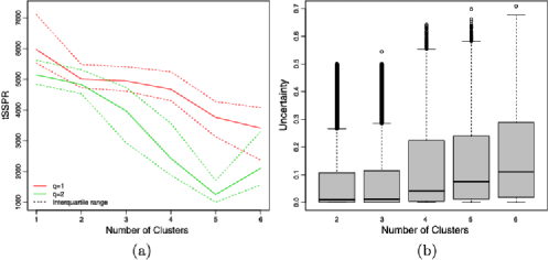
Figure 1: Assessing model fit. (a) The median tSSPR, and its associated uncertainty, across a range of MFA-MD models. (b) Box plots of clustering uncertainty across models with between 2 and 6 clusters, and a 1-dimensional latent trait.

Based on the median tSSPR values, the improvement in fit from $q=1$ to $q=2$ across $G$ was felt to be insufficient to substantiate focusing on the $q=2$ models, given the reduction in parsimony. Examination of the parameters of the $q=2$ model for a fixed $G$ also provided little substantive insight over the $q=1$ model. Models with $G=2$, $G=3$ and $G=4$ (with $q=1$) all seem to fit equivalently well; this observation is also apparent under other truncation levels $T$, as illustrated in McParland et al. (2014a). Further, the median tSSPR values support the literature’s assertion that SES clusters exist, that is, that $G>1$.

5.1.2 Clustering uncertainty

Clustering uncertainty [Bensmail et al. (1997), Gormley and Murphy (2006)] is an exploratory tool which helps assess models in the context of clustering. The uncertainty with which household $i$ is assigned to its cluster may be estimated by

$$U_{i}=\min_{g=1,\ldots,G}\bigl{\{}1-\mathbb{P}(\mbox{cluster }g|\mbox{household }i)\bigr{\}}.$$

If household $i$ is strongly associated with cluster $g$, then $U_{i}$ will be small.

Box plots of the clustering uncertainty of each household under models with $G=2,\ldots,6$ (and $q=1$) are shown in Figure 1(b). The uncertainty values are low in general, indicating that households are assigned to clusters with a high degree of confidence. Low values are observed for the $G=2$ and $G=3$ models, with a notable increase for higher numbers of clusters.

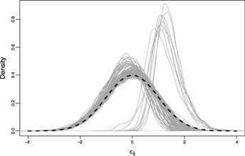
Figure 2: Bayesian latent residuals, corresponding to the cattle survey item, for 100 randomly sampled households under the $G=3$ model with a 1-dimensional latent trait. The dashed black line is the standard normal curve.

5.1.3 Bayesian latent residuals analysis

The posterior predictive checks and the clustering uncertainties suggest that models with $G=2$, $G=3$ and $G=4$ (and $q=1)$ appear to fit well and are relatively parsimonious. Focus is given to these models, and Bayesian latent residuals [Johnson and Albert (1999), Fox (2010)] are employed to investigate their model fit. Bayesian latent residuals, defined by $\varepsilon_{ij}=z_{ij}-\tilde{\underline{\lambda}}{}_{gj}^{T}\tilde{\underline{\theta}}_{i}$, should follow a standard normal distribution. The Bayesian latent residuals follow their theoretical distribution reasonably well for the three models under focus; Figure 2 shows kernel density estimate curves of the Bayesian latent residuals corresponding to the cattle item for a random sample of 100 households. The curves are estimated based on the residuals at each MCMC iteration. Residuals which do not appear to follow a standard normal distribution correspond to responses which were unusual given the household’s cluster membership. Further examples of such residual plots are given in McParland et al. (2014a).

The three approaches to assessing model fit suggest that focus should be given to models with $G=2$, $G=3$ and $G=4$, and $q=1$. As the $G=3$ and $G=4$ models give deeper insight to the SES structure of the Agincourt households than the $G=2$ model, the $G=3$ model is explored in detail in Section 5.2; a substantive comparison with the $G=4$ model is provided in Section 5.3, in which the $G=2$ model is also discussed.

5.2 Results: Three-component MFA-MD model

The clustering resulting from fitting a $3$-component MFA-MD model, with a one-dimensional latent trait, divides the Agincourt households into $3$ distinct homogeneous subpopulations, with intuitive socio-economic characteristics.

The conditional probability that household $i$ belongs to cluster $g$ can be estimated from the MCMC samples by dividing the number of times household $i$ was allocated to group $g$ by the number of samples. A “hard” clustering is then obtained by considering $\max_{g}\mathbb{P}(\mbox{cluster }g|\mbox{household }i)$, $\forall i$, and assigning households to the cluster for which this maximum is achieved.

Table 1: The cardinality of each group and the modal response to items on which the modal response differs across groups

G	1	2	3
#	7864	6543	3210
# Bedrooms	2	2	$\leq$1
Separate Living Area	Yes	Yes	No
Toilet Facilities	Yard	Yard	Bush
Toilet Type	Pit	Pit	None
Power for Cooking	Electric	Wood	Wood
Stove	Yes	No	No
Fridge	Yes	Yes	No
Television	Yes	Yes	No
Video	Yes	No	No
Poultry	No	Yes	No

The modal responses to items for which the modal response differed across groups are presented in Table 1. These statistics only tell part of the story, however, and the distribution of responses will be analyzed later.

It can be seen from Table 1 that cluster 1 is a modern/wealthy group of households. The modal responses indicate that households in this cluster are most likely to possess modern conveniences such as a stove, a fridge and also some luxury items such as a television.

In contrast, cluster 3 is a less wealthy group. Households in this group are likely to have poor sanitary facilities—the modal response to the location of toilet facilities and the type of toilet are “bush” and “none,” respectively. Households in cluster 3 are also less likely to own modern conveniences such as a fridge or television.

The socio-economic status of cluster 2 is somewhere between that of the other two groups, but closer to cluster 1 than 3. Households in cluster 2 are likely to have better sewage facilities and larger dwellings than those in cluster 3 but lack some luxury assets such as a video player. They are also likely to keep poultry and cook with wood rather than electricity, which suggests this group may be less modern than cluster 1 to some degree.

It is interesting to note that the largest group is the wealthy/modern cluster 1, while the smallest group is cluster 3 who have the lowest living standards.

An almost identical table to Table 1 was produced for a 3-component model with a 2-dimensional latent trait. There were some further differences in the Power for Lighting and Cell Phone items but the clusters have the same substantive interpretation.

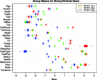
Figure 3: Box plots of MCMC samples of the dimensions of the cluster means, $\underline{\mu}{}_{g}$, corresponding to binary and ordinal items.

A more detailed picture of how the groups differ from each other is presented in Figures 3 and 4. Box plots of the MCMC samples of the cluster specific mean parameter $\underline{\mu}{}_{g}$ are shown in these figures. The box plots for the binary/ordinal items (Figure 3) have a different interpretation to those for the nominal items (Figure 4). The binary and ordinal responses have been coded with the convention that larger responses correspond to greater wealth. Thus, a higher mean value for the latent data corresponding to these items is indicative of greater wealth. To interpret the box plots for the nominal items, all latent dimensions for a particular item must be considered. If the mean of one dimension ($k$, say) is greater than the means of the others for a particular cluster, then the response corresponding to dimension $k$ is the most likely response within that cluster. If the means for all dimensions for a particular item are less than $0$, then the most likely response by households in that cluster is the first choice.

The box plots corresponding to the binary and ordinal items are shown in Figure 3. The elements of the mean of cluster 1 (the wealthy/modern cluster) $\underline{\mu}{}_{1}$ can be seen to be greater than those for the other clusters in general; this reflects the greater wealth observed in cluster 1 compared to the other groups. Similarly, the elements of $\underline{\mu}{}_{3}$ (the least wealthy group) are lower than those for the other groups, reflecting the lower socio-economic status of households in cluster 3. The difference between cluster 3 and clusters 1 and 2 is particularly stark on the location of toilet facilities (ToiletFac) and the type of toilet facilities (ToiletType) items. The means for clusters 1 and 2 are notably higher than the mean for cluster 3 since the responses for groups 1 and 2 are typically a number of categories higher on these items.

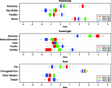
Figure 4: Box plots of MCMC samples of the dimensions of the cluster means, $\underline{\mu}{}_{g}$, corresponding to nominal items. The first plot shows box plots of the means of the latent dimensions relating to the PowerCook item, the second shows the means of the dimensions representing the PowerLight item and the third shows the means of the dimensions corresponding to the Roof item.

Figure 4 shows box plots of the MCMC samples of the dimensions of the cluster mean parameters, $\underline{\mu}{}_{g}$, corresponding to the nominal items. Focusing on the latent dimensions corresponding to the PowerCook item, say, it can be seen that the highest mean for cluster 1 is on the “electricity” dimension followed closely by the “wood” dimension, and that these means are greater than $0$. This implies that the most likely response to the PowerCook item for cluster 1 is electricity but that a significant proportion of the households in this group cook with wood. The highest means for clusters 2 and 3 are on the “wood” latent dimension. Thus, most of the households in these clusters cook with wood in contrast to the wealthy/modern cluster 1. This difference is indicative of a socio-economic divide. In a similar way, the mean parameters for the PowerLight item suggest that electricity is the most likely source of power for lighting for households in all clusters; the parameter estimates associated with the Roof item suggest corrugated iron roofs are the predominant roofing type on dwellings in the Agincourt region.

To further investigate the difference between the $3$ clusters, the response probabilities to individual survey items within a cluster are examined. For example, Table 2 shows the probability of observing each possible response to the Stove item, conditional on the members of each cluster.

=150pt G No Yes 1 0.005 0.995 2 0.509 0.491 3 0.626 0.374

Table 2: Cluster specific response probabilities to the survey item Stove

Figure 5: Pairwise comparisons of groups using Hellinger distance. (a) Hellinger distances between groups 1 and 2. Total distance is 3.544. (b) Hellinger distances between groups 1 and 3. Total distance is 7.316. (c) Hellinger distances between groups 2 and 3. Total distance is 5.643.

The distances between the cluster specific item response probability vectors can be used to make pairwise comparisons of groups. The distance measure used here is Hellinger distance [Le Cam and Yang (1990), Rao (1995), Bishop (2006)]. Pairwise comparisons between clusters are illustrated in Figure 5. The Hellinger distance between response probability vectors for each item is plotted. The groups that are most different are clusters 1 (the wealthy/modern cluster) and 3 (the least wealthy cluster). The sum of the Hellinger distances between these groups across all items is 7.316. The items for which the Hellinger distance between the response probability vectors is largest are ToiletType, ToiletFac, Stove and PowerLight, highlighting the areas in which households in these clusters differ most. There are noteworthy Hellinger distances for many other items also. The difference in response patterns for these items is also evident in the box plots in Figures 3 and 4.

The sum of the Hellinger distances between clusters 1 and 2 (the wealthier two clusters) across all items is 3.544, making these two groups the most similar. There are some notable differences, however, the Hellinger distance between the groups on the items Stove and PowerCook are 0.501 and 0.556, respectively, which accounts for almost $30\%$ of the total distance.

Clusters 2 and 3 are quite different and the sum of the Hellinger distances between these groups is 5.643. As was the case for clusters 1 and 3, the items ToiletType and ToiletFac provide the largest Hellinger distances between groups 2 and 3. In contrast, however, there are much smaller differences for the items Stove and PowerCook. Again these results highlight the specific areas in which the socio-economic status of households within each cluster differ. A similar pattern was observed in Table 1 and Figures 3 and 4.

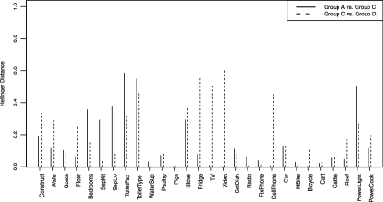
Figure 6: Hellinger distances between groups A and C (red) and groups C and D (blue). The total distances are 4.219 and 5.699 respectively.

5.3 Results: Four- and two-component MFA-MD models

Many of the substantive results returned by the 4-component model are similar to those inferred from the 3-component model. Notably, the items listed in Table 1 (i.e., those items for which the modal response differs across groups in the 3-component solution) are a subset of those items for which the modal response differs across groups in the 4-component solution [details provided in McParland et al. (2014a)]. Groups A, B and C in the 4-component model are substantively similar to groups 1, 2 and 3 from the 3-component model, respectively. Group D returned by the 4-component model is interesting, however. It is similar to group A in that households in this cluster possess many modern conveniences but the standard of their dwelling is not at the same level as those in group A. The standard of dwellings in group D is similar to those in group C, however, the households differ from group C in terms of the modern conveniences they possess. Further investigation revealed that households in group C are either in group 1 (wealthy) or group 3 (poor) of the 3-component solution. Figure 6 plots the Hellinger distance between groups A and C and groups C and D, illustrating the differences and similarities between these clusters. It can be seen that the largest distances between groups A and C concern items related to the dwelling while the largest distances between groups C and D concern modern convenience ownership.

Interestingly, group 2 and group B, under the 3- and 4-component solutions, respectively, consist of almost exactly the same households. These groups are deemed to be wealthy but less modern than group 1 and group A, under the 3- and 4-component solutions, respectively. Indeed, under the 5- and 6-component models, the essence of this cluster remains intact.

Similar substantive results are inferred from the two-component MFA-MD solution. Again, it is notable that those items for which the modal response differs across groups in the 2-component solution [detailed in McParland et al. (2014a)] are a subset of those items for which the modal response differs across groups in the 3-component solution (detailed in Table 1). Groups A and B under the 2-component solution relate generally to clusters 1 and 2 in the 3-component solution. The poorer cluster B in the 2-component solution separates to create clusters 2 and 3 in the 3-component solution.

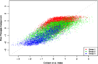
Figure 7: Comparing the principal component based approach of Filmer and Pritchett (2001) to the asset index of Collinson et al. (2009). The gray line shows where both scores are equal and the points are colored according to the 3 group, 1-dimensional latent trait, MFA-MD solution.

5.4 Comparison to existing methodology

Several other approaches to exploring the SES landscape based on asset survey data are detailed in the demography literature. It is therefore of interest to compare the results obtained when exploring the Agincourt SES landscape using the proposed MFA-MD model to those obtained when existing methods are applied. In particular, two existing methods for analyzing mixed type socio-economic data are considered, that of Filmer and Pritchett (2001) and that of Collinson et al. (2009), mentioned in Section 2.

The Filmer and Pritchett (2001) approach codes ordinal and nominal responses using dummy binary variables and a principal component analysis (PCA) is applied to the resulting data matrix. The Collinson et al. (2009) approach constructs a continuous asset index from the raw data. Figure 7 shows the standardized first principal component scores plotted against the standardized asset index of Collinson et al. (2009) when these methods were applied to the Agincourt data. The points are colored by the three-group clustering solution considered here. The two alternative scores do seem to broadly agree. In addition, the 3-cluster solution appears to roughly correspond to the gradation of the first principal component scores. However, Filmer and Pritchett (2001) partition households into the lowest 40%, middle 40% and top 20% based on these principal component scores; their choice of percentiles is arbitrary. Comparing the allocation based on this criterion to that from our model results in a Rand and adjusted Rand index of 0.61 and 0.15, respectively. Thus, the clustering solution using the MFA-MD model is quite different than that currently in use. Clustering households is not the primary goal for Collinson et al. (2009), though they do classify households as “chronically poor” if they have below the median asset index score. The MFA-MD model allocates households using a more preferable objective model-based approach, while recognizing the different data types and treating them accordingly.

6 Discussion

This paper set out to describe and understand the SES landscape in the Agincourt region in South Africa through clustering households based on their asset status survey data. The MFA-MD model described in this paper successfully achieved this aim by clustering households into groups of differing socio-economic status. Which households are in each group and what differentiates these clusters from each other can be examined in the model output. This information is potentially of great benefit to various authorities in the Agincourt region. The interpretation of the SES clusters could aid decision-making with regard to infrastructural development and other social policy. Further, the resulting clustering memberships and cluster interpretations will be used to aid targeted sampling of a particular cluster of households in the Agincourt region in future surveys. New questions in future surveys can be derived based on the substantive information now known about the SES clusters. The clustering output from the MFA-MD model could also be used as covariate input to other models, such as mortality models. There may be important differences in mortality rates in different socio-economic strata within the region; new health policies may need to take these differences into account. A key interest for the sociologists studying the Agincourt region is understanding social mobility, and substantively examining SES clusters is the first step in this process. Thus, the clustering exploration of the SES landscape in Agincourt will provide support to researchers in the Agincourt region, through the exposure of (dis)similar features of the clusters of households. The information provided about the SES Agincourt landscape is based on a statistically principled clustering approach, rather than ad hoc measures.

The MFA-MD model also provides a novel model-based approach to clustering mixed categorical data. The SES data used here is a mix of binary, ordinal and nominal data. The MFA-MD model provides clustering capabilities in the context of such mixed data without mistreating any one data type. A factor analytic model is fitted to each group individually and may be interpreted in the usual manner.

Future research directions are plentiful and varied. The lack of a formal model selection criterion for the MFA-MD model is the most pressing, and challenging. The provision of a formal criterion would facilitate application of the MFA-MD model in settings in which an optimal model must be selected; a formal criterion which selects the most appropriate number of components and also the dimension of the latent trait would be very beneficial. Model selection tools based on the marginal likelihood [Friel and Wyse (2011)] are a natural approach to model selection within the Bayesian paradigm, but the intractable likelihood of the observed data $Y$ poses difficulties for the MFA-MD model. This renders even approximate approaches such as BIC unusable. One alternative would be to approximate the observed likelihood using the underlying latent data $Z$, but this also brings difficulties and uncertainty [McParland and Gormley (2013)]. Other joint approaches to clustering and choosing the number of components are popular in the literature; using a Dirichlet process mixture model or incorporating reversible jump MCMC may provide fruitful future research directions. However, the applied nature of the work here and the requirement of interpretative clusters and model parameters motivated the use of a finite mixture model. Approaches to choosing the number of latent factors such as those considered in Lopes and West (2004) or Bhattacharya and Dunson (2011) could also have potential within the MFA-MD context.

Additionally, there are several ways in which the MFA-MD model itself could be extended. Here, the last time point from the Agincourt survey was analyzed. However, there have been several waves of this particular survey—extending the MFA-MD model to appropriately model longitudinal data would be beneficial. In this way the Agincourt households could be tracked across time, as they may or may not move between socio-economic strata. As with most clustering models, the variables included in the model are potentially influential. The addition of a variable selection method within the context of the MFA-MD model could significantly improve clustering performance and provide substantive insight to asset indicators of SES. A reduction in the number of variables would also decrease the computational time required to fit such models. In a similar vein, the Metropolis–Hastings step required to sample the threshold parameters in the current model fitting approach could potentially be removed by using a rank likelihood approach [Hoff (2009)]. This could also offer an improvement in computational time.

Other areas of ongoing and future work include the inclusion of modeling continuous data by the MFA-MD model. This would facilitate the clustering of mixed data consisting of both continuous and categorical data [McParland et al. (2014b)], and requires little extension to the MFA-MD model proposed here. Allowing further correlations in the latent variable beyond those produced by the latent trait is an interesting model extension; this could be achieved by relaxing the unit variance in the probit link. Finally, covariate information could naturally be incorporated in the MFA-MD model in the mixture of experts framework [Gormley and Murphy (2008), Jacobs et al. (1991)]; such an approach could be insightful in understanding cause-effect relationships in the Agincourt SES clusters and should be a straightforward extension.

Table 3: A list of all survey items and the possible responses. The final three items in the table are regarded as nominal, all other items are binary or ordinal

Item	Description	Response options
Construct	Indicates whether main dwelling is still	(No, Yes)
	under construction.
Walls	Construction materials used for walls.	(Informal, Modern)
Floor	Construction materials used for floor.	(Informal, Modern)
Bedrooms	Number of bedrooms in the household.	($\leq$1, 2, 3, 4, 5, $\geq$6)
SepKit	Indicates whether kitchen is separate	(No, Yes)
	from sleeping area.
SepLiv	Indicates whether living room is separate	(No, Yes)
	from sleeping area.
ToiletFac	Reports the physical location of toilet in	(Bush, Other House,
	the household.	In Yard, In House )
ToiletType	Reports the type of toilet used.	(None, Pit, VIP, Modern)
WaterSup	Reports the water supply source.	(From a tap, Other)
Stove	Reports stove ownership status.	(No, Yes)
Fridge	Reports fridge ownership status.	(No, Yes)
TV	Reports television ownership status.	(No, Yes)
Video	Reports video player ownership status.	(No, Yes)
SatDish	Reports satellite dish ownership status.	(No, Yes)
Radio	Reports radio ownership status.	(No, Yes)
FixPhone	Reports fixed phone ownership status.	(No, Yes)
CellPhone	Reports mobile phone ownership status.	(No, Yes)
Car	Reports car ownership status.	(No, Yes)
MBike	Reports motor bike ownership status.	(No, Yes)
Bicycle	Reports bicycle ownership status.	(No, Yes)
Cart	Reports animal drawn cart ownership	(No, Yes)
	status.
Cattle	Reports cattle ownership status.	(No, Yes)
Goats	Reports goats ownership status.	(No, Yes)
Poultry	Reports poultry ownership status.	(No, Yes)
Pigs	Reports pig ownership status.	(No, Yes)
Roof	Construction materials used for roof.	(Other informal, Thatch,
		Other modern,
		Corrugated iron, Tile)
PowerLight	Main power supply for lights	(Other, Candles, Paraffin,
	and appliances.	Solar, Battery/Generator,
		Electricity)
PowerCook	Main power supply for cooking.	(Other, Wood, Paraffin,
		Gas Bottle, Electricity)

Appendix A Survey items

Appendix B Latent variable formulation of nominal responses

Suppose item $j$ is nominal with $K_{j}=3$ options: apple (denoted level 1), banana (denoted level 2) or pear (denoted level 3). Thus, $\underline{z}_{ij}=\{z_{ij}^{1},z_{ij}^{2}\}$.

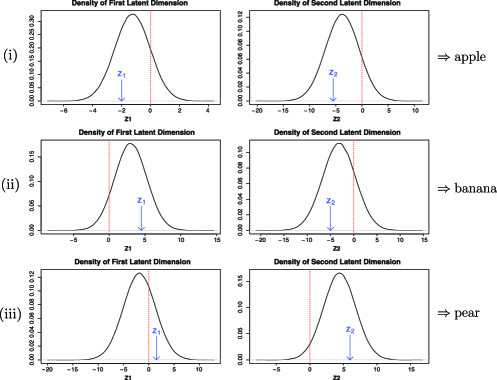
Figure 8: Latent variable formulation of nominal responses.

Figure 8 shows what the marginal distributions of the latent variables might look like along with realizations from those distributions: [(iii)]

Both $z_{ij}^{1}$ and $z_{ij}^{2}$ are less than 0, thus $\max_{k}\{z_{ij}^{k}\}<0\Rightarrow y_{ij}=1$, that is, apple.

$z_{ij}^{1}=\max_{k}\{z_{ij}^{k}\}$ and $z_{ij}^{1}>0\Rightarrow y_{ij}=2,\mbox{ that is, banana}$.

$z_{ij}^{2}=\max_{k}\{z_{ij}^{k}\}$ and $z_{ij}^{2}>0\Rightarrow y_{ij}=3,\mbox{ that is, pear}$. In the MCMC algorithm, these latent variables are sampled conditional on the observed data $Y$. Given the nominal response, the full conditional distributions are truncated appropriately.

Appendix C Convergence of Markov chains

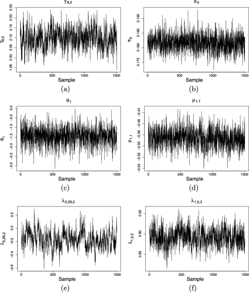
Figure 9: Trace plots of Markov chains for selected parameters. The plots shown are of the thinned MCMC samples, post burn-in. (a) Trace plot of the MCMC samples for one of the threshold parameters of the $\mathit{ToiletFac}$ item. (b) Trace plot of the MCMC samples of the mixing weight for group 3. (c) Trace plot of the MCMC samples for the latent trait of the first household. (d) Trace plot of the MCMC samples of the first dimension of the mean vector for group 1. (e) Trace plot of the MCMC samples of one of the loadings parameters for nominal item $\mathit{Roof}$. (f) Trace plot of the MCMC samples of the loadings parameter for ordinal item $\mathit{Bedrooms}$.

References

- Aguilar and West (2000) {barticle}[author] \bauthor\bsnmAguilar, \bfnmO.\binitsO. and \bauthor\bsnmWest, \bfnmM.\binitsM. (\byear2000). \btitleBayesian dynamic factor models and portfolio allocation. \bjournalJ. Bus. Econom. Statist. \bvolume18 \bpages338–357. \bptokimsref\endbibitem
- Albert and Chib (1993) {barticle}[mr] \bauthor\bsnmAlbert, \bfnmJames H.\binitsJ. H. and \bauthor\bsnmChib, \bfnmSiddhartha\binitsS. (\byear1993). \btitleBayesian analysis of binary and polychotomous response data. \bjournalJ. Amer. Statist. Assoc. \bvolume88 \bpages669–679. \bidissn=0162-1459, mr=1224394 \bptokimsref\endbibitem
- Alkema et al. (2008) {bmisc}[author] \bauthor\bsnmAlkema, \bfnmL.\binitsL., \bauthor\bsnmFaye, \bfnmO.\binitsO., \bauthor\bsnmMutua, \bfnmM.\binitsM. and \bauthor\bsnmZulu, \bfnmE.\binitsE. (\byear2008). \bhowpublishedIdentifying poverty groups in Nairobi’s slum settlements: A latent class analysis approach. In Conference Paper for Annual Meeting of the Population Association of America. New Orleans. \bptokimsref\endbibitem
- Bensmail et al. (1997) {barticle}[author] \bauthor\bsnmBensmail, \bfnmH.\binitsH., \bauthor\bsnmCeleux, \bfnmG.\binitsG., \bauthor\bsnmRaftery, \bfnmA. E.\binitsA. E. and \bauthor\bsnmRobert, \bfnmC. P.\binitsC. P. (\byear1997). \btitleInference in model-based cluster analysis. \bjournalStatist. Comput. \bvolume7 \bpages1–10. \bptokimsref\endbibitem
- Bhattacharya and Dunson (2011) {barticle}[mr] \bauthor\bsnmBhattacharya, \bfnmA.\binitsA. and \bauthor\bsnmDunson, \bfnmD. B.\binitsD. B. (\byear2011). \btitleSparse Bayesian infinite factor models. \bjournalBiometrika \bvolume98 \bpages291–306. \biddoi=10.1093/biomet/asr013, issn=0006-3444, mr=2806429 \bptokimsref\endbibitem
- Bishop (2006) {bbook}[mr] \bauthor\bsnmBishop, \bfnmChristopher M.\binitsC. M. (\byear2006). \btitlePattern Recognition and Machine Learning. \bpublisherSpringer, \blocationNew York. \biddoi=10.1007/978-0-387-45528-0, mr=2247587 \bptokimsref\endbibitem
- Browne and McNicholas (2012) {barticle}[mr] \bauthor\bsnmBrowne, \bfnmRyan P.\binitsR. P. and \bauthor\bsnmMcNicholas, \bfnmPaul D.\binitsP. D. (\byear2012). \btitleModel-based clustering, classification, and discriminant analysis of data with mixed type. \bjournalJ. Statist. Plann. Inference \bvolume142 \bpages2976–2984. \biddoi=10.1016/j.jspi.2012.05.001, issn=0378-3758, mr=2943769 \bptokimsref\endbibitem
- Cai et al. (2011) {barticle}[mr] \bauthor\bsnmCai, \bfnmJing-Heng\binitsJ.-H., \bauthor\bsnmSong, \bfnmXin-Yuan\binitsX.-Y., \bauthor\bsnmLam, \bfnmKwok-Hap\binitsK.-H. and \bauthor\bsnmIp, \bfnmEdward Hak-Sing\binitsE. H.-S. (\byear2011). \btitleA mixture of generalized latent variable models for mixed mode and heterogeneous data. \bjournalComput. Statist. Data Anal. \bvolume55 \bpages2889–2907. \biddoi=10.1016/j.csda.2011.05.011, issn=0167-9473, mr=2813054 \bptokimsref\endbibitem
- Celeux, Hurn and Robert (2000) {barticle}[mr] \bauthor\bsnmCeleux, \bfnmGilles\binitsG., \bauthor\bsnmHurn, \bfnmMerrilee\binitsM. and \bauthor\bsnmRobert, \bfnmChristian P.\binitsC. P. (\byear2000). \btitleComputational and inferential difficulties with mixture posterior distributions. \bjournalJ. Amer. Statist. Assoc. \bvolume95 \bpages957–970. \biddoi=10.2307/2669477, issn=0162-1459, mr=1804450 \bptokimsref\endbibitem
- Chib, Greenberg and Chen (1998) {bmisc}[author] \bauthor\bsnmChib, \bfnmS.\binitsS., \bauthor\bsnmGreenberg, \bfnmE.\binitsE. and \bauthor\bsnmChen, \bfnmY.\binitsY. (\byear1998). \bhowpublishedMCMC methods for fitting and comparing multinomial response models. Technical report, Washington Univ. in St. Louis. \bptokimsref\endbibitem
- Collinson et al. (2009) {bmisc}[author] \bauthor\bsnmCollinson, \bfnmM. A.\binitsM. A., \bauthor\bsnmClark, \bfnmS. J.\binitsS. J., \bauthor\bsnmGerritsen, \bfnmA. A. M.\binitsA. A. M., \bauthor\bsnmByass, \bfnmP.\binitsP., \bauthor\bsnmKahn, \bfnmK.\binitsK. and \bauthor\bsnmTollmann, \bfnmS. M.\binitsS. M. (\byear2009). \bhowpublishedThe dynamics of poverty and migration in a rural south african community, 2001–2005. Technical report, Center for Statistics and the Social Sciences Univ. of Washington. \bptokimsref\endbibitem
- Cowles (1996) {barticle}[author] \bauthor\bsnmCowles, \bfnmM. K.\binitsM. K. (\byear1996). \btitleAccelerating Monte Carlo Markov chain convergence for cumulative-link generalized linear models. \bjournalStatist. Comput. \bvolume6 \bpages101–111. \bptokimsref\endbibitem
- Erikson and Goldthorpe (1992) {bbook}[author] \bauthor\bsnmErikson, \bfnmR.\binitsR. and \bauthor\bsnmGoldthorpe, \bfnmJ. H.\binitsJ. H. (\byear1992). \btitleThe Constant Flux: A Study of Class Mobility in Industrial Societies. \bpublisherOxford Univ. Press, \blocationLondon. \bptokimsref\endbibitem
- Erosheva, Fienberg and Joutard (2007) {barticle}[mr] \bauthor\bsnmErosheva, \bfnmElena A.\binitsE. A., \bauthor\bsnmFienberg, \bfnmStephen E.\binitsS. E. and \bauthor\bsnmJoutard, \bfnmCyrille\binitsC. (\byear2007). \btitleDescribing disability through individual-level mixture models for multivariate binary data. \bjournalAnn. Appl. Stat. \bvolume1 \bpages502–537. \biddoi=10.1214/07-AOAS126, issn=1932-6157, mr=2415745 \bptokimsref\endbibitem
- Everitt (1988) {barticle}[mr] \bauthor\bsnmEveritt, \bfnmB. S.\binitsB. S. (\byear1988). \btitleA finite mixture model for the clustering of mixed-mode data. \bjournalStatist. Probab. Lett. \bvolume6 \bpages305–309. \biddoi=10.1016/0167-7152(88)90004-1, issn=0167-7152, mr=0933287 \bptokimsref\endbibitem
- Everitt and Merette (1988) {barticle}[author] \bauthor\bsnmEveritt, \bfnmB. S.\binitsB. S. and \bauthor\bsnmMerette, \bfnmC.\binitsC. (\byear1988). \btitleThe clustering of mixed-mode data: A comparison of possible approaches. \bjournalJ. Appl. Stat. \bvolume17 \bpages283–297. \bptokimsref\endbibitem
- Filmer and Pritchett (2001) {barticle}[author] \bauthor\bsnmFilmer, \bfnmD.\binitsD. and \bauthor\bsnmPritchett, \bfnmL. H.\binitsL. H. (\byear2001). \btitleEstimating wealth effects without expenditure data—Or tears: An application to educational enrollments in states of India. \bjournalDemography \bvolume38 \bpages115–132. \bptokimsref\endbibitem
- Fokoue and Titterington (2003) {barticle}[author] \bauthor\bsnmFokoue, \bfnmE.\binitsE. and \bauthor\bsnmTitterington, \bfnmD. M.\binitsD. M. (\byear2003). \btitleMixtures of factor analysers. Bayesian estimation and inference by stochastic simulation. \bjournalMachine Learning \bvolume50 \bpages73–94. \bptokimsref\endbibitem
- Fox (2010) {bbook}[mr] \bauthor\bsnmFox, \bfnmJean-Paul\binitsJ.-P. (\byear2010). \btitleBayesian Item Response Modeling: Theory and Applications. \bpublisherSpringer, \blocationNew York. \biddoi=10.1007/978-1-4419-0742-4, mr=2657265 \bptokimsref\endbibitem
- Fraley and Raftery (1998) {barticle}[author] \bauthor\bsnmFraley, \bfnmC.\binitsC. and \bauthor\bsnmRaftery, \bfnmA. E.\binitsA. E. (\byear1998). \btitleHow many clusters? Which clustering methods? Answers via model-based cluster analysis. \bjournalComputer Journal \bvolume41 \bpages578–588. \bptokimsref\endbibitem
- Friel and Wyse (2011) {barticle}[author] \bauthor\bsnmFriel, \bfnmN.\binitsN. and \bauthor\bsnmWyse, \bfnmJ.\binitsJ. (\byear2011). \btitleEstimating the evidence—A review. \bjournalStat. Neerl. \bvolume66 \bpages288–308. \bidmr=2955421 \bptokimsref\endbibitem
- Frühwirth-Schnatter (2006) {bbook}[mr] \bauthor\bsnmFrühwirth-Schnatter, \bfnmSylvia\binitsS. (\byear2006). \btitleFinite Mixture and Markov Switching Models. \bpublisherSpringer, \blocationNew York. \bidmr=2265601 \bptokimsref\endbibitem
- Gelman et al. (2003) {bbook}[author] \bauthor\bsnmGelman, \bfnmA.\binitsA., \bauthor\bsnmCarlin, \bfnmJ. B.\binitsJ. B., \bauthor\bsnmStern, \bfnmH. S.\binitsH. S. and \bauthor\bsnmRubin, \bfnmD. B.\binitsD. B. (\byear2003). \btitleBayesian Data Analysis. \bpublisherChapman & Hall/CRC, \blocationLondon. \bptokimsref\endbibitem
- Geweke, Keane and Runkle (1994) {barticle}[author] \bauthor\bsnmGeweke, \bfnmJ.\binitsJ., \bauthor\bsnmKeane, \bfnmM.\binitsM. and \bauthor\bsnmRunkle, \bfnmD.\binitsD. (\byear1994). \btitleAlternative computational approaches to inference in the multinomial probit model. \bjournalThe Review of Economics and Statistics \bvolume76 \bpages609–632. \bptokimsref\endbibitem
- Geweke and Zhou (1996) {barticle}[author] \bauthor\bsnmGeweke, \bfnmJ. F.\binitsJ. F. and \bauthor\bsnmZhou, \bfnmG.\binitsG. (\byear1996). \btitleMeasuring the pricing error of arbitrage pricing theory. \bjournalReview of Financial Studies \bvolume9 \bpages557–587. \bptokimsref\endbibitem
- Ghahramani and Hinton (1997) {bmisc}[author] \bauthor\bsnmGhahramani, \bfnmZ.\binitsZ. and \bauthor\bsnmHinton, \bfnmG. E.\binitsG. E. (\byear1997). \bhowpublishedThe EM algorithm for mixtures of factor analyzers. Technical report, Univ. Toronto. \bptokimsref\endbibitem
- Gollini and Murphy (2013) {barticle}[author] \bauthor\bsnmGollini, \bfnmIsabella\binitsI. and \bauthor\bsnmMurphy, \bfnmThomas Brendan\binitsT. B. (\byear2013). \btitleMixture of latent trait analyzers for model-based clustering of categorical data. \bjournalStatist. Comput. \bpages1–20. \bptokimsref\endbibitem
- Gormley and Murphy (2006) {barticle}[mr] \bauthor\bsnmGormley, \bfnmIsobel Claire\binitsI. C. and \bauthor\bsnmMurphy, \bfnmThomas Brendan\binitsT. B. (\byear2006). \btitleAnalysis of Irish third-level college applications data. \bjournalJ. Roy. Statist. Soc. Ser. A \bvolume169 \bpages361–379. \biddoi=10.1111/j.1467-985X.2006.00412.x, issn=0964-1998, mr=2225548 \bptokimsref\endbibitem
- Gormley and Murphy (2008) {barticle}[mr] \bauthor\bsnmGormley, \bfnmIsobel Claire\binitsI. C. and \bauthor\bsnmMurphy, \bfnmThomas Brendan\binitsT. B. (\byear2008). \btitleA mixture of experts model for rank data with applications in election studies. \bjournalAnn. Appl. Stat. \bvolume2 \bpages1452–1477. \biddoi=10.1214/08-AOAS178, issn=1932-6157, mr=2655667 \bptokimsref\endbibitem
- Gruhl, Erosheva and Crane (2013) {barticle}[mr] \bauthor\bsnmGruhl, \bfnmJonathan\binitsJ., \bauthor\bsnmErosheva, \bfnmElena A.\binitsE. A. and \bauthor\bsnmCrane, \bfnmPaul K.\binitsP. K. (\byear2013). \btitleA semiparametric approach to mixed outcome latent variable models: Estimating the association between cognition and regional brain volumes. \bjournalAnn. Appl. Stat. \bvolume7 \bpages2361–2383. \biddoi=10.1214/13-AOAS675, issn=1932-6157, mr=3161726 \bptokimsref\endbibitem
- Gwatkin et al. (2007) {bmisc}[author] \bauthor\bsnmGwatkin, \bfnmD. R.\binitsD. R., \bauthor\bsnmRutstein, \bfnmS.\binitsS., \bauthor\bsnmJohnson, \bfnmK.\binitsK., \bauthor\bsnmSuliman, \bfnmE.\binitsE., \bauthor\bsnmWagstaff, \bfnmA.\binitsA. and \bauthor\bsnmAmouzou, \bfnmA.\binitsA. (\byear2007). \bhowpublishedSocio-economic differences in health, nutrition, and population within developing countries: An Overview. Country Reports on HNP and Poverty, The World Bank, Washington, DC. \bptokimsref\endbibitem
- Handcock, Raftery and Tantrum (2007) {barticle}[mr] \bauthor\bsnmHandcock, \bfnmMark S.\binitsM. S., \bauthor\bsnmRaftery, \bfnmAdrian E.\binitsA. E. and \bauthor\bsnmTantrum, \bfnmJeremy M.\binitsJ. M. (\byear2007). \btitleModel-based clustering for social networks. \bjournalJ. Roy. Statist. Soc. Ser. A \bvolume170 \bpages301–354. \biddoi=10.1111/j.1467-985X.2007.00471.x, issn=0964-1998, mr=2364300 \bptokimsref\endbibitem
- Hoff (2009) {bbook}[mr] \bauthor\bsnmHoff, \bfnmPeter D.\binitsP. D. (\byear2009). \btitleA First Course in Bayesian Statistical Methods. \bpublisherSpringer, \blocationNew York. \biddoi=10.1007/978-0-387-92407-6, mr=2648134 \bptokimsref\endbibitem
- Hoff, Raftery and Handcock (2002) {barticle}[mr] \bauthor\bsnmHoff, \bfnmPeter D.\binitsP. D., \bauthor\bsnmRaftery, \bfnmAdrian E.\binitsA. E. and \bauthor\bsnmHandcock, \bfnmMark S.\binitsM. S. (\byear2002). \btitleLatent space approaches to social network analysis. \bjournalJ. Amer. Statist. Assoc. \bvolume97 \bpages1090–1098. \biddoi=10.1198/016214502388618906, issn=0162-1459, mr=1951262 \bptokimsref\endbibitem
- Hunt and Jorgensen (1999) {barticle}[author] \bauthor\bsnmHunt, \bfnmL.\binitsL. and \bauthor\bsnmJorgensen, \bfnmM.\binitsM. (\byear1999). \btitleMixture model clustering using the MULTIMIX program. \bjournalAust. N. Z. J. Stat. \bvolume41 \bpages153–171. \bptokimsref\endbibitem
- Hunt and Jorgensen (2003) {barticle}[mr] \bauthor\bsnmHunt, \bfnmLynette\binitsL. and \bauthor\bsnmJorgensen, \bfnmMurray\binitsM. (\byear2003). \btitleMixture model clustering for mixed data with missing information. \bjournalComput. Statist. Data Anal. \bvolume41 \bpages429–440. \biddoi=10.1016/S0167-9473(02)00190-1, issn=0167-9473, mr=1973722 \bptokimsref\endbibitem
- Jacobs et al. (1991) {barticle}[author] \bauthor\bsnmJacobs, \bfnmR. A.\binitsR. A., \bauthor\bsnmJordan, \bfnmM. I.\binitsM. I., \bauthor\bsnmNowlan, \bfnmS. J.\binitsS. J. and \bauthor\bsnmHinton, \bfnmG. E.\binitsG. E. (\byear1991). \btitleAdaptive mixture of local experts. \bjournalNeural Comput. \bvolume3 \bpages79–87. \bptokimsref\endbibitem
- Johnson and Albert (1999) {bbook}[mr] \bauthor\bsnmJohnson, \bfnmValen E.\binitsV. E. and \bauthor\bsnmAlbert, \bfnmJames H.\binitsJ. H. (\byear1999). \btitleOrdinal Data Modeling. \bpublisherSpringer, \blocationNew York. \bidmr=1683018 \bptokimsref\endbibitem
- Kahn et al. (2007) {barticle}[author] \bauthor\bsnmKahn, \bfnmK.\binitsK., \bauthor\bsnmTollman, \bfnmS. M.\binitsS. M., \bauthor\bsnmCollinson, \bfnmM. A.\binitsM. A., \bauthor\bsnmClark, \bfnmS. J.\binitsS. J., \bauthor\bsnmTwine, \bfnmR.\binitsR., \bauthor\bsnmClark, \bfnmB. D.\binitsB. D., \bauthor\bsnmShabangu, \bfnmM.\binitsM., \bauthor\bsnmGómez-Olivé, \bfnmF. X.\binitsF. X., \bauthor\bsnmMokoena, \bfnmO.\binitsO. and \bauthor\bsnmGarenne, \bfnmM. L.\binitsM. L. (\byear2007). \btitleResearch into health, population and social transitions in rural South Africa: Data and methods of the Agincourt Health and Demographic Surveillance System1. \bjournalScandinavian Journal of Public Health \bvolume35 \bpages8–20. \bptokimsref\endbibitem
- Lawrence and Krzanowski (1996) {barticle}[author] \bauthor\bsnmLawrence, \bfnmC. J.\binitsC. J. and \bauthor\bsnmKrzanowski, \bfnmW. J.\binitsW. J. (\byear1996). \btitleMixture separation for mixed-mode data. \bjournalStatist. Comput. \bvolume6 \bpages85–92. \bptokimsref\endbibitem
- Le Cam and Yang (1990) {bbook}[mr] \bauthor\bsnmLe Cam, \bfnmLucien\binitsL. and \bauthor\bsnmYang, \bfnmGrace Lo\binitsG. L. (\byear1990). \btitleAsymptotics in Statistics: Some Basic Concepts. \bpublisherSpringer, \blocationNew York. \biddoi=10.1007/978-1-4684-0377-0, mr=1066869 \bptokimsref\endbibitem
- Lopes and West (2004) {barticle}[mr] \bauthor\bsnmLopes, \bfnmHedibert Freitas\binitsH. F. and \bauthor\bsnmWest, \bfnmMike\binitsM. (\byear2004). \btitleBayesian model assessment in factor analysis. \bjournalStatist. Sinica \bvolume14 \bpages41–67. \bidissn=1017-0405, mr=2036762 \bptokimsref\endbibitem
- Lord (1952) {barticle}[author] \bauthor\bsnmLord, \bfnmF. M.\binitsF. M. (\byear1952). \btitleThe relation of the reliability of multiple-choice tests to the distribution of item difficulties. \bjournalPsychometrika \bvolume17 \bpages181–194. \bptokimsref\endbibitem
- Lord and Novick (1968) {bbook}[author] \bauthor\bsnmLord, \bfnmF. M.\binitsF. M. and \bauthor\bsnmNovick, \bfnmM. R.\binitsM. R. (\byear1968). \btitleStatistical Theories of Mental Test Scores. \bpublisherAddison-Wesley, \blocationReading, MA. \bptokimsref\endbibitem
- Masters (1982) {barticle}[author] \bauthor\bsnmMasters, \bfnmG.\binitsG. (\byear1982). \btitleA Rasch model for partial credit scoring. \bjournalPsychometrika \bvolume47 \bpages149–174. \bptokimsref\endbibitem
- McCulloch and Rossi (1994) {barticle}[mr] \bauthor\bsnmMcCulloch, \bfnmRobert\binitsR. and \bauthor\bsnmRossi, \bfnmPeter E.\binitsP. E. (\byear1994). \btitleAn exact likelihood analysis of the multinomial probit model. \bjournalJ. Econometrics \bvolume64 \bpages207–240. \biddoi=10.1016/0304-4076(94)90064-7, issn=0304-4076, mr=1310524 \bptokimsref\endbibitem
- McKenzie (2005) {barticle}[author] \bauthor\bsnmMcKenzie, \bfnmD. J.\binitsD. J. (\byear2005). \btitleMeasuring inequality with asset indicators. \bjournalJournal of Population Economics \bvolume18 \bpages229–260. \bptokimsref\endbibitem
- McNicholas and Murphy (2008) {barticle}[mr] \bauthor\bsnmMcNicholas, \bfnmPaul David\binitsP. D. and \bauthor\bsnmMurphy, \bfnmThomas Brendan\binitsT. B. (\byear2008). \btitleParsimonious Gaussian mixture models. \bjournalStat. Comput. \bvolume18 \bpages285–296. \biddoi=10.1007/s11222-008-9056-0, issn=0960-3174, mr=2413385 \bptokimsref\endbibitem
- McParland and Gormley (2013) {bbook}[author] \bauthor\bsnmMcParland, \bfnmD.\binitsD. and \bauthor\bsnmGormley, \bfnmI. C.\binitsI. C. (\byear2013). \btitleClustering Ordinal Data via Latent Variable Models. \bseriesStudies in Classification, Data Analysis, and Knowledge Organization \bvolume547. \bpublisherSpringer, \blocationBerlin. \bptokimsref\endbibitem
- McParland et al. (2014a) {bmisc}[author] \bauthor\bsnmMcParland, \binitsD., \bauthor\bsnmGormley, \binitsI., \bauthor\bsnmMcCormick, \binitsT. H., \bauthor\bsnmClark, \binitsS. J., \bauthor\bsnmKabudula, \binitsC. and \bauthor\bsnmCollinson, \binitsM. A. (\byear2014a). \bhowpublishedSupplement to “Clustering South African households based on their asset status using latent variable models.” DOI:\doiurl10.1214/14-AOAS726SUPPA, DOI:\doiurl10.1214/14-AOAS726SUPPB, DOI:\doiurl10.1214/14-AOAS726SUPPC. \bptokimsref \endbibitem
- McParland et al. (2014b) {bmisc}[author] \bauthor\bsnmMcParland, \bfnmD.\binitsD., \bauthor\bsnmGormley, \bfnmI. C.\binitsI. C., \bauthor\bsnmBrennan, \bfnmL.\binitsL. and \bauthor\bsnmRoche, \bfnmH. M.\binitsH. M. (\byear2014b). \bhowpublishedClustering mixed continuous and categorical data from the LIPGENE study: Examining the interaction of nutrients and genotype in the metabolic syndrome. Technical report, Univ. College Dublin. \bptokimsref\endbibitem
- Murray et al. (2013) {barticle}[mr] \bauthor\bsnmMurray, \bfnmJared S.\binitsJ. S., \bauthor\bsnmDunson, \bfnmDavid B.\binitsD. B., \bauthor\bsnmCarin, \bfnmLawrence\binitsL. and \bauthor\bsnmLucas, \bfnmJoseph E.\binitsJ. E. (\byear2013). \btitleBayesian Gaussian copula factor models for mixed data. \bjournalJ. Amer. Statist. Assoc. \bvolume108 \bpages656–665. \biddoi=10.1080/01621459.2012.762328, issn=0162-1459, mr=3174649 \bptokimsref\endbibitem
- Muthén and Shedden (1999) {barticle}[pbm] \bauthor\bsnmMuthén, \bfnmB.\binitsB. and \bauthor\bsnmShedden, \bfnmK.\binitsK. (\byear1999). \btitleFinite mixture modeling with mixture outcomes using the EM algorithm. \bjournalBiometrics \bvolume55 \bpages463–469. \bidissn=0006-341X, pmid=11318201 \bptokimsref\endbibitem
- Nobile (1998) {barticle}[author] \bauthor\bsnmNobile, \bfnmA.\binitsA. (\byear1998). \btitleA hybrid Markov chain for the Bayesian analysis of the multinomial probit model. \bjournalStatist. Comput. \bvolume8 \bpages229–242. \bptokimsref\endbibitem
- Quinn (2004) {barticle}[author] \bauthor\bsnmQuinn, \bfnmK. M.\binitsK. M. (\byear2004). \btitleBayesian factor analysis for mixed ordinal and continuous responses. \bjournalPolitical Analysis \bvolume12 \bpages338–353. \bptokimsref\endbibitem
- Rao (1995) {barticle}[mr] \bauthor\bsnmRao, \bfnmC. Radhakrishna\binitsC. R. (\byear1995). \btitleA review of canonical coordinates and an alternative to correspondence analysis using Hellinger distance. \bjournalQüestiió (2) \bvolume19 \bpages23–63. \bidissn=0210-8054, mr=1376777 \bptokimsref\endbibitem
- Rasch (1960) {bbook}[author] \bauthor\bsnmRasch, \bfnmG.\binitsG. (\byear1960). \btitleProbabilistic Models for Some Intelligence and Attainment Tests. \bpublisherThe Danish Institute for Educational Research, \blocationCopenhagen. \bptokimsref\endbibitem
- Rutstein and Johnson (2004) {bmisc}[author] \bauthor\bsnmRutstein, \bfnmShea O.\binitsS. O. and \bauthor\bsnmJohnson, \bfnmKiersten\binitsK. (\byear2004). \bhowpublishedThe DHS wealth index. DHS comparative Reports No. 6, ORC Macro, Calverton, MD. \bptokimsref\endbibitem
- Samejima (1969) {barticle}[author] \bauthor\bsnmSamejima, \bfnmF.\binitsF. (\byear1969). \btitleEstimation of latent ability using a response pattern of graded scores. \bjournalPsychometrika Monographs \bvolume17. \bptokimsref\endbibitem
- Stephens (2000) {barticle}[mr] \bauthor\bsnmStephens, \bfnmMatthew\binitsM. (\byear2000). \btitleDealing with label switching in mixture models. \bjournalJ. R. Stat. Soc. Ser. B Stat. Methodol. \bvolume62 \bpages795–809. \biddoi=10.1111/1467-9868.00265, issn=1369-7412, mr=1796293 \bptokimsref\endbibitem
- Svalfors (2006) {bbook}[author] \bauthor\bsnmSvalfors, \bfnmS.\binitsS. (\byear2006). \btitleThe Moral Economy of Class: Class and Attitudes in Comparative Perspective. \bpublisherStanford Univ. Press, \blocationStanford, CA. \bptokimsref\endbibitem
- Thurstone (1925) {barticle}[author] \bauthor\bsnmThurstone, \bfnmL. L.\binitsL. L. (\byear1925). \btitleA method of scaling psychological and educational tests. \bjournalJournal of Educational Psychology \bvolume16 \bpages433–451. \bptokimsref\endbibitem
- Vermunt (2001) {barticle}[mr] \bauthor\bsnmVermunt, \bfnmJeroen K.\binitsJ. K. (\byear2001). \btitleThe use of restricted latent class models for defining and testing nonparametric and parametric item response theory models. \bjournalAppl. Psychol. Meas. \bvolume25 \bpages283–294. \biddoi=10.1177/01466210122032082, issn=0146-6216, mr=1842984 \bptokimsref\endbibitem
- Vyas and Kumaranayake (2006) {barticle}[pbm] \bauthor\bsnmVyas, \bfnmSeema\binitsS. and \bauthor\bsnmKumaranayake, \bfnmLilani\binitsL. (\byear2006). \btitleConstructing socio-economic status indices: How to use principal components analysis. \bjournalHealth Policy Plan \bvolume21 \bpages459–468. \biddoi=10.1093/heapol/czl029, issn=0268-1080, pii=czl029, pmid=17030551 \bptokimsref\endbibitem
- Weeden and Grusky (2012) {barticle}[author] \bauthor\bsnmWeeden, \bfnmK. A.\binitsK. A. and \bauthor\bsnmGrusky, \bfnmD. B.\binitsD. B. (\byear2012). \btitleThe three worlds of inequality. \bjournalAmerican Journal of Sociology \bvolume117 \bpages1723–1785. \bptokimsref\endbibitem
- Willse and Boik (1999) {barticle}[author] \bauthor\bsnmWillse, \bfnmA.\binitsA. and \bauthor\bsnmBoik, \bfnmR. J.\binitsR. J. (\byear1999). \btitleIdentifiable finite mixtures of location models for clustering mixed-mode data. \bjournalStatist. Comput. \bvolume9 \bpages111–121. \bptokimsref\endbibitem
- Zhang, Boscardin and Belin (2008) {barticle}[mr] \bauthor\bsnmZhang, \bfnmXiao\binitsX., \bauthor\bsnmBoscardin, \bfnmW. John\binitsW. J. and \bauthor\bsnmBelin, \bfnmThomas R.\binitsT. R. (\byear2008). \btitleBayesian analysis of multivariate nominal measures using multivariate multinomial probit models. \bjournalComput. Statist. Data Anal. \bvolume52 \bpages3697–3708. \biddoi=10.1016/j.csda.2007.12.012, issn=0167-9473, mr=2427374 \bptokimsref\endbibitem