Climate of Earth-like planets with high obliquity and eccentric orbits: implications for habitability conditions

Abstract

We explore the effects of seasonal variability for the climate of Earth-like planets as determined by the two parameters polar obliquity and orbital eccentricity using a general circulation model of intermediate complexity. In the first part of the paper we examine the consequences of different values of obliquity and eccentricity for the spatio-temporal patterns of radiation and surface temperatures as well as for the main characteristics of the atmospheric circulations. In the second part we analyse the associated implications for the habitability of planets close to the outer edge of the habitable zone (HZ). This part of the paper focuses in particular on the multistability property of climate, i.e. the parallel existence of both an ice-free and an ice-covered climate state. Our results show that seasonal variability affects both the existence of and transitions between the two climate states. Moreover, our experiments reveal that planets with Earth-like atmospheres and high seasonal variability can have ice-free areas at much larger distance from the host star than planets without seasonal variability, which leads to a substantial expansion of the outer edge of the HZ. Sensitivity experiments exploring the role of azimuthal obliquity and surface heat capacity test the robustness of our results. On circular orbits, our findings obtained with a general circulation model agree well with previous studies based on one dimensional energy balance models, whereas significant differences are found on eccentric orbits.

1 Introduction

Over the last two decades, more than 1000 planets outside our Solar System (exoplanets) have been confirmed and several thousands are classified as candidates (Udry and Santos,, 2007; Borucki et al.,, 2011). Beyond the sheer detection, observation techniques based on the radial velocity and transit method also allow one to infer some planetary properties such as mass, radius, and orbit. Today, much research is devoted to the interpretation of the statistical distribution of these properties (Howard,, 2013).

One of the current research questions in the field of exoplanets is how different orbital and planetary parameters affect the habitability of a planet, i.e. its ability to host life (Seager,, 2013). Commonly, a planet is considered habitable if its surface conditions allow for the existence of liquid water. The estimation of habitability is then usually provided as an estimation of the habitable zone (HZ), i.e. the range of distances from the host star that would allow for habitable conditions. Consequently, two different processes define the inner and outer boundaries of the HZ: at the inner boundary, the run-away greenhouse effect leads to a complete evaporation of water at the surface; at the outer boundary, a completely frozen surface limits the habitability of a planet (Hart,, 1979; Kasting et al.,, 1993).

Climate models can provide insights to the investigation of exoplanets and their habitability. Ranging from toy models to general circulation models, they allow one to study the effect of different processes with variable degree of approximation and computational cost. Radiative-convection models (RCMs) were the first climate models applied to the investigation of exoplanets (e.g. Kasting et al., (1993)). In these one dimensional vertical models, the atmosphere of the planet is treated as a single column. As they do not capture effects of temporal or spatial heterogeneity, they were subsequently complemeted by latitudinally resolved energy-balance models (EBMs) (e.g. Williams and Kasting, (1997)). More recently, also general circulation models (GCMs) have been employed in habitability studies and, more generally, to study their climates and circulations (Merlis and Schneider,, 2010; Pierrehumbert,, 2011; Heng et al., 2011a, ; Heng et al., 2011b, ; Menou,, 2012; Showman et al.,, 2013).

Estimates of the HZ differ among these models, as they include different processes at different degree of approximation. Simulations with RCMs yield an extent of the HZ of an Earth-like planet orbiting around a Sun-like star from $0.99\text{\,}\mathrm{A}\mathrm{U}$ to $1.70\text{\,}\mathrm{A}\mathrm{U}$ (Kopparapu et al.,, 2013). Results obtained from EBMs and GCMs, however, indicate that RCMs tend to underestimate the extent of the HZ due to processes that are not or not sufficiently represented in these models. Simulations with EBMs show that the inclusion of seasonal variability due to either a non-zero planetary obliquity, an eccentric orbit or both can extend the outer boundary of the HZ relative to results from RCMs (Williams and Kasting,, 1997; Spiegel et al.,, 2009; Dressing et al.,, 2010). As recent work shows, the extension of the HZ can be further increased if planetary obliquity and orbital eccentricites vary over time (Armstrong et al.,, 2014). Moreover, results from a GCM show that a better representation of cloud feedbacks can lead to an extension of the HZ relative to results from RCMs also at its inner boundary (Leconte et al.,, 2013; Yang et al.,, 2013).

Large seasonal variability might indeed be a common feature of extra-solar planets as detected planets exhibit a large diversity of orbital eccentricities (Ford et al.,, 2008; Moorhead et al.,, 2011; Kane et al.,, 2012). Around 35 % of the detected exoplanets are located on an orbit with an eccentricity $e>0.2$ and around 9 % on an orbit with $e>0.5$ (Figure 1). Highly eccentric orbits feature dramatic intra-annual variability: while for $e=0.2$ a planet at periastron receives about twice the amount of energy at apoastron, this factor increases to around 9 for $e=0.5$ (Dressing et al.,, 2010). Also the polar obliquity of a planet $\theta$ plays an important role in determining seasonal variability (Spiegel et al.,, 2009; Dobrovolskis,, 2013). In particular the combination of a high value of $e$ and a high value of $\theta$ can lead to extreme seasonal variability (Dressing et al.,, 2010).

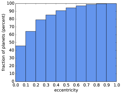
Figure 1: Cumulative histogram of orbit eccentricities of 855 exoplanets whose eccentricity were estimated; the data were retrieved from the Extrasolar Planets Encyclopedia on October 5th 2014 (Schneider,, 2014)

Multistability of the climate state further complicates estimates of the outer boundary of the HZ. Since the experience gathered with the first EBMs, it is well known that the climate of a planet can exhibit two stable states with different degree of ice-coverage (Budyko,, 1969; Sellers,, 1969), usually referred to as warm (ice-free or only partially ice-covered) and cold (completely or mostly ice-covered) climate state. Evidence suggests that Earth might have entered and exited a cold state several times in the past (Hoffman and Schrag,, 2002), and the transition to the cold state can be reproduced with state-of-the-art GCMs (Marotzke and Botzet,, 2007; Voigt and Marotzke,, 2010; Voigt et al.,, 2011). While the multistability property has been extensively discussed in the context of paleoclimate (see also Romanova et al., (2006); Yang et al., 2012a ; Yang et al., 2012b ), its implications for the habitability of exoplanets is a relatively new area of research. Lucarini et al., (2010) provided an investigation of bistability in a thermodynamic framework, which has recently been extended to include the parameters rotation rate and atmospheric opacity (Boschi et al.,, 2013; Lucarini et al.,, 2013).

The effect of obliquity and eccentricity has so far primarily been investigated with EBMs (Williams and Kasting,, 1997; Spiegel et al.,, 2009; Dressing et al.,, 2010). Their results reveal that both parameters have substantial implications for the extent of the HZ, particularly on eccentric orbits (Spiegel et al.,, 2009; Dressing et al.,, 2010). As downside of the numerical efficiency of these models, however, they rely on crude simplifications. One of their most critical simplifications is that ice is represented by simply assuming a temperature dependent surface albedo. Moreover, they do not include any dynamical processes apart from a simple diffusion parametrization of meridional heat transport. However Ferreira et al., (2014) show that the phenomenological transport efficiency relating temperature gradients and heat transport varies by an order of magnitude amongst earth-like planets at different obliquities. As these parameterizations used in EBMs for meridional heat transport are tuned to reproduce the climate of Earth, their validity is challenged by the very different shapes of atmospheric circulations and climates that can be expected on exoplanets with high polar obliquities, highly eccentric orbits, and variable degree of ice-coverage.

Despite the need for simulations with climate models of higher complexity, only three studies assessed the effect of either obliquity or eccentricity on atmospheric circulations and climate with a GCM so far (Williams and Pollard,, 2002, 2003; Ferreira et al.,, 2014). They did, however, not provide a systematic investigation of the implications for habitability. This is the aim of this work. Using a GCM of intermediate complexity we explore the atmospheric circulations and climates of idealized Earth-like planets for different astronomical parameters and examine the implications for habitability.

It is well known that silicate weathering affects the climate of Earth as a stabilizing mechanism acting on timescales of million of years: when surface temperatures are sufficiently low and rocks are not exposed to the atmosphere, the weathering is strongly suppressed, with an ensuing accumulation of CO2 in the atmosphere (Walker et al.,, 1981). In our study, we do not consider this process (see instead Williams and Kasting, (1997)) but keep the CO2 concentration at a fixed value, following Spiegel et al., (2009) and Dressing et al., (2010). Therefore, our study should be thought primarily as a parametric exploration of the effect of changing orbital parameters on a planet of given atmospheric composition rather than a realistic study of the HZ.

We anticipate that seasonal variability leads to an increase of the the maximal distance between planet and host star that allows for habitable conditions. The combined effect of obliquity and eccentricity on multistability has to our knowledge not been investigated yet. Our results reveal that obliquity is crucial in determining the extent of both the warm and cold state. Moreover, eccentric orbits are generally associated with a narrower range of two stable climate states. Our simulations also show that seasonal variability primarily leads to temporally ice-free regions, which stresses the importance of different definitions of habitability. Sensitivity experiments that include the parameters azimuthal obliquity and ocean heat capacity test the robustness of our results. Since we neglect the effect of silicate weathering, our results of the outer boundary of the habitable zone can only be used as conservative estimates. Large intra-annual variations of temperature and ice-coverage found in many of our experiments however question traditional estimates with energy balance models that do not take these variations into account.

The paper is structured as follows. In Section 2 we introduce and discuss our model PlaSim, explain the experimental setup, and list all simulations. The main features of atmospheric circulations of planets at different obliquities and eccentricities are presented in Section 3. Section 4 shows the implications of obliquity and eccentricity for multistability and the degree of habitability. A discussion of our results follows in Section 5. Finally, we draw our conclusions in Section 6.

2 Model and experimental setup

2.1 The Planet Simulator

All numerical simulations are performed with the Planet Simulator (PlaSim), a general circulation model of intermediate complexity (Fraedrich et al.,, 2005), freely available at http://www.mi.uni-hamburg.de/plasim. Atmospheric processes included in PlaSim are: atmospheric dynamics, surface turbulent fluxes, clear-sky and cloudy-sky atmosphere-radiation interaction, and moist and dry convection. The atmospheric component of the model is run coupled to a thermodynamic sea ice model and a slab ocean model (50m). The model excludes any sea ice and ocean dynamics as well as tracer chemistry and vegetation dynamics. In the following we briefly describe the parameterizations of the atmospheric component of the model that are included in the current set of numerical simulations.

• Dynamic Solver. PlaSim relies on a spectral atmospheric dynamical core to integrate the primitive equations for the vertical component of the vorticity $\zeta=\mathbf{k}\cdot(\nabla\times\mathbf{v})$ and horizontal wind divergence $\delta=\nabla_{h}\cdot\mathbf{v}$, temperature $T$ and surface pressure $p_{s}$. In spectral dynamical solvers the prognostic variables are represented as a sum of spherical harmonics truncated at order $N$ (triangular truncation is implemented in our case). Due to truncation, numerical hyperviscosity $\sim\nabla^{8}(\zeta,\delta,T)$ is applied in PlaSim to $\zeta,\delta,T$ to remove the enstrophy accumulating at the smallest resolved scales generating numerical instability.

  Sound waves are filtered by hydrostatic approximation. The Robert-Asselin time filter is used to suppress spurious computational modes associated with the leapfrog time-stepping scheme implemented to deal with the vorticity equation. More details about the numerical methods can be found in Lunkeit et al., (2011).

• Radiation. The shortwave radiation scheme is based on Lacis and Hansen, (1974) for the clear-sky atmosphere. The solar spectral range is divided into a visible and ultraviolet part $\lambda<0.75$ $\mu$ m with ozone absorption and Rayleigh scattering and a near infrared part $\lambda>0.75$ $\mu$ m with water vapor absorption only. For the cloudy fraction, transmissivities and albedos, both depending on the cloud liquid water content, are calculated differently in the near infrared and visible-ultraviolet bands, following the ideas of Stephens, (1978) and Stephens, (1984). The incoming solar flux $F_{sw}^{toa}$ at the top of the atmosphere is $F_{sw}^{toa}=S^{\star}\cos Z$, where $S^{\star}$ is the solar constant and $Z$ the zenith angle, a function of the latitude and time estimated according to Berger, (1978).

  Longwave radiation for the clear sky relies on a broad band emissivity method (e.g. Rodgers,, 1967). The transmissivities for water vapor, carbon dioxide and ozone depend on their local concentration and are determined according to the empirical relations of Sasamori, (1968). For each layer with a certain fractional cloud cover, the longwave transmissivity and cloud albedo are determined from the cloud liquid water content, the clear-sky transmissivity and the fractional cloud cover, as discussed in Slingo and Slingo, (1991). For more extensive details of the equations used to parametrize the longwave and shortwave transmissivities the reader is referred to Lunkeit et al., (2011).

  From the optical properties of the atmosphere (shortwave and longwave transmissivity and albedo), $F_{sw}^{toa}$ and the surface temperature upwards and downwards radiative fluxes at the interfaces of each atmospheric layer and hence the radiative heating rates are computed.

• Surface and moist processes. In all simulations the lower boundary is a flat surface with prescribed albedo and heat capacity. This is implemented with a shallow slab ocean model. The surface temperature therefore evolves in time according to $C_{slab}\dot{T}_{s}=F_{sw}^{surf}+F_{lw}^{-}=\sigma_{B}T_{s}^{4}+F_{sens}+F_{lat}$, where $C_{slab}$ is the heat capacity of the slab ocean, $F_{sw}^{surf}$ is the net solar radiation at the surface, $F_{lw}^{-}$ the downward longwave radiation at the surface and $F_{sens}+F_{lat}$ the sum of sensible and latent heat fluxes at the surface.

  Cumulus convection is parameterized by a Kuo-type convection scheme (Kuo,, 1965, 1974). Large scale condensation occurs when the air is supersaturated. Because condensed water is instantaneously removed as precipitation, no water is stored in clouds. Cloud cover and cloud liquid water content are diagnostic quantities. The fractional cloud cover of a grid box is parameterized following Slingo and Slingo, (1991) using the relative humidity for the stratiform cloud amount and the convective precipitation rate for the convective cloud amount. The bulk aerodynamic formulas are employed for surface flux parameterizations of wind stress ($\tau_{x},\tau_{y}$), sensible heat flux $F_{sens}$ and latent heat flux $F_{lat}$. Drag and transfer coefficients follow the approach by Louis, (1979) and Louis et al., (1981).

The thermodynamic sea ice model is based on the 0-layer version of the model of Semtner Jr, (1976), which is a simplified version of the Maykut and Untersteiner, (1971) thermodynamic sea ice model. Its main simplifications are the exclusion of the capacity of the ice to store heat and the assumption of a constant temperature gradient in the ice sheet (note that for the computation of the sea ice surface temperature a heat capacity corresponding to an ice layer with a thickness of 10 cm is assumed). Despite these simplifications, a comparison with both a more sophisticated 3-layer version of the same model and the Maykut and Untersteiner model shows deviations in the seasonal cycle of ice thickness of only about tens of centimeters (Semtner Jr,, 1976, 1984). Further simplifications of the model are the exclusion of oceanic heat transport and the exclusion of wind induced sea ice drift.

The thickness of sea ice in equilibrium is governed by thermodynamic processes (freezing and melting) and dynamic processes (advection, collision and deformation). Only thermodynamic processes are included in our model. The ice thickness is then constrained by the diffusion of heat through the ice sheet, which primarily depends on the surface temperature and oceanic heat flux. In order to avoid artificial sources of energy, the oceanic heat flux is set to zero in our model. Its limiting effect on ice growth is accounted for by prescribing a maximal ice thickness $h_{i,\rm{max}}=$3\text{\,}\mathrm{m}$$. This value is in good agreement with observation of equilibrium ice thickness between 2 and 3 m of 1-year and 2-year old sea ice on Earth (Haas,, 2009). A detailed description of the sea ice model can be found in the PlaSim reference manual (Lunkeit et al.,, 2011). A more detailed discussion of the model and also on neglecting dynamic sea ice processes can be found in Ebert and Curry, (1993).

Depending on the ice model, different processes are involved in the ice-albedo feedback. The simplest form of the feedback captures only changes in the areal extent of the ice cover. An initial perturbation of surface temperature is then amplified or damped only if it leads to a change of the the area that is ice-covered and ice-free. More realistically, also further processes associated with the ice thickness, snow cover, or melt pond characteristics can constitute positive or negative feedback mechanisms (Curry et al.,, 1995). Yet these processes require more sophisticated models and are therefore not taken into account in our experiments.

PlaSim offers a reasonable trade-off between numerical efficiency and the number of explicitly included processes. Even though all model elements have been tuned to simulate the Earth’s climate, we expect them to remain reasonably accurate for climates close to Earth’s climatic conditions. In addition to have been intensively used to study the climate of Earth, the model has already been employed in investigations of atmospheric circulations of terrestrial planets (Stenzel et al.,, 2007; Pascale et al.,, 2013), snowball transitions for different astronomical and atmospheric characteristics (Lucarini et al.,, 2013; Boschi et al.,, 2013) and the climate of tidally-locked, water-trapped planets (Menou,, 2013).

2.2 Astronomical parameters: obliquity and eccentricity

The two astronomical parameters investigated in this work are the obliquity $\theta$ of a planet (the tilt of its spin axis with respect to a normal to the plane of the orbit) ranging from $0\text{\,}\mathrm{\SIUnitSymbolDegree}$ to $90\text{\,}\mathrm{\SIUnitSymbolDegree}$ and the eccentricity $e$ of its orbit ranging from 0 to 1. Both parameters determine the temporal and spatial distribution of solar insolation (see Berger, (1978) for a comprehensive derivation of solar insolation as function of these two parameters; spatio-temporal patterns of insolation are also explored in Dobrovolskis, (2013)).

On circular orbits the spatial distribution of annual mean irradiation at the top of the atmosphere is determined by the obliquity of the planet (Figure 2). The relation between irradiation at low and high latitudes is reversed at the critical value $\theta_{c}\approx$55\text{\,}\mathrm{\SIUnitSymbolDegree}$$. For $\theta\leq\theta_{c}$, low latitudes receive on annual average more radiation than high latitudes. The converse applies for $\theta>\theta_{c}$ (Figure 2). This consequence of high obliquity has also been considered relevant for explaining geological records that hint at low-latitude glaciation in Earth’s history (Williams et al., (1998); Williams and Pollard, (2003); see also Hoffman and Schrag, (2002) for an overview), although no physical mechanism responsible for large changes of Earth’s obliquity has been found (Levrard and Laskar,, 2003; Pierrehumbert et al.,, 2011).

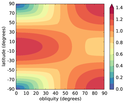
Figure 2: Annual and zonal mean irradiation at the top of the atmosphere depending on latitude and the obliquity of the planet; shown as fraction of the global average insolation $S/4$ on a circular orbit (eccentricity $e=0$)

In our experiments we set $\theta$ to $$0\text{\,}\mathrm{\SIUnitSymbolDegree}$,$60\text{\,}\mathrm{\SIUnitSymbolDegree}$$, and $90\text{\,}\mathrm{\SIUnitSymbolDegree}$, representing planets with most intensive irradiation at the equator, weak latitudinal gradients, and the highest annual mean insolation at the poles, respectively. As we aim at a parametric investigation of how different values of obliquity influence climate, we do not account for the effect of tidal processes that can erode the obliquity of a planet on time scales of billions of years (Heller et al.,, 2011).

On eccentric orbits, the insolation pattern is also influenced by the orbital longitude of periastron $\omega$ measured from northern vernal equinox (also refered to as azimuthal obliquity). This third astronomical parameter determines the hemispheric asymmetry of the annual mean insolation. Most of our analysis deals with planets with $\omega=$0\text{\,}\mathrm{\SIUnitSymbolDegree}$$, which feature an annual mean irradiation symmetric with respect to the equator. In other words, periastron and apoastron are aligned with vernal equinoxes and both hemispheres receive the same amount of energy per year. On Earth, $\omega$ changes over time, with a current value of $\omega\approx$103\text{\,}\mathrm{\SIUnitSymbolDegree}$$ (Berger,, 1978). In order to test the sensitivity of our results against changes in $\omega$, we conduct two simulations with $\omega=$30\text{\,}\mathrm{\SIUnitSymbolDegree}$$ and $\omega=$90\text{\,}\mathrm{\SIUnitSymbolDegree}$$. The latter is equivalent to an alignment of periastron with solstice, thus maximizing the difference of mean irradiation between the northern and southern hemisphere.

2.3 Experimental setup

All simulations are performed with a horizontal resolution of 64 $\times$ 32 grid points (T21 spectral resolution) and 10 vertical levels, which enables us to run a large ensemble of numerical simulations in a reasonable amount of time. In experiments not included in this paper the T21 horizontal resolution - corresponding approximately to $500$ km - has proven to provide an accurate representation of the large scale circulation features as compared to higher resolutions (T42). Most importantly, the T21 horizontal resolution captures baroclinic eddies, which play a fundamental role in the transport of energy and momentum polewards . Direct comparison between runs obtained at the two horizontal resolution T21 and T42 (not shown) demonstrate that all main features (jet streams, meridional circulation, temperature structure) are well captured at T21. Similar experiments showed that the vertical resolution ensures a convergence of the radiative transfer and an adequate representation of the vertical structure of the atmosphere.

Although the model PlaSim has been used to study the climate of planets with very different properties (see for instance Stenzel et al., (2007) for an investigation of the climate of Mars), in this work we focus on idealized planets that are Earth-like with respect to their radius, density, host star, and atmospheric composition. This choice of the setup is motivated by the presence of several studies on snowball dynamics and habitability for Earth-like planets, employing both simple EBMs (Budyko,, 1969; Sellers,, 1969; Ghil,, 1976; Bodai et al.,, 2014) and GCMs (Romanova et al.,, 2006; Marotzke and Botzet,, 2007; Voigt and Marotzke,, 2010; Voigt et al.,, 2011; Lucarini et al.,, 2010), which allows us to build on a broad basis and put our analysis in a wider context.

All planets studied in this work are completely covered with water, i.e. aquaplanets. Therefore, surface properties such as surface roughness, moisture, and heat capacity are fixed and uniform all over the globe. Also the albedo of snow- and ice-free areas is uniformly set to $\alpha=0.069$, as corresponding to an ice-free ocean. The consequences of different land-ocean distributions or different surface materials are therefore not considered in our experiments. We acknowledge that these properties might however play a crucial role in determining spatial and temporal variability and therefore interact with orbital forcing in a complex way. For instance, a planet with one large North Polar continent can experience large temperature oscillations for highly tilted spin axes due to lower heat capacity of land than ocean, potentially leading to the formation of ice caps. Spiegel et al., (2009) show that the climate of such planet indeed also shows a strong dependence on obliquity and that its habitability exhibits a much more seasonal character than on a uniform planet. A list of parameters and their chosen values can be found in Table 1.

Parameter	Symbol in text	Value(s)	Units
planet radius		6300	km
rotation rate		7.29 $\times$10-5	rad s-1
gravitational acceleration		9.81	m s-2
polar obliquity	$\theta$	{0, 60, 90}	degrees
orbit eccentricity	$e$	{0, 0.5}
azimuthal obliquity	$\omega$	⋆{0, 30, 90}	degrees
CO2 concentration		380	ppm
length of one year	$T$	360	d
length of one day		24	h
ocean albedo	$\alpha$	0.069
ocean depth	$d_{\rm{ocean}}$	⋆{10, 50}	m
ocean water density		1030	kg m-3
ocean mass specific heat capacity		4180	J kg-1 K-1
ocean horizontal diffusivity		0.0	m2 s-1
sea ice albedo		0.7
sea ice density		920	kg m-3
sea ice mass specific heat capacity		2070	J kg-1 K-1
sea ice heat conductivity		2.03	W m-1 K-1
sea ice minimal thickness		0.1	m
sea ice maximal thickness	$h_{i,\rm{max}}$	9	m

Table 1: Parameters and their values of all experiments in this study; ^⋆denotes parameters that are considered in sensitivity experiments

We modulate the intensity of the stellar irradiation $S$ that reaches the top of the atmosphere in all our simulations, which can alternatively be interpreted as changing the planet-star distance. As our model is not able to simulate the physical properties of a thick, warm atmosphere with a substantial mass fraction of H₂O, we limit our analysis to the outer edge of the HZ. Limitations of our model also imply that our definition of habitability differs from the maximum greenhouse limit that is usually considered as the outer boundary of the HZ (Kasting et al.,, 1993). Our model does not account for the effects of silicate weathering, i.e. the stabilizing feedback of CO₂ accumulation in the atmosphere, acting on timescales of millions of years, once the temperature falls sufficiently low to affect carbon fluxes at the surface. This implies that our study, in fact, should be thought primarily as a parametric exploration of the effect of changing orbital parameters on a planet of given atmospheric composition. Since we neglect a feedback pushing climate towards conditions favourable for life, we deduce that our estimated extents of the HZ are always conservative providing a lower boundary for the outer edge of the HZ. In the following, whenever we use the term habitable zone (HZ) we refer to this conservative definition of habitability. The limitations of our investigation, in particular regarding the lack of representation of the silicate weathering cycle, are later discussed in Section 5.

In the following we refer to the irradiation relative to the irradiation on Earth as $\tilde{S}=S/S^{\star}$ with $S^{\star}=$1365\text{\,}\mathrm{W}\mathrm{m}^{-2}$$. A list of all experiments whose results are presented in this work is shown in Table 2.

	Parameter values
Experiment	$e$	$\theta$	$\omega$	$d_{\rm{ocean}}$	$h_{i,\rm{max}}$
E00o00	0	$0^{\circ}$	$0^{\circ}$	50 m	3 m
E00o60	0	$60^{\circ}$	$0^{\circ}$	50 m	3 m
E00o90	0	$90^{\circ}$	$0^{\circ}$	50 m	3 m
E02o00	0.2	$0^{\circ}$	$0^{\circ}$	50 m	3 m
E02o60	0.2	$60^{\circ}$	$0^{\circ}$	50 m	3 m
E02o90	0.2	$90^{\circ}$	$0^{\circ}$	50 m	3 m
E05o00	0.5	$0^{\circ}$	$0^{\circ}$	50 m	3 m
E05o60	0.5	$60^{\circ}$	$0^{\circ}$	50 m	3 m
E05o90	0.5	$90^{\circ}$	$0^{\circ}$	50 m	3 m
E05o90om30	0.5	$90^{\circ}$	$30^{\circ}$	50 m	3 m
E05o90om90	0.5	$90^{\circ}$	$90^{\circ}$	50 m	3 m
E05o90oc10	0.5	$90^{\circ}$	$0^{\circ}$	10 m	3 m

Table 2: List of experiments and the respective values of the parameters eccentricity $e$, obliquity $\theta$, azimuthal obliquity $\omega$, ocean depth $d_{\rm{ocean}}$, and maximal sea ice thickness $h_{i,\rm{max}}$

3 Climate states and atmospheric circulations

The annual and zonal mean surface temperatures of simulations with $\theta=0^{\circ},\,60^{\circ},\,90^{\circ}$ and $e=0,\,0.5$ for ice-free climates at $S=S^{\star}$ are shown in Figure 3. Planets with low obliquities receive, on average, more stellar radiation at the equator than at the poles and usually feature a marked meridional temperature gradient. This situation is reversed at high obliquities (e.g. $\theta=90^{\circ}$) with polar regions receiving on average more radiation than equatorial regions.

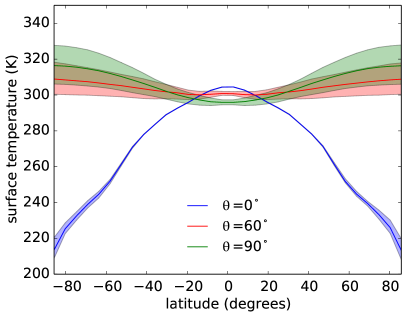
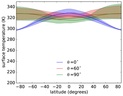
Figure 3: Annual mean, minimum and maximum surface temperature of planets with different $\theta$ and an orbit with (left) $e=0$ and (right) $e=0.5$; irradiation $S=S^{\star}$ in all experiments; (left) only the warm state (upper branch of Figure 10) is shown

Large seasonal deviations from the annual mean temperature are typical of climates at high obliquity. Patterns of zonal-mean surface temperature and zonal-mean net incoming stellar radiation are shown for each month in Fig. 4 and Fig. 5 for ice-free and snowball states for different values of obliquity and eccentricity. Because snowball states have low thermal inertia, the patterns of surface temperature follow closely the patterns of the net incoming stellar radiation. For ice-free climate states, the heat capacity of the slab ocean causes a delay of the temperature response to solar forcing of about two to three months.

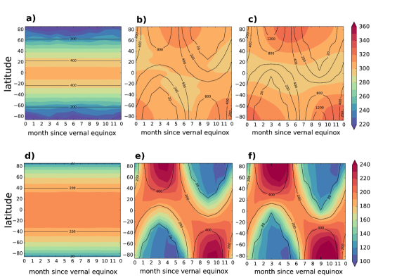
Figure 4: Annual cycle of zonal mean incoming stellar radiation (contours, W m^-2) and surface temperature (shading, K) of planets on a circular orbit ($e=0$); warm climate states (a) $\theta=0^{\circ}$, $\tilde{S}=1$, (b) $\theta=60^{\circ}$, $\tilde{S}=1$, (c) $\theta=90^{\circ}$, $\tilde{S}=1$; and snowball states ((d) $\theta=0^{\circ}$, $\tilde{S}=0.6$, (e) $\theta=60^{\circ}$, $\tilde{S}=0.6$, (f) $\theta=90^{\circ}$ , $\tilde{S}=0.6$ on a circular orbit ($e=0$)

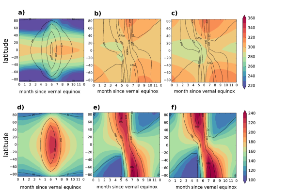
Figure 5: Annual cycle of zonal mean incoming stellar radiation (contours, W m^-2) and surface temperature (shading, K) as in Fig. 4 but of planets on an eccentric orbit with $e=0.5$; warm climate states (a) $\theta=0^{\circ}$, $\tilde{S}=0.8$, (b) $\theta=60^{\circ}$, $\tilde{S}=0.8$, (c) $\theta=90^{\circ}$, $\tilde{S}=0.8$; and snowball states ((d) $\theta=0^{\circ}$, $\tilde{S}=0.4$, (e) $\theta=60^{\circ}$, $\tilde{S}=0.4$, (f) $\theta=90^{\circ}$, $\tilde{S}=0.4$

The seasonal cycle of insolation at both high obliquity and eccentricity has a complex pattern, shifting the times of maximum insolation in the northern and southern hemisphere closer to each other (from month 3 to month 5 and from month 9 to month 7 respectively). Although solstice occurs on both poles at the same distance from the star (azimuthal obliquity $\omega=0^{\circ}$), there is a slight asymmetry in the hemispheric temperature patterns at $\theta=60^{\circ}$ and $\theta=90^{\circ}$. This is due to the fact that in the northern hemisphere summer is followed by the planet getting closer to the star, while in the southern hemisphere summer is followed by the planet moving away from the star. That is, both poles receive the same overall amount of energy, but distributed differently over time, which due to the thermal inertia gives rise to the asymmetric shape of surface temperature observed in Fig. 4 and  5.

Horizontal heat transport is essential for smoothing the effect of extreme seasonal insolation at high obliquity. Since the net incoming stellar radiation features extreme seasonal variations, also the meridional energy transport shows extreme changes over one year (Fig. 6). For planets at high obliquity (Fig. 6(a)), the mean annual transport is equatorwards at $\theta=90^{\circ}$ and nearly zero at $\theta=60^{\circ}$. During the month of maximum irradiation in the northern hemisphere (Fig. 4), the meridional heat transport is southwards at almost all latitudes, substantially differing from the annual mean values. Deviations from the annual means become extreme for frozen planets (Fig. 6(c)). Eccentricity introduces only small variations to the annual mean meridional heat transport but changes the timing of its seasonal oscillations because of shifted and distorted insolation patterns ($e=0.5$, Fig. 4(b, d)).

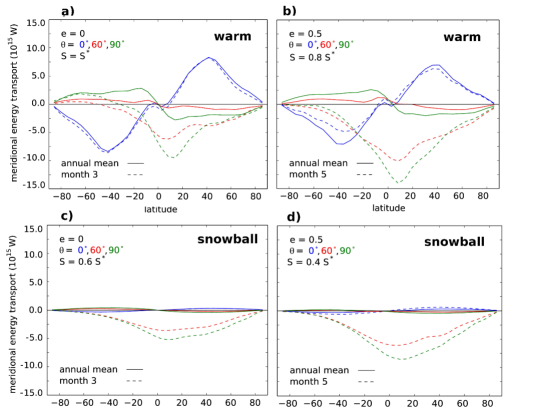
Figure 6: Total meridional transport of moist static energy for (a) a warm climate state with a circular orbit, (b) a warm climate state with an eccentric orbit, (c) a snowball state with a circular orbit, and (d) a snowball state with an eccentric orbit; each for $\theta=0^{\circ}$, $\theta=60^{\circ}$ and $\theta=90^{\circ}$; months 3 and 7 correspond to the maximal inter-hemispheric difference in incoming solar radiation

The atmospheric meridional energy transports follows directly from the atmospheric circulation. Circulations of earth-like planets with low obliquity ($\theta\rightarrow 0$) are similar to those of the Earth’s atmosphere, with equatorial regions warmer than polar regions, a direct Hadley cell confined in the Tropics and jet streams at mid-latitudes (e.g. James,, 1994). Snowball Earth-like climates for planets at low obliquity are characterized by a very dry atmosphere (neither the condensation latent heat nor the water vapor greenhouse effect have any significant impact on climate) and by very weak vertical gradients. These climates have intensively been discussed in the literature (e.g.  Pierrehumbert et al.,, 2011; Abbot et al.,, 2013; Boschi et al.,, 2013).

High obliquity causes a reversal of the atmospheric meridional temperature profile with respect to climates at low obliquity, because on annual mean equatorial regions receive more solar radiation than polar regions (Fig. 7(a, c, e, f)). In Fig. 7(a) the annual means of atmospheric temperatures and zonal winds are shown. The meridional streamfunction can be see in in Fig. 8(a) for the same temporal means. Since the circulations show pronounced seasonal variations, also the warmest month in the northern hemisphere during which there is the strongest meridional temperature contrast is included in Fig. 8.

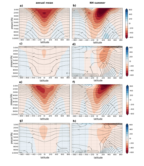
Figure 7: Annual mean (left column) and monthly mean for summer in northern hemisphere (right column) of zonal winds (m s^-1) and atmospheric temperature (K); warm states (a, b) with $\theta=90^{\circ}$, $e=0$ ($\tilde{S}=1$); snowball states (c, d) with $\theta=90^{\circ}$, $e=0$ ($\tilde{S}=0.6$); warm states (e, f) with $\theta=90^{\circ}$, $e=0.5$ ($\tilde{S}=0.8$) and snowball states (g, h) with $\theta=90^{\circ}$, $e=0.5$ ($\tilde{S}=0.4$)

Westerly storm-tracks develop in the summer hemisphere in the lower troposphere, with a strongly sheared easterly jet aloft for the warm climate at high obliquity (FIg. 7(b). The atmospheric meridional overturning circulation during the NH summer (Fig. 8(b)) is thermally direct (upwelling in the northern hemisphere and downwelling in the southern hemisphere) and extends over the whole hemisphere. The reversal of the direct cell and its shift in the southern hemisphere during the local summer results in the two small equatorial indirect cells seen in the annual mean (Fig. 8(a)), which hence are just an artefact of the annual averaging. In the winter hemisphere no strong westerly jet develops close the ground. Ferreira et al., (2014) show that the strongly sheared easterly winds in the mid-high troposphere are essential to determine baroclinic instability leading to the development of the westerly jet close to the ground, which are missing in the southern/winter hemisphere. Circulations of Earth-like planets at high obliquity and on eccentric orbits differ only slightly from the pattern discussed so far. The main difference is the asymmetric circulation between the two hemispheres (Fig. 7(e, f) and Fig. 8(e, f)) reflecting the asymmetric temperature patterns already discussed and shown in Fig. 4(c) and Fig.  5(c).

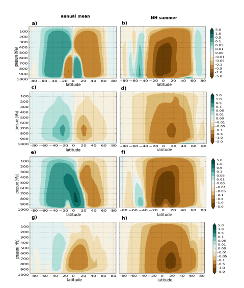
Figure 8: Annual means (left column) and northern hemisphere (right column) of the Eulerian mean stream function (in $10^{11}$  kg s^-1); warm states (a, b) with $\theta=90^{\circ}$, $e=0$ ($\tilde{S}=1$); snowball states (c, d) with $\theta=90^{\circ}$, $e=0$ ($\tilde{S}=0.6$); warm states (e, f) with $\theta=90^{\circ}$, $e=0.5$ ($\tilde{S}=0.8$); snowball states (g, h) with $\theta=90^{\circ}$, $e=0.5$ ($\tilde{S}=0.4$); the circulation goes clockwise along positive streamlines

One of main features of snowball climates is the replacement of the ocean (in our simulations represented by a slab-ocean model) with a thick ice cover, which drastically reduces the thermal inertia of the ocean. As a consequence, surface temperatures respond almost instantaneously to the distribution of absorbed solar radiation (Fig. 4,  5). As for snowball climates at low obliquity (for which a rich literature exists, (Pierrehumbert et al.,, 2011; Abbot et al.,, 2013; Boschi et al.,, 2013, e.g. )) snowball climates at high obliquity feature very weak vertical thermal gradients (Fig. 7(c, g)). This is a direct consequence of the dryness of the atmosphere and therefore the lack of greenhouse effect. Important deviations from the annually-averaged temperature profile are however observed seasonally. Fig. 7(d, h) refers to the northern hemisphere summer and shows a very stable temperature profile in the southern hemisphere, with an atmosphere which is almost isothermal, except close to the surface where a strong thermal inversion is found. The vertical profile is instead destabilized in the summer hemisphere by the intense irradiation at the ground. Air rises in the summer hemisphere forming a thermally direct cell which extends globally up to the south pole (Fig. 8(d, h)). The solstitial circulation patterns dominate the annal mean, resulting in a fictitious two-cell structure of the annually-averaged meridional streamfunction (Fig. 8(c, g)). As already noted above, changes in insolation due to eccentricity do not substantially impact the main circulation features of snowball climates at high obliquity, but introduce an asymmetric behaviour between the northern and southern hemisphere (Fig. 8(g)).

4 Multistability and habitability at extreme seasonality

Within a certain range of $\tilde{S}$, two distinct climate states coexist, one warm (mostly ice-free) and one cold (mostly ice-covered) climate state (Budyko,, 1969; Sellers,, 1969; Ghil,, 1976; Bodai et al.,, 2014). Building on previous work on the bistability and habitability of Earth-like planets (Boschi et al.,, 2013; Lucarini et al.,, 2013) the implications of seasonal variability on the stable intervals of both climate states are examined in the following. For each set of parameters, a hysteretic cycle is performed. We start the model at an irradiation around $\tilde{S}=1$ and then gradually decrease it by steps of $0.05$ until the planet is completely covered with ice. For each value of $\tilde{S}$, the model is run for fifty years, of which the last thirty years are used for the computation of climatological quantities. Once the planet is completely ice-covered, $\tilde{S}$ is step-wise increased again until the planet is completely ice-free.

4.1 Effect of obliquity on ice formation and melting

We begin our analysis by investigating the effect of obliquity on ice-formation and ice-melt on circular orbits, where the obliquity determines both the spatial distribution of insolation and its temporal variability. Our results show that both the mean distribution and its variability have substantial consequences for the transitions between the completely ice-free and the completely ice-covered climate state.

Planets with low obliquity receive most radiation at the equator, whereas planets with high obliquity receive most of their energy at the poles (Figure 2). Consequently, when decreasing $\tilde{S}$, ice formation starts at the poles and the equator for $\theta=$0\text{\,}\mathrm{\SIUnitSymbolDegree}$$ and $\theta=$90\text{\,}\mathrm{\SIUnitSymbolDegree}$$, respectively (Figure 9). This can be correlated with the spatial pattern of surface temperature (not shown) that roughly follows the distribution of annual mean insolation (Figure 2).

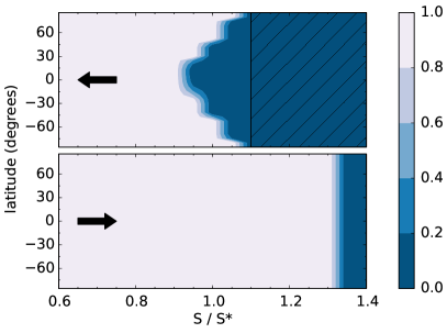
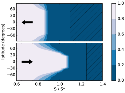
Figure 9: Ice coverage (as fraction of the year) for a planet on a circular orbit with an obliquity of $\theta=0^{\circ}$ (left) and $\theta=90^{\circ}$ (right); the zonal means of the last 10 years of each steady state are shown; the arrows indicate the direction of change of $\tilde{S}$, i.e. whether an ice-free or ice-covered initial state is assumed; hashes indicate areas outside the simulated range of $\tilde{S}$

Planets with low obliquity are more susceptible to global freezing than planets with high obliquity (Figure 9). On planets with low values of $\theta$, strong gradients of meridional temperature exist that can allow for the existence of ice at the poles despite relatively high temperatures at the equator (Figure 3). Once ice forms at the poles at a certain value of $\tilde{S}$, a further decrease of $\tilde{S}$ leads to an advancement of the ice edge towards the equator. This leads to a higher planetary albedo and thus a further cooling of the planet, which finally results in a global freezing at relatively high values of $\tilde{S}$. In contrast, temperature distributions on planets with high values of $\theta$ are more homogeneous (Figure 3). This implies that ice does not form for relatively low values of $\tilde{S}$ and hence the ice-albedo feedback does not amplify the cooling due to less incoming radiation. Yet once a critical threshold of $\tilde{S}$ is crossed and the temperature falls below the freezing point at the equator, a rather sharp transition to a completely frozen state takes place. Consequently, the transition to the completely frozen state occurs in a more gradual manner and for a higher value of $\tilde{S}$ on the planet with $\theta=$0\text{\,}\mathrm{\SIUnitSymbolDegree}$$ than for $\theta=$90\text{\,}\mathrm{\SIUnitSymbolDegree}$$ (Figure 9).

The dynamics of ice-formation and ice-melt is reversed for planets with high and low obliquity, because the geography of ice is reversed in the two cases. Melting the ice sheet of planets with $\theta=$0\text{\,}\mathrm{\SIUnitSymbolDegree}$$ requires relatively high values of $\tilde{S}$, as seasonal peak irradiation is not strong enough to trigger an initial appearance of ice-free areas at the equator. Once the critical threshold is crossed and initial ice-free areas appear, the ice-albedo feedback leads to a sharp transition. As opposed to this, planets with high values of $\theta$ feature ice-free areas at the poles already at lower values of $\tilde{S}$. Hence also the transition to a completely ice-free state occurs in a more gradual manner (Figure 9).

4.2 Effect of obliquity and eccentricity on multistability

We compute the global mean surface temperature for different values of irradiation $\tilde{S}$ in order to summarize information about the climate state into one observable. The choice of surface temperature as observable is motivated by two aspects. First, the observable can directly be linked to usual habitability conditions requiring the surface temperature to remain between the freezing and boiling point of water. Second, the observable depends strongly enough on ice-coverage to show a clear shift at the point of transition between the two distinct climate states. Also alternative ways to compress information about the climate state in one quantity based on thermodynamics have been proposed and applied in similar studies, revealing a good correlation between global mean surface temperature, material entropy production and quantities indicative of the efficiency of the climate machine (Lucarini et al.,, 2010; Boschi et al.,, 2013). However, because our focus is on average climate conditions, we choose surface temperature as observable in our analysis of climate stability. In Section 4.3 we develop a further index that is more relevant in the discussion about habitability.

In all experiments, the relationship between global mean surface temperature and solar irradiation exhibits two branches over a certain range of $\tilde{S}$. Over this range of $\tilde{S}$, the actual climate state depends on the history of the planet (Figure 10(a, b)). This phenomenon is known as climate bistability, or multistability. Where both climate states exist we distinguish them as warm and cold (snowball) climate state.

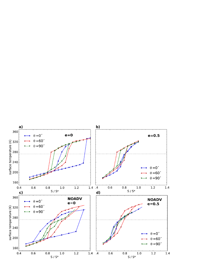
Figure 10: Annual and global mean of surface temperature versus normalized stellar irradiation for planets with obliquity $\theta=0^{\circ},60^{\circ}$ and $90^{\circ}$ and eccentricity (a) $e=0$ and (b) $e=0.5$; (c, d) hysteresis curves obtained by running the same simulations but without any horizontal transport processes (NOADV)

As explained above, the more homogeneous the distribution of surface temperature (Figure 3), the lower the critical value of $\tilde{S}$ at which the planet enters the cold state. Here, an obliquity $\theta=$60\text{\,}\mathrm{\SIUnitSymbolDegree}$$ shows the largest extent of the warm state, followed by $\theta=$90\text{\,}\mathrm{\SIUnitSymbolDegree}$$ (Figure 10(a, b)). In the cold state, ice-free areas appear once seasonal insolation at any latitude is intense enough to melt the ice cap. Therefore, the extent of the cold state is minimal for high values of obliquity (Figure 10), which are associated with very high seasonal peak irradiation.

The effect of obliquity on the extent of the warm state is qualitatively the same for a circular orbit as for an orbit with $e=0.5$. Also on such orbit, the largest extent of the warm state is shown by the planet with $\theta=60^{\circ}$, followed by $\theta=90^{\circ}$ (Figure 10(a, b)). However, the range of bistability shrinks for all experiments with $e=0.5$ compared to the experiments with $e=0$. Moreover, all experiments with $e=0.5$ show a larger extent of the warm state than the corresponding experiments with $e=0$ (Figure 10(a, b)). This can in part be explained with the increase of the global and annual mean insolation $\langle I\rangle_{e}$ on an orbit with eccentricity $e$ (Dressing et al.,, 2010), whose effect is investigated separately below:

$$\langle I\rangle_{e}=\frac{\langle I\rangle_{e=0}}{\sqrt{1-e^{2}}}.$$ (1)

Also the extent of the cold state is strongly affected by the eccentricity of the orbit. In particular for $\theta=0^{\circ}$, the width of the cold state is much smaller for $e=0.5$ than for $e=0$ (Figure 10(a, b)). This is due to the intense irradiation around periastron. While the irradiation on a planet with $\theta=0^{\circ}$ and $e=0$ is not strong enough to lead to ice-free regions, the generally higher annual mean irradiation and the high peak irradiation around periastron on an orbit with $e=0.5$ suffice to melt the ice layer. This generally leads to a sharper transition between the two states and possibly only one stable state for higher eccentricities (Figure 10(a, b)). This bifurcation from two stable states to only one stable state was also observed in previous studies where the length of one year was varied (Lucarini et al.,, 2013).

Meridional transport processes due to atmospheric dynamics play a crucial role in determining the behaviour of the ice-albedo feedback and therefore also affect the transitions between ice-free and ice-covered climate states. Hysteresis curves shown in Fig. 10(c, d) are obtained after “switching off” the atmospheric dynamic core of PlaSim, leaving each atmospheric column isolated from its neighbouring columns and in radiative-convective equilibrium. Because temperature differences are not smoothed by transport processes, large gradients build up between regions with more and less intense insolation. These simulations show that the absence of horizontal transport processes has as a consequence for the disappearance of the catastrophic events in the hysteresis curves. For different obliquities and different eccentricities the planets get gradually frozen without the sudden glaciation observed in full-dynamics simulations (Fig. 10(c, d)). This is in line with the analysis of results obtained from one-dimensional EBM of Earth, showing that the sensitivity of the ice-line to changes in solar radiation, which goes to infinity during a snowball catastrophe, is identically zero if there is no meridional heat transport (Roe and Baker,, 2010). As concluding remark we note that, although catastrophic events represented by sudden jumps of the mean surface temperature disappear when transport processes are excluded, hysteresis still remains with curves showing characteristics different between the two directions of the transition.

4.3 Implications for habitability

The existence of liquid water is the most common criterion for habitability. In estimates of the outer boundary of the habitable zone with zero dimensional EBMs or RCMs, this has been translated to the requirement of a global average surface temperature above the freezing point of water. Another sufficient condition for habitability is the existence of a warm stable climate state, because in the case of bistability the warm state always features some ice-free areas. These two conditions are however conservative and neglect that in case of spatial and temporal heterogeneity ice-free areas can also exist under both conditions, at a global mean surface temperature below the freezing point and in a cold climate state.

We therefore use a slightly modified version of the definition of temporal habitability proposed by Spiegel et al., (2008), based on sea ice cover instead of surface temperature as measure for habitability. This reflects our use of an explicit sea ice model and the fact that stability issues of PlaSim do not allow to simulate climate close to the boiling point of water, which restricts our analysis to the outer boundary of the HZ. We then compute the zonal habitability $H(\varphi,t)$ from sea ice cover $\sigma(\varphi,\lambda,t)$ according to

$$H(\varphi,t)=1-\frac{1}{2\pi}\int_{0}^{2\pi}\sigma(\varphi,\lambda,t)\rm{d}\lambda,$$ (2)

where $\varphi$ and $\lambda$ are latitude and longitude respectively. The temporal habitability $f(\varphi)$ is then defined as

$$f(\varphi)\;=\;\frac{\int_{t=0}^{T}\;H(\varphi,t)\;dt}{T}$$ (3)

where $T$ denotes the length of one year. We then classify each climate state as one of the following:

• habitable if $f(\varphi)=1$ at all latitudes $\varphi$

• partially habitable if $f(\varphi)=1$ at some latitude

• temporally habitable if $f(\varphi)>0$ at some latitude but $f(\varphi)<1$ at all latitudes

• unhabitable if $f(\varphi)=0$ at all latitudes

Our experiments reveal several aspects of the effect of obliquity and eccentricity on a planet’s habitability. First of all, seasonal variability can lead to a substantial extension of the habitable zone. While a planet with $e=0$ and $\theta=0^{\circ}$ is habitable for $\tilde{S}>0.95$ (warm initial state) or $\tilde{S}>1.3$ (cold initial state), a planet with $e=0.5$ and $\theta=90^{\circ}$ is habitable for $\tilde{S}>0.55$ (E05o90, Figure 11). Moreover, also cold climate states can exhibit regions that are temporally and even continously ice free. While the extent of the warm state is an appropriate measure of the HZ on planets without seasonal variations (E00o00, Figure 11), it leads to a substantial underestimation of the HZ on planets with large seasonal variations (E05o90, Figure 11).

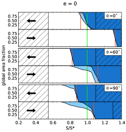
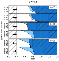
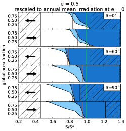
Figure 11: Degree of habitability for simulations with $e=0$ (left) and $e=0.5$ (center), and $\theta=0,60,90^{\circ}$ (from top to bottom); the color denotes the fraction of the planet’s surface that is (partially) habitable (dark blue), temporally habitable (light blue) and unhabitable (white); the red vertical line marks the point of transition between the warm and cold state; the solid green vertical line shows the solar irradiation at $1\text{\,}\mathrm{A}\mathrm{U}$ as reference; (right) results for $e=0.5$ rescaled according to the annual mean irradiation $\langle I\rangle_{e=0.5}$ (see Equation 1), such that the total annual amount of energy received from the star is the same as for $e=0$ (left); the arrows indicate the direction of change of $\tilde{S}$, i.e. whether an ice-free or ice-covered initial state is assumed; hashes indicate areas outside the simulated range of $\tilde{S}$

On such planets the extension of the HZ is mainly due to regions that are temporally habitable, i.e ice free only at some time of the year. A clear distinction between partial and temporal habitability is therefore not only motivated from a biological perspective but also strongly suggested by the results of our climate simulations. Because eccentricity affects both the annual mean irradiation and its variability, these two effects have to be analysed separately. This is illustrated in the right column of Figure 11. Here the results of the simulations at $e=0.5$ are rescaled to the mean irradiation at $e=0$ by dividing them through the factor at which the annual mean irradiation increases from $e=0$ to $e=0.5$ (see Equation 2). The results show that while the increase of annual mean irradiation with eccentricity is a good proxy for the extent of the warm state on an eccentric orbit, the simple scaling does neither capture the effects that lead to the extension of the HZ nor the effects that limit the extent of the cold state on an eccentric orbit. The remaining effect of eccentricity has to be attributed to the higher amplitude of the seasonal cycle and the different spatial and temporal distribution of irradiation (Figure 11).

Whether temporally habitable regions might indeed be suitable for life might depend on the amplitude of these seasonal variations and how long such regions might be ice-covered and ice-free. The presence of land masses (not accounted for in this study) may in turn facilitate or go against this partially habitable, ice-free regions. As illustrative examples we show the seasonal cycle of surface temperature and ice thickness of two simulations on an orbit with $e=0.5$ and $\theta=0^{\circ}$ and $\theta=90^{\circ}$. Both are shown for $\tilde{S}=0.7$ (Figure 12 and 13). The planet with $\theta=0^{\circ}$ shows largest seasonal variations at low latitudes. Here surface temperatures exceed the freezing point for a short period around periastron, but long enough for a tiny area to become temporally ice free (Figure 12).

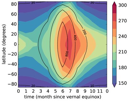
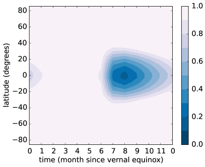
Figure 12: Seasonal cycle of surface temperature (K; colors, left), irradiation $S$ (W/m²; lines, left), and sea ice thickness ($h_{i}~{}/h_{i,\rm{max}}$; right) of the experiment E05o00 at $\tilde{S}=0.7$ ($S=$956\text{\,}\mathrm{W}\mathrm{m}^{-2}$$)

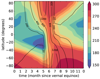
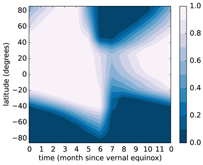
Figure 13: Seasonal cycle of surface temperature (K; colors, left), irradiation $S$ (W/m²; lines, left), and sea ice thickness ($h_{i}~{}/h_{i,\rm{max}}$; right) of the experiment E05o90 at $\tilde{S}=0.7$ ($S=$956\text{\,}\mathrm{W}\mathrm{m}^{-2}$$); note that the temporal evolution of $S$ differs among the two hemispheres due to the eccentric orbit, leading to an asymmetric distribution of surface temperature and ice-thickness

As compared to this, the climate of the planet with $\theta=90^{\circ}$ is extremely variable, with almost half of the planet’s surface experiencing freezing and complete melting in one year (Figure 13). Also surface temperatures show considerable oscillations with a maximal amplitude of the annual cylce of about 100 K at the equator. Apart from these unhabitable regions, however, high latitudes around the South Pole show rather moderate climatic conditions with a temperature oscillation of only about 20 K (Figure 13).

The experiments shown in Figure 12 and Figure 13 differ only in the polar obliquity $\theta$. As both planets exhibit ice-free areas at some point of the year, they are equally classified as temporally habitable for $\tilde{S}=0.7$. Yet a closer look reveals substantial differences with respect to the size of the temporally habitable area, the time this area is ice-free, and the amplitude of surface temperature at that location. Although the total amount of energy per year that both planets receive is the same, its different temporal and spatial distribution leads to extremely different climatic conditions.

4.4 Sensitivity to asymmetric mean irradiation and heat capacity

In all numerical experiments with eccentric orbits we assumed that the total radiation received over one year is symmetrically distributed among the two hemispheres ($\omega=0^{\circ}$). Our results show, however that the expansion of the HZ due to seasonal variability is primarily determined by the peak of the locally incoming radiation and whether this maximal radiation suffices to lead to temporally ice-free regions. We therefore expect that an uneven distribution of mean radiation and a higher peak radiation at one pole, both associated with $\omega\neq 0^{\circ}$, leads to a further extension of the HZ. In order to quantify this effect, we consider the most extreme case $\omega=90^{\circ}$ (solstice aligned with periastron). In a previous study (Dressing et al.,, 2010) experiments with $\omega=30^{\circ}$ showed the maximal extent of the HZ. We also include one simulation with $\omega=30^{\circ}$, although we expect that the value of $\omega$ associated with the maximal expansion of the HZ is sensitive to further parameters such as the planet’s heat capacity.

The results are shown in Figure 14. As a consequence of the very warm polar summer for $\omega=$90\text{\,}\mathrm{\SIUnitSymbolDegree}$$, high latitudes becomes ice-free out to $\tilde{S}>0.35$. Moreover, as the incoming radiation is less evenly distributed, the temporally ice-free areas shrink compared to $\omega=0^{\circ}$. In contrast to Dressing et al., (2010), our experiments show the maximal expansion of the HZ for $\omega=$90\text{\,}\mathrm{\SIUnitSymbolDegree}$$ (Figure 14). We conclude that an uneven irradiation with $\omega=$90\text{\,}\mathrm{\SIUnitSymbolDegree}$$ leads to the most extreme climates in our experiments with small areas becoming temporary ice-free for even very low values of $\tilde{S}$.

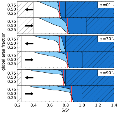
Figure 14: Degree of habitability as in Figure 11, here for $e=0.5$, $\theta=$90\text{\,}\mathrm{\SIUnitSymbolDegree}$$, and $\omega=0,30,$90\text{\,}\mathrm{\SIUnitSymbolDegree}$$; the arrows indicate the direction of change of $\tilde{S}$, i.e. whether an ice-free or ice-covered initial state is assumed; the red vertical line marks the point of transition between the warm and cold state; hashes indicate areas outside the simulated range of $\tilde{S}$

Variations of surface temperature due to seasonal forcing are damped by the heat capacity of the planet. The mean value and the amplitude of surface temperature at $e=0.5$ and $\theta=0^{\circ}$ and $\theta=90^{\circ}$ are depicted in Figure 15. Both experiments show roughly the same pattern. In an ice-free state, temperature oscillations are relatively small ($\sim$ 10-20 K, Figure 15). With sea ice at the surface, this amplitude increases up to more than 100 K as the exchange of heat between the atmosphere and ocean is reduced and the ice-albedo feedback further amplifies temperature variations (Figure 15).

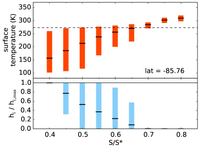
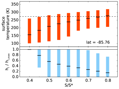
Figure 15: Annual mean, maximum and minimum of surface temperature and normalized sea ice thickness ($h_{i,\rm{max}}=$3\text{\,}\mathrm{m}$$, indicated by the black horizontal line) of the experiments E05o90 with an ocean depth of 50 m (left) and E05o90oc10 (right) with an ocean depth set to 10 m (left)

Choosing an ocean depth of 10 m in our sensitivity experiment hence affects the temperature oscillations and ice coverage only in warm climate states (Figure 15). In addition, lower heat capacity leads to the formation of ice at higher irradiation $\tilde{S}$, as less heat can be stored around periastron and the surface temperature thus drops below the freezing point around apoastron. Hence, although a reduced heat capacity reduces the continuously habitable surface area in favor of temporally habitable regions, it has no effect on the lower limit of $\tilde{S}$ that still leads to ice-free areas. The sensitivity experiment thus demonstrates that our estimate of the HZ is robust with respect to changing the heat capacity of the surface layer.

5 Discussion

In this work we provide for the first time a parametric investigation of the effect of seasonal variability on the climate of idealized Earth-like planets based on a general circulation model (GCM), having in mind the exploration of habitability conditions. Exploring the effects of the two parameters obliquity and eccentricity we build on previous work with energy balance models (EBMs) that focuses on the same parameters but in which simpler models are used (Spiegel et al.,, 2009; Dressing et al.,, 2010). At the same time our work complements parametric investigations with the same model focusing on different parameters (Boschi et al.,, 2013; Lucarini et al.,, 2013). Although the realism of our experiments regarding the determination of the HZ is constrained by both neglecting the silicate weathering cycle and the lack of a dynamic ocean and a dynamic sea ice model, we aim to provide valuable insights into the effects of seasonal variability for the climate of idealized planets on shorter time scales.

The numerical experiments performed in this work are based on the assumption of idealized aquaplanets. In order to test the robustness of our results further aspects need to be taken into account. First, our idealized planets are all characterized by uniform surface characteristics. As discussed in Section 2.3, surface heat capacity, albedo, and moisture supply can alter externally induced temperature oscillations and substantially affect the atmospheric dynamics of a planet. The effects of different land-sea distributions are taken into account in Williams and Pollard, (2003) and Spiegel et al., (2009), but a detailed investigation with general circulation models has not been done yet.

Second, our numerical experiments are performed with a slab ocean model and thus do not account for oceanic heat transport. On tidally locked planets, where strong spatial variations can imply spatially confined habitable conditions similar to our results (Pierrehumbert,, 2011), oceanic heat transport can lead to a substantial extension of the HZ (Hu and Yang,, 2014). However, for high obliquity and low eccentricity Ferreira et al., (2014) demonstrated that slab ocean models reproduce well the surface climate of coupled simulations for an ocean depth of 50 m.

Third, only thermodynamic sea ice processes are represented in our model. Any dynamical processes such as wind induced sea ice drift or the flow of sea ice due to gravity are not taken into account. In some cases we expect this to limit the realism of our results. In the experiment of a planet on an eccentric orbit with $\theta=$0\text{\,}\mathrm{\SIUnitSymbolDegree}$$, for instance, the prescribed maximal sea ice thickness might bias our results towards temporally habitable conditions, because sea ice is not allowed to grow beyond a thickness of $3\text{\,}\mathrm{m}$ anywhere on the planet during apoastron. Without this restriction, sea ice could grow much thicker at the poles and subsequently flow towards lower latitudes, preventing the quick melt of the sea ice layer that appears in our simulation and thus resulting in a permanently unhabitable climate. Taking Earth as reference, a sea ice thickness beyond 3 m might indeed be realistic on exoplanets, as it is estimated that during Snowball events Earth was covered by an ice layer several hundreds of meters thick (Abbot et al.,, 2010; Pierrehumbert et al.,, 2011). A further limitation of our sea ice model might be due to a too high amplitude of the seasonal cycle of surface temperatures, attributable to the low vertical resolution of the ice layer in our model (Abbot et al.,, 2010). Because associated high peak values of surface temperature are required for the existence of ice-free areas in some of our simulations, also this limitation of our sea ice model tends to bias our results towards (temporally) habitable conditions.

Fourth, the effect of a different rotation rate needs to be investigated because of its large impact on the meridional heat transport (Vallis and Farneti,, 2009). Experiments with energy balance models where the effect of the planetary spin rate is parametrized through the meridional heat transport diffusion coefficient show that on planets with seasonal variability, the effect on habitability is comparatively small (Spiegel et al.,, 2009; Dressing et al.,, 2010). Besides its effect on the meridional transport of energy, the planetary spin also affects climate through diurnal variability, which may have a large effect on habitability for slowly rotating and phase-locked planets.

Several authors have addressed the effect of seasonal variability on the habitability of exoplanets using climate models of lower complexity. On circular orbits, our results are in good agreement with previous results based on one-dimensional latitudinal resolved EBMs (Spiegel et al., (2009), Figure 16). They also agree well in a qualitative sense with recent work based on an energy balance model (Armstrong et al.,, 2014), showing a positive relation between obliquity and the maximal habitable zone. On eccentric orbits with $e=0.5$, however, simulations with EBMs tend to overestimate the outer boundary of the HZ relative to our results (Dressing et al., (2010), Figure 16). Despite this overestimation, the qualitative effect of obliquity agrees well also on eccentric orbits, showing the maximal extent for planets with $\theta=90^{\circ}$ (Figure 16).

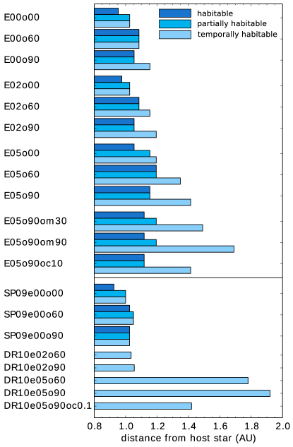
Figure 16: Maximal distance between planet and host star that allows for habitable, partially habitable and temporally habitable climate conditions; the results of the last eight experiments denoted by SP09 and DR10 are taken from Spiegel et al., (2009) and Dressing et al., (2010) respectively; both use the same EBM and simulate the climate of Earth-like planets on circular (SP09) and eccentric orbits (DR10); while in both studies an ocean surface fraction of 70 % is default, this fraction is set to 10 % in the simulation DR10e05o90oc0.1

Conversely to the overestimation of the HZ by EBMs at $e=0.5$, simulations at $e=0.2$ show a smaller extent of the HZ simulated by EBMs than observed in our experiments (Figure 16). This somewhat surprising observation might be attributable to slightly different experimental setups of the EBMs used in the experiments at $e=0$ and $e=0.2$ (Spiegel et al.,, 2009; Dressing et al.,, 2010), but can also hint at a non-linear effect of eccentricity on the extent of the HZ in the EBMs. Such effect might originate from the complex interplay between the different timescales of variability, which is dramatically simplified by assessing only its consequence for the extent of the HZ.

Apart from apparent differences between the two different classes of models, such as the explicit simulation of the atmospheric circulation in our model, further explanations for the discrepancies are different definitions of habitability and the representation of ice processes. While Spiegel et al., (2008) and subsequent studies use $T_{s}\geq$273\text{\,}\mathrm{K}$$ as condition for habitability, our definition is based on ice-coverage of the surface. Hence it suffices that the surface temperature shortly exceeds the melting point to be habitable in their model, while in our experiments it is required that the sea ice be locally completely melted. This difference becomes more severe due to the representation of the ice-albedo feedback in the two models. While the sea ice model of PlaSim considers only the areal extent of sea ice, i.e. a complete melting of the ice column is required to affect the surface albedo and therefore amplify the initial signal, the EBM incorporates a smooth dependency of surface albedo on temperature, which can be interpreted as the inclusion of melting ponds on top of the ice sheet and facilitates numerical computations.

The most critical limitations of our work are shared with these previous studies. These limitations are due to the neglection of the effect of CO₂ accumulation on the extent of the HZ. The most common estimates of the habitable zone rely on zero dimensional radiation convection models (RCMs). As opposed to our general circulation model, these models include feedback mechanisms of the carbon cycle: on the one hand, a decrease of surface temperature reduces the rate of chemical weathering at the surface, which leads to an accumulation of CO₂ in the atmosphere and an enhanced greenhouse effect. On the other hand, a higher concentration of CO₂ leads to an increased Rayleigh scattering of incoming radiation, which tends to further decrease the surface temperature. The outer boundary of the HZ, also called the maximum greenhouse limit, is then defined by the balance between these two processes (Kasting et al.,, 1993). Because our aim is a parametric investigation of the effects of obliquity and eccentricity on habitability, we have to limit the number of parameters and our experiments can not provide a realistic estimate of habitability of a generic planet. In leaving aside the stabilizing effect of silicate weathering, however, we provide conservative estimates of the HZ.

6 Conclusions

Our results show a great diversity of climates due to different obliquities and orbit eccentricities. Moreover, seasonal variability has a large effect on habitability. For planets with Earth-like atmospheres, seasonal variability can extend the maximal distance between planet and host star that still allows for habitable conditions from $1.03\text{\,}\mathrm{A}\mathrm{U}$ (obliquity $\theta=0^{\circ}$, eccentricity $e=0$) to $1.69\text{\,}\mathrm{A}\mathrm{U}$ ($\theta=90^{\circ}$, $e=0.5$, $\omega=90^{\circ}$). While the effect of obliquity on habitability is comparatively small on circular orbits, it becomes highly relevant on eccentric orbits. This effect of seasonal variability on habitability is primarily due to regions that are ice-free only at some time of the year. An appropriate assessment of the HZ therefore asks for a clear distinction between different degrees of habitability (Table 3).

	Maximal distance from host star
Experiment	Habitable	Partially habitable	Temporally habitable
E00o00	0.95 AU	1.03 AU	1.03 AU
E00o60	1.08 AU	1.08 AU	1.08 AU
E00o90	1.05 AU	1.05 AU	1.15 AU
E02o00	0.98 AU	1.03 AU	1.03 AU
E02o60	1.08 AU	1.08 AU	1.15 AU
E02o90	1.05 AU	1.05 AU	1.20 AU
E05o00	1.05 AU	1.15 AU	1.20 AU
E05o60	1.20 AU	1.20 AU	1.35 AU
E05o90	1.15 AU	1.15 AU	1.41 AU
E05o90om30	1.12 AU	1.20 AU	1.49 AU
E05o90om90	1.12 AU	1.20 AU	1.69 AU
E05o90oc10	1.12 AU	1.12 AU	1.41 AU

Table 3: Maximal distance between planet and host star that allows for habitable, partially habitable, and temporally habitable climatic conditions

Moreover, our experiments show that the multistability of the climate state is strongly influenced by the obliquity of a planet, in particular on circular orbits. The largest extent of the warm state is found for an obliquity around $\theta=$55\text{\,}\mathrm{\SIUnitSymbolDegree}$$, where the temperature distribution is most homogeneous. The smallest extent of the warm state and the largest extent of the cold state is found for planets with low values of obliquity. On eccentric orbits, the range of distances that allow for two stable climate states shrinks relative to circular orbits, possibly leading to monostability for planets with very large seasonal variability. While the extent of the warm climate state is a good proxy for the habitability of planets without seasonal variability, this does not hold for planets with high obliquities and on eccentric orbits, since also cold states can allow for ice-free regions. Whether life can exist in such extreme climates with strong temporal and spatial variability in surface conditions is still an open question (Kane and Gelino,, 2012). Our results also suggest a need for more sophisticated indicators of climate that account for the effects of strong variability.

Some of the effects of seasonal variability can be attributed to an increase of the annual mean irradiation with eccentricity. Nonetheless, while this effect of eccentricity can in part explain the extension of the warm state on eccentric orbits, it does neither capture the widening effect on the HZ nor the limiting effect on the extent of the cold state.

Estimates of the outer boundary of the HZ that are based on RCMs and account for silicate weathering yield a maximal planet-star distance of $1.67\text{\,}\mathrm{A}\mathrm{U}$ (Kasting et al.,, 1993), recently updated to $1.70\text{\,}\mathrm{A}\mathrm{U}$ (Kopparapu et al.,, 2013). These estimates, however, rely on the assumption of a constant and uniform surface temperature, which is - as show in our results - a crude simplification of the problem. Planets with high seasonal variability can indeed feature a mean surface temperature below 240 K although having large areas completely ice-free throughout the year (Figure 8). How weathering might be affected by such a high spatial and temporal variability and what this implies for estimates of the outer boundary of the habitable zone is an interesting open question. Future investigations with GCMs that combine seasonal variability, a dynamic CO₂ concentration, and ocean and sea ice dynamics are required in order to provide further insights into the implications of seasonal variability for the climate of exoplanets and their ability to host life.

References

- Abbot et al., (2010) Abbot, D. S., Eisenman, I., and Pierrehumbert, R.T. (2010). The Importance of Ice Resolution for Snowball Climate and Deglaciation. J. Climate, 23(22):6100 –6109.
- Abbot et al., (2013) Abbot, D. S., Voigt, A., Li, D., Le Hir, G., Pierrehumbert, R. T., Branson, M., Pollard, D., and Koll, D. D. B. (2013). Robust elements of Snowball Earth atmospheric circulation and oases for life. Journal of Geophysical Research, 118:6017 – 6127.
- Armstrong et al., (2014) Armstrong, J. C., Barnes, R., Domagal-Goldman, S., Breiner, J., Quinn, T. R., and Meadows, V. S. (2014). Effects of extreme obliquity variations on the habitability of exoplanets.. Astrobiology, 14(4):277–291.
- Berger, (1978) Berger, A. (1978). Long-term variations of daily insolation and quaternary climatic changes. J. Atmos. Sci., 35(12):2362–2367.
- Bodai et al., (2014) Bodai, T., Lucarini, V., Lunkeit, F., and Boschi, R. (2014). Global instability in the Ghil–Sellers model. Climate Dynamics, ISSN 0930-7575:1–21.
- Borucki et al., (2011) Borucki, W. J., Koch, D. G., Basri, G., Batalha, N., Brown, T. M., Bryson, S. T., Caldwell, D., Christensen-Dalsgaard, J., Cochran, W. D., DeVore, E., et al. (2011). Characteristics of planetary candidates observed by Kepler. II. Analysis of the first four months of data. The Astrophysical Journal, 736(1):19.
- Boschi et al., (2013) Boschi, R., Lucarini, V., and Pascale, S. (2013). Bistability of the climate around the habitable zone: a thermodynamic investigation. Icarus, 226(2):1724–1742.
- Budyko, (1969) Budyko, M. I. (1969). The effect of solar radiation variations on the climate of the earth. Tellus, 21:611–619.
- Curry et al., (1995) Curry, J. A., Schramm, J. L., and Ebert, E. E. (1995). Sea ice-albedo climate feedback mechanism. Journal of Climate, 8(2):240–247.
- Dobrovolskis, (2013) Dobrovolskis, A. R. (2013). Insolation on exoplanets with eccentricity and obliquity. Icarus, 226(1):760 – 776.
- Dressing et al., (2010) Dressing, C. D., Spiegel, D. S., Scharf, C. A., Menou, K., and Raymond, S. N. (2010). Habitable climates: The influence of eccentricity. The Astrophysical Journal, 721(2):1295.
- Eady, (1949) Eady, E. (1949). Long waves and cyclone waves. Tellus, 1:33 – 52.
- Ebert and Curry, (1993) Ebert, E. E. and Curry, J. A. (1993). An intermediate one-dimensional thermodynamic sea ice model for investigating ice-atmosphere interactions. Journal of Geophysical Research: Oceans (1978–2012), 98(C6):10085–10109.
- Ferreira et al., (2014) Ferreira, D., Marshall, J., O’Gorman, P. A., Seager, S. (2014). Climate at high-obliquity. Icarus, 243:236–-248.
- Ford et al., (2008) Ford, E. B., Quinn, S. N., and Veras, D. (2008). Characterizing the orbital eccentricities of transiting extrasolar planets with photometric observations. The Astrophysical Journal, 678:1407–1418.
- Fraedrich et al., (2005) Fraedrich, K., Jansen, H., Kirk, E., Luksch, U., and Lunkeit, F. (2005). The planet simulator: Towards a user friendly model. Meteorologische Zeitschrift, 14(3):299–304.
- Ghil, (1976) Ghil, M. (1976). Climate stability for a Sellers-type model. Journal of the Atmospheric Sciences, 33(1):3–22.
- Haas, (2009) Haas, C. (2009). Sea Ice: An Introduction to its Physics, Chemistry, Biology and Geology, chapter 4: Dynamics versus thermodynamics: The sea ice thickness distribution, pages 113–151. Wiley-Blackwell.
- Hart, (1979) Hart, M. H. (1979). Habitable Zones about Main Sequence Stars. Icarus, 37:351–357.
- Heller et al., (2011) Heller, R., Leconte, J., and Barnes, R. (2011). Tidal obliquity evolution of potentially habitable planets. Astronomy and Astrophysics, 528:27.
- (21) Heng, K., Menou, K., and Phillipps, P. J. (2011). Atmospheric circulation of tidally locked exoplanets: a suite of benchmark tests for dynamical solvers. MNRAS , 413:2380.
- (22) Heng, K., Frierson, D. M. W., and Phillipps, P. J. (2011). Atmospheric circulation of tidally locked exoplanets: II Dual-band radiative transfer and convective adjustment. MNRAS , 418(4):2669.
- Hoffman and Schrag, (2002) Hoffman, P. F. and Schrag, D. P. (2002). The snowball earth hypothesis: testing the limits of global change. Terra Nova, 14(3):129–155.
- Howard, (2013) Howard, A. W. (2013). Observed properties of extrasolar planets. Science, 340(6132):572–576.
- Hu and Yang, (2014) Hu, Y. and Yang, J. (2014). Role of ocean heat transport in climates of tidally locked exoplanets around m dwarf stars. Proceedings of the National Academy of Sciences, 111(2):629–634.
- James, (1994) James, I. N. (1994). Introduction to Circulating Atmosphere, 448 pp. Cambridge University Press.
- Kane et al., (2012) Kane, S. R., Ciardi, D. R., Gelino, D. M., and von Braun, K. (2012). The exoplanet eccentricity distribution from Kepler planet candidates. Monthly Notices of the Royal Astronomical Society, 425:757–762.
- Kane and Gelino, (2012) Kane, S. R. and Gelino, D. M. (2012). The Habitable Zone and extreme planetary orbits. Astrobiology, 12:940–945.
- Kasting et al., (1993) Kasting, J. F., Whitmire, D. P., and Reynolds, R. T. (1993). Habitable zones around main sequence stars. Icarus, 101:108–128.
- Kopparapu et al., (2013) Kopparapu, R. K., Ramirez, R., Kasting, J. F., Eymet, V., Robinson, T. D., Mahadevan, S., Terrien, R. C., Domagal-Goldman, S., Meadows, V., and Deshpande, R. (2013). Habitable zones around main-sequence stars: New estimates. The Astrophysical Journal, 765:131.
- Kuo, (1965) Kuo, H.-L. (1965). On formation and intensification of tropical cyclones through latent heat release by cumulus convection. Journal of the Atmospheric Sciences, 22(1):40–63.
- Kuo, (1974) Kuo, H.-L. (1974). Further studies of the parameterization of the influence of cumulus convection on large-scale flow. Journal of the Atmospheric Sciences, 31(5):1232–1240.
- Lacis and Hansen, (1974) Lacis, A. A. and Hansen, J. (1974). A parameterization for the absorption of solar radiation in the earth’s atmosphere. Journal of the Atmospheric Sciences, 31(1):118–133.
- Leconte et al., (2013) Leconte, J., Forget, F., Charnay, B., Wordsworth, R., Selsis, F., Millour, E., and Spiga, A. (2013). 3d climate modeling of close-in land planets: Circulation patterns, climate moist bistability, and habitability. Astronomy and Astrophysics, 554:69.
- Levrard and Laskar, (2003) Levrard, B. and Laskar, J. (2003). Climate friction and the Earth’s obliquity. Geophysical Journal International, 154:970–990.
- Louis et al., (1981) Louis, J., Tiedke, M., and Geleyn, M. (1981). A short history of the PBL parameterisation at ECMWF, page 59–80.
- Louis, (1979) Louis, J.-F. (1979). A parametric model of vertical eddy fluxes in the atmosphere. Boundary-Layer Meteorology, 17(2):187–202.
- Lucarini et al., (2010) Lucarini, V., Fraedrich, K., and Lunkeit, F. (2010). Thermodynamic analysis of snowball earth hysteresis experiment: efficiency, entropy production and irreversibility. Quarterly Journal of the Royal Meteorological Society, 136(646):2–11.
- Lucarini et al., (2013) Lucarini, V., Pascale, S., Boschi, R., Kirk, E., and Iro, N. (2013). Habitability and multistability of Earth-like planets. Astronomische Nachrichten, 334:576–588.
- Lunkeit et al., (2011) Lunkeit, F., Fraedrich, K., Jansen, H., Kirk, E., Kleidon, A., and Luksch, U. (2011). Planet Simulator reference manual, available at http://www.mi.uni-hamburg.de/plasim.
- Marotzke and Botzet, (2007) Marotzke, J. and Botzet, M. (2007). Present-day and ice-covered equilibrium states in a comprehensive climate model. Geophysical Research Letters, 34(16):L16704.
- Maykut and Untersteiner, (1971) Maykut, G. A. and Untersteiner, N. (1971). Some results from a time-dependent thermodynamic model of sea ice. Journal of Geophysical Research, 76(6):1550–1575.
- Menou, (2012) Menou, K. (2012). Atmospheric circulation and composition of GJ1214b. The Astrophysical Journal Letters, 744:L16.
- Menou, (2013) Menou, K. (2013). Water-trapped worlds. The Astrophysical Journal, 774:51–2367.
- Merlis and Schneider, (2010) Merlis, T. M. and Schneider, T. (2010). Atmospheric Dynamics of Earth-Like Tidally Locked Aquaplanets. J. Adv. Model. Earth Syst., 2, 13.
- Moorhead et al., (2011) Moorhead, A. V., Ford, E. B., Morehead, R. C., Rowe, J., Borucki, W. J., Batalha, N. M., Bryson, S. T., Caldwell, D. A., Fabrycky, D. C., Gautier, III, T. N., Koch, D. G., Holman, M. J., Jenkins, J. M., Li, J., Lissauer, J. J., Lucas, P., Marcy, G. W., Quinn, S. N., Quintana, E., Ragozzine, D., Shporer, A., Still, M., and Torres, G. (2011). The distribution of transit durations for Kepler planet candidates and Implications for Their Orbital Eccentricities. The Astrophysical Journal Supplement Series, 197:1 (15pp).
- Pascale et al., (2013) Pascale, S., Ragone, F., Lucarini, V., Wang, Y., and Boschi, R. (2013). Nonequilibrium thermodynamics of circulation regimes in optically thin, dry atmospheres. Planetary and Space Science, 84:48–65.
- Pierrehumbert, (2011) Pierrehumbert, R. T. (2011). A Palette of Climates for Gliese 581g. The Astrophysical Journal Letters, 726(1):L8
- Pierrehumbert et al., (2011) Pierrehumbert, R. T., D.S. Abbot, A. Voigt, and D. Koll (2011). Climate of the Neoproterozoic Annual Review of Earth and Planetary Sciences, 39:417-460
- Rodgers, (1967) Rodgers, C. D. (1967). The use of emissivity in the atmospheric radiation calculation. Q. J. R. Meteorol. Soc., 93:43–54.
- Romanova et al., (2006) Romanova, V., Lohmann, G., and Grosfeld, K. (2006). Effect of land albedo, , orography, and oceanic heat transport on extreme climates. Climate of the Past, 2(1):31–42.
- Roe and Baker, (2010) Roe, G. H., and Baker, M. B. (2010). Notes on a Catastrophe: A Feedback Analysis of Snowball Earth. Journal of Climate, 23:4694–4703.
- Sasamori, (1968) Sasamori, T. (1968). The radiative cooling calculation for application to general circulation experiments. Journal of Applied Meteorology, 7(5):721–729.
- Schneider, (2014) Schneider, J. (2014). The extrasolar planets encyclopaedia. http://www.exoplanet.eu/. accessed on October 5th 2014.
- Seager, (2013) Seager, S. (2013). Exoplanet habitability. Science, 340(6132):577–581.
- Sellers, (1969) Sellers, W. D. (1969). A global climatic model based on the energy balance of the earth-atmosphere system. J. Appl. Meteor., 8(3):392–400.
- Semtner Jr, (1976) Semtner Jr, A. J. (1976). A model for the thermodynamic growth of sea ice in numerical investigations of climate. Journal of Physical Oceanography, 6(3):379–389.
- Semtner Jr, (1984) Semtner Jr, A. J. (1984). On modelling the seasonal thermodynamic cycle of sea ice in studies of climatic change. Climatic change, 6(1):27–37.
- Showman et al., (2013) Showman, A. P., Wordsworth, R. D., Merlis, T. M., and Kaspi, Y. (2013). Atmospheric circulation of terrestrial exoplanets. arXiv preprint arXiv:1306.2418.
- Slingo and Slingo, (1991) Slingo, A. and Slingo, J. (1991). Response of the national center for atmospheric research community climate model to improvements in the representation of clouds. Journal of Geophysical Research: Atmospheres (1984–2012), 96(D8):15341–15357.
- Spiegel et al., (2008) Spiegel, D. S., Menou, K., and Scharf, C. A. (2008). Habitable climates. The Astrophysical Journal, 681(2):1609–1623.
- Spiegel et al., (2009) Spiegel, D. S., Menou, K., and Scharf, C. A. (2009). Habitable climates: The influence of obliquity. Astrophysical Journal, 691(1):596–610.
- Stenzel et al., (2007) Stenzel, O. J., Grieger, B., Keller, H.-U., Greve, R., Fraedrich, K., Kirk, E., and Lunkeit, F. (2007). Coupling Planet Simulator Mars, a general circulation model of the Martian atmosphere, to the ice sheet model SICOPOLIS. Planetary and Space Science, 55(14):2087–2096.
- Stephens, (1978) Stephens, G. (1978). Radiation profiles in extended water clouds. II: Parameterization schemes. Journal of the Atmospheric Sciences, 35(11):2123–2132.
- Stephens, (1984) Stephens, G. (1984). The parameterization of radiation for numerical weather prediction and climate models. Mon. Wea. Rev., 112:826–867.
- Udry and Santos, (2007) Udry, S. and Santos, N. C. (2007). Statistical properties of exoplanets. Annual Review of Astronomy and Astrophysics, 45:397–439.
- Vallis and Farneti, (2009) Vallis, G. K. and Farneti, R. (2009). Meridional energy transport in the coupled atmosphere–ocean system: Scaling and numerical experiments. Quarterly Journal of the Royal Meteorological Society, 135(644):1643–1660.
- Voigt et al., (2011) Voigt, A., Abbot, D. S., Pierrehumbert, R. T., and Marotzke, J. (2011). Initiation of a marinoan snowball earth in a state-of-the-art atmosphere-ocean general circulation model. Climate of the Past, 7(1):249–263.
- Voigt and Marotzke, (2010) Voigt, A. and Marotzke, J. (2010). The transition from the present-day climate to a modern snowball earth. Climate Dynamics, 35:887–905.
- Walker et al., (1981) Walker, J. C. G., Hays, P. B, and Kasting, J F. (1981). A negative feedback mechanism for the long-term stabilization of Earth’s surface temperature. J. Geophys. Res., 86(C10):9776–9782.
- Williams et al., (1998) Williams, D., Kasting, J., and Frakes, L. (1998). Low-latitude glaciation and rapid changes in the earth’s obliquity explained by obliquity-oblateness feedback. Nature, 396(6710):453–455.
- Williams and Kasting, (1997) Williams, D. M. and Kasting, J. F. (1997). Habitable planets with high obliquities. Icarus, 129(1):254 – 267.
- Williams and Pollard, (2002) Williams, D. M. and Pollard, D. (2002). Earth-like worlds on eccentric orbits: excursions beyond the habitable zone. International Journal of Astrobiology, 1:61–69.
- Williams and Pollard, (2003) Williams, D. M. and Pollard, D. (2003). Extraordinary climates of earth-like planets: three-dimensional climate simulations at extreme obliquity. International Journal of Astrobiology, 2:1–19.
- Yang et al., (2013) Yang, J., Cowan, N. B., and Abbot, D. S. (2013). Stabilizing cloud feedback dramatically expands the habitable zone of tidally locked planets. The Astrophysical Journal Letters, 771(2):L45.
- (76) Yang, J., Peltier, W. R., and Hu, Y. (2012a). The initiation of modern “Soft Snowball” and “Hard Snowball” climates in CCSM3. Part I: the influences of solar luminosity, CO2 concentration, and the sea ice/snow albedo parameterization. Journal of Climate, 25(8):2711–2736.
- (77) Yang, J., Peltier, W. R., and Hu, Y. (2012b). The initiation of modern “soft Snowball” and “hard Snowball” climates in CCSM3. Part II: Climate dynamic feedbacks. Journal of Climate, 25(8):2737–2754.