Ultrafast Quenching of the Exchange Interaction in a Mott Insulator

Abstract

We investigate how fast and how effective photocarrier excitation can modify the exchange interaction $J_{\mathrm{ex}}$ in the prototype Mott-Hubbard insulator. We demonstrate an ultrafast quenching of $J_{\mathrm{ex}}$ both by evaluating exchange integrals from a time-dependent response formalism, and by explicitly simulating laser-induced spin precession in an antiferromagnet that is canted by an external magnetic field. In both cases, the electron dynamics is obtained from nonequilibrium dynamical mean-field theory. We find that the modified $J_{\mathrm{ex}}$ emerges already within a few electron hopping times after the pulse, with a reduction that is comparable to the effect of chemical doping.

Magnetic long-range order and the dynamics of spins in magnetic materials are governed by the exchange interaction $J_{\mathrm{ex}}$, the strongest force of magnetism. Because $J_{\mathrm{ex}}$ emerges from the Pauli principle and the electrostatic Coulomb repulsion between electrons, it is sensitive to purely nonmagnetic perturbations. This fact implies intriguing and largely unexplored possibilities for the ultrafast control of magnetism by femtosecond laser pulses, which is currently a very active research area Kirilyuk et al. (2010). In principle, laser-excitation can effect $J_{\mathrm{ex}}$ by modulating the electronic structure (electron hopping, Coulomb repulsion) and by creating a nonequilibrium distribution of photoexcited carriers (photodoping). A modification of $J_{\mathrm{ex}}$ has been discussed within the context of experiments on manganites Wall et al. (2009); Först et al. (2011); Li et al. (2013), magnetic semi-conductors Matsubara et al. , and, using static field gradients, ultracold atoms in optical lattices Duan et al. (2003); Trotzky et al. (2008). While it might play a role as well in metallic ferromagnets Ju et al. (2004); Thiele et al. (2004); Rhie et al. (2003); Carley et al. (2012), ultrafast demagnetization Beaurepaire et al. (1996) and laser-induced magnetization reversal Stanciu et al. (2007); Radu et al. (2011); Ostler et al. (2012) seem at least partly understood in terms of a given time-independent $J_{\text{ex}}$. Clearly, more theoretical work is needed to understand how effective a modification of $J_{\mathrm{ex}}$ under nonequilibrium conditions can be, and how fast $J_{\mathrm{ex}}$ can be modified. The latter touches the fundamental question for the time scale at which the description of spin dynamics in terms of a $J_{\mathrm{ex}}$ emerges from the full electronic dynamics, before which $J_{\mathrm{ex}}$ is not a valid concept at all. Although this question has not been directly addressed in the experiments mentioned above, an investigation of this ultimate limit of spin dynamics is in range using today’s femtosecond laser technology.

In general, the exchange interaction arises from a low-energy description of the electronic states in terms of magnetic degrees of freedom. Recently, Secchi et al. defined the nonequilibrium exchange interaction via an effective action that governs the spin dynamics out of equilibrium, leading to an expression in terms of nonequilibrium electronic Green’s functions Secchi et al. (2013). Here, we apply this framework to the paradigm single-band Mott-Hubbard insulator at half-filling, for which the concept of exchange interaction in equilibrium is very well understood. To directly assess the nonequilibrium electron dynamics and evaluate the nonequilibrium Green’s functions, we employ nonequilibrium dynamical mean field theory (DMFT). Previous investigations of the antiferromagnetic phase in the Hubbard model have demonstrated ultrafast melting of long-range order after an interaction quench Werner et al. (2012); Tsuji et al. (2013). Here, we will focus on the excitation with an electric field pulse and weaker excitation strength, to assess the control of $J_{\mathrm{ex}}$ within the ordered phase and to determine how fast a rigid spin dynamics emerges after the excitation.

Model.— In this work we study the antiferromagnetic phase of the repulsive Hubbard model at half-filling,

$$H= -t_{0}\sum_{\langle ij\rangle\sigma}c_{i\sigma}^{\dagger}c_{j\sigma}+U\sum_{j}n_{j\uparrow}n_{j\downarrow}+B_{x}\sum_{j}S_{jx}.$$ (1)

Here $c_{i\sigma}^{\dagger}$ creates an electron at site $i$ with spin $\sigma=\uparrow,\downarrow$ along a given spin quantization axis (the $z$ axis). The first two terms describe nearest-neighbor hopping $t_{0}$ and repulsive on-site interaction $U$. The third term introduces coupling of the spin $S_{j\alpha}=\frac{1}{2}\sum_{\sigma\sigma^{\prime}}c_{j\sigma}^{\dagger}(\hat{\sigma}_{\alpha})_{\sigma\sigma^{\prime}}c_{j\sigma^{\prime}}$ to a homogeneous magnetic field $B_{x}$ along the $x$ axis ($\alpha=x,y,z$; $\hat{\sigma}_{\alpha}$ denote the Pauli matrices). The latter allows us to probe transverse dynamics of the antiferromagnetic order parameter in the $y$-$z$ plane; the $x$ component of the total spin $\langle S_{x}\rangle$ is conserved.

To solve the electron dynamics in the Hubbard model we use nonequilibrium DMFT Freericks et al. (2006); Aoki et al. (2014). Within DMFT Georges et al. (1996), which becomes exact in the limit of infinite dimensions Metzner and Vollhardt (1989), local correlation functions are obtained from an effective impurity model in which one site of the lattice is coupled to a noninteracting bath. In the presence of a transverse magnetic field $B_{x}$ one must include spin-flip terms in the effective impurity action, which thus takes the form $\mathcal{S}=\mathcal{S}_{\text{loc}}-\text{i}\!\int\!dt\!\int\!dt^{\prime}\sum_{\sigma\sigma^{\prime}}c_{\sigma}(t)^{\dagger}\Delta_{\sigma\sigma^{\prime}}(t,t^{\prime})c_{\sigma^{\prime}}(t^{\prime})$. Here, $\Delta_{\sigma\sigma^{\prime}}(t,t^{\prime})$ is the hybridization function of the bath that is determined self-consistently. The impurity model is solved within the perturbative hybridization expansion (noncrossing approximation, NCA). The incorporation of spin-flip terms $\Delta_{\uparrow\downarrow}$ is a straightforward extension to the nonequilibrium DMFT implementation and the NCA, which have been explained in Refs. Aoki et al. (2014) and Eckstein and Werner (2010). For completeness, we summarize explicit equations in the Supplementary Material. In general, the DMFT approximation is expected to be appropriate when local correlations dominate, such as is the case in the Mott-insulating phase for the short-time dynamics (up to $\sim$100 fs), when the much slower ($\sim$ps and beyond) inhomogeneous dynamics (spin waves, domain growth) is not yet developed. The reliability of the NCA impurity solver has been tested in equilibrium and for short-time dynamics by comparison with higher-order hybridization expansions as well as with the numerically exact quantum Monte Carlo impurity solver. Good agreement was found at large $U$ in the paramagnetic phase Eckstein and Werner (2010, 2013) and for the antiferromagnetic phase boundary Werner et al. (2012).

Nonequilibrium exchange interactions.— For general nonequilibrium situations, the exchange interaction is defined in terms of an effective spin action that reproduces the spin dynamics of the full electronic model. A formal derivation of the spin interaction in such a model has been given by Secchi and co-workers Secchi et al. (2013). The essential idea is to define the effective spin action in terms of time-dependent rotations of the spin quantization axes $\mathbf{e}_{i}(t)$, as described by Holstein-Primakov bosons $\xi_{i}(t)$. Starting from the electronic partition function as a path integral over fermionic fields $\phi$, one introduces rotated fermion fields $\psi$ and then expands the action to second order in $\xi$. The rotated fermionic fields are integrated out, which leads to spin action with an interaction term of the form $\mathcal{S}_{\text{spin}}[\xi^{*}\!,\xi]=\sum_{ij}\int\!dt\!\int\!d{t^{\prime}}\,\xi_{i}^{*}(t)A_{ij}(t,t^{\prime})\xi_{j}({t^{\prime}})$. The coupling $A_{ij}(t,{t^{\prime}})$ between spin rotations at different times and different sites $i\neq j$ is expressed in terms of the spin-dependent single-particle Green’s functions $G^{\sigma}_{ij}(t,{t^{\prime}})$ and the self-energies $\mathit{\Sigma}^{\sigma}_{ij}(t,{t^{\prime}})$,

$$A_{ij}(t,{t^{\prime}}) = R^{\downarrow}_{ij}(t,{t^{\prime}})R^{\uparrow}_{ji}({t^{\prime}},t)+S_{ij}^{\downarrow}(t,{t^{\prime}})S_{ji}^{\uparrow}({t^{\prime}},t)$$ (2)

$$-T^{\downarrow}_{ij}(t,{t^{\prime}})G^{\uparrow}_{ji}({t^{\prime}},t)-G^{\downarrow}_{ij}({t^{\prime}},t)T^{\uparrow}_{ji}({t^{\prime}},t),$$

where $T^{\sigma}_{ij}(t,{t^{\prime}})=\mathit{\Sigma}^{\sigma}_{ij}(t,{t^{\prime}})+\left[\mathit{\Sigma}\cdot G\cdot\mathit{\Sigma}\right]^{\sigma}_{ij}(t,{t^{\prime}})$, $R^{\sigma}_{ij}(t,{t^{\prime}})=\left[G\cdot\mathit{\Sigma}\right]^{\sigma}_{ij}(t,{t^{\prime}})$, and $S^{\sigma}_{ij}(t,{t^{\prime}})=\left[\mathit{\Sigma}\cdot G\right]^{\sigma}_{ij}(t,{t^{\prime}})$. These formulas are a direct generalization of the equilibrium formalism Katsnelson and Lichtenstein (2000, 2002), which is based on variations of the total (free) energy $\delta E=J_{\text{ex}}\theta^{2}$ for static spin rotations by a small angle $\theta$. We emphasize that Eq. (2) is valid for arbitrary fast and strong fields, apart from neglecting of vertex corrections Secchi et al. (2013). In addition, the expressions assume rotations from a collinear state. Reduction of the action with a retarded (two-time) exchange coupling to a spin Hamiltonian with an instantaneous (possibly time-dependent) interaction is possible when the rotations of the quantization axes are much slower than the electron dynamics, and, in particular, slower than time-dependent fluctuations of the local magnetic moments themselves. Then, we can average over the fast electron dynamics,

$$J_{ij}(t)=\mathrm{Im}\int_{0}^{\infty}\!dsA^{\mathrm{ret}}_{ij}(t,t-s).$$ (3)

Still, $J_{ij}(t)$ contains not only the exchange interactions, but also the time-averaged reduction of the local spin by fluctuations. The ”bare” exchange interactions between spin vectors $\langle\mathbf{S}_{i}\rangle$ are finally given by

$$J^{0}_{ij}(t)=\frac{1}{4}\frac{J_{ij}(t)}{\langle{S}_{iz}\rangle\langle{S}_{jz}\rangle}.$$ (4)

In the regime where a rigid macrospin model is valid, $J_{ij}^{0}$ should determine the spin dynamics by a Landau-Lifshitz equation. For a canted antiferromagnet on a bipartite lattice in a transverse magnetic field $B_{x}$, we can write $\langle\dot{\mathbf{S}}_{1}\rangle=-\langle\mathbf{S}_{1}\rangle\times\mathbf{B}_{\text{eff}}$, where $\mathbf{B}_{\text{eff}}=2J_{\text{ex}}\langle\mathbf{S}_{2}\rangle+B_{x}\mathbf{e}_{x}$. Here $\langle\mathbf{S}_{1,2}\rangle$ correspond to the spin on the two sublattices, and the effective exchange interaction is $J_{\text{ex}}=\sum_{j}J_{ij}^{0}$. Using Néel symmetry $\langle S_{1y,z}\rangle=-\langle S_{2y,z}\rangle$, $\langle S_{1x}\rangle=+\langle S_{2x}\rangle$ we can infer the exchange interaction in the canted geometry from the spin dynamics,

$$J^{c}_{\text{ex}}=-\frac{B_{x}}{4\langle S_{1x}\rangle}-\frac{1}{4\langle S_{1x}\rangle}\frac{\langle\dot{S}_{1y}\rangle}{\langle S_{1z}\rangle}.$$ (5)

The validity of the instantaneous approximation is a fundamental question that is not resolved in general, and which will be partially addressed below by comparison of the two Eqs. (4) and (5).

Results.— We first solve the DMFT equations on the Bethe lattice with a semielliptic density of states $D(\epsilon)=\sqrt{4-\epsilon^{2}}/2\pi$. This setup implies a closed-form self-consistency condition and allows us to compute the electronic dynamics to long times, as needed for an accurate evaluation of the integral in Eq. (3) (see the Supplementary Material).

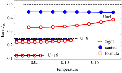
Figure 1: Bare exchange interaction as function of temperature for different values $U$, computed from the formula Eq. (4) (red open circles) and from the canted geometry Eq. (5) (blue solid discs). For large $U$ the calculations show excellent agreement with the analytical result $|J^{a}_{\mathrm{ex}}|=2t_{0}^{2}/U$ indicated with dashed lines.

Before exploring nonequilibrium, it is illustrative to evaluate the exchange interaction (4) in the familiar equilibrium case. For the Mott insulator at half-filling, the static exchange interaction at zero temperature can be obtained from a perturbation expansion in the hopping, which yields $|J_{\mathrm{ex}}^{a}|=2t_{0}^{2}/U$. In Fig. 1, we compare the analytical value $|J_{\mathrm{ex}}^{a}|$ (dashed lines) and the bare exchange interaction $|J_{\mathrm{ex}}^{0}|=|J_{\mathrm{12}}^{0}|$ computed from the collinear DMFT solution using Eq. (4) (red circles) as function of temperature for three values of $U$. In addition, we solve the DMFT equations for the antiferromagnetic Mott insulator in a weak transverse field of strength $B_{x}$ and obtain an estimate $|J_{\mathrm{ex}}^{c}|=|B_{x}/4\langle S_{x}\rangle|$ by comparing the canting $\langle S_{x}\rangle$ of spins to the prediction from a rigid macrospin model Eq. (5) in the static limit (blue solid disks). We choose $B_{x}=0.64t_{0}^{2}/U$, such that the canting angle at low temperature is about 10 degrees for all $U$. At large $U$, we find excellent agreement between $J_{\mathrm{ex}}^{a}$, $J_{\mathrm{ex}}^{0}$, and $J_{\mathrm{ex}}^{c}$, where deviations between $J_{\mathrm{ex}}^{c}$ and $J_{\mathrm{ex}}^{a}$ are on the order of $(t_{0}/U)^{2}$, which also confirms the validity of the DMFT approximation for studying exchange interactions. For smaller $U$, the deviation of $J_{\mathrm{ex}}^{0}$ from $J_{\mathrm{ex}}^{c}$ becomes more pronounced, up to 25% at $U=4$. The differences between the two Eqs. (4) and (5) may have several possible origins: (i) At small values of $U$, the rigid macrospin model is no longer valid, because retardation effects in $A(t,t^{\prime})$ become relevant, (ii) vertex corrections to Eq. (2) become important, or (iii) $J_{\mathrm{ex}}^{0}$ is a nearest-neighbor interaction while Eq. (5) also takes into account next-nearest-neighbor terms. Below we will study nonequilibrium exchange at large values of $U$. Nevertheless, for moderate $U$, where retardation effects to the exchange become important, we can still use Eq. (5) as a heuristic measure for $J_{\text{ex}}$, in the sense that it is the best estimate of an instantaneous exchange interaction which is in accordance with an observed spin dynamics.

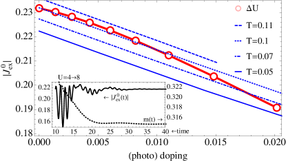
Figure 2: Comparison of the nonequilibrium exchange interaction (open circles) in the quasistationary state after an interaction quench $\Delta U$ in the Bethe lattice with the equilibrium exchange interaction of the chemically doped model (solid symbols) for $U=8$ and different temperatures. The inset shows the bare time-dependent exchange interaction (solid line) and staggered magnetization (dashed line) caused by the quench $U=4\rightarrow 8$.

Next, we investigate how fast $J_{\text{ex}}$ can be modified under electronic nonequilibrium conditions, which we generate by suddenly changing $U$. It was recently demonstrated that after such an interaction quench the order parameter $m$ quickly relaxes to a quasistationary but nonthermal value Werner et al. (2012) that is protected from further decay by the slow recombination rate of doublons and holes Eckstein and Werner (2011); Sensarma et al. (2010); Lenarčič and Prelovšek (2013); Moritz et al. (2013). This transient state resembles properties of a photodoped system in which charge carriers are created by a short laser pulse. We will refer to the induced change of the doublon and hole densities $d$ and $h$ with respect to their equilibrium values $d_{0}$ and $h_{0}$ as photodoping $\Delta n=d+h-d_{0}-h_{0}=2(d-d_{0})$. The inset of Fig. 2 shows the evolution of the time-dependent nonequilibrium exchange interaction (solid line) and order parameter (dashed line) for a quench $U=4\rightarrow 8$. [A Gaussian window $\exp(-s^{2}/w^{2})$ of length $w=10t_{0}/\pi$ was used in Eq. (3) to ensure a smooth cut off of the upper integration limit.] We find that $|J_{\mathrm{ex}}^{0}|$, like $m$, becomes stationary already on an electronic time scale, which shows the emergence of a spin Hamiltonian on the timescale of a few tens of inverse hoppings.

To study how effective $J_{\mathrm{ex}}$ is modified, we evaluate it in the quasistationary state after different excitation strengths $\Delta U=U_{\text{f}}-U_{\text{i}}=0,\ldots,4$, with final $U_{\text{f}}=8$. The result is shown by red open circles in Fig. 2 as a function of ”photo-doping” $\Delta n$, demonstrating a reduction of $J_{\mathrm{ex}}$ to a value significantly below the equilibrium difference $J_{\text{ex}}^{0}(U_{\text{i}})-J_{\text{ex}}^{0}(U_{\text{f}})$. The results are independent of a Gaussian cutoff in Eq. (3) for $w=60t_{0}/\pi$. Only for the largest $\Delta U$ do we find a slight dependence on $w$ that indicates that $J_{\mathrm{ex}}^{0}$ is not yet fully stationary. Furthermore, the blue lines in Fig. 2 show the equilibrium exchange interaction at chemical doping for different temperatures. These results confirm the conclusions obtained from analyzing the electronic spectrum Werner et al. (2012), that properties of the photodoped state with added doublons and holes resemble those of the chemically doped state with the same total number of carriers: Adding doublons and holes causes an ultrafast weakening, or “quenching” of the exchange interaction by an amount comparable to that of chemical doping. Qualitatively, the weakening of the antiferromagnetic exchange can result from a lowering of the kinetic energy of mobile carriers in a parallel spin alignment (for $U=\infty$ and small doping ferromagnetism is favored Nagaoka (1966)).

Photoexcitation.— To further demonstrate the possibility of changing $J_{\mathrm{ex}}$ in a setup that is closer to the laser excitation of condensed-matter systems, we study the Hubbard model driven by an external electric field. This is implemented for the infinite-dimensional hypercubic lattice with density of states $D(\epsilon)=\exp(-\epsilon^{2})/\sqrt{\pi}$, with the electric field pointing along the body diagonal Aoki et al. (2014); Turkowski and Freericks (2005). Photoexcited carriers are created by a single-cycle pulse $E(t)=E_{0}\sin(\omega t)\exp[-\alpha(t-t_{c})^{2}]$, $t_{c}=\pi/\omega$, $\alpha=4.6/t_{c}^{2}$ with a Gaussian envelope and a center frequency of $\omega=U$. To directly measure the transverse spin dynamics associated with $J_{\text{ex}}$, we study the system in a canted geometry induced by a homogeneous magnetic field $B_{x}$. Before laser excitation, the system is prepared in equilibrium with a canting angle determined by the balance of $B_{x}$ and $J_{\text{ex}}$. When $J_{\text{ex}}$ is changed, this balance will be broken and a spin resonance will be excited. Such spin resonances can, in principle, be detected experimentally using magneto-optical techniques Kirilyuk et al. (2010) and THz spectroscopy Nishitani et al. (2010). In our simulations, we extract the nonequilibrium exchange interaction by comparing the spin dynamics obtained within DMFT to the rigid macrospin model, cf. Eq. (5). The results of this approach are shown in Fig. 3, computed at $U=8$, $B_{x}=0.01$, and initial temperature $T=0.03$. The top panel shows that the sublattice magnetization is initially in the $x$-$z$ plane. Light to dark colors indicate excitation strengths ranging from $|E_{0}|/t_{0}=1$ to $5.5$. The bottom panel shows $\Delta J_{\mathrm{ex}}^{0}\sim\langle\dot{S}_{1y}\rangle/\langle S_{1z}\rangle$, cf. Eq. (5), where $\langle\dot{S}_{1y}\rangle$ is computed from the time trace of $\langle S_{1y}(t)\rangle$. We observe three different time scales in our simulations: (i) Fast $1/U$ oscillations on the timescale of the laser excitation, as most clearly seen in the bottom panel. This characterizes the stabilization of the local magnetic moments. (ii) Relaxation of the order parameter and the exchange interaction. (iii) The onset of rigid rotation of the spin sublattices at quasistationary values $|\langle\mathbf{S}_{1}\rangle|$ and $J^{c}_{\text{ex}}$. We estimate the time $t_{*}$ that it takes for $J^{c}_{\text{ex}}$ to become stationary from $J^{c}_{\text{ex}}(t_{*})-J^{c}_{\text{ex}}(t_{\text{max}})<\varepsilon$, where $\varepsilon$ is the numerical accuracy. The values $t_{*}$, which are indicated as dots in the bottom panel of Fig. 3, show that a quasistationary state and rigid spin dynamics emerge after a few tens of inverse hoppings, similar as for the sudden change of $U$. This relaxation time increases with the excitation density, as the critical excitation for melting the antiferromagnetic order is approached, but is much shorter than the period of spin precession in the field, which supports the interpretation that photoexcitation causes an ultrafast quenching of $J_{\mathrm{ex}}$. Furthermore, we find that direct photoexcitation has a similar effect as the interaction quench; i.e., the efficiency of the modification of $J_{\text{ex}}$ is determined by the number of photoexcited carriers. This is demonstrated in Fig. 4 by plotting the extracted exchange interaction in the quasistationary state as a function of the photodoping, together with equilibrium calculations in the canted geometry with chemical doping. In the hypercubic lattice, we observe that photoexcitation modifies $J_{\textrm{ex}}^{c}$ slightly stronger than chemical doping. In addition, there is a more pronounced temperature dependence of $J_{\textrm{ex}}^{c}$ in equilibrium. Both effects might be related to a slightly different dynamics of low-energy (photo-) doped carriers in the Bethe lattice and the hypercubic lattice, where the latter does not have a sharp band edge in the density of states.

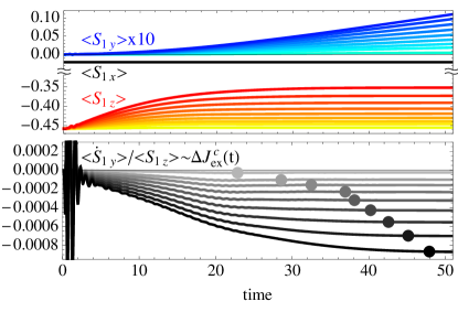
Figure 3: Induced spin dynamics (top) and modification of the exchange interaction (bottom) caused by excitation with an electric field (hypercubic lattice, $U=8$).

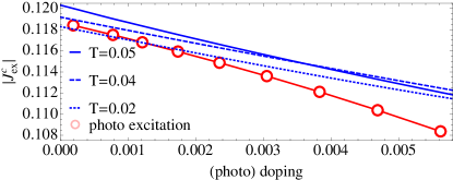
Figure 4: Comparison of the nonequilibrium exchange interaction (red open circles) computed from the induced precession (Fig. 3), with the equilibrium exchange interaction in the chemically doped system (blue lines).

In summary, we report that photoexcitation causes an ultrafast quenching of the exchange interaction in a Mott insulator. An effectively static $J_{\mathrm{ex}}$ can be defined already on the ultrafast time scale on the order of a few tens of inverse hopping times, which is similar to the relaxation time of the order parameter. The reduction of $J_{\mathrm{ex}}$ is comparable to that of a chemically doped state when measured in terms of the total number of excited carriers. These results demonstrate intriguing possibilities to control magnetic order without magnetic fields. Similar, or even more efficient ways to control $J_{\text{ex}}$ under nonequilibrium conditions might be found by extending our work to more complex multi-band systems such as the prototype Mott-insulator V₂O₃ Liu et al. (2011) and to materials with different exchange mechanisms.

Supplementary material

Appendix A Implementation of nonequilibrium DMFT with a transverse magnetic field

In the supplementary material we describe in detail how we implement the nonequilibrium DMFT for the antiferromagnetic phase of the Hubbard model in a transverse magnetic field,

$$H= -\sum_{\langle ij\rangle\sigma}t_{ij}\,c_{i\sigma}^{\dagger}c_{j\sigma}+U\sum_{j}n_{j\uparrow}n_{j\downarrow}+B_{x}\sum_{j}S_{jx}-\mu\sum_{j\sigma}n_{j\sigma}.$$ (6)

Apart from the incorporation of spin-flip terms in the DMFT impurity action and the self-consistency relations, the resulting equations are a straightforward extension of the equations for the paramagnetic phase and the collinear antiferromagnet, which have been described previously Aoki et al. (2014); Eckstein and Werner (2010).

A.1 The impurity model

To describe a magnetically ordered system, we introduce Keldysh Green’s functions which are $2\times 2$ matrices in spin-space,

$$\hat{G}_{jj^{\prime}}(t,t^{\prime})=-i\langle\,\mathcal{T}_{\mathcal{C}}\hat{\psi}_{j}(t)\hat{\psi}_{j^{\prime}}^{\dagger}(t)\,\rangle_{\mathcal{S}}$$ (7)

$$=\begin{pmatrix}-i\langle\mathcal{T}_{\mathcal{C}}\,c_{j\uparrow}(t)\,c_{j^{\prime}\uparrow}^{\dagger}(t)\,\rangle_{\mathcal{S}}&-i\langle\mathcal{T}_{\mathcal{C}}\,c_{j\uparrow}(t)\,c_{j^{\prime}\downarrow}^{\dagger}(t)\,\rangle_{\mathcal{S}}\\ -i\langle\mathcal{T}_{\mathcal{C}}\,c_{j\downarrow}(t)\,c_{j^{\prime}\uparrow}^{\dagger}(t)\,\rangle_{\mathcal{S}}&-i\langle\mathcal{T}_{\mathcal{C}}\,c_{j\downarrow}(t)\,c_{j^{\prime}\downarrow}^{\dagger}(t)\,\rangle_{\mathcal{S}}\end{pmatrix}.$$ (8)

Here $\hat{\psi}_{j}$ is the spinor

$$\hat{\psi}_{j}=\begin{pmatrix}c_{j\uparrow}\\ c_{j\downarrow}\end{pmatrix},$$ (9)

$\mathcal{C}$ is the $L$-shaped Keldysh contour that extends from $0$ to some maximum time $t_{\text{max}}$ along the real axis, back to $0$, and to $-i\beta$ along the imaginary time axis, and

$$\langle\mathcal{T}_{\mathcal{C}}\cdots\rangle_{\mathcal{S}}\equiv\text{tr}\big{[}\mathcal{T}_{\mathcal{C}}e^{\mathcal{S}}\,\cdots\big{]}\,/\,\text{tr}\big{[}\mathcal{T}_{\mathcal{C}}e^{\mathcal{S}}\,\big{]}$$ (10)

denotes the contour-ordered expectation value for an action $\mathcal{S}$; the action for the lattice model (6) is given by $\hat{\mathcal{S}}=-i\int_{\mathcal{C}}d\bar{t}\,\hat{H}(\bar{t})$. We follow Ref. Aoki et al. (2014) for the notation for Keldysh Green’s and their convolution and time-derivatives along $\mathcal{C}$.

The antiferromagnetic DMFT solution is obtained on a bipartite lattice at and close to half-filling. The local Green’s function $\hat{G}_{\alpha}$ for a site on sub-lattice $\alpha=A,B$ of the bipartite lattice is obtained from an impurity model with action

$$\hat{\mathcal{S}}_{\alpha}=-i\int_{\mathcal{C}}dt\,H_{\text{loc},\alpha}(t)-i\int_{\mathcal{C}}\!dtdt^{\prime}\,\hat{\psi}^{\dagger}(t)\hat{\Delta}_{\alpha}(t,t^{\prime})\hat{\psi}(t^{\prime}),$$ (11)

where $H_{\text{loc},\alpha}(t)$ is the local part of Hamiltonian (6), and $\hat{\Delta}_{\alpha}(t,t^{\prime})$ is the hybridization matrix, which is later determined self-consistently.

In order to compute compute the impurity Green’s function

$$\hat{G}_{\alpha}(t,t^{\prime})=-i\langle\,\mathcal{T}_{\mathcal{C}}\hat{\psi}(t)\hat{\psi}^{\dagger}(t)\,\rangle_{\hat{\mathcal{S}}_{\alpha}},$$ (12)

we use the lowest strong-coupling impurity solver Eckstein and Werner (2010) (non-crossing approximation, NCA), which is a self-consistent expansion in the hybridization function $\hat{\Delta}_{\alpha}(t,t^{\prime})$. The hybridization expansion can be formulated in terms of pseudo-particle propagators ${\mathcal{G}}_{nm}$, whose flavor indices $n$, $m$ correspond to the many-body states of the impurity. These propagators satisfy a Dyson equation, with a self-energy ${\mathfrak{S}}$ that is given by a diagrammatic expansion in the hybridization function. In the present case, a basis of the local Hilbert space at the impurity model is given by the four states $|0\rangle$, $|\sigma\rangle\equiv c_{\sigma}^{\dagger}|0\rangle$ (for $\sigma=\pm$), and $|2\rangle\equiv c_{\uparrow}^{\dagger}c_{\downarrow}^{\dagger}|0\rangle$. Because the $H_{\text{loc}}$ and $\hat{\Delta}_{\alpha}(t,t^{\prime})$ allow spin-flip terms, pseudo-particle propagators ${\mathcal{G}}_{nm}$ are only diagonal in particle number of $|n\rangle$ and $|m\rangle$, but not in spin. Hence, we introduce three propagators, ${\mathcal{G}}^{(0)}\equiv{\mathcal{G}}_{|0\rangle,|0\rangle}$, ${\mathcal{G}}^{(2)}\equiv{\mathcal{G}}_{|2\rangle,|2\rangle}$, and ${\mathcal{G}}^{(1)}_{\sigma\sigma^{\prime}}\equiv{\mathcal{G}}_{|\sigma\rangle,|\sigma^{\prime}\rangle}$, and corresponding self-energies ${\mathfrak{S}}^{(n)}(t,t^{\prime})$, $n=0,1,2$. From the the diagrammatic rules for a general multi-orbital case as stated in Ref. Eckstein and Werner (2010), we obtain

$${\mathfrak{S}}^{(0)}(t,t^{\prime}) =-i\sum_{\sigma,\sigma^{\prime}}{\mathcal{G}}^{(1)}_{\sigma\sigma^{\prime}}(t,t^{\prime})\Delta_{\sigma^{\prime}\sigma}(t^{\prime},t)$$ (13)

$${\mathfrak{S}}^{(1)}_{\sigma\sigma^{\prime}}(t,t^{\prime}) =i{\mathcal{G}}^{(0)}(t,t^{\prime})\Delta_{\sigma\sigma^{\prime}}(t,t^{\prime})-i\bar{\sigma}\bar{\sigma}^{\prime}{\mathcal{G}}^{(2)}(t,t^{\prime})\Delta_{\bar{\sigma}^{\prime}\bar{\sigma}}(t^{\prime},t)$$ (14)

$${\mathfrak{S}}^{(2)}(t,t^{\prime}) =i\sum_{\sigma\sigma^{\prime}}\bar{\sigma}\bar{\sigma}^{\prime}{\mathcal{G}}^{(1)}_{\sigma\sigma^{\prime}}(t,t^{\prime})\Delta_{\bar{\sigma}\bar{\sigma}^{\prime}}(t,t^{\prime}).$$ (15)

Finally, the local Green’s function is given by evaluation of the “bubble diagram” Eckstein and Werner (2010)

$$G_{\sigma\sigma^{\prime}}(t,t^{\prime}) =i{\mathcal{G}}^{(0)}(t^{\prime},t){\mathcal{G}}^{(1)}_{\sigma\sigma^{\prime}}(t,t^{\prime})-i\sigma\sigma^{\prime}{\mathcal{G}}^{(1)}_{\bar{\sigma}^{\prime}\bar{\sigma}}(t^{\prime},t){\mathcal{G}}^{(2)}(t,t^{\prime}).$$ (16)

A.2 DMFT self-consistency for the Bethe lattice

For a Bethe lattice with nearest neighbor hopping $t_{ij}\equiv t_{0}/\sqrt{Z}$ in the limit $Z\to\infty$, which has a semi-elliptic density of states $D(\epsilon)=\sqrt{4-\epsilon^{2}}/2\pi$ for $t_{0}=1$, the hybridization function is determined by the closed form self-consistency equation Georges et al. (1996)

$$\hat{\Delta}_{\alpha}(t,t^{\prime})=t_{0}^{2}\hat{G}_{\bar{\alpha}}(t,t^{\prime}),$$ (17)

where $\bar{\alpha}=B$($A$) for $\alpha=A$($B$). The NCA equations together with Eq. (17) provide a closed set of equations that is numerically propagated in time as described in Ref. Aoki et al. (2014).

A.3 DMFT self-consistency for the hypercubic lattice

To solve the DMFT equation on a cubic lattice with $A/B$ sub-lattice symmetry breaking, we let ${\mathcal{L}^{\prime}}$ denote the magnetic superlattice of points $\bm{R}_{j}$, and $\mathcal{L}$ is the full lattice with atoms at coordinates $\bm{r}_{j\alpha}=\bm{R}_{j}+\bm{\delta}_{\alpha}$, $\alpha=A,B$. For example, we can choose ${\mathcal{L}^{\prime}}$ as the $A$-sublattice of the bipartite cubic lattice, such that $\bm{\delta}_{A}=0$, $\bm{\delta}_{B}=(1,0,...)$. We then introduce the Fourier transform with respect to the coordinate $\bm{R}_{j}$,

$$c_{{\bm{K}}\alpha\sigma} =\frac{1}{\sqrt{L^{\prime}}}\sum_{j\in{\mathcal{L}^{\prime}}}e^{-i{\bm{K}}({\bm{R}}_{j}+\bm{\delta}_{\alpha})}c_{j\alpha\sigma},$$ (18)

$$c_{j\alpha\sigma} =\frac{1}{\sqrt{L^{\prime}}}\sum_{{\bm{K}}\in{\mathcal{B}^{\prime}}}e^{i{\bm{K}}({\bm{R}}_{j}+\bm{\delta}_{\alpha})}c_{{\bm{K}}\alpha\sigma},$$ (19)

where $L^{\prime}$ is the number points in ${\mathcal{L}^{\prime}}$, and ${\mathcal{B}^{\prime}}$ is the first Brillouin zone of the magnetic superlattice. To describe the broken symmetry phase, we introduce super-spinors

$$\hat{\Psi}_{{\bm{K}}}=\begin{pmatrix}c_{{\bm{K}},A,\uparrow}\\ c_{{\bm{K}},A,\downarrow}\\ c_{{\bm{K}},B,\uparrow}\\ c_{{\bm{K}},B,\downarrow}\end{pmatrix}\equiv\begin{pmatrix}\hat{\psi}_{{\bm{K}},A}\\ \hat{\psi}_{{\bm{K}},B}\end{pmatrix},$$ (20)

and corresponding Green’s functions

$$\hat{G}_{\bm{K}}(t) =-i\langle\mathcal{T}_{\mathcal{C}}\hat{\Psi}_{\bm{K}}(t)\hat{\Psi}_{\bm{K}}^{\dagger}(t^{\prime})\rangle$$ (21)

$$\equiv\begin{pmatrix}\hat{G}_{{\bm{K}},AA}(t,t^{\prime})&\hat{G}_{{\bm{K}},AB}(t,t^{\prime})\\ \hat{G}_{{\bm{K}},BA}(t,t^{\prime})&\hat{G}_{{\bm{K}},BB}(t,t^{\prime})\end{pmatrix},$$ (22)

where the second expression is a block-matrix with entries $\hat{G}_{{\bm{K}},\alpha\alpha^{\prime}}(t,t^{\prime})=-i\langle\mathcal{T}_{\mathcal{C}}\hat{\psi}_{{\bm{K}},\alpha}(t)\hat{\psi}_{{\bm{K}},\alpha^{\prime}}^{\dagger}(t^{\prime})\rangle$. With this, the quadratic part of the Hamiltonian (6) can be rewritten as $\sum_{{\bm{K}}\in{\mathcal{B}^{\prime}}}\hat{\Psi}_{{\bm{K}}}^{\dagger}\hat{H}_{\bm{K}}\hat{\Psi}_{{\bm{K}}}$, with

$$\hat{H}_{{\bm{K}}}=\begin{pmatrix}\hat{H}_{loc,A}&\hat{\epsilon}_{\bm{K}}\\ \hat{\epsilon}_{\bm{K}}&\hat{H}_{loc,B}\end{pmatrix},$$ (23)

where $\hat{H}_{loc,A}=\hat{H}_{loc,B}=\hat{\sigma}_{x}B_{x}$ and $\hat{\epsilon}_{\bm{K}}=\epsilon_{\bm{K}}\hat{1}$, with the $2\times 2$ unit matrix $\hat{1}$. The electronic dispersion $\epsilon_{\bm{K}}$ may be time-dependent due to inclusion of a external electric field via the Peierls substitution (see below). The Dyson equation has a $4\!\times\!4$-structure,

$$\hat{G}_{\bm{K}}^{-1}(t,t^{\prime})=\delta_{\mathcal{C}}(t,t^{\prime})[(i\partial_{t}+\mu)\hat{1}-\hat{H}_{\bm{K}}]-\hat{\Sigma}(t,t^{\prime}),$$ (24)

with the spatially local self energy

$$\hat{\Sigma}(t,t^{\prime}) =\begin{pmatrix}\hat{\Sigma}_{A}(t,t^{\prime})&0\\ 0&\hat{\Sigma}_{B}(t,t^{\prime})\end{pmatrix},$$ (25)

$$\hat{\Sigma}_{\alpha}(t,t^{\prime}) =\begin{pmatrix}\Sigma_{\alpha,\uparrow\uparrow}(t,t^{\prime})&\Sigma_{\alpha,\uparrow\downarrow}(t,t^{\prime})\\ \Sigma_{\alpha,\downarrow\uparrow}(t,t^{\prime})&\Sigma_{\alpha,\downarrow\downarrow}(t,t^{\prime})\end{pmatrix}.$$ (26)

Numerically, it is convenient to solve the DMFT equations without explicitly solving for the self energy. By introducing $\hat{Z}_{\alpha}=[i\partial_{t}+\mu-\hat{H}_{loc,\alpha}-\hat{\Sigma}_{\alpha}]^{-1}$, the impurity Dyson equation reads

$$\hat{G}_{\alpha}=\hat{Z}_{\alpha}+\hat{Z}_{\alpha}\ast\hat{\Delta}_{\alpha}\ast\hat{G}_{\alpha},$$ (27)

and the lattice Dyson equation is given by

$$\hat{G}_{\bm{K}}=\begin{pmatrix}\hat{Z}_{A}&0\\ 0&\hat{Z}_{B}\end{pmatrix}+\begin{pmatrix}\hat{Z}_{A}&0\\ 0&\hat{Z}_{B}\end{pmatrix}\ast\begin{pmatrix}0&\hat{\epsilon}_{\bm{K}}\\ \hat{\epsilon}_{\bm{K}}&0\end{pmatrix}\ast\hat{G}_{\bm{K}}.$$ (28)

The lattice Dyson equation can be written explicitly for its four $2\times 2$ components,

$$\hat{G}_{{\bm{K}},AA} =\hat{Z}_{A}+\hat{Z}_{A}\ast\hat{\epsilon}_{\bm{K}}\ast\hat{Z}_{B}\ast\hat{\epsilon}_{\bm{K}}\ast\hat{G}_{{\bm{K}},AA},$$ (29)

$$\hat{G}_{{\bm{K}},BB} =\hat{Z}_{B}+\hat{Z}_{B}\ast\hat{\epsilon}_{\bm{K}}\ast\hat{Z}_{A}\ast\hat{\epsilon}_{\bm{K}}\ast\hat{G}_{{\bm{K}},BB},$$ (30)

$$\hat{G}_{{\bm{K}},AB} =\hat{Z}_{A}\ast\hat{\epsilon}_{\bm{K}}\ast\hat{G}_{{\bm{K}},BB},$$ (31)

$$\hat{G}_{{\bm{K}},BA} =\hat{Z}_{B}\ast\hat{\epsilon}_{\bm{K}}\ast\hat{G}_{{\bm{K}},AA},$$ (32)

(where we have reinserted the expressions for $\hat{G}_{{\bm{K}},AB}$ and $\hat{G}_{{\bm{K}},BA}$ into the equations for $\hat{G}_{{\bm{K}},AA}$ and $\hat{G}_{{\bm{K}},BB}$.) By summing these equations over ${\bm{K}}$ and comparing with the impurity Dyson equation, we then obtain an explicit equation for the hybridization function (for $\alpha=A,B$). For this it is convenient to introduce the moments

$$\hat{G}_{\alpha} =\frac{1}{L^{\prime}}\sum_{{\bm{K}}\in{\mathcal{B}^{\prime}}}\hat{G}_{{\bm{K}},\alpha\alpha}$$ (33)

$$\hat{G}_{\alpha}^{(1)} \equiv\frac{1}{L^{\prime}}\sum_{{\bm{K}}\in{\mathcal{B}^{\prime}}}\hat{\epsilon}_{\bm{K}}\ast\hat{Z}_{\bar{\alpha}}\ast\hat{\epsilon}_{\bm{K}}\ast\hat{G}_{{\bm{K}},\alpha\alpha}$$ (34)

$$=\hat{\Delta}_{\alpha}\ast G_{\alpha},$$ (35)

$$\hat{G}_{\alpha}^{(2)} \equiv\frac{1}{L^{\prime}}\sum_{{\bm{K}}\in{\mathcal{B}^{\prime}}}\hat{\epsilon}_{\bm{K}}\ast\hat{Z}_{\bar{\alpha}}\ast\hat{\epsilon}_{\bm{K}}\ast\hat{G}_{{\bm{K}},\alpha\alpha}\ast\hat{\epsilon}_{\bm{K}}\ast\hat{Z}_{\bar{\alpha}}\ast\hat{\epsilon}_{\bm{K}}$$

$$+\frac{1}{L^{\prime}}\sum_{{\bm{K}}\in{\mathcal{B}^{\prime}}}\hat{\epsilon}_{\bm{K}}\ast\hat{Z}_{\bar{\alpha}}\ast\hat{\epsilon}_{\bm{K}}$$ (36)

$$=\hat{\Delta}_{\alpha}+\hat{\Delta}_{\alpha}\ast G_{\alpha}\ast\hat{\Delta}_{\alpha}.$$ (37)

Here Eqs. (35) and (37) follow from comparison with the impurity Dyson equation (27). Combining the two equations, we obtain

$$(\hat{1}+\hat{G}_{\alpha}^{(1)})\ast\hat{\Delta}_{\alpha}=\hat{G}^{(2)}_{\alpha},$$ (38)

from which the hybridization can be determined, thus closing the DMFT self-consistency.

Throughout this work we consider magnetic fields along $x$, perpendicular to the antiferromagnetic order parameter. In this case, the system is invariant under a translation by one lattice constant and spin rotation by $\pi$ around the axis of the $B$-field. This symmetry can be used to relate local quantities at the $A$ and $B$ sites, i.e.,

$$\hat{\Sigma}_{B} =\hat{\sigma}_{x}\hat{\Sigma}_{A}\hat{\sigma}_{x},$$ (39)

and analogous for the functions $\hat{Z}_{\alpha}$, $\hat{G}_{\alpha}$, and $\hat{\Delta}_{\alpha}$. Explicitly,

$$\begin{pmatrix}\Sigma_{B,\uparrow\uparrow}(t,t^{\prime})&\Sigma_{B,\uparrow\downarrow}(t,t^{\prime})\\ \Sigma_{B,\downarrow\uparrow}(t,t^{\prime})&\Sigma_{B,\downarrow\downarrow}(t,t^{\prime})\end{pmatrix} =\begin{pmatrix}\Sigma_{A,\downarrow\downarrow}(t,t^{\prime})&\Sigma_{A,\downarrow\uparrow}(t,t^{\prime})\\ \Sigma_{A,\uparrow\downarrow}(t,t^{\prime})&\Sigma_{A,\uparrow\uparrow}(t,t^{\prime})\end{pmatrix}.$$ (40)

This symmetry leads to a considerable reduction of the numerical complexity, because one can make the $4\times 4$ Dyson equation (28) $2\times 2$ block-diagonal with the basis change

$$\hat{V}=\frac{1}{\sqrt{2}}\begin{pmatrix}\hat{1}&\hat{\sigma}_{x}\\ \hat{\sigma}_{x}&-\hat{1}\end{pmatrix}.$$ (41)

The symmetry (39) implies

$$\hat{V}\begin{pmatrix}\hat{Z}_{A}&0\\ 0&\hat{Z}_{B}\end{pmatrix}\hat{V}^{\dagger}=\begin{pmatrix}\hat{Z}_{A}&0\\ 0&\hat{Z}_{B}\end{pmatrix},$$ (42)

and we have

$$\hat{V}\begin{pmatrix}0&\hat{\epsilon}_{\bm{K}}\\ \hat{\epsilon}_{\bm{K}}&0\end{pmatrix}\hat{V}^{\dagger}=\begin{pmatrix}\epsilon_{\bm{K}}\hat{\sigma}_{x}&0\\ 0&-\epsilon_{\bm{K}}\hat{\sigma}_{x}\end{pmatrix}.$$ (43)

Thus the Dyson equation for the transformed $4\times 4$ Green’s functions

$$\tilde{G}_{\bm{K}}(t,t^{\prime})=\hat{V}\hat{G}_{\bm{K}}(t,t^{\prime})\hat{V}^{\dagger}.$$ (44)

is block-diagonal: When we introduce the notation

$$\tilde{G}_{\bm{K}}\equiv\begin{pmatrix}\hat{G}_{\bm{K}}^{+}&0\\ 0&\hat{\sigma}_{x}\hat{G}_{\bm{K}}^{-}\hat{\sigma}_{x}\end{pmatrix},$$ (45)

(the $\hat{\sigma}_{x}$ in the second coefficients are introduced for convenience), the two blocks are obtained by solving two Dyson equations,

$$\hat{Z}_{A}+\hat{Z}_{A}\ast\epsilon_{\bm{K}}\hat{\sigma}_{x}\ast\hat{G}_{\bm{K}}^{+}=\hat{G}_{\bm{K}}^{+}$$ (46)

$$\hat{Z}_{A}-\hat{Z}_{A}\ast\epsilon_{\bm{K}}\hat{\sigma}_{x}\ast\hat{G}_{\bm{K}}^{-}=\hat{G}_{\bm{K}}^{-},$$ (47)

where we have again used the symmetry $\hat{Z}_{B}=\hat{\sigma}_{x}\hat{Z}_{A}\hat{\sigma}_{x}$ in the second equation. The back-transformation to the original basis, $\hat{G}_{\bm{K}}=\hat{V}^{\dagger}\hat{G}_{\bm{K}}\hat{V}$, gives

$$\hat{G}_{\bm{K}}=\frac{1}{2}\begin{pmatrix}\hat{G}_{\bm{K}}^{+}+\hat{G}_{\bm{K}}^{-}&(\hat{G}_{\bm{K}}^{+}-\hat{G}_{\bm{K}}^{-})\hat{\sigma}_{x}\\ \hat{\sigma}_{x}(\hat{G}_{\bm{K}}^{+}-\hat{G}_{\bm{K}}^{-})&\hat{\sigma}_{x}(\hat{G}_{\bm{K}}^{+}+\hat{G}_{\bm{K}}^{-})\hat{\sigma}_{x}\end{pmatrix}.$$ (48)

The ${\bm{K}}$-summed quantities (33), (34), and (36) are thus obtained as

$$\hat{G}_{A} =\frac{1}{2L^{\prime}}\sum_{{\bm{K}}\in{\mathcal{B}^{\prime}}}\hat{G}_{\bm{K}}^{+}+\hat{G}_{\bm{K}}^{-}$$ (49)

$$\hat{G}_{A}^{(1)} =\frac{1}{2L^{\prime}}\sum_{{\bm{K}}\in{\mathcal{B}^{\prime}}}\epsilon_{\bm{K}}\hat{\sigma}_{x}\ast(\hat{G}_{\bm{K}}^{+}-\hat{G}_{\bm{K}}^{-})$$ (50)

$$\hat{G}_{A}^{(2)} =\frac{1}{2L^{\prime}}\sum_{{\bm{K}}\in{\mathcal{B}^{\prime}}}\epsilon_{\bm{K}}\hat{\sigma}_{x}\ast(\hat{G}_{\bm{K}}^{+}+\hat{G}_{\bm{K}}^{-})\ast\hat{\sigma}_{x}\epsilon_{\bm{K}}.$$ (51)

Here we have used Eqs. (31) and (32) in Eqs. (34), and (36), and then replaced $\hat{G}_{{\bm{K}}\alpha,\alpha^{\prime}}$ by the explicit expressions obtained from Eq. (48). Because all convolutions involve the time-local functions $\epsilon_{\bm{K}}$, they are evaluated without numerical cost.

The final set of DMFT equations, to be solved successively timestep after timestep, is thus given by: (i) Solve one impurity model (the one on the $A$-lattice), i.e, compute $\hat{G}_{A}$ [Eq. (12)] from the action (11) with hybridization $\hat{\Delta}_{A}$. (ii) Solve Eq. (27) for $\hat{Z}_{A}$. (iii) Solve two equations (46) and (47) for $\hat{G}_{\bm{K}}^{+}$ and $\hat{G}_{\bm{K}}^{-}$. (iv) Evaluate the sums Eq. (49) to (51). (v) Compute the new hybridization function $\hat{\Delta}_{A}$ from Eq. (38).

Finally, the summation over ${\bm{K}}$ is reduced to an integral over the density of states, as described in Ref. Turkowski and Freericks (2005). We consider a cubic lattice with pure nearest neighbor hopping, and an electric field $\bm{E}(t)=E(t)(1,1,1,...)$ which is pointing along the body-diagonal of the unit cell. Then

$$\epsilon_{\bm{K}} =\frac{-2t^{*}}{\sqrt{2d}}\sum_{\alpha=1}^{d}\cos(k_{\alpha}-A(t))$$

$$=\cos(A(t))\epsilon^{0}_{\bm{K}}+\sin(A(t))\bar{\epsilon}^{0}_{\bm{K}},$$ (52)

where $\epsilon^{0}_{\bm{K}}$ and $\bar{\epsilon}^{0}_{\bm{K}}$ are band energies in the zero-field case, and $A(t)$ is the vector potential. The equations use a gauge with zero scalar potential, i.e., $E(t)=-\partial_{t}A(t)$, and the unit of the field is $\text{hopping}/(e\times\text{lattice constant})$. Since all functions depend on ${\bm{K}}$ only via $\epsilon^{0}_{\bm{K}}$ and $\bar{\epsilon}^{0}_{\bm{K}}$, we can reduce the ${\bm{K}}$ sum as

$$\frac{1}{L^{\prime}}\sum_{{\bm{K}}\in{\mathcal{B}^{\prime}}}f(\epsilon^{0}_{\bm{K}},\bar{\epsilon}^{0}_{\bm{K}})=\int\!d\epsilon\,d\bar{\epsilon}\,f(\epsilon,\bar{\epsilon})D^{\prime}(\epsilon,\bar{\epsilon}),$$ (53)

with the density of states for the reduced zone

$$D^{\prime}(\epsilon,\bar{\epsilon})=\frac{1}{L^{\prime}}\sum_{{\bm{K}}\in{\mathcal{B}^{\prime}}}\delta(\epsilon-\epsilon^{0}_{\bm{K}})\delta(\bar{\epsilon}-\bar{\epsilon}^{0}_{\bm{K}}).$$ (54)

Because all points in the full BZ ${\mathcal{B}}$ can be obtained by $\{{\bm{K}},{\bm{K}}+{\bm{Q}}\}$ with ${\bm{K}}\in{\mathcal{B}^{\prime}}$ and ${\bm{Q}}=(\pi,\pi,...)$, and because $\epsilon^{0}_{{\bm{K}}+{\bm{Q}}}=-\epsilon^{0}_{{\bm{K}}}$, we can choose the reduced BZ ${\mathcal{B}^{\prime}}$ as all ${\bm{K}}$ with $\epsilon^{0}_{{\bm{K}}}<0$. Hence we have

$$D^{\prime}(\epsilon,\bar{\epsilon})=2\Theta(-\epsilon)D(\epsilon,\bar{\epsilon}),$$ (55)

where $D(\epsilon,\bar{\epsilon})$ is the density of states for the full BZ. We will work in the limit of infinite dimensions, with $D(\epsilon,\bar{\epsilon})=e^{-\epsilon^{2}}e^{-\bar{\epsilon}^{2}}$ Turkowski and Freericks (2005).

We close with the remark that the DMFT equations conserve the total spin along the direction of $\bm{B}$. The magnetic field $B_{x}$ thus determines only the time-independent expectation value of the initial field, while any time-dependence of a homogeneous magnetic field implies a trivial time-dependent rotation of the Green’s functions in spin space.

Appendix B Evaluation the exchange formulas

In this section we describe how we evaluate numerically the exchange interactions [Eq. (2) of the main text] within DMFT. In contrast to the evaluation of the DMFT self-consistency described above, this requires an explicit knowledge of the self energy. Below we discuss how the self energy $\mathit{\Sigma}_{i}(t,t^{\prime})$ is evaluated using numerical derivatives. Once $\mathit{\Sigma}_{i}(t,t^{\prime})$ is computed, the exchange interactions are evaluated by making the appropriate products and convolutions.

Within NCA, the self-consistent solution of the impurity model gives us direct access to the local Green function $G_{i}(t,t^{\prime})$ and the hybridization function $\Delta_{i}(t,t^{\prime})$ (where possible we omit the spin index $\sigma$). $\mathit{\Sigma}_{i}(t,t^{\prime})$ is related to $G_{i}(t,t^{\prime})$ and $\Delta_{i}(t,t^{\prime})$ by the impurity Dyson equation:

$$\text{i}\partial_{t}G_{i}-\left[\Delta_{i}*G_{i}\right] = 1+\left[\mathit{\Sigma}_{i}*G_{i}\right],$$ (56)

where $1$ indicates the delta function $\delta_{\mathcal{C}}(t,{t^{\prime}})$ on the Keldysh contour. To be able to handle the equal-time discontinuities of the Green’s functions and self energies analytically, we write the self-energy as $\mathit{\Sigma}_{i}=\bar{\mathit{\Sigma}_{i}}+\mathit{\Sigma}_{i}^{\prime}$. Here $\bar{\mathit{\Sigma_{i}}}(t,t^{\prime})=\delta_{\mathcal{C}}(t,{t^{\prime}})\mathit{\Sigma}^{H}_{i}(t)$ is the Hartree component of the self-energy and $\mathit{\Sigma}_{i}^{\prime}(t,{t^{\prime}})$ is the part of the self-energy which is finite at $t=t^{\prime}$.

The Hartree component is computed by invoking a first numerical derivative, indicated as $\partial_{\mathrm{N}t}$, which is evaluated only for $t={t^{\prime}}\pm\varepsilon$. Denoting $F_{i}=\mathit{\Sigma}_{i}*G_{i}$ we write the Dyson equation as:

$$F_{i} = \text{i}\partial_{t}G_{i}-1-\Delta_{i}*G_{i}$$

$$= (\text{i}\partial_{\mathrm{N}t}G_{i}+1)-1-\Delta_{i}*G_{i}=\text{i}\partial_{\mathrm{N}t}G_{i}-\Delta_{i}*G_{i}.$$

$\mathit{\Sigma}_{i}^{H\bar{\sigma}}(t)$ now follows directly from the equal time contribution $F_{i}(t,t)$. On the real-time axis we have

$$F^{>\sigma}_{i}(t,t)-F^{<\sigma}_{i}(t,t)=-\text{i}\,\mathit{\Sigma}_{i}^{H\bar{\sigma}}(t),$$ (58)

where we used that $G^{>}(t,t)-G^{<}(t,t)=-\text{i}$. On the Matsubara axis we have equivalently $F^{\sigma}_{i}(0)+F^{\sigma}_{i}(\beta)=-\mathit{\Sigma}_{i}^{H\sigma}(0)$.

To compute the component $\mathit{\Sigma}_{i}^{\prime}(t,{t^{\prime}})$ we invoke a second derivative and write the local $T$ matrix as:

$$T_{i} = \text{i}\partial_{t}F^{\dagger}_{i}-\Delta_{i}*F^{\dagger}_{i}=\left[\text{i}\partial_{t}G_{i}-\Delta_{i}*G_{i}\right]*\mathit{\Sigma}_{i}$$

$$= \left[\text{i}\partial_{\text{N}t}G_{i}+1-\Delta_{i}*G_{i}\right]*\mathit{\Sigma}_{i}$$

$$= \text{i}\partial_{\text{N}t}F^{\dagger}_{i}-\Delta_{i}*F^{\dagger}_{i}+\mathit{\Sigma}_{i}.$$

In addition, we have

$$T_{i} = \left[\text{i}\partial_{t}G_{i}-\Delta_{i}*G_{i}\right]*\mathit{\Sigma}_{i}=\mathit{\Sigma}_{i}+\mathit{\Sigma}_{i}*G_{i}*\mathit{\Sigma}_{i}$$

$$= \bar{\mathit{\Sigma}}_{i}+\mathit{\Sigma}_{i}^{\prime}+F_{i}*(\bar{\mathit{\Sigma}}_{i}+\mathit{\Sigma}_{i}^{\prime})$$

$$= \bar{\mathit{\Sigma}}_{i}+F_{i}\,\mathit{\Sigma}^{H}_{i}+(1+F_{i})*\mathit{\Sigma}_{i}^{\prime}.$$

By subtracting Eq. (B) and Eq. (B) we obtain:

$$(1+F_{i})*\mathit{\Sigma}_{i}^{\prime}=\text{i}\partial_{\text{N}t}F^{\dagger}_{i}-\Delta_{i}*F^{\dagger}_{i}-F_{i}\,\mathit{\Sigma}^{H}_{i}.$$ (61)

Finally, the self-energy $\mathit{\Sigma}_{i}^{\prime}$ is evaluated by inverting Eq. (61). This integral equation corresponds to a Volterra equation of the second kind, which is numerically well conditioned.

References

• Kirilyuk et al. (2010) A. Kirilyuk, A. V. Kimel, and T. Rasing, Rev. Mod. Phys. 82, 2731 (2010).
• Wall et al. (2009) S. Wall, D. Prabhakaran, A. T. Boothroyd, and A. Cavalleri, Phys. Rev. Lett. 103, 097402 (2009).
• Först et al. (2011) M. Först, R. I. Tobey, S. Wall, H. Bromberger, V. Khanna, A. L. Cavalieri, Y.-D. Chuang, W. S. Lee, R. Moore, W. F. Schlotter, et al., Phys. Rev. B 84, 241104 (2011).
• Li et al. (2013) T. Li, A. Patz, L. Mouchliadis, J. Yan, T. A. Lograsso, I. Perakis, and J. Wang, Nature (London) 496, 69 (2013).
• (5) M. Matsubara, A. Schroer, A. Schmehl, A. Melville, C. Becher, M. Martinez, D. Schlom, J. Mannhart, J. Kroha, and M. Fiebig, eprint arXiv:1304.2509.
• Duan et al. (2003) L.-M. Duan, E. Demler, and M. D. Lukin, Phys. Rev. Lett. 91, 090402 (2003).
• Trotzky et al. (2008) S. Trotzky, P. Cheinet, S. F lling, M. Feld, U. Schnorrberger, A. M. Rey, A. Polkovnikov, E. A. Demler, M. D. Lukin, and I. Bloch, Science 319, 295 (2008).
• Ju et al. (2004) G. Ju, J. Hohlfeld, B. Bergman, R. J. M. van de Veerdonk, O. N. Mryasov, J.-Y. Kim, X. Wu, D. Weller, and B. Koopmans, Phys. Rev. Lett. 93, 197403 (2004).
• Thiele et al. (2004) J. Thiele, M. Buess, and C. H. Back, Appl. Phys. Lett. 85, 2857 (2004).
• Rhie et al. (2003) H.-S. Rhie, H. Dürr, and W. Eberhardt, Phys. Rev. Lett. 90, 247201 (2003).
• Carley et al. (2012) R. Carley, K. Döbrich, B. Frietsch, C. Gahl, M. Teichmann, O. Schwarzkopf, P. Wernet, and M. Weinelt, Phys. Rev. Lett. 109, 057401 (2012).
• Beaurepaire et al. (1996) E. Beaurepaire, J.-C. Merle, A. Daunois, and J.-Y. Bigot, Phys. Rev. Lett. 76, 4250 (1996).
• Stanciu et al. (2007) C. D. Stanciu, F. Hansteen, A. V. Kimel, A. Kirilyuk, A. Tsukamoto, A. Itoh, and T. Rasing, Phys. Rev. Lett. 99, 047601 (2007).
• Radu et al. (2011) I. Radu, K. Vahaplar, C. Stamm, T. Kachel, N. Pontius, H. A. Dürr, T. A. Ostler, J. Barker, R. F. L. Evans, R. W. Chantrell, et al., Nature (London) 472, 205 (2011).
• Ostler et al. (2012) T. Ostler, J. Barker, R. Evans, R. Chantrell, U. Atxitia, O. Chubykalo-Fesenko, S. El Moussaoui, L. Le Guyader, E. Mengotti, L. Heyderman, et al., Nat. Commun. 3, 666 (2012).
• Secchi et al. (2013) A. Secchi, S. Brener, A. I. Lichtenstein, and M. I. Katsnelson, Ann. Phys. 333, 221 (2013).
• Werner et al. (2012) P. Werner, N. Tsuji, and M. Eckstein, Phys. Rev. B 86, 205101 (2012).
• Tsuji et al. (2013) N. Tsuji, M. Eckstein, and P. Werner, Phys. Rev. Lett. 110, 136404 (2013).
• Freericks et al. (2006) J. K. Freericks, V. M. Turkowski, and V. Zlatić, Phys. Rev. Lett. 97, 266408 (2006).
• Aoki et al. (2014) H. Aoki, N. Tsuji, M. Eckstein, M. Kollar, T. Oka, and P. Werner, Rev. Mod. Phys. 86, 779 (2014).
• Georges et al. (1996) A. Georges, G. Kotliar, W. Krauth, and M. J. Rozenberg, Rev. Mod. Phys. 68, 13 (1996).
• Metzner and Vollhardt (1989) W. Metzner and D. Vollhardt, Phys. Rev. Lett. 62, 324 (1989).
• Eckstein and Werner (2010) M. Eckstein and P. Werner, Phys. Rev. B 82, 115115 (2010).
• Eckstein and Werner (2013) M. Eckstein and P. Werner, Phys. Rev. Lett. 110, 126401 (2013).
• Katsnelson and Lichtenstein (2000) M. I. Katsnelson and A. I. Lichtenstein, Phys. Rev. B 61, 8906 (2000).
• Katsnelson and Lichtenstein (2002) M. I. Katsnelson and A. I. Lichtenstein, Eur. Phys. J. B 30, 9 (2002).
• Eckstein and Werner (2011) M. Eckstein and P. Werner, Phys. Rev. B 84, 035122 (2011).
• Sensarma et al. (2010) R. Sensarma, D. Pekker, E. Altman, E. Demler, N. Strohmaier, D. Greif, R. Jördens, L. Tarruell, H. Moritz, and T. Esslinger, Phys. Rev. B 82, 224302 (2010).
• Lenarčič and Prelovšek (2013) Z. Lenarčič and P. Prelovšek, Phys. Rev. Lett. 111, 016401 (2013).
• Moritz et al. (2013) B. Moritz, A. F. Kemper, M. Sentef, T. P. Devereaux, and J. K. Freericks, Phys. Rev. Lett. 111, 077401 (2013).
• Nagaoka (1966) Y. Nagaoka, Phys. Rev. 147, 392 (1966).
• Turkowski and Freericks (2005) V. Turkowski and J. K. Freericks, Phys. Rev. B 71, 085104 (2005).
• Nishitani et al. (2010) J. Nishitani, K. Kozuki, T. Nagashima, and M. Hangyo, Appl. Phys. Lett. 96, 221906 (2010).
• Liu et al. (2011) M. K. Liu, B. Pardo, J. Zhang, M. M. Qazilbash, S. J. Yun, Z. Fei, J.-H. Shin, H.-T. Kim, D. N. Basov, and R. D. Averitt, Phys. Rev. Lett. 107, 066403 (2011).