Slow, bursty dynamics as the consequence of quenched network topologies

Abstract

Bursty dynamics of agents is shown to appear at criticality or in extended Griffiths phases, even in case of Poisson processes. I provide numerical evidence for power-law type of inter-communication time distributions by simulating the Contact Process and the Susceptible-Infected-Susceptible model. This observation suggests that in case of non-stationary bursty systems the observed non-poissonian behavior can emerge as the consequence of an underlying hidden poissonian network process, which is either critical or exhibits strong rare-region effects. On contrary, in time varying networks rare-region effects do not cause deviation from the mean-field behavior and heterogeneity induced burstyness is absent.

I Introduction

The dynamics of systems with general network communications has been an interesting topic of various models and empirical observations Dorogovtsev et al. (2008); Barrat et al. (2008). In networks with large topological dimension defined as $N\propto r^{d}$, where $N$ is the number of nodes within the (chemical) distance $r$, the evolution is expected to be exponentially fast. Generic, slow power-law type of dynamics are reported in Johnson ; Pastor-Satorras and Vespignani (2001); pv04 ; vir ; Chialvo ; MM13 . In social and neural networks the occurrence of generic slow dynamics was suggested to be the result of non-poissonian, bursty behavior of agents BA10 connected by small world networks vir ; LLD13 ; KKBK12 ; KKK12 . Times between contacts F2F or communication K03 ; E04 between individuals was found to deviate from a Poisson process, namely an intermittent switching between periods of low activity and high activity, resulting in fat-tailed inter-communication time distributions BA05 .

On the other hand arbitrarily large, rare-regions (RR), that can change their state exponentially slowly as the function of their sizes can cause so called Griffiths Phase (GP) Griffiths (1969); Vojta (2006), in which slow, non-universal, power-law dynamics occurs Muñoz et al. (2010). It has been shown Muñoz et al. (2010); Ódor et al. (2011); Juhász et al. (2011) that GP-s can emerge as the consequence of purely topological disorder. However, this has been found only in finite dimensional networks, or in weighted tree-like networks for an extended time window BAGPcikk ; wbacikk ; basiscikk .

Griffiths singularities affect the dynamical behavior both below and above the transition point and can be best described via renormalization group methods in networks Monthus ; KI11 ; JK13 . GP-s were shown by optimal fluctuation theory and simulations of the Contact Process (CP) Harris (1974a); Liggett (1985) on Erdős-Rényi (ER) ER and on Generalized Small World (GSW) networks an ; Juhasz3 ; Juhasz .

The Susceptible-Infected-Susceptible (SIS) model SIS is another fundamental system to describe simple epidemic (information) possessing binary site variables: infected/active or healthy/inactive. Infected sites propagate the epidemic (or active) all of their neighbors with rate $\lambda$ or recover (spontaneously deactivate) with rate $1$. SIS differs from the CP in which the branching rate is normalized by $k$, the number of outgoing edges of a vertex, thus it allows an analytic treatment, using symmetric matrices. By decreasing the infection (communication) rate of the neighbors a continuous phase transition occurs at some $\lambda_{c}$ critical point from a steady state with finite activity density $\rho$ to an inactive one, with $\rho=0$ (see Marro and Dickman (1999); rmp ; Ódor (2008)). The latter is also called absorbing, since no spontaneous activation of sites is allowed.

Very recently it has been proposed actdri that many networks can’t be considered quenched ones, but evolve on the same time scale as the dynamical process running on top of them. Activity driven network models have been introduced, in which at a given time nodes possess only a small number ($m=2$) of edges selected via a fixed, node-dependent activity potential $V_{i}$, which exhibits the probability distribution $F(V)\propto V^{-\gamma}$. Asymptotically the integrated link distribution is shown to be a scale-free (SF) network with $P(k)\propto k^{-\gamma}$ degree distribution actdri . In this work I investigate by extensive numerical simulations if rare-region effects and bursty dynamics could be observed in such networks with CP or Annihilating Random Walk (ARW) (see rmp ) processes running on them.

II Burstyness in the critical Contact Process

The $1d$ critical CP was simulated on rings of size $N=10^{5}$. The system was started from fully occupied state up to $t=10^{6}$ Monte Carlo steps (throughout this paper time is measured in MCs and shown to be unit-less on the figures). MCs are built up from full sweeps of active sites. In one elementary MCs an active site is selected randomly and the activation is removed with probability $1-p=1/(1+\lambda)$, alternatively one of its randomly selected neighbor is activated with probability $p=\lambda/(1+\lambda)$. The simulations were done around the critical point $\lambda_{c}=3.29785$ HH of the CP. During the simulations the times and the inter-communication times ($\Delta$) of neighbor activations of sites are calculated and histogrammed. Following the repetition of $\sim 200$ independent runs these timing data were analyzed and the probability distribution $P(\Delta)$ is calculated (see Fig. 1).

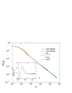
Figure 1: (Color online) Inter-communication time distribution in the 1d critical CP of size $N=10^{5}$. Full line denote histogramming from all times, dashed line from high times, long dashes from low times. The dotted line shows a power-law fit for $t>200$ resulting in $\propto t^{-1.85(5)}$. The solid thin line corresponds to runs from seed initial conditions. Inset: the same data multiplied by the $t^{1.85}$ corresponding to the tail decay.

The systems during the runs are in non-stationary state, hence the average $\Delta$ should increase getting close to extinction, still $P(\Delta)$ for finite sizes exhibits a power-law tail, characterized by $P(\Delta)\sim\Delta^{-x}$ with the exponent $x=1.85(5)$, obtained by least square fitting to the data. To check if the non-stationary would cause a change in $P(\Delta)$ the histogramming was performed for the early ($t\leq 5\times 10^{5}$ MCs) and late ($t>5\times 10^{5}$ MCs) events separately. One cannot see any differences, all three $P(\Delta)$ distributions exhibit power-law behavior. On the other hand the $P(\Delta)$ distributions above or below $\lambda_{c}$ show exponential tails as expected.

The scaling behavior at the critical point can be derived by expressing the inter-communication probability via the temporal auto-correlation function. Infection events can happen if there is an infected-uninfected neighbor pair, a kink in the spin language: $n_{i}(t)=1$, at site $i$ and time $t$. Using the two-time auto-correlation function $\Gamma(t,s)$ one can estimate the probability of the subsequent infection events, separated by a communication-free period $\Delta$ as:

$$P(\Delta)\simeq p^{2}\Gamma(t,s)\prod_{j=1}^{j<\Delta}[(1-p)\Gamma(j,s)+(1-\Gamma(j,s))]\simeq\Gamma(t,s)$$ (1)

using the connected temporal correlator between times $s$ and $t$

$$\Gamma(t,s)=\langle n_{i}(t)n_{i}(s)\rangle-\langle n_{i}(t)\rangle\langle n_{i}(s)\rangle$$ (2)

Here $\langle\rangle$ denotes averaging for independent runs. In this estimate the correlations among the inter-communication time events are neglected, however this does not affect the asymptotic behavior, because terms in the product are $\simeq O(1)$.

For 1d CP it is well known that this function exhibits an ageing behavior (see HDP ; Ódor (2008)), i.e. time translational invariance is broken, but in the $t,s\to\infty$ limit the densities $\langle n_{i}(t)\rangle\to 0$ and the correlator scales as

$$\Gamma(t,s)\propto(t/s)^{-\theta}=(\Delta/s+1)^{-\theta}$$ (3)

In case of 1d CP $\theta=1.80(5)$ (see HDP ; Ódor (2008)). This is also true for the kink variables, which also follow the same universal scaling behavior, belonging to the directed percolation class Ódor (2008). Strictly speaking due to the ageing behavior we have the scale dependence $P(t/s)\sim\Delta^{-\theta}$ and indeed the simulations confirm this (see Fig. 1). Asymptotically one can find the same leading order contribution for $P(\Delta)$, coming from the smallest $s$ in the statistical average and the tail behaviors agree with the auto-correlation function decay.

More generally, the site occupancy restriction condition of the CP is not a necessary condition to find fat inter-communication tails. One can easily deduce, that the power-law tail of $\Gamma(t,s)$ of infections causes also fat-tails of the link-activation inter-communication times. This has been confirmed by the simulations. Furthermore, simulation runs started from small activated seeds (see Ódor (2008)) resulted in the same tail in $P(\Delta)$ again (see Fig. 1), only the distribution of activation times changes. Contrary to the full initial condition case, where it decays as $\sim\Delta^{-0.16(1)}$ it increases as $\sim\Delta^{0.33(1)}$ in the case of seeds.

III Burstyness of the CP on generalized small-world networks

In this section I show results obtained for the CP on certain GSW networks BB . It has been shown that these system exhibit extended GP regions, with non-universal, $\lambda$ dependent power-law dynamics Muñoz et al. (2010); Juhász et al. (2011). The network generation starts with $N$ nodes on a ring. All nearest neighbors are connected with Euclidean distance $l=1$ with probability $1$ and pairs with $l>1$ with a probability $p(l)=1-\exp(-\beta l^{-s})$. For large distance this results in $p(l)\simeq\beta l^{-s}$. Now I consider the cases: $s=2$ with $\beta=0.1$ and $\beta=0.2$.

The inter-communication times of nodes were followed in networks with $L=10^{6}$ nodes up to $t_{max}=10^{6}$ MCs as in case of the pure CP. The number of independent samples at a given parameter, for which averaging was done, varied between $200$ and $1000$. The $P(\Delta)$ distributions were determined for several $\lambda$-s in the GP of these networks. Invariance of $P(\Delta)$ with respect to the measuring time windows has been checked, similarly to the pure critical CP case.

As Fig. 2 shows power-law tails emerge again, with slightly $\lambda$ dependent slopes for $\beta=0.1$ at $\lambda=2.97,3.02,3.07$ within the GP region of the model. To see dependency on $\lambda$ and the corrections to scaling I applied the standard local slope analysis (see Ódor (2008)) on the $P(\Delta)$ results. The effective exponent of $x$, which is the discretized, logarithmic derivative

$$x_{\mathrm{eff}}(t)=\frac{\ln P(\Delta)-\ln P(\Delta^{\prime})}{\ln(\Delta)-\ln(\Delta^{\prime})}\ ,$$ (4)

where $\Delta/\Delta^{\prime}=2$ difference was used here. As one can read-off from the inset of Fig. 2, at the critical point $\lambda_{c}=3.07(1)$, determined in Juhász et al. (2011), $x$ tends to $1.90(1)$ asymptotically as $\Delta\to\infty$. Below $\lambda_{c}$ the effective exponents converge to smaller values: $x=1.92(1)$ at $\lambda=3.02$ and $x=1.96(1)$ at $\lambda=2.97$. Corrections to the scaling are rather strong for $\Delta<5000$, but the effective exponents seem to saturate asymptotically. Note, that as in case of the density decay study of this model Juhász et al. (2011) logarithmic corrections were found in the GP.

As in case of the 1d CP the tail results are not affected by using an active initial seed condition or by measuring the times between the communication attempts of sites. The combined effect of this two modifications is shown on Fig. 2 for $\lambda_{c}=3.07$.

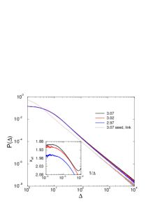
Figure 2: (Color online) Inter-communication time distribution in the GP of a GSW network with $\beta=0.1$ of size $N=10^{6}$ and $\lambda=2.97,3.02,3.07$ (bottom to top solid curves). The solid thin line corresponds to runs from seed initial conditions measuring all activation attempts. Inset: Effective exponents defined as (4) of the same data.

For $\beta=0.2$ one finds somewhat different power-law tails inside the GP (see Fig. 3). The local slope analysis suggests $x=1.94(1)$ at $\lambda_{c}=2.85$, $x=1.96(1)$ at $\lambda=2.8$ and $x=1.99(1)$ at $\lambda=2.75$. One can clearly see tail behaviors, characterized by increasing $x$ exponents with $\beta$, in agreement with the fact that the addition of long edges to the network increases the topological dimension, thus the auto-correlation exponent, which is $\theta=4$ in the mean-field limit.

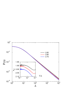
Figure 3: (Color online) Inter-communication time distribution in the GP of a GSW network with $\beta=0.2$ of size $N=10^{6}$ and $\lambda=2.75,2.8,2.85$ (bottom to top curves). Inset: Effective exponents defined as (4) of the same data.

IV Burstyness of the SIS model on ageing SF networks

In this section I show SIS model results on ageing SF networks, where cutting the links among highly connected nodes results in finite topological dimension and GP behavior basiscikk . In the original Barabási-Albert (BA)Barabási and Albert (1999) graph construction one starts from a single connected node and add new links with the linear preferential rule. In basiscikk I investigated a generalized model, in which fraction of edges of the ageing nodes were removed from the BA graph by a random, linear preferential rule. Consequently the edge distribution of the BA graph $P(k)\propto k^{-3}$ was cut off by an exponential factor for large $k$-s and quenched mean field theory suggested a GP behavior in agreement with the dynamical simulations.

SIS model density simulations were run on systems with $N=10^{5}$ nodes in the formerly determined GP region $2.4<\lambda<2.7$ of the ageing BA graphs basiscikk . Occurrence of fat tail $P(\Delta)$ distributions can be seen on Fig. 4, but now even network site ($i$-)dependency emerges. This is related to the fact that nodes are inhomogeneous: the average number of edges decreases as $\langle k_{i}\rangle\sim i^{-1/2}$ by the BA network generation. Least squares error power-law fitting for $\Delta>20$ leads to $\lambda$ and $i$ dependent decay exponents. For $\lambda=2.65$ and $i=1$, (highest connectivity node) the $P(\Delta)$ decay is characterized by the exponent $x=3.48(3)$, which is near to the mean-field value of the auto-correlation: $\theta=4$ of the CP. For less connected nodes ($i=100$) the decay is slower: $P(\Delta)\propto\Delta^{-2.96(3)}$, getting away from the mean-field value and coming closer to the one-dimensional auto-correlation exponent of CP. This agrees with that our expectations, since for larger $i$-s the connectivity decreases and the system exhibits auto-correlations of lower dimensionality. By decreasing $\lambda$ in the GP, as shown in Fig. 4 the following decreasing series of asymptotic tail exponents for $i=1$: $x=3.48(3),3.12(3),2.64(2),2.52(25),2.42(2)$. For $i=100$ at $\lambda=2.47$ the tail exponent is: $x=2.13(2)$. Again, logarithmic corrections to the dynamic scaling can also expected in the GP Vojta (2006).

To complete this study I also tested the critical point behavior of $P(\Delta)$ in case CP on the pure BA network (see BAGPcikk ) at $\lambda_{c}=1.21$. As the inset of Fig. 4 shows the tail behavior tends to a power-law with $x=4$ for $\Delta>20.000$ indeed.

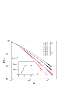
Figure 4: (Color online) Inter-communication time distribution in the GP of an ageing BA network of size $N=10^{5}$ for $\lambda=2.47,2.5,2.55,2.59,2.6,2.65$ (top to bottom curves) and measured at different ($i=1$ and $i=100$) sites. Power-law fitting exponents for the tail behavior is shown in the text. Inset: $P(\Delta)\Delta^{4}$ at the $\lambda_{c}$ of the CP defined on the pure BA graph.

V Dynamics of the CP and ARW on time varying networks

A simulation program has been created, with a fixed activity potential $F(V)\propto V^{-\gamma}$ attached to vertexes, such that two edges are connected to each node with that probability before each ’sweep’ of the network. One sweep (or Monte Carlo step) consists of $N$ random CP updates of the network of $N$ nodes. I followed $\rho(t)$ after a start from a fully occupied (infected) state. The time is updated by one MCs after a full network sweep. The simulations were run up to $t_{max}=2\times 10^{5}$ MCs on several sizes up to $N=10^{7}$ and repeated for $10^{2}-10^{3}$ independent randomly generated networks.

First $\gamma=3$ type of networks have been studied. The finite size effects are strong, but for large sizes ($N\sim 10^{7}$) a phase transition seems to appear with $\rho\propto 1/t$ decay, which agrees with the heterogeneous mean-field prediction BAGPcikk (see Fig. 5). Similar results have been found for $\gamma=2.8$ networks.

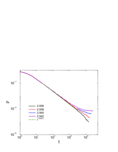
Figure 5: (Color online) Density decay of the Contact Process in time varying networks of sizes $N=10^{7}$ for $\lambda=2.936,2.938,2.940,2.942$ (bottom to top). The dashed line shows a power-law fit to the $\lambda=2.94$ (critical) curve. The activity potential decays with $\gamma=3$.

I have also tested the dynamical behavior of the Annihilating Random Walk (ARW) Ódor (2008) in networks with activity potential parameters: $\gamma=0.6,0.8,0.9,1,3.8$. The ARW model is a solvable model in homogeneous, Euclidean system, in which randomly selected particles hop to neighboring empty sites or annihilate with others on collision. In the high dimensional, mean-field limit the density of particles decays asymptotically as $t\propto 1/t$. As Fig. 6 shows simulations up to $t_{max}=10^{5}$ MCs with $N=10^{7}$ nodes result in the same asymptotic mean-field behavior following a long crossover time.

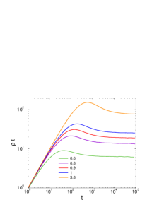
Figure 6: (Color online) Density decay in the ARW in time varying networks of sizes $N=10^{7}$ for $\gamma=0.6,0.8,0.9,1,3.8$ (bottom to top). The curves are the average of $10^{3}$ independent runs.

This suggests that slow, non-universal dynamics in activity driven time varying networks do not exists, strengthening the hypothesis Ódor et al. (2011) that quenched heterogeneity is a necessary condition for observing rare-region effects.

Not so surprisingly burstyness does not occur in such time varying networks either, because the network rewiring process destroys the long-range dynamical correlations. Simulations result in an exponential tail $P(\Delta)$ distributions.

VI Conclusions

Observed burstyness in network systems is assumed to be the related of the internal, non-Poissonian behavior of agents or state variables. This has been explained by different multi-level or time-scheduling internal models. In this paper I show an alternative route to this, being a natural consequence of correlated, complex behavior of the whole system. In case of the critical, one-dimensional Contact Process fat-tailed inter-communication time distribution arises, related to the diverging auto-correlation function.

Furthermore, the addition of long edges, which turns the network to GSWs with Griffiths Phases one can observe topology dependent, fat-tailed inter-communication time distributions.

I have also shown that in case of an ageing scale-free network, exhibiting Griffiths Phase these power-law distributions depend also on the average connectivity of nodes. The observed tail exponents vary in the range: $x=2-4$, which is smaller than the experimental values reported on human communication data-sets KKBK12 ; KKK12 . However, as the GSW model example shows there exist networks, possessing smaller topological dimensions, where $x<2$. Furthermore, there are other models HDP , like the bosonic contact process or the bosonic pair contact process, where the auto-correlation decays slower ($\theta=d/2$ for these unrestricted CPs BSH06 ), thus $x$ could also be smaller on networks.

It is important to note that these systems are in a non-stationary state during the simulations, still the tail distributions are time invariant and initial condition invariant. Usually real systems are also in the non-stationary state as the consequence of various external conditions, circadian oscillations. In case of regular networks the distributions are site invariant as well.

Finally I have shown that both the Contact Process and Annihilating Random Walks exhibit mean-field like dynamics on time varying, scale-free networks GP effects are absent and the distribution of inter-communication times is not bursty, but characterized by an exponential tail distribution.

These results suggest that bursty behavior can emerge as a collective behavior in quenched network systems close to criticality or in extended GP like regions, suggesting a closer inspection of such system. When real-world data confirms that sites exhibit inherent bursty behavior the superimpose of the two reason should emerge, possibly with the outcome of the more relevant one, which decays slower.

References

- Dorogovtsev et al. (2008) S. N. Dorogovtsev, A. V. Goltsev, and J. F. F. Mendes, Rev. Mod. Phys. 80, 1275 (2008).
- Barrat et al. (2008) A. Barrat, M. Barthélemy, and A. Vespignani, Dynamical Processes on Complex Networks (Cambridge University Press, Cambridge, 2008).
- (3) S. Johnson, J. J. Torres, and J. Marro, PLoS ONE 8(1): e50276 (2013)
- Pastor-Satorras and Vespignani (2001) R. Pastor-Satorras and A. Vespignani, Phys. Rev. Lett. 86, 3200 (2001).
- (5) R. Pastor-Satorras and A. Vespignani, Evolution and Structure of the Internet: A Statistical Physics Approach (Cambridge University, Cambridge, 2004).
- (6) M. Karsai et al. Phys. Rev. E 83 (2011) 025102(R)
- (7) A. Haimovici, E. Tagliazucchi, P. Balenzuela, and D. R. Chialvo, Phys. Rev. Lett. 110, 178101 (2013).
- (8) P. Moretti and M. Muñoz, Nature Communications 4, (2013) 2521
- (9) A.-L. Barab´asi, Bursts (Plume, 2010)
- (10) M. Karsai, K. Kaski, A.-L. Barabási, J. Kertész, Sci. Rep. 2, (2012) 397.
- (11) M. Karsai, K. Kaski, J. Kertész, PLoS ONE 7 e40612 (2012)
- (12) C. Cattuto, W. V. den Broeck, A. Barrat, V. Colizza, J.-F. Pinton, and A. Vespignani, PLoS ONE 5, e11596 (2010).
- (13) J. Kleinberg, Data Mining and Knowledge Discovery 7, 373 (2003)
- (14) J.-P. Eckmann, E. Moses, D. Sergi, Proc. Natl. Acad. Sci. 101, 14333 (2004)
- (15) A.-L. Barab´asi, Nature 435, 207 (2005)
- Griffiths (1969) R. B. Griffiths, Phys. Rev. Lett. 23, 17 (1969).
- Vojta (2006) T. Vojta, Journal of Physics A: Mathematical and General 39, R143 (2006).
- Muñoz et al. (2010) M. A. Muñoz, R. Juhász, C. Castellano, and G. Ódor, Phys. Rev. Lett. 105, 128701 (2010).
- Ódor et al. (2011) G. Ódor, R. Juhasz, C. Castellano, and M. A. Munoz, in Nonequilibrium Statistical Physics Today, Vol. 1332, edited by P. L. Garrido, J. Marro, and F. de los Santos (AIP, 2011) pp. 172–178.
- Juhász et al. (2011) R. Juhász, G. Ódor, C. Castellano, and M. A. Muñoz, Phys. Rev. E. 85, 066125 (2012).
- (21) G.Ódor and R. Pastor-Satorras, Phys. Rev. E 86, (2012) 026117.
- (22) G.Ódor, Phys. Rev. E 87, (2013) 042132.
- (23) G.Ódor, Phys. Rev. E 88, (2013) 032109.
- (24) C. Monthus, T. Garel, J. Phys. A: Math. Theor. 44 (2011) 085001.
- (25) I. A. Kovács and F. Iglói, J. Phys.: Condens. Matter 23, 404204 (2011).
- (26) R. Juhász and I. A. Kovács, J. Stat. Mech. (2013) P06003.
- Harris (1974a) T. E. Harris, Ann. Prob. 2, 969 (1974a).
- Liggett (1985) T. M. Liggett, Interacting Particle Systems (Springer-Verlag, New York, 1985).
- (29) P. Erdős and A. Rényi, A. (1959) Publ. Math. 6, 290–291.
- (30) M. Aizenman and C.M. Newman, Commun. Math. Phys. 107, 611 (1986).
- (31) R. Juhász, Phys. Rev. E 78, 066106 (2008).
- (32) R. Juhász, G. Ódor, Phys. Rev. E 80, 041123 (2009).
- (33) R. M. Anderson and R. M. May, Infectious diseases in humans, (Oxford University Press, Oxford, 1992).
- (34) R. Lambiotte, L. Tabourier and J.-C. Delvenne, Eur. Phys. J. B (2013) 86 320.
- Marro and Dickman (1999) J. Marro and R. Dickman, Nonequilibrium Phase Transitions in Lattice Models (Cambridge University Press, Cambridge, 1999).
- (36) G. Ódor, Rev. Mod. Phys. 76 (2004) 663
- Ódor (2008) G. Ódor, Universality in Nonequilibrium Lattice Systems (World Scientific, Singapore, 2008).
- (38) M. Henkel, H. Hinrichsen and S. Lübeck, Non-Equilibrium Phase Transitions vol. 1., Springer 2008
- (39) M. Henkel and M. Pleimling, Non-equilibrium phase transitions,vol 2: Ageing and dynamical scaling far from equilibrium, Springer (Heidelberg 2010).
- (40) N. Perra, B. Goncalves, R. Pastor-Satorras and A. Vespignani, Nature Scientific Reports 2, 469 (2012).
- (41) I. Benjamini and N. Berger, Rand. Struct. Alg. 19, 102 (2001).
- (42) F. Baumann, S. Stoimenov and M. Henkel, J. Phys. A: Math. Gen. 39 (2006) 4095–4118
- Barabási and Albert (1999) A.-L. Barabási and R. Albert, Science 286, 509 (1999).