How to suppress the backscattering of conduction electrons?

Abstract

It is shown theoretically that the strong coupling of electrons to a high-frequency electromagnetic field results in the nulling of electron backscattering within the Born approximation. The conditions of the effect depend only on field parameters and do not depend on concrete form of scattering potential. As a consequence, this phenomenon is of universal physical nature and can take place in various conducting systems. Since the suppression of electron backscattering results in decreasing electrical resistance, the solved quantum-mechanical problem opens a new way to control electronic transport properties of conductors by a laser-generated field. Particularly, the elaborated theory is applicable to nanostructures exposed to a strong monochromatic electromagnetic wave.

1 Introduction

The backscattering is fundamental physical process consisting in the reflection of moving electrons back to the direction from which they came. Resulting in dissipation of kinetic momentum of the electrons, the backscattering lies in the core of all mechanisms of electrical resistance in conductors. Therefore, the seeking for ways to suppress the backscattering is problem of both general physical interest and rich applied capabilities. In the given Letter, it is shown theoretically how the backscattering of conduction electrons can be suppressed by a high-frequency electromagnetic field.

Due to advances in laser physics, a strong electromagnetic field became an ordinary tool to manipulate electronic properties of various systems. In contrast to the case of weak electromagnetic field, the interaction between electrons and the strong field cannot be described as a perturbation. Therefore, the system “electron + strong electromagnetic field” should be considered as a bound electron-field object which was called “electron dressed by field” (dressed electron) [1, 2]. In atomic and molecular systems, the interaction between electrons and a dressing field results in various phenomena, including both the photon-induced modification of electron energy spectrum (the dynamic Stark effect) [3, 4, 5, 6, 7] and the photon-assisted scattering of electrons by atoms and molecules [8, 9, 10, 11, 12]. In condensed matters, research activity was focused on the dynamic Stark effect [13, 14, 15, 16, 17, 18, 19, 20, 21, 22, 23, 24, 25, 26] and the photon-assisted non-stationary quantum transport through potential barriers [27, 28, 29, 30]. As to effect of dressing field on scattering processes which are responsible for stationary (dc) electronic transport in usual conducting systems, it escaped attention before. Filling this gap in the theory, I unexpectedly found that the modification of electron wave functions by a strong high-frequency electromagnetic field results in the nulling of scattering matrix elements. As a consequence, the phenomenon announced above appears. Surprisingly, this quantum effect can be derived directly from the basic principles of quantum mechanics with using simple pen-and-paper calculations as follows.

2 The model

For definiteness, we will restrict our consideration by the case of alternating homogeneous electric field but the proper generalization for any electromagnetic field can be easily made. Let an electron be subjected to such an electric field

$$\mathbf{E}(t)=\mathbf{E}_{0}\sin\omega t,$$ (1)

where $E_{0}$ is the amplitude of the field, and $\omega$ is the frequency of the field. In the absence of scatterers, the wave function of the electron, $\psi$, satisfies the Schrödinger equation

$$i\hbar\frac{\partial\psi}{\partial t}=\hat{\cal{H}}_{0}\psi$$ (2)

with the Hamiltonian

$$\hat{\cal{H}}_{0}=\frac{1}{2m}\left[\hat{\mathbf{p}}-\frac{e}{c}\mathbf{A}(t)\right]^{2},$$ (3)

where $\hat{\mathbf{p}}$ is the operator of electron momentum, $m$ is the effective electron mass in a conductor, $e$ is the electron charge,

$$\mathbf{A}(t)=\frac{c\mathbf{E}_{0}}{\omega}\cos\omega t$$ (4)

is the vector potential of the field, and the field frequency $\omega$ is assumed to be far from resonant electron frequencies corresponding to interband electron transitions in the conductor. It should be noted that the Hamiltonian (3) with the same vector potential (4) describes a two-dimensional (or one-dimensional) electron system subjected to a plane linearly polarized monochromatic electromagnetic wave with the frequency $\omega$ and the amplitude $E_{0}$, which propagates perpendicularly to the system. As a consequence, the theory developed below is applicable, particularly, to such nanostructures as quantum wells and quantum wires exposed to the electromagnetic wave.

Since the vector potential (4) does not depend on coordinates, the nonstationary Schrödinger equation (2) with the Hamiltonian (3) can be solved accurately. Namely, let us seek the wave function $\psi$ in the form

$$\psi=V^{-1/2}\exp\left[-iF(t)-i\mathbf{k}\mathbf{r}\right],$$ (5)

where $\mathbf{k}$ is the electron wave vector, $\mathbf{r}$ is the electron radius-vector, $V$ is the normalization volume, and $F(t)$ is the required function. Substituting the wave function (5) into the Schrödinger equation (2), we arrive at the differential equation,

$$\hbar\frac{dF(t)}{dt}=\frac{\hbar^{2}\mathbf{k}^{2}}{2m}-\frac{\hbar e}{mc}\mathbf{k}\mathbf{A}(t)+\frac{e^{2}}{2mc^{2}}\mathbf{A}^{2}(t),$$

which can be easily solved by direct integration over time $t$. As a result, the exact wave function of the dressed electron (5) can be written as

$$\psi_{\mathbf{k}}(\mathbf{r},t) = \exp\left[-i\left(\frac{\varepsilon_{k}t}{\hbar}+\frac{E_{0}^{2}e^{2}t}{4m\omega^{2}\hbar}+\frac{E_{0}^{2}e^{2}}{8m\omega^{3}\hbar}\sin 2\omega t\right.\right.$$ (6)

$$- \left.\left.\frac{e\mathbf{E}_{0}\mathbf{k}}{m\omega^{2}}\sin\omega t\right)\right]\varphi_{\mathbf{k}}(\mathbf{r}),$$

where $\varphi_{\mathbf{k}}(\mathbf{r})={V}^{-1/2}\exp(i\mathbf{k}\mathbf{r})$ is the plane electron wave, and $\varepsilon_{k}={\hbar^{2}k^{2}}/{2m}$ is the energy spectrum of bare electron. As expected, in the absence of the field ($E_{0}=0$) the wave function of dressed electron (6) turns into the wave function of bare electron,

$$\psi_{\mathbf{k}}^{(0)}(\mathbf{r},t)=\varphi_{\mathbf{k}}(\mathbf{r})\exp(-i\varepsilon_{k}t/\hbar).$$ (7)

It should be stressed that the velocity of the dressed electron averaged over the field period $T=2\pi/\omega$,

$$\mathbf{v}(\mathbf{k})=\frac{1}{T}\int_{0}^{T}\left\langle\psi_{\mathbf{k}}(\mathbf{r},t)\left|\frac{\hat{\mathbf{p}}-e\mathbf{A}(t)/c}{m}\right|\psi_{\mathbf{k}}(\mathbf{r},t)\right\rangle dt=\frac{\hbar\mathbf{k}}{m},$$

exactly coincides with the stationary velocity of bare electron in the state (7) with the same wave vector $\mathbf{k}$,

$$\mathbf{v}^{(0)}(\mathbf{k})=\left\langle\psi_{\mathbf{k}}^{(0)}(\mathbf{r},t)\left|\frac{\hat{\mathbf{p}}}{m}\right|\psi_{\mathbf{k}}^{(0)}(\mathbf{r},t)\right\rangle=\frac{\hbar\mathbf{k}}{m}.$$

Thus, the high-frequency field does not change the mean electron velocity and, correspondingly, does not influence directly on stationary (dc) electronic transport. However, the formal mathematical difference between the wave function of dressed electron (6) and the wave function of bare electron (7) effects on scattering processes discussed below.

Let an electron moves in a conductor with scatterers in the presence of the same field (4). Then the wave function of the conduction electron, $\Psi(\mathbf{r},t)$, satisfies the Schrödinger equation

$$i\hbar\frac{\partial\Psi(\mathbf{r},t)}{\partial t}=[\hat{\cal H}_{0}+U(\mathbf{r})]\Psi(\mathbf{r},t),$$ (8)

where the total scattering potential $U(\mathbf{r})$ is superposition of potentials arisen from macroscopically large number of scatterers in the conductor. In what follows, we will assume the scattering potential energy $U(\mathbf{r})$ to be a small perturbation. This allows to apply the conventional perturbation theory [31] to describe the electron scattering by the potential $U(\mathbf{r})$. Since the functions (6) with different wave vectors $\mathbf{k}$ form the complete function system for any time $t$, we can seek solutions of the Schrödinger equation (8) as an expansion

$$\Psi(\mathbf{r},t)=\sum_{\mathbf{k}^{\prime}}a_{\mathbf{k}^{\prime}}(t)\psi_{\mathbf{k}^{\prime}}(\mathbf{r},t).$$ (9)

It should be stressed that eq. (6) gives exact wave functions of dressed electron. Therefore, the using of the basis (6) in the expansion (9) takes into account the interaction between an electron and the dressing field (4) in full, i.e. non-perturbatively. Let an electron be in the state (6) with the wave vector $\mathbf{k}$ at the time $t=0$. Correspondingly, $a_{\mathbf{k}^{\prime}}(0)=\delta_{\mathbf{k}^{\prime},\mathbf{k}}$, where $\delta_{\mathbf{k}^{\prime},\mathbf{k}}$ is the Kronecker symbol. Substituting the expansion (9) into the Schrödinger equation (8) and restricting the accuracy by the first order of the perturbation theory, we arrive at the expression

$$a_{\mathbf{k}^{\prime}}(t)=-i\frac{U_{\mathbf{k}^{\prime}\mathbf{k}}}{\hbar}\int_{0}^{t}e^{i(\varepsilon_{k^{\prime}}-\varepsilon_{k})t^{\prime}/{\hbar}}e^{if_{\mathbf{k}^{\prime}\mathbf{k}}\sin\omega t^{\prime}}dt^{\prime},$$ (10)

where $\mathbf{k}^{\prime}\neq\mathbf{k}$,

$$U_{\mathbf{k}^{\prime}\mathbf{k}}=\left\langle\varphi_{\mathbf{k}^{\prime}}(\mathbf{r})\left|U(\mathbf{r})\right|\varphi_{\mathbf{k}}(\mathbf{r})\right\rangle$$ (11)

is the matrix element of the scattering potential, and

$$f_{\mathbf{k}^{\prime}\mathbf{k}}=\frac{e\mathbf{E}_{0}(\mathbf{k}-\mathbf{k}^{\prime})}{m\omega^{2}}.$$ (12)

To proceed analysis of the problem, we have to slightly extend the conventional perturbation theory [31] which was developed by Dirac for stationary basis wave functions, taking into account the non-stationarity of the wave functions (6). Namely, let us apply the Jacobi-Anger expansion [32],

$$e^{iz\sin\theta}=\sum_{n=-\infty}^{\infty}J_{n}(z)e^{in\theta},$$

in order to rewrite eq. (10) as

$$|a_{\mathbf{k}^{\prime}}(t)|^{2} = \frac{\left|U_{\mathbf{k}^{\prime}\mathbf{k}}\right|^{2}}{\hbar^{2}}\Bigg{|}\sum_{n=-\infty}^{\infty}{J_{n}\left(f_{\mathbf{k}^{\prime}\mathbf{k}}\right)}\,e^{i(\varepsilon_{k^{\prime}}-\varepsilon_{k}+n\hbar\omega)t/{2\hbar}}$$ (13)

$$\times \int_{-t/2}^{t/2}e^{i(\varepsilon_{k^{\prime}}-\varepsilon_{k}+n\hbar\omega)t^{\prime}/\hbar}dt^{\prime}\Bigg{|}^{2},$$

where $J_{n}(z)$ is the Bessel function of the first kind. Since the integrals in eq. (13) for long time $t$ turn into the delta-function

$$\delta(\varepsilon)=\frac{1}{2\pi\hbar}\lim_{t\rightarrow\infty}\int_{-t/2}^{t/2}e^{i\varepsilon t^{\prime}/\hbar}dt^{\prime},$$

the expression (13) takes the form

$$|a_{\mathbf{k}^{\prime}}(t)|^{2}=4\pi^{2}\left|U_{\mathbf{k}^{\prime}\mathbf{k}}\right|^{2}\sum_{n=-\infty}^{\infty}J_{n}^{2}\left(f_{\mathbf{k}^{\prime}\mathbf{k}}\right)\delta^{2}(\varepsilon_{k^{\prime}}-\varepsilon_{k}+n\hbar\omega).$$ (14)

To transform square delta-functions in eq. (14), we can apply the conventional procedure (see, e.g., ref. [33]),

$$\delta^{2}(\varepsilon)=\delta(\varepsilon)\delta(0)=\frac{\delta(\varepsilon)}{2\pi\hbar}\lim_{t\rightarrow\infty}\int_{-t/2}^{t/2}e^{i0\times t^{\prime}/\hbar}dt^{\prime}=\frac{\delta(\varepsilon)t}{2\pi\hbar}.$$

Then the probability of the electron scattering between the states (6) with the wave vectors $\mathbf{k}$ and $\mathbf{k}^{\prime}$ per unit time, $w_{\mathbf{k}^{\prime}\mathbf{k}}=d|a_{\mathbf{k}^{\prime}}(t)|^{2}/dt$, is given by

$$w_{\mathbf{k}^{\prime}\mathbf{k}}=\frac{2\pi}{\hbar}\left|U_{\mathbf{k}^{\prime}\mathbf{k}}\right|^{2}\sum_{n=-\infty}^{\infty}J_{n}^{2}\left(f_{\mathbf{k}^{\prime}\mathbf{k}}\right)\delta(\varepsilon_{k^{\prime}}-\varepsilon_{k}+n\hbar\omega).$$ (15)

3 Results

The announced effect follows from the fact that all terms in the probability (15) can be nulled with a strong high-frequency field. First of all, let us consider the terms with $n\neq 0$. Physically, they describe the processes of collisional (intraband) absorption and emission of photons by conduction electron. Within the classical Drude theory, the collisional absorption of the field (1) by conduction electrons is given by the well-known expression

$$Q=\frac{1}{T}\int_{0}^{T}\mathbf{j}(t)\mathbf{E}(t)dt=\frac{E_{0}^{2}}{2}\frac{\sigma_{0}}{1+(\omega\tau)^{2}},$$ (16)

where $Q$ is the period-averaged field energy absorbed by conduction electrons per unit time and per unit volume, $\mathbf{j}(t)$ is the ohmic current density induced by the high-frequency field $\mathbf{E}(t)$, $\sigma_{0}=e^{2}n\tau/m$ is the static Drude conductivity, $n$ is the density of conduction electrons, and $\tau$ is the electron relaxation time (see, e.g., Refs. [34, 35]). Evidently, the Drude optical absorption (16) is negligibly small under the condition

$$\omega\tau\gg 1.$$ (17)

Therefore, it it reasonable to expect that terms with $n\neq 0$ in eq. (15), which describe the same optical absorption from the quantum point of view, are also negligibly small under the condition (17).

Within quantum theory, the absence of energy exchange between conduction electrons and a high-frequency electromagnetic field follows directly from the conservation laws. Namely, it is well-known that the conservation laws for energy and momentum forbid the processes of intraband absorption and emission of photons by conduction electrons. These processes are appreciable only if the scattering-induced washing of electron energy, $\delta\varepsilon$, is comparable with the photon energy $\hbar\omega$. As a consequence, the terms with $n\neq 0$ in eq. (15) can be neglected if the field frequency $\omega$ is high to satisfy the condition $\hbar\omega\gg\delta\varepsilon$. Applying the uncertainty relation for energy, $\delta\varepsilon\sim\hbar/\tau$, to this condition, we arrive again at the inequality (17).

The simple arguments based on the conservation laws can be verified formally by analysis of the Schrödinger equation. Namely, we have to consider the Hamiltonian $\hat{\cal H}=\hat{\mathbf{p}}/2m+U(\mathbf{r})$ describing a conduction electron in a scattering potential $U(\mathbf{r})$ in the absence of the field. The stationary Schrödinger equation with the Hamiltonian, $\hat{\cal H}u_{l}(\mathbf{r})=\varepsilon_{l}u_{l}(\mathbf{r})$, yields the energy spectrum $\varepsilon_{l}$ and the wave functions $u_{l}(\mathbf{r})$ of the electron, where the index $l$ labels various eigenstates of the Hamiltonian. Since the stationary eigenfunctions $u_{l}(\mathbf{r})$ form the complete function system, the wave function of free conduction electron, $\varphi_{\mathbf{k}}(\mathbf{r})=V^{-1/2}\exp(i\mathbf{k}\mathbf{r})$, can be expanded on the eigenfunctions as $\varphi_{\mathbf{k}}(\mathbf{r})=\sum_{l}b_{\mathbf{k}l}u_{l}(\mathbf{r})$. Then the matrix element (11) is

$$U_{\mathbf{k}^{\prime}\mathbf{k}}=\left\langle\varphi_{\mathbf{k}^{\prime}}(\mathbf{r})\left|\hat{\cal H}\right|\varphi_{\mathbf{k}}(\mathbf{r})\right\rangle=\sum_{l}\varepsilon_{l}b^{\ast}_{\mathbf{k}^{\prime}l}b_{\mathbf{k}l}.$$ (18)

Physically, the expansion coefficients $b_{\mathbf{k}l}$ describe the broadening of energy spectrum of conduction electron caused by the scattering: An electron with the wave vector $\mathbf{k}$ has the non-zero probability $W_{\mathbf{k}l}=|b_{\mathbf{k}l}|^{2}$ to be in the eigenstate $l$ with the energy $\varepsilon_{l}$. If to rewrite the coefficients as $b_{\mathbf{k}l}=\sqrt{W_{\mathbf{k}^{\prime}l}}e^{i\phi_{kl}}$, the matrix element (18) takes the form

$$U_{\mathbf{k}^{\prime}\mathbf{k}}=\sum_{l}\varepsilon_{l}\sqrt{W_{\mathbf{k}^{\prime}l}W_{\mathbf{k}l}}e^{i(\phi_{kl}-\phi_{k^{\prime}l})}.$$ (19)

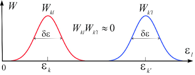
Figure 1: Scheme of the scattering-induced washing of electron states $\varepsilon_{k}$ and $\varepsilon_{k^{\prime}}$ in a conductor. The overlap of the plotted probabilities $W_{kl}$ and $W_{k^{\prime}l}$ — and, correspondingly, the product $W_{kl}W_{k^{\prime}l}$ — is negligibly small under the condition $|\varepsilon_{k}-\varepsilon_{k^{\prime}}|\gg\delta\varepsilon$.

The scattering-induced washing of electron energy, $\delta\varepsilon$, is the energy range near the energy of free electron, $\varepsilon_{k}={\hbar^{2}k^{2}}/{2m}$, where the probability $W_{\mathbf{k}l}$ distinctly differs from zero (see fig. 1). Therefore, the product $W_{\mathbf{k}^{\prime}l}W_{\mathbf{k}l}$ — and, correspondingly, the sum in eq. (19) — is very small under the condition $|\varepsilon_{k}-\varepsilon_{k^{\prime}}|\gg\delta\varepsilon$. As a consequence, the matrix element (19) is negligibly small in those terms of eq. (15), which satisfy this condition. Since the terms with $n\neq 0$ in eq. (15) describe the electron scattering between the states $\mathbf{k}$ and $\mathbf{k}^{\prime}$ with the energy difference $|\varepsilon_{k}-\varepsilon_{k^{\prime}}|\geq\hbar\omega$, these terms are very small for $\hbar\omega\gg\delta\varepsilon$. Therefore, they can be neglected if $\hbar\omega\gg\delta\varepsilon$. Taking into account the uncertainty relation for energy, $\delta\varepsilon\sim\hbar/\tau$, this condition can be rewritten in the form (17). Thus, both classical and quantum description of the problem lead to the same result: The collisional absorption (emission) of field energy by conduction electrons can be neglected if the field frequency $\omega$ is high enough.

Assuming the condition (17) to be satisfied, we can omit terms with $n\neq 0$ in eq. (15). Then the probability of electron scattering (15) takes the final form

$$w_{\mathbf{k}^{\prime}\mathbf{k}}=\frac{2\pi}{\hbar}J_{0}^{2}\left(f_{\mathbf{k}^{\prime}\mathbf{k}}\right)\left|U_{\mathbf{k}^{\prime}\mathbf{k}}\right|^{2}\delta(\varepsilon_{k^{\prime}}-\varepsilon_{k}).$$ (20)

The formal difference between the scattering probability of dressed electron (20) and the conventional expression for the scattering probability of bare electron [31],

$$w^{(0)}_{\mathbf{k}^{\prime}\mathbf{k}}=\frac{2\pi}{\hbar}\left|U_{\mathbf{k}^{\prime}\mathbf{k}}\right|^{2}\delta(\varepsilon_{k^{\prime}}-\varepsilon_{k}),$$ (21)

consists in the Bessel-function factor $J_{0}^{2}\left(f_{\mathbf{k}^{\prime}\mathbf{k}}\right)$, where $f_{\mathbf{k}^{\prime}\mathbf{k}}$ is proportional to the field amplitude $E_{0}$ [see eq.(12)]. This factor arises from the strong electron coupling to the field: If the field is absent ($E_{0}=0$), this factor is equal to unity and, as expected, the expressions (20) and (21) coincide. However, for $E_{0}\neq 0$ just this factor leads to the effect announced above. Namely, it follows from the oscillatory behavior of the Bessel function that there are amplitudes of the field, $E_{0}$, for which the Bessel function $J_{0}(f_{\mathbf{k}^{\prime}\mathbf{k}})$ is null. As a consequence, the field can turn the probability of scattering (20) into zero. Particularly, eq. (20) describes the probability of electron backscattering if $\mathbf{k}^{\prime}=-\mathbf{k}$. This probability,

$$W=\frac{w_{-\mathbf{k}\mathbf{k}}}{w^{(0)}_{-\mathbf{k}\mathbf{k}}}=J^{2}_{0}\left(\frac{2e\mathbf{E}_{0}\mathbf{k}}{m\omega^{2}}\right),$$ (22)

is qualitatively pictured in fig. 2 as a function of the field amplitude $E_{0}$. Evidently, the backscattering is absent for the field amplitudes $E_{0}$ satisfying the equation

$$J_{0}\left(\frac{2e\mathbf{E}_{0}\mathbf{k}}{m\omega^{2}}\right)=0$$ (23)

which gives nulls of the probability (22).

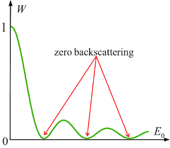
Figure 2: The probability of backscattering of a dressed electron as a function of amplitude of dressing field.

4 Discussion and conclusions

It should be noted that the expression (20) describes the probability of electron scattering within the main (first) order of the perturbation theory, which corresponds to the Born approximation [31]. As a consequence, the nulling of the probability (20) suppresses the backscattering effectively if the scattering potential $U(\mathbf{r})$ meets the well-known conditions of applicability of this approximation [31]. These conditions cover a lot of physical situations which can be experimentally realized in various conducting systems. Particularly, the scattering of conduction electrons in modern nanostructures arises from a very weak scattering potential $U(\mathbf{r})$ and can be described by the theory elaborated above. However, it can be useful for possible experiments to estimate the remanent backscattering arisen from the second order of the perturbation theory. Going in the same way as before, one can derive the second-order probability of the electron scattering,

$$w_{\mathbf{k}^{\prime}\mathbf{k}} = \frac{2\pi}{\hbar}\left|\sum_{\mathbf{k}^{\prime\prime}}J_{0}\left(f_{\mathbf{k}^{\prime}\mathbf{k}^{\prime\prime}}\right)J_{0}\left(f_{\mathbf{k}^{\prime\prime}\mathbf{k}}\right)\frac{U_{\mathbf{k}^{\prime}\mathbf{k}^{\prime\prime}}U_{\mathbf{k}^{\prime\prime}\mathbf{k}}}{\varepsilon_{k}-\varepsilon_{k^{\prime\prime}}}\right|^{2}$$ (24)

$$\times \delta(\varepsilon_{k^{\prime}}-\varepsilon_{k}),$$

which describes the remanent scattering in the high-frequency limit if the main scattering (20) is nulled by a dressing field. As expected, the probability (24) is negligibly small under the conditions of the Born approximation [31].

Replacing the scattering probability of bare electron (21) with the scattering probability of dressed electron (20) in the conventional kinetic Boltzmann equation for conduction electrons (see, e.g., ref. [36]), one can calculate stationary (dc) transport properties of dressed electrons. Particularly, the discussed suppression of the electron backscattering leads to increasing electron mobility. Applying a stationary voltage to a conducting system dressed by a strong high-frequency electromagnetic field, the field-induced decreasing of electrical resistance can be measured experimentally. It should be stressed that the probability (20) describes an elastic scattering of dressed electron. However, in conducting systems there are various mechanisms of electron scattering, including both elastic scattering processes arisen from impurities and unelastic ones caused by phonons. Therefore, the given theory can accurately describe transport properties of dressed electrons if the elastic scattering is dominant. This always takes place if temperature is low enough.

The discussed effect is caused by nonlinear electron interaction with a strong electromagnetic field. Mathematically, this follows from the key expression (23), where the field amplitude $E_{0}$ takes place in argument of highly nonlinear Bessel function. Therefore, the effect under consideration cannot be derived from the usual treatment of the problem, which is based on expansion of the kinetic Boltzmann equation in a power series of field amplitude. It should be noted also that the condition (17) requires a high field frequency $\omega$. On the other hand, if the frequency $\omega$ is very high, the condition (23) can be realized only for very high field amplitudes $E_{0}$. Since high field amplitudes correspond to high field intensities, strong fields satisfying both the condition (17) and the condition (23) can fluidize a conductor. To avoid fusion of experimental samples, one needs to use conductors with high electron mobility (for instance, modern nanostructures), where the conditions (17) and (23) can be satisfied for low field intensities.

Though the effect under consideration is of general character, it will be most pronounced in one-dimensional nanostructures (for instance, in semiconductor quantum wires, carbon nanotubes, etc) since the backscattering is the only mechanism restricting the mean free path of conduction electrons there. It should be noted also that low-dimensional conductors are most preferable from experimental viewpoint due to the absence of the screening of dressing electromagnetic field. Therefore, let us estimate observability of the discussed effect for conduction electrons in one-dimensional conductors (for definiteness, in semiconductor quantum wires with the effective electron mass $m\sim 10^{-29}$ g). For such conductors, the modern nanotechnologies allow to reach the electron mobility $\mu=e\tau/m\sim 10^{7}$ cm${}^{2}/$V$\cdot$s that corresponds to the electron relaxation time $\tau\sim 10^{-9}$ s. Therefore, the condition (17) can be satisfied for the field frequencies $\omega\geq 10^{10}$ Hz. Let the wire be filled by a degenerate electron gas with the Fermi energy $\varepsilon_{F}=\hbar^{2}k^{2}_{F}/2m\sim 10^{-2}$ eV that corresponds to the Fermi electron wave vector $k_{F}\sim 10^{6}$ cm^-1. Assuming the wire to be exposed to a high-frequency field (1) directed along the wire, the condition (23) can be satisfied for the Fermi electrons if the field amplitude is $E_{0}\geq 10^{2}$ V/m. This field amplitude corresponds to the field intensity $I\geq 10^{-3}$ W/cm². Thus, the suppression of electron backscattering can be realized for experimentally reasonable parameters of the field. Finalizing the discussion, another experimental consequence of this effect should be noted: Since the factor $J_{0}^{2}\left(f_{\mathbf{k}^{\prime}\mathbf{k}}\right)$ in the scattering probability (20) is the oscillating function of the field amplitude $E_{0}$ (see fig. 2), all stationary electronic transport characteristics of field-dressed conductors are expected to oscillate in the same manner.

Summarizing the aforesaid, the novel quantum effect — the nulling of the Born backscattering caused by a high-frequency electromagnetic field — is claimed. It should be stressed that the conditions of the effect (17) and (23) depend only on field parameters and do not depend on concrete form of the scattering potential. Thus, always there is an electromagnetic field resulting in the nulling. As a consequence, the effect is of universal physical nature. Since the suppression of electron backscattering results in decreasing electrical resistance, the solved quantum-mechanical problem opens an unexplored way to control electronic transport properties of conductors and electronic devices by a high-frequency electromagnetic field. Particularly, the elaborated theory is applicable to nanostructures exposed to a strong monochromatic electromagnetic wave.

5 Acknowledgements

The work was partially supported by the Russian Ministry of Education and Science, RFBR (projects No. 13-02-90600 and No. 14-02-00033) and FP7 project QOCaN.

References

- [1] \NameCohen-Tannoudji C., Dupont-Roc J. Grynberg G. \BookAtom-Photon Interactions: Basic Processes and Applications \PublWiley, Chichester \Year1998.
- [2] \NameScully M. O. Zubairy M. S. \BookQuantum Optics \PublUniversity Press, Cambridge \Year2001.
- [3] \NameAutler S. H. Townes C. H. \REVIEWPhys. Rev.1001955703.
- [4] \NameChini M., Zhao B., Wang H., Cheng Y., Hu S. X. Chang Z. \REVIEWPhys. Rev. Lett.1092012073601.
- [5] \NameYu C., Fu N., Hu T., Zhang G. Yao J. \REVIEWPhys. Rev. Lett.882013043408.
- [6] \NameDemekhin P. V. Cederbaum L. S. \REVIEWPhys. Rev. A882013043414.
- [7] \NameGiner L., Veissier L., Sparkes B., Sheremet A. S., Nicolas A., Mishina O. S., Scherman M., Burks S., Shomroni I., Kupriyanov D. V., Lam P. K., Giacobino E. Laurat J. \REVIEWPhys. Rev. A872013013823.
- [8] \NameBunkin V. F. Fedorov M. V. \REVIEWJETP221969844.
- [9] \NameKroll N. M. Watson K. M. \REVIEWPhys. Rev. A81973 804.
- [10] \NameKanya R., Morimoto Y. Yamanouchi K. \REVIEWPhys. Rev. Lett.1052010123202.
- [11] \NameBhatia A. K. Sinha C. \REVIEWPhys. Rev. A862012 053421.
- [12] \NameFlegel A. V., Frolov M. V., Manakov N. L., Starace A. F. Zheltukhin A. N. \REVIEWPhys. Rev. A872013013404.
- [13] \NameGoreslavskii S. P. Elesin V. F. \REVIEWJETP Lett.101969316.
- [14] \NameMysyrowicz A., Hulin D., Antonetti A., Migus A., Masselink W. Y. Morkoç H. \REVIEWPhys. Rev. Lett.5619862748.
- [15] \NameLindberg M. Koch S. W. \REVIEWPhys. Rev. B3819887607.
- [16] \NameVu Q. T., Haug H., Mücke O. D., Tritschler T., Wegener M., Khitrova G. Gibbs H. M. \REVIEWPhys. Rev. Lett.922004217403.
- [17] \NameDynes J. F., Frogley M. D., Beck M., Faist J. Phillips C. C. \REVIEWPhys. Rev. Lett.942005157403.
- [18] \NameLópez-Rodríguez F. G. Naumis G. G. \REVIEWPhys. Rev. B782008201406(R).
- [19] \NameKibis O. V., Slepyan G. Ya., Maksimenko S. A. Hoffmann A. \REVIEWPhys. Rev. Lett.1022009023601.
- [20] \NameKibis O. V. \REVIEWPhys. Rev. B812010165433.
- [21] \NameKibis O. V. \REVIEWPhys. Rev. Lett.1072011106802.
- [22] \NameSavel’ev S. E. Alexandrov A. S. \REVIEWPhys. Rev. B842011035428.
- [23] \NameKibis O. V., Kyriienko O. Shelykh I. A. \REVIEWPhys. Rev. B842011195413.
- [24] \NameKibis O. V. \REVIEWPhys. Rev. B862012155108.
- [25] \NameHayat A., Lange C., Rozema L. A., Darabi A., van Driel H. M., Steinberg A. M., Nelsen B., Snoke D. W., Pfeiffer L. N. West K. W. \REVIEWPhys. Rev. Lett.1092012033605.
- [26] \NameKibis O. V., Kyriienko O. Shelykh I. A. \REVIEWPhys. Rev. B872013245437.
- [27] \NamePedersen M. H. Buttiker M. \REVIEWPhys. Rev. B58199812993.
- [28] \NameMoskalets M. Buttiker M. \REVIEWPhys. Rev. B662002205320.
- [29] \NamePlatero G. Aguado R. \REVIEWPhys. Rep.39520041.
- [30] \NameMoskalets M. \BookScattering Matrix Approach to Non-Stationary Quantum Transport \PublImperial College Press, London \Year2011.
- [31] \NameLandau L. D. Lifshitz E. M. \BookQuantum Mechanics: Non-Relativistic Theory \PublPergamon Press, Oxford \Year1991.
- [32] \NameGradstein I. S. Ryzhik I. H. \BookTable of Series, Products and Integrals \PublAcademic Press, New York \Year2007.
- [33] \NameBerestetskii V. B., Lifshitz E. M. Pitaevskii L. P. \BookQuantum Electrodynamics \PublPergamon Press, Oxford \Year1982.
- [34] \NameAshcroft N. W. Mermin N. D. \BookSolid State Physics \PublSaunders College, Philadelphia \Year1976.
- [35] \NameHarrison W. A. \BookSolid State Theory \PublMcGraw-Hill, New York \Year1970.
- [36] \NameAnselm A. I. \BookIntroduction to Semiconductor Theory \PublPrentice-Hall, New Jersey \Year1981.