Dynamical control of interference using voltage pulses in the quantum regime

Abstract

As a general trend, nanoelectronics experiments are shifting toward frequencies so high that they become comparable to the device’s internal characteristic time scales, resulting in new opportunities for studying the dynamical aspects of quantum mechanics. Here we theoretically study how a voltage pulse (in the quantum regime) propagates through an electronic interferometer (Fabry-Perot or Mach-Zehnder). We show that extremely fast pulses provide a conceptually new tool for manipulating quantum information: the possibility to dynamically engineer the interference pattern of a quantum system. Striking physical signatures are associated with this new regime: restoration of the interference in presence of large bias voltages; negative currents with respect to the direction of propagation of the voltage pulse; and oscillation of the total transmitted charge with the total number of injected electrons. The present findings have been made possible by the recent unlocking of our capability for simulating time-resolved quantum nanoelectronics of large systems.

The quantum dynamics of discrete levels is by now so well understood that systems of several qubits (and photonic modes) are routinely engineered and addressed using microwave signals. In contrast, very little is known about the continuum, i.e. the dynamics of degrees of freedom which are allowed to propagate inside a system. A few works propose setups for “flying qubits”Bertoni2000 ; Buttiker2004 ; BeenakkerFQ ; Degiovanni ; flying_qbit2 ; Lebedev2005 that encode the quantum information into the paths taken by the electrons. Those systems could be realized in Mach-Zehnder interferometers in the quantum Hall regime MachZender_Heiblum ; 20mum_20mK ; Haack or Aharonov-Bohm geometries flying_qbit . Before designing any of those circuits however, a necessary step is the understanding of the basic, potentially new, physics associated with the time resolved dynamics in delocalized nanoelectronic systems.

Two competing kinds of dynamical excitations have emerged to inject electrons in nanoelectronic devices. In the first, one fills up the state of a small quantum dot and then rapidly increases its energy to release the electron inside the systemSingle_e_source . This setup allows the electrons to be injected one by one with a rather well defined energy, but badly defined releasing time. In the second – on which we shall focus – one simply uses an Ohmic contact to apply a voltage pulse $V(t)$ to the device (well defined in time but ill defined in energy). In a single mode device, such a voltage creates a current $I(t)=(e^{2}/h)V(t)$ which injects

$$\bar{n}=\int dt\frac{eV(t)}{h}$$ (1)

electrons inside the system. A voltage pulse will be said to be in the quantum regime when roughly $\bar{n}\approx 1$ electron is injected and the electronic temperature is smaller than the energy scales associated with the height $V_{P}$ and duration $\tau_{P}$ of the pulse ($\hbar/\tau_{P}$).

In a series of seminal works, Levitov et al. studied the properties of pulses of Lorentzian shapeLesovik1994 ; Levitov1996 ; Lorentzian_pulses ; Ivanov . While they found a featureless time-dependent current, they predicted that, in contrast, the current noise could oscillate with the amplitude of the pulse, with the possibility to build noiseless quantum excitations for the particular Lorentzian shape. Recent experiments are beginning to address these proposalsGabelli ; McEuen2008 ; Glattli . In particular, the quantum regime was reported recently in the group of D.C. GlattliGlattli . Here we report on the new non-trivial physics that emerges when those voltage pulses are used to inject charge excitations in an electronic interferometer. We find that ultra-fast pulses permit the dynamical control of the relative phases of the different paths taken by the electrons, therefore providing means to dynamically engineer the coherent superposition of the traveling waves. We first focus on a simple Fabry-Perot interferometer in one dimension followed by full-scale simulations of a two dimensional Mach-Zehnder interferometer in the quantum Hall regime.

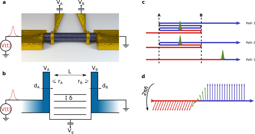
Figure 1: Schematic of the Fabry-Perot cavity and of the main physical mechanism. (a,b) Schematic of our setup, a quantum wire connected to two electrodes. Two barriers A and B separated by a distance $L$ are placed along the wire and a Gaussian voltage pulse $V(t)$ is sent from the left. The barriers are characterized by the barrier heights ($V_{A}$ and $V_{B}$) or equivalently by their reflection and transmission amplitudes denoted respectively $r_{A},r_{B}$ and $d_{A},d_{B}$. A gate voltage $V_{g}$ allows one to shift the position of the resonant levels of the cavity. The mean level spacing between the discrete levels of the cavity is $\delta=h/(2\tau_{F})$ where $\tau_{F}$ is the ballistic time of flight from A to B. (c) Schematic of the physical mechanism for the dynamical control of the interference: as the pulse propagates along the different trajectories, a phase difference $2\pi\bar{n}$ appears between the front (blue) and the rear (red) resulting in a modification of the interference pattern. (d) Graphical representation of Eq. (5) that gives the structure of a voltage pulse in terms of a “phase domain wall”.

Results
Fabry-Perot cavity. Fig. 1a and 1b show our model Fabry-Perot system: it consists of a quantum wire connected to two metallic electrodes. The quantum wire is made into a Fabry-Perot interferometer by means of two barriers (A and B) which can be defects in the wire, gates (as in the sketch) or simply the Schottky barriers that naturally form at the wire-electrode interfaces. Such Fabry-Perot interferometers are standard devices of nanoelectronics and their DC properties have been extensively measured FabryPerot_pioneer ; FabryPerot_carbon_nano ; InAsFP . The basic properties of this interferometer can be understood within an elementary theory. Each barrier A (and B) is described by the amplitude of probability $d_{A}$ ($r_{A}$) for an incident electron to be transmitted (reflected). Summing up the probability amplitudes for all the trajectories (direct transmission: $d_{B}d_{A}$, one back and forth bouncing: $d_{B}r_{A}r_{B}d_{A}$…), the total amplitude of probability for an electron to be transmitted reads,

$$d_{AB}(E)=\frac{d_{A}d_{B}}{1-r_{A}r_{B}z}.$$ (2)

The factor $z$ corresponds to the phase $z=e^{i2kL}$ accumulated by the electron during the time between two collisions ($L$ distance between the scatterers, $k$ electron momentum). $z$ can also be rewritten as $z=e^{i2\tau_{F}E/\hbar}$, where $\tau_{F}$ is the time of flight between A and B, and $E$ is the incident energy (our analytical treatment ignores the small energy dependence of $\tau_{F}$, $d_{A}$,$d_{B}$…but our numerics fully accounts for it). When $E$ is at resonance with the eigenenergies $E_{n}=n\delta+eV_{g}$ of the cavity formed by A and B ($\delta=h/(2\tau_{F})$: mean level spacing, $eV_{g}$: potential shift due to a nearby electrostatic gate), $d_{AB}$ shows a sharp peak and reaches perfect transmission.

Let us now apply a voltage pulse $V(t)$ of duration $\tau_{P}$ and maximum intensity $V_{P}$ to the left electrode. Defining the transmitted current $I_{t}(t)$ just after the second barrier, the observable of interest to us will be the total number $n_{t}=\int I_{t}(t)dt/e$ of electrons transmitted through the system. $n_{t}$ can be directly measured experimentally and requires much less effort than e.g. noise measurements. In an actual experiment, one would measure the DC current $I_{dc}$ upon sending periodic trains of pulses through the system. Indeed, by periodically applying the above pulse with a period $\Theta\gg\tau_{P}$, one simply finds $I_{dc}=en_{t}/\Theta$.

The limit of long pulses $\tau_{P}\gg\tau_{F}$ is rather trivial: as $V(t)$ varies very slowly, at each instant the current follows the DC I-V characteristics of the system: $I_{t}(t)=I_{dc}[V(t)]$ (adiabatic limit) which can be obtained from the Landauer formula. In this limit, $V_{P}\ll\delta$ (linear regime) leads to $n_{t}=|d_{AB}(E_{F})|^{2}\bar{n}$ ($E_{F}$: Fermi level), while for large voltages $V_{P}\gg\delta$ (classical limit) the interference pattern is washed out and one obtains $n_{t}=D_{AB}^{cl}\bar{n}$, where the classical (or incoherent) probability $D_{AB}^{cl}$ corresponds to the addition law of the probabilities associated with the different paths Datta ,

$$D_{AB}^{cl}=\frac{D_{A}D_{B}}{1-R_{A}R_{B}}$$ (3)

(capital letters $D$ or $R$ correspond to the probabilities associated with the respective amplitudes so that $D_{A}=|d_{A}|^{2}$). Eq. (3) is essentially identical to Eq. (2) upon replacing amplitudes by probabilities. So far, we have made rather standard predictions which are easily reproduced by our numerical simulations: the blue symbols in Fig. 2 show that $n_{t}$ oscillates with the gate voltage $V_{g}$ (Fig. 2a) and increases monotonously with $V_{P}$ (Fig. 2b). Fig. 2a has been calculated with an intermediate value of $V_{P}\approx 0.5\delta$ so that the contrast of the interference pattern is not very large.

Having established the adiabatic limit, we can now turn to the more interesting limit of short pulses $\tau_{P}\ll\tau_{F}$ for which a proper time-resolved quantum theory is compulsory. Let us make a naive guess: a very short pulse can be viewed as a very localized perturbation that will propagate ballistically through the wire. Monitoring the current after the barriers, one observes a narrow peak when the perturbation has propagated up to the observation point. $2\tau_{F}$ later one observes a second peak corresponding to trajectories with one reflection on each barrier, new peaks (of increasingly smaller amplitudes) arrive sequentially every $2\tau_{F}$. As the perturbations coming from different trajectories do not coincide in time, they cannot interfere and one expects to observe the “classical” addition law $n_{t}=D_{AB}^{cl}\bar{n}$. The argument can also be made in the energy domain: a fast pulse excites electrons to a large spread in energy which results in an effectively random phase $z$ and the interference pattern gets washed out. A rapid glance at the numerics does indeed confirm this picture: Fig. 3b shows the monitored current $I_{t}(t)$ which clearly shows the peaks described above. Perhaps more transparent is the corresponding color map of the local current $I(x,t)$ (Fig. 3a) where the different trajectories with multiple reflections are clearly visible. In contrast, long pulses (not shown) have an essentially featureless current $I_{t}(t)$ of the same shape as the voltage pulse.

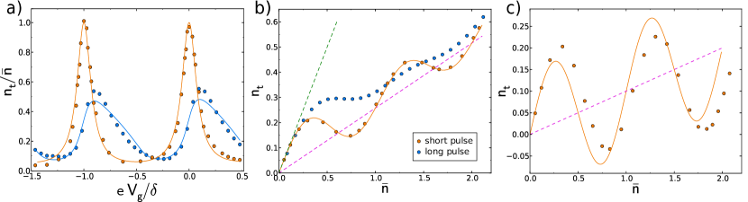
Figure 2: Total charge transmitted $n_{t}$. (a) $n_{t}$ as a function of gate voltage $eV_{g}/\delta$. (b,c) $n_{t}$ as a function of total injected charge $\bar{n}$. The symbols correspond to numerical data for short (blue, $\tau_{P}=\tau_{F}/7$) and long (red, $\tau_{P}=3\tau_{F}$) pulses while the full lines correspond to the analytical results for $\tau_{P}\ll\tau_{F}$ (blue) and $\tau_{P}\gg\tau_{F}$ (red). (a): $V_{P}=0.5\delta$ and $D_{A}=D_{B}=0.5$. (b,c) System at resonance and $V_{P}$ is varied with $D_{A}=D_{B}=0.5$ (b), and $D_{A}=D_{B}=0.1$ (c). Dashed lines: $n_{t}=D_{AB}\bar{n}$ (green) and $n_{t}=D^{Cl}_{AB}\bar{n}$ (magenta).

The story could end here: slow pulses allow one to observe the interference effects (wave aspect of quantum mechanics) while fast pulses give access to the ballistic propagation and reflection/transmission of the charges injected by the pulse (particle aspect of quantum mechanics). A deeper look at the numerics reveals however a handful of rather counter-intuitive physical effects. First, one observes in the $I_{t}(t)$ plot of Fig. 3b that the current does not vanish in between consecutive peaks. Second, Fig. 2 shows that the total number of transmitted electrons in fact oscillates strongly with the gate voltage (Fig. 2a) in total contradiction with the above picture. Indeed, upon using faster pulses, one actually restores the interference pattern that was somewhat smeared in the long pulse case. Third, and even more striking, are Fig. 2b and Fig. 2c which show that the number of transmitted electrons actually oscillates with the number of injected electrons $\bar{n}$. Fig. 2c is particularly intriguing: for $\bar{n}=0.8$, $n_{t}$, e.g. the DC current for a train of pulse, is negative. In other word, one raises the energy of the electrons on the left and the electrons flow toward the left electrode.

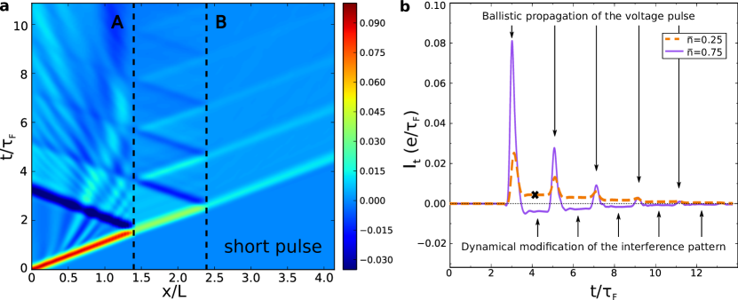
Figure 3: Propagation of the voltage pulse. (a) Local current $I_{t}(x,t)$ as a function of space (in unit of the length $L$ of the cavity) and time (in unit of $\tau_{F}$) for $V_{P}=1.5\delta$, $\tau_{P}=\tau_{F}/3.5$ and the cavity is at resonance. The dashed lines indicate the positions of the barriers. (b) $I_{t}(x_{0},t)$ for $x_{0}=2.5L$ on the right of the second barrier $B$. In orange: $V_{P}=1.5\delta$, in purple: $V_{P}=4.5\delta$ and $\tau_{P}=\tau_{F}/3.5$. The black cross ($\boldsymbol{\times}$) marks the time associated with Fig. 1c.

Dynamical control of the interference pattern. To understand this regime of fast pulses, one needs to develop a proper representation of what a fast voltage pulse really does to the electronic wave function. The naive image where a voltage pulse generates some sort of localized wave packet that propagates through the system is, to a large extent, wrong. In contrast, stationary delocalized waves already exist before the pulse. Ignoring for a moment the presence of the interferometer (barriers), the stationary wave function is a simple plane wave $\Psi(x,t)=e^{ikx-iEt}$. Upon applying a voltage pulse $V(t)\theta(-x)$ (we suppose that the voltage drop is very abrupt spatially for the sake of the argument, $\theta(x)$ is the Heaviside function), the energy of the wave is increased and the wave function starts to accumulate an extra phase $\phi(t)=\int_{-\infty}^{t}du\ eV(u)/\hbar$ for $x<0$. Noting that $\lim_{t\rightarrow\infty}\phi(t)=2\pi\bar{n}$, one finds that the wave function after the pulse takes the form

$$\Psi(x,t)=e^{-i2\pi\bar{n}+ikx-iEt/\hbar}\ \ {\rm for}\ \ x<0$$

$$\Psi(x,t)=e^{+ikx-iEt/\hbar}\ \ {\rm for}\ \ x>0.$$ (4)

The effect of a voltage pulse is therefore to generate a kink in the phase of the electronic wave function $\Psi(x,t)$ (see Fig. 1d for a schematic). In other words, what propagates is essentially a “phase” domain wall between two regions which are characterized by an $e^{i2\pi\bar{n}}$ phase difference. Phases in quantum mechanics cannot be observed directly and one has to resort to interferences between different paths to observe them. The role of the electronic interferometers used in this study is to introduce these different paths. While the argument above is very naive, it correctly captures the main feature of the wave function which reads (for a linearized spectrum),

$$\Psi(x,t)=e^{-i\phi(t-x/v)+ikx-iEt/\hbar}$$ (5)

where $v=(1/\hbar)\partial E/\partial k$ is the group velocity.

Let us now return to our Fabry-Perot cavity. In this case, the stationary wave is not a simple plane wave but a superposition of several waves corresponding to the different paths that the electrons can take (with zero, one, two… reflections) as shown in Fig. 1c. When a voltage pulse is sent through this superposition of paths, it propagates through the various paths. Fig. 1c corresponds to a snapshot at a particular time where the pulse has emerged from the direct path (path 1 of stationary amplitude $d_{B}d_{A}$) but not yet from the longer trajectories with multiple reflections (path 2 of amplitude $d_{B}(r_{A}r_{B})d_{A}$, path 3 of amplitude $d_{B}(r_{A}r_{B})^{2}d_{A}$…). The time at which this snapshot is taken corresponds to the cross in the $I_{t}(t)$ plot of Fig. 3b. If one looks at the wave function just after the barrier B at that particular time, one finds that the amplitude of path 1 has an extra phase $e^{i2\pi\bar{n}}$ compared with its stationary value (rear of the pulse as compared with paths 2, 3,… that are still in the front of the pulse). Therefore at this particular time, the total amplitude is $e^{i2\pi\bar{n}}d_{B}d_{A}+d_{B}(r_{A}r_{B})d_{A}+d_{B}(r_{A}r_{B})^{2}d_{A}$…and is dynamically modified with respect to its stationary value. As time increases, the pulse will emerge from path 2, path 3…and the factor $e^{i2\pi\bar{n}}$ will progressively spreads to all trajectories until one recovers the stationary amplitude (up to a now irrelevant global $e^{i2\pi\bar{n}}$ phase factor). The above argument explains the origin of the plateaus observed in Fig. 3b. The value of the current at these plateaus obviously oscillates with $2\pi\bar{n}$ which consequently explains the oscillations of $n_{t}$. This mechanism, to which we refer to as the dynamical control of the interference pattern, is the main new concept of this paper.

In order to make the above argument quantitative, and in particular properly take into account the Fermi statistics for the filling of the stationary states, we perform the analytical calculation of $n_{t}$ with a “photo-assisted tunneling” formula (Eq. (95) of ref. Twave_formalism, ),

$$n_{t}= \int\frac{dE}{2\pi}\frac{dE^{\prime}}{2\pi}|d_{v}(E^{\prime}-E)d_{AB}(E^{\prime})|^{2}[f(E)-f(E^{\prime})]$$ (6)

where $d_{v}(E^{\prime}-E)$ is the amplitude of probability for an electron with energy $E$ to be transferred to the energy $E^{\prime}$ by the pulse and $f(E)$ the Fermi function. $d_{v}(E^{\prime}-E)$ is essentially the Fourier transform of the phase $e^{-i\phi(t)}$. The calculation of $n_{t}$ for fast pulses yields (see the Methods section),

$$n_{t} =D_{AB}^{cl}\ \bar{n}+[D_{AB}(V_{g})-D_{AB}^{cl}]\frac{\sin(2\pi\bar{n})}{2\pi}$$

$$-\frac{2D_{AB}(V_{g})D_{AB}^{cl}r_{A}r_{B}}{\pi D_{A}D_{B}}\sin^{2}(\pi\bar{n})\sin(2\pi V_{g}/\delta).$$ (7)

Equation (Dynamical control of interference using voltage pulses in the quantum regime) contains two contributions of different kind: the first term, “particle” like, accounts for the ballistic propagation of the pulse while the second and third terms, “wave” like, corresponds to the dynamical modification of the interference pattern discussed above which originates from the difference of phase between the front and the back of the pulse. This interference effect dominates for a resonant Fabry-Perot in the tunneling regime ($D_{A},D_{B}\ll 1$) where the “particle” term vanishes and one observes a purely oscillating signal $n_{t}=[\sin(2\pi\bar{n})]/(2\pi)$, see the right panel of Fig. 2. In particular for $\bar{n}=3/4$, one finds a negative transmitted charge $n_{t}=-1/(2\pi)$ which is a pure interference effect: the $e^{i3\pi/2}$ phase of the pulse dynamically brings the Fabry-Perot cavity out of resonance and as a result, the particles coming from the left are temporarily blocked. The electrons coming from the right, on the contrary, are not affected by the pulse. Therefore the current compensation between left and right is temporarily withstood and one observes a negative net current (see the purple line in Fig. 3b for instance).

Discussion
The requirements to observe the above predictions experimentally are threefold. (i) One needs a device where Fabry-Perot interferences can be observed at DC which implies that the temperature $k_{B}T$ is smaller than the mean level spacing $\delta=h/2\tau_{F}$ of the cavity. (ii) One needs values of $\tau_{F}$ long enough compared with the speed of available pulse generators. (iii) An important ingredient of the modeling is that the voltage drop needs to be spatially abrupt (with respect to the distance $L$ between the two barriers A and B). The spatial shape of the voltage drop is controlled by the ratio between the electric $C$ and quantum $e^{2}\rho$ capacitances of the system, as discussed in section 8.4 of ref. Twave_formalism . In order to obtain a large ratio $C/(e^{2}\rho)$ one needs a very small density of state $\rho$ and/or to use nearby metallic gates in order to obtain an efficient screening of the charges inside the device. Requirement (iii) requires some care but various strategies can be used to enforce it, such as depositing screening gates close to the electron gas or using systems with extremely low density of states. One needs $\delta\geq 10k_{B}T$ in order to fulfill (i) with a good contrast which translates into $\tau_{F}\leq 250ps$ for a typical dilution fridge temperature of $10mK$. This in turn imposes a pulse duration $\tau_{P}\approx 100ps$ to enter the regime of fast pulses. Such requirements are stringent but definitely within grasp of current technology.

There are many possible systems where the above physics could be measured. Recent progress on Thz detection were made with carbon nanotubesMcEuen2008 , for instance, although these objects are rather small (which implies small time of flight hence the THz physics). In the rest of this article, we explore an implementation, perhaps the simplest one, where the interferometer is constructed out of the edge states of a two dimensional electron gas in the quantum Hall regimeFabryPerot_pioneer . The one dimensional edge states have very low density of states and can be further screened by nearby metallic gates or other nearby edge states (at filling factor two). With drift velocities $v_{D}\approx 10^{4}-10^{5}m.s^{-1}$ and a phase coherence length20mum_20mK $L_{\phi}\approx 20\mu m$ at 20mK, one finds that a rather large system of length of a few $\mu m$ should meet the requirements.

We simulated an electronic analogue of a Mach-Zehnder interferometer as sketched in the inset of Fig. 4. The device is close to the ones measured experimentally e.g. in ref. 20mum_20mK (although smaller due to computational limitations) and simulated in DC in ref. Knit . It consists of a two dimensional gas under magnetic field with three terminals and two quantum point contacts which serve as beam splitters. This device differs from the Fabry-Perot in two ways: first it is simpler conceptually as only two paths contribute to the transport. Second, these two paths can be resolved spatially (the edge states being chiral, transmitted and reflected waves propagate on different edge states).

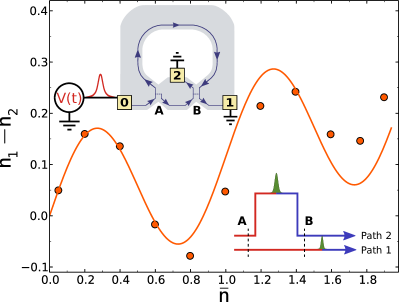
Figure 4: Voltage pulse in a Mach-Zehnder interferometer in the quantum Hall regime. Main figure: difference $n_{1}-n_{2}$ between the transmitted charge into contact one and two as a function of the total injected charge $\bar{n}$. The full line corresponds to the analytical calculation $n_{1}-n_{2}=0.12\bar{n}+0.14\sin(2\pi\bar{n})$ (see Methods section). Upper inset: schematic of the system with the electron gas (light gray), the three contacts 0, 1, and 2 (yellow), the two semi-transparent quantum point contact A and B and the effective chiral edge states (blue arrows). Lower inset: schematic of the two paths which contribute to the stationary wave function. As the pulse propagates along the different trajectories, a phase difference $2\pi\bar{n}$ appears between the front (blue) and the rear (red) of the pulse.

Fig. 4 shows the result of the simulation for a $2\mu m^{2}$ sample with a density of $n_{s}=10^{11}cm^{-2}$, mobility $\mu=2\times 10^{6}cm^{2}.V^{-1}.s^{-1}$ under a magnetic field $B=1.8T$. The velocity is measured to be $v=7\times 10^{4}m.s^{-1}$ with an abrupt confinement of the electrons so that the difference of time of flight between the two paths is $\tau_{F}=64ps$. Fast pulses of duration $\tau_{P}=12ps$ were applied to electrode 0 to obtain the fast pulse limit. The system was discretized on a $3nm$ mesh so that around $10^{5}$ sites were used in the simulation. The results of Fig. 4 confirm the oscillations of the transmitted charge with $\bar{n}$: the dynamical control of the phase between the two arms of the interferometer stands in this experimentally accessible geometry.

Fig. 5c shows the current arriving in the electrode 1 as a function of time, in direct analogy with Fig. 3b: the two peaks correspond respectively to the arrival of the pulse from the lower arm and upper arm of the interferometer while the plateau in between corresponds to the dynamical control of the interference pattern. We show for completeness the actual value of these currents at the first peak ($t=t_{a}$) and on the plateau ($t=t_{b}$) in Fig. 5a and Fig. 5b respectively. We find, as expected, that the first contribution increases with $\bar{n}$ while the latter oscillates as $\sin(2\pi\bar{n})$. The lower inset of Fig. 4 contains a schematic of a snapshot of the interference pattern at $t=t_{b}$.

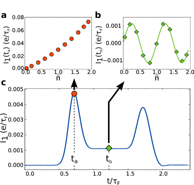
Figure 5: Current $I_{1}$ at contact $1$ for the Mach-Zehnder interferometer (a) and (b) Amplitude of $I_{1}(t_{a})$, $I_{1}(t_{b})$, as a function of the number of injected particles $\bar{n}$. Symbols are numerical data. The line in (b) corresponds to $I_{1}(t_{b})=0.001\sin(2\pi\bar{n})$. (c) Transmitted current $I_{1}(t)$ as a function of time for $\bar{n}=0.2$.

Experiments have now reached the technological threshold where they can be made fast and cold enough for the physics of this proposal to be accessible in the labGlattli . As the available measuring apparatus are getting faster every day, many other nanoelectronics systems will reveal intriguing new physical effects when probed with very fast pulses. In particular, the concept of dynamical control of the interference pattern developed here is very generic and could be extended beyond the physics of electronic interferometers. For instance, Andreev resonant states which form on the boundary of superconductors or the oscillatory magnetic exchange interaction in magnetic multilayers are closely related to the Fabry-Perot physics discussed here, and could be addressed in a similar way. The capability to simulate such time-resolved quantum nanoelectronic circuits, demonstrated here, should play a key role in proposing and analyzing these upcoming experiments.

Methods
Model for the Fabry-Perot geometry. We model the Fabry-Perot cavity with a one dimensional Hamiltonian

$$\mathrm{\hat{\textbf{H}}}(t) =\int dx-\frac{\hbar^{2}}{2m}\psi^{\dagger}(x)\Delta\psi(x)$$

$$+\epsilon(x)\psi^{\dagger}(x)\psi(x)+\theta(-x)eV(t)\psi^{\dagger}(x)\psi(x)$$ (8)

where the field operator $\psi(x)$ [$\psi^{\dagger}(x)$] destroys (creates) an electron at position $x$, $V(t)$ is the voltage pulse applied on the left electrode ($x<0$) and $\epsilon(x)$ the static potential that defines the Fabry-Perot (for $x>0$). We discretize the model on a lattice with lattice distance $a$ and get,

$$\mathrm{\hat{\textbf{H}}}(t)= 2\gamma+\sum_{i=1}^{N+1}\epsilon_{i}c^{\dagger}_{i}c_{i}-\gamma\sum_{i=-\infty}^{+\infty}c^{\dagger}_{i+1}c_{i}$$

$$-\gamma[e^{i\phi(t)}-1]c^{\dagger}_{1}c_{0}+h.c.$$ (9)

where $\gamma=\hbar^{2}/(2ma^{2})$ and $\phi(t)=\int_{-\infty}^{t}dt^{\prime}\ eV(t^{\prime})/\hbar$ (a standard gauge transformation has been applied to transform the time dependent potential for $i\leq 0$ into a time dependent hopping between sites $0$ and $1$). The operator $c_{i}$ ($c^{\dagger}_{i}$) destroys (creates) an electron on site $i$. $\epsilon_{i}$ defines the Fabry-Perot cavity of size $L=Na$: $\epsilon_{1}=V_{A}$, $\epsilon_{N+1}=V_{B}$ and $\epsilon_{i}=-V_{0}+V_{g}$ in the central region $i=\in\{2,3,\dots N\}$. We use Gaussian voltage pulses of width $\tau_{P}$ and maximum voltage $V_{P}$,

$$V(t)=V_{P}\exp\left(-4\log(2)\frac{t^{2}}{\tau_{P}^{2}}\right)$$ (10)

for which $\bar{n}=\kappa eV_{P}\tau_{P}/\hbar$ where $\kappa=1/4\sqrt{\pi\log(2)}\approx 0.17$. Note that contrary to the noise propertiesLevitov1996 ; Lorentzian_pulses ; Ivanov , the total number of transmitted electrons is to a wide extent insensitive to the precise shape of the pulse.

Numerical method. The DC numerical simulations were performed with the Kwant software packagekwant . The time-dependent simulations were performed using the WF-D method of ref. Twave_formalism, which is summarized below. The method consists of three steps. First, we start by solving the stationary problem for times before the pulse. We obtain the two scattering states $\Psi_{\alpha E}^{st}(i)$ of the system for electrons coming from the left $\alpha=L$ and from the right $\alpha=R$ for incident energy $E$. Solving the scattering states of a time independent Hamiltonian is a well studied problem for which efficient techniques have been developedWimmer_thesis . Second, once the pulse starts (say at $t_{0}<0$), we simply integrate the time dependent Schrodinger equation with $\Psi_{\alpha E}(i,t_{0})=\Psi_{\alpha E}^{st}(i)$. More specifically, we introduce the deviation ${\bar{\Psi}}(i,t)$ from the stationary wave function $\Psi_{\alpha E}(i,t)={\bar{\Psi}}(i,t)+e^{-iEt}\Psi_{\alpha E}^{st}(i)$, which satisfies ${\bar{\Psi}}(i,t_{0})=0$. The finite system of $N$ sites is then embedded into a larger finite system of $2M$ sites (with typically $M=1.5N$) and ${\bar{\Psi}}(t)$ satisfies,

$$i\partial_{t}\bar{\Psi}(i,t)=-\gamma[\bar{\Psi}(i+1,t)+\bar{\Psi}(i-1,t)]+(2\gamma+\epsilon_{i})\bar{\Psi}(i,t)$$

$$-\gamma\delta_{i,0}[e^{i\phi(t)}-1][e^{-iEt}\Psi_{\alpha E}^{st}(1)+\bar{\Psi}(1,t)]$$

$$-\gamma\delta_{i,1}[e^{-i\phi(t)}-1][e^{-iEt}\Psi_{\alpha E}^{st}(0)+\bar{\Psi}(0,t)]$$

$$+(\delta_{i,-M}+\delta_{i,+M})\Sigma(E)\bar{\Psi}(i,t)$$ (11)

where the non-Hermitian term $\Sigma(E)=(E-2\gamma)/2\gamma^{2}-i\sqrt{E/\gamma^{3}-E^{2}/4\gamma^{4}}$ is the so-called self-energy of the wire. The integration of Eq. (Dynamical control of interference using voltage pulses in the quantum regime) for different energies is done in parallel on different processors using a 3^rd order Adams-Bashforth scheme. In the last step, the results are integrated over the different energies to obtain the observables. In particular the current at site $i$ reads,

$$I(i,t)=2\frac{e\gamma}{\hbar}{\rm Im}\sum_{\alpha}\int\frac{dE}{2\pi}f(E)\Psi_{\alpha E}^{*}(i,t)\Psi_{\alpha E}(i+1,t)$$ (12)

where $f(E)$ is the Fermi function at temperature $T$ for the Fermi energy $E_{F}$. This method allows one to study systems with $10^{4}-10^{5}$ sites on a simple cluster and is expected to scale beyond $10^{6}$ sites on a supercomputer.

Parameter set for the Fabry-Perot geometry. Most of the data presented here were obtained with the following set of parameters: $N=70$ and $E_{F}=\gamma$ so that $\tau_{F}\approx 35\gamma^{-1}$ and $\delta\approx 0.09\gamma$. Various durations of the pulses were used from $\tau_{P}=5\gamma^{-1}$ to $\tau_{P}=100\gamma^{-1}$. We found that $\tau_{P}\geq 5\gamma^{-1}$ is necessary to enforce $\hbar/\tau_{P}\ll E_{F}$ and get rid of spurious effects associated with the band width of the model. The values of $V_{A}$ and $V_{B}$ are given in Fig. 6b while $V_{0}=-1.068$.

A comment on electron-electron interactions. A common difficulty encountered in time dependent transport, which was pointed out by Buttiker some years agoButtiker_dynamic_conductance , is the crucial role of electrostatics in restoring a gauge invariant, current-conserving theory. Indeed, in the non-interacting theory used here, the conservation equation for the charge reads,

$$\partial_{t}\rho(x,t)+\partial_{x}I(x,t)=0$$ (13)

where $\rho(x,t)$ is the charge density and $I(x,t)$ the local current. In presence of time dependent perturbations (such as the voltage pulse), the current is not conserved and a finite charge density temporary accumulates in the system. An accumulation of charge costs however a tremendous amount of electrostatic energy so that in real systems, this charge density is screened by image charges in nearby gates. Those image charges result in a displacement current $I_{d}=\partial_{t}\rho(x,t)$ flowing in those electrodes. Only once this displacement current is taken into account does one recover current conservation. As a result of the presence of this time dependent charge density, one should, at the mean field level include the corresponding time dependent potential created by these charges into our time dependent Schrodinger equation. Let us make four specific remarks for the situation studied in this article. First, we study situations with a small number of injected particles $\bar{n}$, therefore one should be very careful with the mean field approach as one wants to avoid spurious self interacting terms present at the Hartree level. Second, all our calculations are done for a non-interacting model, and are therefore a priori expected to be valid in presence of metallic gates in close proximity to the quantum wire. Third, while the displacement currents and corresponding time dependent potentials can modify the a.c. properties of the system, the total transmitted charge $n_{t}$ shall not be affected by treating explicitly the electrostatic problem. Indeed, the total number of transmitted and reflected electrons form conserved and gauge invariant quantities (in the sense defined by ButtikerButtiker_dynamic_conductance ) and therefore do not suffer from the flaws of their a.c. counterparts. In plainer words, the integral (over time) of the displacement currents as well as the corresponding time dependent potentials is zero, therefore their presence do not modify $n_{t}$. Finally, recent experimentsGlattli with fast voltage pulses indicate that the non-interacting theory works remarkably well for those systems. A longer discussion of current conservation and gauge invariance can be found in ref. Twave_formalism, .

Note that beside the above mentioned aspects, the electrostatics remains crucial in the determination of the spatial profile of the voltage drop created by the voltage pulse. In order to observe the effects discussed in this article, one needs to be able to create spatially localized voltage drops that can subsequently propagate inside the interferometer. The corresponding condition has been discussed in section 8.4 of ref. Twave_formalism, which we refer to.

Calibration of the Fabry-Perot geometry. Fig. 6 shows the DC characteristics which were used to calibrate our device. Fig. 6a and Fig. 6b show the transmission probability of a single barrier, say A, as a function of the Fermi energy (a) and $V_{A}$. Fig. 6c shows the transmission probability (conductance in unit of $e^{2}/h$) of the full Fabry-Perot cavity as a function of the gate voltage $V_{g}$ from which we can extract the peak to peak mean level spacing $\delta=0.09\gamma$.

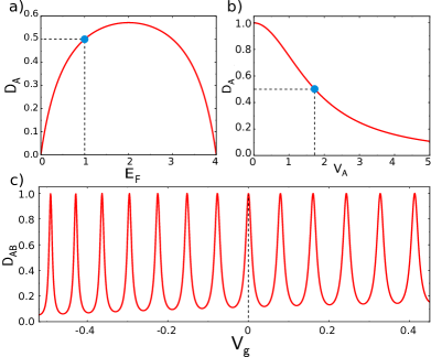
Figure 6: DC characterization of the Fabry-Perot cavity. (a) Transmission of the barrier A as a function of energy $E_{F}$ with $V_{A}=1.73\gamma$. (b) Transmission of barrier A as a function of $V_{A}$ for $E_{F}=1\gamma$. (c) Transmission probability $D_{AB}$ of the entire system with two barriers as a function of $V_{g}$ for $V_{A}=V_{B}=1.73\gamma$ and $E_{F}=1\gamma$ ($D_{A}=D_{B}=0.5$). The parameters of panel (c) correspond to the blue circles of panel (a) and (b).

Fig. 7a shows the resonant and off resonance signal $n_{t}/\bar{n}$ as a function of the maximum voltage $V_{P}/\delta$ for both the short and long pulses. As the visibility of the fast pulses is sensitive to $\bar{n}$ and not to $V_{P}/\delta$ [Eq. (Dynamical control of interference using voltage pulses in the quantum regime)], we find that the system can retain a high visibility for $V_{P}>\delta$ while the interference pattern of the long pulse is totally smeared out. We study in Fig. 7b the temperature dependence of $n_{t}$ at and off resonance. We find that a low $k_{B}T\leq 0.1\delta$ temperature is needed to observe interferences with a good visibility. This requirement is as stringent as the DC requirement but not more, so that temperature should not be a restriction for the observation of the effects predicted in this work.

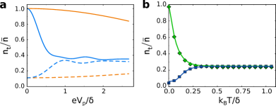
Figure 7: Effect of voltage amplitude and temperature on the visibility of the interference pattern. (a) Transmission probability $n_{t}/\bar{n}$ as a function of $V_{P}/\delta$ for a system at resonance (full lines, $V_{g}=0$) and off resonance (dashed line, $V_{g}=\delta/2$) for a short (orange, $\tau_{P}=\tau_{F}/7$) and long (blue, $\tau_{P}=3\tau_{F}$) pulse. $D_{A}=D_{B}=0.5$. (b) Transmission probability $n_{t}/\bar{n}$ as a function of temperature for the same short pulse and $V_{P}=0.5\delta$. Symbols: numerical results, lines: energy average $\langle-D_{AB}(V_{g},E)\partial_{E}f(E)\rangle_{E}$. The upper curves correspond to $V_{g}=0$ (resonance) while the lower one is off resonance $V_{g}=\delta/2$.

Last, Fig. 8 presents the number of transmitted electrons as a function of the injected one for two different pulse shapes: a Gaussian pulse [Eq. (10)] and a Lorentzian one ($V(t)=V_{P}/(1+4t^{2}/\tau_{P}^{2})$). We find, as expected from the analytical calculation, that the results are insensitive to the shape of the pulse in the fast pulse limit and we recover the oscillating behavior with respect to $\bar{n}$. We emphasize that this is in sharp contrast with the current noise in the single barrier case studied in ref. Lorentzian_pulses,

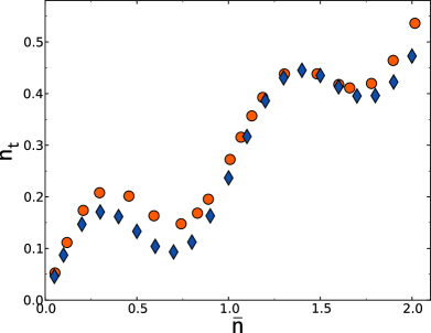
Figure 8: Effect of the shape of the pulse. Transmitted charge $n_{t}$ as a function of total injected charge $\bar{n}$. The system is at resonance and $V_{P}$ is varied with $D_{A}=D_{B}=0.5$. Orange circles are the data of the short Gaussian pulse case from Fig. 2b, blue diamonds correspond to a Lorentzian shaped pulse with width $\tau_{P}=\tau_{F}/7$.

Analytical technique for the calculation of $n_{t}$. Our starting point for the calculation of $n_{t}$ is Eq. (95) of ref. Twave_formalism, ,

$$n_{t}= \int\frac{dE}{2\pi}\frac{dE^{\prime}}{2\pi}|d(E^{\prime},E)|^{2}[f(E)-f(E^{\prime})]$$ (14)

where $d(E^{\prime},E)$ is the amplitude of probability for an incident electron coming from the left with energy E to be transmitted with energy $E^{\prime}$. $d(E^{\prime},E)$ can be further decomposed into

$$d(E^{\prime},E)=d_{v}(E^{\prime}-E)d_{AB}(E^{\prime})$$ (15)

where the first (inelastic) term originates from the voltage drop while the second comes from the (elastic) Fabry-Perot cavity. In order to derive Eq. (14), we have made use of the fact that the transmission amplitude $d_{v}^{\prime}(E^{\prime}-E)$ for electrons coming from the right is given by $d_{v}^{\prime}(E^{\prime}-E)=d_{v}^{*}(E-E^{\prime})$. Note that Eq. (14) as a whole is a perfectly convergent integral whose integrand is concentrated around the Fermi level (assuming the voltage pulse is slow enough compared with $\hbar/E_{F}$). However each of its two sub terms spread over the entire band of the model, so one should refrain from calculating these two terms separately, if possible. Eq. (14) has a nice straightforward interpretation: one simply sums over the (incoherent) incoming states and calculate their total transmission probabilities regardless of the final energy. In the absence of voltage pulse the vanishing $n_{t}$ comes from the compensation between electrons coming from the left and from the right.

Our model for the Fabry-Perot transmission amplitude has been given in the core of the text. To calculate $d_{v}(E^{\prime}-E)$, one defines the scattering states on both sides of the voltage drop:

$$\Psi_{L}(n,t) =\frac{1}{\sqrt{v(E)}}e^{ik(E)n-iEt}$$ (16)

$$+\int\frac{dE^{\prime}}{2\pi}r_{v}(E^{\prime},E)\frac{1}{\sqrt{v(E^{\prime})}}e^{-ik(E^{\prime})n-iE^{\prime}t}$$

on the left and

$$\Psi_{R}(n,t)=\int\frac{dE^{\prime}}{2\pi}d_{v}(E^{\prime},E)\frac{1}{\sqrt{v(E^{\prime})}}e^{ik(E^{\prime})n-iE^{\prime}t}$$ (17)

on the right (with $v(E)=\partial E/\partial k$ the velocity associated with the dispersion relation $E=2\gamma\cos k$). By “matching” the left and right waves across the voltage drop (see ref. Twave_formalism, ), one obtains a set of equations for $d_{v}$ and $r_{v}$. In the limit where the pulse is slow $\tau_{P}\gg\hbar/E_{F}$, and $V_{P}\ll E_{F}/e$ is low compared with the Fermi energy, (the case of interest for our nanodevices), we can linearize the dispersion relation and we simply recover the result of ref. Lorentzian_pulses, ,

$$d_{v}(E^{\prime}-E)=\int dte^{i(E^{\prime}-E)t}e^{-i\phi(t)}$$ (18)

with $r_{v}=0$. To proceed, we expand $d_{AB}(E)$ in terms of the different paths,

$$d_{AB}(E)=\sum_{n=0}^{\infty}d_{A}d_{B}(r_{A}r_{B})^{n}e^{2i\tau_{F}(E+eV_{g})n}$$ (19)

and introducing $\epsilon=E^{\prime}-E$, we get,

$$n_{t}= \int\frac{dE}{2\pi}\frac{d\epsilon}{2\pi}\sum_{n,m}|d_{v}(\epsilon)|^{2}D_{A}D_{B}(r_{A}r_{B})^{n+m}$$

$$\times e^{2i\tau_{F}(E+eV_{g})(n-m)}[f(E-\epsilon)-f(E)]$$ (20)

We can now perform the integration over $E$ (at zero temperature) which binds together the two parts of the integral. The terms $n=m$ and $n\neq m$ need to be considered separately, and we get,

$$n_{t} =D_{AB}^{cl}\int\frac{d\epsilon}{2\pi}\ |d_{v}(\epsilon)|^{2}\epsilon+\int\frac{d\epsilon}{2\pi}\ |d_{v}(\epsilon)|^{2}\frac{D_{A}D_{B}}{2\pi}$$

$$\times\sum_{n\neq m}(r_{A}r_{B})^{n+m}\frac{e^{i\alpha_{g}(n-m)}}{i2\tau_{F}(n-m)}(e^{i2\tau_{F}\epsilon(n-m)}-1)$$ (21)

with $\alpha_{g}=2\tau_{F}(E_{F}+eV_{g})/\hbar$. We can now replace $d_{v}(\epsilon)$ by its expression Eq. (18) and performing the integral over $\epsilon$, we arrive at

$$n_{t}=D_{AB}^{cl}\bar{n}+ \sum_{n}\sum_{m\neq n}\frac{D_{A}D_{B}}{2\pi}(r_{A}r_{B})^{n+m}\frac{e^{i\alpha_{g}(n-m)}}{i2\tau_{F}(n-m)}$$ (22)

$$\times\int dt\ \left[e^{-i\phi(t)}e^{i\phi(t+2\tau_{F}(n-m))}-1\right]$$

Eq. (22) applies for all pulses, short and long. Assuming an infinitely short pulse $\phi(t)=\theta(t)e^{i2\pi\bar{n}}$, we obtain after integration and resummation of the geometric series,

$$n_{t}\big{|}_{short} =D_{AB}^{cl}\ \bar{n}+(D_{AB}(V_{g})-D_{AB}^{cl})\frac{\sin(2\pi\bar{n})}{2\pi}$$

$$-\frac{2D_{AB}(V_{g})D_{AB}^{cl}r_{A}r_{B}}{\pi D_{A}D_{B}}\sin^{2}(\pi\bar{n})\sin(2\pi V_{g}/\delta)$$ (23)

In the case of very long pulses $\phi(t)$ evolves very slowly with respect to $\tau_{F}$ so that one expands $\phi(t+a\tau_{F})\approx\phi(t)+a\tau_{F}eV(t)/\hbar$. In this limit, Eq. (22) allows one to recover the adiabatic result,

$$n_{t}\big{|}_{long}=\int dt\int_{E_{F}}^{E_{F}+V(t)}\frac{dE}{2\pi}D_{AB}(E)$$ (24)

The calculation for the Mach-Zehnder geometry proceeds along the same lines, and is even simplified by the presence of only two paths contributing to the transmission amplitude of the device. The transmission probabilities from lead $0$ to $1$ ($2$) reads,

$$|S^{0}_{10}(E)|^{2} =D_{A}D_{B}+R_{A}R_{B}$$ (25)

$$+2\sqrt{D_{A}D_{B}R_{A}R_{B}}\cos(\phi+\tau_{F}(E-E_{F})),$$

$$|S^{0}_{20}(E)|^{2} =D_{A}R_{B}+R_{A}D_{B}$$ (26)

$$-2\sqrt{D_{A}D_{B}R_{A}R_{B}}\cos(\phi+\tau_{F}(E-E_{F})),$$

with $\phi$ the total magnetic flux through the central depleted region (in unit of $\hbar/e$) and $\tau_{F}$ the extra time needed for the upper paths with respect to the lower one. After following the same steps as for the Fabry-Perot geometry, one obtains (in the limit of short pulses) the number of particles transmitted to contact $1$ ($2$),

$$n_{1} =(D_{A}D_{B}+R_{A}R_{B})\bar{n}$$ (27)

$$+\frac{2}{\pi}\sqrt{D_{A}D_{B}R_{A}R_{B}}\sin(\pi\bar{n})\cos(\pi\bar{n}+\phi)$$

$$n_{2} =(D_{A}R_{B}+R_{A}D_{B})\bar{n}$$ (28)

$$-\frac{2}{\pi}\sqrt{D_{A}D_{B}R_{A}R_{B}}\sin(\pi\bar{n})\cos(\pi\bar{n}+\phi)$$

Model for the Mach-Zehnder geometry.

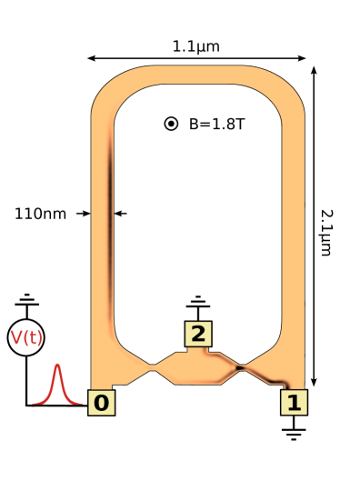
Figure 9: Mach-Zehnder interferometer. Snapshot of the local electronic density at $t=46ps$. The color map indicates the deviation from equilibrium which goes from 0 (salmon) to $0.22\times 10^{11}cm^{-2}$ (black).

We consider a two-dimensional electron gas made from a two-dimensional GaAs/AlGaAs heterostructure with high mobility $\mu=2\times 10^{6}cm^{2}.V^{-1}.s^{-1}$, an electronic density $n_{s}=10^{11}cm^{-2}$ and a perpendicular magnetic field $B=1.8T$ (corresponding to filling factor one, first Hall plateau). The three terminal electronic Mach-Zehnder interferometer is sketched in Fig. 9.

The system is modeled within the effective mass approximation in presence of a small static disorder. The Schrodinger equation is discretized on a mesh with a step $a=3nm$ much smaller than both the Fermi wave length $\lambda_{F}=79nm$ and magnetic length $l_{B}=19nm$ of the system. The magnetic field is accounted through a standard Peierls’ substitution. The model and its DC characterization (with a slightly different geometry) were discussed in ref. Knit, .

In the simulations, contacts $1$ and $2$ are grounded, while a voltage pulse is applied on contact $0$ [same pulse as Eq. (10)]. The injected current follows the edge state and is split into two parts as it reaches the first quantum point contact (QPC). Both QPCs are set to be semi-transparent $D_{A}=D_{B}=0.5$ and consequently act as beam splitters. The two parts of the initial current are recombined at the second QPC. Fig. 9 actually corresponds to a snapshot of the simulation at an intermediate time $t=46ps$: the color code indicates the deviation of the local electronic density with respect to the equilibrium value. At this intermediate time, the pulse has already passed through the first QPC and is split into two parts. The lower (transmitted) part is reaching the electrodes 1 and 2 while the upper (reflected) part is traveling along the longer arm of the interferometer.

References

Acknowledgment
This work was supported by the ERC grant MesoQMC from the European Union. We thank C. Groth, P. Roche, M. Houzet, D.C. Glattli, C. Bauerle, P. Roulleau and D. Luc for very valuable discussions.

Author contributions
X.W. initiated the project. B.G. performed the numerical simulations. X.W. and B.G. performed the analytical calculations, data analysis and wrote the manuscript.

Contact information
Correspondence and requests for materials should be addressed to X.W. (email: xavier.waintal@cea.fr)

References

- (1) A. Bertoni, P. Bordone, R. Brunetti, C. Jacoboni and S. Reggiani, Quantum logic gates on coherent electron transport in quantum wires, Phys. Rev. Lett. 84, 5912–5915 (2000).
- (2) P. Samuelsson, E. V. Sukhorukov, and M. Büttiker, Two-particle aharonov-bohm effect and entanglement in the electronic hanbury brown and twiss setup, Phys. Rev. Lett. 92, 026805 (2004).
- (3) A. V. Lebedev, G. B. Lesovik and G. Blatter, Generating spin-entangled electron pairs in normal conductors using voltage pulses, Phys. Rev. B 72, 245314 (2005).
- (4) C. W. J. Beenakker, M. Titov, and B. Trauzettel. Optimal spin-entangled electron-hole pair pump, Phys. Rev. Lett. 94, 186804 (2005).
- (5) G. Fève, P. Degiovanni, and Th. Jolicoeur, Quantum detection of electronic flying qubits in the integer quantum hall regime, Phys. Rev. B 77, 035308 (2008).
- (6) H. Schomerus and J. P. Robinson, Entanglement between static and flying qubits in an aharonov-bohm double electrometer, New J. Phys 9, 12 (2007).
- (7) Y. Ji, Y. Chung, D. Sprinzak, M. Heiblum, D. Mahalu, and H. Shtrikman, An electronic mach-zehnder interferometer, Nature 442, 415 (2003).
- (8) P. Roulleau, F. Portier, P. Roche, A. Cavanna, G. Faini, U. Gennser, and D. Mailly, Direct measurement of the coherence length of edge states in the integer quantum hall regime, Phys. Rev. Lett. 100, 126802 (2008).
- (9) G. Haack, M. Moskalets, J. Splettstoesser, and M. Büttiker, Coherence of single-electron sources from mach-zehnder interferometry, Phys. Rev. B 84, 081303 (2011).
- (10) M. Yamamoto, S Takada, C. Bäuerle, K. Watanabe, A. D. Wieck, and S. Tarucha, Electrical control of a solid-state flying qubit, Nature Nanotechnology 7, 247–251 (2012).
- (11) G. Fève, A. Mahé, J.-M. Berroir, T. Kontos, B. Plaçais, D. C. Glattli, A. Cavanna, B. Etienne, and Y. Jin, An on-demand coherent single-electron source. Science 316, 1169 (2007).
- (12) G. B. Lesovik and L. S. Levitov, Noise in an ac biased junction: Nonstationary Aharonov-Bohm effect, Phys. Rev. Lett. 72, 538–541 (1994).
- (13) L. S. Levitov, H. Lee, and G. B. Lesovik, Electron counting statistics and coherent states of electric current, Journal of Mathematical Physics 37, 4845 (1996).
- (14) J. Keeling, I. Klich, and L. S. Levitov, Minimal excitation states of electrons in one-dimensional wires, Phys. Rev. Lett. 97, 116403 (2006).
- (15) D. A. Ivanov, H. W. Lee, and L. S. Levitov, Coherent states of alternating current, Phys. Rev. B 56, 6839–6850 (1997).
- (16) J. Gabelli and B. Reulet, Shaping a time-dependent excitation to minimize the shot noise in a tunnel junction, Phys. Rev. B 87, 075403 (2013).
- (17) Z. Zhong, N.M. Gabor, J.E. Sharping, A. Gaetal, and P.L. McEuen, Terahertz time-domain measurement of ballistic electron resonance in a single-walled carbon nanotube, Nature Nanotechnology 3, 201 (2008).
- (18) J. Dubois, T. Jullien, F. Portier, P. Roche, A. Cavanna, Y. Jin, W. Wegscheider, P. Roulleau, and D. C. Glattli, Minimal-excitation states for electron quantum optics using levitons. Nature 502, 659 – 663 (2013).
- (19) B. J. van Wees, L. P. Kouwenhoven, C. J. P. M. Harmans, J. G. Williamson, C. E. Timmering, M. E. I. Broekaart, C. T. Foxon, and J. J. Harris, Observation of zero-dimensional states in a one-dimensional electron interferometer, Phys. Rev. Lett. 62, 2523–2526, (1989).
- (20) W. Liang, M. Bockrath, D. Bozovic, J. H. Hafner, M. Tinkham, and H. Park, Fabry - perot interference in a nanotube electron waveguide, Nature 411, 665–669 (2001).
- (21) A.V. Kretinin, R. Popovitz-Biro, D. Mahalu, and H. Shtrikman. Multimode fabry-perot conductance oscillations in suspended stacking-faults-free inas nanowires, Nano Letters 10, 3439 (2010).
- (22) S. Datta, Electronic Transport in Mesoscopic Systems, Cambridge University Press (1997).
- (23) B. Gaury, J. Weston, M. Santin, M. Houzet, C. Groth, and X. Waintal, Numerical simulations of time-resolved quantum electronics, Physics Reports 534, 1 – 37 (2014).
- (24) K. Kazymyrenko and X. Waintal, Knitting algorithm for calculating green functions in quantum systems, Phys. Rev. B 77,115119 (2008).
- (25) M. Wimmer, Quantum transport in nanostructures: From computational concepts to spintronics in graphene and magnetic tunnel junctions, PhD thesis, Universität Regensburg (2006).
- (26) M. Büttiker, A. Prêtre, and H. Thomas, Dynamic conductance and the scattering matrix of small conductors, Phys. Rev. Lett. 70,4114–4117 (1993).
- (27) C. W. Groth, M. Wimmer, A. R. Akhmerov, and X. Waintal, Kwant: a software package for quantum transport, http://arxiv.org/abs/1309.2926 (2013).