Subclasses of Presburger Arithmetic and the
Weak EXP Hierarchy

Abstract

It is shown that for any fixed $i>0$, the $\Sigma_{i+1}$-fragment of Presburger arithmetic, i.e., its restriction to $i+1$ quantifier alternations beginning with an existential quantifier, is complete for $\mathsf{\Sigma}^{\EXP}_{i}$, the $i$-th level of the weak EXP hierarchy, an analogue to the polynomial-time hierarchy residing between $\NEXP$ and $\EXPSPACE$. This result completes the computational complexity landscape for Presburger arithmetic, a line of research which dates back to the seminal work by Fischer & Rabin in 1974. Moreover, we apply some of the techniques developed in the proof of the lower bound in order to establish bounds on sets of naturals definable in the $\Sigma_{1}$-fragment of Presburger arithmetic: given a $\Sigma_{1}$-formula $\Phi(x)$, it is shown that the set of non-negative solutions is an ultimately periodic set whose period is at most doubly-exponential and that this bound is tight.

1 Introduction

Presburger arithmetic is the first-order theory of the structure ${\langle\mathbb{N},0,1,+,<\rangle}$. This theory was shown to be decidable by Presburger in his seminal paper in 1929 by providing a quantifier-elimination procedure Pre29 . Presburger arithmetic is central to a vast number of different areas in computer science and is often employed as a tool for showing decidability and complexity results.

The central decision problem for Presburger arithmetic is validity, i.e., to decide whether a given sentence is true with respect to the standard interpretation in arithmetic. The two most prominent ways to decide validity are either quantifier-elimination based Coo72 or automata based WB95 ; Kla08 ; DGH12 . Any decision procedure for Presburger arithmetic is inherently tied to the computational complexity of Presburger arithmetic; for that reason the complexity of Presburger arithmetic has extensively been studied in the literature from the 1970’s onwards. In order to fully capture the computational complexity of Presburger arithmetic, Berman even introduced the $\mathsf{STA}$ measure on the complexity of a decision problem, since Presburger arithmetic “may not have precise complexity characterisations in terms of the usual time and tape measures” Ber80 . The class $\mathsf{STA}(s(n),t(n),a(n))$ is the class of all problems of length $n$ that can be decided by an alternating Turing machine in space $s(n)$ and time $t(n)$ using $a(n)$ alternations, where “$\ast$” acts as a wildcard in order to indicate an unbounded availability of a certain resource. Based on the work by Fischer & Rabin FR74 and Ferrante & Rackoff FR75 , Berman established the following result.

Proposition 1 (Berman Ber80 ).

Presburger arithmetic is complete for $\mathsf{STA}(\ast,2^{2^{n^{O(1)}}},n)$.

In terms of the usual time and space measures, this settles Presburger arithmetic between 2-$\NEXP$ and 2-$\EXPSPACE$. Despite these high computational costs, on the positive side when looking at fragments Presburger arithmetic becomes more manageable. There are two dimensions in which we can constraint formulas in order to obtain fragments of Presburger arithmetic: the number of quantifier alternations and the number of variables in each quantifier block. For $i,j\in\mathbb{N}\cup\{\ast\}$, let PA($i$,$j$) denote the set of formulas of the $\Sigma_{i}$-fragment of Presburger arithmetic such that at most $j$ different variables occur in each quantifier block, where “$\ast$” is used as a wildcard for an unbounded number. Hence, Proposition 1 characterises the computational complexity of PA($\ast$,$\ast$) with $n$ being the number of symbols required to write down the formula. Subsequently, PA and PA($i$) abbreviate PA($\ast$,$\ast$) and PA($i$,$\ast$), respectively.

One of the most prominent fragments of Presburger arithmetic is its existential or quantifier-free fragment, which is computationally not more expensive than standard Boolean satisfiability.

Proposition 2 (Scarpellini Sca84 , Borosh & Treybing BT76 ).

For any fixed $j\in\mathbb{N}$, PA($1$,$j$) is in $\P$ Sca84 . PA($1$) is $\NP$-complete BT76 .

Due to its comparably low computational complexity, quantifier-free Presburger arithmetic is the fragment that is most commonly found in application areas which aim at a practical impact. The existential fragment of Presburger arithmetic can even be extended with a full divisibility predicate while retaining decidability Lip78 ; Lip81 .

Another subclass of Presburger arithmetic which has extensively been studied is obtained by allowing for an arbitrary but fixed number of quantifier alternations.

Proposition 3 (Grädel Gra88 , Schöning Scho97 , Reddy & Loveland RL78 ).

For any fixed $i>0$ and $j>2$, PA($i+1$,$j$) is $\mathsf{\Sigma}_{i}^{\P}$-complete Gra88 ; Scho97 . PA($i$) is in $\mathsf{STA}(\ast,2^{n^{O(i)}},i)$ RL78 .

Thus, when fixing the number of quantifier alternations, the complexity of Presburger arithmetic decreases roughly by one exponent, and when additionally fixing the number of variables, we obtain every level of the polynomial-time hierarchy. Notice that there is an obvious gap: a completeness result for Presburger arithmetic with a fixed number of quantifier alternations and an arbitrary number of variables in each quantifier block is missing.

The study of lower bounds for PA($i$) goes back to the work of Fürer F82 , who showed a $\NEXP$ lower bound for some fixed $i>1$. Later, Grädel showed $\NEXP$-hardness and $\EXPSPACE$ membership of PA(2), but tight lower and upper bounds for the whole class of PA($i$) formulas have not yet been established. The purpose of the first part of this paper is to close this gap and establish the following theorem.

Theorem 1.

For any fixed $i>0$, the $\Sigma_{i+1}$-fragment of Presburger arithmetic is $\mathsf{\Sigma}^{\EXP}_{i}$-complete.

Here, $\mathsf{\Sigma}^{\EXP}_{i}$ denotes the $i$-th level of the weak EXP hierarchy Hem89 , an analogue to the polynomial-time hierarchy Sto76 residing between $\NEXP$ and $\EXPSPACE$; a formal definition will be provided in Section 2.4. Equivalently, we obtain that PA($i+1$) is complete for $\mathsf{STA}(\ast,2^{n^{O(i)}},i)$. Determining the precise complexity of the $\Sigma_{i}$-fragment of Presburger arithmetic for a fixed $i$ has been listed as a problem that “deserves to be investigated” by Compton & Henson [CH90, , Prob. 10.14]. However, as pointed out in CH90 , their generic methods for proving lower bounds do not seem to be applicable to this fragment, and our hardness result is based on rather specific properties of, for instance, distributions of prime numbers.

The second part of the paper diverts from the first part and focuses on the $\Sigma_{1}$-fragment of Presburger arithmetic. More specifically, we consider sets of naturals definable by formulas in the $\Sigma_{1}$-fragment of Presburger arithmetic open in one variable. Given a $\Sigma_{1}$-formula $\Phi(x)$, denote by $\llbracket\Phi(x)\rrbracket$ the set of those $a\in\mathbb{N}$ such that replacing $x$ with $a$ in $\Phi(x)$ is valid. It is well-known that $\llbracket\Phi(x)\rrbracket$ is an ultimately periodic set, see e.g. Bes02 . A set $N\subseteq\mathbb{N}$ is ultimately periodic if there exists a threshold $t\in\mathbb{N}$, a base $B\subseteq\{0,\ldots t-1\}$, a period $p\in\mathbb{N}$, and a set of residue classes $R\subseteq\{0,\ldots p-1\}$ such that $N=U(t,p,B,R)$ with

$$U(t,p,B,R) \stackrel{{\scriptstyle\text{def}}}{{=}}B\cup\left\{t+r+kp:r\in R,k\geq 0\right\}.$$

Given a $\Sigma_{1}$-formula $\Phi(x)$, by applying some insights from the first part, we can establish a doubly-exponential upper bound on the period of the ultimately periodic set equivalent to $\llbracket\Phi(x)\rrbracket$ and show that this bound is tight, which is captured by the second main theorem of this paper.

Theorem 2.

There exists a family of $\Sigma_{1}$-formulas of Presburger arithmetic $(\Phi_{n}(x))_{n>0}$ such that each $\Phi_{n}(x)$ is a PA($1$,$O(n)$) formula with $\lvert\Phi_{n}(x)\rvert\in O(n^{2})$ and $\llbracket\Phi_{n}(x)\rrbracket$ is an ultimately periodic set with period $p_{n}\in 2^{2^{\Omega(n)}}$. Moreover for any $\Sigma_{1}$-formula $\Phi(x)$, we have $\llbracket\Phi(x)\rrbracket=U(t,p,B,R)$ such that $t\in 2^{\poly(\lvert\Phi(x)\rvert)}$ and $p\in 2^{2^{\poly(\lvert\Phi(x)\rvert)}}$.

The most interesting part about this theorem is the doubly-exponential lower bound of the period of ultimately periodic sets definable by PA($1$) formulas. Establishing bounds on constants of ultimately periodic sets naturally occurs when analysing the computational complexity of decision problems for infinite-state systems GHOW12 or in formal language theory Huy84 . For instance, analysing such bounds has been crucial in order to obtain optimal complexity results for model-checking problems of a class of one-counter automata in GHOW12 . In more detail, in GHOW12 it has been shown that the set of non-negative weights of paths between two nodes in a weighted graph is ultimately periodic with a period that is at most singly-exponential bounded. A result by Seidl et al. SSMH04 on Parikh images of non-deterministic finite-state automata implicitly states that those ultimately periodic sets are definable in the $\Sigma_{1}$-fragment of Presburger arithmetic. It would thus be desirable to establish a generic upper bound for ultimately periodic sets definable in PA($1$) yielding the same optimal bounds. In this context, Theorem 2 provides a negative result in that it shows that a general bound on ultimately periodic sets definable in PA($1$) cannot yield the optimal bounds required for natural concrete ultimately periodic sets like those considered in GHOW12 .

This paper is structured as follows. In Section 2 we provide most of the formal definitions required in this paper; however the reader is expected to have some level of familiarity with standard notions and concepts from linear algebra, integer programming, first-order logic and computational complexity. Even though we provide a slightly more elaborated account on succinct encodings via Boolean circuits, it will be beneficial to the reader to be familiar with Chapters 8 and 20 in Papadimitriou’s book on computational complexity Pap94 . Section 3 is then going to establish the lower and upper bounds of Theorem 1, and Theorem 2 is shown in Section 4. The paper concludes in Section 5. Subsequent to the bibliography, a proof of a technical characterisation of the weak EXP hierarchy is outlined in the appendix for the sake of completeness.

2 Preliminaries

2.1 General notation

By $\mathbb{Z}$ and $\mathbb{N}$ we denote the set of integers and natural numbers, respectively. We will usually use $a,b,c$ for numbers in $\mathbb{Z}$ and $\mathbb{N}$. Given $a\in\mathbb{N}$, we define $[a]\stackrel{{\scriptstyle\text{def}}}{{=}}\{0,\ldots a-1\}$. Given sets $M,N\subseteq\mathbb{N}$, as is standard $M+N\stackrel{{\scriptstyle\text{def}}}{{=}}\{m+n:m\in M,n\in N\}$ and $M\cdot N\stackrel{{\scriptstyle\text{def}}}{{=}}\{mn:m\in M,n\in N\}$. Moreover, we will use standard notation for integer intervals and, e.g., for $a\leq b\in\mathbb{N}$ denote by $[a,b)$ the set $\{a,\ldots b-1\}$. For vectors $\mathbf{a}=(a_{1},\ldots,a_{n})\in\mathbb{Z}^{n}$, we will denote by $\lVert\mathbf{a}\rVert$ the norm of $\mathbf{a}$, which is the maximum absolute value of all components of $\mathbf{a}$, i.e., $\lVert\mathbf{a}\rVert\stackrel{{\scriptstyle\text{def}}}{{=}}\max\{\lvert a_{i}\rvert\}_{1\leq i\leq n}$. For $m\times n$ integer matrices $A$, $\lVert A\rVert$ denotes the maximum absolute value of all components of $A$. Finally, given a set $M\subseteq\mathbb{Z}^{n}$, we denote by $\lVert M\rVert$ the maximum of the norm of all elements of $M$. All functions in this paper are assumed to map non-negative integers to non-negative integers. Unless stated otherwise, we assume all integers in this paper to be encoded in binary, i.e., the size or length to write down $a\in\mathbb{Z}$ is $O(\log\lvert a\rvert)$.

2.2 Presburger Arithmetic

Usually, $x,y,z$ will denote first-order variables, and $\mathbf{x},\mathbf{y},\mathbf{z}$ vectors or tuples of first-order variables. Let $\mathbf{x}=(x_{1},\ldots,x_{n})$ be an $n$-tuple of first-order variables. In this paper, formulas of Presburger arithmetic are standard first-order formulas over the structure ${\langle\mathbb{N},0,1,+,<\rangle}$ obtained from atomic expressions of the form $p(\mathbf{x})<b$, where $p(\mathbf{x})$ is a linear multivariate polynomial with integer coefficients and absolute term zero, and $b\in\mathbb{Z}$. If the dimension of $\mathbf{x}$ is clear from the context, for brevity we will often omit stating it explicitly. Let $\mathbf{a}=(a_{1},\ldots,a_{n})\in\mathbb{N}^{n}$ and $\Phi(\mathbf{x})$ be open in the first-order variables $\mathbf{x}$, we denote by $\Phi(\mathbf{a}/\mathbf{x})$ the closed formula obtained from replacing every occurrence of $x_{i}$ in $\Phi(\mathbf{x})$ with $a_{i}$. By $\llbracket\Phi(\mathbf{x})\rrbracket$ we denote the set $\{\mathbf{a}\in\mathbb{N}^{n}:\Phi(\mathbf{a}/\mathbf{x})$ is valid$\}$. The size $\lvert\Phi\rvert$ of a formula of Presburger arithmetic is defined as the number of symbols required to write it down, and the norm $\lVert\Phi\rVert$ is the largest absolute value of all constants occurring in $\Phi$.

Remark.

For notational convenience, when stating concrete formulas we will permit ourselves to use atomic formulas $p(\mathbf{x})<q(\mathbf{x})$ for linear polynomials $p(\mathbf{x}),q(\mathbf{x})$. Moreover, all results on the complexity of validity of formulas of Presburger arithmetic carry over if we assume unary encoding of numbers, since binary encoding of numbers can be “simulated” by the introduction of additional first-order variables and repeated multiplication by two, causing only a sub-quadratic blowup in the formula size. In addition, an equality predicate “$=$” can be expressed in terms of $<$ causing a linear blowup, since $x=y\leftrightarrow x<y+1\wedge y<x+1$. Likewise, $x>y$ and $x<y<z$ abbreviate $y<x$ and $x<y\wedge y<z$, respectively.

2.3 Semi-Linear Sets and Systems of Linear Diophantine Inequalities

A central result due to Ginsburg and Spanier states that the sets of natural numbers definable by a formula of Presburger arithmetic open in $n$ variables are the $n$-dimensional semi-linear sets Gin66 , which we just call semi-linear sets if the dimension is clear from the context. A semi-linear set is a finite union of linear sets. The latter are defined in terms of a base vector $\mathbf{b}\in\mathbb{N}^{n}$ and a finite set of period vectors $P=\{\mathbf{p}_{1},\ldots\mathbf{p}_{k}\}\subseteq\mathbb{N}^{n}$, and define the set

$$L(\mathbf{b};P)\stackrel{{\scriptstyle\text{def}}}{{=}}\mathbf{b}+\lambda_{1}\mathbf{p}_{1}+\cdots\lambda_{k}\mathbf{p}_{k},~{}\lambda_{i}\in\mathbb{N},1\leq i\leq k.$$

Let $A$ be an $m\times n$ integer matrix and $\mathbf{c}\in\mathbb{Z}^{m}$. A system of linear Diophantine inequalities is given as $S:A\mathbf{x}\geq\mathbf{c}$. The size $\lvert S\rvert$ of $S$ is the number of symbols required to write down $S$ assuming binary encoding of numbers. The set of positive solutions of $S$ is denoted by $\llbracket S\rrbracket\subseteq\mathbb{N}^{n}$ and is the set of all $n$-tuples such that the inequalities in every row of $S$ hold.

The following proposition is due to Frank & Tardos and establishes a strongly polynomial-time algorithm for the feasibility problem of a system of linear Diophantine inequalities in a fixed dimension, i.e., deciding whether $\llbracket S\rrbracket\neq\emptyset$.

Proposition 4 (Frank & Tardos FT87 ).

Let $S:A\mathbf{x}\geq\mathbf{c}$ be a system of linear Diophantine inequalities such that $A$ is an $m\times n$ matrix. Then feasibility of $S$ can be decided using $n^{2.5n+o(n)}\lvert S\rvert$ arithmetic operations and space polynomial in $\lvert S\rvert$.

When we are interested in representing the set of all solutions of $S$, we will employ the following proposition, which provides bounds on the semi-linear representation of $\llbracket S\rrbracket$ and is a consequence of Corollary 1 in Pot91 .

Proposition 5 (Pottier Pot91 ).

Let $S:A\mathbf{x}\geq\mathbf{c}$ be a system of linear Diophantine inequalities such that $A$ is an $m\times n$ matrix. Then $\llbracket S\rrbracket=\bigcup_{i\in I}L(\mathbf{b}_{i};P_{i})$ such that for all $i\in I$,

$$\lVert\mathbf{b}_{i}\rVert,\lVert P_{i}\rVert\leq(n\lVert A\rVert+\lVert\mathbf{c}\rVert+2)^{m+n}.$$

2.4 Time Hierarchies

Let us recall the definitions of the polynomial-time hierarchy $\PH$ Sto76 and the weak EXP hierarchy EXPH Hem89 in terms of oracle complexity classes. As usual,

$$\P =\bigcup_{k>0}\DTIME(n^{k}) \EXP =\bigcup_{k>0}\DTIME(2^{n^{k}})$$

$$\NP =\bigcup_{k>0}\NTIME(n^{k}) \NEXP =\bigcup_{k>0}\NTIME(2^{n^{k}}).$$

The aforementioned time hierarchies are now defined as

$$\mathsf{\Sigma}_{0}^{\P}\stackrel{{\scriptstyle\text{def}}}{{=}}\mathsf{\Pi}_{0}^{\P} \stackrel{{\scriptstyle\text{def}}}{{=}}\P \mathsf{\Sigma}_{0}^{\EXP}\stackrel{{\scriptstyle\text{def}}}{{=}}\mathsf{\Pi}_{0}^{\EXP} \stackrel{{\scriptstyle\text{def}}}{{=}}\EXP$$

$$\mathsf{\Sigma}_{i+1}^{\P} \stackrel{{\scriptstyle\text{def}}}{{=}}\NP^{\mathsf{\Sigma}_{i}^{\P}} \mathsf{\Sigma}_{i+1}^{\EXP} \stackrel{{\scriptstyle\text{def}}}{{=}}\NEXP^{\mathsf{\Sigma}_{i}^{\P}}$$

$$\mathsf{\Pi}_{i+1}^{\P} \stackrel{{\scriptstyle\text{def}}}{{=}}\coNP^{\mathsf{\Sigma}_{i}^{\P}} \mathsf{\Pi}_{i+1}^{\EXP} \stackrel{{\scriptstyle\text{def}}}{{=}}\coNEXP^{\mathsf{\Sigma}_{i}^{\P}}$$

$$\PH\ \stackrel{{\scriptstyle\text{def}}}{{=}}\bigcup_{i\geq 0}\mathsf{\Sigma}_{i}^{\P} \stackrel{{\scriptstyle\text{def}}}{{=}}\bigcup_{i\geq 0}\mathsf{\Sigma}_{i}^{\EXP}.$$ EXPH

For our lower bounds, we will rely on the following equivalent characterisation of $\mathsf{\Sigma}^{\EXP}_{i}$.

Lemma 1.

For any $i>0$, a language $L\subseteq\{0,1\}^{*}$ is in $\mathsf{\Sigma}^{\EXP}_{i}$ iff there exists a polynomial $q$ and a predicate $R\subseteq(\{0,1\}^{*})^{i+1}$ such that for any $w\in\{0,1\}^{n}$,

$$w\in L\text{ iff }\exists w_{1}\in\{0,1\}^{2^{q(n)}}.\forall w_{2}\in\{0,1\}^{2^{q(n)}}\cdots\\ \cdots Q_{i}w_{i}\in\{0,1\}^{2^{q(n)}}.R(w,w_{1},\ldots,w_{i})$$

and $R(w,w_{1},\ldots,w_{i})$ can be decided in deterministic polynomial time.

Despite being in the spirit of an elementary result on computational complexity, the author was unable to find a formal proof of Lemma 1 in the standard literature. It is somewhat stated informally without a proof in Hem89 . In order to keep this paper self-contained and for the reader’s convenience, a proof sketch of Lemma 1 based on a proof of an analogue characterisation of the polynomial-time hierarchy given in AB09 is provided in the appendix.

2.5 Boolean Circuits

A standard approach to raise the complexity of a problem known to be complete for a complexity class by one exponent is to succinctly represent the input, see e.g. GLV95 ; PY86 . A well-known concept is to represent the input by Boolean circuits. In this paper, for technical convenience we adapt the definition provided in GLV95 .

Definition 1.

A Boolean circuit $\mathcal{C}$ of size $r$ with $n\leq r$ inputs is a function $f:[r]\to\{\&,\|,{\sim},\uparrow,\downarrow_{1}\}\times[r]\times[r]$, where $f(i)=(t,j,k)$ iff the gate with index $i$ is of type $t$, i.e., an and, or, not, input or constant gate, respectively, and $j,k<i$ are inputs of the gate, unless $t={\sim}$ in which case we require $j=k$.

We identify each gate of $\mathcal{C}$ with an index from $[r]$, and by convention the first $n\leq r$ gates are $\mathit{input}$-gates, and the $r$-th gate, i.e., the gate with index $r-1$, is treated as the output gate of $\mathcal{C}$. Moreover for technical convenience, we sometimes identify the various types of the gates by natural numbers ordered as in Definition 1, i.e., $\&$ is identified as $0$, $\|$ as $1$, etc. By using constant gates as gates with constant value $1$, an input $w\in\{0,1\}^{n}$ to $\mathcal{C}$ induces a unique evaluation mapping $e_{w}:[r]\to\{0,1\}$ defined in the obvious way, and $\mathcal{C}$ evaluates to true (false) on input $w$ if $e_{w}(r-1)=1$ ($e_{w}(r-1)=0$). For brevity, we define $\mathcal{C}(w)\stackrel{{\scriptstyle\text{def}}}{{=}}e_{w}(r-1)$, and if $m_{1},\ldots,m_{k}\in\mathbb{N}$ then $\mathcal{C}(m_{1},\ldots m_{k})$ is the output of $\mathcal{C}(w_{1}\cdots w_{k})$, where each $w_{i}\in\{0,1\}^{\lceil\log m_{i}\rceil}$ is the binary, if necessary padded, representation of $m_{i}$.

For the remainder of this section, we will briefly recall and elaborate on some results and concepts about circuits and succinct encodings from Papadimitriou’s book Pap94 on computational complexity. Given a circuit $\mathcal{C}$ and an input $w\in\{0,1\}^{n}$ for some $n\geq 0$, it is well-known that determining $\mathcal{C}(w)$ is $\P$-complete [Pap94, , Thm. 8.1]. In Pap94 , the proof of $\P$-hardness is established by showing that the computation table of a polynomial-time Turing machine can be encoded as a Boolean circuit. For an $f(n)$-time-bounded Turing machine $M$, a computation table is an $f(n)\times f(n)$ grid of cells $T_{i,j}$ from an alphabet that allows for uniquely encoding configurations of $M$ such that the configuration of $M$ in step $i$ while running on $w$ is encoded in the $i$-th row. Figure 1 graphically illustrates the concept of a computation table, where $0$ and $1$ are alphabet symbols of $M$, and $\triangleright$ and $\Box$ are left delimiters and blank symbols, respectively. The crucial fact for encoding computation tables as Boolean circuits is that for $i,j>1$, the symbol at $T_{i,j}$ only depends on a fixed number of cells, namely $T_{i-1,j-1}$, $T_{i-1,j}$ and $T_{i-1,j+1}$, illustrated by the gray-shaded cells in Figure 1. It is then clear that the alphabet of a computation table can be encoded into a binary alphabet of truth values, and that a constant basic circuit can be constructed from $M$ which ensures that the values of the cells are correctly propagated along the $y$-axis. It then follows that $M$ accepts $w$ iff there exists a computation table ending in an accepting state iff the circuit encoding this computation table evaluates to true.

$\vdots$	$\vdots$	$\vdots$	$\vdots$	$\vdots$	$\vdots$
$\triangleright$	$1$	$1$	$0_{q_{0}}$	$\Box$	$\Box$
$\triangleright$	$1$	$1_{q_{1}}$	$1$	$\Box$	$\Box$
$\triangleright$	$1_{q_{2}}$	$0$	1	$\Box$	$\Box$
$\triangleright_{q_{0}}$	$1$	0	1	$\Box$	$\Box$

Figure 1: Graphical illustration of a computation table of a time-bounded Turing machine $M$. For example, here we have $T_{2,2}=0_{q_{2}}$. The control state and the head position of $M$ is indicated by tape symbols with some $q_{i}$ as subscript. The four gray-shaded cells illustrate that successive cells only depend on three preceding cells.

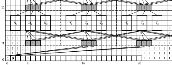
Figure 2: Illustration of the approach of how to succinctly encode a Boolean circuit encoding the computation table of a polynomial-time Turing machine on an input of exponential size. Each square represents a gate, all gates not surrounded by boxes are assumed to be gates with constant value 1.

In the next section, for our lower bound we will apply Lemma 1, which entails deciding $(w,w_{1},\ldots,w_{i})\in R$, where the $w_{j}$ are of size exponential in $n=\lvert w\rvert$. Let $M_{w}$ be a polynomial-time Turing machine deciding $R$ for a fixed $w$. The $w_{1},\ldots w_{j}$ will implicitly be coded into natural numbers, so it will not be possible to construct a Boolean circuit $\mathcal{C}_{w}$ upfront that can evaluate $M_{w}$ on the input $w_{1},\ldots w_{j}$ of exponential size, since we are required to establish a polynomial-time reduction. Instead, we will succinctly encode $\mathcal{C}_{w}$ via another Boolean circuit $\mathcal{D}_{w}$. More precisely, $\mathcal{C}_{w}$ is encoded via $\mathcal{D}_{w}$ as follows: $\mathcal{D}_{w}$ has $3r(n)+3$ input gates for some fixed polynomial $r$ depending on $M_{w}$ such that for $i,j,k\in[2^{r(n)}]$ and $t\in[5]$, $\mathcal{D}_{w}(t,i,j,k)=1$ iff the defining function $f$ of $\mathcal{C}_{w}$ gives $f(i)=(t,j,k)$, i.e., that the gate with index $i$ of $\mathcal{C}_{w}$ is of type $t$ and has input gates with index $j$ and $k$. In particular, $\mathcal{D}_{w}$ and henceforth $\mathcal{C}_{w}$ only depend on $w$ and $M$, and are independent of $w_{1},\ldots w_{i}$. Note that we can view an assignment of truth values to the gates of $\mathcal{C}_{w}$ as a string of length $2^{r(n)}$.

More generally, it is known that if $\mathcal{C}$ with no input gates is succinctly given by some circuit $\mathcal{D}$, determining whether $\mathcal{C}$ evaluates to true is $\EXP$-complete [Pap94, , Thm. 20.2 & Cor. 2]. The idea underlying the hardness proof is a straight-forward generalisation of the approach outlined in the paragraph above. The circuit $\mathcal{C}$ encodes the computation table of an $\EXP$ Turing machine $M$. Since the indices of the gates of $\mathcal{C}$ can be represented in binary, via $\mathcal{D}$ we can encode $\mathcal{C}$ by implicitly encoding an exponential number of the constant basic circuit ensuring proper propagation between consecutive cells. This approach can now be adapted for our purpose, i.e., to evaluate a polynomial-time Turing machine on an input of exponential size. The major challenge is to transfer input to the succinctly encoded circuit on-the-fly.

Referring to Lemma 1 and given $M_{w}$ as above, we can construct in logarithmic space a Boolean circuit $\mathcal{D}_{w}$ encoding $\mathcal{C}_{w}$ such that the input $(w_{1},\ldots,w_{i})$ to $\mathcal{C}_{w}$ is obtained from the first $i2^{q(n)}$ gates, and $\mathcal{C}_{w}$ encodes a computation table of $M_{w}$ on this input. Figure 2 illustrates how this can be realised. Each box in Figure 2 is a gate, and a cell of the computation table of $M_{w}$ while being executed on $(w_{1},\ldots,w_{n})$ is encoded into the dashed boxes, or more specifically, into the three framed gray-shaded boxes on the bottom of the dashed boxes. Here, we assume that three bits are sufficient to represent the alphabet of the computation table of $M_{w}$, and that $\triangleright_{q_{0}}$ is encoded as $111$. Consequently, the gates with index $(3,4),(3,5)$ and $(3,6)$, representing the cell $T_{1,1}$ of the computation table of $M_{w}$, are gates with constant value one, as indicated in Figure 2. Now we want the values of the cells $T_{1,2}$, $T_{1,3}$, etc. of the computation table of $M_{w}$ to be equivalent to $w_{1}\cdots w_{n}$, which are represented by the gates with indices $(0,0),\ldots(0,i2^{q(n)})$. The gates in $\mathcal{D}_{w}$ corresponding to $T_{1,2}$ and $T_{1,3}$ have indices $(3,15),(3,16),(3,17)$ and $(3,26),(3,27),(3,28)$, respectively. Those gates have the gates $(0,0)$ and $(0,1)$ as their inputs, respectively. Suppose that in our encoding $1$ is represented as $101$ and $0$ as $010$, the sequence of $\|$, $\sim$ and $\|$ gates ensures that $1$ is mapped to $101$ and $0$ to $010$. Consequently, the gates $(3,15),(3,16),(3,17)$ can correctly transfer the alphabet symbols $\{0,1\}$ of $M_{w}$ into the internal representation of the computation table, and in particular copy the first symbol of the input string $w_{1}\cdots w_{i}$ into the internal representation of the computation table. In the example in Figure 2, the gates with index $(3,15),(3,16),(3,17)$ would output $1$, $0$ and $1$, respectively, since the gate $(0,0)$ has value $1$ which corresponds to the first symbol of the input string $w_{1}$. As stated before, in our reduction this value is provided on-the-fly. The rest of the reduction follows standard arguments. Each dashed box contains circuits $\mathcal{T}_{1},\mathcal{T}_{2}$ and $\mathcal{T}_{3}$ which compute the consecutive cell of the simulated computation table of $M_{w}$, i.e., the values of the three gates representing this cell. The dashed boxes on the left use different circuits $\mathcal{U}_{1},\mathcal{U}_{2}$ and $\mathcal{U}_{3}$ since they do not have a left neighbor. All unused gates can assumed to be dummy gates, i.e. gates with constant value $1$, as indicated in Figure 2. It follows that $M_{w}$ accepts $(w_{1},\ldots,w_{i})$ iff $\mathcal{C}_{w}$ evaluates to true on the input provided, i.e., the value of the gate with the highest index of $\mathcal{C}_{w}$ is equal to 1.

In order to encode $\mathcal{C}_{w}$ succinctly, it is clear that due to the regular structure of $\mathcal{C}_{w}$, the type and input gates to any gate can be computed from a given index of a gate by a polynomial-time algorithm. The circuit $\mathcal{D}_{w}$ can now be taken as the circuit corresponding to this algorithm.

3 Completeness of the $\Sigma_{i+1}$-Fragment of Presburger Arithmetic for $\mathsf{\Sigma}_{i}^{\EXP}$

In this section, we show that PA($i+1$) is $\mathsf{\Sigma}_{i}^{\EXP}$-complete for every fixed $i>0$. We begin with the lower bound and first note that it is not possible to adapt Berman’s hardness proof Ber80 in order to get the desired result, since it relies on a trick by Fischer & Rabin FR74 in order to perform arithmetic operations on a bounded interval over large numbers which linearly increases the number of quantifier alternations. Instead, we will partly adapt concepts and ideas introduced by Grädel in his hardness proof for PA($2$) in Grae89 and Gottlob, Leone & Veith in GLV95 . Roughly speaking, we aim for “implementing” Lemma 1 via a PA($i+1$) formula, which will entail encoding bit strings of exponential size into natural numbers and evaluating Boolean circuits in Presburger arithmetic on-the-fly. The upper bound does not follow immediately and requires combining solution intervals established by Weispfenning in Wei90 with Proposition 4.

3.1 Lower Bounds

The goal of this section is to prove the following proposition.

Proposition 6.

Let $L\subseteq\{0,1\}^{*}$ be a language in $\mathsf{\Sigma}_{i}^{\EXP}$, $i>0$ and $w\in\{0,1\}^{*}$. There exists a polynomial-time computable PA($i+1$) formula $\Phi_{L,w}$ such that $w\in L$ iff $\Phi_{L,w}$ is valid.

To this end, we employ the characterisation of $\mathsf{\Sigma}_{i}^{\EXP}$ in Lemma 1. Let $M$ be the deterministic polynomial-time Turing machine deciding $R$ from Lemma 1, and let $M_{w}$ be such a Turing machine deciding $R$ for a fixed input $w\in\{0,1\}^{n}$, which can be computed from $M$ in logarithmic space. The bit strings $w_{1}$ to $w_{i}$ from Lemma 1 constituting the input to $M_{w}$ are represented in our reduction via natural numbers assigned to first-order variables $\mathbf{x}=(x_{1},\ldots,x_{i})$. The precise encoding of a $w_{j}$ via $x_{j}$ is discussed below. For now, it is only important to mention that not every natural number encodes a bit string. Let us focus on the high-level structure of $\Phi_{L,w}$:

$$\Phi_{L,w}\stackrel{{\scriptstyle\text{def}}}{{=}}\exists x_{1}.\forall x_{2}\cdots Q_{i}x_{i}.\bigwedge_{1\leq j\leq i,~{}j\text{ odd}}\Psi_{\mathit{valid,r(n)}}(x_{j})\wedge\\ \wedge\Big{(}\bigwedge_{1\leq j\leq i,~{}j\text{ even}}\Psi_{\mathit{valid},r(n)}(x_{j})\Big{)}\rightarrow\Psi_{M_{w}}(x_{1},\ldots,x_{i}).$$ (1)

Unsurprisingly, the alternation of quantifiers in Lemma 1 is reflected by the alternation of quantifiers in (1), so $Q_{i}=\exists$ if $i$ is odd and $Q_{i}=\forall$ if $i$ is even. The formula $\Psi_{\mathit{valid},r(n)}(x_{i})$ is a $\Pi_{1}$-formula, and $\Psi_{M_{w}}(x_{1},\ldots,x_{i})$ is a formula in the Boolean closure of $\Sigma_{1}$ if $i$ is odd and a $\Sigma_{1}$-formula if $i$ is even. The first conjunct ensures that the existentially quantified variables represent encodings of bit strings and the second conjunct that, under the additional assumption that the universally quantified variables encode valid bit strings as well, $M_{w}$ accepts the bit strings encoded in $x_{1},\ldots,x_{i}$. For the given $w\in\{0,1\}^{n}$, those formulas are concrete instances of a family of formulas, and $r(n)$ is an index in this family for some polynomial $r(n)$ which dominates $q(n)$ in Lemma 1 and is made more precise at a later stage. Consequently, for a fixed $i>0$, we have that $\Phi_{L,w}$ is a PA($i+1$) formula.

In our reduction, we have to take extra care to prevent the “accidental” introduction of quantifier alternations. In general when providing formulas, we adapt Grädel’s approach in Grae89 and provide neutral formulas, which are open polynomially equivalent $\Sigma_{1}$- and $\Pi_{1}$-formulas. This ensures that, for instance, we do not have to care about whether we could possibly introduce a new quantifier alternation if a formula is used on the left-hand side of an implication. When providing a neutral $\Sigma_{1}$-formula $\Phi(\mathbf{x})=\exists\mathbf{y}.\varphi(\mathbf{x},\mathbf{y})$, we will denote by $\bar{\Phi}(\mathbf{x})=\forall\mathbf{y}.\bar{\varphi}(\mathbf{x},\mathbf{y})$ its neutral equivalent $\Pi_{1}$ counterpart. For the sake of consistent naming, whenever $\Phi(\mathbf{x})$ occurs as a subformula in some other formula, we implicitly assume that it is appropriately replaced such that the resulting formula is either a $\Sigma_{1}$- or a $\Pi_{1}$-formula, depending on the context. Likewise, if for instance $\Phi(\mathbf{x})$ occurs as a negated subformula in a formula that is supposed to be existentially quantified, we assume that this subformula is implicitly replaced by $\exists\mathbf{x}.\neg(\bar{\varphi}(\mathbf{x},\mathbf{y}))$, and $\neg(\bar{\varphi}(\mathbf{x},\mathbf{y}))$ is treated in the same way if it is not yet quantifier-free. In this way, we can always make sure to result in $\Sigma_{1}$- or $\Pi_{1}$-formulas.

We now turn towards the details of our reduction and begin with discussing the encoding of bit strings as natural numbers we use subsequently. The encoding we use is due to Grädel Grae89 . In his $\NEXP$ lower bound for PA($2$) he exploits a result due to Ingham Ing40 ; Che10 that for any sufficiently large $i\in\mathbb{N}$ there is at least one prime in the interval $[i^{3},(i+1)^{3})$. Given a bit string $w=b_{1}\cdots b_{n}\in\{0,1\}^{n}$, a natural number $a\in\mathbb{N}$ encodes $w$ if for all $1\leq i\leq n$ and

$$\text{for all primes }p\in[i^{3},(i+1)^{3}):a\equiv b_{i}\bmod p.$$

The existence of such an $a$ is then guaranteed by the Chinese remainder theorem. Given a fixed $n>0$, we call $a\in\mathbb{N}$ a valid encoding if for every $1\leq i\leq n$, either $a\equiv 0\bmod p$ or $a\equiv 1\bmod p$ for all prime numbers $p\in[i^{3},(i+1)^{3})$.

In order to enable the extraction of bits of bit strings encoded as naturals, we show how to check for divisibility with a natural number whose number of bits is fixed. Next, we show how to evaluate a Boolean circuit in Presburger arithmetic. This serves two purposes: first, it allows for deciding if a given number lies in an interval $[i^{3},(i+3)^{3})$ and for testing whether a given number is a prime due to the AKS primality test AKS02 . Second, it allows for simulating $M_{w}$ discussed above on an input of exponential size using its succinct encoding via a circuit as discussed in Section 2.5. Putting everything together eventually yields the desired reduction.

We begin with a family of quantifier-free formulas $\Phi_{\mathit{bin},n}(\mathbf{x},x)$ such that given $\mathbf{b}\in\{0,1\}^{n}$ and $b\in\mathbb{N}$, $\Phi_{\mathit{bin},n}(\mathbf{b},b)$ holds if $\mathbf{b}$ is the binary representation of $b$. Consequently, this formula implicitly constraints $b$ such that $b\in[2^{n}]$:

$$\Phi_{\mathit{bin},n}(\mathbf{x},x) \stackrel{{\scriptstyle\text{def}}}{{=}}\bigwedge_{i\in[n]}(x_{i}=0\vee x_{i}=1)\wedge x=\sum_{i\in[n]}2^{i}x_{i}.$$ (2)

Next, we provide a family of neutral formulas $\Phi_{\mathit{mod},n}(x,y)$ such that for $a,b$ with $b\in[2^{n}]$, $\Phi_{\mathit{mod},n}(a,b)$ holds iff $a\equiv 0\bmod b$. Essentially, $\Phi_{\mathit{mod},n}(x,y)$ realises a formula for bounded multiplication. In contrast to a formula with the same purpose given in Grae89 , it is not recursively defined and of size $O(n)$ as opposed to $O(n\log n)$ when binary encoding of numbers is assumed. The latter fact will be useful in Section 4. The underlying idea of the subsequent definitions is that if the binary expansion of $b$ is $b=\sum_{i\in[n]}2^{i}b_{i}~{}\text{and}~{}bk=a$ for some $k\geq 0$ then $a$ can be written as $a=\sum_{i\in[n]}2^{i}a_{i}$ with $a_{i}=kb_{i}$:

$$\Phi_{\mathit{dig},n}(\mathbf{x},\mathbf{y},k) \stackrel{{\scriptstyle\text{def}}}{{=}}\bigwedge_{i\in[n]}(y_{i}=0\rightarrow x_{i}=0\wedge y_{i}=1\rightarrow x_{i}=k)$$

$$\Phi_{\mathit{mod},n}(x,y) \stackrel{{\scriptstyle\text{def}}}{{=}}\exists\mathbf{x}.\exists\mathbf{y}.\exists k.\Phi_{\mathit{bin},n}(\mathbf{y},y)\wedge$$

$$~{}~{}~{}~{}~{}~{}~{}~{}\wedge\Phi_{\mathit{dig},n}(\mathbf{x},\mathbf{y},k)\wedge x=\sum_{i\in[n]}2^{i}x_{i}$$ (3)

$$\bar{\Phi}_{\mathit{mod},n}(x,y) \stackrel{{\scriptstyle\text{def}}}{{=}}\forall\mathbf{x}.\forall\mathbf{y}.\forall k.\big{(}\Phi_{\mathit{bin},n}(\mathbf{y},y)\wedge$$

$$~{}~{}~{}~{}~{}~{}\wedge\Phi_{\mathit{dig},n}(\mathbf{x},\mathbf{y},k)\big{)}\rightarrow x=\sum_{i\in[n]}2^{i}x_{i}.$$

We now turn towards evaluating Boolean circuits with suitable formulas in Presburger arithmetic. The subsequent formulas for evaluating a circuit $\mathcal{C}$ with $n$ input and $r$ gates in total are essentially an adaption of a construction given by Gottlob, Leone & Veith in GLV95 . It is easily checked that for $a\in[2^{n}]$, $\Phi_{\mathcal{C}}(a)$ holds iff $\mathcal{C}(a)=1$. In $\Phi_{\mathcal{C}}$, the input to $\mathcal{C}$ is encoded via a dimension $n$ vector of first-order variables $\mathbf{x}$ and the Boolean assignment to the gates via a dimension $r$ vector of first-order variables $\mathbf{y}$, which are implicitly assumed to range over $\{0,1\}$. First, we provide a formula ensuring that the structure of the gates of $\mathcal{C}$ is correctly encoded in $\mathbf{y}$:

$$\Phi_{\mathcal{C},\mathit{gates}}(\mathbf{x},\mathbf{y})\stackrel{{\scriptstyle\text{def}}}{{=}}\\ \bigwedge_{i\in[r]}\left\{\begin{array}[]{ll}y_{i}=1\leftrightarrow(y_{j}=1\wedge y_{k}=1)&\text{if }f(i)=(\&,j,k)\\ y_{i}=1\leftrightarrow(y_{j}=1\vee y_{k}=1)&\text{if }f(i)=(\|,j,k)\\ y_{i}=1\leftrightarrow y_{j}=0&\text{if }f(i)=({\sim},j,k)\\ y_{i}=x_{i}&\text{if }f(i)=(\uparrow,0,0)\\ y_{i}=1&\text{if }f(i)=(\downarrow_{1},0,0).\end{array}\right.$$ (4)

Next, the formula $\Phi_{\mathcal{C}}(x)$ defined below now enables us to determine whether $\mathcal{C}$ accepts a given input encoded into the first-order variable $x$:

$$\Phi_{\mathcal{C}}(x) \stackrel{{\scriptstyle\text{def}}}{{=}}\begin{aligned} \exists\mathbf{x}.\exists\mathbf{y}.\exists y.\Phi_{\mathit{bin},n}(\mathbf{x},x)\wedge\Phi_{\mathit{bin},r}(\mathbf{y},y)\wedge\\ \wedge\Phi_{\mathcal{C},\mathit{gates}}(\mathbf{x},\mathbf{y})\wedge y_{r}=1\end{aligned}$$ (5)

$$\bar{\Phi}_{\mathcal{C}}(x) \stackrel{{\scriptstyle\text{def}}}{{=}}\begin{aligned} \forall\mathbf{x}.\forall\mathbf{y}.\forall y.\big{(}\Phi_{\mathit{bin},n}(\mathbf{x},x)\wedge\Phi_{\mathit{bin},r}(\mathbf{y},y)\wedge\\ \wedge\Phi_{\mathcal{C},\mathit{gates}}(\mathbf{x},\mathbf{y})\big{)}\rightarrow y_{r}=1.\end{aligned}$$ (6)

We now show how a predicate determining whether a given number $a\in\mathbb{N}$ is a prime number in the interval $[b^{3},(b+1)^{3})$ for some $b>0$ representable by $n$ bits can be realised. It is easily verified that any number in this interval can be represented by at most $m=3(n+1)$ bits. Moreover as discussed above, both conditions can be decided in polynomial time. Therefore we can construct in logarithmic space a Boolean circuit $\mathcal{C}_{\mathit{prime},n}$ with $m+n$ input gates implementing this predicate [Pap94, , Thm. 8.1] and define

$$\Phi_{\mathit{prime},n}(x,y)\stackrel{{\scriptstyle\text{def}}}{{=}}\exists\mathbf{x}.\exists\mathbf{y}.\exists z.\Phi_{\mathit{bin},m}(\mathbf{x},x)\wedge\Phi_{\mathit{bin},n}(\mathbf{y},y)\wedge\\ \wedge z=\sum_{i\in[m]}2^{i}x_{i}+2^{m}\sum_{i\in[n]}2^{i}y_{i}\wedge\Phi_{\mathcal{C}_{\mathit{prime},n}}(z)$$ (7)

$$\bar{\Phi}_{\mathit{prime},n}(x,y)\stackrel{{\scriptstyle\text{def}}}{{=}}\forall\mathbf{x}.\forall\mathbf{y}.\forall z.\big{(}\Phi_{\mathit{bin},m}(\mathbf{x},x)\wedge\Phi_{\mathit{bin},n}(\mathbf{y},y)\wedge\\ \wedge z=\sum_{i\in[m]}2^{i}x_{i}+2^{m}\sum_{i\in[n]}2^{i}y_{i}\big{)}\rightarrow\Phi_{\mathcal{C}_{\mathit{prime},n}}(z).$$ (8)

The first line of $\Phi_{\mathit{prime},n}(x,y)$ converts $x$ and $y$ into their binary representation. Next, the second line first concatenates these bit representations via the additional variable $z$ by appropriately shifting the value of $y$ by $m$ bits, and finally $z$ is passed to $\mathcal{C}_{\mathit{prime},n}$. Consequently, we have that $\Phi_{\mathit{prime},n}(a,b)$ holds iff $a$ is prime and $a\in[b^{3},(b+1)^{3})$.

We are now in a position in which we can define a family of $\Pi_{1}$-formulas $\Psi_{\mathit{valid},n}(x)$ used in (1) that allow for testing whether some $a\in\mathbb{N}$ represents a valid respectively invalid encoding of a bit string of length $2^{n}$. For valid encodings, we wish to make sure that all primes in every relevant interval $[b^{3},(b+1)^{3})$ have uniform residue classes in $a$ for all $1\leq b\leq 2^{n}$, i.e., for any two primes $p_{1},p_{2}\in[b^{3},(b+1)^{3})$ we either have $a\equiv 0\textrm{ mod }p_{1}$ and $a\equiv 0\textrm{ mod }p_{2}$, or $a-1\equiv 0\textrm{ mod }p_{1}$ and $a-1\equiv 0\textrm{ mod }p_{2}$. Let $m$ be as above,

$$\Psi_{\mathit{valid},n}(x)\stackrel{{\scriptstyle\text{def}}}{{=}}\forall y.\forall p_{1}.\forall p_{2}.\big{(}1\leq y\leq 2^{n}\wedge\\ \wedge\Phi_{\mathit{prime},{n+1}}(p_{1},y)\wedge\Phi_{\mathit{prime},{n+1}}(p_{2},y)\big{)}\rightarrow\\ \rightarrow\big{(}(\Phi_{\mathit{mod},m+3}(x,p_{1})\wedge\Phi_{\mathit{mod},m+3}(x,p_{2}))\vee\\ \vee(\Phi_{\mathit{mod},m+3}(x-1,p_{1})\wedge\Phi_{\mathit{mod},m+3}(x-1,p_{2}))\big{)}.$$

In order to complete our hardness proof for $\mathsf{\Sigma}_{i}^{\EXP}$ for a subsequently fixed $i>0$ via its characterisation in Lemma 1 and $\Phi_{L,w}$ in (1), we will now define the remaining $\Pi_{1}$-formula $\Psi_{M_{w}}(x_{1},\ldots,x_{i})$ for a given $w\in\{0,1\}^{n}$. Let $\mathcal{C}_{w}$ be the Boolean circuit succinctly encoded by a Boolean circuit $\mathcal{D}_{w}(t,y,z_{1},z_{2})$ deciding $M_{w}$ on an input of length $2^{q(n)}i$ such that $\mathcal{C}_{w}$ consists of $2^{r(n)}$ gates for some polynomial $r:\mathbb{N}\to\mathbb{N}$. Recall that we can view an assignment of truth values to the gates of the succinctly encoded circuit $\mathcal{C}_{w}$ as a bit string, or sequence of bit strings, of appropriate length. In the following let $\mathbf{a}=(a_{1},\ldots,a_{i})\in\mathbb{N}^{i}$ be a valuation, for any $1\leq j<i$ each $a_{j}$ will be used to encode the values of the input gates with index $2^{q(n)}(j-1)$ up to $2^{q(n)}j-1$ of $\mathcal{C}_{w}$, and $a_{i}$ will encode the values of the gates with index $2^{q(n)}(i-1)$ up to the gate with index $2^{r(n)}-1$ of $\mathcal{C}_{w}$. So in particular the internal gates of $\mathcal{C}_{w}$ are encoded in $a_{i}$.

In order to extract encodings of bit strings from natural numbers, as a first step we provide neutral formulas $\Phi_{\mathcal{C}_{w},0}(x,y)$ and $\bar{\Phi}_{\mathcal{C}_{w},0}(x,y)$ which assume $x$ to be a valid encoding. These formulas enable us to test whether a bit of a bit string whose index is given by $y$ is encoded to be zero in $x$. Formally, for a valid encoding $a\in\mathbb{N}$ and for $b\in[2^{r(n)}]$, we have $\Phi_{\mathcal{C}_{w},0}(a,b)$ iff there is a prime $p\in[(b+1)^{3},(b+2)^{3})$ and $a\equiv 0\bmod p$, or $a\equiv 0\bmod p$ for all primes $p\in[(b+1)^{3},(b+2)^{3})$, respectively. Let $r^{\prime}(x)=r(x)+1$, we define:

$$\Phi_{\mathcal{C}_{w},0}(x,y) \stackrel{{\scriptstyle\text{def}}}{{=}}\exists p.\Phi_{prime,r^{\prime}(n)}(p,y+1)\wedge\Phi_{\mathit{mod},r^{\prime}(n)}(x,p)$$

$$\bar{\Phi}_{\mathcal{C}_{w},0}(x,y) \stackrel{{\scriptstyle\text{def}}}{{=}}\forall p.\Phi_{prime,r^{\prime}(n)}(p,y+1)\rightarrow\Phi_{\mathit{mod},r^{\prime}(n)}(x,p).$$

The formulas $\Phi_{\mathcal{C}_{w},1}(x,y)$ and $\bar{\Phi}_{\mathcal{C}_{w},1}(x,y)$ testing whether the bit with index $y$ is set to 1 in the encoding $x$ can be defined analogously by negating $\Phi_{\mathcal{C}_{w},0}(x,y)$. The previously constructed formulas now enable us to define formulas that allow for evaluating the succinctly encoded $\mathcal{C}_{w}$ on an input that is provided on-the-fly via $\mathbf{a}$. Given an index $b$ implicitly less than $2^{r(n)}$ of a gate of $\mathcal{C}_{w}$, represented by the first-order variable $y$, and a vector of valid encodings $\mathbf{a}=(a_{1},\ldots,a_{i})$ represented by the first-order variables $\mathbf{x}$, the following formula $\Phi_{\mathcal{C}_{w},\top}(\mathbf{x},y)$ checks whether the value of the gate with index $b$ is set to true under the valuation $\mathbf{a}$ according to the convention described before:

$$\Phi_{\mathcal{C}_{w},\top}(\mathbf{x},y)\stackrel{{\scriptstyle\text{def}}}{{=}}\bigwedge_{1\leq j<i}\Big{(}\big{(}2^{q(n)}(j-1)\leq y<2^{q(n)}j\rightarrow\\ \rightarrow\Phi_{\mathcal{C}_{w},1}(x_{j},y)\big{)}\wedge\big{(}2^{q(n)}(i-1)\leq y\rightarrow\Phi_{\mathcal{C}_{w},1}(x_{i},y)\big{)}\Big{)}.$$

A formula $\Phi_{\mathcal{C}_{w},\bot}(\mathbf{x},y)$ testing whether the value of a gate is set to false can be defined analogously by negating $\Phi_{\mathcal{C}_{w},\top}(\mathbf{x},y)$. Building upon those formulas, we can now construct Boolean connectives that allow for checking that the gates of $\mathcal{C}_{w}$ are consistently encoded. Given $\mathbf{a}\in\mathbb{N}^{i}$ as above, $\Phi_{\mathcal{C}_{w},\&}(\mathbf{a},b,c_{1},c_{2})$ holds if the logical and-connective holds for the truth values of the gates with index $b,c_{1}$ and $c_{2}$ encoded via $\mathbf{a}$:

$$\Phi_{\mathcal{C}_{w},\&}(\mathbf{x},y,z_{1},z_{2})=\\ \big{(}\Phi_{\mathcal{C}_{w},\top}(\mathbf{x},y)\leftrightarrow\Phi_{\mathcal{C}_{w},\top}(\mathbf{x},z_{1})\wedge\Phi_{\mathcal{C}_{w},\top}(\mathbf{x},z_{2})\big{)}.$$

The remaining Boolean connectives found in Definition 1 can be reflected via the additional formulas

$$\Phi_{\mathcal{C}_{w},\|}(\mathbf{x},y,z_{1},z_{2}),~{}\Phi_{\mathcal{C}_{w},\sim}(\mathbf{x},y,z_{1},z_{2})\text{ and }\Phi_{\mathcal{C}_{w},\downarrow_{1}}(\mathbf{x},y,z_{1},z_{2})$$

which are defined analogously to $\Phi_{\mathcal{C}_{w},\&}(\mathbf{x},y,z_{1},z_{2})$. These formulas now enable us to define a $\Pi_{1}$-analogue to $\Phi_{\mathcal{C},\mathit{gates}}(\mathbf{x},\mathbf{y})$ in (4) in order to check if the Boolean assignment of the succinctly encoded circuit $\mathcal{C}_{w}$ is consistent:

$$\Psi_{\mathcal{C}_{w},\mathit{gates}}(\mathbf{x})=\forall t.\forall y.\forall z_{1}.\forall z_{2}.\Phi_{\mathcal{D}_{w}}(t,y,z_{1},z_{2})\rightarrow\\ \rightarrow\bigwedge\left\{\begin{array}[]{l}t=0\rightarrow\Phi_{\mathcal{C}_{w},\&}(\mathbf{x},y,z_{1},z_{2})\\ t=1\rightarrow\Phi_{\mathcal{C}_{w},\|}(\mathbf{x},y,z_{1},z_{2})\\ t=2\rightarrow\Phi_{\mathcal{C}_{w},\top}(\mathbf{x},y)\leftrightarrow\Phi_{\mathcal{C}_{w},\bot}(\mathbf{x},z_{1})\\ t=4\rightarrow\Phi_{\mathcal{C}_{w},\top}(\mathbf{x}).\end{array}\right.$$

Here, $\Phi_{\mathcal{D}_{w}}(t,y,z_{1},z_{2})$ is an instantiation of $\Phi_{\mathcal{C}}(x)$ defined in (5) and (6) for the circuit $\mathcal{D}_{w}$. The use of $\Phi_{\mathcal{D}_{w}}(t,y,z_{1},z_{2})$ is not totally clean as $\Phi_{\mathcal{C}}(x)$ it is only open in $x$. However, this can easily be fixed by concatenating $t,y,z_{1}$ and $z_{2}$ into a single first-order variable as it was done in (7) and (8), and details have only been omitted for the sake of readability. Also note that the values of $t,y,z_{1}$ and $z_{2}$ are then implicitly bounded through $\Phi_{\mathcal{D}_{w}}(t,y,z_{1},z_{2})$.

Finally, we can define $\Psi_{M_{w}}(x_{1},\ldots,x_{i})$, the last remaining formula from (1), as follows

$$\Psi_{M_{w}}(x_{1},\ldots,x_{i})\stackrel{{\scriptstyle\text{def}}}{{=}}\\ \left\{\begin{array}[]{ll}\Psi_{\mathcal{C}_{w},\mathit{gates}}(\mathbf{x})\wedge\Phi_{\mathcal{C}_{w},\top}(\mathbf{x},2^{r(n)}-1)&\text{ if }i\text{ is odd}\\ \Psi_{\mathcal{C}_{w},\mathit{gates}}(\mathbf{x})\rightarrow\Phi_{\mathcal{C}_{w},\top}(\mathbf{x},2^{r(n)}-1)&\text{ if }i\text{ is even}\end{array}\right.$$

Inspecting the construction outlined in this section, it is not difficult to see that for a given $w\in\{0,1\}^{n}$ the construction of $\Phi_{L_{w}}(x_{1},\ldots,x_{i})$ is tedious, but can be performed in polynomial time with respect to $n$. We leave it as an open problem whether this reduction can actually be performed in logarithmic space, though there do not seem to be any major obstacles. Following the argumentation of this section, we conclude that $\Phi_{L,w}$ is the formula required in Proposition 6.

3.2 Upper Bounds

We will now show that the previously obtained lower bounds have corresponding upper bounds. Let us first recall an improved version of a result by Reddy & Loveland RL78 established by Weispfenning [Wei90, , Thm. 2.2], which bounds the solution intervals of Presburger formulas.

Proposition 7 (Weispfenning Wei90 ).

There exists a constant $c>0$ such that for any PA($i$,$j$) formula $\Phi$ and $N=\{0,\ldots 2^{c|\Phi|^{(3j)^{i}}}\}$, $\Phi$ is valid iff $\Phi$ is valid when restricting the first-order variables of $\Phi$ to be interpreted over elements from $N$.

Together with Lemma 1, this immediately gives that for any fixed $i>0$, validity in PA($i+1$) is in $\mathsf{\Sigma}_{i+1}^{\EXP}$. We now show how to decrease the number of oracle calls by one.

To this end, let $\Phi$ be a PA($i+1$,$j$) formula in prenex normal form for a fixed $i>0$ and some $j$, i.e.,

$$\Phi=\exists\mathbf{x}_{1}.\forall\mathbf{x}_{2}\cdots Q_{i+1}\mathbf{x}_{i+1}.\varphi(\mathbf{x}_{1},\ldots,\mathbf{x}_{i+1}).$$

In order to decide validity of $\Phi$, by application of Proposition 7, a $\mathsf{\Sigma}_{i}^{\EXP}$-algorithm can alternatingly guess valuations $\mathbf{a}_{1},\ldots\mathbf{a}_{i}\in\mathbb{N}^{j}$ for the $\mathbf{x}_{1},\ldots\mathbf{x}_{i}$ such that $\lVert\mathbf{a}_{k}\rVert\leq 2^{c\lvert\Phi\rvert^{(3j)^{i+1}}}$ for all $1\leq k\leq i$ and some constant $c>0$, and by additionally padding valuations with leading zeros, we may assume that any number in every $\mathbf{a}_{k}$ is represented using $2^{\poly(\lvert\Phi\rvert)}$ bits. Consequently, it remains to show that validity of $Q_{i+1}\mathbf{x}_{i+1}.\varphi(\mathbf{a}_{1}/\mathbf{x}_{1},\ldots,\mathbf{a}_{i}/\mathbf{x}_{i},\mathbf{x}_{i+1})$ can be decided in polynomial time. This is, of course, not the case under standard assumptions from complexity theory. However, the final call to the $\mathsf{\Sigma}_{0}^{\P}$-oracle of a $\mathsf{\Sigma}_{i}^{\EXP}$ algorithm gets $\varphi$ and all $\mathbf{a}_{k}$ as input, the latter being of exponential size in $\lvert\Phi\rvert$. Informally speaking, this provides us with sufficient additional time in order to decide validity of

$$Q_{i+1}\mathbf{x}_{i+1}.\varphi(\mathbf{a}_{1}/\mathbf{x}_{1},\ldots,\mathbf{a}_{i}/\mathbf{x}_{i},\mathbf{x}_{i+1})$$ (9)

in polynomial time with respect to the size of the input.

1:  $\varphi(\mathbf{x}_{1},\ldots,\mathbf{x}_{i+1}):=$DNF$(\varphi(\mathbf{x}_{1},\ldots,\mathbf{x}_{i+1}))$

2:  for all clauses $\psi(\mathbf{x}_{1},\ldots,\mathbf{x}_{i+1})$ of $\varphi$ do

3:     for all literals $t=p(\mathbf{x}_{1},\ldots,\mathbf{x}_{i+1})<b$ of $\psi$ do

4:        replace $t$ in $\psi$ with $-p(\mathbf{x}_{1},\ldots,\mathbf{x}_{i+1})\geq-b+1$

5:     end for

6:     for all literals $t=\neg(p(\mathbf{x}_{1},\ldots,\mathbf{x}_{i+1})<b)$ do

7:        replace $t$ in $\psi(\mathbf{x}_{1},\ldots,\mathbf{x}_{i+1})$ with $p(\mathbf{x}_{1},\ldots,\mathbf{x}_{i+1})\geq b$

8:     end for

9:     $(S:A\mathbf{x}_{i+1}\geq\mathbf{c}):=\psi[\mathbf{a}_{1}/\mathbf{x}_{1},\ldots,\mathbf{a}_{i}/\mathbf{x}_{i}]$

10:     if $\llbracket S\rrbracket\neq\emptyset$ then

11:        return  true

12:     end if

13:  end for

14:  return  false

Algorithm 1 Deciding $\exists\mathbf{x}_{i+1}.\varphi(\mathbf{x}_{1},\ldots,\mathbf{x}_{i+1})$ for a given instantiation $\mathbf{a}_{1},\ldots\mathbf{a}_{i}\in\mathbb{N}^{j}$ of $\mathbf{x}_{1},\ldots\mathbf{x}_{i}$.

Algorithm 1, which takes $\varphi$ and the $\mathbf{a}_{k}$ as input, is a pseudo algorithm deciding validity of a formula as in (9) for even $i$, i.e., $Q_{i+1}=\exists$. The case $Q_{i+1}=\forall$ can be derived symmetrically. Let us discuss Algorithm 1 and analyse its running time. In Line 1, the algorithm converts $\varphi$ into disjunctive normal form. This step can be performed in exponential time $\DTIME(2^{O(\lvert\Phi\rvert)})$ and thus takes polynomial time with respect to the input. Starting in Line 2, the algorithm iterates over all clauses $\psi$ of $\varphi$, and since there are at most $2^{O(\lvert\Phi\rvert)}$ clauses this iteration is performed at most a polynomial number of times with respect to the size of the input. In each iteration, in Lines 3–8 the algorithm transforms the disjuncts of $\psi$ into linear inequalities by eliminating negation. After Line 8, $\psi$ is a conjunction of linear inequalities and thus gives rise to an equivalent system of linear Diophantine inequalities $S$ in which the first-order variables $\mathbf{x}_{1},\ldots\mathbf{x}_{i}$ are instantiated by the $\mathbf{a}_{1},\ldots\mathbf{a}_{i}$. Clearly, Lines 3–9 can be executed in polynomial time with respect to the size of the input. Finally, in Line 10 feasibility of $S$ is checked. To this end, we invoke Proposition 4 from which it follows that feasibility of each $S$ can be decided in $\DTIME(2^{p(\lvert\Phi\rvert)}\lvert S\rvert)$ for some polynomial $p$. This step is again polynomial with respect to the input to the oracle call. If $S$ is feasible the algorithm returns true in Line 11. Otherwise, if no $S$ is feasible for all disjuncts of $\varphi$, the algorithm returns false in Line 14. Consequently, we have shown the following proposition, which together with Proposition 6 completes the proof of Theorem 1.

Proposition 8.

For any fixed $i>0$, PA($i+1$) is decidable in $\mathsf{\Sigma}_{i}^{\EXP}$.

3.3 Discussion

We conclude this part of the paper with a short discussion on the relationship of our proof of the lower bound of PA(${i+1}$) to the proof of a $\NEXP$ lower bound for PA($2$) by Grädel Grae89 , and applications of and results derivable from Proposition 8.

As it emerged in Section 3.1, at many places we can apply and reuse ideas of Grädel’s $\NEXP$-hardness proof for PA($2$) given in Grae89 for our lower bound. One main difference is that for his hardness proof, Grädel reduces from a $\NEXP$-complete tiling problem that he specifically introduces in order to show hardness for PA(2). In our paper, we are in the lucky position of having access to twenty-five additional years of developments in computational complexity, in which it turned out that succinct encodings via Boolean circuits provide a canonical way in order to show hardness results for complexity classes that include $\EXP$, see e.g. PY86 ; Pap94 ; GLV95 . Moreover, the discovery of a polynomial-time algorithm for deciding primality AKS02 also enables us to use Boolean circuits encoded into $\Sigma_{1}$- respectively $\Pi_{i}$-formulas in order to decide primality of a positive integer of a bounded bit size, while in Grae89 this is achieved by an application of the Lucas primality criterion, cf.  Lehmer’s more general proof Leh27 . In addition, Grädel’s stronger statement that PA($2$) is $\NEXP$-hard already for an $\exists\forall^{*}$-quantifier prefix can be recovered from our lower bound. Even more generally for $i>1$, we can derive $\mathsf{\Sigma}_{i}^{\EXP}$-hardness from our construction for a $(\exists\forall)^{((i-1)/2)}\exists^{*}\forall^{*}$ quantifier prefix if $i$ is odd, and for a $\exists(\forall\exists)^{(i/2-1)}\forall^{*}\exists^{*}$ quantifier prefix if $i$ is even. Even though essentially all technical results required to prove Theorem 1 were available when Grae89 was published, as we have seen in this section the proof of the lower bound requires some substantial technical efforts, which is probably a reason why this result has not been obtained earlier.

With regards to applications of Proposition 8, we give an example of a result which can be obtained as a corollary of this proposition. In Huy85 , Huynh investigates the complexity of the inclusion problem for context-free commutative grammars. Given context-free grammars $G_{1},G_{2}$, this problem is to determine whether the Parikh image of the language defined by $G_{1}$ is included in the Parikh image of the language defined by $G_{2}$. Building upon a careful analysis of the semi-linear sets obtained from Parikh images of context-free grammars due to Ginsburg Gin66 and by establishing a Carathéodory-type theorem for integer cones, Huynh shows that the complement of this problem is in $\NEXP$. This result can however now easily be obtained as a corollary of Proposition 8: Verma et al. have shown that the Parikh image of a context-free grammar can be defined in terms of a $\Sigma_{1}$-formula of Presburger arithmetic linear in the size of the grammar VSS05 . Non-inclusion then reduces to checking validity of a $\Sigma_{2}$-sentence, which yields the following corollary.

Corollary 1.

Non-inclusion between Parikh images of context-free grammars is in $\NEXP$.

Of course, the “hard work” of the upper bound is done in Proposition 4, but nevertheless we are able to obtain a succinct proof of Huynh’s result. In general, the $\NEXP$ upper bound for PA(2) provides a generic upper bound for non-inclusion problems that can be reduced to checking inclusion between semi-linear sets definable via PA(1) formulas. For context-free commutative grammars, it should however be noted that it is not known whether this upper bound is tight, the best known lower bound being $\mathsf{\Sigma}_{2}^{\P}$ Huy85 .

4 Ultimately-Periodic Sets Definable in the $\Sigma_{1}$-fragment of Presburger Arithmetic

We will now apply some techniques developed in Section 3 in order to prove Theorem 2, i.e., give bounds on the representation of projections of PA($1$) formulas open in one variable as ultimately-periodic sets. Formally, given a PA($1$) formula $\Phi(x)$, we are interested in the representation of the set

$$\llbracket\Phi(x)\rrbracket=\{a\in\mathbb{N}:\Phi(a/x)\text{ is valid}\}.$$

Subsequently, we show that this set is an ultimately periodic set whose period is at most doubly-exponential and that this bound is tight. Throughout this section we assume binary encoding of numbers in $\Phi(\mathbf{x})$

We begin with the first part of Theorem 2 and prove the following proposition.

Proposition 9.

There exists a family of $\Sigma_{1}$-formulas of Presburger arithmetic $(\Phi_{n}(x))_{n>0}$ such that each $\Phi_{n}(x)$ is a PA($1$,$O(n)$) formula with $\lvert\Phi_{n}(x)\rvert\in O(n^{2})$ and $\llbracket\Phi_{n}(x)\rrbracket$ is an ultimately periodic set with period $p_{n}\in 2^{2^{\Omega(n)}}$.

To this end, we combine $\Phi_{\mathit{mod},n}(x,y)$ from (3) in Section 3.1 with the following statement.

Proposition 10 (Nair Nai82 ).

Let $n\geq 9$, then $2^{n}\leq\operatorname{lcm}\{1,\ldots n\}\leq 2^{2n}$.

We define

$$\Phi_{n}(x) \stackrel{{\scriptstyle\text{def}}}{{=}}\exists y.\Phi_{\mathit{mod},n}(x,y)\wedge y>1.$$

We have $\lvert\Phi_{n}(x)\rvert\in O(n^{2})$, and, since numbers are encoded in binary, that $\Phi_{n}(x)$ is a PA($1$,$O(n)$) formula. Now $a\in\llbracket\Phi(x)\rrbracket$ iff there is $1<m<2^{n}$ such that $a\equiv 0\bmod m$, and consequently

$$\llbracket\Phi_{n}(x)\rrbracket =\bigcup_{1<m<2^{n}}U(0,m,\emptyset,\{0\})$$

$$=U(0,p,\emptyset,\{a:a\in[p],m|a,1<m<2^{n}\}),$$

where $p\stackrel{{\scriptstyle\text{def}}}{{=}}\operatorname{lcm}\{1,\ldots 2^{n}-1\}$. By Proposition 10, $p\in 2^{2^{\Omega(n)}}$, which yields the lower bound for Theorem 2.

Turning now towards the upper bound, the remainder of this section is devoted to proving the second part of Theorem 2, i.e., the following statement.

Proposition 11.

For any $\Sigma_{1}$-formula $\Phi(x)$, we have $\llbracket\Phi(x)\rrbracket=U(t,p,B,R)$ such that $t\in 2^{\poly(\lvert\Phi(x)\rvert)}$ and $p\in 2^{2^{\poly(\lvert\Phi(x)\rvert)}}$.

As a first step, we consider projections of sets of solutions of systems of linear Diophantine inequalities. To this end, let $S:A\mathbf{x}\geq\mathbf{c}$ be such a system. From Proposition 5, we have that $\llbracket S\rrbracket=\bigcup_{i\in I}L(\mathbf{b}_{i};P_{i})$ for some index set $I$. Let $M_{i}$ be the projection of $L(\mathbf{b}_{i};P_{i})$ on the first component. We get that $M_{i}$ can be obtained as

$$M_{i} =\{b_{i}+\lambda_{i,1}p_{1}+\cdots\lambda_{r}p_{i,r_{i}}:\lambda_{k}\in\mathbb{N}\}$$

$$=b_{i}+g_{i}\cdot\{\lambda_{1}p_{i,1}/g_{i}+\cdots\lambda_{r}p_{i,r_{i}}/g_{i}:\lambda_{k}\in\mathbb{N}\}$$

for some $b_{i}$, $p_{i,1}<\cdots<p_{i,r_{i}}$ and $g_{i}=\gcd\{p_{i,1},\ldots p_{i,r_{i}}\}$. Since $\gcd\{p_{i,1}/g_{i},\ldots p_{i,r_{i}}/g_{i}\}=1$, it is folklore that

$$M_{i}=b_{i}+g_{i}\cdot U(t_{i}^{\prime}+1,1,B_{i}^{\prime},\{0\})$$

for some $B_{i}^{\prime}\subseteq[t_{i}^{\prime}]$ and $t_{i}^{\prime}\in\mathbb{N}$ known as the Frobenius number of $p_{i,1}/g_{i},\ldots p_{i,r_{i}}/g_{i}$. Given co-prime positive integers $1<a_{1}<a_{2}<\cdots<a_{k}\in\mathbb{N}$, the Frobenius number $f\in\mathbb{N}$ is the largest positive integer not expressible as a positive linear combination of $a_{1},\ldots a_{k}$ and can be bounded as follows.

Proposition 12 (Wilf Wilf78 ).

Let $1<a_{1}<a_{2}<\cdots<a_{k}\in\mathbb{N}$ be pairwise co-prime. Then the Frobenius number $f$ is bounded by $f\leq a_{k}^{2}$.

Hence, for some $t_{i}\leq b_{i}+g_{i}(p_{i,r_{i}}/g_{i})^{2}\leq b_{i}+p_{i,r_{i}}^{2}$ we consequently have

$$M_{i}=U(t_{i},p_{i},B_{i},\{0\})$$ (10)

for some $p_{i}\leq p_{i,r_{i}}$.

Let $\Phi(x)=\exists\mathbf{x}.\varphi(x,\mathbf{x})$ be a PA($1$) formula. From Algorithm 1 we can derive that

$$\llbracket\varphi(x,\mathbf{x})\rrbracket =\bigcup_{j\in J}\llbracket S_{j}\rrbracket=\bigcup_{i\in I}L(\mathbf{b}_{i};P_{i}),$$

where each $S_{j}:A_{j}(x,\mathbf{x})\geq\mathbf{c}_{j}$ is a system of linear Diophantine inequalities obtained from one disjunct of the disjunctive normal form of $\varphi$, similar as in Line 9 of Algorithm 1. Clearly, $\lVert A_{j}\rVert,\lVert\mathbf{c}_{j}\rVert\leq\lVert\Phi(x)\rVert+1$ for all $i\in I$. Moreover, from Proposition 5 we derive that $\llbracket S_{j}\rrbracket=\bigcup_{i\in I_{j}}L(\mathbf{b}_{i};P_{i})$ for some index set $I_{j}$ such that for every $i\in I_{j}$

$$\lVert\mathbf{b}_{i}\rVert,\lVert P_{i}\rVert\leq(\lvert\Phi(x)\rvert\lVert A_{i}\rVert+\lVert\mathbf{c}_{i}\rVert+1)^{O(\lvert\Phi(x)\rvert)}\in 2^{\poly(\lvert\Phi(x)\rvert)}.$$

Let $M_{i}$ be as above, from (10) we have $M_{i}=U(t_{i},p_{i},B_{i},\{0\})$. Now define $p\stackrel{{\scriptstyle\text{def}}}{{=}}\operatorname{lcm}\{p_{i}\}_{i\in I}$, combining the estimations in (10) with Proposition 10 we have $p\in 2^{2^{\poly(\lvert\Phi(x)\rvert)}}$. It follows that $\llbracket\Phi(x)\rrbracket=U(t,p,B,R)$ for some $t\in 2^{\poly(\lvert\Phi(x)\rvert)}$ and $p\in 2^{2^{\poly(\lvert\Phi(x)\rvert)}}$ as above, which concludes the proof of Theorem 2.

5 Conclusion

In the first part of this paper we have shown that Presburger arithmetic with a fixed number of $i+1$ quantifier alternations and an arbitrary number of variables in each quantifier block is complete for $\mathsf{\Sigma}_{i}^{\EXP}$ for every $i>0$. This result closes a gap that has been left open in the literature, and in particular improves and generalises results obtained by Fürer F82 , Grädel Grae89 and Reddy & Loveland RL78 . Moreover, it provides an interesting natural problem which is complete for the weak EXP hierarchy, a complexity class for which not that many natural complete problems have been known so far.

In the second part, we established bounds on ultimately periodic sets definable in the $\Sigma_{1}$-fragment of Presburger arithmetic and showed that in particular the period of those sets is at most doubly-exponential and that this bound is tight. As already discussed in the introduction, there are however natural ultimately periodic sets definable in this fragment that admit periods that are at most singly-exponential, cf. GHOW12 . An interesting open question is whether it is possible to identify a fragment of $\Sigma_{1}$-Presburger arithmetic for which such a singly-exponential upper bound can be established in general and that captures sets such as those considered in GHOW12 .

Appendix A Missing proofs

In the following, let $\mathbb{B}=\{0,1\}$. Let us recall the following characterisation of the polynomial-time hierarchy.

Lemma 2 (Def. 5.3 and Thm. 5.12 in AB09 ).

For $i>0$, a language $L\subseteq\mathbb{B}^{*}$ is in $\mathsf{\Sigma}^{\P}_{i}$ iff there exists a polynomial $r$ and a deterministic polynomial-time computable predicate $S\subseteq(\mathbb{B}^{*})^{i+1}$ such that $w\in L$ iff

$$\exists w_{1}\in\mathbb{B}^{r(n)}.\forall w_{2}\in\mathbb{B}^{r(n)}\cdots Q_{i}w_{i}\in\mathbb{B}^{r(n)}.S(w,w_{1},\ldots,w_{i}).$$

Lemma 3 (Lem. 1 in the main text).

For any $i>0$, a language $L\subseteq\{0,1\}^{*}$ is in $\mathsf{\Sigma}^{\EXP}_{i}$ iff there exists a polynomial $q$ and a predicate $R\subseteq(\{0,1\}^{*})^{i+1}$ such that for any $w\in\{0,1\}^{n}$,

$$w\in L\text{ iff }\exists w_{1}\in\{0,1\}^{2^{q(n)}}.\forall w_{2}\in\{0,1\}^{2^{q(n)}}\cdots\\ \cdots Q_{i}w_{i}\in\{0,1\}^{2^{q(n)}}.R(w,w_{1},\ldots,w_{i})$$

and $R(w,w_{1},\ldots,w_{i})$ can be decided in deterministic polynomial time.

Proof.

(“$\Leftarrow$”) We describe a $\NEXP^{\mathsf{\Sigma}_{i-1}^{\P}}$ Turing machine $M$ deciding for a given $w\in\mathbb{B}^{n}$ whether $w\in L$. First, $M$ performs a $\NEXP$ guess in order to guess $w_{1}\in\mathbb{B}^{2^{q(n)}}$. Define $L^{\prime}\subseteq\mathbb{B}^{n}\times\mathbb{B}^{2^{q(n)}}$ such that $(w,w_{1})\in L^{\prime}$ iff

$$\exists w_{2}\in\mathbb{B}^{2^{q(n)}}\cdots Q_{i}^{\prime}w_{i}\in\mathbb{B}^{2^{q(n)}}.\neg R(w,w_{1},\ldots,w_{i}),$$

where $Q_{i}^{\prime}=\exists$ if $Q_{i}=\forall$ and vice versa. By Lemma 2, we have that $L^{\prime}$ is a language in $\mathsf{\Sigma}_{i}^{\P}$ since we can check if the input is sufficiently large and immediately reject if this is not the case, choose $r:w\mapsto\lvert w\rvert-n$, and decide $\neg R(w,w_{1},\ldots,w_{i})$ in deterministic polynomial time. Thus, after $M$ has guessed $w_{1}$, it invokes the $\mathsf{\Sigma}_{i-1}^{\P}$ oracle to check $(w,w_{1})\in L^{\prime}$ and accepts if $(w,w_{1})\not\in L^{\prime}$.

(“$\Rightarrow$”) Let $L$ be decided by a $\NEXP^{\mathsf{\Sigma}_{i-1}^{\P}}$ Turing machine $M$. Given $w\in\mathbb{B}^{n}$, an accepting run of $M$ has length at most $2^{n^{k}}$ for some $k>0$ on which it resolves $c_{1},\ldots,c_{m}\in\mathbb{B},m\leq 2^{n^{k}}$ non-deterministic choices. Moreover, $M$ makes $\ell$ oracle queries “$v_{j}\in L^{\prime}$?” for some $L^{\prime}$ in $\mathsf{\Sigma}_{i-1}^{\P}$ such that $n_{j}=\lvert v_{j}\rvert,\ell\leq 2^{n^{k}}$, and $M$ receives answers $a_{j}\in\mathbb{B}$ to those queries. By Lemma 2, we have $v_{j}\in L^{\prime}$ iff

$$\exists w_{2,j}\in\{0,1\}^{r(n_{j})}\cdots Q_{i}w_{i,j}\in\{0,1\}^{r(n_{j})}.S(v_{j},w_{2,j},\ldots,w_{i,j}).$$

If $M$ receives $a_{j}=1$ as an answer to an oracle call it can guess the corresponding certificate $w_{2,j}\in\mathbb{B}^{r(n_{j})}$. Otherwise, if $a_{j}=0$ this result can be verified using one quantifier alternation. Consequently, we can guess the answers to the oracle queries and then verify at once whether those guesses were correct. Hence, $w\in L$ iff

$$\exists c_{1},\ldots c_{m}\in\mathbb{B},v_{1},\ldots v_{\ell}\in\mathbb{B}^{2^{n^{k}}},a_{1},\ldots a_{\ell}\in\mathbb{B},\\ w_{2,1},\ldots w_{2,\ell}\in\mathbb{B}^{r(2^{n^{k}})}.\forall w_{2}\in\mathbb{B}^{2^{q(n)}}\cdots Q_{i}w_{i}\in\mathbb{B}^{2^{q(n)}}.\\ R((w\cdot c_{1}\cdots c_{m}\cdot v_{1}\cdots v_{\ell}\cdot a_{1}\cdots a_{\ell}\cdot w_{2,1}\cdots w_{2,\ell}),w_{2},\ldots,w_{i})$$

for some appropriately chosen polynomial $q$ and appropriately constructed $R\subseteq(\mathbb{B}^{*})^{i+1}$ combining $S$ with checking that the $c_{i}$ resolve the non-determinism of $M$ correctly and that the guessed answers to the oracle calls are correct. ∎

References

- [1] Manindra Agrawal, Neeraj Kayal, and Nitin Saxena. PRIMES is in P. Annals of Mathematics, 2:781–793, 2002.
- [2] Sanjeev Arora and Boaz Barak. Computational Complexity: A Modern Approach. Cambridge University Press, New York, NY, USA, 1st edition, 2009.
- [3] Leonard Berman. The complexity of logical theories. Theoretical Computer Science, 11(1):71–77, 1980.
- [4] Alexis Bès. A survey of arithmetical definability. In A tribute to Maurice Boffa, pages 1–54. Société Mathématique de Belgique, 2002.
- [5] Itshak Borosh and Leon B. Treybing. Bounds on positive integral solutions of linear Diophantine equations. Proceedings oft the American Mathematical Society, 55:299–304, 1976.
- [6] Yuan-You Fu-Rui Cheng. Explicit estimate on primes between consecutive cubes. Rocky Mountain Journal of Mathematics, 40(1):117–153, 2010.
- [7] Kevin J. Compton and C. Ward Henson. A uniform method for proving lower bounds on the computational complexity of logical theories. Annals of Pure and Applied Logic, 48(1):1 – 79, 1990.
- [8] D.C. Cooper. Theorem proving in arithmetic without multiplication. Machine Intelligence, 7:91–99, 1972.
- [9] Antoine Durand-Gasselin and Peter Habermehl. Ehrenfeucht-Fraïssé goes elementarily automatic for structures of bounded degree. In Christoph Dürr and Thomas Wilke, editors, 29th International Symposium on Theoretical Aspects of Computer Science, volume 14 of Leibniz International Proceedings in Informatics (LIPIcs), pages 242–253, Dagstuhl, Germany, 2012. Schloss Dagstuhl–Leibniz-Zentrum für Informatik.
- [10] Jeanne Ferrante and Charles Rackoff. A decision procedure for the first order theory of real addition with order. SIAM Journal on Computing, 4(1):69–76, 1975.
- [11] Michael J. Fischer and Michael O. Rabin. Super-exponential complexity of Presburger arithmetic. In Bob F. Caviness and Jeremy R. Johnson, editors, Quantifier Elimination and Cylindrical Algebraic Decomposition, Texts and Monographs in Symbolic Computation, pages 122–135. Springer Vienna, 1998.
- [12] András Frank and Éva Tardos. An application of simultaneous diophantine approximation in combinatorial optimization. Combinatorica, 7(1):49–65, 1987.
- [13] Martin Fürer. The complexity of Presburger arithmetic with bounded quantifier alternation depth. Theoretical Computer Science, 18(1):105–111, 1982.
- [14] Seymour Ginsburg. The mathematical theory of context free languages. McGraw-Hill, 1966.
- [15] Stefan Göller, Christoph Haase, Joël Ouaknine, and James Worrell. Branching-time model checking of parametric one-counter automata. In Lars Birkedal, editor, Foundations of Software Science and Computational Structures, volume 7213 of Lecture Notes in Computer Science, pages 406–420. Springer, 2012.
- [16] Georg Gottlob, Nicola Leone, and Helmut Veith. Second order logic and the weak exponential hierarchies. In Jiří Wiedermann and Petr Hájek, editors, Mathematical Foundations of Computer Science, volume 969 of Lecture Notes in Computer Science, pages 66–81. Springer, 1995.
- [17] Erich Grädel. Subclasses of Presburger arithmetic and the polynomial-time hierarchy. Theoretical Computer Science, 56(3):289–301, 1988.
- [18] Erich Grädel. Dominoes and the complexity of subclasses of logical theories. Annals of Pure and Applied Logic, 43(1):1–30, 1989.
- [19] Lane A. Hemachandra. The strong exponential hierarchy collapses. Journal of Computer and System Sciences, 39(3):299–322, 1989.
- [20] Dung T. Huynh. Deciding the inequivalence of context-free grammars with 1-letter terminal alphabet is -complete. Theoretical Computer Science, 33(2–3):305–326, 1984.
- [21] Dung T. Huynh. The complexity of equivalence problems for commutative grammars. Information and Control, 66(1–2):103–121, 1985.
- [22] Albert E. Ingham. On the estimation of . The Quarterly Journal of Mathematics, os-11(1):201–202, 1940.
- [23] Felix Klaedtke. Bounds on the automata size for Presburger arithmetic. ACM Transactions on Computational Logic, 9(2):11:1–11:34, 2008.
- [24] Derrick H. Lehmer. Tests for primality by the converse of Fermat’s theorem. Bulletin of the American Mathematical Society, 33(3):327–340, 1927.
- [25] Leonard M. Lipshitz. The Diophantine problem for addition and divisibility. Transactions of the American Mathematical Society, 235:271–283, 1978.
- [26] Leonard M. Lipshitz. Some remarks on the Diophantine problem for addition and divisibility. In Proceedings of the Model Theory Meeting, volume 33, pages 41–52, 1981.
- [27] Mohan Nair. On Chebyshev-type inequalities for primes. The American Mathematical Monthly, 89(2):126–129, 1982.
- [28] Christos H. Papadimitriou. Computational Complexity. Addison-Wesley, 1994.
- [29] Christos H. Papadimitriou and Mihalis Yannakakis. A note on succinct representations of graphs. Information and Control, 71(3):181–185, 1986.
- [30] Loïc Pottier. Minimal solutions of linear Diophantine systems : bounds and algorithms. In Ronald V. Book, editor, Rewriting Techniques and Applications, volume 488 of Lecture Notes in Computer Science, pages 162–173. Springer, 1991.
- [31] Mojżesz Presburger. Über die Vollständigkeit eines gewissen Systems der Arithmetik ganzer Zahlen, in welchem die Addition als einzige Operation hervortritt. In Comptes Rendus du I congres de Mathematiciens des Pays Slaves, pages 92–101. 1929.
- [32] C. R. Reddy and Donald W. Loveland. Presburger arithmetic with bounded quantifier alternation. In Proceedings of the 10th annual ACM Symposium on Theory of Computing, pages 320–325, New York, NY, USA, 1978. ACM.
- [33] Bruno Scarpellini. Complexity of subcases of Presburger arithmetic. Transactions of the American Mathematical Society, 284:203–218, 1984.
- [34] Uwe Schöning. Complexity of Presburger arithmetic with fixed quantifier dimension. Theory of Computing Systems, 30(4):423–428, 1997.
- [35] Helmut Seidl, Thomas Schwentick, Anca Muscholl, and Peter Habermehl. Counting in trees for free. In Josep Díaz, Juhani Karhumäki, Arto Lepistö, and Donald Sannella, editors, Automata, Languages and Programming, volume 3142 of Lecture Notes in Computer Science, pages 1136–1149. Springer, 2004.
- [36] Larry J. Stockmeyer. The polynomial-time hierarchy. Theoretical Computer Science, 3(1):1–22, 1976.
- [37] Kumar N. Verma, Helmut Seidl, and Thomas Schwentick. On the complexity of equational Horn clauses. In Robert Nieuwenhuis, editor, Automated Deduction – CADE-20, volume 3632 of Lecture Notes in Computer Science, pages 337–352. Springer, 2005.
- [38] Volker Weispfenning. The complexity of almost linear Diophantine problems. Journal of Symbolic Computation, 10(5):395–403, 1990.
- [39] Herbert S. Wilf. A circle-of-lights algorithm for the ”money-changing problem”. The American Mathematical Monthly, 85(7):562–565, 1978.
- [40] Pierre Wolper and Bernard Boigelot. An automata-theoretic approach to Presburger arithmetic constraints. In Alan Mycroft, editor, Static Analysis, volume 983 of Lecture Notes in Computer Science, pages 21–32. Springer, 1995.