Exploring the magnetic field complexity in M dwarfs at the boundary to full convection

Abstract

Context. Magnetic fields have a pivotal role in the formation and evolution of low-mass stars, but dynamo mechanisms generating these fields are poorly understood. The measurement of cool star magnetism is a complicated task because of the complexity of cool star spectra and the subtle signatures of magnetic fields.

Aims. Based on detailed spectral synthesis we carry out quantitative measurements of the strength and complexity of surface magnetic fields in the four well-known M-dwarfs GJ~388, GJ~729, GJ~285, and GJ~406 populating the mass regime around the boundary between partially and fully convective stars. Very high resolution ($R=100\,000$), high signal-to-noise (up to 400) near-infrared Stokes I spectra were obtained with CRIRES at ESO’s Very Large Telescope covering regions of the FeH Wing-Ford transitions at $1$ $\mu$m and Na i lines at $2.2$ $\mu$m.

Methods. A modified version of the Molecular Zeeman Library (MZL) was used to compute Landé g-factors for FeH lines. We determine the distribution of magnetic fields by magnetic spectral synthesis performed with the Synmast code. We test two different magnetic geometries to probe the influence of field orientation effects.

Results. Our analysis confirms that FeH lines are excellent indicators of surface magnetic fields in low-mass stars of type M, particularly in comparison to profiles of Na i lines that are heavily affected by water lines and suffer problems with continuum normalization. The field distributions in all four stars are characterized by three distinct groups of field components, the data are neither consistent with a smooth distribution of different field strengths, nor with one average field strength covering the full star. We find evidence of a subtle difference in the field distribution of GJ 285 compared to the other three targets. GJ 285 also has the highest average field of 3.5 kG and the strongest maximum field component of 7–7.5 kG. The maximum local field strengths in our sample seem to be correlated with rotation rate. While the average field strength is saturated, the maximum local field strengths in our sample show no evidence for saturation.

Conclusions. We find no difference between the field distributions of partially and fully convective stars. The one star with evidence for a field distribution different to the other three is the most active star (i.e. with largest x-ray luminosity and mean surface magnetic field) rotating relatively fast. A possible explanation is that rotation determines the distribution of surface magnetic fields, and that local field strengths grow with rotation even in stars in which the average field is already saturated.

1 Introduction

Low-mass stars of spectral type M are subjects of intensive studies today because of several attractive characteristics. Most important are the high level of activity accompanied by strong X-ray fluxes, appearance of emission lines, and global magnetic fields of the order of a few kilogauss detected in many stars. The later signature is different from what we know about the Sun as such strong magnetic fields can only be found in small localized areas known as solar spots. In case of M-dwarfs we observe magnetic regions that have scales comparable to the size of the stars themselves (see, e.g., Morin et al. 2010). Stellar evolution predicts that stars of spectral types later than M$3.5$ become fully convective and do not host an interface layer of strong differential rotation. Both partially and fully convective stars can host magnetic fields of similar intensities but likely with different dynamo mechanisms operating in their interiors. All this provides a unique testing ground and challenges for theory of stellar evolution and magnetism. In addition, due to their low mass, M-dwarfs are attractive stars to search for Earth-size planets in the habitable zone since such planets will be relatively close to their central star and will have correspondingly shorter orbital periods and will induce relatively large radial velocity signatures.

The first direct measurements of magnetic fields from Zeeman broadened line profiles was done by Saar & Linsky (1985). However, atomic lines are often blended by rich molecular absorption which complicated the analysis. Johns-Krull & Valenti (1996) applied a relative analysis based on a few atomic lines including the strong Fe i $\lambda 8468$ line to measure magnetic fields in a number of M-dwarfs (Johns-Krull & Valenti 2000; Kochukhov et al. 2009). For dwarfs cooler than mid - M, atomic line intensities decay rapidly and molecular lines of FeH Wing-Ford $F^{4}\,\Delta-X^{4}\,\Delta$ transitions around $0.99$ $\mu$m were proposed as alternative magnetic field indicators (Valenti et al. 2001; Reiners & Basri 2006). Some of these lines do show strong magnetic sensitivity, as seen, for instance, in the sunspot spectra (Wallace et al. 1999).

Unfortunately, theoretical attempts to compute Zeeman patterns of FeH lines have not achieved much success. This is because the Born-Oppenheimer approximation, which is usually used in theoretical descriptions of level splitting, fails for the FeH molecule. We refer to works of Asensio Ramos & Trujillo Bueno (2006) and Berdyugina & Solanki (2002) for more details.

A promising solution was then suggested by Reiners & Basri (2006) and Reiners & Basri (2007) (hereafter RB07), who estimated the magnetic fields in a number of M-dwarfs by simple linear interpolation between the spectral features of two reference stars with known magnetic fields. The reference stars were GJ~873 (EV Lac) with $\sum|\mathbf{B}_{i}|f_{i}=3.9$ kG estimated by Johns-Krull & Valenti (2000) (here $f$ is a filling factor), and the non-magnetic GJ 1002. See Reiners (2012) for a review.

The later attempts tried to combine theoretical and empirical approaches to obtain better estimates of magnetic fields. Afram et al. (2008) made use of a semi-empirical approach to estimate the Landé g-factor of FeH lines in the sunspot spectra. Harrison & Brown (2008) presented the empirical g-factors for a number of FeH lines originating from different levels but limited to low magnetic $J$-numbers.

Finally, Shulyak et al. (2010) presented a slightly different semi-empirical approach where Landé g-factors are computed according to the level’s $\Omega$ and $J$ quantum numbers. Using sunspot spectra as a reference, these authors showed a good consistency between observed and predicted splitting patterns for numerous FeH lines and applied their method to measure magnetic fields in selected M-dwarfs. It was found that the magnetic fields needed to fit characteristic magnetic features are by $\sim 15-30$% smaller than those reported in previous studies using a FeH molecule. However, throughout the analysis it was assumed that the magnetic field has only one single component, i.e. the corresponding filling factor $f=1$.

The fact that surface magnetic fields of M-dwarfs can be localized in areas similar to Sun spots and therefore have rather complex geometry that correspond to particular sets of filling factors (i.e. set of surface areas of the star covered by a magnetic field of particular intensity) had already been noted in previous works (see, e.g., Johns-Krull & Valenti 2000; Kochukhov et al. 2009). These complex geometries reveal themselves as an impossibility to simultaneously fit narrow cores and wide wings of magnetically sensitive lines with a single magnetic field component.

Spectropolarimetry and Doppler Imaging have a potential to reconstruct the true magnetic field geometry in M-stars. However, these techniques are very challenging to apply for such faint objects. Nevertheless, it is still possible to observe the brightest objects and use a Least Square Deconvolution (LSD) method (see Donati et al. 1997) to construct an average line profile based on selected individual atomic lines for which Landé factors are accurately known, as was done in a series of papers by Donati et al. (2006, 2008); Morin et al. (2008). The authors found the presence of regions with strong magnetic fields that occupy large surface areas in selected M-dwarfs, but the field geometry of the majority of them are dominated by the poloidal component, which indicates rather homogeneous magnetic fields. Interestingly, these authors also find a signature of different magnetic field geometry observed in partly and fully convective stars with the former hosting mostly non-axisymmetric toroidal fields while axisymmetric poloidal fields are common for the later. However, new observations show that there are exceptions in both groups (Morin et al. 2010). Because of complicated spectra of M-dwarfs and the use of only Stokes $V$ spectra for Doppler mapping (which is sensitive only to large scale magnetic fields) the results of these studies should be re-confirmed with more precise analysis involving at least Stokes $I$ and $V$ spectra as well as direct synthesis of both atomic and molecular features.

Since the direct detection of strong surface magnetic fields in M-dwarfs from magnetically split lines in mid eighties, there is still no clear understanding about the true geometry of these fields. Because of flaring events that affect fluxes of stars in a dramatic and irregular way, it remains very challenging to confirm the presence of stellar spots via light curve analysis and answer the question whether the magnetic fields originate from such active regions or they cover the whole stellar surface. What is known from spectroscopic and spectropolarimetric studies is that the magnetic fields can have complex structures covering a large ($\approx 70-80$%) fraction of the stellar surface.

In this work we make use of very high resolution infrared spectra of four benchmark M-dwarfs GJ 388, GJ 285, GJ 729, and GJ 406 obtained with CRIRES@VLT to measure the complexity of their surface magnetic fields by studying individual line profiles. We attempt to derive distributions of filling factors that provide a best agreement between observed and theoretical spectra and to address the question whether there are any differences between fully and partly convective stars solely from spectroscopic analysis.

2 Observations

Our study is based on high-resolution near-infrared spectra obtained with CRIRES, (the CRyogenic high-resolution InfraRed Echelle Spectrograph; Kaeufl et al. 2004), mounted on UT1 at ESO’s VLT. The data were collected between June 2010 and January 2011 under PID 385.D-0273. The CRIRES instrument is the only spectrograph capable of providing a resolving power of $R=100\,000$ in the near-infrared ($1-5\mu$m). We observed each of our four program stars in two wavelength regions around $1.0\mu$m and $2.2\mu$m, to cover the FeH molecular band and the Na I line. In each wavelength region, two adjacent wavelength settings were observed to bridge the three small gaps in wavelength coverage introduced by the spacing between the four CRIRES detectors. For all observations, we used an entrance slit width of 0$\aas@@fstack{\prime\prime}$2, resulting in a nominal resolving power of $R=10^{5}$. The adaptive optics system was also utilized to improve throughput. Table 1 contains basic information about observations obtained.

Table 1: Observations used in the paper.

Target	MJD started-finished	$\lambda$, nm	$<$SNR$>$
GJ 1002	55372.36459129 – 55372.41802987	991.0-1000.6	50
		2232.4-2239.1	100
	55373.38971144 – 55373.42115227	991.0-1000.6	30
		2232.4-2239.1	100
GJ 406	55290.13828172 – 55290.17037657	991.0-1000.6	120
		2232.4-2239.1	190
GJ 729	55362.38028065 – 55362.41393174	991.0-1000.6	130
		2232.4-2239.1	190
GJ 285	55551.15463425 – 55551.18593180	991.0-1000.6	200
		2232.4-2239.1	200
GJ 388	55580.25172658 – 55580.28725773	991.0-1000.6	500
		2232.4-2239.1	350

In addition to the four program stars, we obtained CRIRES data for another target, GJ~1002, observed over several nights in October 2008 (PID 079.D-0357). These data cover some strong Ti i lines in the $1-1.1\mu$m interval.

Data reduction of the nodded observations followed mostly standard procedures, where each detector chip is treated separately. Averaged dark frames are created for all the raw frames except for the nodded science frames, from appropriate exposure times. This is an important step to treat the odd-even effect and the amplifier glow inherent to the CRIRES detectors . To correct for the non-linear detector response, we measure the linearity deviation as a function of flux per pixel as obtained from a series of flat field images with varying illumination levels, recorded close in time to our actual observations. These data also serve to identify bad pixels, which are then flagged. The bad pixel mask constructed in this way greatly helps to mask out detector defects and cosmetics. The corrections are applied to all science frames, and to their corresponding flat field images. The so-corrected flat fields are averaged, and subsequently utilized to calibrate spatial inhomogeneities of the science exposures. Finally, the science frames obtained in two nodding positions along the slit are subtracted, thereby removing the sky background and dark and bias signal in the 2D spectra. We usually obtained eleven pairs of nodded observations per setting, which are then aligned and combined to boost the SNR. Lastly, an optimal extraction is performed to retrieve 1D spectra, which have a typical SNR of 50 to 400 depending on the object faintness. A wavelength solution is assigned per chip, based on the comparison with the synthetic spectra (see below).

3 Methods

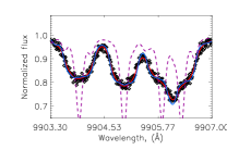
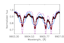
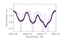
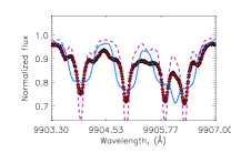
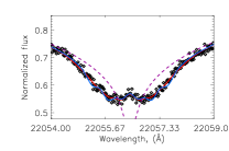
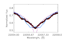
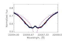
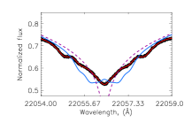
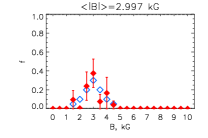
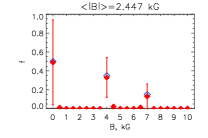
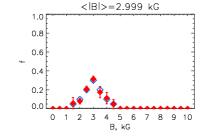
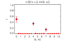
Figure 1: Forward simulation of FeH and Na i lines assuming two different distributions of surface magnetic fields. Thick black symbols – simulated observed spectrum; violet dashed line – computation with zero magnetic field; red line – computation with multi-component magnetic field shown on the bottom plots, blue line – computations with homogeneous magnetic field (i.e. $f=1$) of the same average intensity as multi-component magnetic field. Columns 1, 2 and 3, 4 correspond to the assumed SNR of $100$ and $500$ respectively. Atmospheric parameters are the same for all simulations. Blue open diamonds on the bottom plots show the true distribution of filling factors used to simulate observations.

In our investigation we employed the FeH line list of the Wing-Ford band ($F^{4}\,\Delta-X^{4}\,\Delta$ transitions) and molecular constants taken from Dulick et al. (2003). Transition probabilities for some of these lines were corrected according to Wende et al. (2010). Transition parameters for atomic lines were extracted from the VALD database (Piskunov et al. 1995; Kupka et al. 1999).

To compute synthetic spectra of atomic and molecular lines in the presence of a magnetic field, we employed the Synmast code (Kochukhov 2007). The code represents an improved version of the Synthmag code described by Piskunov (1999). It solves the polarized radiative transfer equation for a given model atmosphere, atomic and molecular line lists and magnetic field parameters. Model atmospheres are from MARCS the grid (Gustafsson et al. 2008).

In order to analyze the magnetic field via the spectral synthesis it is necessary to know the Landé g-factors of upper and lower levels of a particular transition. In case of atomic lines the necessary information was extracted directly from VALD. As shown by, e.g, Berdyugina & Solanki (2002) lines of FeH exhibit splitting that is in most cases intermediate between pure Hund’s case (a) and Hund’s case (b) and for which no analytic expression is possible. Therefore, to compute g-factors we implement an approach described in Shulyak et al. (2010) that is based on numerical libraries from the MZL (Molecular Zeeman Library) package originally written by B. Leroy (Leroy, 2004), and adopted by us for the particular case of FeH.

We attempt to measure the intensity and complexity of surface magnetic fields by carrying out a detailed synthetic spectral fitting. The lines of FeH are selected in such a way that their Zeeman patterns are accurately reproduced in the reference sunspot spectra for which both temperature and magnetic field are known independently from the fit to atomic lines, as shown in Shulyak et al. (2010). To fully characterize the magnetic field one needs to derive a) the surface averaged field modulus $\langle B_{\mathrm{s}}\rangle$ that affects the magnitude of the splitting between individual Zeeman components of a given line, and b) the geometry of the magnetic field that influences the intensity and shape of magnetically split lines. Note that a true and unique picture of the surface magnetic field can be restored by surface imaging techniques like Zeeman Doppler Imaging which relies on the rotationally modulated signals in polarized light or at least phase-resolved longitudinal magnetic field measurements with subsequent modelling of spectroscopic lines. Because only unpolarized Stokes $I$ spectra are available to us, however, it is impossible to draw conclusions about the geometry of the surface magnetic field in target stars. That is, no information about vector magnetic field and positions of magnetic areas on stellar surfaces can be derived. Nevertheless, even Stokes $I$ spectra alone contain information about the magnetic field structure or what we call the complexity of the magnetic field, i.e. the minimum number of magnetic field components required to fit the observed line profiles. The latter depend on the geometry of the magnetic field through the intensities of Zeeman $\pi$- and $\sigma^{\pm}$-components. This allows one to investigate how complex the magnetic field is compared to the case when it can be described by a single component having a fixed strength. For instance, a homogeneous magnetic field of a fixed strength and a configuration where the field is concentrated only in small surface areas (i.e. spots) would result in line profiles that look different. This can then be described in terms of magnetic filling factors ${f_{i}}$ which are nothing but a measure of the area on the stellar surface covered by a magnetic field of intensity ${|\mathrm{\mathbf{B}}|_{i}}$. In case of a homogeneous field ($f=1$) the mean surface magnetic field is $\langle B_{\mathrm{s}}\rangle=|\mathrm{\mathbf{B}}|$, while in case of more complex fields $\langle B_{\mathrm{s}}\rangle=\sum|\mathbf{B}_{i}|f_{i}$. The aim of the present work is to measure the distribution of filling factors by fitting theoretical and observed line profiles and to derive the minimum number of magnetic field components which provides an acceptable agreement between theory and observation. This approach is similar to those used by, e.g., Johns-Krull & Valenti (2000) with a difference of using many magnetically sensitive FeH lines instead of only a few atomic lines as well as accurate treatment of thousands of blends in the spectrum synthesis code.

The fitting procedure consists of the following steps. For each spectrum we apply a chi-square Levenberg-Marquardt minimization algorithm with filling factors $f_{i}$ as fit parameters. We consider $21$ filling factors which correspond to magnetic fields ranging from $0$ kG to $10$ kG in steps of $0.5$ kG. We sequentially start from $2$ filling factors and then add new ones one-by-one computing the corresponding $\chi^{2}$ and mean deviation $\sigma$ between observed and predicted spectra. The whole procedure is applied for different sets of atmospheric parameters: $T_{\rm eff}$, $\alpha(\mathrm{Fe})$, and $\upsilon\sin i$. We assume the same surface gravity, $\log(g)=5.0$, for all M-dwarfs. The effect of varying atmospheric parameters on the derived distributions of filling factors is also investigated. This is an important part of our work since little is known about the surface structure of active M-dwarfs: do they exhibit large cool or hot areas similar to sunspots and plage regions observed in the Sun? How is the magnetic field correlated with these regions, etc.? Measurements of stellar magnetic fields from spectroscopy requires that atmospheric parameters are accurately known, which is unfortunately not always the case because of well-known problems in matching spectra of M-dwarfs where errors in, e.g., effective temperatures and metallicities can be large. This raises another goal of our investigation, namely to see the impact of choosing different atmospheric parameters on the derived magnetic field and filling factors. Errors in atmospheric parameters are not the only uncertainties that affect the measurements of the magnetic fields. There are other potentially important effects like, e.g., temperature inhomogenities of active regions with bright and dark areas similar to those observed on the Sun which we ignore in the present study. A more in-depth analysis would be needed to fully account for complex morphologies of stellar photospheres. We plan to address these questions step-by-step in future calculations, assuming at present that the surface temperatures of sample stars are homogenous and can be accurately derived from magnetically insensitive lines.

The initial values of $T_{\rm eff}$ and $\upsilon\sin i$ for all targets were taken from RB07. The iron abundance was then adjusted to fit magnetically-insensitive FeH lines located at $\lambda\lambda 9914$ – $9916$, $\lambda\lambda 9925$ – $9928$, $\lambda 9945$, $\lambda 9957$, and $\lambda 9999$ regions. Because of the high densitiy of FeH lines, magnetically sensitive FeH lines are in most cases found in blends that contain many individual lines. In the present study the FeH features in the following spectral intervals have been used for the magnetic field measurements: $\lambda\lambda 9903.3-9907.0$, $\lambda\lambda 9908.3-9913.8$, $\lambda\lambda 9919.0-9921.6$, $\lambda\lambda 9928.0-9929.0$, $\lambda\lambda 9931.0-9933.5$, $\lambda\lambda 9938.5-9939.3$, $\lambda\lambda 9941.5-9942.6$, $\lambda\lambda 9945.5-9947.8$, $\lambda\lambda 9956.1-9958.80$, $\lambda 9961.3$. These intervals have been used in all calculations presented below and are same for all stars studed. As shown by 3D hydrodynamical simulations carried out by Wende et al. (2009), the velocity fields in atmospheres of M-dwarfs with temperatures $T_{\rm eff}<3500$ K are well below $1$ km/s. This has only weak impact on line profiles leaving Zeeman effect and rotation to be the dominating broadening mechanisms. Therefore we assumed zero micro- and macroturbulent velosities in all calculations.

To test whether our fitting method is capable of restoring the original solution under conditions when all atmospheric parameters are accurately known, we performed forward calculations of selected FeH and one Na i $\lambda 22056$ line using two distributions of filling factors: one with only three components of $0$ kG ($f=0.5$), $4$ kG ($f=0.35$), and $7$ kG ($f=0.15$), and another with seven components between $1.5$ kG and $4.5$ kG with a smooth Gaussian-like distribution of filling factors. The simulated “observed” spectra were computed for $T_{\rm eff}=3400$ K, $\upsilon\sin i=0$ km/s, and convolved with $R=100\,000$. We find that the code always finds a unique distribution of filling factors. However, because of implicit normalization requirement $\sum f_{i}=1$ the filling factors are highly correlated variables. Therefore, no meaningful estimate of error bars is possible based on the covariance matrix provided by the minimization technique. Instead, we provide estimates of a significance of every magnetic field component. For each magnetic field distribution the following procedure is applied:

1. Noise is added to the simulated spectra. The noise amplitude ($1\sigma$) ranges from 2% to 0.001% which covers the SNR of spectra of target stars in our sample.

2. For each simulated spectrum with a given noise level a distribution of magnetic fields and their filling factors are derived. The spectra computed from these distributions of filling factors are then taken as a reference to compute the significance for each magnetic field component.

3. For each magnetic field component $f_{i}>0$ its filling factor is decreased by a chosen amount $\Delta f$. At the same time, the filling factor of the field component left of it (e.g., $f_{i-1}$) is increased by the same amount so that the condition $\sum f_{i}=1$ always holds.

4. The adjusted distribution of filling factors obtained at the previous step is then used to compute a synthetic spectrum and its deviation from the reference spectrum computed with best fit distribution in step 2.

5. The adjustment of a given filling factor is repeated until the maximum deviation from the reference spectrum at any fit point is larger than the $1\sigma$ error which was used to generate the simulated spectrum on step 1.

The described procedure allows us to estimate a significance of a particular magnetic field component relative to its closest neighbor and to verify whether there is another solution possible within a specified SNR of the simulated observations. For the sake of consistency we will call these significane intervals error bars, though one should remember that they do not represent statistical error bars provided by the minimization procedure. Despite its simplicity, the proposed method provides information about the uniqueness of solutions for filling factors and thus gives a robust overview of field distributions in individual stars. It also has an advantage of reducing computation time considereably compared to, e.g., direct Monte-Carlo simulations which are preferred but currently very challenging to run because of complex spectra of FeH lines.

It is clear that the solution and corresponding error bars are strongly dependent upon SNR of observations. As an example, Fig. 1 shows results of two simulations with different distributions of filling factors and SNR values of $100$ and $500$. The simulations were done assuming the magnetic field model with a dominating radial field component (see below). Two main conclusions can be drawn. First, the lowest SNR needed to restore the shape of the filling factors distribution is SNR$>300$ and the original amplitudes are restored with SNR$\approx 500$, as shown in the last two columns of Fig. 1. With SNR$=100$ it is challenging to restore a complex distribution of magnetic fields similar to that shown on, e.g., lower left plots of Fig. 1 where many components are localized in a particular range of field strength. However, distributions where only a few field components are present and well separated from each other are accurately reconstructed, although their significance is small. In other words, the lower plot on the second column of Fig. 1 shows that, e.g., the component of $7$ kG strength can be replaced by a component with a $6.5$ kG strength and still provide a similar quality of the fit to the line profiles within the error bars of the observations. The only difference is that the $7$ kG component provides a smaller deviation between the observed and synthetic spectra. A second thing to note is that the restored mean magnetic field $\langle B_{\mathrm{s}}\rangle=\sum|\mathbf{B}_{i}|f_{i}$ is always equal to the original value even if the reconstructed amplitudes of filling factors deviate.

Because only unpolarized Stokes $I$ spectra are analyzed in this paper, no information about vector magnetic field could be retrieved. Therefore, we made use of a simple magnetic field model described with a small number of free parameters. The field is homogeneous in the stellar reference frame and is specified by the three vector components: radial $B_{\rm r}$, meridional $B_{\rm m}$, and azimuthal $B_{\rm a}$, reckoned in the spherical coordinate system whose polar axis coincides with the line of sight. Then, the two field components relevant for calculating the Stokes $I$ profiles are given by

$$B_{\rm l}=B_{\rm r}\cos{\theta}-B_{\rm a}\sin{\theta}$$ (1)

for the line of sight component and

$$B_{\rm t}=\left[(B_{\rm r}\sin{\theta}+B_{\rm a}\cos{\theta})^{2}+B_{\rm m}^{2}\right]^{1/2}$$ (2)

for the transverse component. In practice it is sufficient to adjust $B_{\rm r}$ and $B_{\rm m}$, keeping $B_{\rm a}$ zero.

This approximation of the magnetic field structure is undoubtedly simplistic and unsuitable for describing phase-dependent four Stokes-parameter profiles of magnetic M dwarfs. Nevertheless, as shown by the previous studies of Zeeman-sensitive lines in cool stars (Johns-Krull & Valenti 1996; Johns-Krull 2007), it is sufficient for modelling unpolarized spectra of M dwarfs and T Tauri stars with strong fields.

In the following we assume that the stellar surface is covered by a dominating radial (RC model hereafter, $B_{\rm m}=B_{\rm a}=0$) or meridional (MC model hereafter, $B_{\rm r}=B_{\rm a}=0$) field component and perform respective calculations for each target star.

4 Testing molecular and atomic diagnostics

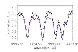
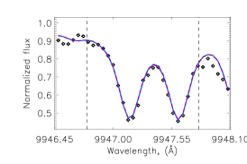
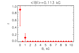
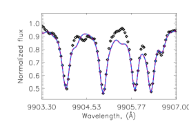
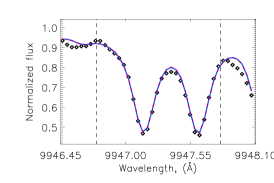
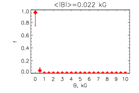
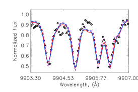
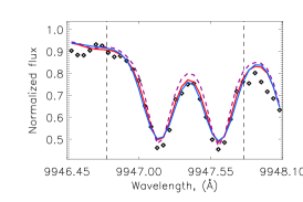
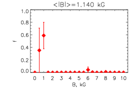
Figure 2: Examples of theoretical fit to selected FeH lines and resulting distributions of filling factors for two spectra of GJ 1002 taken in two different observing runs with CRIRES. Top panel – run 385.D-0273, $T_{\rm eff}=3100$ K, $\alpha(\mathrm{Fe})=-4.37$, $\upsilon\sin i=2.43$ km/s. Middle panel –  run 079.D-0357, $T_{\rm eff}=3100$ K, $\upsilon\sin i=1.85$ km/s, $\alpha(\mathrm{Fe})=-4.47$. Bottom panel – same as top panel but adopting atmospheric parameters from middle panel: implementation of these parameters results in a spurious detection of the magnetic field as illustrated on the corresponding plot of filling factors (see text). Violet dashed line – computation with zero magnetic field, red line – computation with multi-component magnetic field shown on the right hand side, blue line – computations with homogeneous magnetic field (i.e. $f=1$) of the same average intensity as multi-component magnetic field. Vertical dashed lines mark the edges of the actual fit region.

Our observations cover the range of FeH lines at $1$ $\mu$m and strong Na i lines at $2.2$ $\mu$m. Presumably, the magnetic fields derived independently from these two sets of lines must agree, if the atmospheric model structure and/or physical conditions in the line formation depths are accurately predicted by model atmospheres and spectrum synthesis codes. Sadly, we find this is not always the case: one needs noticeably different temperatures to fit FeH and Na lines. In particular, wide wings of the later demand a lower $T_{\rm eff}$ compared to FeH lines. As a result, magnetic fields derived from best-fit spectra assuming fixed $T_{\rm eff}$ deviate from one another. A good illustration can be seen from the analysis of a non-magnetic M$4.5$ dwarf GJ 1002. This star shows no detectable X-ray emission and thus the corresponding surface magnetic field of the star is expected to be nearly zero or absent. The atmospheric parameters were derived from the fit to magnetically insensitive FeH lines and are consistent with estimates from previous independent studies: $T_{\rm eff}=3100$ K, $\alpha(\mathrm{Fe})=-4.37$, $\upsilon\sin i=2.4$ km/s. For instance, Shulyak et al. (2010) used $T_{\rm eff}=3100$ K, $\alpha(\mathrm{Fe})=-4.37$, $\upsilon\sin i=2.5$ km/s. Note that values of $\alpha(\mathrm{Fe})$ and $\upsilon\sin i$ depend strongly on the effective temperature adopted, but also on the continuum normalization and data quality. For instance using the same spectra from Shulyak et al. (2010) but a slightly different continuum normalization procedure yields $\upsilon\sin i=1.85$ km/s, $\alpha(\mathrm{Fe})=-4.47$. The magnetic field derived from the former set of parameters is only about $100$ G (which we consider as no detection within observed error bars, because such a small field causes very insignificant changes in theoretical line profiles compared to precise zero field calculation), while it is zero if the later set of parameters was used.

Examples of theoretical fits to a few FeH lines assuming the RC model of the magnetic field and resulting distributions of filling factors are illustrated on the first two panels of Fig. 2. The error bars for the filling factors were computed as described in the previous section. Note that different combinations of atmospheric parameters are allowed as long as they fit the observed magnetically insensitive lines. For instance, one of the unknown parameters in fitting FeH lines is the constant of van der Waals broadening $\gamma_{\mathrm{Waals}}$. It was shown in Shulyak et al. (2010) that, in order to fit FeH lines in GJ 1002 with a given $T_{\rm eff}=3100$ K and $\upsilon\sin i=2.5$ km/s, the value of $\gamma_{\mathrm{Waals}}$ must be increased by an enhancement factor of $f(\gamma_{\mathrm{Waals}})=3.5$ compared to a classical value given in Gray, (1992). Note that different combinations of atmospheric parameters such as iron abundance, $\gamma_{\mathrm{Waals}}$, and $\upsilon\sin i$ could provide the same accurate fit to the observed spectra: a change in one of these parameter could be compensated (to a certain extent) by an opposite change in the others. For example, decreasing $f(\gamma_{\mathrm{Waals}})=1.75$ would require $\alpha(\mathrm{Fe})=4.30$, $\upsilon\sin i\approx 2.0$ for the spectra of GJ 1002 from our run 385.D-0273. The bottom line of this example is that small inaccuracies in atmospheric parameters, although they might be small when comparing theoretical fits to individual lines, might result in a spurious detection of magnetic fields, in particular for multi-component solutions. An illustrative example is shown in the bottom panel of Fig. 2 where we apply atmospheric parameters derived from the spectra of the two CRIRES runs. In both these cases we detect nearly zero magnetic fields ($0.113$ kG and $0.022$ kG respectively) as long as we apply individual atmospheric parameters derived from the fit to the magnetic insensitive lines in the spectra of each run, but detect a spurious $\langle B_{\mathrm{s}}\rangle=1.14$ kG field when applying atmospheric parameters from one run to fit the spectrum of another. This is a purely numerical artifact because in this particular case the fitting algorithm increases the Zeeman broadening to compensate for the corresponding differences in $\upsilon\sin i$ and $\alpha(\mathrm{Fe})$ between the runs. Ideally the atmospheric parameters derived from the two spectra of the same star must be the same. In reality, however, this is not the case mainly because of differences in SNR and continuum normalization that affect depths of spectroscopic features. This exercise highlights the importance of using magnetically insensitive lines for the determination of atmospheric parameters that might need to be adjusted once new data, improved line lists, model atmospheres, etc. are being used. Following this procedure helps to avoid false detections of magnetic fields.

The main problem in using a multi-component approach for the magnetic field measurements is its sensitivity to the line shapes that are largely affected by data processing algorithms and inaccuracies in atomic/molecular parameters. In the case of FeH lines, no individual Zeeman components can be seen because of the large number of individual $\pi$ and $\sigma^{\pm}$ components relevant for every single transition, which are smeared out and result only in line broadening. This is not the case for all FeH lines as will be described below, but is true for smaller fields when Zeeman components of nearby strong lines do not overlap. Such broadening can easily be mimicked by an appropriate choice of the rotational velocity. This degeneracy can be removed by the use of magnetically insensitive lines.

The spectrum of GJ 1002 observed with CRIRES in run 079.D-0357 also contains strong Ti i lines in the $\lambda\lambda 10\,300-10\,700$ region. We used less blended lines at $\lambda 10399$, $\lambda 10498$, and $\lambda 10587$ to test our method when applied to atomic transitions. Unfortunately, all sets of atmospheric parameters derived from FeH lines are consistent with non-zero magnetic fields. Adjusting $\alpha(\mathrm{Ti})$ for a fixed $T_{\rm eff}=3100$ K does not help to solve the problem of fitting the wings of Ti lines which we find to be the main reason for the detection of non-zero magnetic field. The top panel of Fig. 3 shows a fit to Ti lines with $T_{\rm eff}=3100$ K, $\upsilon\sin i=2.4$ km/s, $\alpha(\mathrm{Ti})=-7.24$. A $\upsilon\sin i=1.9$ km/s (adopted from FeH lines) results in too deep line cores, but almost in the same strength of the magnetic field detected (middle panel of Fig. 3). In order to obtain a nearly zero magnetic field one has to decrease the effective temperature to $T_{\rm eff}\approx 3050$ K and increase rotational velocity to $\upsilon\sin i\approx 2.6$ km/s, as shown on the bottom panel of Fig. 3. It is seen that in the latter case magnetic field components as strong as $10$ kG appear, but this is obviously an artifact of the method: such a high component occasionally provides a better fit to line wings though its impact on the line profiles is very small. A non-detection of the magnetic field is obtained assuming $\upsilon\sin i=3$ km/s, and the example of using $\upsilon\sin i=2.6$ km/s shows that the highest field components may easily result from uncertainties in rotational velocities and instrument resolving power. Finally note that the tested Ti lines are not very magnetic sensitive, with effective Landé factors $g_{\rm eff}\approx 1$, therefore strong fields are needed to mimic small adjustments in $\upsilon\sin i$ described above.

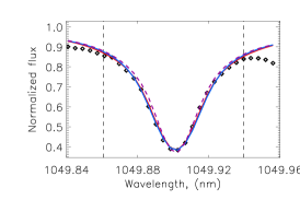
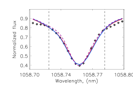
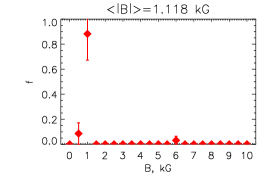
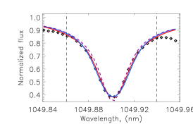
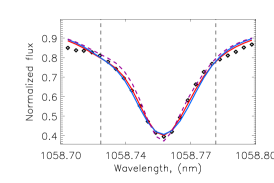
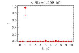
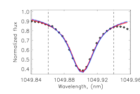
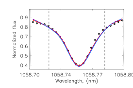
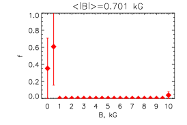
Figure 3: Same as on Fig. 2 but for Ti i in GJ 1002. Top panel – $T_{\rm eff}=3100$ K, $\alpha(\mathrm{Ti})=-7.24$, $\upsilon\sin i=2.43$ km/s. Middle panel – $T_{\rm eff}=3100$ K, $\alpha(\mathrm{Ti})=-7.24$, $\upsilon\sin i=1.85$ km/s. Bottom panel – $T_{\rm eff}=3050$ K, $\alpha(\mathrm{Ti})=-7.24$, $\upsilon\sin i=2.60$ km/s.

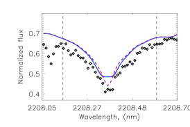
Figure 4: Same as on Fig. 3 but for Na i lines. Atmospheric parameters are: $T_{\rm eff}=3100$ K, $\alpha(\mathrm{Na})=-5.87$, $\upsilon\sin i=2.43$ km/s.

No set of atmospheric parameters adopted from the above investigation provide a reasonable fit to Na i lines at $2.2$ $\mu$m. These lines appear to be too wide and their profiles are strongly affected by stellar water lines to allow for an accurate analysis. That is, there is always an unknown vertical offset if one attempts to synthesize those lines. To improve the quality of the theoretical fit we used a list of water lines to determine the continuum offset and then shift each observed spectrum accordingly in such a way that quasi-continuum levels in both observed and theoretical spectra match. The list of water lines is taken from R. Kurucz’ website. Still, this does not solve the problem completely, most probably because of intrinsic inaccuracies of the water list itself.

Figure 4 illustrates the problem. Even shifting each line vertically in the attempt to account for the unknown continuum level would not help to achieve a zero magnetic field detection because lines remain too wide still. Note that depths and widths of Na lines (as well as Ti lines) are well fit in the spectrum of the solar photosphere, and thus the problem that we encounter for these lines in cool M-dwarf spectra does not arise from possibly inaccurate line transition parameters. Therefore we decided not to use Na lines for the magnetic field measurements. This is a disappointing result because Na lines are strong features that probe a wide range of atmospheric depths. However, they can be used only when accurate telluric modelling, improved molecular line lists, and more accurate continuum normalization methods will become available.

5 Results

In this section we present results of magnetic field determination for individual M-dwarfs, which are also combined altogether in Table 2. As follows from the previous section, the Na i lines can not be used for field measurements and the region of the Ti i lines (though they appear to be good indicators of atmospheric structure) was not covered by our observational settings. Therefore the results presented in this section are from FeH lines alone.

5.1 GJ 388 (AD Leo)

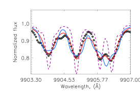
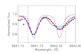
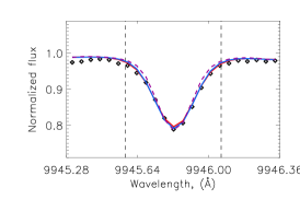
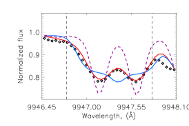
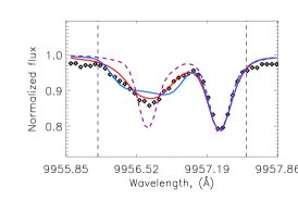
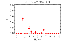
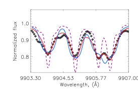
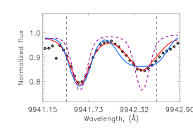
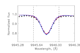
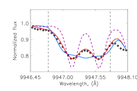
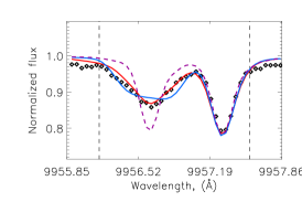
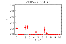
Figure 5: Examples of theoretical fit to selected FeH lines and resulting distributions of filling factors for GJ 388 assuming RC (first and second raws) and MC (third and forth rows) magnetic field models. Atmospheric parameters $T_{\rm eff}=3400$ K, $\alpha(\mathrm{Fe})=-4.64$, $\upsilon\sin i=3$ km/s. Violet dashed line – computation with zero magnetic field, red line – computation with multi-component magnetic field shown on the right bottom plot, blue line – computations with homogeneous magnetic field (i.e. $f=1$) of the same intensity as multi-component magnetic field.

GJ 388 is an M$3.5$ star with a rotational velocity of $\upsilon\sin i\leqslant 3$ km/s  $T_{\rm eff}=3400$ K, and surface magnetic field of $2.9$ kG as estimated in RB07.

From magnetically insensitive FeH lines we estimated the iron abundance to be $\alpha(\mathrm{Fe})=-4.64$. We find that $\upsilon\sin i$ does not influence the determination of the magnetic field if decreased below $3$ km/s: it can always be compensated by the respective increase of the iron abundance to obtain a similar quality of the fit. The derived mean magnetic field strength matches the value given by RB07, that is $\langle B_{\mathrm{s}}\rangle=2.9$ kG.

Figure 5 illustrates the comparison between observed and predicted profiles of some FeH lines. It reveals the strong sensitivity of FeH features to the magnetic field configuration, i.e. to the presence of different magnetic field components. FeH lines at $\lambda 9906$ and $\lambda 9947$ are the most illustrative examples of Zeeman broadening, (but see also lines at $\lambda 9942$ and $\lambda 9956$).

The distribution of the magnetic field that we recover depends critically upon the assumed magnetic field model used in spectrum synthesis. Employing the RC model results in one strong component of $1.5$ kG covering about $50$% of the visible stellar surface. There are four other significant field components covering the rest of the surface with intensities spread between $3$ kG and $6.5$ kG. These components appear from the necessity to obtain a match between the narrow cores (requiring weak field components) and wide wings (requiring strong field components). There is no significant zero field component, and we do not find any zero-field component when we applied different atmospheric parameters. For instance, using a higher temperature of $T_{\rm eff}=3500$ K, $\upsilon\sin i=3$ km/s, and solar $\alpha(\mathrm{Fe})=-4.54$ results in a similar distribution of filling factors as well as $\langle B_{\mathrm{s}}\rangle$ value. A zero-field component appears when the MC model is assumed. In addition, the components of $2$ kG and $2.5$ kG of the same filling factors ($f\approx 0.25$) appear. The strongest $6.5$ kG component stays similar to that found in the case of RC model. The detection of a zero-field component is not surprising because Zeeman $\pi$-components are deep in MC model compared to RC one, therefore they immediately provide a good fit to sharp line cores of such features as, e.g., $\lambda 9942$ and $\lambda 9956$.

Although the two magnetic field models result in distributions of filling factors that look different, we always find at least three distinct groups of magnetic field components and no smooth distributions are ever detected. The derived mean magnetic fields $\langle B_{\mathrm{s}}\rangle$ are very similar too. By examining individual lines we find that the MC model provides, on average, a better fit to observations.

5.2 GJ 729

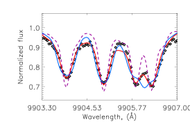
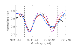
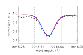
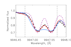
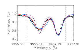
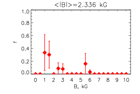
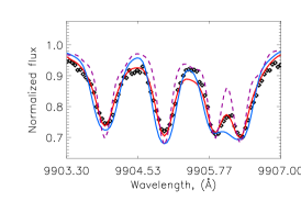
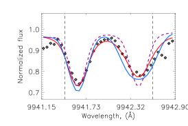
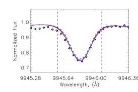
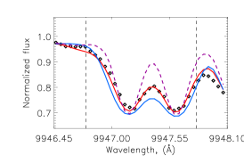
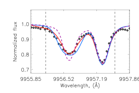
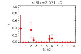
Figure 6: Same as on Fig. 5 but for GJ 729. Atmospheric parameters $T_{\rm eff}=3400$ K, $\alpha(\mathrm{Fe})=-4.40$, $\upsilon\sin i=4$ km/s.

GJ 729 is classified as M$3.5$ star for which RB07 provide $\upsilon\sin i\approx 4$ km/s and $\langle B_{\mathrm{s}}\rangle=2.2$ kG. The best fit between theory and observations was obtained employing atmospheric parameters from RB07 and $\alpha(\mathrm{Fe})=-4.40$. Assuming solar iron abundance $\alpha(\mathrm{Fe})=-4.54$ results in a lower effective temperature of $T_{\rm eff}=3300$ K in order to obtain the same quality of the fit. The distributions of filling factors look very similar for these two sets of atmospheric parameters. Because the first set provides formally a better fit, we prefer it to the latter. Figure 6 illustrates the match between theory and observations. The magnetic field of the star appears to be distributed over three groups of components. For the RC model we find components with the small $1-1.5$ kG, moderate $2.5-3$ kG, and strong $5.5$ kG intensities. Although errors bars are large, the existence of such distinct features as FeH $\lambda 9906$ demonstrate that well-separated deep cores only appear with $2.5-3$ kG magnetic field components so that their significance is well constrained. A similar three-like component distribution is also recovered when assuming MC model, but as in the previous case of the GJ 388, a strong zero-field component appears ($f=0.4$) along with a $2$ kG component of the similar strength. The mean magnetic fields are also a bit different and amount to $\langle B_{\mathrm{s}}\rangle=2.3$ kG and $\langle B_{\mathrm{s}}\rangle=2.1$ kG respectively. Finally, we do not prefer either of the two cases by looking at individual line profiles.

5.3 GJ 285 (YZ CMi)

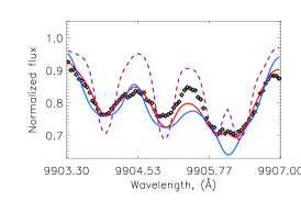
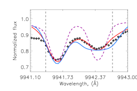
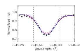
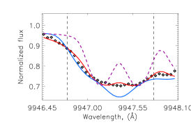
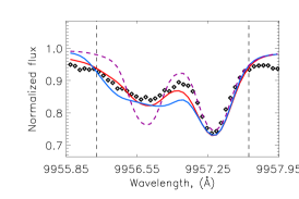
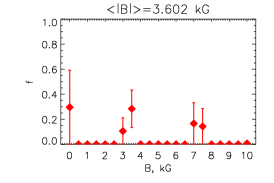
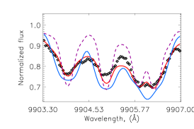
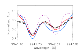
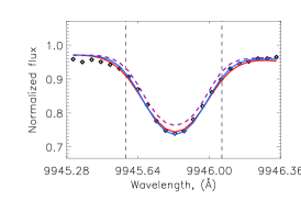
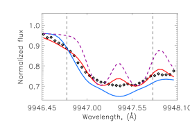
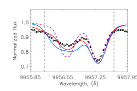
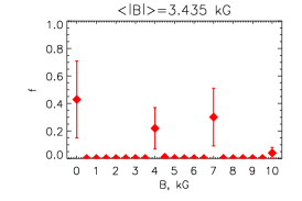
Figure 7: Same as on Fig. 5 but for GJ 285. Atmospheric parameters $T_{\rm eff}=3300$ K, $\alpha(\mathrm{Fe})=-4.37$, $\upsilon\sin i=6$ km/s.

GJ 285 is another very active M$4.5$ dwarf with rotational velocity of about $\upsilon\sin i\approx 5$ km/s. RB07 derived a lower limit for the mean surface magnetic field of $\approx 3.9$ kG. We find a stable solution for filling factors using an enhanced iron abundance and a faster rotation velocity of $\upsilon\sin i=6$ km/s, as illustrated in Fig. 7. The RC model reveals five significant magnetic field components: one zero field, two components with $3$ kG and $3.5$ kG field, and two with very strong $7$ kG and $7.5$ kG fields. They give in total a mean magnetic field of $\langle B_{\mathrm{s}}\rangle=3.6$ kG, which is $0.3$ kG lower then reported in RB07. Employing $\upsilon\sin i=5$ km/s results in $\langle B_{\mathrm{s}}\rangle=3.9$ kG, but this increase in $\langle B_{\mathrm{s}}\rangle$ is then caused by the appearance of a non-zero $10$ kG field component which (as we argued for the case of GJ 1002) is likely spurious because it lowers $\chi^{2}$ by a better match to the far wings only. Using $\upsilon\sin i=6$ km/s provides the best overall fit between observed and predicted spectra. The MC model gives a very similar distribution of filling factors with a zero-field, $4$ kG, and $7$ kG components. But the resulting mean magnetic field is then $0.2$ kG lower compared to RC model, i.e. $\langle B_{\mathrm{s}}\rangle=3.4$ kG. From Fig. 7 one can see that the fit to FeH lines is not always accurate. Lines like $\lambda 9905$ are possibly affected by data reduction issues because they are fit accurately in spectra of, e.g., GJ 388. Next, the observed line at $\lambda 9947$ does not seem to show a doubled profile but the synthetic spectra predicts one. This may tell us that the intensity of the magnetic field could be even lower than what we have found here. From the comparison of line profiles it is clear that the RC model provide a better fit to observations. Lines like FeH $\lambda 9942$, and $\lambda 9956$ are obviously too strong and the central feature of $\lambda 9947$ is not reproduced when using the MC model.

5.4 GJ 406 (CN Leo)

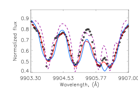
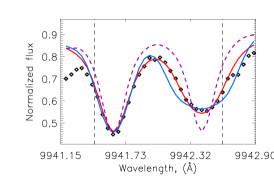
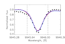
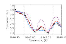
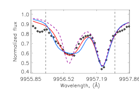
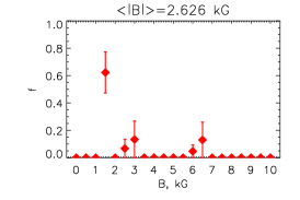
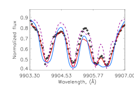
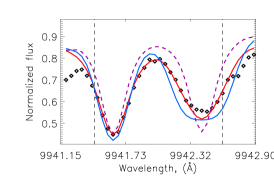
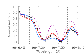
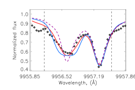
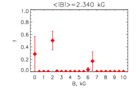
Figure 8: Same as on Fig. 5 but for GJ 406. Atmospheric parameters $T_{\rm eff}=3100$ K, $\alpha(\mathrm{Fe})=-4.08$, $\upsilon\sin i=3$ km/s.

GJ 406 is a coolest target we analyze in this paper. It is of spectral type M$5.5$ and a slow rotator with $\upsilon\sin i=3$ km/s (RB07). We find the best fit atmospheric parameters $T_{\rm eff}=3100$ K, $\alpha(\mathrm{Fe})=-4.08$, $\upsilon\sin i=3$ km/s. Using a solar iron abundance we were not able to obtain an accurate fit FeH lines such as $\lambda 9942$, $\lambda 9950$, and $\lambda 9956$ while matching profiles of all other FeH lines. Moreover, the solar iron abundance systematically led to a much lower $T_{\rm eff}=2900$ K which is inconsistent with the assigned spectral type of the star. Therefore we preferred a model with $T_{\rm eff}=3100$ K thought with a high iron abundance of $\alpha(\mathrm{Fe})=-4.08$. Figure 8 demonstrates the fit to the FeH lines and the distribution of filling factors. The latter reveals a strong $1.5$ kG component with $f=0.6$, two components with of $2.5$ kG and $3$ kG, and two components of $6$ kG and $6.5$ kG strength when employing RC model. The mean magnetic field strength is $\langle B_{\mathrm{s}}\rangle=2.6$ kG. The MC model leads to a $f=0.3$ zero-field component and strong $f=0.55$ component of $2$ kG, as well as weak $f=0.2$ component of $6.5$ kG. This model gives a mean $\langle B_{\mathrm{s}}\rangle=2.3$ kG, i.e. $\approx 0.3$ kG lower compared RC case.

Table 2: Magnetic field measurements in M-dwarfs.

Name	$T_{\rm eff}$	$\alpha(\mathrm{Fe})$	$\upsilon\sin i$	$\langle B_{\mathrm{s}}\rangle^{a}$		$\sigma^{b}$		$Bf$ (RB07)c	$B_{max}$d
	K	dex	km/s	kG		%		kG	kG
				RC	MC	RC	MC
GJ 388	$3500$	$-4.46$	$2.9$	$2.8$	$2.9$	$1.69$	$1.92$	$2.9\pm 0.2$	$7.0$
	$3400$	$-4.64$	$3.0$	$2.9$	$2.9$	$1.48$	$1.53$		$6.5$
	$3300$	$-4.73$	$2.7$	$2.7$	$2.8$	$1.64$	$1.81$		$7.0$
GJ 729	$3500$	$-4.30$	$4.4$	$2.4$	$2.3$	$1.72$	$1.68$	$2.2\pm 0.1$	$5.5$
	$3400$	$-4.40$	$4.0$	$2.3$	$2.1$	$1.66$	$1.74$		$6.0$
	$3300$	$-4.54$	$4.0$	$2.2$	$1.9$	$1.67$	$1.75$		$6.0$
GJ 285	$3400$	$-4.22$	$6.2$	$3.6$	$3.4$	$2.03$	$2.11$	$>3.9$	$7.5$
	$3300$	$-4.37$	$6.0$	$3.6$	$3.4$	$2.00$	$2.10$		$7.5$
	$3200$	$-4.57$	$6.2$	$3.5$	$3.6$	$1.95$	$1.97$		$7.0$
GJ 406	$3200$	$-3.80$	$3.0$	$2.3$	$2.0$	$4.03$	$4.36$	$2.4\pm 0.1$	$7.0$
	$3100$	$-4.08$	$3.0$	$2.6$	$2.3$	$3.94$	$3.87$		$6.5$
	$3000$	$-4.26$	$1.0$	$2.2$	$2.0$	$4.10$	$4.36$		$6.5$
GJ 1002	$3100$	$-4.37$	$2.4$	$<$0.1		$1.05$		$0.0$	$1.0$
	$3100$	$-4.47$	$1.9$	$<$0.02		$0.98$			$0.5$

^a – mean magnetic field derived assuming magnetic field models with dominating radial (RC) and meridional (MC) components
^b – deviation between observed and predicted profiles of FeH lines computed using Eqn. (3)
^c – values are from Reiners & Basri (2007)
^d – strength of the maximum field component detected

6 Discussion

6.1 Indicators of Zeeman splitting

While most previous studies were based on only a few (or one) atomic lines at visual wavelengths, in this work we attempted to extend the spectroscopic investigation of magnetic fields in M-dwarfs by using numerous lines of the FeH molecule. We used CRIRES@VLT to obtain high resolution $R=100\,000$ spectra of four well known M-dwarfs in the FeH Wing-Ford band and Na i lines in the K-band. Our goal was to measure the complexity of the magnetic fields in these stars by using direct spectrum synthesis and up-to-date models of Zeeman splitting of FeH lines developed and tested in Shulyak et al. (2010). What we mean here by “complexity” of the field is the minimum number of filling factors (each corresponding to a given magnetic field intensity) required to fit the observed line profiles for a given set of atmospheric parameters. The distribution and amplitude of filling factors contain information about the possible structure of surface magnetic fields.

As shown by our forward simulations, the restored distribution of filling factors depends critically on the SNR of the observed spectrum. If the SNR is of the order of $100$ the derived amplitude of filling factors may be biased if the real distribution is smooth, i.e., similar to those presented in the lower left plot of Fig. 1. On the other hand, the value of the average surface magnetic field can be reproduced in all cases. In our sample, GJ 285 and GJ 388 have SNR $>200$, while GJ 729 and GJ 406 have SNR $100-130$. Because the shape of the magnetic field distribution is less affected by SNR we do not expect strong changes in the corresponding results if higher SNR observations were available, but we note that comprehensive analysis is possible only with SNR$>300$.

We confirm that FeH lines are suitable indicators of magnetic fields as they contain both magnetically very sensitive and magnetically insensitive lines in a $\approx$100 Å window of the Wing-Ford band. Additionally, there are very few lines of other species in that region except FeH, only some very weak atomic lines, i.e. FeH lines do not suffer blends of other species. Lines at $\lambda\lambda 9903-9907$ and $\lambda 9947$ are also excellent diagnostics of the complexity of the magnetic field because of the characteristic behaviour of their line shapes as a function of the field distribution.

On the other hand, we failed to fit lines of Na i even in a presumably non-magnetic reference star GJ 1002. Since this spectral region is known to be crowded by numerous stellar water lines it is likely that we failed to perform an appropriate continuum normalization of the spectra. Unfortunately, CRIRES only provides data in very narrow wavelengths intervals, about $\Delta\lambda\approx 100$ Å in that region, which makes a reliable continuum determination very difficult.

As additional check for the consistency between atomic and FeH spectra, we used strong Ti i lines at $1.1$$\mu$m. Some of these lines are wide features with weak or no detectable blending. In the case where our method detects no or an insignificant magnetic field from FeH lines, it resulted in a detection when only Ti lines were used. This is because of a mismatch between observed and predicted profiles in the wings of the Ti lines. In order to obtain a solution that is consistent with a field-free situation we had to decrease $T_{\rm eff}$ of the star by $50$ K and slightly increase $\upsilon\sin i$. Obviously, we do not expect FeH and Ti lines to form under such different physical conditions: the atmosphere of the star should be homogeneous, in particular in absence of substantial magnetic activity. The difference may partly be explained by atomic and molecular lines being formed at different atmospheric layers, but it is more likely a sign of some missed physics, e.g., van der Waals broadening of Ti lines at such cool temperatures that differs from the classical treatment that we use in our spectral synthesis.

6.2 Comparison to earlier field measurements

We summarize our magnetic field measurements in Table 2. For each star, we provide the three best-fit solutions, one for our best estimate of $T_{\rm eff}$, and in addition, two solutions assuming a $\pm 100$ K uncertainity on $T_{\rm eff}$, which corresponds to roughly $0.5$ stellar spectral types. With this assumption, $\alpha(\mathrm{Fe})$ and $\upsilon\sin i$ were determined by least-square fitting to the magnetically insensitive FeH features listed in Sect. 3 before the magnetic field distribution was calculated including all available spectral features. We note that in most cases the simultaneous least-square fit to all atmospheric parameters did not yield a statistically meaningful solution (the formal reduced $\chi^{2}$ was always much larger than $1$), which results in underestimation of uncertainties, in particular in the average magnetic field. Therefore, we do not provide formal uncertainties from $\chi^{2}$ intervals but calculate the effect of varying atmospheric parameters, which is the dominating source of error. The difference between the mean magnetic fields for the three solution in $T_{\rm eff}$ are shown in Table 2, and they can be used as a measure of the uncertainity of the magnetic field measurements. In addition, columns 5 and 6 of the Table 2 contain values of the cumulative deviation between observed and predicted line profiles computed as following:

$$\sigma=\displaystyle\sqrt{\displaystyle\frac{1}{N}\sum_{i}^{N}\left(f_{i}^{\rm obs}-f_{i}^{\rm pred}\right)^{2}}.$$ (3)

The last two rows of Table 2 list the two sets of atmospheric parameters of GJ 1002 discussed in Sect. 3.

It is interesting to compare our results to measurements of magnetic fields in the literature. First, Saar & Linsky (1985) used five Ti lines in the K-band to measure the magnetic field of GJ 388. They found an average $|\mathrm{\mathbf{B}}|=3.8$ kG and $f=0.73$ so that $(|\mathrm{\mathbf{B}}|f)=2.8$ kG. Later, Johns-Krull & Valenti (2000) employed a method similar to the one we used to a few atomic lines finding $\sum|\mathbf{B}_{i}|f_{i}=3.3$ kG. This is very close to $\sum|\mathbf{B}_{i}|f_{i}=3.2$ kG derived by Kochukhov et al. (2009). Using the results from Johns-Krull & Valenti (1996), RB07 report a value of $\langle B_{\mathrm{s}}\rangle=2.9$ kG, which is identical to the value we derive here from FeH lines, independent upon the magnetic field model used.

For GJ 729 Johns-Krull & Valenti (2000) found $\sum|\mathbf{B}_{i}|f_{i}=2.0$ kG, the corresponding value from RB07 is $\langle B_{\mathrm{s}}\rangle=2.2$ kG, again in a good agreement with what we find: $\langle B_{\mathrm{s}}\rangle=2.3$ kG and $\langle B_{\mathrm{s}}\rangle=2.1$ kG employing RC and MC models respectively (recall that the average surface magnetic field $\langle B_{\mathrm{s}}\rangle=\sum|\mathbf{B}_{i}|f_{i}$, where $\langle B_{\mathrm{s}}\rangle_{i}$ runs from $0$ kG to $10$ kG).

Next, for GJ 285 Johns-Krull & Valenti (2000) reported $\sum|\mathbf{B}_{i}|f_{i}=3.3$ kG, which is much smaller then the lower limit of $\langle B_{\mathrm{s}}\rangle>3.9$ kG given by RB07. A recent study by Kochukhov et al. (2009) provides $\sum|\mathbf{B}_{i}|f_{i}=4.5$ kG. Our estimates are $\langle B_{\mathrm{s}}\rangle=3.6$ kG and $\langle B_{\mathrm{s}}\rangle=3.4$ kG for the RC and MC models, respectively, which fall between the earlier measurements.

For the coolest star in our sample, GJ 406, Reiners et al. (2007) found $\langle B_{\mathrm{s}}\rangle=2.2$ kG in a campaign spanning three observing nights. Intra-night magnetic variability was found to be significant at the level of $100$ G. We find $\langle B_{\mathrm{s}}\rangle=2.6$ kG and $\langle B_{\mathrm{s}}\rangle=2.3$ kG employing RC and MC models while RB07 derived a value of $\langle B_{\mathrm{s}}\rangle=2.4$ kG.

Thus, in general, measurements taken at different times are in good agreement considering the substantial uncertainties reported by all authors and the different spectral indicators used. Nevertheless, it is interesting to note that the highest variability (both absolute and relative) occurs in the most active star GJ 285 which has the strongest mean surface magnetic field and the highest level of x-ray luminosity among other stars in our sample (Schmitt & Liefke 2004). To what extent this reflects the variability of the magnetic fields or differences between measurement techniques remains to be identified.

6.3 Field distributions

For our sample stars, we have determined distributions of magnetic fields rather than average values alone. A great advantage of our method is that it is able to capture the full magnetic field distribution on the surface of a star regardless of the field polarity and geometry. All four stars show distinct groups of different magnetic field strength. We did not find solutions with homogeneous field distributions ($f=1$ for the component that equals the average field), and we did not find solutions in which different field strengths are equally represented on the stellar surfaces ($f=const.$ for all values of $B$ up to $B_{\rm max}$). This is an interesting result because the average fields on the four stars are on the order of the maximum field strength we observe in sunspots. This implies that large surface regions contain fields that are always on the order of those in small scale sunspots. Magnetic field saturation (see Reiners et al. 2009) would then occur because the entire stellar surface is populated with a field strength on the order of 2–3 kG, while the local field strength does not change. Our results, and earlier reports for example in Johns-Krull & Valenti (2000) clearly show that this is not the case, but instead local magnetic flux densities occur that are much larger than those found in sunspots, and they co-exist with groups of much lower flux densities.

For our spectrum synthesis calculations we assumed two geometrically different magnetic field models: one with a dominating radial component (RC) and another one with a dominating meridional component (MC). The two cases represent two extreme realizations of field geometries and can provide useful information to estimate the uncertainty in the field distribution introduced by our ignorance of the field geometry. For the RC model, we find that three of the four stars of our sample, GJ 388, GJ 729, and GJ 406 share very similar field distributions. Their surfaces are entirely covered with regions of significant magnetic fields, i.e., they show no zero-field component ($f=0$ for $\langle B_{\mathrm{s}}\rangle=0$ kG). In them, the weakest field component shows $1-1.5$ kG field strength covering the largest fraction of the star ($f=0.35-0.55$). There is a lack of field strengths of $2$ kG but a few smaller components with fields between $2.5-4$ kG exist ($f=0.1-0.3$). These components cover $10-30$ % of the stellar surface. This group again is distinct from the strongest component with a magnetic field between $5.5$ and $6.5$ kG ($f=0.15-0.20$). In the RC case, the field distribution of the fourth star of our sample, GJ 285, consists of three components as well, but this one is different from the other three stars; it shows a significant zero-field component ($f=0.3$). The second component has a field strength on the order of $3.5$ kG and is of comparable size ($f\approx 0.3$), and the third component has a very strong magnetic field of $7.5$ kG again covering about a third of the star.

Our second model of the magnetic field geometry, the MC model, leads to very similar field distributions. In all stars, we detect three distinct groups of field components similar to the previous case of the RC model. Their relative strengths are slightly different while the maximum field strength required for our MC model is the same as for the RC model. In the MC case, a zero-field component is always present (but it is not generally the dominating one). GJ 388 shows an additional fourth component of $4.5$ kG with a relatively small (yet significant) filling factor of $f=0.15$.

It is remarkable that very similar magnetic field distributions are found in all four sample stars and that the distributions are not much affected by the choice of the magnetic field geometry. This suggests that field distributions indeed follow some geometrical order ruled by the parameters of a star and its dynamo. Furthermore, our target stars populate the region around the boundary between partially and fully convective stars; GJ 388 and GJ 729 are on the cool side of this threshold while GJ 406 and GJ 285 are probably fully convective. Spectropolarimetric observations of stars in this spectral range indicate the existence of two distinct magnetic field geometries (with a few exceptions, see, e.g., Morin et al. (2010)): partly convective objects seem to harbor non-axisymmetric, toroidal fields, while fully convective objects prefer axisymmetric, poloidal fields. However, if such a dichotomy of geometries exists, we would expect it to affect the distribution of magnetic field components among our sample stars. For instance, large scale axisymmetric poloidal fields would show something like one dominating component while non-axisymmetric, toroidal fields would have a more uniform distribution of field components. The pattern of the magnetic field distributions we find shows no evidence for such a transition at the convection boundary. We therefore conclude that our Stokes I measurements of the entire magnetic field cannot confirm a difference in magnetic field geometries between partially and fully convective stars.

While the overall field distribution of the four sample stars is very similar, we find evidence for more subtle differences between the distributions of GJ 285 and the other three stars. In GJ 285, we always detect a zero-field component independent of the magnetic field model used. A zero-field component is also found in the MC models of the other stars but not in their RC models. We cannot determine the geometry of the field lines, but this difference is a first hint to a subtle physical difference of the field geometries. Furthermore, the MC model provides a rather poor fit in GJ 285 (see Fig. 7) so that in this case we believe the RC solution is more probable. If the other three stars host a zero-field component, their magnetic fields are better described by the MC model. Although the differences are rather subtle, this implies that the field configuration of GJ 285 is different from the other three: either GJ 285 has a significant zero-field component while GJ 388, GJ 729, and GJ 406 have not, or the latter three stars must be better described by the MC geometry while for GJ 285 the RC geometry is preferred.

In what sense is GJ 285 different from the other three? We discussed above that the status of convection is probably not the determining parameter because at least one of the three other stars is very likely to share the same convection properties as GJ 285. Another possible difference between GJ 285 and the other stars is the rotation rate; GJ 285 shows the highest value of $v\,\sin{i}$ in our sample (see Table 2). Recent measurements of Irwin et al. (2011) provide the rotation period of GJ 285 $P=2.78$ d which agrees well with the $P=2.7758$ d derived from Zeeman Doppler Imaging by Morin et al. (2008). From this, Reiners et al. (2012) estimate an equatorial rotation velocity of $v_{\rm eq}=5.8$ km s^-1, which is consistent with our determination of $v\,sin{i}$ and $i=90^{\circ}$. There is no evidence for equally fast rotation of GJ 729 or GJ 406 (see Reiners et al. 2012), but Engle et al. (2009) report a rotation rate of $P=2.23$ d for GJ 388 ($P=2.2399$ d from Morin et al. (2008)) meaning that this star may actually be rotating faster than GJ 285. At this point, the situation remains inconclusive, and more information from stars with measured rotation periods and magnetic field distributions is required.

In our sample, the maximum field strength correlates with (projected) rotation rate. While the average field strength saturates at Rossby numbers $Ro\sim 0.1$ and $B\approx 4$ kG (Reiners et al. 2009), the local field strength found in the present work in individual components does not saturate. From our small sample, we cannot conclusively answer the question whether local field strength scales with rotation rate, but we can conclude that it grows beyond the typical field strengths we find in sunspots, and that there is a clear trend that $B_{\rm max}$ scales with rotation. Again, a larger sample is required to fully address this question.

The detection of localized field components with the strength of up to $7.5$ kG (GJ 285) provides important information about the surface field geometry of active M-dwarfs. If these structures are stable over long time intervals they must be in equipartition with the surrounding plasma – a situation similar to sunspots. As can be computed using the available model atmospheres, the equipartition field at the level of the non-magnetized photosphere of a mid-M dwarf is of the order of only $4-5$ kG. As in sunspots, the equipartion field strength is higher deeper in the atmosphere. Therefore, the high localized field strength can be in equipartition with the surrounding plasma if we observe these magentic structures at deeper atmospheric levels. This is possible if the regions of strong magnetic fields have cooler temperatures compared to the rest of the atmosphere. This effect is known as the Wilson depression: the suppression of convection by the magnetic field in the sunspot leads to a temperature drop to $\approx 4000$ K, lower gas pressure, and allows one to observe deeper layers when looking through the spot. Alternatively, if one assumes that the localized regions of strong fields are not in the equipartition with the surrounding plasma then they must be transient events. Consequently, the distribution and/or amplitude of filling factors are expected to change in time. Unfortunately, no accurate estimate of the temperature contrast is available for M-dwarfs because their surfaces remain unresolved, and high quality time series of spectroscopic observations in Stokes I are not yet available. A line depths ratio method proposed by Catalano et al. (2002) to measure temperature contrast in cool stars gives uncertain results for stars of types M (see Berdyugina 2005). Photometry seems to be a promissing method to test the spot contrast, but there are two basic effects that may (and do) noticeably modify the amplitude of the light curves: stellar flares and spot distribution. The former can still be, to a certain degree, accounted for and reasonably accurate light curves have resently been constructed at least for some stars in (Irwin et al. 2011). However, having an accurate flux variability curve does not allow one to reconstruct the temperature contrast uniquely because the spot distribution is not known at first place. In other words, the light curve amplitude will look similar in case of a single small spot with high temperature contrast or a few small spots each having less strong temperature contrast. In any case, accurate phase-resolved observations can provide the information required to probe the magnetic and temperature structure of spots in low-mass stars.