A priori Error Estimates for Finite Volume Element Approximations to Second Order Linear Hyperbolic Integro-Differential Equations

Abstract.

In this paper, both semidiscrete and completely discrete finite volume element methods (FVEMs) are analyzed for approximating solutions of a class of linear hyperbolic integro-differential equations in a two-dimensional convex polygonal domain. The effect of numerical quadrature is also examined. In the semidiscrete case, optimal error estimates in $L^{\infty}(L^{2})$ and $L^{\infty}(H^{1})$- norms are shown to hold with minimal regularity assumptions on the initial data, whereas quasi-optimal estimate in derived in $L^{\infty}(L^{\infty})$-norm under higher regularity on the data. Based on a second order explicit method in time, a completely discrete scheme is examined and optimal error estimates are established with a mild condition on the space and time discretizing parameters. Finally, some numerical experiments are conducted which confirm the theoretical order of convergence.

1. Introduction

In this paper, we discuss and analyze a finite volume element method for approximating solutions to the following class of second order linear hyperbolic integro-differential equations:

$$u_{tt}-\nabla\cdot\left(\mathcal{A}(x)\nabla u+\int_{0}^{t}\mathcal{B}(x,t,s)\nabla u(s)\,ds\right) = f(x,t)\;\;\;\;\;\mbox{in}~{}~{}\Omega\times J,$$

$$u(x,t) = 0\;\;\;\;\;\;\;\;\;\;\;\;\;\mbox{on}~{}\partial\Omega\times J,$$ (1.1)

$$u(x,0) = u_{0}(x)\;\;\;\;\;\;\;\mbox{in}~{}\Omega,$$

$$u_{t}(x,0) = u_{1}(x)\;\;\;\;\;\;\;\mbox{in}~{}\Omega,$$

with given functions $u_{0}$ and $u_{1}$, where $\Omega\subset\mathbb{R}^{2}$ is a bounded convex polygonal domain, $J=(0,T],~{}T<\infty$, $u_{tt}=\partial^{2}u/{\partial t^{2}}$ and $f$ is given function defined on the space-time domain $\Omega\times J.$ Here, $\mathcal{A}=[{a_{ij}(x)}]$ and $\mathcal{B}=[{b_{ij}(x,t,s)}]$ are $2\times 2$ matrices with smooth coefficients. Further, assume that $\mathcal{A}$ is symmetric and uniformly positive definite in $\bar{\Omega}$. Problems of this kind arise in linear viscoelastic models, specially in the modelling of viscoelastic materials with memory (cf. Renardy et al. [23]).

Earlier, the finite volume difference methods which are based on cell centered grids and approximating the derivatives by difference quotients have been proposed and analyzed, see [15] for a survey. Another approach, which we shall follow in this article was formulated in the framework of Petrov-Galerkin finite element method using two different grids to define the trial space and test space. This is popularly known finite volume element methods (FVEMs). Here and also in literature, the trial space consists of $C^{0}$- piecewise linear polynomials on the finite element partition $\mathcal{T}_{h}$ of $\overline{\Omega}$ and the test space is piecewise constants over the control volume $\mathcal{T}_{h}^{*}$ to be defined in Section 2. Earlier, the FVEM has been examined by Bank and Rose [3], Cai [4], Chatzipantelidis [8], Li et al. [17], Ewing et al. [12], etc. for elliptic problems, for parabolic and parabolic type problems by Chou et al. [7], Chatzipantelidis et al. [9], Ewing et al. [13], Sinha et al. [25] and for second order wave equations by Kumar et al. [16]. For a recent survey on FVEM, see, a review article by Lin et al. [19].

For linear elliptic problems, Li et al. [17] have established optimal error estimates in $H^{1}$ and $L^{2}$-norms. More precisely, for $L^{2}$-norm the following estimate are derived:

$$\|u-u_{h}\|_{0}\leq Ch^{2}\|u\|_{W^{3,p}(\Omega)},~{}~{}~{}~{}~{}~{}p>1,$$

where $u$ is the exact solution and $u_{h}$ is the finite volume element approximation of $u$. Compared to the error analysis of finite element methods, it is observed that this method is optimal in approximation property, but is not optimal with respect to the regularity of the exact solution as for $O(h^{2})$ order convergence, the exact solution $u\in H^{3}.$ For convex polygonal domain $\Omega$, it may be difficult to prove $H^{3}$-regularity for the solution $u.$ Therefore, an attempt has been made in [12] to establish optimal $L^{2}$ error estimate under the assumption that the exact solution $u\in H^{2}$ and the source term $f\in H^{1}.$ A counter example has also been provided in [12] to show that if $f\in L^{2}$, then FVE solution may not have optimal error estimates in $L^{2}$ norm. The analysis has been extended to parabolic problems in convex polygonal domain in [9] and optimal error estimates have been derived under some compatibility conditions on the initial data. Further, the effect of quadrature, that is, when the $L^{2}$ inner product is replaced by numerical quadrature has been analyzed. Subsequently, Ewing et al. [13] have employed FVEM for approximating solutions of parabolic integro-differential equations and derived optimal error estimates under $L^{\infty}(H^{3})$ regularity for the exact solution and $L^{2}(H^{3})$ regularity for its time derivative. Then on convex polygonal domain, Sinha et al. [25] have examined semidiscrete FVEM and proved optimal error estimates for smooth and non smooth data. The analysis is further generalized to a second order linear wave equation defined on a convex polygonal domain and a priori error estimates have been established only for semidiscrete case, see, Kumar et al. [13]. Further, the effect of quadrature and maximum norm estimates are proved under some additional conditions on the initial data and the forcing function. In the present article, an attempt has been made to extend the analysis of FVEM to a class of second order linear hyperbolic integro-differential equations in convex polygonal domains with minimal regularity assumptions on the initial data. Moreover, a completely discrete scheme based on a second order explicit method has been analyzed.

In order to put the present investigation into a proper perspective visa-vis earlier results, we discuss, below, the literature for the second order hyperbolic equations. Li et al. [17] have proved an optimal order of convergence in $H^{1}$-norm without quadrature using elliptic projection, but the regularity of the exact solution assumed to be higher than the regularity assumed in our results even when $B=0$ for the problem (1). On a related finite element analysis for the second order hyperbolic equations without quadrature, we refer to Baker [1] and with quadrature, see, Baker and Dougalis [2] and Dupont [11]. Baker and Dougalis [2] have proved optimal order of convergence in $L^{\infty}(L^{2})$ for the semidiscrete finite element scheme, provided the initial displacement $u_{0}\in H^{5}\cap H_{0}^{1}$ and the initial velocity $u_{1}\in H^{4}\cap H_{0}^{1}.$ Subsequently, Rauch [22] has derived the convergence analysis for the Galerkin finite element methods when applied to a second order wave equation by using piecewise linear polynomials and established optimal $L^{\infty}(L^{2})$ estimate with $u_{0}\in H^{3}\cap H_{0}^{1}$ and $u_{1}=0$ which are turned out to be the minimal regularity conditions for the second order wave equation. Subsequently, Pani et al. [26] have examined the effect of numerical quadrature on finite element method for hyperbolic integro-differential equations with minimal regularity assumptions on the initial data, that is, $u_{0}\in H^{3}\cap H_{0}^{1}$ and $u_{1}\in H^{2}\cap H_{0}^{1}$. On a related article on a linear second order wave equation, we refer to Sinha [24] and on hyperbolic PIDE, see, [6]. When FVEM is combined with quadrature for approximating solution of (1), we have, in this article, proved optimal $L^{\infty}(L^{2})$ estimate with minimal regularity assumptions on the initial data.

The organization of the present paper is as follows: Section $2$ deals with some notations, weak formulation and the regularity results for the exact solution. Section $3$ is devoted to the primary and dual meshes for finite volume element method and semidiscrete FVE approximation to the problem (1). Section $4$ focuses on a priori error estimates for the semidiscrete FVE approximations and optimal order of convergence in $L^{2}$ and $H^{1}$ norms are established under minimal regularity assumptions on the initial data. Further, quasi-optimal order of convergence in maximum norm has also been derived. Section $5$ is on completely discrete scheme which is based on a second order explicit scheme in time and a priori error estimates are established. Section $6$ deals with the effect of numerical quadrature and the related error estimates are derived again with minimal regularity assumption on the initial data. Finally in Section $7$, some numerical experiments are conducted which confirm our theoretical order of convergence.

Through out this paper, $C$ is a generic positive constant independent of discretising parameters $h$ and $k.$

2. Notation and Preliminaries.

This section is devoted to some notations and preliminary results related to the weak solution of (1).

Let $W^{m,p}(\Omega)$ denote the standard Sobolev space with the norm

$$\|u\|_{m,p,\Omega}=\left(\sum_{|\alpha|\leq m}\|D^{\alpha}u\|_{L^{p}(\Omega)}^{p}\right)^{1/p}~{}~{}~{}~{}\mbox{for}~{}1\leq p<\infty,$$

and for $p=\infty$,

$$\|u\|_{m,\infty,\Omega}=\sup_{|\alpha|\leq m}\|D^{\alpha}u\|_{L^{\infty}(\Omega)}.~{}~{}~{}~{}~{}~{}~{}~{}~{}~{}~{}~{}~{}~{}~{}~{}~{}~{}$$

When there is no confusion, we denote $\|u\|_{m,p,\Omega}$ by $\|u\|_{m,p}.$ For $p=2$, we simply write $W^{m,2}(\Omega)$ as $H^{m}(\Omega)$ and denote its norm by $\|\cdot\|_{m}.$ For a Banach space $X$ with norm $\|\cdot\|_{X}$ and $1\leq p\leq\infty,$ let $W^{m,p}(0,T;X)$ be defined by

$$W^{m,p}(0,T;X):=\{v:(0,T)\longrightarrow X|\|D_{t}^{j}v\|_{X}\in L^{p}(0,T),\;\;0\leq j\leq m\}.$$

with its norm

$$\|v\|_{W{m,p}(0,T;X)}=\|u\|_{W^{m,p}(X)}:=\sum_{j=0}^{m}\left(\int_{0}^{T}\|D^{j}_{t}v\|_{X}^{p}\;dt\right)^{1/p},$$

with the standard modification for $p=\infty$, see [14]. For $m=0$, $W^{m,p}(0,T;X)$ is simply the space $L^{p}(X)$. Finally, let $(\cdot,\cdot)$ and $\|\cdot\|_{0}$ denote, respectively, the $L^{2}$ inner product and its induced norm on $L^{2}(\Omega).$

With $H_{0}^{1}(\Omega)=\{v\in H^{1}(\Omega):v=0\;\mbox{on}\;\partial\Omega\},$ define the bilinear forms $A(\cdot,\cdot)$ and $B(\cdot,\cdot)=B(t,s;\cdot,\cdot)$ on $H_{0}^{1}(\Omega)\times H_{0}^{1}(\Omega)$ by

$$A(u,v)=\int_{\Omega}\mathcal{A}(x)\nabla u\cdot\nabla v\,dx,$$

and

$$B(t,s;u(s),v)=\int_{\Omega}\mathcal{B}(x,t,s)\nabla u(s)\cdot\nabla v\,dx.$$

Then, the weak formulation for (1) is to seek $u:(0,T]\longrightarrow H^{1}_{0}(\Omega)$ such that

$$(u_{tt},v)+A(u,v)+\int_{0}^{t}B(t,s;u(s),v)\,ds=(f,v)\;\;\;\forall v\in H_{0}^{1}(\Omega)$$ (2.1)

with $u(0)=u_{0}$ and $u_{t}(0)=u_{1}.$

Since $\mathcal{A}$ is symmetric and uniformly positive definite in $\Omega$, the bilinear form $A(\cdot,\cdot)$ satisfies the following condition: there exist positive constants $\alpha$ and $\Lambda$ with $\Lambda\geq\alpha$ such that

$$\Lambda\|v\|_{1}^{2}\geq A(v,v)\geq\alpha\|v\|_{1}^{2}\;\;\;\forall v\in H_{0}^{1}(\Omega).$$ (2.2)

For our subsequent use, we state without proof a priori estimates of the solution $u$ of the problem (1) under appropriate regularity conditions and compatibility conditions on $u_{0}$, $u_{1}$ and $f$. Its proof can be easily obtained by appropriately modified arguments in the proof of Theorem 3.1 of [26]. For similar estimates for second order linear hyperbolic equations, see Lemma 2.1 of [16].

Lemma 2.1

Let $u$ be a weak solution of $(\ref{a})$. Then, there is a positive constant $C=C(T)$ such that the following estimates

$$\|D^{j+2}_{t}u(t)\|_{0}+\|D^{j+1}_{t}u(t)\|_{1}+\|D^{j}_{t}u(t)\|_{2} \leq C\Big{(}\|u_{0}\|_{j+2}+\|u_{1}\|_{j+1}+$$

$$\sum_{k=0}^{j}\displaystyle\|D_{t}^{k}f\|_{L^{1}(H^{j-k})}+\|D_{t}^{j+1}f\|_{L^{1}(L^{2})}\Big{)},$$

hold for $j=0,1,2,$ where $D^{j}_{t}=(\partial^{j}/\partial t^{j}).$

We shall have occasion to use the following identity for $\phi\in C^{1}([0,T];X),$ where $X$ is a Banach space

$$\phi(t)=\phi(0)+\int_{0}^{t}\phi_{t}(s)\;ds.$$ (2.3)

3. Finite Volume Element Method

This section deals with primary and dual meshes on the domain $\Omega$, construction of finite dimensional spaces, finite volume element formulation and some preliminary results.

Let $\mathcal{T}_{h}$ be a family of regular triangulations of the closed, convex polygonal domain $\overline{\Omega}$ into closed triangles $K,$ and let $h=\max_{K\in\mathcal{T}_{h}}(\mbox{diam}K),$ where $h_{K}$ denotes the diameter of $K.$ Let $N_{h}$ be set of nodes or vertices, that is, $N_{h}:=\left\{P_{i}:P_{i}~{}~{}\mbox{ is a vertex of the element }~{}K\in\mathcal{T}_{h}~{}\mbox{and}~{}P_{i}\in\overline{\Omega}\right\}$ and let $N_{h}^{0}$ be the set of interior nodes in $\mathcal{T}_{h}$ with cardinality $N$. Further, let $\mathcal{T}_{h}^{*}$ be the dual mesh associated with the primary mesh $\mathcal{T}_{h},$ which is defined as follows. With $P_{0}$ as an interior node of the triangulation $\mathcal{T}_{h},$ let $P_{i}\;(i=1,2\cdots m)$ be its adjacent nodes (see, FIGURE 1 with $m=6$ ). Let $M_{i},~{}i=1,2\cdots m$ denote the midpoints of $\overline{P_{0}P_{i}}$ and let $Q_{i},~{}i=1,2\cdots m,$ be the barycenters of the triangle $\triangle P_{0}P_{i}P_{i+1}$ with $P_{m+1}=P_{1}$. The control volume $K_{P_{0}}^{*}$ is constructed by joining successively $M_{1},~{}Q_{1},\cdots,~{}M_{m},~{}Q_{m},~{}M_{1}$. With $Q_{i}~{}(i=1,2\cdots m)$ as the nodes of $control~{}volume~{}$ $K^{*}_{p_{i}},$ let $N_{h}^{*}$ be the set of all dual nodes $Q_{i}$. For a boundary node $P_{1}$, the control volume $K_{P_{1}}^{*}$ is shown in the FIGURE 1. Note that the union of the control volumes forms a partition $\mathcal{T}_{h}^{*}$ of $\overline{\Omega}$.

Assume that the partitions $\mathcal{T}_{h}$ and $\mathcal{T}_{h}^{*}$ are quasi-uniform in the sense that there exist positive constants $C_{1}$ and $C_{2}$ independent of $h$ such that

$$C_{1}\;h^{2}\leq|K_{Q_{i}}|\leq C_{2}\;h^{2}~{}~{}~{}~{}~{}\forall Q_{i}\in N_{h}^{*},$$ (3.1)

$$C_{1}\;h^{2}\leq|K^{*}_{P_{i}}|\leq C_{2}\;h^{2}~{}~{}~{}~{}~{}\forall P_{i}\in N_{h},$$ (3.2)

where $|K|=\mbox{\; meas\;}(K).$

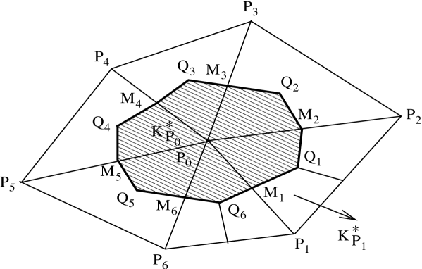
Figure 1.

We consider a finite volume element discretization of (1) in the standard $C^{0}$-conforming piecewise linear finite element space $U_{h}$ on the primary mesh $\mathcal{T}_{h}$, which is defined by

$$U_{h}=\{v_{h}\in C^{0}(\overline{\Omega})\;:\;v_{h}|_{K}\;\mbox{is linear for all}~{}K\in\mathcal{T}_{h}\;\mbox{and}\;v_{h}|_{\partial\Omega}=0\},$$

and the dual volume element space $U_{h}^{*}$ on the dual mesh $\mathcal{T}^{*}_{h}$ given by

$$U_{h}^{*}=\{v_{h}\in L^{2}(\Omega)\;:\;v_{h}|_{K_{P_{0}}^{*}}\;\mbox{is constant for all}\;K_{P_{0}}^{*}\in\mathcal{T}_{h}^{*}\;\mbox{and}\;v_{h}|_{\partial\Omega}=0\}.$$

Now, $U_{h}=\mbox{span}\{\phi_{i}\;:\;P_{i}\in N_{h}^{0}\}$ and $U_{h}^{*}=\mbox{span}\{\chi_{i}\;:\;P_{i}\in N_{h}^{0}\}$, where $\phi_{i}$’s are the standard nodal basis functions associated with nodes $P_{i}$ and $\chi_{i}$’s are the characteristic basis functions corresponding to the control volume $K_{P_{i}}^{*}$ given by

$$\chi_{i}(x)=\left\{\begin{array}[]{cc}1,&\mbox{if}~{}x\in K_{P_{i}}^{*}\\ 0,&\mbox{elsewhere}.\\ \end{array}\right.$$

The semidiscrete finite volume element formulation for (1) is to seek $u_{h}:(0,T]\longrightarrow U_{h}$ such that

$$(u_{h,tt},v_{h})+A_{h}(u_{h},v_{h})+\int_{0}^{t}B_{h}(t,s;u_{h}(s),v_{h})\,ds=(f,v_{h})\;\;\forall v_{h}\in U_{h}^{*},~{}~{}~{}~{}~{}~{}~{}~{}~{}~{}~{}~{}~{}~{}~{}~{}~{}~{}~{}~{}~{}$$ (3.3)

with given initial data $u_{h}(0)$ and $u_{h,t}(0)$ in $U_{h}$ to be defined later. Here, the bilinear forms $A_{h}(\cdot,\cdot)$ and $B_{h}(t,s;\cdot,\cdot)$ are defined, respectively, by

$$A_{h}(u_{h},v_{h})=-\sum_{P_{i}\in N_{h}^{0}}v_{h}(P_{i})\int_{\partial K_{P_{i}}^{*}}\mathcal{A}(x)\nabla u_{h}\cdot{\bf n}\,ds,~{}~{}~{}~{}$$

and

$$B_{h}(t,s;u_{h},v_{h})=-\sum_{P_{i}\in N_{h}^{0}}v_{h}(P_{i})\int_{\partial K_{P_{i}}^{*}}\mathcal{B}(x,t,s)\nabla u_{h}\cdot{\bf n}\,ds$$

for all $(u_{h},v_{h})\in U_{h}\times U_{h}^{*}$, with ${\bf n}$ denoting the outward unit normal to the boundary of the control volume $K_{P_{i}}^{*}$. Notice that by taking the $L^{2}$ inner product of (1) with $v_{h}\in U_{h}^{*}$ and then integrating, we obtain a similar equation for $u$ as

$$(u_{tt},v_{h})+A_{h}(u,v_{h})+\int_{0}^{t}B_{h}(t,s;u(s),v_{h})\,ds=(f,v_{h})\;\;\;\forall v_{h}\in U_{h}^{*}.$$ (3.4)

For the error analysis, we first introduce two interpolation operators. Let $\Pi_{h}:C(\Omega)\longrightarrow U_{h}$ be the piecewise linear interpolation operator and $\Pi_{h}^{*}:C(\Omega)\longrightarrow U_{h}^{*}$ be the piecewise constant interpolation operator. These interpolation operators are defined, respectively, by

$$\Pi_{h}u=\sum_{P_{i}\in N_{h}^{0}}u(P_{i})\phi_{i}(x)\;~{}\mbox{and}~{}\;\Pi_{h}^{*}u=\sum_{P_{i}\in N_{h}^{0}}u(P_{i})\chi_{i}(x).$$ (3.5)

Now for $\psi\in H^{2}$, $\Pi_{h}$ has the following approximation property, (see, Ciarlet [10]):

$$\|\psi-\Pi_{h}\psi\|_{0}\leq Ch^{2}\|\psi\|_{2}.$$ (3.6)

Further, we introduce the following discrete norms

$$\|v_{h}\|_{0,h}=\left(\sum_{K\in T_{h}}|v_{h}|_{0,h,K}^{2}\right)^{1/2}\;\;\mbox{and}\;\;\|v_{h}\|_{1,h}=\left(\|v_{h}\|_{0,h}^{2}+|v_{h}|_{1,h}^{2}\right)^{1/2},$$

where the seminorm $|v_{h}|_{1,h}=\left(\sum_{K\in T_{h}}|v_{h}|_{1,h,K}^{2}\right)^{1/2}$, and for $K=K_{Q}=\triangle P_{1}P_{2}P_{3}$,

$$|v_{h}|_{0,h,K}=\left\{\frac{1}{3}\left(v_{h}(P_{1})^{2}+v_{h}(P_{2})^{2}+v_{h}(P_{3})^{2}\right)\;|K|\;\right\}^{1/2}$$

$$|v_{h}|_{1,h,K}=\left\{(|\frac{\partial v_{h}}{\partial x}|^{2}+|\frac{\partial v_{h}}{\partial y}|^{2})\;|K|\;\right\}^{1/2}.$$

In the following Lemma, a relation between discrete norms and standard Sobolev norms is stated without proof. For a proof, see, [17, pp. 124] and [4].

Lemma 3.1

For $v_{h}\in U_{h},~{}|\cdot|_{1,h}$ and $|\cdot|_{1}$ are identical; $\|\cdot\|_{0,h}$ and $\|\cdot\|_{1,h}$ are equivalent to $\|\cdot\|_{0}$ and $\|\cdot\|_{1}$, respectively, that is, there exist positive constants $C_{3}$ and $C_{4}>0$, independent of h, such that

$$C_{3}\|v_{h}\|_{0,h}\leq\|v_{h}\|_{0}\leq C_{4}\|v_{h}\|_{0,h}\;\;\;\forall v_{h}\in U_{h}$$ (3.7)

and

$$C_{3}||v_{h}||_{1,h}\leq||v_{h}||_{1}\leq C_{4}||v_{h}||_{1,h}\;\;\;\;\forall v_{h}\in U_{h}.$$ (3.8)

Note that $\|v_{h}\|_{0,h}=\|\Pi_{h}^{*}v_{h}\|_{0}.$ Below, we state without proof the properties of the interpolation operator $\Pi_{h}^{*}.$ For a proof, we refer to [17, pp. 192].

Lemma 3.2

The following statements hold true.
$(i)\;\mbox{For}\;\;\Pi_{h}^{*}:U_{h}\longrightarrow U_{h}^{*}\mbox{ defined in (\ref{naa}),}\qquad\qquad\qquad\qquad\qquad$

$$(\phi_{h},\Pi_{h}^{*}v_{h})=(v_{h},\Pi_{h}^{*}\phi_{h})\;\;\;\;\;\forall\phi_{h},~{}v_{h}\in U_{h}.$$ (3.9)

(ii)  With $\||\phi_{h}\||:=(\phi_{h},\Pi_{h}^{*}\phi_{h})^{1/2}$, the norms $\||\cdot\||$ and $\|\cdot\|_{0}$ are equivalent on $U_{h}$, that is, there exist positive constants $c_{eq}$ and $C_{eq}$, independent of $h$, such that

$$c_{eq}||\phi_{h}||_{0}\leq\||\phi_{h}\||\leq C_{eq}||\phi_{h}||_{0}\;\;\;\;\;\;\;\forall\phi_{h}\in U_{h}.$$ (3.10)

4. A Priori Error Estimates

This section is devoted to a priori error estimates of the approximation $u_{h}$ to the spatial semidiscrete scheme (3.3).

For the derivation of optimal error estimates, we split $e=u-u_{h}$ as

$$e:=(u-V_{h}u)+(V_{h}u-u_{h})=:\rho+\theta,$$

where $V_{h}:L^{\infty}(H_{0}^{1}\cap H^{2})\rightarrow L^{\infty}(U_{h})$ is the Ritz-Volterra projection defined by

$$A(u-V_{h}u,\chi_{h})+\int_{0}^{t}B(t,s;u-V_{h}u,\chi_{h})\,ds=0\;\;\;\;\forall\chi_{h}\in U_{h}.$$ (4.1)

With some abuse of notations, we will denote by $V_{h}u_{0}$ the Ritz projection of $u_{0}$ onto $U_{h}$ defined by

$$A(u_{0}-V_{h}u_{0},\chi_{h})=0\;\;\;\;\forall\chi_{h}\in U_{h}.$$

For our subsequent analysis, we state without proof following error estimates for the Ritz-Volterra projection. For a proof, see, [26], [5], [18], [20] and [21].

Lemma 4.1

There exist positive constants $C$, independent of $h$, such that for $j=0,1,2$, and $r=1,2$ the following estimates hold:

$$\|D_{t}^{j}\rho(t)\|_{0}+h\|D_{t}^{j}\rho(t)\|_{1}\leq Ch^{r}\left[\sum_{l=0}^{j}\|D_{t}^{l}u(t)\|_{r}+\int_{0}^{t}\|u(s)\|_{r}\;ds\right],$$ (4.2)

and

$$\|\rho(t)\|_{0,\infty}\leq Ch^{2}\left(\log\frac{1}{h}\right)\left(\|u(t)\|_{2,\infty}+\int_{0}^{t}||u(s)||_{2,\infty}ds\right).$$ (4.3)

Now, define

$$\epsilon_{h}(f,\chi)=(f,\chi)-(f,\Pi_{h}^{*}\chi)\;\;\;\;\forall\chi\in U_{h},~{}~{}~{}~{}~{}~{}~{}~{}~{}~{}~{}~{}~{}~{}~{}$$

$$\;\;\;\;\;\;\;\;\;\;\;\;\;\epsilon_{A}(\psi,\chi)=A(\psi,\chi)-A_{h}(\psi,\Pi_{h}^{*}\chi)\;\;\;\;\forall\psi,~{}\chi\in U_{h},$$

and

$$\;\;\;\;\;\;\;\;\;\;\;\;\;\epsilon_{B}(t,s;\psi,\chi)=B(t,s;\psi,\chi)-B_{h}(t,s;\psi,\Pi_{h}^{*}\chi)\;\;\;\;\forall\psi,~{}\chi\in U_{h}.$$

Then, the following lemma will be of frequent use in our analysis and the proof of which can be found in [8].

Lemma 4.2

Assume that the coefficient matrices $\mathcal{A},\mathcal{B}(t,s)\in W^{1+i,\infty}(\Omega;\mathbb{R}^{2\times 2})$ for $i=0,1.$ Then, there exist positive constant $C,$ independent of $h$, such that the following estimates hold for $\chi\in U_{h}$ and for $i,~{}j=0,~{}1$

$$|\epsilon_{h}(f,\chi)|\leq Ch^{i+j}\|f\|_{H^{i}}\;\|\chi\|_{H^{j}}\;\;\;\forall f\in H^{i},$$ (4.4)

and for $u\in H^{1+i}\cap H_{0}^{1}$

$$|\epsilon_{A}(V_{h}u,\chi)|\leq Ch^{i+j}\Big{(}\|u\|_{H^{1+i}}+\int_{0}^{t}\|u(s)\|_{H^{1+i}}\;ds\Big{)}\;\|\chi\|_{H^{j}}.$$ (4.5)

Moreover,

$$|\epsilon_{A}(w_{h},\chi)|\leq Ch\|w_{h}\|_{H^{1}}\;\|\chi\|_{H^{1}}\;\forall w_{h}\in U_{h}.$$ (4.6)

The estimates (4.5) and (4.6) are also valid if $\epsilon_{A}$ is replaced by $\epsilon_{B}.$

Now, for $\psi\in H^{1}_{0}$ and for each $t\in(0,T],$ introduce a linear functional $G(\psi)=G(t,\psi)$ defined on $U_{h}$ by

$$G(\psi)(\chi)=\epsilon_{A}(\psi,\chi)+\int_{0}^{t}\epsilon_{B}(t,s;\psi(s),\chi)\,ds,\,\,\,\chi\in U_{h}.$$

Notice that, by using the definition of $G$, (2.1) and (3.4), there follows that

$$G(\rho)(\chi) = A(u,\chi)+\int_{0}^{t}B(t,s;u(s),\chi)\,ds$$ (4.7)

$$-A_{h}(u,\Pi_{h}^{*}\chi)-\int_{0}^{t}B_{h}(t,s;u(s),\Pi_{h}^{*}\chi)\,ds-G(V_{h}u)(\chi)$$

$$= (f-u_{tt},\chi)-(f-u_{tt},\Pi_{h}^{*}\chi)-G(V_{h}u)(\chi)$$

$$= \epsilon_{h}(f-u_{tt},\chi)-G(V_{h}u)(\chi).$$

From (3.3) and (3.4), we obtain the equation in $\theta$ for $v_{h}\in U_{h}^{*}$ as

$$(\theta_{tt},v_{h})+A_{h}(\theta,v_{h})+\int_{0}^{t}B_{h}(t,s;\theta(s),v_{h})\,ds=-A_{h}(\rho,v_{h})-\int_{0}^{t}B_{h}(t,s;\rho,\chi)\,ds-(\rho_{tt},v_{h}).$$

Choosing $v_{h}=\Pi_{h}^{*}\chi$ and using the definition of $G$ and (4.1), we find that

$$(\theta_{tt},\Pi_{h}^{*}\chi)+A(\theta,\chi)\;ds + \int_{0}^{t}B(t,s;\theta(s),\chi)\,ds=G(\rho)(\chi)$$ (4.8)

$$+ G(\theta)(\chi)-(\rho_{tt},\Pi_{h}^{*}\chi)\;\;\forall\chi\in U_{h}.$$

For any continuous function $\phi$ in $[0,t]$, define $\hat{\phi}$ by

$$\hat{\phi}(t)=\int_{0}^{t}\phi(s)\,ds.$$

Notice that $\hat{\phi}(0)=0$ and $(d\hat{\phi}/dt)(t)=\phi(t)$. Then, integrate (4.8) from $0$ to $t$ to obtain

$$(\theta_{t},\Pi_{h}^{*}\chi)+A(\hat{\theta},\chi) = \hat{G}(\rho)(\chi)+\hat{G}(\theta)(\chi)+(-\rho_{t},\Pi_{h}^{*}\chi)+(e_{t}(0),\Pi_{h}^{*}\chi)$$ (4.9)

$$-\int_{0}^{t}B(s,s;\hat{\theta}(s),\chi)ds+\int_{0}^{t}\int_{0}^{s}B_{\tau}(s,\tau;\hat{\theta}(\tau),\chi)d\tau ds,$$

where

$$\hat{G}(\phi)(\chi)=\epsilon_{A}(\hat{\phi},\chi)+\int_{0}^{t}\epsilon_{B}(s,s;\hat{\phi}(s),\chi)ds-\int_{0}^{t}\int_{0}^{s}\epsilon_{B_{\tau}}(s,\tau;\hat{\phi}(\tau),\chi)d\tau ds.$$

For a linear functional $F$ defined on $U_{h}$, set

$$\|F\|_{-1,h}=\sup_{0\neq\chi\in U_{h}}\frac{|F(\chi)|}{\|\chi\|_{1}}.$$

We shall need the following lemmas in our subsequent analysis.

Lemma 4.3

With $G$ and $\hat{G}$ as above, there exists a positive constant $C=C(T)$ such that the following estimates

$$\|D_{t}^{j}G(V_{h}u)\|_{-1,h}\leq Ch^{2}\left(\sum_{\ell=0}^{j}\|D^{\ell}_{t}u(t)\|_{2}+\int_{0}^{t}\|u(s)\|_{2}\,ds\right),$$ (4.10)

and

$$\|D_{t}^{j}\hat{G}(V_{h}u)\|_{-1,h}\leq Ch^{2}\left(\sum_{\ell=0}^{j}\|D^{j}_{t}\hat{u}(t)\|_{2}+\int_{0}^{t}\|\hat{u}(s)\|_{2}\;ds\right),$$ (4.11)

hold for $j=0,1$.

Proof. Using (4.5) and the estimates in Lemma 2.1, we obtain

$$|G(V_{h}u)(\chi)| \leq |\epsilon_{A}(V_{h}u,\chi)|+\int_{0}^{t}|\epsilon_{B}(t,s;V_{h}u(s),\chi)|\,ds$$

$$\leq Ch^{2}\left(\|u\|_{2}+\int_{0}^{t}\|u(s)\|_{2}\,ds\right)\|\chi\|_{1},$$

and

$$|G_{t}(V_{h}u)(\chi)| \leq Ch^{2}\left(\|u_{t}\|_{2}+\|u\|_{2}+\int_{0}^{t}\|u(s)\|_{2}\,ds\right)\|\chi\|_{1}$$

$$\leq Ch^{2}\left(\|u_{t}\|_{2}+\|u\|_{2}+\int_{0}^{t}\|u(s)\|_{2}\,ds\right)\|\chi\|_{1}$$

In a similar manner, we derive the second estimate (4.11) and this completes the rest of the proof.  

In the error analysis, we shall frequently use the following inverse assumption:

$$\|\chi\|_{1}\leq C_{inv}h^{-1}\|\chi\|_{0},\quad\chi\in U_{h}.$$ (4.12)

4.1. $H^{1}$- error estimate

Theorem 4.1

Let $u$ and $u_{h}$ be the solutions of $(\ref{a})$ and $(\ref{c}),$ respectively, and assume that $f\in L^{1}(H^{1}),\;f_{t},\;f_{tt}\in L^{1}(L^{2})$, $u_{0}\in H^{3}\cap H_{0}^{1}$ and $u_{1}\in H^{2}\cap H_{0}^{1}$. Further, assume that $u_{h}(0)=\Pi_{h}u_{0}$ and $u_{h,t}(0)=\Pi_{h}u_{1}$, where $\Pi_{h}$ is the interpolation operator defined in $(\ref{naa})$. Then, there exists a positive constant $C=C(T)$, independent of $h$, such that for $t\in(0,T]$ the following estimate

$$\|u(t)-u_{h}(t)\|_{1}\leq C\;h\left(\|u_{0}\|_{3}+\|u_{1}\|_{2}+\int_{0}^{t}\Big{(}\|f\|_{1}+\|f_{t}\|_{0}+\|f_{tt}\|_{0}\Big{)}\,ds\right)$$

holds.

Proof. Since $u-u_{h}=\rho+\theta$ and estimates of $\rho$ are known from the Lemma 4.1, it is sufficient to estimate $\theta.$ Choose $\chi=\theta_{t}$ in (4.8) and use (4.7) to obtain

$$(\theta_{tt},\Pi_{h}^{*}\theta_{t})+A(\theta,\theta_{t})+\int_{0}^{t}B(t,s;\theta(s),\theta_{t})\,ds = \epsilon_{h}(f-u_{tt},\theta_{t})-G(V_{h}u)(\theta_{t})$$

$$+G(\theta)(\theta_{t})-(\rho_{tt},\Pi_{h}^{*}\theta_{t}).$$

Now use (3.9) and symmetry of the bilinear form $A(\cdot,\cdot)$ to arrive at

$$\frac{1}{2}\frac{d}{dt}\Big{[}(\theta_{t},\Pi_{h}^{*}\theta_{t})+A(\theta,\theta)\Big{]} = \epsilon_{h}(f-u_{tt},\theta_{t})-G(V_{h}u)(\theta_{t})+G(\theta)(\theta_{t})-(\rho_{tt},\Pi_{h}^{*}\theta_{t})$$

$$-\int_{0}^{t}B(t,s;\theta(s),\theta_{t}(t))\,ds.$$

Integration from $0$ to $t$ yields

$$\frac{1}{2}\Big{(}\||\theta_{t}\||^{2}+A(\theta,\theta)\Big{)} = \frac{1}{2}\left(\||\theta_{t}(0)\||^{2}+A(\theta(0),\theta(0))\right)+\int_{0}^{t}\epsilon_{h}(f-u_{tt},\theta_{t})ds$$ (4.13)

$$-\int_{0}^{t}G(V_{h}u)(\theta_{t})ds+\int_{0}^{t}G(\theta)(\theta_{t})ds+\int_{0}^{t}(-\rho_{tt},\Pi_{h}^{*}\theta_{t})ds$$

$$-\int_{0}^{t}\int_{0}^{s}B(s,\tau;\theta(\tau),\theta_{t}(s))\,d\tau ds$$

$$= J_{1}+J_{2}+J_{3}+J_{4}+J_{5}+J_{6}.$$

For the first term on the right hand side of (4.13), a use of the boundedness of $A(\cdot,\cdot)$ with (3.6) and (3.10) shows

$$|J_{1}|\leq C\left(\|\theta_{t}(0)\|_{0}^{2}+\|\theta(0)\|_{1}^{2}\right)\leq Ch^{2}(\|u_{1}\|_{1}^{2}+\|u_{0}\|_{2}^{2}).$$ (4.14)

For estimating $J_{2},$ an application of (4.4) with $j=0$ implies

$$|J_{2}|\leq Ch\int_{0}^{t}\left(\|f\|_{1}+\|u_{tt}\|_{1}\right)\|\theta_{t}\|_{0}\;ds.$$ (4.15)

To estimate $J_{3}$, a use of the inverse inequality (4.12) shows that

$$|J_{3}|\leq C\int_{0}^{t}\|G(V_{h}u)\|_{-1,h}\|\theta_{t}\|_{1}\;ds\leq Ch^{-1}\int_{0}^{t}\|G(V_{h}u)\|_{-1,h}\|\theta_{t}\|_{0}\;ds.$$ (4.16)

Using the definition of $G$, (4.6) and the inverse inequality, it follows that

$$\;\;\;\;\;\;\;\;\;|J_{4}| \leq \int_{0}^{t}|G(\theta)(\theta_{t})|\;ds$$ (4.17)

$$\leq Ch\left[\int_{0}^{t}\|\theta\|_{1}\|\theta_{t}\|_{1}ds+\int_{0}^{t}\int_{0}^{s}\|\theta(\tau)\|_{1}\|\theta_{t}(s)\|_{1}d\tau ds\right]$$

$$\leq C\left[\int_{0}^{t}\|\theta\|_{1}\|\theta_{t}\|_{0}ds+\left(\int_{0}^{t}\|\theta\|_{1}ds\right)\left(\int_{0}^{t}\|\theta_{t}\|_{0}ds\right)\right].$$

For $J_{5}$, apply the Cauchy-Schwarz inequality, $L^{2}$ stability of $\Pi_{h}^{*}$ and (4.2) with $r=1$ to obtain

$$|J_{5}|\leq\int_{0}^{t}\|\rho_{tt}\|_{0}\;\|\theta_{t}\|_{0}\;ds\leq C(T)\;h\int_{0}^{t}\Big{(}\|u_{tt}\|_{1}+\|u_{t}\|_{1}+\|u\|_{1}\Big{)}\|\theta_{t}\|_{0}\;ds.$$ (4.18)

For the term $J_{6},$ we note that an integration by parts yields

$$\int_{0}^{t}\int_{0}^{s}B(s,\tau;\theta(\tau),\theta_{t}(s))\,d\tau\;ds = \int_{0}^{t}B(t,s;\theta(s),\theta(t))\,ds-\int_{0}^{t}B(s,s;\theta(s),\theta(s))$$

$$-\int_{0}^{t}\int_{0}^{s}B_{s}(s,\tau;\theta(\tau),\theta(s))\,d\tau\;ds,$$

and hence, deduce that

$$|J_{6}|\leq C\left(\|\theta(t))\|_{1}\;\int_{0}^{t}\|\theta(s)\|_{1}\,\;ds+\int_{0}^{t}\|\theta(s)\|^{2}_{1}\,ds\right).$$ (4.19)

Now, set $\mathcal{E}^{2}_{1}(t)=\|\theta_{t}\|^{2}_{0}+\|\theta\|^{2}_{1}$ and

$$\mathcal{E}_{1}(t^{\ast})=\max_{0\leq\tau\leq t}\mathcal{E}_{1}(t),$$

for some $t^{\ast}\in[0,t]$. Then, substituting the estimates (4.14)-(4.19) in (4.13), using coercivity of $A(\cdot,\cdot)$, equivalence of norms $\||\cdot\||$ and $\|\cdot\|_{0},$ apply standard kick back arguments to find that

$$\mathcal{E}_{1}(t^{\ast}) \leq Ch\;\Big{(}\|u_{0}\|_{2}+\|u_{1}\|_{1}+\int_{0}^{T}\left(\|u_{tt}(s)\|_{1}+\|u_{t}(s)\|_{1}+\|u(s)\|_{1}\right)\;ds\Big{)}$$

$$+ Ch\;\int_{0}^{T}\left(\|f(s)\|_{1}+h^{-2}\|G(V_{h}u)(s)\|_{-1,h}\right)\;ds+\int_{0}^{t^{\ast}}\mathcal{E}_{1}(s)\;ds.$$

Now replace $t^{\ast}$ by $t$ and apply Gronwall’s lemma with the estimate (4.10) to conclude that

$$\mathcal{E}_{1}(t)\leq~{}Ch\Big{(}\|u_{0}\|_{2}+\|u_{1}\|_{1}+\int_{0}^{T}\left(\|u\|_{2}+\|u_{t}\|_{1}+\|u_{tt}\|_{1}+\|f\|_{1}\right)\;ds\Big{)}.$$

A use of triangle inequality with (4.2) and the estimates from Lemma 2.1 completes the rest of the proof.  

4.2. Optimal $L^{2}$- error estimates

In this subsection, we shall discuss optimal $L^{\infty}(L^{2})$ estimates

Theorem 4.2

Under the assumptions of Theorem $\ref{H2},$ there exists a positive constant $C=C(T)$, independent of $h$, such that

$$\|u(t)-u_{h}(t)\|_{0}\leq Ch^{2}\left(\|u_{0}\|_{3}+\|u_{1}\|_{2}+\int_{0}^{t}\Big{(}\|f\|_{1}+\|f_{t}\|_{0}+\|f_{tt}\|_{0}\Big{)}\,ds\right).$$

Proof. By setting $\chi=\theta$ in (4.9), and using (3.9) with symmetry of the bilinear form $A(\cdot,\cdot)$, we find that

$$\frac{1}{2}\frac{d}{dt}\left[(\theta,\Pi_{h}^{*}\theta)+A(\hat{\theta},\hat{\theta})\right] = \hat{G}(\rho)(\theta)+\hat{G}(\theta)(\theta)+(-\rho_{t},\Pi_{h}^{*}\theta)+(u_{1}-\Pi_{h}u_{1},\Pi_{h}^{*}\theta)$$

$$-\int_{0}^{t}B(s,s;\hat{\theta}(s),\theta(t))\;ds+\int_{0}^{t}\int_{0}^{s}B_{\tau}(s,\tau;\hat{\theta}(\tau),\theta(t))\;d\tau\;ds.$$

Integrate from $0$ to $t$ to obtain

$$\frac{1}{2}\left[\||\theta\||^{2}+A(\hat{\theta},\hat{\theta})\right] = \frac{1}{2}\||\theta(0)\||^{2}+\int_{0}^{t}\hat{G}(\rho)(\theta)\;ds+\int_{0}^{t}\hat{G}(\theta)(\theta)\;ds+\int_{0}^{t}(-\rho_{t},\Pi_{h}^{*}\theta)\;ds$$ (4.20)

$$+(u_{1}-\Pi_{h}u_{1},\Pi_{h}^{*}\hat{\theta})-\int_{0}^{t}\int_{0}^{s}B(\tau,\tau;\hat{\theta}(\tau),\theta(s))\;d\tau\;ds$$

$$+\int_{0}^{t}\int_{0}^{s}\int_{0}^{\tau^{\prime}}B_{\tau^{\prime}}(\tau,\tau^{\prime};\hat{\theta}(\tau^{\prime}),\theta(s))\;d\tau^{\prime}\;d\tau\;ds$$

$$= \frac{1}{2}\||\theta(0)\||_{0}^{2}+I_{1}+I_{2}+I_{3}+I_{4}+I_{5}+I_{6}.$$

To estimate $I_{1}$, we note from (4.7) that

$$\hat{G}(\rho)(\theta) = \epsilon_{h}(\hat{f}-\hat{u}_{tt},\theta)-\hat{G}(V_{h}u)(\theta)$$ (4.21)

$$= \frac{d}{dt}\left(\epsilon_{h}(\hat{f}-\hat{u}_{tt},\hat{\theta})-\hat{G}(V_{h}u)(\hat{\theta})\right)-\Big{(}\epsilon_{h}({f}-{u}_{tt},\hat{\theta})-\hat{G}_{t}(V_{h}u)(\hat{\theta})\Big{)},$$

and hence,

$$I_{1}=\left(\epsilon_{h}(\hat{f}-\hat{u}_{tt},\hat{\theta})-\hat{G}(V_{h}u)(\hat{\theta})\right)-\int_{0}^{t}\left(\epsilon_{h}({f}-{u}_{tt},\hat{\theta})-\hat{G}_{s}(V_{h}u)(\hat{\theta})\right)ds.$$

A use of (4.4) for $j=1$ shows

$$|I_{1}| \leq |\epsilon_{h}(\hat{f}-({u}_{t}-u_{1}),\hat{\theta})|+|\hat{G}(V_{h}u)(\hat{\theta})|$$ (4.22)

$$+\int_{0}^{t}\left(|\epsilon_{h}({f}-{u}_{tt},\hat{\theta})|+|\hat{G}_{s}(V_{h}u)(\hat{\theta})|\right)\;ds$$

$$\leq C\left[h^{2}\left(\|\hat{f}\|_{1}+\|u_{t}\|_{1}+\|u_{1}\|_{1}\right)+\|\hat{G}(V_{h}u)\|_{-1,h}\right]\|\hat{\theta}\|_{1}$$

$$+C\int_{0}^{t}\left(h^{2}(\|f\|_{1}+\|u_{tt}\|_{1})+\|\hat{G}_{s}(V_{h}u)\|_{-1,h}\right)\|\hat{\theta}\|_{1}\;ds.$$

Notice that $I_{2}$ can be written as

$$I_{2} = \int_{0}^{t}\epsilon_{A}(\hat{\theta},\theta)ds+\int_{0}^{t}\int_{0}^{s}\epsilon_{B}(\tau,\tau;\hat{\theta}(\tau),\theta(s))\;d\tau\;ds$$ (4.24)

$$-\int_{0}^{t}\int_{0}^{s}\int_{0}^{\tau}\epsilon_{B_{\tau^{\prime}}}(\tau,\tau^{\prime};\hat{\theta}(\tau^{\prime}),\theta(s))\;d\tau^{\prime}\;d\tau\;ds$$

$$= I_{21}+I_{22}+I_{23}.$$ (4.25)

For $I_{21}$, we apply (4.6) and the inverse inequality (4.12) to find that

$$|I_{21}|=\int_{0}^{t}|\epsilon_{A}(\hat{\theta},\theta)|ds\leq Ch\int_{0}^{t}\|\theta\|_{1}\|\hat{\theta}\|_{1}\leq CC_{inv}\int_{0}^{t}\|\theta\|_{0}\;\|\hat{\theta}\|_{1}.$$ (4.26)

In order to estimate $I_{22}$, we integrate by parts in time so that

$$|I_{22}| = \left|\int_{0}^{t}\epsilon_{B}(s,s;\hat{\theta}(s),\hat{\theta}(t))\;ds-\int_{0}^{t}\epsilon_{B}(s,s;\hat{\theta}(s),\hat{\theta}(s))\;ds\right|$$

$$\leq Ch\left\{\|\hat{\theta}(t)\|_{1}\int_{0}^{t}\|\hat{\theta}(s)\|_{1}\;ds+\int_{0}^{t}\|\hat{\theta}(s)\|_{1}^{2}\;ds\right\}.$$

Similarly for $I_{23}$, we note that

$$|I_{23}| = \left|\int_{0}^{t}\int_{0}^{s}\epsilon_{B_{\tau}}(s,\tau;\hat{\theta}(\tau),\hat{\theta}(t))\;d\tau\;ds-\int_{0}^{t}\int_{0}^{s}\epsilon_{B_{\tau}}(s,\tau;\hat{\theta}(\tau),\hat{\theta}(s))\;d\tau\;ds\right|$$

$$\leq C(T)h\left\{\|\hat{\theta}(t)\|_{1}\int_{0}^{t}\|\hat{\theta}(s)\|_{1}\;ds+\int_{0}^{t}\|\hat{\theta}(s)\|_{1}^{2}\;ds\right\}.$$

Using stability of $\Pi_{h}^{*}$ (i.e., $\|\Pi_{h}^{*}\theta\|_{0}\leq C\|\theta\|_{0}$) and the Cauchy-Schwarz inequality, it follows that

$$|I_{3}|\leq\int_{0}^{t}|(\rho_{t},\Pi_{h}^{*}\theta)|ds\leq C\int_{0}^{t}\|\rho_{t}(s)\|_{0}\|\theta(s)\|_{0}ds.$$ (4.27)

For $I_{4}$, we apply (3.6) and $\|\Pi_{h}^{*}\hat{\theta}\|_{0}\leq C\|\hat{\theta}\|_{1}$ to obtain

$$|I_{4}|\leq\|u_{1}-\Pi_{h}u_{1}\|_{0}\;\|\Pi_{h}^{*}\hat{\theta}\|_{0}\leq Ch^{2}\|u_{1}\|_{2}\;\|\hat{\theta}\|_{1}.$$ (4.28)

Finally, similarly for $I_{22}$ and $I_{23}$, an integration by parts leads to

$$|I_{5}|+|I_{6}|\leq C(T)\left\{\|\hat{\theta}(t)\|_{1}\int_{0}^{t}\|\hat{\theta}(s)\|_{1}\;ds+\int_{0}^{t}\|\hat{\theta}(s)\|_{1}^{2}\;ds\right\}.$$ (4.29)

Now, define $\mathcal{E}_{0}^{2}(t)=\|\theta(t)\|^{2}_{0}+\|\hat{\theta}(t)\|^{2}_{1}$ and let $t^{\ast}\in[0,t]$ be such that

$$\mathcal{E}_{0}(t^{\ast})=\max_{0\leq s\leq t}\mathcal{E}_{0}(t).$$

At $t=t^{\ast}$, substitute the estimates (4.21)-(4.29) in (4.20) and use the equivalence of the norms $\||\cdot\||$ and $\|\cdot\|_{0}$ from (3.10) along with the coercivity property (2.2) of $A(\cdot,\cdot)$. Then a standard use of kick back arguments yields

$$\mathcal{E}_{0}(t^{\ast}) \leq C\|\theta(0)\|+Ch^{2}\left[\|u_{0}\|_{2}+\|u_{1}\|_{2}+\int_{0}^{t^{\ast}}\left(\|f\|_{1}+\|u_{tt}\|_{1}\right)\;ds\right]$$

$$+C\left[\|\hat{G}(V_{h}u)\|_{-1,h}+\int_{0}^{t^{\ast}}(\|\rho_{t}\|_{0}+\|\hat{G}_{s}(V_{h}u)\|_{-1,h})\;ds\right]+C\int_{0}^{t^{\ast}}\mathcal{E}_{0}(s)\;ds.$$

Note that $\|\theta(0)\|_{0}\leq Ch^{2}\|u_{0}\|_{2}$. Now apply Lemmas 4.3, 4.1 along with the estimates in Lemma 2.1 to obtain

$$\mathcal{E}_{0}(t^{\ast}) \leq Ch^{2}\left(\|u_{0}\|_{3}+\|u_{1}\|_{2}+\int_{0}^{t^{\ast}}\left(\|f\|_{1}+\|f_{t}\|_{0}+\|f_{tt}\|_{0}\right)\;ds\right)$$

$$+C\int_{0}^{t^{\ast}}\mathcal{E}_{0}(s)\;ds.$$

Then replace $t^{\ast}$ by $t$ and use Gronwall’s lemma for $t\leq T$ to conclude that

$$\|\theta(t)\|_{0}\leq C(T)h^{2}\left(\|u_{0}\|_{3}+\|u_{1}\|_{2}++\int_{0}^{T}\left(\|f\|_{1}+\|f_{t}\|_{0}+\|f_{tt}\|_{0}\right)ds\right).$$

Finally, a use of the triangle inequality completes the proof.  

Remark 4.1.

Note that it is possible to choose $u_{h,t}(0)$ as the $L^{2}$- projection of $u_{1}$ onto $U_{h}^{*}$ and in that case, the term $(u_{t}(0)-u_{h,t}(0),\Pi_{h}^{*}\theta_{t})$ becomes zero.

4.3. Maximum norm estimates

In this subsection, a superconvergent result for $\|\theta\|_{1}$ is first derived and it is then used to analyze quasi-optimal maximum error estimates.

Lemma 4.4

Assume that $f\in L^{1}(H^{2}),\;f_{t}\in L^{1}(H^{1}),\;f_{tt},\;f_{ttt}\in L^{1}(L^{2}),\;u_{0}\in H^{4}\cap H_{0}^{1}$ and $u_{1}\in H^{3}\cap H_{0}^{1}$. With $u_{h}(0)=V_{h}u_{0}$ and $u_{h,t}(0)=\Pi_{h}u_{1}$, there exists a positive constant $C=C(T),$ independent of $h,$ such that the following holds for $t\in(0,T]$

$$\|\theta_{t}(t)\|_{0}+\|{\theta}(t)\|_{1}\leq C\;h^{2}\Big{(}\|u_{0}\|_{4}+\|u_{1}\|_{3}+\|D_{t}^{3}f\|_{L^{1}(L^{2})}+\sum_{j=0}^{2}\|D_{t}^{j}f\|_{L^{1}(H^{2-j})}\Big{)}.$$

Proof. We now modify the estimates of $J_{1}$, $J_{2}$, $J_{3}$ and $J_{5}$ in (4.13) of Theorem  4.1 to obtain a superconvergence result for $\|\theta(t)\|_{1}$ norm. As $u_{h}(0)=V_{h}u_{0},$ it follows that $A(\theta(0),\theta(0))=0.$ Now with $u_{h,t}(0)=\Pi_{h}u_{1}$, we obtain

$$|J_{1}|\leq Ch^{4}\|u_{1}\|_{2}^{2}.$$ (4.30)

To estimate $J_{2}$, observe that

$$\epsilon_{h}(f-u_{tt},\theta_{t})=\frac{d}{dt}\epsilon_{h}(f-u_{tt},\theta)-\epsilon_{h}(f_{t}-u_{ttt},\theta),$$

and thus, rewrite $J_{2}$ as

$$J_{2}=\epsilon_{h}(f-u_{tt},\theta)-\int_{0}^{t}\epsilon_{h}(f_{t}-u_{ttt},\theta)ds.$$

Then, a use of (4.4) yields

$$|J_{2}|\leq Ch^{2}\Big{[}\left(\|f\|_{1}+\|u_{tt}\|_{1}\right)\|\theta\|_{1}+\int_{0}^{t}\left(\|f_{t}\|_{1}+\|u_{ttt}\|_{1}\right)\|\theta\|_{1}ds\Big{]}.$$ (4.31)

For $J_{3}$, rewrite $G$ term as

$$G(V_{h}u)(\theta_{t})=\frac{d}{dt}\left\{G(V_{h}u)(\theta)\right\}-G_{t}(V_{h}u)(\theta),$$

and hence, a use of (4.5) shows that

$$|J_{3}| \leq |G(V_{h}u)(\theta)|+\int_{0}^{t}|G_{s}(V_{h}u)(\theta)|\;ds$$ (4.32)

$$\leq 2\left[\|G(V_{h}u)\|_{-1,h}+\int_{0}^{t}\|G_{s}(V_{h}u)\|_{-1,h}\;ds\right]\|\theta\|_{1}.$$

For $J_{5}$, apply (4.2) to obtain

$$|J_{5}|\leq 2\int_{0}^{t}\|\rho_{tt}\|_{0}\|\theta_{t}\|_{0}ds\leq C(T)h^{2}\int_{0}^{t}\left(\|u_{tt}\|_{2}+|u_{t}\|_{2}+\|u\|_{2}\right)\,\|\theta_{t}\|_{0}\,ds.$$ (4.33)

Substituting the estimates (4.30)-(4.33) in (4.13), and apply standard kick back arguments to arrive at

$$\mathcal{E}_{1}(t) \leq Ch^{2}\Big{[}\|u_{1}\|_{2}+\|f\|_{1}+\|u_{tt}\|_{1}+|u_{t}\|_{2}+\|u\|_{2}$$

$$+\int_{0}^{t}\left(\|f_{t}\|_{1}+\|u\|_{2}+\|u_{t}\|_{2}+\|u_{tt}\|_{2}+\|u_{ttt}\|_{1}\right)ds\Big{]}$$

$$+C\int_{0}^{t}\mathcal{E}_{1}(s)\;ds.$$

An application of the integral identity (2.3) shows

$$\|f\|_{1}\leq\|f(0)\|_{1}+\int_{0}^{t}\|f_{t}\|_{1}ds.$$

Then using the estimates in Lemma 2.1 we arrive at

$$\mathcal{E}_{1}(t) \leq ~{}Ch^{2}\displaystyle\Big{(}\|u_{1}\|_{3}+\|u_{0}\|_{4}+\|f(0)\|_{1}$$

$$+\int_{0}^{T}\left(\|f\|_{2}+\|f_{t}\|_{1}+\|f_{tt}\|_{0}+\|f_{ttt}\|_{0}\right)ds\Big{)}$$

$$+C\int_{0}^{t}\mathcal{E}_{1}(s)\;ds.$$

Since $W^{1,1}([0,T];H^{1})$ is continuously imbedded in $C^{0}([0,T];H^{1})$, that is $\|f(0)\|_{1}\leq C\|f\|_{W^{1,1}(H^{1})}$, a use of Gronwall’s lemma completes the rest of the proof.  

Remark 4.2.

As a result of Lemma 4.4, we obtain a super-convergence estimate for $\theta$ in $H^{1}$-norm.

For $\|\theta\|_{\infty},$ a use of Sobolev inequality

$$\|\chi\|_{\infty}\leq C\left(\log\frac{1}{h}\right)^{1/2}\|\nabla\chi\|~{}~{}~{}~{}~{}~{}\forall\chi\in U_{h}$$ (4.34)

with Lemma 4.4 yields

$$\|{\theta}\|_{\infty} \leq C(T)h^{2}\left(\log\frac{1}{h}\right)^{1/2}\Big{[}\|u_{0}\|_{4}+\|u_{1}\|_{3}$$ (4.35)

$$+\int_{0}^{T}\left(\|f\|_{2}+\|f_{t}\|_{1}+\|f_{tt}\|_{0}+\|f_{ttt}\|_{0}\right)ds\Big{]}.$$

Below, we discuss the maximum norm estimate in form of a theorem.

Theorem 4.3

Let $u$ and $u_{h}$ be the solutions of $(\ref{a})$ and $(\ref{c})$ respectively. Further, let the assumptions of Lemma 4.4 hold. Then,

$$\|u(t)-u_{h}(t)\|_{\infty} \leq C\;h^{2}\left(\log\frac{1}{h}\right)\;\Big{(}\|u_{0}\|_{4}+\|u_{1}\|_{3}+\|D_{t}^{3}f\|_{L^{1}(L^{2})}$$

$$+\sum_{j=0}^{2}\|D_{t}^{j}f\|_{L^{1}(H^{2-j})}\Big{)},$$

where $C=C(T)$ is a positive constant independent of $h$.

Proof. By the triangle inequality

$$\|u(t)-u_{h}(t)\|_{\infty}\leq\|{\theta}\|_{\infty}+\|{\rho}\|_{\infty}.$$

Now, combine the estimates obtained in (4.35) and in (4.3) with Lemma 2.1 to obtain the required result.  

5. Error Estimates for a Completely Discrete Scheme

In this section, we introduce further notations and formulate a completely discrete scheme by applying an explicit finite difference method to discretize the time variable of the semidiscrete system (3.3). Then, we discuss optimal error estimates.

Let $k$ $(0<k<1)$ be the time step, $k=T/N$ for some positive integer $N$, and $t_{n}=nk$. For any function $\phi$ of time, let $\phi^{n}$ denote $\phi(t_{n})$. We shall use this notation for functions defined for continuous in time as well as those defined for discrete in time. Set $\phi^{n+1/2}=(\phi^{n+1}+\phi^{n})/2,$ and define the following notations for the difference quotients:

$${\delta}_{t}\phi^{n}=\frac{\phi^{n+1}-\phi^{n-1}}{2k},\quad{\partial}_{t}\phi^{n+1/2}=\frac{\phi^{n+1}-\phi^{n}}{k},\quad{\partial}_{t}^{2}\phi^{n}=\frac{\phi^{n+1}-2\phi^{n}+\phi^{n-1}}{k^{2}}.$$

Note that

$${\delta}_{t}\phi^{n}=\frac{{\partial}_{t}\phi^{n+1/2}+{\partial}_{t}\phi^{n-1/2}}{2},\qquad{\partial}_{t}^{2}\phi^{n}=\frac{{\partial}_{t}\phi^{n+1/2}-{\partial}_{t}\phi^{n-1/2}}{k}.$$

Then, the discrete-in-time scheme of (3.3) is to seek $U^{n}\in U_{h}$ such that for $\chi\in U_{h}$

$$\frac{2}{k}({\partial}_{t}U^{{1/2}},\Pi_{h}^{*}\chi)+A_{h}(U^{0},\Pi_{h}^{*}\chi)=(f^{0}+\frac{2}{k}u_{1},\Pi_{h}^{*}\chi),\quad\forall\chi\in U_{h},$$ (5.1)

$$({\partial}_{t}^{2}U^{n},\Pi_{h}^{*}\chi)+A_{h}(U^{n},\Pi_{h}^{*}\chi)+k\sum_{j=0}^{n-1}B_{h}(t_{n},t_{j+1/2};U^{j+1/2},\Pi_{h}^{*}\chi)=(f^{n},\Pi_{h}^{*}\chi),$$ (5.2)

$n\geq 1$, with a given initial data $U^{0}$ in $U_{h}$. This choice of time discretization leads to a second order accuracy in $k$. The integral term in (3.3) is computed by using the second order quadrature formula

$$\sigma^{n}(g)=k\sum_{j=0}^{n-1}g(t_{j+1/2})\approx\int_{0}^{t_{n}}g(s)\,ds,\quad\mbox{with}\quad t_{j+1/2}=(j+1/2)k.$$

We shall use a shorthand notation $\sigma^{n}(B_{h}^{n}(U,\Pi_{h}^{*}\chi))$ for $k\sum_{j=0}^{n-1}B_{h}(t_{n},t_{j+1/2};U^{j+1/2},\Pi_{h}^{*}\chi)$. The quadrature error $q^{n}(g)$ is defined by

$$q^{n}(g)=\sigma^{n}(g)-\int_{0}^{t_{n}}g(s)\,ds=\sum_{j=0}^{n-1}\left(kg^{j+{1/2}}-\int_{t_{j}}^{t_{j+1}}g(s)\,ds\right).$$

Similarly, for ${\phi}\in U_{h}$, we define a linear functional $q_{B}^{n}({\phi})$ representing the error in the quadrature formula by

$$q_{B}^{n}({\phi})({\chi})=\sigma^{n}\left(B^{n}({\phi},{\chi})\right)-\int_{0}^{t_{n}}B(t_{n},s;{\phi}(s),{\chi})\,ds.$$

Notice that $q_{B}^{0}({\phi})=0$.

For our future use, we state without proof the following lemma. For a proof, see, [21].

Lemma 5.1

There exists a positive constant $C,$ independent of $k$ and $h,$ such that the following estimate holds:

$$k\sum_{n=0}^{m}||{\partial}_{t}q_{B}^{n+1/2}({\phi})||_{-1,h}\leq Ck^{2}\int_{0}^{t_{m+1}}(||{\phi}||_{1}+||{\phi}_{t}||_{1}+||{\phi}_{tt}||_{1})\,ds.$$

Now, define $e^{n}:=u^{n}-U^{n}$. We split $e^{n}=\rho^{n}+\xi^{n}$ with $\rho^{n}=u^{n}-V_{h}u^{n}$ and $\xi^{n}=V_{h}u^{n}-U^{n}$. From (5.1)-(5.2) and (3.3), we derive equations in $e^{n}$ as follows

$$\frac{2}{k}({\partial}_{t}e^{{1/2}},\Pi_{h}^{*}\chi)+A_{h}(e^{0},\Pi_{h}^{*}\chi)=(2r^{0},\Pi_{h}^{*}\chi),$$ (5.3)

$$({\partial}_{t}^{2}e^{n},\Pi_{h}^{*}\chi)+A_{h}(e^{n},\Pi_{h}^{*}\chi)+\sigma^{n}\left(B_{h}^{n}(e,\Pi_{h}^{*}\chi\right)=(r^{n},\Pi_{h}^{*}\chi)+q_{B_{h}}^{n}(u)(\Pi_{h}^{*}\chi),$$ (5.4)

$n\geq 1$, for all $\chi\in U_{h}$, where $\displaystyle r^{0}=\frac{1}{k}\left({\partial}_{t}u^{1/2}-u_{1}\right)-\frac{1}{2}u_{tt}^{0}=\frac{1}{2k^{2}}\int_{0}^{k}(t-k)^{2}\frac{\partial^{3}u}{\partial t^{3}}(t)\,dt,$ and

$$r^{n}={\partial}_{t}^{2}u^{n}-u_{tt}^{0}=-\frac{1}{6k^{2}}\\ \int_{-k}^{k}(|t|-k)^{3}\frac{\partial^{4}u}{\partial t^{4}}(t^{n}+t)\,dt,\;\;n\geq 1.$$ (5.5)

Since estimates for $\rho$ are known from Lemma 4.1, it is sufficient to estimate $\xi$. From (5.3)-(5.4), we obtain the following equations in $\xi^{n}$:

$$\frac{2}{k}({\partial}_{t}\xi^{1/2},\Pi_{h}^{*}\chi) + A(\xi^{0},\chi)=-\frac{2}{k}({\partial}_{t}\rho^{{1/2}},\Pi_{h}^{*}\chi)+(2r^{0},\Pi_{h}^{*}\chi)$$ (5.6)

$$+ \epsilon_{h}(f^{0}-u_{tt}^{0},\chi)-\epsilon_{A}(V_{h}u(0),\chi),$$

$$({\partial}_{t}^{2}\xi^{n},\Pi_{h}^{*}\chi) + A(\xi^{n},\chi)=(r^{n},\Pi_{h}^{*}\chi)-({\partial}_{t}^{2}\rho^{n},\Pi_{h}^{*}\chi)+H^{n}(\xi)(\chi)$$ (5.7)

$$- \sigma^{n}\left(B^{n}(\xi,\chi)\right)-H^{n}(V_{h}u)(\chi)+\epsilon_{h}(f^{n}-u_{tt}^{n},\chi)+q^{n}_{B}(V_{h}u)(\chi),$$

where

$$H^{n}(\xi)(\chi)=\epsilon_{A}(\xi^{n},\chi)+k\sum_{j=0}^{n-1}\epsilon_{B}(t_{n},t_{j+1/2};\xi^{j+1/2},\chi).$$

Below, we shall obtain $l^{\infty}(H^{1})$-estimate for $\xi^{n+1/2}$.

Lemma 5.2

Assume that $f\in L^{1}(H^{2}),\;f_{t}\in L^{1}(H^{1}),\;f_{tt},\;f_{ttt}\in L^{1}(L^{2}),\;u_{0}\in H^{4}\cap H_{0}^{1}$ and $u_{1}\in H^{3}\cap H_{0}^{1}$. Further, assume that the CFL condition

$$\frac{k^{2}}{h^{2}}\leq\frac{4c_{eq}}{\Lambda C_{inv}}$$ (5.8)

is satisfied, where $\Lambda>0$ is the constant given in $(\ref{eqn2.3})$, $C_{inv}$ appears in the inverse inequality $(\ref{inv})$ and $c_{eq}$ is stated in the equivalence of norms as in $(\ref{nd})$. Then, with $u_{h}(0)=V_{h}u_{0}$ and $u_{h,t}(0)=\Pi_{h}u_{1},$ there exists a positive constant $C=C(T),$ independent of $h$ and $k$, such that the following estimate

$$\|{\partial}_{t}\xi^{m+1/2}\|_{0}+\|\xi^{m+1/2}\|_{1} \leq C(T)(k^{2}+h^{2})\Big{(}\|u_{0}\|_{4}+\|u_{1}\|_{3}$$ (5.9)

$$+\|D_{t}^{3}f\|_{L^{1}(L^{2})}+\sum_{j=0}^{2}\|D_{t}^{j}f\|_{L^{1}(H^{2-j})}\Big{)},$$

holds for $m=0,1,\cdots,N-1$.

Proof. Choose $\chi={\delta}_{t}\xi^{n}$ in (5.7) and obtain

$$\frac{1}{2}\bar{\partial}_{t}\Big{(}|||{\partial}_{t}\xi^{n+{1/2}}|||_{0}^{2} + A(\xi^{n+1},\xi^{n})\Big{)}=(r^{n}-{\partial}_{t}^{2}\rho^{n},\delta_{t}\xi^{n})+H^{n}(\xi)(\delta_{t}\xi^{n})$$

$$-\sigma^{n}\left(B^{n}(\xi,\delta_{t}\xi^{n})\right)-H^{n}(V_{h}u)(\delta_{t}\xi^{n})$$

$$+\epsilon_{h}(f^{n}-u_{tt}^{n},\delta_{t}\xi^{n})+q^{n}_{B}(V_{h}u)(\delta_{t}\xi^{n})$$

$$= I_{1}^{n}+I_{2}^{n}+I_{3}^{n}+I_{4}^{n}+I_{5}^{n}+I_{6}^{n},$$

where $\bar{\partial}_{t}$ denotes backward differencing. Next multiply (5) by $2k$ and sum the resulting one from $n=2$ to $m$ to arrive at

$$\frac{1}{2}\Big{(}|||{\partial}_{t}\xi^{m+1/2}|||_{0}^{2}+A(\xi^{m+1},\xi^{m})\Big{)} \leq \frac{1}{2}\Big{(}|||{\partial}_{t}\xi^{3/2}|||_{0}^{2}+A(\xi^{2},\xi^{1})\Big{)}$$ (5.11)

$$+k\left|\sum_{n=2}^{m}(I_{1}^{n}+I_{2}^{n}+I_{3}^{n}+I_{4}^{n}+I_{5}^{n}+I_{6}^{n})\right|.$$

Now define

$$|||\xi^{n+1/2}|||_{1}^{2}=||{\partial}_{t}\xi^{n+1/2}||_{0}^{2}+||\xi^{n+1/2}||_{1}^{2},$$

and let for some $m^{\star}$ with $0\leq m^{\star}\leq m,$

$$|||\xi^{m^{\star}+1/2}|||_{1}=\max_{0\leq n\leq m}|||\xi^{n+1/2}|||_{1}.$$

To estimate the sum in $I_{1}^{n}$, an application of the Cauchy-Schwarz inequality yields

$$k\left|\sum_{n=2}^{m}I_{1}^{n}\right| \leq Ck\sum_{n=2}^{m}\left(\|\partial^{2}_{t}\rho^{n}\|_{0}+\|r^{n}\|_{0}\right)\,\left(\|{\partial}_{t}\xi^{n+1/2}\|_{0}+\|{\partial}_{t}\xi^{n-1/2}\|_{0}\right)$$

$$\leq 2Ck\sum_{n=2}^{m}\left(\|\partial^{2}_{t}\rho^{n}\|_{0}+\|r^{n}\|_{0}\right)|||\xi^{m^{\star}+1/2}|||_{1}.$$

For the second sum on the right hand side of (5.11), we use the fact that

$$\psi^{n}{\delta}_{t}\xi^{n} = \bar{\partial}_{t}(\psi^{n}\xi^{n+1/2})-{\partial}_{t}\psi^{n+1/2}\xi^{n-1/2}$$ (5.12)

and conclude

$$k\sum_{n=2}^{m}\epsilon_{A}(\xi^{n},{\delta}_{t}\xi^{n})=\epsilon_{A}(\xi^{m},\xi^{m+1/2})-\epsilon_{A}(\xi^{1},\xi^{1+1/2})-k\sum_{n=2}^{m}\epsilon_{A}({\partial}_{t}\xi^{n+1/2},\xi^{n-1/2}).$$

Using (4.6) and the inverse inequality (4.12), we obtain

$$\left|k\sum_{n=2}^{m}\epsilon_{A}(\xi^{n},{\delta}_{t}\xi^{n})\right| \leq Ch\left\{\|\xi^{m}\|_{1}\|\xi^{m+1/2}\|_{1}+\|\xi^{1}\|_{1}\|\xi^{1+1/2}\|_{1}\right\}$$

$$+Chk\sum_{n=2}^{m}\|{\partial}_{t}\xi^{n+1/2}\|_{1}\|\xi^{n-1/2}\|_{1}$$

$$\leq C\left\{\|\xi^{m}\|_{0}+\|\xi^{1}\|_{0}+k\sum_{n=2}^{m}\|{\partial}_{t}\xi^{n+1/2}\|_{0}\right\}|||\xi^{m^{\star}+1/2}|||_{1}.$$

Since $\xi^{0}=0$, $\xi^{m}=k\sum_{n=0}^{m-1}{\partial}_{t}\xi^{n+1/2}$, and it follows that

$$\left|k\sum_{n=2}^{m}\epsilon_{A}(\xi^{n},{\delta}_{t}\xi^{n})\right|\leq Ck\left(\sum_{n=0}^{m-1}\|{\partial}_{t}\xi^{n+1/2}\|_{0}\right)|||\xi^{m^{\star}+1/2}|||_{1}.$$

Similarly, we obtain

$$\left|k^{2}\sum_{n=2}^{m}\sum_{j-0}^{n-1}\epsilon_{B}(t_{n},t_{j+1/2};\xi^{j+1/2},{\delta}_{t}\xi^{n})\right| \leq k^{2}\sum_{n=2}^{m}\left(C\sum_{j=0}^{n-1}\|\xi^{j+1/2}\|_{1}\right)|||\xi^{m^{\star}+1/2}|||_{1}$$

$$\leq CTk\left(\sum_{j=0}^{m-1}\|\xi^{j+1/2}\|_{1}\right)|||\xi^{m^{\star}+1/2}|||_{1},$$

and hence,

$$k\left|\sum_{n=2}^{m}I_{2}^{n}\right|\leq C(T)k\left(\sum_{n=0}^{m-1}|||\xi^{n+1/2}|||_{1}\right)|||\xi^{m^{\star}+1/2}|||_{1}.$$

To estimate the sum in $I_{3}^{n}$, we again use (5.12) and rewrite the sum as:

$$k\sum_{n=2}^{m}I_{3}^{n} = \sigma^{m}\left(B^{m}(\xi,\xi^{m+1/2})\right)-\sigma^{1}\left(B^{1}(\xi,\xi^{1+1/2})\right)$$

$$-k^{2}\sum_{n=2}^{m}\sum_{j=0}^{n-1}(\bar{\partial}_{t,1}B)(t_{n},t_{j+1/2};\xi^{j+1/2},\xi^{n-1/2})$$

$$+k\sum_{n=2}^{m}B(t_{n-1},t_{n-1/2};\xi^{n-1/2},\xi^{n-1/2}),$$

where $\bar{\partial}_{t,1}B$ denotes the difference quotient of $B$ with respect to its first argument. Since, $|\bar{\partial}_{t,1}B|\leq C||B_{t}||_{\infty}<\infty$, it follows that

$$\left|k\sum_{n=2}^{m}I_{3}^{n}\right|\leq C(T)k\left(\sum_{j=0}^{m-1}||\xi^{j+1/2}||_{1}\right)|||\xi^{m^{\star}+1/2}|||_{1}.$$

For the sum involving $I_{4}^{n}$, we note that

$$\left|k\sum_{n=2}^{m}\epsilon_{A}(V_{h}u^{n},{\delta}_{t}\xi^{n})\right| = \left|\epsilon_{A}(V_{h}u^{m},\xi^{m+1/2})-\epsilon_{A}(V_{h}u^{1},\xi^{1+1/2})-k\sum_{n=2}^{m}\epsilon_{A}({\partial}_{t}V_{h}u^{n+1/2},\xi^{n-1/2})\right|$$

$$\leq Ch^{2}\left\{||u^{m}||_{2}+||u^{1}||_{2}+k\sum_{n=0}^{m}||{\partial}_{t}V_{h}u^{n+1/2}||_{2}\right\}|||\xi^{m^{\star}+1/2}|||_{1}$$

$$\leq Ch^{2}\left\{||u_{0}||_{2}+||u_{t}||_{L^{1}(H^{2})}\right\}|||\xi^{m^{\star}+1/2}|||_{1}.$$

Similarly, we have

$$\left|k^{2}\sum_{n=2}^{m}\sum_{j=0}^{n-1}\epsilon_{B}(t_{n},t_{j+1/2};V_{h}u^{j+1/2},{\delta}_{t}\xi^{n})\right|\leq CTh^{2}\left\{||u_{0}||_{2}+||u_{t}||_{L^{1}(H^{2})}\right\}|||\xi^{m^{\star}+1/2}|||_{1}.$$

In order to estimate the sum in $I_{5}^{n}$, we repeat the previous arguments and use (4.4) to arrive at

$$\left|k\sum_{n=2}^{m}\epsilon_{h}(f^{n}-u^{n}_{tt},{\delta}_{t}\xi^{n})\right| = \left|\epsilon_{h}(f^{m}-u^{m}_{tt},\xi^{m+1/2})-\epsilon_{h}(f^{1}-u^{1}_{tt},\xi^{1+1/2})\right.$$

$$\left.-k\sum_{n=2}^{m}\epsilon_{h}\left({\partial}_{t}(f^{n+1/2}-u^{n+1/2}_{tt}),\xi^{n-1/2}\right)\right|$$

$$\leq Ch^{2}\left\{\|f^{0}-u_{tt}^{0}\|_{1}+\|f_{t}-u_{ttt}\|_{L^{1}(H^{1})}\right\}|||\xi^{m^{\star}+1/2}|||_{1}.$$

For the last sum, we rewrite it as

$$k\sum_{n=2}^{m}I_{6}^{n}=q^{m}_{B}(V_{h}u)(\xi^{m+1/2})-q^{1}_{B}(V_{h}u)(\xi^{1+1/2})-k\sum_{n=2}^{m}({\partial}_{t}q^{n+1/2}_{B}(V_{h}u))(\xi^{n-1/2}).$$

Since $q^{0}_{B}(V_{h}u)=0$, $q^{m}_{B}(V_{h}u)=k\sum_{n=0}^{m}{\partial}_{t}q^{n+1/2}_{B}(V_{h}u)$, we obtain

$$k\left|\sum_{n=2}^{m}I_{6}^{n}\right|\leq Ck\left\{\sum_{n=0}^{m}||{\partial}_{t}q^{n+1/2}_{B}(V_{h}u)||_{-1,h}\right\}|||\xi^{m^{\star}+1/2}|||_{1}.$$

Combining all the previous estimates, we conclude that

$$|||{\partial}_{t}\xi^{m+1/2}|||_{0}^{2}+A(\xi^{m+1},\xi^{m}) \leq |||{\partial}_{t}\xi^{3/2}|||_{0}^{2}+A(\xi^{2},\xi^{1})+Ck\left\{\sum_{n=2}^{m}(\|\partial^{2}_{t}\rho^{n}\|_{0}+\|r^{n}\|_{0})\right.$$ (5.13)

$$+ \left.\sum_{n=0}^{m}||{\partial}_{t}q^{n+1/2}_{B}(V_{h}u)||_{-1,h}+\sum_{j=0}^{m-1}|||\xi^{j+1/2}|||_{1}\right\}|||\xi^{m^{\star}+1/2}|||_{1}$$

$$+ h^{2}C(T,f,u)|||\xi^{m^{\star}+1/2}|||_{1},$$

where

$$C(T,f,u)=||u_{0}||_{2}+||u_{t}||_{L^{1}(H^{2})}+||u_{tt}(0)||_{1}+||u_{ttt}||_{L^{1}(H^{1})}+||f^{0}||_{1}+||f_{t}||_{L^{1}(H^{1})}.$$

In order to estimate the first two terms on the right hand side of (5.13), we choose $\chi={\partial}_{t}\xi^{3/2}$ in (5.7) for $n=1$ and obtain

$$|||{\partial}_{t}\xi^{3/2}|||_{0}^{2}+A(\xi^{2},\xi^{1}) \leq |||{\partial}_{t}\xi^{1/2}|||_{0}^{2}+h^{2}\Big{(}\|u^{1}\|_{2}+\|u_{0}\|_{2}+k\|{\partial}_{t}u^{1/2}\|_{2}\Big{)}$$

$$+ h^{2}\Big{(}\|f^{0}-u_{tt}^{0}\|_{2}+\|f_{t}-u_{ttt}\|_{L^{1}(0,k;H^{1})}\Big{)}+\|{\partial}_{t}q^{1/2}_{B}\|_{-1,h}.$$

Next, we choose $\chi={\partial}_{t}\xi^{1/2}$ in (5.6) to find that

$$|||{\partial}_{t}\xi^{1/2}|||_{0}\leq C\left\{\|{\partial}_{t}\rho^{1/2}\|_{0}+k\|r^{0}\|_{0}+h^{2}\|f^{0}-u_{tt}^{0}\|_{2}+h^{2}\|u_{0}\|_{2}\right\}.$$

A use of these estimates in (5.13) results in

$$|||{\partial}_{t}\xi^{m+1/2}|||_{0}^{2} + A(\xi^{m+1},\xi^{m})\leq C\left\{\|{\partial}_{t}\rho^{1/2}\|_{0}+k\sum_{n=1}^{m}\|\partial^{2}_{t}\rho^{n}\|_{0}+k\sum_{n=0}^{m}\|r^{n}\|_{0}\right.$$ (5.14)

$$\left.+k\sum_{n=0}^{m}||{\partial}_{t}q^{n+1/2}_{B}(V_{h}u)||_{-1,h}+k\sum_{j=0}^{m-1}||\xi^{j+1/2}||_{1}\right\}|||\xi^{m^{\star}+1/2}|||_{1}$$

$$+h^{2}C(T,f,u)|||\xi^{m^{\star}+1/2}|||_{1}.$$

Note that

$$A(\xi^{m+1},\xi^{m})=A(\xi^{m+1/2},\xi^{m+1/2})-\frac{k^{2}}{4}A({\partial}_{t}\xi^{m+1/2},{\partial}_{t}\xi^{m+1/2}).$$

Hence,

$$|||{\partial}_{t}\xi^{m+1/2}|||_{0}^{2}+A(\xi^{m+1},\xi^{m})\geq c_{eq}\;\|{\partial}_{t}\xi^{m+1/2}\|_{0}^{2}+\alpha\|\xi^{m+1/2}\|_{1}^{2}-\frac{k^{2}}{4}A({\partial}_{t}\xi^{m+1/2},{\partial}_{t}\xi^{m+1/2}).$$

Since the CFL condition (5.8) holds, choose $k$ so that $C_{\ast}=\left(c_{eq}-\Lambda C_{inv}\frac{k^{2}}{4h^{2}}\right)>0$, where the constants $\Lambda$, $c_{eq}$ and $C_{inv}$ appear in (2.2), (3.10) and (4.12), respectively. Then

$$|||{\partial}_{t}\xi^{m+1/2}|||_{0}^{2}+A(\xi^{m+1},\xi^{m})\geq\min\{C_{\ast},\alpha\}|||\xi^{m+1/2}|||_{1}.$$

Altogether, it now results in

$$|||\xi^{m+1/2}|||_{1}\leq|||\xi^{m^{\star}+1/2}|||_{1} \leq C\left\{\|{\partial}_{t}\rho^{1/2}\|_{0}+k\sum_{n=1}^{m}\|\partial^{2}_{t}\rho^{n}\|_{0}+k\sum_{n=0}^{m}\|r^{n}\|_{0}\right.$$ (5.15)

$$\left.+k\sum_{n=0}^{m}||{\partial}_{t}q^{n+1/2}_{B}(V_{h}u)||_{-1,h}+k\sum_{j=0}^{m-1}|||\xi^{j+1/2}|||_{1}\right\}$$

$$+h^{2}C(T,f,u).$$

To estimate the first two terms on the right hand side of (5.15), it is observed that

$$||{\partial}_{t}\rho^{1/2}||_{0}\leq\frac{1}{k}\int_{0}^{k}||\rho_{t}(s)||_{0}\,ds,$$ (5.16)

and a use of Taylor series expansion yields

$$k\sum_{n=1}^{m}||{\partial}_{t}^{2}\rho^{n}||_{0} \leq \frac{1}{k}\sum_{n=1}^{m}\left\{\int_{t_{n}}^{t_{n+1}}(t_{n+1}-s)||\rho_{tt}(s)||_{0}\,ds+\int_{t_{n-1}}^{t_{n}}(s-t_{n-1})||\rho_{tt}(s)||_{0}\,ds\right\}$$ (5.17)

$$\leq 2\int_{0}^{t_{m+1}}||\rho_{tt}(s)||_{0}\,ds.$$

Further, from (5.5) it follows that

$$||r^{n}||_{0}\leq Ck\int_{t_{n-1}}^{t_{n+1}}\|D_{t}^{4}u(s)\|_{0}\,ds,\quad n\geq 1,$$

and

$$||r^{0}||_{0}\leq Ck||u_{ttt}||_{L^{\infty}(0,k/2;L^{2}(\Omega))}\leq Ck\int_{0}^{t_{m+1}}\|D_{t}^{3}u(s)\|_{0}\,ds.$$

Thus, we arrive at

$$k\sum_{n=0}^{m}||r^{n}||_{0}\leq Ck^{2}\int_{0}^{t_{m+1}}\left(\|D_{t}^{3}u(s)\|_{0}+\|D_{t}^{4}u(s)\|_{0}\right)\,ds.$$ (5.18)

Finally, a use of Lemma 5.1 and the triangle inequality yields

$$k\sum_{n=1}^{m}||{\partial}_{t}q^{n+1/2}_{B}(V_{h}u)||_{-1,h}\leq Ck^{2}\sum_{j=0}^{2}\int_{0}^{t_{m+1}}\left(\|D_{t}^{j}u(s)\|_{1}+\|D_{t}^{j}\rho(s)\|_{1}\right)\,ds.$$

Substitute now (5.16)-(5.18) in (5.15) and use the estimates in Lemmas 4.1 and 2.1. Then, an application of the discrete Gronwall’s lemma completes the rest of the proof.  

By Sobolev inequality, it follows that

$$\|\xi^{n+1/2}\|_{\infty}\leq C\left(\log\frac{1}{h}\right)^{1/2}\|\xi^{n+1/2}\|_{1}.$$ (5.19)

Using Lemma 5.2, the triangle inequality and the estimates (5.19) and (4.3), we obtain the result of th following theorem.

Theorem 5.1

Let the assumptions of Lemma 5.2 hold. Then,

$$\|u(t_{m+1/2})-U^{m+1/2}\|_{\infty} \leq C(T)\left(\log\frac{1}{h}\right)(k^{2}+h^{2})\Big{(}\|u_{0}\|_{4}+\|u_{1}\|_{3}$$ (5.20)

$$+\|D_{t}^{3}f\|_{L^{1}(L^{2})}+\sum_{j=0}^{2}\|D_{t}^{j}f\|_{L^{1}(H^{2-j})}\Big{)}$$

for $m=0,1,\cdots,N-1$.

6. FVEM with Quadrature

In this section, we discuss the effect of numerical quadrature on FVEM, when the $L^{2}$ inner product $(\cdot,\cdot)$ and the bilinear forms $A_{h}(\cdot,\cdot)$ and $B_{h}(t,s;\cdot,\cdot)$ appearing in (3.3) are approximated by simple quadrature formulae.

For a continuous function $\phi$ on a triangle $K$, consider the quadrature formula

$$\mathcal{Q}_{K,h}(\phi)=\frac{1}{3}|K|\sum_{l=1}^{3}\phi(P_{l})\approx\int_{K}\phi(x)dx\;\;~{}~{}~{}~{}\forall K\in\mathcal{T}_{h},$$ (6.1)

where $P_{l},~{}1\leq l\leq 3$ denote the vertices of the triangle $K$ and $|K|$ denotes the area of the triangle $K$. Now the quadrature formula given by (6.1) is exact for $\phi\in P_{1}(K)~{}\forall K\in\mathcal{T}_{h}$. Using (6.1), we replace the $L^{2}$ inner product by the following discrete $L^{2}$ inner product:

$$(\chi,\Pi_{h}^{*}\psi)_{h} = \sum_{K\in\mathcal{T}_{h}}\mathcal{Q}_{K,h}(\chi\Pi_{h}^{*}\psi)$$ (6.2)

$$= \sum_{P_{i}\in N_{h}^{0}}\chi(P_{i})\psi(P_{i})|S_{K_{P_{i}}}^{*}|~{}~{}~{}~{}~{}~{}\forall\chi,~{}\psi\in U_{h}.$$

This is known as lumping of mass in the literature. Observe that $\|\chi\|_{h}^{2}=(\chi,\chi)_{h}~{}~{}\forall\chi\in U_{h}$ is a norm on $U_{h},$ which is equivalent to the $L^{2}$ norm, i.e., there exist positive constants $C_{5}$ and $C_{6}$, independent of $h$, such that

$$C_{5}\|\chi\|_{0}\leq\|\chi\|_{h}\leq C_{6}\|\chi\|_{0}.$$ (6.3)

Define quadrature error by

$$\bar{\epsilon}_{h}(\chi,\psi)=(\chi,\Pi_{h}^{*}\psi)-(\chi,\Pi_{h}^{*}\psi)_{h}.$$

Since the quadrature formula involves only the values of the functions at the interior nodes and $\Pi_{h}^{*}u_{h}(P_{i})=u_{h}(P_{i})\;\forall P_{i}\in N_{h}^{0}\;\mbox{and}\;u_{h}\in U_{h}$, it follows that

$$(\chi,\psi)_{h}=(\chi,\Pi_{h}^{*}\psi)_{h}\;\;\;\;\forall\chi,\;\psi\in U_{h}.$$ (6.4)

Below, we state the estimates related to quadrature error, whose proof can be found in [16].

Lemma 6.1

For $\chi,~{}\psi\in U_{h}$, there is a positive constant $C$, independent of $h$, such that the following estimate holds:

$$|\bar{\epsilon}_{h}(\chi,\psi)|\leq Ch^{2}\|\chi\|_{1}\|\psi\|_{1}.$$ (6.5)

Further, for $\chi\in H^{2}$ and $\psi\in U_{h}$, there holds:

$$|\bar{\epsilon}_{h}(\chi,\psi)|\leq Ch^{2}\|\chi\|_{2}\|\psi\|_{1}.$$ (6.6)

Now define the following quadrature approximation over each element $K$ by

$$\int_{\overline{M_{l}Q}\cap K}v(z)~{}ds\approx\frac{\overline{M_{l}Q}}{2}\left(v(M_{l})+v(Q)\right)=\tilde{\mathcal{Q}}_{h,l}(v),$$ (6.7)

Figure 2.

where $M_{l}$ is the midpoint of $P_{l}P_{l+1}$ and $Q$ is the barycenter of the triangle $\triangle P_{l}P_{l+1}P_{l+2}$, (see FIGURE 2 for $l=1$). Associated with (6.7), we now introduce the quadrature error as

$$\mathcal{E}_{\overline{M_{l}Q}\cap K}(v)=\int_{\overline{M_{l}Q}\cap K}v(s)ds-\tilde{\mathcal{Q}}_{h,l}(v).$$

Then, we have the following estimate related to the above quadrature error. For a proof, see, Cai [4, pp 732].

Lemma 6.2

Let $v\in W^{2,\infty}({\overline{M_{l}Q}\cap K}).$ Then, there is a positive constant $C,$ independent of $h_{K}$, such that

$$|\mathcal{E}_{\overline{M_{l}Q}\cap K}(v)|\leq Ch_{K}^{3}\|v\|_{2,\infty,\overline{M_{l}Q}\cap K},$$ (6.8)

where $h_{K}$ is the diam($K$).

Now to replace the integral in the definition of $A_{h}(\cdot,\cdot)$, we observe that

$$A_{h}(u_{h},\Pi^{*}_{h}v_{h}) = -\sum_{P_{l}\in N_{h}}v_{i}\int_{\partial K_{P_{l}}^{*}}A\nabla u_{h}.{\bf n}~{}ds\;\;\;\Big{(}v_{i}=v_{h}(P_{i})\Big{)}$$

$$= \sum_{K}I_{K}(u_{h},\Pi_{h}^{*}v_{h}),$$

where

$$I_{K}(u_{h},\Pi_{h}^{*}v_{h}) = -\sum_{{P_{l}}(1\leq l\leq 3)}v_{l}\int_{\partial K_{P_{l}}^{*}\cap K}A\nabla u_{h}.{\bf n_{l}}ds$$

$$= \sum_{{P_{l}}(1\leq l\leq 3)}(v_{l+1}-v_{l})\int_{\overline{M_{l}Q}\cap K}A\nabla u_{h}.{\bf n_{l}}ds,$$

$v_{4}=v_{1}$ and ${\bf n_{l}}$ is the outward unit normal vector to $\overline{M_{l}Q}$. Since $\nabla u_{h}.{\bf n_{l}}$ is constant on each element $K$, we define the quadrature rule as

$$\tilde{I}_{K}(u_{h},\Pi_{h}^{*}v_{h})=\sum_{{P_{l}}(1\leq l\leq 3)}\mathcal{E}_{\overline{M_{l}Q}\cap K}(A)\nabla u_{h}.{\bf n_{l}}(v_{l+2}-v_{l+1}).$$ (6.9)

and set

$$\tilde{A}_{h}(\chi,\Pi_{h}^{*}\psi)=\sum_{K\in T_{h}}\tilde{I}_{K}(\chi,\Pi_{h}^{*}\psi).$$

Note that the bilinear form $A_{h}(\cdot,\cdot)$ in (3.3) is approximated by $\tilde{A}_{h}(\cdot,\cdot).$ Simlilarly, define $\tilde{B}_{h}(\cdot,\cdot)$ as an approximation of $B_{h}(\cdot,\cdot).$

With the definitions as above, define quadrature error functional for the bilinear form $A_{h}(\cdot,\cdot)$ as

$${\bar{\epsilon}}_{A}(\chi,\psi)=A_{h}(\chi,\Pi^{*}_{h}\psi)-\tilde{A}_{h}(\chi,\Pi^{*}_{h}\psi)\;\;\;\;\forall\chi,~{}\psi\in U_{h}.$$ (6.10)

Below, we state without proof the estimate of (6.10) whose proof can be found in [16].

Lemma 6.3

Assume that $\mathcal{A}\in W^{2,\infty}(\Omega;\mathbb{R}^{2\times 2}).$ Then, there exists a positive constant $C,$ independent of $h,$ such that

$${\bar{\epsilon}}_{A}(\chi,\psi)\leq Ch^{2}\|\chi\|_{1}\|\psi\|_{1}\;\;\;\;\forall\chi,~{}\psi\in U_{h}.$$

Similar results hold for ${\bar{\epsilon}}_{B}(t,s;\cdot,\cdot)$ which is defined as in (6.10). For the rest of our analysis, we introduce the functionals ${S}(t)={S}$ and $\hat{S}(t)=\hat{S}$ defined on $U_{h}$ for a given $\psi$ and $t\in(0,T]$ as

$${S}(\psi)(\chi)={\bar{\epsilon}}_{A}(\psi,\chi)+\int_{0}^{t}{\bar{\epsilon}}_{B}(t,s;\psi(s),\chi)ds,$$

and

$$\hat{S}(\psi)(\chi)={\bar{\epsilon}}_{A}(\hat{\psi},\chi)+\int_{0}^{t}{\bar{\epsilon}}_{B}(s,s;\hat{\psi}(s),\chi)\,ds-\int_{0}^{t}\int_{0}^{s}\bar{\epsilon}_{B_{\tau}}(s,\tau;\hat{\psi}(\tau),\chi)\,d\tau ds.$$

Then using Lemma 6.3, we derive the following estimate for $S$ in a similar manner to those obtained in Lemma 4.3

$$\|S(\psi)\|_{-1,h}\leq Ch^{2}\left(\|\psi(t)\|_{2}+\int_{0}^{t}\|\psi(s)\|_{2}\,ds\right).$$

Similar result can be obtain for the estimate of $\hat{S}$ again following proof of Lemma 4.3.

Now the semidiscrete finite volume element method combined with quadrature is to seek $u_{h}:(0,T]\longrightarrow U_{h}$ such that

$$(u_{h,tt},v_{h})_{h}+\tilde{A}_{h}(u_{h},v_{h})+\int_{0}^{t}\tilde{B}_{h}(t,s;u_{h}(s),v_{h})\,ds=(f,v_{h})_{h}~{}~{}~{}~{}~{}~{}\forall v_{h}\in U_{h}^{*},$$ (6.11)

with appropriate initial data $u_{h}(0)$ and $u_{h,t}(0)$ in $U_{h}$.

6.1. Optimal error estimates

In this subsection, we discuss optimal estimates in $L^{\infty}(L^{2})$ as well as in $L^{\infty}(H^{1})$-norms and quasi-optimal estimates in $L^{\infty}(L^{\infty})$-norm.

Now replace $v_{h}$ by $\Pi_{h}^{*}\chi$ in (6.11) and subtract the resulting equation from (3.4) to obtain

$$(u_{tt},\Pi_{h}^{*}\chi)-(u_{h,tt},\Pi_{h}^{*}\chi)_{h} + A_{h}(u,\Pi_{h}^{*}\chi)-\tilde{A}_{h}(u_{h},\Pi_{h}^{*}\chi)$$ (6.12)

$$+ \int_{0}^{t}B_{h}(t,s;u,\Pi_{h}^{*}\chi)\,ds-\int_{0}^{t}\tilde{B}_{h}(t,s;u_{h},\Pi_{h}^{*}\chi)\,ds$$

$$=(f,\Pi_{h}^{*}\chi)-(f,\Pi_{h}^{*}\chi)_{h}\;\;\;\forall\chi\in U_{h}.$$

Using the definitions of Ritz-Volterra projection $V_{h}u$ and ${S},$ we arrive at an equation in $\theta$ as

$$(\theta_{tt},\Pi_{h}^{*}\chi)_{h}+A(\theta,\chi) = -(\rho_{tt},\Pi_{h}^{*}\chi)+G(\rho)(\chi)+G(\theta)(\chi)$$ (6.13)

$$+{S}(\theta)(\chi)-{S}(V_{h}u)(\chi)+{\bar{\epsilon}}_{h}(f,\chi)-{\bar{\epsilon}}_{h}((V_{h}u)_{tt},\chi)$$

$$-\int_{0}^{t}B(t,s;\theta,\chi)\,ds.$$

Below, we establish $L^{\infty}(H^{1})$ estimate.

Theorem 6.1

Let $u$ and $u_{h}$ be the solutions of $(\ref{a})$ and $(\ref{ap4}),$ respectively, and assume that $f\in L^{1}(H^{1}),~{}f_{t},~{}f_{tt}\in L^{1}(L^{2}),~{}u_{0}\in H^{3}\cap H_{0}^{1}$ and $u_{1}\in H^{2}\cap H_{0}^{1}$. With $u_{h}(0)=\Pi_{h}u_{0}$ and $u_{h,t}(0)=\Pi_{h}u_{1},$ there exists a positive constant $C=C(T),$ independent of $h$, such that

$$\|u(t)-u_{h}(t)\|_{1}\leq Ch\left(\|u_{0}\|_{3}+\|u_{1}\|_{2}+\|f\|_{L^{1}(H^{1})}+\sum_{j=1}^{2}\|D_{t}^{j}f\|_{L^{1}(L^{2})}\right)$$

holds for $t\in(0,T].$

Proof. Choose $\chi=\theta_{t}$ in (6.13) so that

$$(\theta_{tt},\Pi_{h}^{*}\theta_{t})_{h}+A(\theta,\theta_{t}) = G(\rho)(\theta_{t})+G(\theta)(\theta_{t})-(\rho_{tt},\Pi_{h}^{*}\theta_{t})+{S}(\theta)(\theta_{t})$$ (6.14)

$$-{S}(V_{h}u)(\theta_{t})+\bar{\epsilon}_{h}(f,\theta_{t})-\bar{\epsilon}_{h}((V_{h}u)_{tt},\theta_{t})$$

$$-\int_{0}^{t}B(t,s;\theta,\theta_{t})ds.$$

Then, use (6.4) and the symmetric property of $A(\cdot,\cdot)$ to obtain

$$\frac{1}{2}\frac{d}{dt}\left[(\theta_{t},\theta_{t})_{h}+A(\theta,\theta)\right] = G(\rho)(\theta_{t})+G(\theta)(\theta_{t})-(\rho_{tt},\Pi_{h}^{*}\theta_{t})+{S}(\theta)(\theta_{t})$$

$$-{S}(V_{h}u)(\theta_{t})+\bar{\epsilon}_{h}(f,\theta_{t})-\bar{\epsilon}_{h}((V_{h}u)_{tt},\theta_{t})$$

$$-\int_{0}^{t}B(t,s;\theta,\theta_{t})ds.$$

Integrate from $0$ to $t$ and use the equivalence of the norms in (6.3) to find that

$$\frac{1}{2}\left[\|\theta_{t}\|_{h}^{2}+A(\theta,\theta)\right] = \Big{\{}\frac{1}{2}\|\theta_{t}(0)\|_{h}^{2}+\frac{1}{2}A(\theta(0),\theta(0))+\int_{0}^{t}\Big{[}G(\rho)(\theta_{t})+G(\theta)(\theta_{t})$$ (6.15)

$$-(\rho_{tt},\Pi_{h}^{*}\theta_{t})-\int_{0}^{s}B(s,\tau;\theta(\tau),\theta_{t})\,d\tau\Big{]}\;ds\Big{\}}+\int_{0}^{t}{S}(\theta)(\theta_{t})\;ds$$

$$-\int_{0}^{t}{S}(V_{h}u)(\theta_{t})ds+\int_{0}^{t}\bar{\epsilon}_{h}(f,\theta_{t})ds-\int_{0}^{t}\bar{\epsilon}_{h}((V_{h}u)_{tt},\theta_{t})\;ds$$

$$= I+J_{1}+J_{2}+J_{3}+J_{4}.$$

Estimates for the first term $I$ have already been derived in Theorem 4.1. In order to estimate $J_{1}$, use Lemma 6.3 and inverse inequality (4.12) to obtain

$$|J_{1}| \leq \int_{0}^{t}|{S}(\theta)(\theta_{t})|\;ds\leq\int_{0}^{t}\|{S}(\theta)\|_{-1,h}\;\|(\theta_{t})\|_{1}\;ds$$ (6.16)

$$\leq Ch^{2}\left[\int_{0}^{t}\|\theta\|_{1}\|\theta_{t}\|_{1}ds+\int_{0}^{t}\int_{0}^{s}\|\theta_{t}(\tau)\|_{1}\|\theta(s)\|_{1}\;d\tau\;ds\right]$$

$$\leq Ch\left[\int_{0}^{t}\|\theta\|_{1}\|\theta_{t}\|_{0}ds+\left(\int_{0}^{t}\|\theta\|_{1}\;ds\right)\left(\int_{0}^{t}\|\theta_{t}\|_{0}\;ds\right)\right].$$

For $J_{2}$, we find that

$$|J_{2}|\leq\int_{0}^{t}|{S}(V_{h}u)(\theta_{t})|\;ds\leq Ch^{-1}\int_{0}^{t}\|{S}(V_{h}u)\|_{-1,h}\|{\theta_{t}}\|_{0}\;ds.$$ (6.17)

In view of Lemma 6.1, the terms $J_{3}$ and $J_{4}$ are bounded as

$$|J_{3}|+|J_{4}| \leq \int_{0}^{t}|\bar{\epsilon}_{h}(f,{\theta_{t}})|ds+2\int_{0}^{t}|\bar{\epsilon}_{h}((V_{h}u)_{tt},{\theta_{t}})|ds$$ (6.18)

$$\leq Ch^{2}\int_{0}^{t}(\|f\|_{2}+\|\rho_{tt}\|_{1}+\|u_{tt}\|_{1})\|{\theta_{t}}\|_{1}ds$$

$$\leq Ch\int_{0}^{t}(\|f\|_{2}+\|\rho_{tt}\|_{1}+\|u_{tt}\|_{1})\|{\theta_{t}}\|_{0}ds.$$

Now, substitute (6.16)-(6.18) in (6.15). Use the coercivity property of the bilinear form $A(\cdot,\cdot)$ and equivalence of norms (6.3). Then, proceed as in Theorem 4.1 to complete the rest of the proof.  

In the following theorem, we prove optimal $L^{\infty}(L^{2})$-estimate.

Theorem 6.2

Under the assumptions of Theorem 6.1, there exists a positive constant $C=C(T)$, independent of $h$, such that

$$\|u(t)-u_{h}(t)\|_{0}\leq Ch^{2}\left(\|u_{0}\|_{3}+\|u_{1}\|_{2}+\|f\|_{L^{1}(H^{1})}+\sum_{j=1}^{2}\|D_{t}^{j}f\|_{L^{1}(L^{2})}\right)$$

holds for all $t\in(0,T].$

Proof. Integrate (6.13) from $0$ to $t$ to arrive at

$$(\theta_{t},\Pi_{h}^{*}\chi)_{h} + A(\hat{\theta},\chi)=-(\rho_{t},\Pi_{h}^{*}\chi)+\hat{G}(\rho)(\chi)+\hat{G}(\theta)(\chi)$$ (6.19)

$$+ \hat{S}(\theta)(\chi)-\hat{S}(V_{h}u)(\chi)+\bar{\epsilon}_{h}(\hat{f},\chi)-\bar{\epsilon}_{h}((V_{h}u)_{t},\chi)$$

$$+ (u_{t}(0),\Pi_{h}^{*}\chi)-(u_{h,t}(0),\Pi_{h}^{*}\chi)_{h}-\int_{0}^{t}\int_{0}^{s}B(s,\tau;\theta(\tau),\chi)\,d\tau\;ds.$$

Choose $\chi=\theta$ in (6.19) and use (6.4) with the symmetry of the bilinear form $A(\cdot,\cdot)$ to obtain

$$\frac{1}{2}\frac{d}{dt}\left[(\theta,\theta)_{h}+A(\hat{\theta},\hat{\theta})\right] = I(t)+\hat{S}(\theta)(\theta)-\hat{S}(V_{h}u)(\theta)+\bar{\epsilon}_{h}(\hat{f},\theta)$$ (6.20)

$$-\bar{\epsilon}_{h}((V_{h}u)_{t},\theta)+(u_{t}(0),\Pi_{h}^{*}\theta)-(u_{h,t}(0),\Pi_{h}^{*}\theta)_{h}.$$

where

$$I(t)=-(\rho_{t},\Pi_{h}^{*}\theta)+\hat{G}(\rho)(\theta)+\hat{G}(\theta)(\theta)-\int_{0}^{t}\int_{0}^{s}B(s,\tau;\theta(\tau),\theta)\,d\tau ds.$$

Integrate (6.20) from $0$ to $t$ to find that

$$\frac{1}{2}\Big{(}\|\theta(t)\|_{h}^{2}+A(\hat{\theta},\hat{\theta})\Big{)} = \frac{1}{2}\|\theta(0)\|_{h}^{2}+\int_{0}^{t}I(s)\,ds+\int_{0}^{t}\hat{S}(\theta)(\theta)\;ds$$ (6.21)

$$-\int_{0}^{t}\hat{S}(V_{h}u)(\theta)\;ds-\int_{0}^{t}\bar{\epsilon}_{h}((V_{h}u)_{t},\theta)\;ds$$

$$+\int_{0}^{t}\bar{\epsilon}_{h}(\hat{f},\theta)\;ds+\left[(u_{t}(0),\Pi_{h}^{*}\hat{\theta})-(u_{h,t}(0),\Pi_{h}^{*}\hat{\theta})_{h}\right]$$

$$= \frac{1}{2}\|\theta(0)\|_{h}^{2}+\int_{0}^{t}I(s)\,ds+J_{1}+J_{2}+J_{3}+J_{4}+J_{5}.$$

Note that estimates for the first two terms on the right hand sides of (6.21) have already been derived in Theorem 4.2. For $J_{1}$, use the definition of $\hat{S}$ and integrate by parts to arrive at

$$J_{1} = \int_{0}^{t}{\bar{\epsilon}}_{A}(\hat{\theta},\theta)\;ds+\int_{0}^{t}\int_{0}^{s}{\bar{\epsilon}}_{B}(\tau,\tau;\hat{\theta}(\tau),\theta(s))\;d\tau\;ds$$ (6.23)

$$-\int_{0}^{t}\int_{0}^{s}\int_{0}^{\tau}\bar{\epsilon}_{B_{\tau^{\prime}}}(\tau,\tau^{\prime};\hat{\theta}(\tau^{\prime}),\theta)\;d\tau^{\prime}\;d\tau\;ds$$

$$= J_{11}+J_{12}+J_{13}.$$ (6.24)

For $J_{11}$, a use of Lemma 6.3 with the inverse inequality (4.12) yields

$$|J_{11}|\leq\int_{0}^{t}|\bar{\epsilon}_{A}(\hat{\theta},\theta)|ds\leq Ch^{2}\int_{0}^{t}\|\theta\|_{1}\|\hat{\theta}\|_{1}ds\leq Ch\;\int_{0}^{t}\|\theta\|_{0}\|\hat{\theta}\|_{1}\;ds.$$ (6.25)

For $J_{12}$, an integration by parts shows

$$|J_{12}| = \left|\int_{0}^{t}\bar{\epsilon}_{B}(s,s;\hat{\theta}(s),\hat{\theta}(t))ds-\int_{0}^{t}\bar{\epsilon}_{B}(s,s;\hat{\theta}(s),\hat{\theta}(s))ds\right|$$

$$\leq Ch^{2}\left\{\|\hat{\theta}(t)\|_{1}\int_{0}^{t}\|\hat{\theta}(s)\|_{1}ds+\int_{0}^{t}\|\hat{\theta}(s)\|_{1}^{2}ds\right\}.$$

Similarly for $J_{13}$, we have

$$|J_{13}| = \left|\int_{0}^{t}\int_{0}^{s}\bar{\epsilon}_{B_{\tau}}(s,\tau;\hat{\theta}(\tau),\hat{\theta}(t))d\tau ds-\int_{0}^{t}\int_{0}^{s}\bar{\epsilon}_{B_{\tau}}(s,\tau;\hat{\theta}(\tau),\hat{\theta}(s))d\tau ds\right|$$

$$\leq C(T)h^{2}\left\{\|\hat{\theta}(t)\|_{1}\int_{0}^{t}\|\hat{\theta}(s)\|_{1}ds+\int_{0}^{t}\|\hat{\theta}(s)\|_{1}^{2}ds\right\}.$$

For $J_{2}$, we obtain

$$|J_{2}|\leq\|\hat{S}(V_{h}u)\|_{-1,h}\|\hat{\theta}\|_{1}+\int_{0}^{t}\|\hat{S}_{s}(V_{h}u)\|_{-1,h}\|\hat{\theta}\|_{1}\;ds.$$ (6.26)

To bound $J_{3}$ and $J_{4}$, we integrate by parts and apply Lemma 6.1 to arrive at

$$|J_{3}| \leq |\bar{\epsilon}_{h}((V_{h}u)_{t},\hat{\theta})|+\int_{0}^{t}|\bar{\epsilon}_{h}((V_{h}u)_{tt},\hat{\theta})|ds$$ (6.27)

$$\leq Ch^{2}\left((\|\rho_{t}\|_{1}+\|u_{t}\|_{1})\|\hat{\theta}\|_{1}+\int_{0}^{t}(\|\rho_{tt}\|_{1}+\|u_{tt}\|_{1})\|\hat{\theta}\|_{1}\;ds\right)$$

and

$$|J_{4}| \leq |\bar{\epsilon}_{h}(\hat{f},\hat{\theta})|+\int_{0}^{t}|\bar{\epsilon}_{h}(f,\hat{\theta})|ds$$ (6.28)

$$\leq Ch^{2}\Big{(}\|\hat{f}\|_{2}\|\hat{\theta}\|_{1}+\int_{0}^{t}\|f\|_{2}\|\hat{\theta}\|_{1}ds\Big{)}.$$

Finally, since $u_{h,t}(0)=\Pi_{h}u_{t}(0),$ we have $J_{5}=(u_{t}(0)-\Pi_{h}u_{t}(0),\Pi_{h}^{*}\hat{\theta})+\bar{\epsilon}_{h}(\Pi_{h}u_{t}(0),\hat{\theta})$. Hence,

$$|J_{5}| \leq Ch^{2}\left(\|u_{t}(0)\|_{2}+\|\Pi_{h}u_{t}(0)\|_{1}\right)\;\|\hat{\theta}\|_{1}$$ (6.29)

$$\leq Ch^{2}\|u_{t}(0)\|_{2}\;\|\hat{\theta}\|_{1}\leq Ch^{2}\|u_{t}(0)\|_{2}\|\hat{\theta}\|_{1}.$$

Substitute (6.25)-(6.29) in (6.21). We use the coercivity property of the bilinear form $A(\cdot,\cdot)$ and the equivalence of the norms, and proceed as in Theorem 4.2 to complete the rest of the proof.  

Finally, we prove quasi-optimal maximum norm estimate.

Theorem 6.3

Let $u$ and $u_{h}$ be the solutions of $(\ref{a})$ and $(\ref{c}),$ respectively. Further, let the assumptions of Lemma 4.4 hold. Then,

$$\|u(t)-u_{h}(t)\|_{\infty}\leq C(T)h^{2}\left(\log\frac{1}{h}\right)\Big{(}\|u_{0}\|_{4}+\|u_{1}\|_{3}+\|D_{t}^{3}f\|_{L^{1}(L^{2})}+\sum_{j=0}^{2}\|D_{t}^{j}f\|_{L^{1}(H^{2-j})}\Big{)},$$

where $C(T)$ is a positive constant, independent of $h.$

Proof: Since $u_{h}(0)=V_{h}u_{0}$, it follows that $\theta(0)=0.$ Then, we modify our estimates for $J_{2}$ to $J_{4}$ in (6.15) to arrive at a superconvergence result for $\theta$ in $H^{1}$- norm

$$\|\theta_{t}\|_{0}+\|{\theta}\|_{1} \leq C(T)h^{2}\Big{(}\|u_{0}\|_{4}+\|u_{1}\|_{3}+\|D_{t}^{3}f\|_{L^{1}(L^{2})}$$ (6.30)

$$+\sum_{j=0}^{2}\|D_{t}^{j}f\|_{L^{1}(H^{2-j})}\Big{)}.$$

Now, a use of (4.34) and (6.30) completes the rest of the proof.  

7. Numerical Experiment

In this section, we present numerical results to illustrate the performance of the finite volume element method applied to (1). Assume that $\mathcal{T}_{h}$ is an admissible regular, uniform triangulation of $\overline{\Omega}$ into closed triangles and $0=t_{0}<t_{1}<\cdots t_{M}=T$ is a given partition of the time interval $(0,T]$ with step length $k=\frac{T}{M}$ for some positive integer $M$. With $U^{n}$ denoting the approximation of $u_{h}$ at $t=t_{n},$ consider the discrete-in-time scheme derived in Section 5, with discrete $L^{2}$ inner product $(\cdot,\cdot)_{h}$ and the bilinear forms $A_{h}(\cdot,\cdot)$ and $B_{h}(t,s;\cdot,\cdot)$ evaluated using numerical quadrature formulae.

Thus, the time discretization scheme is to seek $U^{n}\in U_{h}$ for given $U^{0}$, such that

$$\frac{2}{k}({\partial}_{t}U^{{1/2}},\Pi_{h}^{*}\chi)_{h} + \tilde{A}_{h}(U^{0},\Pi_{h}^{*}\chi)=(f^{0}+\frac{2}{k}u_{1},\Pi_{h}^{*}\chi)_{h},$$ (7.1)

$$({\partial}_{t}^{2}U^{n},\Pi_{h}^{*}\chi)_{h} + \tilde{A}_{h}(U^{n},\Pi_{h}^{*}\chi)+k\sum_{j=0}^{n-1}\tilde{B}_{h}(t_{n},t_{j+1/2};U^{j+1/2},\Pi_{h}^{*}\chi)$$ (7.2)

$$= (f^{n},\Pi_{h}^{*}\chi)_{h},$$

$n\geq 1$, for all $\chi\in U_{h}$. The method is explicit in time in the sense that the calculation of $U^{n}$ involves only the inversion of a mass-type matrix associated with the space $U_{h}$ and the corresponding dual volume element space $U_{h}^{*}$.

Let $\{\phi_{j}\}_{j=1,2,\cdots,N}$ be the standard nodal basis functions for the trial space $U_{h}$ and $\{\chi_{j}\}_{j=1,2,\cdots,N}$ be the characteristic basis functions corresponding to the control volumes for the test space $U_{h}^{*}$. Then, express $U^{n}$ as

$$U^{n}=\sum_{j=1}^{N}{\alpha}_{j}^{n}\phi_{j}(x),\;\;\mbox{where}\;{\alpha}_{j}^{n}=U^{n}(x_{j}).$$

Define now the following matrices

$$\mathbb{M}=[(\phi_{i},\chi_{j})_{h}]_{N\times N},\quad\mathbb{A}=[\tilde{A}_{h}(\phi_{i},\chi_{j})]_{N\times N},\quad\mathbb{B}(t,s)=[\tilde{B}_{h}(t,s;\phi_{i},\chi_{j})]_{N\times N},$$

and the vector $\mathbb{F}(t)=[(f(t),\chi_{j})_{h}]_{1\times N}$. Then, for instance, (7.2) can be written as the following system of linear equations which can be solved for $\bar{\alpha}^{n+1}$:

$$\mathbb{M}\bar{\alpha}^{n+1}=(2\mathbb{M}-k^{2}\mathbb{A})\bar{\alpha}^{n-1}-\mathbb{M}\bar{\alpha}^{n-1}-k^{3}\sum_{l=0}^{n-1}\mathbb{B}(t_{n},t_{l+1/2})\bar{\alpha}^{l+1/2}+k^{2}\mathbb{F}^{n},$$

where $\bar{\alpha}^{n}=\left(\alpha_{1}^{n},\;\alpha_{2}^{n},\cdots,\alpha_{N}^{n}\right)^{T}.$ Since we have used mass lumping for $(\cdot,\cdot)_{h},$ the mass matrix $\mathbb{M}$ is a diagonal matrix.

In order to illustrate the performance of the finite volume element method for solving (1), we consider the following test problems where the computational domain $\Omega=(0,1)\times(0,1)$ and the final time $T=1$.
Example 1: We choose $u_{0}(x,y)=\sin(\pi x)\sin(\pi y),\;u_{1}(x,y)=\sin(\pi x)\sin(\pi y),\;A=I$ and $B(t,s)=e^{(t-s)}I$. The function $f$ is chosen so that the exact solution is

$$u=e^{t}\sin(\pi x)\sin(\pi y).$$

Example 2: Set $u_{0}(x,y)=xy(x-1)(y-1),\;u_{1}(x,y)=xy(x-1)(y-1),\;A=\begin{pmatrix}1+x^{2}&0\\ 0&1+x^{2}\end{pmatrix}$ and $B(t,s)=e^{(t-s)}A$. The function $f$ is chosen in such a way that the exact solution is

$$u=e^{t}xy(x-1)(y-1).$$

The order of convergence is computed in $L^{\infty}$ norm. In both examples, Fig 3 shows that the computed order of convergence for $\|u-u_{h}\|_{\infty}$ in the log-log scale matches with the theoretical order of convergence that we have derived.

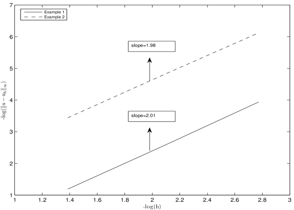
Figure 3. Convergence order estimate in $L^{\infty}$-norm.

Acknowledgements. The two authors gratefully acknowledge the research support of the Department of Science and Technology, Government of India through the National Programme on Differential Equations: Theory, Computation and Applications vide DST Project No.SERB/F/1279/2011-2012, and the support by Sultan Qaboos University under Grant IG/SCI/DOMS/13/02.

References

- [1] G. A. Baker, Error estimates for the finite element methods for second order hyperbolic equations, SIAM J. Numer. Anal., 13 (1976) 564-576.
- [2] G. A. Baker and V. A. Dougalis, The effect of quadrature errors on finite element approximations for second-order hyperbolic equations, SIAM J. Numer. Anal., 13 (1976) 577-598.
- [3] R. E. Bank and D. J. Rose, Some error estimates for the box method, SIAM J. Numer. Anal., 24 (1987) 777-787.
- [4] Z. Cai, On the finite volume element method, Numer. Math., 58 (1991) 713-735.
- [5] J.R. Cannon and Y. Lin, Nonclassical projection and Galerkin methods for nonlinear parabolic integro-differential equations, CALCOLO 25, 187-201 (1988).
- [6] J. R. Cannon and Y. Lin, Galerkin method and -error estimates for hyperbolic integro-differential equations, CALCOLO 26, 197-207 (1989).
- [7] S. H. Chou and Q. Li, Error estimates in , and in covolume methods for elliptic and parabolic problems: A unified approach, Math. Comp., 69 (2000) 103-120.
- [8] P. Chatzipantelidis, Finite volume methods for elliptic PDEs: A new approach, M2AN Math. Model. Numer. Anal., 36 (2002) 307-324.
- [9] P. Chatzipantelidis, R. D. Lazarov and V. Thomée, Error estimates for the finite volume element method for parabolic equations in convex polygonal domains, Numer. Methods PDE., 20 (2004) 650-674.
- [10] P. G. Ciarlet, The finite element method for elliptic problems, North Holland, Amsterdam, 1978.
- [11] T. Dupont, error estimates for Galerkin methods for second order hyperbolic equations, SIAM J. Numer. Anal., 10 (1973) 880-889.
- [12] R. E. Ewing, T. Lin and Y. Lin, On the accuracy of the finite volume element method based on piecewise linear polynomials, SIAM J. Numer. Anal., 6 (2002) 1865-1888.
- [13] R. E. Ewing, R. D. Lazarov and Y. Lin, Finite Volume Element Approximations of Nonlocal Reactive Flows in Porous Media, Numer. Methods PDE., 16 (2000) 285-311.
- [14] L. C. Evans, Partial Differential Equations, American Mathematical society, Rhode Island, 1998.
- [15] R. Emymard, T. Gallou et and R. Herbin, Finite Volume Methods, Handbook of Numerical Analysis, Vol. VII, North-Holland, Amsterdam (2000) 713-1020.
- [16] S. Kumar, N. Nataraj and A. K. Pani, Finite volume element method for second order hyperbolic equations, Int. J. Numer. Anal. Model., 5 (2008), 132-151.
- [17] R. H. Li, Z. Y. Chen and W. Wu, Generalized Difference Methods for Differential Equations, Marcel Dekker, New York, 2000.
- [18] Y. Lin, On maximum norm estimates for Ritz-Volterra projections and applications to some time dependent problems, J. Comp. Math., 15 (1997) 159-175.
- [19] Y. Lin, J. Lin and M. Yang, Finite volume element methods: an overview on recent developments, Int. J. Numer. Anal. Model, Series B, 4 (2013) 14-34.
- [20] Y. Lin, V. Thomée and L. B. Wahlbin, Ritz-Volterra projection onto finite element spaces and application to integro-differential and related equations, SIAM J. Numer. Anal., 28 (1991) 1047-1070.
- [21] A. K. Pani, V. Thomée, and L. B. Wahlbin, Numerical methods for hyperbolic and parabolic integro-differential equations, J. Integral Equations Appl. 4 (1992), 533–584.
- [22] J. Rauch, On convergence of the finite element method for the wave equation, SIAM J. Numer. Anal., 22 (1985) 245-249.
- [23] M. Renardy, W. Hrusa, and J. Nohel, Mathematical problems in viscoelasticity, Pitman Monographs and Survey in Pure Appl. Math. No. 35, 1987, New York, Wiley.
- [24] R. K. Sinha, Finite element approximations with quadrature for second-order hyperbolic equations, Numer. Methods PDE., 18 (2002) 537-559.
- [25] R. K. Sinha, R. E. Ewing and R. D. Lazarov, Some new error estimates of a semidiscrete finite volume element method for parabolic nonsmooth initial data, SIAM J. Numer. Anal., 43 (2006) 2320-2343.
- [26] R. K. Sinha and A. K. Pani, The effect of spatial quadrature on finite element Galerkin approximation to hyperbolic integro-differential equations, Numer. Funct. Anal. and Optimz., 19 (1998) 1129-1153.