A Unifying Framework for Typical Multi-Task Multiple Kernel Learning Problems

Abstract

Over the past few years, MKL (MKL) has received significant attention among data-driven feature selection techniques in the context of kernel-based learning. MKL formulations have been devised and solved for a broad spectrum of machine learning problems, including MTL (MTL). Solving different MKL formulations usually involves designing algorithms that are tailored to the problem at hand, which is, typically, a non-trivial accomplishment.

In this paper we present a general MT-MKL (MT-MKL) framework that subsumes well-known MT-MKL formulations, as well as several important MKL approaches on single-task problems. We then derive a simple algorithm that can solve the unifying framework. To demonstrate the flexibility of the proposed framework, we formulate a new learning problem, namely PSCS (PSCS) MT-MKL, and demonstrate its merits through experimentation.

Keywords: Multiple Kernel Learning, Multi-task Learning, Support Vector Machines

1 Introduction

Kernel methods play an important role in machine learning due to their elegant property of implicitly mapping samples from the original space into a potentially infinite-dimensional feature space, in which inner products can be calculated directly via a kernel function. It is desired that samples are appropriately distributed in the feature space, such that kernel-based models, like SVM[4] [20], could perform better in the feature space than in the original space. Since the feature space is implicitly defined via the kernel function, it is important to choose the kernel appropriately for a given task. In recent years, substantial effort has been devoted on how to learn such kernel function (or equivalently, kernel matrix) from the available data. According to the MKL approach [13], which is one of the most popular strategies for learning kernels, multiple predetermined kernels are, most commonly, linearly combined. Subsequently, in lieu of tuning kernel parameters via some validation scheme, the combination coefficients are adapted to yield the optimal kernel in a data-driven manner. A thorough review of MKL methods and associated algorithms is provided in [7].

So far, several MKL formulations, along with their optimization algorithms, have been proposed. The earlier work in [13] suggests a MKL formulation with trace constraints over the linearly combined kernels, which is further transformed into a solvable Semi-Definite Programming problem. Also, Simple-MKL [14] relies on a MKL formulation with $L_{1}$-norm constrained coefficients. In each iteration of the algorithm, a SVM problem is solved by taking advantage of an existing efficient SVM solver and the coefficients are updated via a gradient-based scheme. A similar algorithm is also applied in [23]. In [11], an $L_{2}$-norm constraint is applied to the linear combination coefficients and the proposed min-max formulation is transformed into a SIP (SIP) problem, which is then solved via a cutting plane algorithm. Moreover, two algorithms are proposed in [12] to solve the $L_{p}$-MKL formulation, where the coefficient constraint is generalized to an $L_{p}$-norm constraint. The relationship between the latter $L_{p}$-MKL formulation and one that entails a Group-Lasso regularizer is pointed out in [24], which utilizes a block coordinate descent algorithm to solve the problem in the primal domain. Besides MKL-based SVM models, a MKL formulation for KRR (KRR)[16] has been proposed in [3]. Cast as a min-max problem, it is solved via an interpolated iterative algorithm, which takes advantage of the closed-form solution for the KRR kernel coefficients.

Furthermore, MKL has been applied to MTL giving rise to MT-MKL approaches, where several tasks with shared feature representations are simultaneously learned. As was the case with single-task MKL approaches mentioned in the previous paragraph, most MT-MKL formulations that have appeared in the literature are accompanied by an algorithm tailored to their particular formulation. For example, a framework is formulated in [18], where individual tasks utilize their own task-specific space in conjunction with a shared space component, while the balance between these two components is controlled through weights. Subsequently, an exchange algorithm is proposed to solve the resulting min-max problem. Additionally, in [1], a Group-Lasso regularizer on SVM weights is considered that yields coefficient sparsity within a group of tasks and non-sparse regularization across groups. The resulting problem is solved in the dual domain via a mirror descent-based algorithm. Also, in [15], the Group-Lasso regularizer is generalized to $L_{p}-L_{q}$ regularization and two optimization problems are addressed, one being convex and the other non-convex. Next, for each of these two formulations, a specialized algorithm is proposed. Furthermore, in [22], MT-MKL is formulated in the primal domain by penalizing the SVM weight of each task to be close to a shared common weight. Finally, maximum entropy discrimination is employed in [9] to construct a MT-MKL framework.

Proposing useful MKL formulations and devising effective algorithms specifically tailored to solving them is, in most cases, a non-trivial task; such an endeavor requires fair amounts of insight and ingenuity. This is even more so true, when one considers applying MKL to MTL problems. In this paper, we present a general kernel-based MT-MKL framework that subsumes well-known MT-MKL formulations, as well as several important MKL approaches on single-task machine learning problems. Its unifying character stems from its applicability to prominent kernel-based tasks, such as SVM-based binary classification, KRR-based regression and outlier detection based on One-Class SVM [17] and SVDD (SVDD) [19], to name a few important ones. Also, it accommodates various feature space sharing approaches that may be encountered in a MT-MKL setting, as well as single-task MKL settings with different constraints. For example, it subsumes $L_{2}$-MKL and $L_{p}$-MKL considered in [11] and [12], the KRR-based MKL in [3] and the MT-MKL formulations in [18] and [15]. We introduce our framework in Section 2.

In Section 3 we state an equivalency between solving SIP problems and EPF (EPF) optimization, which may be viewed as a useful result on its own. As the new framework can be cast as a SIP problem, the previous equivalency allows us in Section 4 to eventually derive a straightforward and easy to implement algorithm for solving the new EPF-based formulation. For a given MT-MKL problem that is a special case of our framework, the availability of our algorithm eliminates the need of using an existing, potentially complicated, algorithm or deriving a new algorithm that is tailored to the problem at hand. A further major advantage of the algorithm is that it can leverage from already existing efficient kernel machine solvers (e.g., SVM solvers) or closed-form solutions (e.g., KRR solution) for given problems.

In Section 5, we present a new specialization of our framework, called PSCS MT-MKL. It permits some tasks to share a common feature space, while other tasks are allowed to utilize their own feature space. This approach follows the spirit of recent MTL research, which allows tasks to be grouped, while tasks belonging to the same group can share information with each other. Some examples include the works in [25], [8], [10] and [26], to name a few. This is a generalization of the traditional MTL setting, according to which all tasks are considered as one group and are learned concurrently. Our PSCS MT-MKL formulation is a combination of the grouped MTL setting and MKL, which appreciably differs from previously cited works. The new formulation concretely showcases the generality of the proposed MT-MKL framework, the flexibility in choosing a suitable MT-MKL feature sharing strategy, as well as the usefulness of the derived algorithm. The merits of PSCS are illustrated in Section 6, where we compare its performance on classification benchmark data sets against the common-space (CS) and independent-space (IS) alternatives. Proofs of our analytical work are given in the appendices.

2 Problem Formulation

Consider a supervised learning task with parameter $\boldsymbol{\alpha}$, which can be expressed in the form

$$\max_{\boldsymbol{\alpha}\in\boldsymbol{\Omega}(\boldsymbol{\alpha})}\bar{g}(\boldsymbol{\alpha},\boldsymbol{K})$$ (1)

where $\boldsymbol{K}$ is the kernel matrix of the training data set, i.e., its $(i,j)$ entry is $K(\boldsymbol{x}_{i},\boldsymbol{x}_{j})\triangleq\langle\phi(\boldsymbol{x}_{i}),\phi(\boldsymbol{x}_{j})\rangle_{\mathcal{H}}$, and $\mathcal{H}$ is the Hilbert space reproduced by the kernel function $k$. Here, $\phi$ is the feature mapping that is implied by the kernel function $k(\cdot,\cdot)$ and $\boldsymbol{x}_{i},\boldsymbol{x}_{j}\in\mathcal{X}$, where $\mathcal{X}$ is an input set. Also, suppose $\bar{g}$ has a finite maximum, a finite number of local maxima with respect to $\boldsymbol{\alpha}$ in the feasible set $\boldsymbol{\Omega}(\boldsymbol{\alpha})\subset\mathbb{R}^{n}$ and is affine with respect to the individual entries of $\boldsymbol{K}$. Some well-known supervised learning tasks that feature these characteristics are considered in SVM, KRR, SVDD and One-Class SVM. Their dual-domain objective functions $\bar{g}$ for $n$ training samples are given in Equation (2) through Equation (5) respectively.

$$\bar{g}_{\scriptscriptstyle SVM}(\boldsymbol{\alpha},\boldsymbol{K})\triangleq\boldsymbol{\alpha}^{\prime}\boldsymbol{1}-\frac{1}{2}\boldsymbol{\alpha}^{\prime}\boldsymbol{YKY}\boldsymbol{\alpha},$$ (2)

$$\text{with}\;\;\boldsymbol{\Omega}(\boldsymbol{\alpha})\triangleq\{\boldsymbol{\alpha}\in\mathbb{R}^{n}:\boldsymbol{0}\preceq\boldsymbol{\alpha}\preceq C\boldsymbol{1},\boldsymbol{\alpha}^{\prime}\boldsymbol{y}=0\}$$

$$\bar{g}_{\scriptscriptstyle KRR}(\boldsymbol{\alpha},\boldsymbol{K})\triangleq 2\boldsymbol{\alpha}^{\prime}\boldsymbol{y}-\boldsymbol{\alpha}^{\prime}(\lambda\boldsymbol{I}+\boldsymbol{K})\boldsymbol{\alpha},$$ (3)

$$\text{with}\;\;\boldsymbol{\Omega}(\boldsymbol{\alpha})\triangleq\mathbb{R}^{n}$$

$$\bar{g}_{\scriptscriptstyle SVDD}(\boldsymbol{\alpha},\boldsymbol{K})\triangleq\boldsymbol{\alpha}^{\prime}\boldsymbol{k}-\boldsymbol{\alpha}^{\prime}\boldsymbol{K}\boldsymbol{\alpha},$$ (4)

$$\text{with}\;\;\boldsymbol{\Omega}(\boldsymbol{\alpha})\triangleq\{\boldsymbol{\alpha}\in\mathbb{R}^{n}:\boldsymbol{0}\preceq\boldsymbol{\alpha}\preceq C\boldsymbol{1},\boldsymbol{\alpha}^{\prime}\boldsymbol{1}=1\}$$

$$\bar{g}_{\scriptscriptstyle OCSVM}(\boldsymbol{\alpha},\boldsymbol{K})\triangleq-\boldsymbol{\alpha}^{\prime}\boldsymbol{K\alpha},$$ (5)

$$\text{with}\;\;\boldsymbol{\Omega}(\boldsymbol{\alpha})\triangleq\{\boldsymbol{\alpha}\in\mathbb{R}^{n}:\boldsymbol{0}\preceq\boldsymbol{\alpha}\preceq\frac{1}{\nu l}\boldsymbol{1},\boldsymbol{\alpha}^{\prime}\boldsymbol{1}=1\}$$

In the above examples, $\cdot^{\prime}$ signifies transposition vector/matrix , $\boldsymbol{y}\triangleq[y_{1},\cdots,y_{n}]^{\prime}$ is the target vector, $\boldsymbol{k}\triangleq[k(\boldsymbol{x}_{1},\boldsymbol{x}_{1}),\cdots,k(\boldsymbol{x}_{n},\boldsymbol{x}_{n})]^{\prime}$ and $\boldsymbol{Y}\triangleq\mathrm{diag}(\boldsymbol{y})$, where $\mathrm{diag}(\cdot)$ is an operator yielding a diagonal matrix, whose diagonal is formed by the operand’s vector argument. Additionally, $C,\lambda,\nu,l$ are scalar non-negative regularization parameters for the corresponding learning problems and $\boldsymbol{1}$ is the all-ones vector of appropriate dimension.

Assume, now, that we have $T$ such tasks and let $\{\boldsymbol{x}_{i}^{t},y_{i}^{t}\}$, $i=1,\cdots,N_{t}$, be the training data for task $t$, where $t=1,\cdots,T$. Let $k_{m}(\boldsymbol{x}_{i}^{t},\boldsymbol{x}_{j}^{t})\triangleq\langle\phi_{m}(\boldsymbol{x}_{i}^{t}),\phi_{m}(\boldsymbol{x}_{j}^{t})\rangle_{\mathcal{H}_{m}}$, where $m=1,\cdots M$, be the $m$-th pre-specified kernel function and $\phi_{m}$ be the $m$-th associated feature mapping. Also, let $\boldsymbol{K}_{m}^{t}$ be the $N_{t}\times N_{t}$ kernel matrix of the training data corresponding to the $t$-th task and calculated using the $m$-th kernel function, i.e. $\boldsymbol{K}_{m}^{t}$ has elements $k_{m}(\boldsymbol{x}_{i}^{t},\boldsymbol{x}_{j}^{t})$, where $i,j=1,\cdots,N_{t}$. In this paper we consider the MT-MKL framework that is formulated as follows:

$$\min_{\boldsymbol{\theta}\in\boldsymbol{\Psi}(\boldsymbol{\theta})}\max_{\boldsymbol{a}\in\boldsymbol{\Omega}(\boldsymbol{a})}\sum_{t=1}^{T}\bar{g}(\boldsymbol{\alpha}^{t},\sum_{m=1}^{M}\theta_{m}^{t}\boldsymbol{K}_{m}^{t})$$ (6)

where $\boldsymbol{a}\triangleq[\boldsymbol{\alpha}^{1^{\prime}},\cdots,\boldsymbol{\alpha}^{T^{\prime}}]^{{}^{\prime}}\in\mathbb{R}^{N}$, $N=\sum_{t=1}^{T}N_{t}$, and $\boldsymbol{\alpha}^{t^{\prime}}$ denotes the transpose of $\boldsymbol{\alpha}^{t}\in\mathbb{R}^{N_{t}},t=1,\cdots,T$. Similarly, $\boldsymbol{\theta}$ stands for the vector with elements $\theta_{m}^{t}$.

The framework is able to incorporate various feature space sharing approaches by appropriately specifying the feasible region of the kernel combination coefficients $\boldsymbol{\theta}$. For example, for $T=1$ it can specialize to $L_{p}$-norm MKL [12], where $p\geq 1$, by using $\boldsymbol{\Psi}(\boldsymbol{\theta})=\{\boldsymbol{\theta}:\|\boldsymbol{\theta}\|_{p}\leq 1,\boldsymbol{\theta}\succeq\boldsymbol{0}\}$. Obviously, the $L_{2}$-norm MKL [11] is also covered by our framework. Additionally, it can express the MT-MKL model in [18] that allows individual tasks to utilize their own task-specific space in conjunction with a shared space component. This is achieved by specifying $\boldsymbol{\Psi}(\boldsymbol{\theta})=\{\boldsymbol{\theta}:\theta_{m}^{t}=\zeta_{m}+\gamma_{m}^{t},\zeta_{m}\geq 0,\gamma_{m}^{t}\geq 0,\sum_{m=1}^{M}\theta_{m}^{t}=1,$ $\sum_{m=1}^{M}\sum_{t=1}^{T}\gamma_{m}^{t}\leq\beta\}$. Hence, our framework also subsumes the Common Space (CS) and Independent Space (IS) MT-MKL models as special cases. The former is obtained by letting $\theta_{m}^{t}=\zeta_{m},\forall t,m$. In this case, all tasks share a common kernel function determined by the coefficients $\zeta_{m}$’s. Appropriate constraints can be added on $\boldsymbol{\zeta}$, such as the $L_{p}$-norm constraint. On the other hand, if we let $\boldsymbol{\theta}^{t}\triangleq[\theta_{1}^{t},\cdots,\theta_{M}^{t}]^{\prime}$ and add independent constraints on each $\boldsymbol{\theta}^{t}$, then we obtain the IS model, where each task occupies its own feature space.

To mention a final example, a Group-Lasso type regularizer is employed on the SVM primal-domain weights in [1], which leads to intricate optimization problems and algorithms. Our framework specializes to this problem by specifying $\boldsymbol{\Psi}(\boldsymbol{\theta})=\{\boldsymbol{\theta}:\boldsymbol{\theta}\succeq\boldsymbol{0},(\sum_{t=1}^{T}\|\boldsymbol{\theta}^{t}\|_{p}^{q})^{1/q}\leq a,p\geq 1,q\geq 1\}$. By appropriately choosing the values of $p$ and $q$, different level of group-wise and intra-group sparsity can be obtained. In this case too, using our framework leads to an easier formulation that can be solved in a much more straightforward fashion via our algorithm.

In the next section, we first transform Problem (6) to an equivalent SIP problem. Subsequently, we demonstrate the equivalency between general SIP problems and EPF-based problems. The latter result will allow us to cast Problem (6) as an EPF-based problem, which, as it turns out, can be easily solved.

3 Exact Penalty Function Method

In general, the min-max Problem (6) is not easy to solve. However, it can be transformed to an equivalent epigraph problem in the following SIP form:

$$\min_{\omega\in\mathbb{R},\boldsymbol{\theta}\in\boldsymbol{\Psi}(\boldsymbol{\theta})}\omega$$ (7)

$$\text{s.t.}\;\sum_{t=1}^{T}\bar{g}(\boldsymbol{\alpha}^{t},\sum_{m=1}^{M}\theta_{m}^{t}\boldsymbol{K}_{m}^{t})\leq\omega,\;\forall\boldsymbol{a}\in\boldsymbol{\Omega}(\boldsymbol{a}).$$

Before solving Problem (7), we first show an equivalence between EPF-based problems [21] and general SIP problems. This will eventually facilitate the development of an algorithm for solving Problem (7).

General SIP problem

Consider the general SIP problem

$$\min_{\boldsymbol{x}\in\mathbb{R}^{n}}f(\boldsymbol{x})$$ (8)

$$\text{s.t.}\;g(\boldsymbol{a},\boldsymbol{x})\leq 0,\;\forall\boldsymbol{a}\in\boldsymbol{\Omega}(\boldsymbol{a});$$

$$\;\;\;\;\;l_{u}(\boldsymbol{x})=0,u=1,\cdots,U;$$

$$\;\;\;\;\;r_{v}(\boldsymbol{x})\leq 0,v=1,\cdots,V.$$

with $U$ equality and $V$ inequality constraints. Now, suppose $f$, $g$, the $l_{u}$’s and $r_{v}$’s are continuously differentiable. The feasible region of $\boldsymbol{x}$ is determined by both the SIP constraint involving $g$ and the regular equality ($l_{u}$’s) and inequality ($r_{v}$’s) constraints. It is not difficult to see that Problem (7) is a special case of Problem (8) by defining $\boldsymbol{x}\triangleq[\omega,\boldsymbol{\theta}^{\prime}]^{\prime}$, $\boldsymbol{a}\triangleq[\boldsymbol{\alpha}^{1^{\prime}},\cdots,\boldsymbol{\alpha}^{T^{\prime}}]^{\prime}$, $f(\boldsymbol{x})\triangleq\omega$, $g(\boldsymbol{a},\boldsymbol{x})\triangleq\sum_{t=1}^{T}\bar{g}(\boldsymbol{\alpha}^{t},\sum_{m=1}^{M}\theta_{m}^{t}\boldsymbol{K}_{m}^{t})-\omega$, and letting the constraints $l_{u}$’s and $r_{v}$’s define $\boldsymbol{\Psi}(\boldsymbol{\theta})$.

EPF-based problem

For fixed $\boldsymbol{x}$, assume that there are $N(\boldsymbol{x})$ local maxima $\boldsymbol{a}_{i}^{*}\in\boldsymbol{\Omega}(\boldsymbol{a})$ of $g(\boldsymbol{a},\boldsymbol{x})$ that satisfy $g(\boldsymbol{a}^{*}_{i},\boldsymbol{x})\geq-\eta$ for some $\eta>0$ and $g(\boldsymbol{a}^{*}_{i},\boldsymbol{x})\neq g(\boldsymbol{a}^{*}_{j},\boldsymbol{x}),\forall\boldsymbol{a}^{*}_{i},\boldsymbol{a}^{*}_{j}\in\Omega(\boldsymbol{a})$. Denote this set of local maxima as $E(\boldsymbol{x})\triangleq\{\boldsymbol{a}_{i}^{*}\}_{i=1}^{N(\boldsymbol{x})}$, and let $I(\boldsymbol{x})\triangleq\{1,2,\ldots,N(\boldsymbol{x})\}$. Obviously, each $\boldsymbol{a}_{i}^{*}$ depends implicitly on $\boldsymbol{x}$. Thus, if the Implicit Function Theorem conditions hold, there is a function $\boldsymbol{a}_{i}$ of $\boldsymbol{x}$, such that $\boldsymbol{a}_{i}^{*}=\boldsymbol{a}_{i}(\boldsymbol{x})$ and we can define $h_{i}(\boldsymbol{x})\triangleq g(\boldsymbol{a}_{i}(\boldsymbol{x}),\boldsymbol{x})$. Then, the EPF $P(\boldsymbol{x})$ introduced in [21] is defined in a neighborhood of $\boldsymbol{x}$ as:

$$P(\boldsymbol{x})\triangleq f(\boldsymbol{x})+\nu\sum_{i\in I(\boldsymbol{x})}h_{i}(\boldsymbol{x})_{+}$$ (9)

where $\nu>0$ and $h_{i}(\boldsymbol{x})_{+}\triangleq\max\{0,h_{i}(\boldsymbol{x})\}$. We refer the interested reader to [21] for more details about EPF. Now, consider the EPF-based optimization problem:

$$\min_{\boldsymbol{x}\in\mathbb{R}^{n}}P(\boldsymbol{x})$$ (10)

$$\text{s.t.}\;l_{u}(\boldsymbol{x})=0,\forall u;\;r_{v}(\boldsymbol{x})\leq 0,\forall v.$$

In the next theorem, we state that the general SIP Problem (8) can be solved by solving the EPF-based Problem (10).

Theorem 1.

Let $f$, $g$, $l_{u}$’s and $r_{v}$’s in Problem (8) and Problem (10) be continuously differentiable, and let the EPF function $P(\boldsymbol{x})$ be defined as in $Equation~{}(\ref{eq:nine})$. Suppose for fixed $\boldsymbol{x}$, there are finite number of $\boldsymbol{a}_{s}\in\boldsymbol{\Omega}(\boldsymbol{a})$, $s=1,\cdots,S$, such that $g(\boldsymbol{a}_{s},\boldsymbol{x})=0$. If $\hat{\boldsymbol{x}}$ is in the feasible region of Problem (8) and solves Problem (10), then $\hat{\boldsymbol{x}}$ is a KKT (KKT) point of Problem (8).

The proof of the above theorem is given in Section .1 of the Appendix. The EPF optimization provides a way to solve the proposed general SIP-type Problem (8); in addition, it also avoids involving the SIP constraint. Obviously, since our framework of Problem (7) is a general SIP problem, we can solve its equivalent EPF-based problem instead. In the next section we introduce a simple and easy to implement algorithm to solve the EPF optimization problem for our framework.

4 Algorithm

In this section, we focus on solving the EPF-based Problem (10) for our framework. Consider Problem (10), for which we define $\boldsymbol{x}\triangleq[\omega,\boldsymbol{\theta}^{\prime}]^{\prime}$, $\boldsymbol{a}\triangleq[\boldsymbol{\alpha}^{1^{\prime}},\cdots,\boldsymbol{\alpha}^{T^{\prime}}]^{\prime}$, $f(\boldsymbol{x})\triangleq\omega$, $g(\boldsymbol{a},\boldsymbol{x})\triangleq\sum_{t=1}^{T}\bar{g}(\boldsymbol{\alpha}^{t},\sum_{m=1}^{M}\theta_{m}^{t}\boldsymbol{K}_{m}^{t})-\omega$, and let the constraints $l_{u}$’s and $r_{v}$’s define $\boldsymbol{\Psi}(\boldsymbol{\theta})$. In order to solve Problem (10), a descent algorithm is suggested in [21]. During iteration $k$ and given $\boldsymbol{x}_{k}$, $E(\boldsymbol{x}_{k})$ is calculated, a descent direction $\boldsymbol{d}_{k}$ is found, and the variables are updated as $\boldsymbol{x}_{k+1}=\boldsymbol{x}_{k}+\epsilon\boldsymbol{d}_{k}$. We remind the reader that the set $E(\boldsymbol{x})$ contains $\boldsymbol{a}_{i}^{*}$’s, which satisfy $g(\boldsymbol{a}_{i}^{*},\boldsymbol{x})\geq-\eta$. In [21] it is proven that, for sufficiently large $\nu$ and sufficiently small step length $\epsilon>0$, the limit point of $\{\boldsymbol{x}_{k}\}$ is a KKT point of Problem (8), if the sequence $\{\boldsymbol{d}_{k}\}$ is bounded and the sequence $\{\boldsymbol{x}_{k}\}$ remains in a bounded region, in which $f$ and $g$ are doubly-differentiable functions with bounded second-order derivatives. In the next theorem, we show how to find the descent direction $\boldsymbol{d}_{k}$ for our framework given $\boldsymbol{x}_{k}$ at the $k$-th iteration.

Theorem 2.

Let $\bar{g}(\boldsymbol{\alpha},\boldsymbol{K})$ be affine with respect to the individual entries of $\boldsymbol{K}$. Suppose it has a finite maximum and a finite number of local maxima with respect to $\boldsymbol{\alpha}$ in the feasible set $\boldsymbol{\Omega}(\boldsymbol{\alpha})$. Let $l_{u}$’s and $r_{v}$’s be continuous and differentiable. Let $E(\boldsymbol{x})$ and $I(\boldsymbol{x})$ be as defined in Section 3, and $\boldsymbol{a}_{i,k}\triangleq[\boldsymbol{\alpha}_{i,k}^{1^{\prime}},\cdots,\boldsymbol{\alpha}_{i,k}^{T^{\prime}}]^{\prime}\in E(\boldsymbol{x}_{k})$, $i\in I(\boldsymbol{x}_{k})=\{1,\cdots,N(\boldsymbol{x}_{k})\}$. Consider the following $N(\boldsymbol{x}_{k})$ problems, $\forall\;i\in I(\boldsymbol{x}_{k})$:

$$\min_{\boldsymbol{\theta}}\sum_{t=1}^{T}\bar{g}(\boldsymbol{\alpha}_{i,k}^{t},\sum_{m=1}^{M}\theta_{m}^{t}\boldsymbol{K}_{m}^{t})$$ (11)

$$\text{s.t.}\;l_{u}(\boldsymbol{x})=0,\forall u;\;r_{v}(\boldsymbol{x})\leq 0,\forall v.$$

Let $\hat{\boldsymbol{\theta}}_{i}$, consisting of all elements $\hat{\theta}_{m,i}^{t}$’s, be the solution to the $i$-th problem. Also, let $i_{0}=\arg\min_{i\in I(\boldsymbol{x}_{k})}$ $\max_{j\in I(\boldsymbol{x}_{k})}\{\sum_{t=1}^{T}\bar{g}(\boldsymbol{\alpha}_{j,k}^{t},\sum_{m=1}^{M}\hat{\theta}_{m,i}^{t}\boldsymbol{K}_{m}^{t})\}$ and $\hat{\omega}$ $=\min_{i\in I(\boldsymbol{x}_{k})}\max_{j\in I(\boldsymbol{x}_{k})}\{\sum_{t=1}^{T}\bar{g}(\boldsymbol{\alpha}_{j,k}^{t},\sum_{m=1}^{M}\hat{\theta}_{m,i}^{t}\boldsymbol{K}_{m}^{t}\}$. Finally, let $\hat{\boldsymbol{x}}=[\hat{\omega},\hat{\boldsymbol{\theta}}_{i_{0}}^{\prime}]^{\prime}$. Then, $\boldsymbol{d}_{k}=\hat{\boldsymbol{x}}-\boldsymbol{x}_{k}$ is a descent direction for the EPF-based Problem (10) when $\nu>1$.

The proof of the above theorem is provided in Section .2 of the appendix. Note that, if $\bar{g}$ is concave with respect to $\boldsymbol{\alpha}$, then $N(\boldsymbol{x}_{k})=1$. Thus, we have the following corollary.

Corollary 1.

Let $\bar{g}(\boldsymbol{\alpha},\boldsymbol{K})$ be affine with respect to the individual entries of $\boldsymbol{K}$ and concave with respect to $\boldsymbol{\alpha}$. Let the $l_{u}$’s and $r_{v}$’s be continuous and differentiable. Also, let $E(\boldsymbol{x})$ and $I(\boldsymbol{x})$ be defined as in Section 3 and $\boldsymbol{a}_{k}\triangleq[\boldsymbol{\alpha}_{k}^{1^{\prime}},\cdots,\boldsymbol{\alpha}_{k}^{T^{\prime}}]^{\prime}\in E(\boldsymbol{x}_{k})$. Consider the problem

$$\min_{\boldsymbol{\theta}}\sum_{t=1}^{T}\bar{g}(\boldsymbol{\alpha}_{k}^{t},\sum_{m=1}^{M}\theta_{m}^{t}\boldsymbol{K}_{m}^{t})$$ (12)

$$\text{s.t.}\;l_{u}(\boldsymbol{x})=0,\forall u;\;r_{v}(\boldsymbol{x})\leq 0,\forall v.$$

with solution $\hat{\boldsymbol{\theta}}$. Let $\hat{\omega}\triangleq\sum_{t=1}^{T}\bar{g}(\boldsymbol{\alpha}_{k}^{t},\sum_{m=1}^{M}\hat{\theta}_{m}^{t}\boldsymbol{K}_{m}^{t})$ and $\hat{\boldsymbol{x}}\triangleq[\hat{\omega},\hat{\boldsymbol{\theta}}^{\prime}]^{\prime}$. Then, $\boldsymbol{d}_{k}=\hat{\boldsymbol{x}}-\boldsymbol{x}_{k}$ is a descent direction for the EPF-based Problem (10) when $\nu>1$.

Based on the above discussion, we provide Algorithm 1. Note that we focus on the case, where $\bar{g}$ is concave, since it is the most common one in the context of kernel machines.

Algorithm 1 Algorithm for solving Problem (10)

  Choose $M$ kernel functions. Calculate the kernel matrices $\boldsymbol{K}_{m}^{t}$ for the $T$ tasks and the $M$ kernels. Choose $\bar{g}$ and $\boldsymbol{\Psi}\left(\theta\right)$ based on the characteristics of the problem at hand. Randomly initialize $\boldsymbol{\theta}_{0}\succeq\boldsymbol{0}$. Initialize $\eta$ and $\epsilon_{0}$ to small positive values. $k\leftarrow 0$.

  while not converged do

     $\boldsymbol{a}_{k}\leftarrow\arg\max_{\boldsymbol{a}\in\boldsymbol{\Omega(\boldsymbol{a})}}\sum_{t}\bar{g}(\boldsymbol{\alpha}^{t},\sum_{m}\theta_{m,k}^{t}\boldsymbol{K}_{m}^{t})$

     $\hat{\boldsymbol{\theta}}_{k}\leftarrow$ solve Problem (12) given $\boldsymbol{a}_{k}$

     $\hat{\omega}_{k}\leftarrow\sum_{t}\bar{g}(\boldsymbol{\alpha}_{k}^{t},\sum_{m}\hat{\theta}_{m,k}^{t}\boldsymbol{K}_{m}^{t})$

     $\boldsymbol{\theta}_{k+1}\leftarrow\boldsymbol{\theta}_{k}+\epsilon_{k}(\hat{\boldsymbol{\theta}}_{k}-\boldsymbol{\theta}_{k})$

     $\omega_{k+1}\leftarrow\omega_{k}+\epsilon_{k}(\hat{\omega}_{k}-\omega_{k})$

     $k\leftarrow k+1$

  end while

There are several ways to choose the step length $\epsilon_{k}$ in each step $k$. As suggested in [21], one possibility is to choose $\epsilon_{k}$ as the largest element of the set $\{1,\beta,\beta^{2},\cdots\}$, for some $\beta$, $0<\beta<1$, such that

$$[P(\boldsymbol{x}_{k}+\epsilon_{k}\boldsymbol{d}_{k})-P(\boldsymbol{x}_{k})]/\epsilon_{k}G_{k}\geq\sigma$$ (13)

where $P$ is the EPF given in Problem (10), $\sigma$ is some constant that satisfies $0<\sigma<1$, and $G_{k}$ is the directional derivative of $P$ with respect to $\boldsymbol{x}$ at the $k$-th step. It is not difficult to show that

$$G_{k}=f(\hat{\boldsymbol{x}}_{k})+\nu\;g(\boldsymbol{a}_{k},\hat{\boldsymbol{x}}_{k})_{+}-f(\boldsymbol{x}_{k})-\nu\;g(\boldsymbol{a}_{k},\boldsymbol{x}_{k})_{+}$$ (14)

where $\hat{\boldsymbol{x}}_{k}=[\hat{\omega}_{k},\hat{\boldsymbol{\theta}}^{\prime}_{k}]^{\prime}$ and $\boldsymbol{x}_{k}=[\omega_{k},\boldsymbol{\theta}^{\prime}_{k}]$. For details of $G_{k}$’s calculation, when $\bar{g}$ is not concave with respect to $\boldsymbol{\alpha}$, we refer the reader to Section .2 of the Appendix.

4.1 Analysis

The advantages of our algorithm are multifold. First, the framework hinges on relatively few mild constraints that are typically met in practice. Specifically, we only assumed that $\bar{g}$ is continuous and doubly differentiable with respect to $\boldsymbol{\alpha}$ with bounded second-order derivatives and finite number of local maxima, whose value are also finite, and $\bar{g}$ is affine with respect to the elements of $\boldsymbol{K}$. There is no need for $\bar{g}$ to be concave with respect to $\boldsymbol{\alpha}$. Note also that all these constraints are met for the $4$ examples given in Problems 2 through 5. Therefore, the framework and its associated algorithm may enjoy wide applicability.

Secondly, the maximization problem with respect to $\boldsymbol{a}$ in the first step of the algorithm can be separated into $T$ independent problems under the commonly-encountered setting, where the feasible regions of the $\boldsymbol{\alpha}^{t}$’s are mutually independent, such as in the formulations of [18] and [15]. Furthermore, in most situations, solving each of the $T$ problems can be addressed via readily-available efficient optimizers; for example, in the case of SVM problems, one could use LIBSVM [2]. In some other cases, a closed-form solution could be used instead, whenever available, such as in the case of KRR.

Thirdly, the minimization problem (12) is easy to solve. Since $\bar{g}$ is affine with respect to the individual entries of the kernel matrix, it is also affine in the entries of $\boldsymbol{\theta}$, which leads to the following optimization problem:

$$\min_{\boldsymbol{\theta}}\boldsymbol{c}^{\prime}\boldsymbol{\theta}$$ (15)

$$\text{s.t.}\;l_{u}(\boldsymbol{x})=0,\forall u;\;r_{v}(\boldsymbol{x})\leq 0,\forall v.$$

where $\boldsymbol{c}$ is a coefficient vector. For many practical models, the feasible regions of Problem (15) are such that a closed-form solution can be found. For example, in the case of an $L_{p}$-norm constrained (single-task) MKL model, the feasible region is defined by the constraints $\|\boldsymbol{\theta}\|_{p}\leq 1,\boldsymbol{\theta}\succeq\boldsymbol{0}$, for which a closed-form solution can be found. Another example is the setting considered in [18], which is of the form of Problem (12) and becomes

$$\min_{\boldsymbol{\theta}}\boldsymbol{c}^{\prime}\boldsymbol{\theta}$$ (16)

$$\text{s.t.}\;\theta_{m}^{t}=\zeta_{m}+\gamma_{m}^{t},\zeta_{m}\geq 0,\;\gamma_{m}^{t}\geq 0,\forall m,t;$$

$$\;\;\;\;\;\sum_{m=1}^{M}\theta_{m}^{t}=1,\;\forall t;\;\sum_{m=1}^{M}\sum_{t=1}^{T}\gamma_{m}^{t}\leq\beta.$$

Regarding the just-stated problem, a block coordinate descent algorithm can be employed to optimize $\boldsymbol{\zeta}=[\zeta_{1},\cdots,\zeta_{M}]$ and $\boldsymbol{\gamma}=[{\boldsymbol{\gamma}^{1}}^{\prime},\cdots,{\boldsymbol{\gamma}^{T}}^{\prime}]^{\prime}$. Each sub-problem features a linear objective function with an $L_{1}$-norm constraint, and, hence, a closed-form solution can be found. Obviously, doing so is much simpler than relying on cutting-plane algorithms employed by the authors. Finally, a closed-form solution can be obtained for an $L_{p}-L_{q}$-norm constraint as well. Proposition 1 offers closed-form solutions for problems featuring a linear objective with a $L_{p}$-norm or a $L_{p}-L_{q}$-norm constraint.

Proposition 1.

Let $\boldsymbol{c}\triangleq[c_{1},\cdots,c_{n}]^{\prime}\in\mathbb{R}^{n}$ be the concatenation of $T$ vectors $\boldsymbol{c}^{1}\in\mathbb{R}^{n_{1}},\cdots,\boldsymbol{c}^{T}\in\mathbb{R}^{n_{T}}$ with $\sum_{t=1}^{T}n_{t}=n$. Suppose that, for $t=1,\cdots,T$, each $\boldsymbol{c}^{t}$ has at least one negative element. Similarly, let $\boldsymbol{\theta}\triangleq[\theta_{1},\cdots,\theta_{n}]\in\mathbb{R}^{n}$ be the concatenation of $\boldsymbol{\theta}^{1}\in\mathbb{R}^{n_{1}},\cdots,\boldsymbol{\theta}^{T}\in\mathbb{R}^{n_{T}}$. The optimization problem

$$\min_{\boldsymbol{\theta}\in\mathbb{R}^{n}} \hskip 2.84526pt\boldsymbol{c}^{\prime}\boldsymbol{\theta}$$ (17)

s.t. $$\boldsymbol{\theta}\succeq\boldsymbol{0},\;(\sum_{t=1}^{T}\|\boldsymbol{\theta}^{t}\|_{p}^{q})^{1/q}\leq a$$

has closed-form solution

$$\begin{cases}\hat{\boldsymbol{\theta}}^{t}=\frac{\sigma^{t}(\tilde{\boldsymbol{c}}^{t})^{r}}{\|\tilde{\boldsymbol{c}}^{t}\|_{r+1}^{r}},\;\forall t,&p>1,q>1\\ \hat{\boldsymbol{\theta}}^{t}=\frac{a(\tilde{\boldsymbol{c}}^{t})^{r}}{\|\tilde{\boldsymbol{c}}^{t}\|_{r+1}^{r}}[t=t_{0}],\;\forall t,&p>1,q=1\\ \hat{\boldsymbol{\theta}}=\frac{a(\boldsymbol{c}_{*})^{s}}{\|\boldsymbol{c}_{*}\|_{s+1}^{s}},&p=1,q>1\\ \hat{\boldsymbol{\theta}}=a\boldsymbol{e}_{j},&p=1,q=1\end{cases}$$ (18)

where $\sigma^{t}\triangleq\frac{a\|\tilde{\boldsymbol{c}}^{t}\|_{r+1}^{s}}{(\sum_{t=1}^{T}\|\tilde{\boldsymbol{c}}^{t}\|_{r+1}^{s+1})^{1/q}}$, $[t=t_{0}]=1$, if $t=t_{0}$, and equals $0$, if otherwise, $t_{0}\triangleq\arg\min_{t}$ $\{\|\tilde{\boldsymbol{c}}^{t}\|_{r+1}\}$, $r\triangleq\frac{1}{p-1}$, $s\triangleq\frac{1}{q-1}$, $\tilde{\boldsymbol{c}}^{t}$ is a vector with elements $[\max\{-c_{m}^{t},0\}]_{m=1}^{M}$ and $(\tilde{\boldsymbol{c}}^{t})^{r}$ denotes element-wise exponentiation of vectors. Also, $\boldsymbol{c}^{*}$ represents the concatenation of $\boldsymbol{c}_{*}^{t}\triangleq\boldsymbol{c}^{t}\circ\boldsymbol{e}^{t}_{i_{t}},t=1,\cdots,T$, where $\circ$ is element-wise multiplication of vectors and $\boldsymbol{e}_{i_{t}}^{t}\in\mathbb{R}^{n_{t}}$ is a vector, whose $i_{t}$-th entry is $1$, while the remaining are $0$, and $i_{t}\triangleq\arg\min_{i}\{c^{t}_{i}\}$. Moreover, $\boldsymbol{e}_{j}$ is an all-$0$ vector except that its $j$-th entry equals $1$, where $j\triangleq\arg\min_{i}\{c_{i}\}$. Finally, if $\;\exists\;t$ such that $\boldsymbol{c}^{t}\succeq\boldsymbol{0}$, then $\hat{\boldsymbol{\theta}}^{t}=\boldsymbol{0}$.

The proof of the above proposition is given in Section .3 of the Appendix. It is worth mentioning that, based on Proposition 1, true within-task sparsity is only achieved, when $p=1$. Similarly, true sparsity across tasks is only obtained, when $q=1$. Therefore, depending on the desired type of sparsity, different parameter settings should be applied. For example, if within-task sparsity is desired, an $L_{1}-L_{2}$ norm with $p=1$ and $q=2$ can be utilized, as discussed in [6].

For a non-concave $\bar{g}$, but one that has a finite number of local maxima with respect to $\boldsymbol{\alpha}$ given $\boldsymbol{x}_{k}$, based on Theorem 2, we only need to solve $N(\boldsymbol{x}_{k})$ problems that are similar to Problem (12), which in most cases have closed-form solutions, as stated earlier.

Based on the above analysis, it is not difficult to see that, when a closed-form solution can be found in the second step, the complexity of our algorithm in each iteration is dominated by the complexity of the solver of the first step, such as the SVM, SVDD solver, etc. The time complexity of LIBSVM for solving a SVM or SVDD problem is given in [2]. A KRR-based model, as stated earlier, can be solved in constant time. Therefore, if the second step has a closed-form solution, then the complexity of each iteration for such model is $O(1)$. Unsurprisingly, we observed in practice that our algorithm is usually slower than the special algorithms that are tailored to each specific problem type. For example, for single-task MKL with an $L_{p}$-norm constraint as discussed in [24], a block coordinate descent algorithm is used, which is equivalent to our algorithm with step length equal to 1, when our algorithm is adapted to solve this model. Thus, since our algorithm initializes the step length to be a small value, it is not a surprise that our algorithm is slower. However, if the step length of our algorithm is initialized to $1$, both of the two methods are exactly the same. Additionally, for solving the model that is proposed in [18], when $500$ samples from the USPS data set are used for training, our algorithm takes on average $9$ seconds to train the model, while the algorithm proposed in [18] takes $7$ seconds. As expected, the advantages of our algorithm, namely its simplicity in terms of implementation and its generality are offset by a somewhat reduced computational efficiency, when compared to highly specialized algorithms that are designed to solve very specific problems.

5 The Partially Shared Common Space Model

To demonstrate the flexibility of our framework and the capability of the associated algorithm, in this section we propose a PSCS (PSCS) model for MT-MKL as a novel concrete instance of our framework. As stated earlier, in MTL, several tasks sharing a common feature representation are trained simultaneously. For MT-MKL, it is a natural choice to let all tasks share a common kernel function by letting $\theta_{m}^{t}=\zeta_{m},\forall\;t$ (see Section 2). However, in practice, there may be some problems, for which sharing a common space is not the optimal choice. For example, an MTL problem may include a few complex tasks, but also some much simpler ones. In this situation, it may be difficult to find a common feature mapping so that all tasks perform well. Therefore, it is meaningful to let complex tasks to use their own task-specific space, while allowing the remaining tasks to share a common space. Motivated by this consideration, we introduce the PSCS problem formulation shown below:

$$\min_{\boldsymbol{\theta},\boldsymbol{\zeta},\boldsymbol{\gamma}}\max_{\boldsymbol{a}\in\boldsymbol{\Omega}(\boldsymbol{a})}\sum_{t=1}^{T}\bar{g}(\boldsymbol{\alpha}^{t},\sum_{m=1}^{M}\theta_{m}^{t}\boldsymbol{K}_{m}^{t})$$ (19)

$$\text{s.t.}\;\theta_{m}^{t}=\zeta_{m}+\gamma_{m}^{t},\;\forall m,\;t;$$

$$\boldsymbol{\zeta}\succeq\boldsymbol{0},\;\|\boldsymbol{\zeta}\|_{p}\leq 1,\;p\geq 1;$$

$$\boldsymbol{\gamma}\succeq\boldsymbol{0},\;(\sum_{t=1}^{T}\|\boldsymbol{\gamma}^{t}\|_{p}^{q})^{1/q}\leq 1,\;p\geq 1,\;q\geq 1.$$

The feasible region of $\boldsymbol{\theta}$ is chosen to meet our objectives: the $L_{p}$-norm constraint controls the sparsity of the common-space coefficients $\boldsymbol{\zeta}$, while the $L_{p}-L_{q}$-norm constraint controls the within-group and group-wise sparsity. Choosing $q=1$ induces sparcity on $\boldsymbol{\gamma}$ (group-wise sparsity), which will force most tasks to share a common feature space.

Due to the complicated nature of the constraints, it is far from straightforward to devise a simple, tailored algorithm to solve the PSCS model. However, Algorithm 1 can be readily applied. In each iteration, $T$ kernel machines are first trained. Next, the minimization with respect to $\boldsymbol{\theta}$ can be accomplished via block coordinate descent to optimize $\boldsymbol{\zeta}$ as a block and $\boldsymbol{\gamma}$ as another block. In addition, the closed-form solution for $\boldsymbol{\theta}$ and $\boldsymbol{\gamma}$ can be easily determined by Proposition 1.

6 Experimental Results

In the following subsections, we experimentally evaluate our PSCS model on classification tasks. To apply our framework for classification tasks, the objective function $\bar{g}$ is specified as the dual-domain objective function for SVM training:

$$\sum_{t=1}^{T}\bar{g}(\boldsymbol{\alpha}^{t},\sum_{m=1}^{M}\theta_{m}^{t}\boldsymbol{K}_{m}^{t})=\sum_{t=1}^{T}({\boldsymbol{\alpha}^{t}}^{\prime}\boldsymbol{1}-{\boldsymbol{\alpha}^{t}}^{\prime}\boldsymbol{Y}^{t}(\sum_{m=1}^{M}\theta_{m}^{t}\boldsymbol{K}_{m}^{t})\boldsymbol{Y}^{t}\boldsymbol{\alpha}^{t})$$ (20)

Note that all kernel functions in our experiments are used in their normalized form as $\frac{k(\boldsymbol{x},\boldsymbol{y})}{\sqrt{k(\boldsymbol{x},\boldsymbol{x})k(\boldsymbol{y},\boldsymbol{y})}}$.

6.1 A qualitative case study

To qualitatively illustrate the potential of our framework, in this subsection we apply our approach to the well-known Iris Flower classification problem, which we will recast as a MTL problem. The associated data set includes $150$ patterns, each of which comes from one of three Iris flower classes: Setosa, Versicolour and Virginica (respectively, class $1$, $2$ and $3$). Each of these $3$ classes is represented by $50$ samples and every sample has $4$ attributes corresponding to the width and length of the flower’s sepal and pedal. We chose only two attributes, namely the sepal width and length, to form a $2$-dimensional data set, such that the distribution of patterns and the resulting decision boundaries can be visualized. Note that each attribute is normalized to $[0,1]$. We split the three-class problem into three binary classification tasks by employing a one-against-one strategy. Specifically, these are: task $1$ (class $1$ vs. class $2$), task $2$ (class $1$ vs. class $3$), task $3$ (class $2$ vs. class $3$). The data sets of task $1$ and $2$ are linearly separable, so it is desirable to obtain classifiers which will produce linear or almost-linear decision boundaries. On the other hand, the data set of task $3$ is not linearly separable. Intuitively, one would expect a reasonable solution to have tasks $1$ and $2$ share a common feature space, while allowing task $3$ to be mapped into an alternative, task-specific feature space.

For the purpose of this experiment, we employed Linear kernels, Polynomial kernels of degree $2$, and Gaussian kernels using a spread parameter value of $5$. All $150$ patterns were used for training. The $p$ parameter was set to $2$ for non-sparse kernel combination, because we want to see how different tasks affect the weights of each kernel function. Additionally, $q$ is set to $1$, because we want to achieve inter-task sparsity for $\boldsymbol{\gamma}$, i.e. some tasks share a common space specified by $\boldsymbol{\zeta}$. The experimental results are shown in Table 1 and Figure 1.

Table 1: Learned coefficients for the Iris classification multi-task problem

Kernel	$\boldsymbol{\zeta}$	$\boldsymbol{\gamma}^{1}$	$\boldsymbol{\gamma}^{2}$	$\boldsymbol{\gamma}^{3}$
Linear	0.1828	0	0	0.0295
Polynomial	0.9421	0	0	0.1976
Gaussian	0.2812	0	0	0.9333

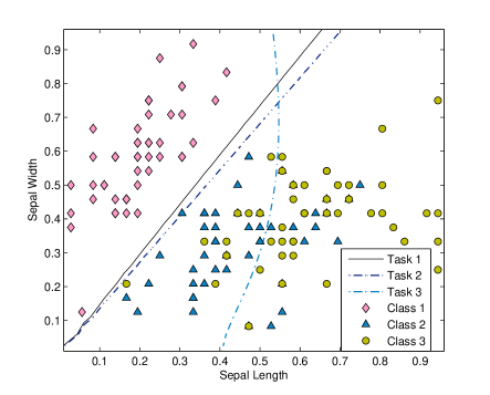
Figure 1: Decision boundaries of Iris classification multi-task problem.

It can be seen in Table 1 that all three elements in $\boldsymbol{\gamma}^{1}$ and $\boldsymbol{\gamma}^{2}$ are zero. This means that task $1$ and $2$ share a common space, which is specified by $\boldsymbol{\zeta}=[0.1828,0.9421,0.2812]$. Obviously, in the common space, the combination of Linear and Polynomial kernels has a large weight, while the Gaussian kernel plays an insignificant role. The reason behind this is that the data for tasks $1$ and $2$ are both linearly separable, so the SVM can easily find effective boundaries in the original space and the feature space implied by the Polynomial kernel. Also, we can observe that the polynomial kernel has larger weight than the linear kernel. This is because the data in the feature space induced by the polynomial kernel offers a larger margin than in the case of the original space. Note that, even though the polynomial kernel does not imply a linear feature map, the decision boundary is almost a straight line. This implies that the mapping corresponding to the polynomial kernel is almost linear in this particular case. Unlike tasks $1$ and $2$, we can see from the table that the task-specific feature space for task $3$ has a large weight corresponding to the Gaussian kernel. This is because the data for task $3$ are not linearly separable, and therefore it is difficult for the associated SVM to find a good decision boundary in the original space and the feature space implied by the Polynomial kernel. A large weight corresponding to the Gaussian kernel implies that the classifier was able to find a better decision boundary in its associated infinite-dimensional feature space. The relevant decision boundaries can be seen in Figure 1. As expected, the decision boundaries for tasks $1$ and $2$ are almost linear, while task $3$ features a non-linear decision boundary.

6.2 Quantitative Analysis on Benchmark Problems

In this subsection we first evaluate our SVM-based PSCS method using $6$ benchmark multi-class data sets obtained from the UCI repository [5]. Each associated recognition problem was cast as a multi-task classification problem by using the one-against-all approach. This is an effective method to test multi-task models; for example, refer to [9] and [26]. More specifically, we used the USPS Handwritten Digit (USPS), MNIST Handwritten Digit (MNIST), Wall-Following Robot Navigation (Robot), Statlog Shuttle (Shuttle), Statlog Vehicle Silhouettes (Vehicle), and Letter Recognition (Letter) data sets. For each data set, each class is represented by an equal number of samples. An exception is the original Shuttle data set that has seven classes, four of which are very poorly represented; for this data set we only chose data from the other three classes. Finally, for the Letter data set, we only chose the first $10$ classes to avoid handling a large number tasks.

For all experiments, the kernel and algorithm parameter settings were held fixed. Twenty experiments were conducted for each setting and the average correct classification accuracy was recorded. Linear, Polynomial, and Gaussian kernels with spread parameter values $\left\{2^{0},2^{1},2^{2},2^{3},2^{4},2^{5},2^{6},2^{7}\right\}$ were used. Regarding $p$, we held it fixed to $1.1$, as we were not concerned with obtaining within-group sparsity. Cross-validation was employed to choose values for parameters $C$ and $q$. We allowed $C$ to vary over $\left\{1/27,1/9,1/3,1,3,9,27\right\}$ and $q$ ranged from $1.0$ to $2.0$ with a step size of $0.1$. We did not consider the case, where $q>2$, since these values would yield a non-sparse group-wise $\boldsymbol{\gamma}$ vector, which was not deemed desirable.

The PSCS model was compared to the CS and IS methods, which have been described in Section 2. The experimental settings for the CS and IS methods were exactly the same as the settings used for PSCS, except that there was no parameter $q$ to be tuned for them. We considered training set sizes of $2$%, $5$%, $20$% and $50$% of the original data set to study the effect of training set size on classification accuracy. The rest of the data were split in half to form validation and test sets.

We report the experimental results (average classification accuracy of $20$ runs over randomly sampled training set) in Table 2, where the best performance is highlighted in boldface. To test the statistical significance of the differences between the best performing method and the rest, we employed a t-test to compare mean accuracies using a significance level of $\alpha=0.05$. Furthermore, we use two superscripts for each PSCS-related result to convey information about statistically significant differences in performance. The first sign refers to the comparison of PSCS to CS and the second one to the comparison to IS. A ‘$+$’ sign means that the PSCS performance is significantly better, and a ‘$=$’ sign indicates that there is no statistically significant difference.

Table 2: Experimental comparison of PSCS to the CS, IS methods on six benchmark data sets in terms of percent correct classification accuracy.

Robot	2%	5%	20%	50%
PSCS	$\textbf{75.58}^{++}$	$\textbf{82.21}^{++}$	$\textbf{90.02}^{++}$	$\textbf{92.27}^{==}$
CS	73.01	78.76	88.49	91.49
IS	73.09	78.91	87.86	91.76
Vehicle	2%	5%	20%	50%
PSCS	$\textbf{51.25}^{==}$	$\textbf{64.42}^{++}$	$\textbf{76.05}^{=+}$	$\textbf{82.35}^{++}$
CS	48.78	61.24	75.58	81.47
IS	48.62	61.76	75.04	80.62
USPS	2%	5%	20%	50%
PSCS	$\textbf{52.78}^{++}$	$\textbf{68.41}^{=+}$	$87.03^{==}$	$\textbf{93.34}^{==}$
CS	50.11	68.39	87.36	92.99
IS	46.52	63.95	86.91	92.78
Shuttle	2%	5%	20%	50%
PSCS	$\textbf{93.63}^{++}$	$\textbf{93.91}^{++}$	$\textbf{94.90}^{++}$	$\textbf{94.93}^{==}$
CS	91.80	91.84	94.20	94.90
IS	92.46	92.53	94.15	94.66
Letter	2%	5%	20%	50%
PSCS	$50.19^{==}$	$\textbf{67.43}^{++}$	$82.65^{==}$	$\textbf{89.23}^{==}$
CS	48.82	63.90	82.48	89.12
IS	51.35	64.21	82.99	89.16
MNIST	2%	5%	20%	50%
PSCS	$55.15^{=+}$	$\textbf{70.59}^{=+}$	$84.38^{==}$	$89.92^{==}$
CS	55.32	69.18	84.84	89.81
IS	51.29	66.59	84.34	90.13

It can be seen from Table 2 that, for small training set sizes ($2$% and $5$%), the PSCS method is almost always better in terms of classification accuracy compared to the CS and IS approaches and that most of the differences are statistically significant. In other words, there are learning tasks that, in practice, may benefit from partially sharing a common feature space. Additionally, for all three methods considered, as the training set size increases to $20$% or higher, their performance tends to be similar for most data sets; PSCS seems to perform significantly better only for the Vehicle data set. It appears that, when the training set is large enough, each task independently can be trained well, while sharing a common space among tasks helps little to further enhance performance.

In what follows we compare the PSCS method to the CS and IS approaches on two widely-used multi-task classification data sets, namely the Letter and Landmine data sets. The Letter data set is a collection of handwritten words compiled by Rob Kassel of the MIT Spoken Language Systems Group. The associated MTL problem involves 8 tasks, each of which is a binary classification problem. The 8 tasks are: ‘C’ vs. ‘E’, ‘G’ vs. ‘Y’, ‘M’ vs. ‘N’, ‘A’ vs. ‘G’, ‘I’ vs. ‘J’, ‘A’ vs. ‘O’, ‘F’ vs. ‘T’ and ‘H’ vs. ‘N’. Each letter is represented by a $8\times 16$ pixel image, hence by a $128$ dimensional feature vector. The goal for this problem is to correctly recognize the letters in each task. For this data set, our intention was to compare the performance of the three models on large data sizes. Therefore, we chose $1000$ samples from each class, so that each task had $2000$ training samples. Note that, due to insufficient data for classes ‘J’, ‘H’ and ‘F’, our multi-task recognition problem considered only five of the eight tasks.

On the other hand, the Landmine data set consists of $29$ binary classification tasks. Each datum is a $9$-dimensional feature vector extracted from radar images that capture a single region, which may contain a landmine field. The $9$ features include four moment-based features, three correlation-based features, one energy ration feature and one spatial variance feature [25]. Tasks $1-15$ correspond to regions with relatively high foliage, while the other $14$ tasks correspond to regions that are bare earth or desert. The tasks entail different amounts of data, varying from $30$ to $96$ samples. The goal is to classify regions as ones containing landmine fields or not.

Table 3: Experimental comparison of PSCS to the CS, IS methods on multi-task data sets in terms of percent correct classification accuracy.

Letter	0.2%	0.5%	5%	50%
PSCS	$\textbf{59.86}^{==}$	$\textbf{67.02}^{++}$	$\textbf{88.02}^{==}$	$\textbf{94.29}^{==}$
CS	56.52	65.39	87.68	94.31
IS	56.41	63.85	87.80	94.45
Landmine	20%	30%	40%	50%
PSCS	$\textbf{69.89}^{++}$	$\textbf{73.82}^{++}$	$\textbf{75.12}^{=+}$	$\textbf{77.15}^{=+}$
CS	67.24	71.62	75.04	76.96
IS	66.34	70.91	74.30	76.41

The experimental setting for these two problems were the same as previous experiments, except that we did not use $2$% and $5$% of the Landmine data set for training, due to the small size of the data set. Instead, we started from $20$% and increased the training set size in steps of $10$%. Also, for the Letter data set, in order to show results for a wider range of training set sizes, we chose $0.2$%, $0.5$%, $5$% and $50$% of the data set for training.

The experimental results are displayed in Table 3, from which it can be observed that the experimental results are consistent with the ones obtained in the previous subsection. The PSCS method can improve the classification accuracy significantly, when the training set size is relatively small, while in the case of large training sets, the improvements are not statistically significant. In the latter situation, all three methods perform similarly.

It is also worth mentioning that, by using our proposed algorithm, all three models have the same asymptotic computation complexity. Obviously, in each iteration, all three models solve the same $T$ SVM problems followed by solving Problem (12). Obviously, the former step differs for each method; Problem (12) has a closed-form solution based on Proposition 1 for each of the models. Therefore, the computational complexity per iteration is common among them and is dominated by the complexity of solving the $T$ SVM problems.

On balance, since PSCS has no worse asymptotic runtime complexity, when compared to the IS and CS approaches, and since it offers a performance advantage in cases of sample scarcity, the use of PSCS seems much preferable over the IS and CS formulations.

7 Conclusions

In this paper, we proposed a MT-MKL framework, which is formulated as a min-max problem and which subsumes a broad class of kernel-based learning problems. We showed that our formulation can be optimized by solving an EPF optimization problem. Subsequently, we derived a simple algorithm to solve it, which, for some frequently-used learning tasks, is able to leverage from existing efficient solvers or from closed-form solutions. The availability of this algorithm eliminates the need of using existing, potentially much sophisticated, algorithms or devising algorithms that are specifically tailored to the problem at hand.

In order to illustrate the utility of this novel framework and associated algorithm, we devised the PSCS MT-MKL model as a special case of our framework, which allows some tasks to share a common feature space, while other tasks are allowed to be appropriately associated to their own task-specific feature spaces. Results obtained from experimenting with a collection of classification tasks demonstrated performance advantages of the PSCS formulation, especially in the case, where the amount of training data is limited.

.1 Proof to Theorem 1

First, note that if $\hat{\boldsymbol{x}}$ solves Problem (8), then the $\hat{\boldsymbol{a}}_{s}$’s, which satisfy $g(\hat{\boldsymbol{a}}_{s},\hat{\boldsymbol{x}})=0$ and $\hat{\boldsymbol{a}}_{s}\in\boldsymbol{\Omega}(\boldsymbol{a})$, are local maxima of $g(\boldsymbol{a},\hat{\boldsymbol{x}})$. By assumption, there is a finite number of such $\hat{\boldsymbol{a}}_{s}$’s, say, $S$, which means that the problem has only $S$ active constraints. We can therefore provide the KKT necessary conditions for $\hat{\boldsymbol{x}}$ to be a solution of Problem (8):

KKT conditions for Problem (8) Let $\hat{\boldsymbol{x}}$ be a solution of Problem (8). Then, there exist $\hat{\lambda}_{s}$, $s=0,\cdots,S$; $\hat{\rho}_{u}$, $u=1,\cdots,U$; $\hat{\mu}_{v}$, $v=1,\cdots,V$, not all zero, such that

$$\hat{\lambda}_{0}\phi_{j}(\hat{\boldsymbol{x}})+\sum_{s=1}^{S}\hat{\lambda}_{s}\psi_{j}(\hat{\boldsymbol{a}}_{s},\hat{\boldsymbol{x}})+\sum_{u=1}^{U}\hat{\rho}_{u}\tau_{u,j}(\hat{\boldsymbol{x}})+\sum_{v=1}^{V}\hat{\mu}_{v}\omega_{v,j}(\hat{\boldsymbol{x}})=0,\;j=1,\cdots,n$$ (21)

where $\phi_{j}(\hat{\boldsymbol{x}})$, $\psi_{j}(\hat{\boldsymbol{a}}_{s},\hat{\boldsymbol{x}})$, $\tau_{u,j}(\hat{\boldsymbol{x}})$, $\omega_{v,j}(\hat{\boldsymbol{x}})$ denote the quantities $\frac{\partial f(\boldsymbol{x})}{\partial x_{j}}|_{\boldsymbol{x}=\hat{\boldsymbol{x}}}$, $\frac{\partial g(\hat{\boldsymbol{a}}_{s},\boldsymbol{x})}{\partial x_{j}}|_{\boldsymbol{x}=\hat{\boldsymbol{x}}}$, $\frac{\partial l_{u}(\boldsymbol{x})}{\partial x_{j}}|_{\boldsymbol{x}=\hat{\boldsymbol{x}}}$, $\frac{\partial r_{v}(\boldsymbol{x})}{\partial x_{j}}|_{\boldsymbol{x}=\hat{\boldsymbol{x}}}$ respectively.

This is a direct extension of the KKT conditions of the following standard SIP problem provided in [21]:

$$\min_{\boldsymbol{x}\in\mathbb{R}^{n}}f(\boldsymbol{x})\;\text{s.t.}\;g(\boldsymbol{a},\boldsymbol{x})\leq 0,\;\forall\boldsymbol{a}\in\boldsymbol{\Omega}(\boldsymbol{a}).$$ (22)

Similarly, we can state the KKT conditions for the EPF-based Problem (10):

KKT conditions for Problem (10) Let $\hat{\boldsymbol{x}}$ be a solution of Problem (10). Then, there exist $\hat{\lambda}_{0}^{\prime}$ and $\hat{\lambda}_{s}^{\prime},\;s\in I(\hat{\boldsymbol{x}});\;\hat{\rho}_{u}^{\prime},\;u=1,\cdots,U;\;\hat{\mu}_{v}^{\prime},\;v=1,\cdots,V$, not all zero, such that

$$\hat{\lambda}_{0}^{\prime}\phi_{j}(\hat{\boldsymbol{x}})+\sum_{s\in I(\hat{\boldsymbol{x}})}\hat{\lambda}_{s}^{\prime}\psi_{j}(\hat{\boldsymbol{a}}_{s},\hat{\boldsymbol{x}})+\sum_{u=1}^{U}\hat{\rho}_{u}^{\prime}\tau_{u,j}(\hat{\boldsymbol{x}})+\sum_{v=1}^{V}\hat{\mu}_{v}^{\prime}\omega_{v,j}(\hat{\boldsymbol{x}})=0,j=1,\cdots,n$$ (23)

In light of (21) and (23), we arrive at the conclusion.

.2 Proof to Theorem 2

Before delving into the details, we provide a sketch of the proof. The proof itself includes two major stages. In the first stage, we prove that $\boldsymbol{d}_{k}=\hat{\boldsymbol{x}}-\boldsymbol{x}_{k}$ is a descent direction, if $\hat{\boldsymbol{x}}_{k}$ is the solution to the following problem:

$$\min_{\boldsymbol{x}}f(\boldsymbol{x})+\nu\sum_{i\in I(\boldsymbol{x}_{k})}g(\boldsymbol{a}_{i,k},\boldsymbol{x})_{+}$$ (24)

$$\text{s.t.}\;l_{u}(\boldsymbol{x})=0,\forall u;\;r_{v}(\boldsymbol{x})\leq 0,\forall v.$$

Note that since $\boldsymbol{x}_{k}$ is given in the $k$-th iteration and, therefore, is fixed, $I(\boldsymbol{x}_{k})$ and the $\boldsymbol{a}_{i,k}$’s are also fixed. In the second stage, we prove that the $\hat{\boldsymbol{x}}$ described in the theorem is a solution to Problem (24), when $\nu>1$.

Stage 1. We need to prove that the directional derivative of the objective function of Problem (24) is negative, given the direction $\boldsymbol{d}_{k}=\hat{\boldsymbol{x}}-\boldsymbol{x}_{k}$. Since we only consider $\bar{g}$ to be affine in the individual entries of the kernel matrix, $g(\boldsymbol{a}_{i,k},\boldsymbol{x}_{k})$ could be expressed as

$$g(\boldsymbol{a}_{i,k},\boldsymbol{x}_{k})=\sum_{t=1}^{T}[\sum_{m=1}^{M}\theta_{m,k}^{t}(\boldsymbol{b}_{1}^{t}(\boldsymbol{a}_{i,k})^{{}^{\prime}}\hat{\boldsymbol{K}}_{m}^{t}+b_{2}^{t}(\boldsymbol{a}_{i,k}))]-\omega_{k}$$ (25)

where $\boldsymbol{b}_{1}^{t}(\cdot)$ is a vector-valued function, $b_{2}^{t}(\cdot)$ is a scalar function and $\hat{\boldsymbol{K}}_{m}^{t}$ is a vector with elements $k_{m}(\boldsymbol{x}_{i}^{t},\boldsymbol{x}_{j}^{t}),$ $i,j=1,\cdots,N_{t}$. If we define $I_{+}(\boldsymbol{x})$ $\triangleq\{i\in I(\boldsymbol{x}),$ $g(\boldsymbol{a}_{i},\boldsymbol{x})>0\}$, $I_{0}(\boldsymbol{x})$ $\triangleq\{i\in I(\boldsymbol{x}),g(\boldsymbol{a}_{i},\boldsymbol{x})=0\}$, $I_{-}(\boldsymbol{x})$ $\triangleq\{i\in I(\boldsymbol{x}),g(\boldsymbol{a}_{i},\boldsymbol{x})<0\}$, then the directional derivative can be calculated as

$$G(\boldsymbol{x}_{k},\boldsymbol{d}_{k},\nu)=\boldsymbol{d}_{k}^{{}^{\prime}}\phi(\boldsymbol{x}_{k})+\nu\sum_{i\in I_{0}(\boldsymbol{x}_{k})}[\boldsymbol{d}_{k}^{{}^{\prime}}\psi(\boldsymbol{a}_{i,k},\boldsymbol{x}_{k})]_{+}+\nu\sum_{i\in I_{+}(\boldsymbol{x}_{k})}\boldsymbol{d}_{k}^{{}^{\prime}}\psi(\boldsymbol{a}_{i,k},\boldsymbol{x}_{k})$$ (26)

Let $\boldsymbol{d}_{k}\triangleq\hat{\boldsymbol{x}}-\boldsymbol{x}_{k}$, $H_{i,m,k}^{t}\triangleq\boldsymbol{b}_{1}^{t}(\boldsymbol{a}_{i,k})^{{}^{\prime}}\hat{\boldsymbol{K}}_{m}^{t}+b_{2}^{t}(\boldsymbol{a}_{i,k})$ and $\boldsymbol{H}_{i,k}$ be the vector with elements $H_{i,m,k}^{t}$, $m=1,\cdots,M$, $t=1,\cdots,T$. Then, we obtain

$$G(\boldsymbol{x}_{k},\boldsymbol{d}_{k},\nu)=(\hat{\omega}-\omega_{k})$$ (27)

$$+\nu\sum_{i\in I_{0}(\boldsymbol{x}_{k})}[\hat{\boldsymbol{\theta}}^{{}^{\prime}}\boldsymbol{H}_{i,k}-\hat{\omega}-\boldsymbol{\theta}_{k}^{{}^{\prime}}\boldsymbol{H}_{i,k}+\omega_{k}]_{+}$$

$$+\nu\sum_{i\in I_{+}(\boldsymbol{x}_{k})}(\hat{\boldsymbol{\theta}}^{{}^{\prime}}\boldsymbol{H}_{i,k}-\hat{\omega}-\boldsymbol{\theta}_{k}^{{}^{\prime}}\boldsymbol{H}_{i,k}+\omega_{k})$$

Note that $\boldsymbol{\theta}_{k}^{{}^{\prime}}\boldsymbol{H}_{i,k}-\omega_{k}=g(\boldsymbol{a}_{i,k},\boldsymbol{x}_{k})=0$, when $i\in I_{0}(\boldsymbol{x}_{k})$. Then, we get

$$G(\boldsymbol{x}_{k},\boldsymbol{d}_{k},\nu)=f(\hat{\boldsymbol{x}})+\nu\sum_{i\in I(\boldsymbol{x}_{k})}g(\boldsymbol{a}_{i,k},\hat{\boldsymbol{x}})_{+}-f(\boldsymbol{x}_{k})-\nu\sum_{i\in I(\boldsymbol{x}_{k})}g(\boldsymbol{a}_{i,k},\boldsymbol{x}_{k})_{+}$$ (28)

Since $\hat{\boldsymbol{x}}$ minimizes (24), we have that $G(\boldsymbol{x}_{k},\boldsymbol{d}_{k},\nu)\leq 0$.

Stage 2. Denote the objective function in (24) as

$$F(\omega,\boldsymbol{\theta})=F(\boldsymbol{x})=f(\boldsymbol{x})+\nu\sum_{i\in I(\boldsymbol{x}_{k})}g(\boldsymbol{a}_{i,k},\boldsymbol{x})_{+}$$ (29)

We first prove that in Problem (24), for $\nu>1$ and fixed $\boldsymbol{\theta}$, the optimal solution to $\omega$ is $\hat{\omega}=\max_{i\in I(\boldsymbol{x}_{k})}$ $\sum_{t=1}^{T}\bar{g}(\boldsymbol{\alpha}_{i,k}^{t},\sum_{m=1}^{M}\theta_{m}^{t}\boldsymbol{K}_{m}^{t})$, which yields $F(\hat{\omega},\boldsymbol{\theta})=\hat{\omega}$. To see that this is true, first consider another $\bar{\omega}>\hat{\omega}$, which implies that $F(\bar{\omega},\boldsymbol{\theta})=\bar{\omega}>\hat{\omega}$. On the other hand, if we consider $\bar{\omega}<\hat{\omega}$, then we have that

$$F(\hat{\omega},\boldsymbol{\theta})-F(\bar{\omega},\boldsymbol{\theta})=\hat{\omega}-\bar{\omega}-\nu\sum_{i\in I(\boldsymbol{x}_{k})}(\sum_{t=1}^{T}\bar{g}(\boldsymbol{\alpha}_{i,k}^{t},\sum_{m=1}^{M}\theta_{m}^{t}\boldsymbol{K}_{m}^{t})-\bar{\omega})_{+}$$ (30)

For simplicity, assume $\bar{\omega}$ is such that only one element in the summation over $i$ not zero. Then,

$$F(\hat{\omega},\boldsymbol{\theta})-F(\bar{\omega},\boldsymbol{\theta})=\hat{\omega}-\bar{\omega}-\nu(\hat{\omega}-\bar{\omega})$$ (31)

Since $\nu>1$, the above quantity is negative, which implies that $F(\hat{\omega},\boldsymbol{\theta})<F(\bar{\omega},\boldsymbol{\theta})$. When $\bar{\omega}$ is such that more elements in the summation over $i$ are not zero, the rationale is similar. Therefore, we proved that for fixed $\boldsymbol{\theta}$, the previously defined $\hat{\omega}$ is the optimum.

Based on the just-stated fact, in order to minimize $F(\omega,\boldsymbol{\theta})$, we need to find a $\boldsymbol{\theta}$ such that $\max_{i\in I(\boldsymbol{x})}$ $\sum_{t=1}^{T}\bar{g}(\boldsymbol{\alpha}_{i}^{t},\sum_{m=1}^{M}\theta_{m}^{t}\boldsymbol{K}_{m}^{t})$ is minimized:

$$\min_{\boldsymbol{\theta}}\max_{i\in I(\boldsymbol{x}_{k})}\sum_{t=1}^{T}\bar{g}(\boldsymbol{\alpha}_{i,k}^{t},\sum_{m=1}^{M}\theta_{m}^{t}\boldsymbol{K}_{m}^{t})$$ (32)

This problem is equivalent to the following:

$$\min_{\boldsymbol{\theta}}\lambda$$ (33)

$$\text{s.t.}\sum_{t=1}^{T}\bar{g}(\boldsymbol{\alpha}_{i,k}^{t},\sum_{m=1}^{M}\theta_{m}^{t}\boldsymbol{K}_{m}^{t})\leq\lambda,\forall i\in I(\boldsymbol{x}_{k}).$$

Therefore, we only need to solve the $\left|I_{k}\right|$ problems $\boldsymbol{\hat{\theta}}_{i}=\arg\min_{\boldsymbol{\theta}}\sum_{t=1}^{T}\bar{g}(\boldsymbol{\alpha}_{i,k}^{t},\sum_{m=1}^{M}\theta_{m}^{t}\boldsymbol{K}_{m}^{t}),\forall i\in I(\boldsymbol{x}_{k})$, and find a value, say $\boldsymbol{\hat{\theta}}_{i_{0}}$, that minimizes the quantity $\max_{j\in I(\boldsymbol{x}_{k})}\{\sum_{t=1}^{T}\bar{g}(\boldsymbol{\alpha}_{j,k}^{t},\sum_{m=1}^{M}\hat{\theta}_{m,i_{0}}^{t}\boldsymbol{K}_{m}^{t})\}$.

.3 Proof to Proposition 1

The results for $p=1,q=1$ and $\boldsymbol{c}^{t}\succeq\boldsymbol{0}$ are obvious. In what follows, we assume that there is at least one negative element in each $\boldsymbol{c}^{t}$. We first prove the result for $p>1,q>1$. In this situation, the problem can be written as

$$\min_{\boldsymbol{\theta}\in\mathbb{R}^{n},\boldsymbol{\sigma}\in\mathbb{R}^{T}} \hskip 2.84526pt\boldsymbol{c}^{\prime}\boldsymbol{\theta}$$ (34)

s.t. $$\boldsymbol{\theta}\succeq\boldsymbol{0},\;\|\boldsymbol{\theta}^{t}\|_{p}=\sigma^{t},\;\forall\;t;\|\boldsymbol{\sigma}\|_{q}\leq a.$$

Note that the above problem is equivalent to the following:

$$\min_{\boldsymbol{\theta}\in\mathbb{R}^{n},\boldsymbol{\sigma}\in\mathbb{R}^{T}} \hskip 2.84526pt\boldsymbol{c}^{\prime}\boldsymbol{\theta}$$ (35)

s.t. $$\boldsymbol{\theta}\succeq\boldsymbol{0},\;\|\boldsymbol{\theta}^{t}\|_{p}\leq\sigma^{t},\;\forall\;t;\|\boldsymbol{\sigma}\|_{q}\leq a.$$

since the optimum $\boldsymbol{\theta}^{t}$ for the previously-stated problem must occur on the boundary. The Lagrangian of Problem (35) takes the form of

$$L=\sum_{t=1}^{T}(\boldsymbol{c}^{t^{\prime}}\boldsymbol{\theta}^{t}+\alpha^{t}(\|\boldsymbol{\theta}^{t}\|_{p}-\sigma^{t})-\boldsymbol{\beta}^{t^{\prime}}\boldsymbol{\theta}^{t})+\gamma(\|\boldsymbol{\sigma}\|_{q}-1)$$ (36)

where $\alpha$ and $\boldsymbol{\beta}$ are the Lagrangian multipliers corresponding to the inequality constraints. Setting its partial derivatives with respect to $\boldsymbol{\theta}^{t}$ and $\boldsymbol{\sigma}$ to $\boldsymbol{0}$ and adding the complementary slackness conditions yields the following set of equalities:

$$\left\{\begin{array}[]{l}\boldsymbol{c}^{t}+\alpha^{t}\|\boldsymbol{\theta}^{t}\|_{p}^{1-p}(\boldsymbol{\theta}^{t})^{p-1}-\boldsymbol{\beta}^{t}=\boldsymbol{0};\;\forall t\\ \gamma\|\boldsymbol{\sigma}\|_{q}^{1-q}\boldsymbol{\sigma}^{q-1}-\boldsymbol{\alpha}=\boldsymbol{0};\\ \alpha^{t}(\|\boldsymbol{\theta}^{t}\|_{p}-\sigma^{t})=0;\;\forall t\\ \beta_{m}^{t}\theta_{m}^{t}=0;\;\forall m,\;t\\ \gamma(\|\boldsymbol{\sigma}\|_{q}-1)=0.\end{array}\right.$$ (37)

Note that $\boldsymbol{\alpha}$ should not be $\boldsymbol{0}$, otherwise the minimum of $L$ would be either minus infinity or $0$, which are both trivial cases. Therefore, we have that

$$\left\{\begin{array}[]{l}\|\boldsymbol{\theta}^{t}\|_{p}=\sigma^{t};\;\forall t\\ \boldsymbol{\theta}^{t}=\sigma^{t}[\frac{1}{\alpha^{t}}(\boldsymbol{\beta}^{t}-\boldsymbol{c}^{t})]^{\frac{1}{p-1}}\;\forall t\end{array}\right.$$ (38)

Considering (37) and the fact that $\alpha^{t}>0$, as well as assuming that $\sigma^{t}>0$, we have $\beta_{m}(\beta_{m}^{t}-c_{m}^{t})^{\frac{1}{p-1}}=0,\;\forall m$. Since $\beta_{i}^{t}\geq 0$, we conclude that

$$\left\{\begin{matrix}\beta_{m}^{t}=0&\text{if}\;c_{m}^{t}\leq 0\\ \beta_{m}^{t}=c_{m}^{t}&\text{otherwise}.\end{matrix}\right.$$ (39)

So, if we let $\tilde{\boldsymbol{c}}^{t}\triangleq[\tilde{c}_{1}^{t},\cdots,\tilde{c}_{n}^{t}]^{\prime}$ and $\tilde{c}_{m}^{t}\triangleq\beta_{m}^{t}-c_{m}^{t}$, we obtain $\tilde{c}_{m}^{t}=\max\left\{-c_{m}^{t},0\right\},\;\forall m$. We end up with $\boldsymbol{\theta}^{t}=\sigma^{t}(\frac{\tilde{\boldsymbol{c}}^{t}}{\alpha^{t}})^{\frac{1}{p-1}}\propto(\tilde{\boldsymbol{c}}^{t})^{\frac{1}{p-1}}$. Since $\boldsymbol{\theta}^{t}$ needs to satisfy $\left\|\boldsymbol{\theta}^{t}\right\|_{p}=\sigma^{t}$, we normalize $(\tilde{\boldsymbol{c}}^{t})^{\frac{1}{p-1}}$ and get

$$\boldsymbol{\theta}^{t}=\sigma^{t}\frac{(\tilde{\boldsymbol{c}}^{t})^{\frac{1}{p-1}}}{\|\tilde{\boldsymbol{c}}^{t}\|_{\frac{p}{p-1}}^{\frac{1}{p-1}}}$$ (40)

In the previous derivation, we assumed that $\sigma^{t}\neq 0$. If $\sigma^{t}=0$, we know immediately from (38) that $\boldsymbol{\theta}^{t}=\boldsymbol{0}$. By the same rationale, we can show that $(\sigma^{t})^{q-1}\propto\alpha^{t}=\|\tilde{\boldsymbol{c}}^{t}\|_{\frac{p}{p-1}}$. Noting that the optimal $\boldsymbol{\sigma}$ must occur on the boundary, we arrive at the solution

$$\sigma^{t}=\frac{a\|\boldsymbol{c}^{t}\|_{r+1}^{s}}{(\sum_{t=1}^{T}\|\boldsymbol{c}^{t}\|_{r+1}^{s+1})^{1/q}}.$$ (41)

When $q=1$, (40) is still valid. Therefore, we substitute (40) into (35) to obtain:

$$\min_{\boldsymbol{\sigma}}\sum_{t=1}^{T}\sigma^{t}\|\tilde{\boldsymbol{c}}^{t}\|_{r+1}\;\text{s.t.}\;\boldsymbol{\sigma}>\boldsymbol{0},\;\sum_{t=1}^{t}\sigma^{t}\leq a$$ (42)

Note that the constraint $\boldsymbol{\sigma}>\boldsymbol{0}$ is added, since $\sigma^{t}=\|\boldsymbol{\theta}^{t}\|_{p}$. Obviously, the optimum $\boldsymbol{\sigma}$ is $\sigma^{t}=a[t=t_{0}]$, where $t_{0}\triangleq\arg\min_{t}\{\|\hat{\boldsymbol{c}}^{t}\|_{r+1}\}$.

When $p=1$, we first optimize with respect to $\boldsymbol{\theta}$. By fixing $\boldsymbol{\sigma}$, our problem can be split into $T$ minimization problems:

$$\min_{\boldsymbol{\theta}_{t}}(\boldsymbol{c}^{t})^{\prime}\boldsymbol{\theta}^{t}\;\;\text{s.t.}\;\boldsymbol{\theta}^{t}\succeq\boldsymbol{0},\sum_{i=1}^{N_{t}}\theta_{i}^{t}\leq\sigma^{t}$$ (43)

The solution to this problem is $\boldsymbol{\theta}^{t*}=\sigma^{t}\boldsymbol{e}_{i_{t}}^{t}$. Substituting this result into Problem (35), optimizing with respect to $\boldsymbol{\sigma}$ and using an approach similar to the previous proof yields the desired result.

References

- [1] Jonathan Aflalo, Aharon Ben-Tal, Chiranjib Bhattacharyya, Jagarlapudi Saketha Nath, and Sankaran Raman. Variable sparsity kernel learning. Journal of Machine Learning Research, 12:565–592, February 2011.
- [2] Chih-Chung Chang and Chih-Jen Lin. LIBSVM: A library for support vector machines. ACM Transactions on Intelligent Systems and Technology, 2:27:1–27:27, 2011. Software available at http://www.csie.ntu.edu.tw/~cjlin/libsvm.
- [3] Corinna Cortes, Mehryar Mohri, and Afshin Rostamizadeh. regularization for learning kernels. In UAI, 2009.
- [4] Corinna Cortes and Vladimir Vapnik. Support-vector networks. Machine Learning, 20:273–297, 1995.
- [5] A. Frank and A. Asuncion. UCI machine learning repository, 2010. Available from: http://archive.ics.uci.edu/ml.
- [6] J. Friedman, T. Hastie, and R. Tibshirani. A note on the group lasso and a sparse group lasso. ArXiv e-prints, 2010. Available from: http://arxiv.org/abs/1001.0736, arXiv:1001.0736.
- [7] Mehmet Gonen and Ethem Alpaydin. Multiple kernel learning algorithms. Journal of Machine Learning Research, 12:2211–2268, 2011.
- [8] Laurent Jacob, Francis Bach, and Jean-Philippe Vert. Clustered multi-task learning: a convex formulation. In NIPS, 2008.
- [9] Tony Jebara. Multitask sparsity via maximum entropy discrimination. Journal of Machine Learning Research, 12:75–110, 2011.
- [10] Zhuoliang Kang, Kristen Grauman, and Fei Sha. Learning with whom to share in multi-task feature learning. In ICML, 2011.
- [11] Marius Kloft, Ulf Brefeld, Pavel Laskov, and Soren Sonnenburg. Non-sparse multiple kernel learning. In NIPS Workshop on Kernel Learning: Automatic Selection of Optimal Kernels, 2008.
- [12] Marius Kloft, Ulf Brefeld, Soren Sonnenburg, Pavel Laskov, Klaus-Robert Muller, and Alexander Zien. Efficient and accurate lp-norm multiple kernel learning. In NIPS, 2009.
- [13] Gert R.G. Lanckriet, Nello Cristianini, Peter Bartlett, Laurent El Ghaoui, and Michael I. Jordan. Learning the kernel matrix with semidefinite programming. Journal of Machine Learning Research, 5:27–72, 2004.
- [14] Alain Rakotomamonjy, Francis R. Bach, Stephane Canu, and Yves Grandvalet. Simple-MKL. Journal of Machine Learning Research, 9:2491–2521, 2008.
- [15] Alain Rakotomamonjy, Remi Flamary, Gilles Gasso, and Stephane Canu. penalty for sparse linear and sparse multiple kernel multitask learning. IEEE Transactions on Neural Networks, 22:1307–1320, 2011.
- [16] Craig Saunders, Alexander Gammerman, and Volodya Vovk. Ridge regression learning algorithm in dual variables. In ICML, 1998.
- [17] Bernhard Schölkopf, John C. Platt, John Shawe-Taylor, and Alex J. Smola. Estimating the support of a high-dimensional distribution. Neural Computation, 13:1443–1471, 2001.
- [18] Lei Tang, Jianhui Chen, and Jieping Ye. On multiple kernel learning with multiple labels. In IJCAI, 2009.
- [19] David M.J. Tax and Robert P.W. Duin. Support vector domain description. Pattern Recognition Letters, 20:1191–1199, 1999.
- [20] Vladimir Vapnik. Statistical Learning Theory. Wiley-Interscience, 1998.
- [21] G. A. Watson. Globally convergent methods for semi-infinite programming. BIT Numerical Mathematics, 21:362–373, 1981.
- [22] Christian Widmer, Nora C. Toussaint, Yasemin Altun, and Gunnar Ratsch. Multi-task multiple kernel learning (MT-MKL). In NIPS 2010 Workshop: New Directions in Multiple Kernel Learning, 2010.
- [23] Xinxing Xu, I.W. Tsang, and Dong Xu. Soft margin multiple kernel learning. IEEE Transactions on Neural Networks and Learning Systems, 24:749–761, 2013.
- [24] Zenglin Xu, Rong Jin, Haiqin Yang, Irwin King, and Michael R. Lyu. Simple and efficient multiple kernel learning by group lasso. In ICML, 2010.
- [25] Ya Xue, Xuejun Liao, Laurence Carin, and Balaji Krishnapuram. Multi-task learning for classification with dirichlet process priors. Journal of Machine Learning Research, 8:35–63, 2007.
- [26] Leon Wenliang Zhong and James T. Kwok. Convex multitask learning with flexible task clusters. In ICML, 2012.