Distance determination to eight galaxies using expanding photosphere method

Abstract

Type IIP supernovae are recognized as independent extragalactic distance indicators, however, keeping in view of the diverse nature of their observed properties as well as the availability of good quality data, more and newer events need to be tested for their applicability as a reliable distance indicators. We use early photometric and spectroscopic data of eight type-IIP SNe to derive distances to their host galaxies using the expanding photosphere method (epm). For five of these, epm  is applied for the first time. In this work, we improved epm  application by using synow  estimated velocities and by semi-deconvolving the broadband filter responses while deriving color temperatures and black-body angular radii. We find that the derived epm  distances are consistent with that derived using other redshift independent methods.

1. Introduction

The hydrostatic nuclear burning phases of massive stars with initial masses greater than about 8 $M_{\odot}$ results in a onion-skin like stratification of nucleosynthesis yields as well as the unprocessed material consisting of iron core and successive zones of lighter elements up to helium and hydrogen (Arnett, 1996; José & Iliadis, 2011). It is understood that supernovae (SNe) explosions mark end stages in the life of these stars (Heger et al., 2003; Smartt, 2009), and the explosion results in collapse of iron core into a stellar mass compact object followed by shock-driven heating and expulsion of outer stellar envelope, although, the exact mechanism of explosion and the chemical yields from explosive nucleosynthesis are not fully understood (Woosley & Weaver, 1995; Janka, 2012; Burrows, 2013).

A majority of core-collapse events showing hydrogen lines in their optical spectra are classified as type II SNe (Filippenko, 1997), and their progenitors are thought to have retained enough hydrogen until the time of explosion. About ninety percent of all type II events are sub-classified as IIP (Smartt et al., 2009; Arcavi et al., 2010; Smith et al., 2011). The V-band light curve of IIP SNe are described by a fast rise (up to 10-15 days post explosion); a long plateau phase for about hundred days which is sustained by cooling down of shock-heated expanding ejecta by hydrogen recombination and then an exponential decline powered by radioactive decay of newly formed ⁵⁶Co  (Bose et al., 2013). Study of pre-supernova stars from the archival pre-explosion images proves beyond doubt that the progenitors of IIP SNe are red supergiant stars (Smartt et al., 2009; Poznanski, 2013).

Observations of type IIP SNe have been used to determine distances to their host galaxies using expanding photosphere method (epm), which is a variant of Baade-Wesselink method, developed and implemented first by Kirshner & Kwan (1974) for two SNe. The epm provides an estimate of cosmological distances, independent of extragalactic distance ladder, and offers alternative to verify results obtained using other tools e.g. SN Ia. Schmidt et al. (1992, 1994) applied epm to several IIP SNe out to 180 Mpc to constrain value of Hubble constant (H₀). Eastman et al. (1996) quantified the dilution factors of supernova atmospheres relative to black-body function and gave a firm theoretical foundation to epm. However, there have been discrepancies in the distances derived using epm, e.g. a value in the range 7 to 8 Mpc is obtained for SN 1999em (Hamuy et al., 2001; Leonard et al., 2002a; Elmhamdi et al., 2003), while a value of $11.7\pm 1.0$ Mpc is derived using Cepheids (Leonard et al., 2003). Subsequently, spectral-fitting expanding atmosphere method (seam) employing the full nlte supernova model atmosphere codes have been used to derive distances to SN 1999em (Baron et al., 2004; Dessart & Hillier, 2006) and the estimated value was found to be in fair agreement with the Cepheid distance. However, the seam is computationally intensive and it can only be applied to events having high signal-to-noise spectra at early phases. The epm need to be explored further.

Jones et al. (2009) derived epm distances to 12 IIP SNe using two sets of SN atmospheres, three filter subsets, the photospheric velocity estimated from Doppler-shifts of spectral lines and they found variation in epm distances up to 50% depending on the models and subsets used. Recently, Vinkó et al. (2012) applied epm to SNe 2005cs and 2011dh, both in M51 and both having densely sampled light-curves and spectra and they derived distance in good agreement with that in NED database. Takáts & Vinkó (2012) applied epm to 5 IIP SNe and found that photospheric velocity estimated using synow models of spectral lines are preferred.

Due to their high intrinsic luminosity, type IIP SNe have been detected out to z=0.6 and are expected to be more abundant at higher redshifts (Hopkins & Beacom, 2006). After finding a correlation between plateau luminosity and the photospheric velocity, Hamuy & Pinto (2002) first established IIP SNe as standardizable candles. This standard candle method (scm) is consistent with red supergiants as their progenitors. Using model light curves of IIP SNe, Kasen & Woosley (2009) gave a firm theoretical basis to the tight relationship between luminosity and expansion velocity, though they found a sensitivity to progenitor metallicity and mass. Olivares E. et al. (2010) applied scm to 37 nearby (z $<$ 0.06) SNe with relative distance precision of 12-14%, though they found systematic differences between distances derived using epm and scm.

The observed mid-plateau properties of type II-P SNe form a sequence from subluminous $M_{\rm V}\sim-15$ mag, low-velocity $v\sim$ 2000 $\rm{\,km\,s^{-1}}$ to bright $\sim-18$ mag, high-velocity $\sim$ 8000 $\rm{\,km\,s^{-1}}$ events (Hamuy, 2003). Recently, a spectroscopically subluminous IIP showing light curve properties similar to a normal luminosity event have also been observed, e.g. SN 2008in (Roy et al., 2011) and SN 2009js (Gandhi et al., 2013). Several bright events showing signs of circumstellar interaction have been observed, e.g. SNe 2007od (Inserra et al., 2011) and 2009bw (Inserra et al., 2012). The main factors governing the observed properties are nature and environments of progenitors. In view of diversity in the properties of IIP SNe, as well as the availability of good quality data for several events in the literature, more and newer events need to be tested for its applicability as reliable distance indicators. In this work, we extend the epm analysis to eight type IIP SNe having sufficient early time photometric and spectroscopic data to test the full applicability of epm and know the limitations and strength of the method.

The paper is organized as follows. The basic ingredients of the epm are briefly described in §2. The sample and data are given in §3. The epm analysis, sources of errors and results are presented and discussed in §4, followed by discussions on individual events and summary in §5.

2. method

The expanding photosphere method (EPM) is fundamentally a geometrical technique (Kirshner & Kwan, 1974; Schmidt et al., 1992), in which we compare the linear radii determined from the velocity of supernova expansion with that of angular radii estimated by fitting blackbody to the observed supernova fluxes at different epochs. For extragalactic supernovae, it is not possible to measure radii directly as they are seen as point sources, however, we may relate linear radius $R$ and angular radius $\theta$ as $\theta=R/D$, where $D$ is distance to the supernova. Furthermore, assuming a spherically symmetric expansion of the photosphere moving with velocity $v_{\rm ph}$ at time $t$ and neglecting other deceleration factor such as gravity and interstellar medium, we may write the above geometric relation as

$$t=D\left(\frac{\theta}{v_{\rm ph}}\right)+t_{0}$$ (1)

where $t_{0}$ is the time of explosion. We use this linear equation to determine $D$ and $t_{0}$. Given $t_{0}$, we can estimate $D$ for each value of $\theta/v_{\rm ph}$ and alternatively, the relation can also be solved to estimate unique values of $D$ and $t_{0}$. We note that for many supernovae, the later is not known with sufficient precision and the method can also be used to get an independent estimate of $t_{0}$ as well as to test the consistency of the fitted parameters.

Thus, to derive distance by epm, all we need are values of $v_{\rm ph}$ and $\theta$ at different $t$. The former is derived from low-resolution optical spectroscopic data while the later is estimated from broad-band photometric data.

2.1. Determination of $v_{\rm ph}$

The determination of expansion velocity of supernova at the photosphere $v_{\rm ph}$ at time $t$ is a non-trivial issue and several approaches have been evolved in the literature, see Takáts & Vinkó (2012) for a summary on merits and demerits of various approaches. The photosphere represents the optically thick and ionized part of the ejecta which emits most of the continuum radiation as a diluted blackbody and it is understood to be located in a thin spherical shell where electron-scattering optical depth of photons is 2/3 (Dessart & Hillier, 2005). In type IIP SNe, no single measurable spectral feature is directly connected with the true velocity of photosphere, however, during the plateau-phase, it is best represented by blue-shifted absorption components of P-Cygni profiles of Fe ii  at 4924Å, 5018Å and 5169Å. In early-phase ($t\leq$ 10-15 d) of SNe, the Fe ii  lines are either weak or absent and in such cases, the He i  5876Å  line can be used to estimate photospheric velocity with an accuracy of 2–4% (e.g. Vinkó & Takáts, 2007; Takáts & Vinkó, 2006), however at later phases ($t>$ 20 d), He i  lines disappear and Na i  D lines start to dominate in same spectral region. We can estimate velocities either by measuring Doppler-shift of the absorption minima using splot task of iraf (denoted as $v_{\rm pha}$) or by modelling the observed spectra with synow ($v_{\rm phs}$). We use both the methods in this work.

synow (Fisher et al., 1997, 1999; Branch et al., 2002) is a highly parameterized spectrum synthesis code with number of simplified assumptions: homologous expansion, spherical symmetry, line formation is purely due to resonant scattering in which the radiative transfer equations are solved by Sobolev approximation and the most important assumption is lte atmosphere with a sharp photosphere radiating like a blackbody. However, despite such simplified assumptions, the basic physics of expanding photosphere is preserved which gives rise to P-Cygni profiles for each spectral line. As a result, the underlying continuum of the synthetic spectra shall not match with observed ones because of the obvious fact that the physics of the continuum is significantly different and definitely not lte  but, the P-Cygni profiles shall be well reproduced in synthetic spectra which is directly related to the velocity of line formation layers. The synow also has the potential to reproduce line blending features in synthetic spectra, as in case of Fe ii  line, these are moderately contaminated by other ions, among which most prominent ones are Ba ii , Sc ii  and Ti ii . Takáts & Vinkó (2012) have compared the velocities determined from synow and cmfgen as the later model solves the nlte radiation-transfer equations for expanding photosphere, and it has been shown that the velocities from each of these model are very much consistent with each other.

Table 1Basic properties for supernovae and their host galaxies.

ID	Host	$v_{\rm rec}$	$t_{\rm ref}$	$E(B-V)_{\rm tot}$	$M_{\rm V}$	References
(SN)	galaxy	($\rm{\,km\,s^{-1}}$)	(JD)	(mag)	(mag)
(1)	(2)	(3)	(4)	(5)	(6)	(7)
SN 1999gi	NGC 3184	552	1518.2$\pm$3.1	0.21$\pm$0.09	-16.3	Leonard et al. (2002b)
SN 2004et	NGC 6946	45	3270.5$\pm$0.9	0.41	-17.1	Sahu et al. (2006); Takáts & Vinkó (2012)
SN 2005cs	NGC 5194	463	3549.0$\pm$1.0	0.05$\pm$0.02	-15.1	Pastorello et al. (2006, 2009); Baron et al. (2007)
SN 2006bp	NGC 3953	987	3834.5$\pm$2.0	0.40	-17.1	Immler et al. (2007); Quimby et al. (2007)
						Dessart et al. (2008)
SN 2008in	NGC 4303	1567	4825.6$\pm$2.0	0.10$\pm$0.10	-15.7	Roy et al. (2011)
SN 2009bw	UGC 2890	1155	4916.5$\pm$3.0	0.31$\pm$0.03	-16.8	Inserra et al. (2012)
SN 2009md	NGC 3389	1308	5162.0$\pm$8.0	0.10$\pm$0.05	-14.9	Fraser et al. (2011)
SN 2012aw	NGC 3351	778	6002.6$\pm$0.8	0.07$\pm$0.01	-16.7	Bose et al. (2013)

Notes : The columns are (1) identification of SN; (2) identification of supernova host-galaxy; (3) recession velocity of the galaxy used for doppler correction; (4) the reference epoch in JD since 2450000.0, these are adopted explosion epoch from corresponding literature; (5) the total reddening $E(B-V)_{\rm tot}$ towards the line-of-sight of SN; (6) appromximate absolute visual magnitude at $\sim$50 day; (7) references for $t_{ref}$, $E(B-V)_{\rm tot}$, $M_{\rm V}$, and the photometric and spectroscopic data.

2.2. Determination of $\theta$

In order to determine $\theta$ at time $t$, we assume that the supernova is radiating isotropically as a blackbody and hence accounting for the conservation of radiative energy we may write,

$$f_{\lambda}^{obs}=\theta^{2}\pi B_{\lambda}(T_{c})10^{-0.4A_{\lambda}}$$ (2)

where $B_{\lambda}(T_{c})$ is Planckian blackbody function at color temperature $T_{c}$, $A_{\lambda}$ is the interstellar extinction and $f_{\lambda}^{obs}$ is the observed flux.

In practice, the value of $f_{\lambda}^{obs}$ from expanding photosphere of a supernova has significant departure from a true blackbody emission, for the thermalization layer from which the thermal photons are generated is significantly deeper than photospheric layer defining the last scattering ($\tau=2/3$) surface. As a result, while comparing blackbody flux with that of $f_{\lambda}^{obs}$, the value of $\theta$ corresponds to the thermalization layer, whereas the value of $v_{\rm ph}$ to the photospheric layer and hence to take care of this discrepancy, the “dilution factor” $\xi$ is introduced (Wagoner, 1981) as

$$\xi=\frac{R_{therm}}{R_{ph}}$$ (3)

and rewrite the equation 2 as,

$$f_{\lambda}^{obs}=\xi^{2}_{\lambda}\theta^{2}\pi B_{\lambda}(T_{c})10^{-0.4A_{\lambda}}$$ (4)

Here, $\xi$ is termed as distance correction factor as the distance derived without accounting flux dilution will be overestimated by a factor of $1/\xi$. In principle, $\xi$ depends on many physical properties including chemical composition and density profile of the ejecta. However, Eastman et al. (1996) have shown that $\xi$ behaves more or less as one-dimensional function of $T_{c}$ only. The computation of $\xi$ requires realistic SN atmosphere models and to be compared with blackbody model, this requires high computing power and detailed physics of SN atmosphere, which is beyond the scope of this paper. However, with the advent of faster and powerful computing, it is possible to execute such model codes. Till date, two prescription for dilution factor is available, given independently by Eastman et al. (1996) and by Dessart & Hillier (2005), hereafter D05. An improved estimate of $\xi(T_{c})$ based on the models of Eastman et al. (1996) was provided by Hamuy et al. (2001), hereafter H01. In this paper we use prescriptions of both H01 and D05.

In principle, the value of $f_{\lambda}^{obs}$ should be obtained from accurate spectrophotometry. However, due to easy availability, it is derived from the photometric data taken using broad-band filters. Consequently, the broadband filter response is inherently embedded within the quoted magnitudes. In order to remove the effect of filter response in observed flux $f_{\lambda}^{obs}$ when compared with blackbody model $\pi B(\lambda^{\prime},T_{c})$ flux, we convolve the response function for each pass-band filter with the blackbody model to obtain the synthetic model flux. If $\Re_{\lambda}(\lambda^{\prime})$ be the normalized response function of a particular filter whose effective wavelength is $\lambda$, then the convolved synthetic flux $b_{\lambda}$ is,

$$b_{\lambda}(T_{c})=\int^{\infty}_{0}\Re_{\lambda}(\lambda^{\prime})\pi B(\lambda^{\prime},T_{c})d\lambda^{\prime}$$ (5)

Hence the blackbody flux is replaced with convolved blackbody flux $b_{\lambda}$ for each filter and equation  2 is rewritten as,

$$f_{\lambda}^{\rm obs}=\xi^{2}_{\lambda}\theta^{2}b_{\lambda}(T_{c})10^{-0.4A_{\lambda}}$$ (6)

In this paper we adopted the response function $\Re_{\lambda}$ for each of $UBVRI$ filters from Bessell (1990).

In principle we should be able to use all filter passbands (UBVRI for optical) combination to apply epm. However, in practice all passbands are not suitable for such study; fast decaying magnitude in U-band, makes the SN too faint for good observations, so, U band is generally opted out from epm; R-band is also unsuitable for epm due to contamination from strong $H\alpha$ emission in type II SNe. Hence only, three filter combinations are used for epm study viz., {BV}, {BVI} and {VI} in combination to two set of dilution factors obtained from H01 and D05.

In reference to the preceding discussions, we are required to solve for $\theta$ and $T_{c}$. Hence we construct $X$ using equation 6 and recast in terms of broadband photometric fluxes,

$$X=\sum_{j=BVI}[f_{j}^{obs}-\xi_{j}^{2}\theta^{2}b_{j}(T_{c})10^{-0.4A_{j}}]^{2}$$ (7)

On minimizing we obtain the quantities ‘$\theta\xi$’ and ‘$T_{c}$’ simultaneously, it is also to be noted that $\xi(T_{c})$ is itself the function of $T_{c}$. So we separate out $\theta$ by using the known $\xi$ prescription for the particular filter combination used.

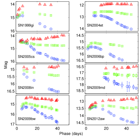
Figure 1.— The $BVI$ light curves of sample SNe. The colors blue, green and red indicate $B$, $V$ and $I$ bands respectively. The phases are in reference to the corresponding time of explosion $t_{\rm ref}$ adopted in table 1.

Table 2Photospheric velocities ($v_{\rm ph}$) of supernovae at different phases.

SN 1999gi			SN 2004et			SN 2005cs			SN 2006bp
Phase	$v_{\rm phs}$	$v_{\rm pha}$	Phase	$v_{\rm phs}$	$v_{\rm pha}$	Phase	$v_{\rm phs}$	$v_{\rm pha}$	Phase	$v_{\rm phs}$	$v_{\rm pha}$
4.7*	13.20 $\pm$ 0.30	12.79	11.1*	8.90 $\pm$ 0.40	8.59	3.4*	6.30 $\pm$ 0.30	6.48	3.35 *	13.70 $\pm$ 0.30	12.99
6.8*	10.30 $\pm$ 0.40	11.09	12.3*	9.10 $\pm$ 0.40	9.54	4.4*	6.10 $\pm$ 0.20	6.04	6.30 *	12.10 $\pm$ 0.20	11.33
7.8*	10.00 $\pm$ 0.40	11.07	13.0*	9.40 $\pm$ 0.40	8.79	5.4*	5.70 $\pm$ 0.25	5.59	8.10 *	11.50 $\pm$ 0.15	11.21
30.7	4.85 $\pm$ 0.07	5.18	14.4*	8.40 $\pm$ 0.40	9.04	8.4*	5.30 $\pm$ 0.30	5.16	10.10*	10.55 $\pm$ 0.20	10.41
35.7	4.20 $\pm$ 0.10	4.67	15.0*	8.80 $\pm$ 0.20	8.31	8.8	5.30 $\pm$ 0.30	4.71	12.13	9.20 $\pm$ 0.40	10.01
38.7	4.05 $\pm$ 0.10	4.47	16.0*	8.00 $\pm$ 0.30	7.79	14.4	4.00 $\pm$ 0.30	3.76	16.10	9.00 $\pm$ 0.50	8.98
89.6	1.60 $\pm$ 0.20	2.78	24.6	7.30 $\pm$ 0.40	6.41	14.4	4.10 $\pm$ 0.20	3.83	21.28	8.10 $\pm$ 0.10	7.69
			30.6	6.20 $\pm$ 0.20	5.69	17.4	3.60 $\pm$ 0.20	3.31	25.26	6.75 $\pm$ 0.30	6.33
			35.5	5.30 $\pm$ 0.30	4.98	18.4	3.60 $\pm$ 0.20	3.52	33.22	6.05 $\pm$ 0.20	5.63
			38.6	5.10 $\pm$ 0.15	4.98	22.5	3.20 $\pm$ 0.50	2.89	42.22	5.05 $\pm$ 0.10	4.79
			40.7	4.90 $\pm$ 0.25	4.86	34.4	2.40 $\pm$ 0.10	2.26	57.20	4.23 $\pm$ 0.05	4.78
			50.5	4.20 $\pm$ 0.25	4.28	36.4	2.25 $\pm$ 0.05	1.80
			55.6	4.00 $\pm$ 0.25	3.85	44.4	1.95 $\pm$ 0.10	1.43
			63.5	3.80 $\pm$ 0.10	3.66	61.4	1.40 $\pm$ 0.07	1.02
						62.4	1.35 $\pm$ 0.13	0.98
SN 2008in			SN 2009bw			SN 2009md			SN 2012aw
Phase	$v_{\rm phs}$	$v_{\rm pha}$	Phase	$v_{\rm phs}$	$v_{\rm pha}$	Phase	$v_{\rm phs}$	$v_{\rm pha}$	Phase	$v_{\rm phs}$	$v_{\rm pha}$
7*	6.10 $\pm$ 0.10	5.72	4.0*	8.90 $\pm$ 0.35	8.90	12	5.50 $\pm$ 0.40	6.22	7*	11.20 $\pm$ 0.30	10.31
14	4.54 $\pm$ 0.15	4.36	17.8	6.70 $\pm$ 0.40	6.84	15	5.30 $\pm$ 0.35	4.76	8*	10.70 $\pm$ 0.30	9.55
54	2.80 $\pm$ 0.07	2.66	19.8	6.15 $\pm$ 0.30	5.66	27	3.05 $\pm$ 0.10	2.92	12*	9.00 $\pm$ 0.35	8.39
60	2.66 $\pm$ 0.06	2.66	33.8	4.85 $\pm$ 0.20	4.68	48	2.05 $\pm$ 0.07	2.22	15*	8.65 $\pm$ 0.30	8.14
			37.0	4.25 $\pm$ 0.25	4.37	100	0.85 $\pm$ 0.10	1.43	16	8.60 $\pm$ 0.25	8.29
			38.0	4.25 $\pm$ 0.15	4.56				20	7.70 $\pm$ 0.20	7.46
			39.0	4.20 $\pm$ 0.10	4.25				26	6.55 $\pm$ 0.20	6.25
			52.0	3.50 $\pm$ 0.20	3.60				31	5.60 $\pm$ 0.10	5.51
			64.0	3.15 $\pm$ 0.10	3.16				45	4.50 $\pm$ 0.06	4.47
			67.0	3.05 $\pm$ 0.10	3.08				55	4.15 $\pm$ 0.08	4.02
									61	3.50 $\pm$ 0.05	3.68
									66	3.50 $\pm$ 0.10	3.61

Notes : Velocity derived using synow is denotated as $v_{\rm phs}$ whereas that by locating the absorption trough as $v_{\rm pha}$. The phases are expressed in days with reference to the $t_{\rm ref}$ adopted in Table 1, while velocities are given in units of $10^{3}\mbox{$\rm{\,km\,s^{-1}}$}$. Velocities at phases marked with astrisks are estimated using He i  lines.

3. data

The sample of type IIP SNe consists of two subluminous SNe 2005cs and 2009md; two normal-luminosity SNe 1999gi and 2012aw; three bright SNe 2004et, 2006bp and 2009bw and a intermediate luminosity SN 2008in having peculiar characteristics. The basic properties of SNe and their host galaxies are given in Table 1. The time of explosion $t_{\rm ref}$ is determined from observational non-detection in optical bands and it is constrained with an accuracy of a day for SNe 2005cs, 2004et and 2012aw, while for the remaining SNe, it is usually constrained by matching the spectra with known template of IIP SNe and the accuracy lies between 2 to 8 days. The total interstellar reddening $E(B-V)_{\rm tot}$ given in Table 1 includes combined reddening due to the Milky way and the host galaxy. For most of these SNe, the value of reddening is constrained quite accurately. Moreover, in this work, values of extinction in different filters (required as input in Eq. 7 and derived using adopted reddening) is estimated assuming the line-of-sight ratio of total-to-selective extinction Rv = 3.1, though a different reddening law towards the sightline of highly embedded SNe cannot be ruled out. We study the implication of variation in reddening on the distance determinations in §4.

The criterion for selecting the present sample has been the availability of photometric and spectroscopic data on at least three phases by 50 days after explosion We restricted the use of data for epm analysis up to the phase 50d, as the value of $\xi$ depends on the color temperature and it varies sharply below 5 kK, i.e. about 50d post explosion for IIP SNe. The $BVI$ photometric data are collected from the literature and Fig. 1 shows the photometric data used in this paper. Barring SN 2009md, we have a dense coverage of early-time ($<50$ day) data for all the events. A typical photometric accuracy for events brighter than 15 mag is 0.02 mag while for fainter events it is poorer.

Table 3EPM derived results for the events.

		D05				H01
		$BV$	$BVI$	$VI$	Mean	$BV$	$BVI$	$VI$	Mean
SN 1999gi	$D$	11.92$\pm$1.08	11.34$\pm$0.34	11.60$\pm$0.86	11.62$\pm$0.29	8.64$\pm$0.80	8.71$\pm$0.31	9.27$\pm$0.73	8.87$\pm$0.34
	$t_{\rm 0}$	1.71$\pm$0.99	2.22$\pm$0.47	1.37$\pm$0.83	1.76$\pm$0.43	2.87$\pm$0.69	2.78$\pm$0.45	1.58$\pm$0.89	2.41$\pm$0.72
SN 2004et	$D$	5.28$\pm$0.23	4.48$\pm$0.13	6.47$\pm$0.26	5.41$\pm$1.00	3.56$\pm$0.17	3.29$\pm$0.10	5.22$\pm$0.22	4.02$\pm$1.04
	$t_{\rm 0}$	0.28$\pm$0.86	4.64$\pm$0.53	0.95$\pm$0.94	1.96$\pm$2.35	2.39$\pm$0.75	5.88$\pm$0.56	1.72$\pm$0.93	3.33$\pm$2.23
SN 2005cs	$D$	7.62$\pm$0.26	7.70$\pm$0.25	8.61$\pm$0.33	7.97$\pm$0.55	5.86$\pm$0.24	5.98$\pm$0.20	6.76$\pm$0.27	6.20$\pm$0.49
	$t_{\rm 0}$	-0.49$\pm$0.68	-0.35$\pm$0.54	-1.77$\pm$0.73	-0.87$\pm$0.78	0.14$\pm$0.73	0.18$\pm$0.51	-1.24$\pm$0.73	-0.31$\pm$0.81
SN 2006bp	$D$	18.82$\pm$1.04	—	—	18.82$\pm$1.04	12.47$\pm$0.57	—	—	12.47$\pm$0.57
	$t_{\rm 0}$	-3.23$\pm$0.77	—	—	-3.23$\pm$0.77	-0.95$\pm$0.50	—	—	-0.95$\pm$0.50
SN 2008in	$D$	13.11$\pm$0.68	14.56$\pm$0.76	15.86$\pm$0.83	14.51$\pm$1.38	12.71$\pm$0.84	11.62$\pm$0.64	12.58$\pm$0.64	12.31$\pm$0.59
	$t_{\rm 0}$	-5.56$\pm$1.34	-6.51$\pm$1.13	-2.84$\pm$1.11	-4.97$\pm$1.91	-11.45$\pm$2.04	-7.01$\pm$1.19	-2.14$\pm$0.96	-6.87$\pm$4.66
SN 2009bw	$D$	15.70$\pm$1.67	16.15$\pm$1.07	22.26$\pm$1.57∗	15.93$\pm$0.32	12.53$\pm$1.39	12.68$\pm$0.98	17.11$\pm$1.36∗	12.61$\pm$0.11
	$t_{\rm 0}$	-0.49$\pm$4.90	-2.27$\pm$1.87	-12.28$\pm$5.69∗	-1.38$\pm$1.26	-2.55$\pm$8.10	-2.46$\pm$2.12	-10.35$\pm$4.25∗	-2.51$\pm$0.06
SN 2009md	$D$	21.06$\pm$4.21	24.09$\pm$3.79	24.72$\pm$3.62	23.29$\pm$1.96	18.74$\pm$3.44	20.29$\pm$3.24	19.29$\pm$2.43	19.44$\pm$0.78
	$t_{\rm 0}$	6.29$\pm$0.46	2.42$\pm$4.78	3.73$\pm$4.00	4.15$\pm$1.97	2.23$\pm$0.46	0.16$\pm$5.18	4.55$\pm$3.16	2.31$\pm$2.19
SN 2012aw	$D$	11.06$\pm$0.44	10.51$\pm$0.21	12.24$\pm$0.49	11.27$\pm$0.88	8.22$\pm$0.35	8.06$\pm$0.16	9.72$\pm$0.43	8.67$\pm$0.92
	$t_{\rm 0}$	-2.55$\pm$0.71	-1.53$\pm$0.32	-2.99$\pm$0.71	-2.36$\pm$0.75	-1.74$\pm$0.61	-0.86$\pm$0.35	-2.44$\pm$0.82	-1.68$\pm$0.79
EPM with fixed explosion epoch
SN 2004et	$D$	5.36$\pm$0.13	5.50$\pm$0.05	6.73$\pm$0.10	5.86$\pm$0.76	4.07$\pm$0.09	4.32$\pm$0.04	5.60$\pm$0.07	4.66$\pm$0.82
SN 2005cs	$D$	7.34$\pm$0.19	7.52$\pm$0.18	7.62$\pm$0.19	7.49$\pm$0.14	5.93$\pm$0.16	6.05$\pm$0.13	6.19$\pm$0.15	6.06$\pm$0.13
SN 2012aw	$D$	9.46$\pm$0.27	9.74$\pm$0.12	10.27$\pm$0.27	9.83$\pm$0.41	7.30$\pm$0.20	7.70$\pm$0.09	8.41$\pm$0.22	7.80$\pm$0.56

Notes: $D$ denotes the distance in Mpc. $t_{0}$ denotes the time of explosion in days, derived in this study and measured with reference to the adopted time of explosion ($t_{\rm ref}$) in Table 1. Negative values of $t_{0}$ indicate dates prior to the adopted value. The values marked with asterisks are considered deviant and these are not considered in computing the mean value.

We obtained the wavelength- and flux-calibrated spectra either from SUSPECT database or from corresponding authors of papers (see Table 1). A typical spectral resolution in the visible range of spectra lies between 5 to 10Å ($\sim$ 300 to 600 $\rm{\,km\,s^{-1}}$at 5500 Å). For SN 2004et, we have also included 6 epoch spectra between +11d to +16d from Takáts & Vinkó (2012). The spectra were corrected for respective recession velocity of their host galaxy before estimating the photospheric velocity. Table 2 provides value of photospheric velocities derived using both the methods described in §2.1, i.e. $v_{\rm pha}$ and $v_{\rm phs}$. A detailed description of the synow modelling of spectra and determination of $v_{\rm phs}$ and its error followed in this work is given elsewhere (Bose et al., 2013). We briefly describe the method below. As we are only interested in obtaining photospheric velocity we fit the observed and synthetic spectra locally around Fe ii  lines (4923.93, 5018.44 and 5169.03 Å) within 4700 - 5300Å, and in early phases where Fe ii  lines are not available we fit around He i  5876Å line within 5500-6200 Å only; since employing the whole wavelength range may introduce over or under-estimation of photospheric velocities as different lines form at different layers. After attaining optimal fit of observed spectra locally, we only vary model parameter $v_{\rm ph}$ to get eye estimate of maximum possible deviation from optimal value and this is attributed as the uncertainty in $v_{\rm ph}$ for that spectrum. We note that as P-Cygni profiles are quite sensitive to $v_{\rm ph}$ and hence the best fits are easily attainable through eye inspection. The typical uncertainty in velocities estimated by deviation seen visually from best-fit absorption troughs varies between 50 to 500 $\rm{\,km\,s^{-1}}$with a typical value of $\sim$ 150 $\rm{\,km\,s^{-1}}$. This is consistent with the values obtained using automated computational techniques viz. $\chi^{2}$-minimization and cross-correlation methods employing entire spectra (Takáts & Vinkó, 2012). A comparison of $v_{\rm pha}$ and $v_{\rm phs}$ is also made and deviations as large as 1000 $\rm{\,km\,s^{-1}}$  is seen in early spectra for a a few SNe, while random deviations are apparent at later epochs to the level of quoted uncertainty. We study implication of using these velocities on the distance determinations in §4.

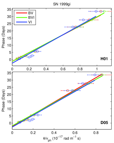
Figure 2.— epm  fitting for SN 1999gi using two sets of dilution factors H01 (top) and D05 (bottom) in combination to three filter subsets BV, BVI and VI. The phases are in reference to the corresponding $t_{\rm ref}$ adopted in table 1.

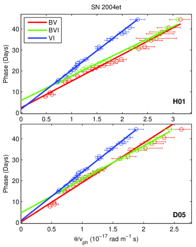
Figure 3.— Same as Fig. 2, but for SN 2004et.

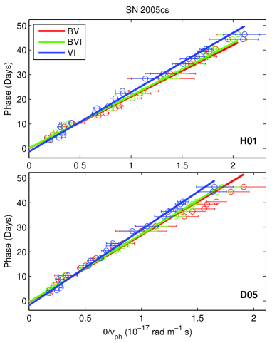
Figure 4.— Same as Fig. 2, but for SN 2005cs.

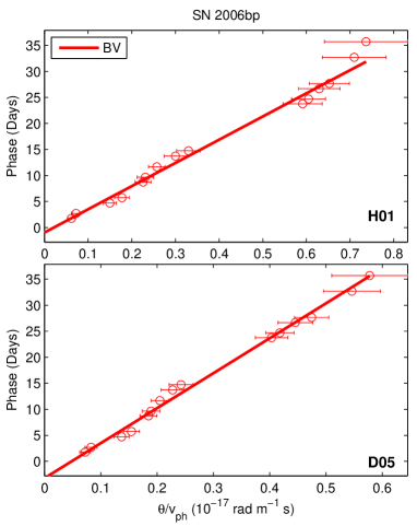
Figure 5.— Same as Fig. 2, but for SN 2006bp using only BV filter subset.

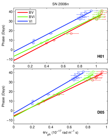
Figure 6.— Same as Fig. 2, but for SN 2008in.

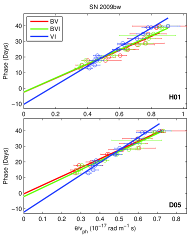
Figure 7.— Same as Fig. 2, but for SN 2009bw.

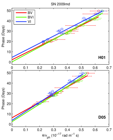
Figure 8.— Same as Fig. 2, but for SN 2009md. Error bars are reduced by factor of five.

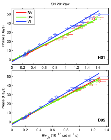
Figure 9.— Same as Fig. 2, but for SN 2012aw.

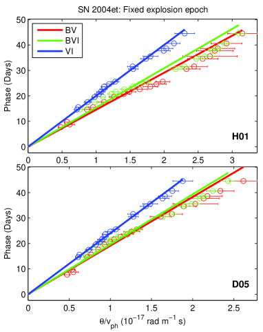
Figure 10.— Same as Fig. 2, but for SN 2004et with fixed explosion epoch at JD 2453270.5.

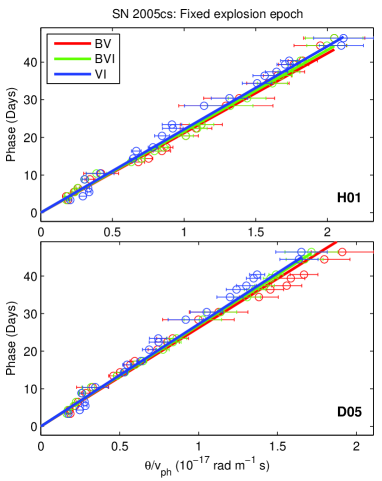
Figure 11.— Same as Fig. 2, but for SN 2005cs with fixed explosion epoch at JD 2453549.0.

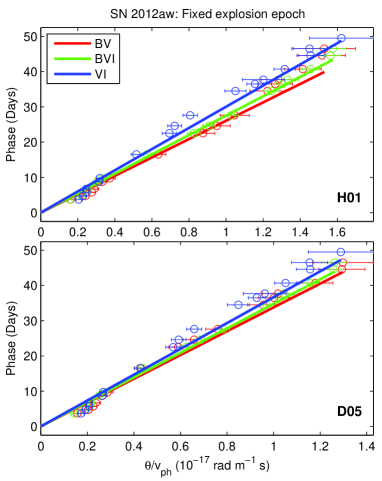
Figure 12.— Same as Fig. 2, but for SN 2012aw with fixed explosion epoch at JD 2456002.6.

4. EPM analysis

At each $t$ for which photometric data is available, we derive the value of $\theta$ for three sets of filter combinations and for two sets of $\xi$ prescriptions. Wherever spectroscopic data do not coincide with the epoch of photometric data point, the value of $v_{\rm ph}$ at $t$ is derived by polynomial interpolation of third or fourth order. It is noted here that in comparison to photometry, spectroscopy of SNe is more demanding in terms of telescope time and as a result, many of our sample have large spectroscopic data gap. In this work, we have therefore, opted to use the interpolated spectroscopic data for the corresponding epoch of photometric data presented in Fig. 1. We performed $\chi^{2}$-minimization for $\theta/v_{\rm ph}$ versus time to derive $D$ and $t_{0}$ (see Eq 1). Here, we use synow-derived value of $v_{\rm ph}$ (i.e. $v_{\rm phs}$, see Table 2). Fig. 2 to 9 show plots for SNe 1999gi, 2004et, 2005cs, 2006bp, 2008in, 2009bw, 2009md, and 2012aw respectively whereas Fig. 10 to 12 show plots to estimate $D$ with fixed $t_{0}$ ($=t_{\rm ref}$, see Table 1) for SNe 2004et, 2005cs and 2012aw.

The results are listed in Table 3. The errors quoted for distance and explosion epoch are mainly contributed by errors in $\theta$ and $v_{\rm ph}$; we discuss errors briefly. Error in quantities $\theta\xi$ and $T$ (see Eq. 7) for a fixed value of $E(B-V)$ are estimated using Monte Carlo technique in which a sample of one thousand data points are drawn from normal distribution of uncertainty in the observed photometric fluxes. Considering that $\xi$ is one dimensional function of temperature only, the error in $\xi$ is numerically estimated using error in $T$. So, the error in $\theta$ is computed by combining errors of $\xi$ and $\theta\xi$ in quadrature. We note that, intrinsically, the factor $\xi$ is a major source of systematic error and it may lead to over or under estimation of epm-derived distance.

The source of error in $v_{ph}$ is random in nature and the relative error in it varies between 2 to 5% whereas in $\theta$ it varies between 5 to 10%. While interpolating velocities at desired photometric epochs, the errors are estimated by Monte Carlo method with a sample size of 1000. For the final epm fit, the error in $\theta/v_{ph}$ is propagated from $\theta$ and $v_{ph}$ and the weighted least-squared fitting is performed to estimate distance and explosion epoch. The error in finally derived distance for each filter subset is estimated by Monte Carlo technique with a sample size of 1000.

It can be seen from Table 3 that for each prescription, we derive three sets of $D$ and $t_{0}$ corresponding to each of the three filter sets. Barring SN 2009bw, the values of $D$ and $t_{0}$ for each of the filter sets are consistent within uncertainties. We, therefore, combine individual distances and explosion epochs derived for each filter set, to compute mean values of $D$ and $t_{0}$ for D05 and H01 $\xi$ prescriptions. The quoted uncertainty in the mean values is the standard deviation of the values obtained for the three filter sets and it can be seen that statistical errors in mean value are consistent with the errors derived in individual filter-sets, barring the case of SN 2009bw which has deviant values for $VI$ set. It can be noted that the relative precision with which epm  distances are derived for either of the atmosphere models (D05 or H01) lies between 2 to 13% having a median value of 6%.

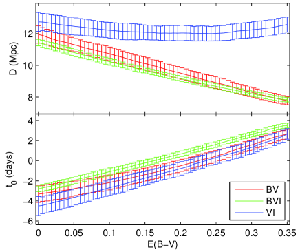
Figure 13.— Variation of epm distances and explosion epoch for each filter sub-set {BV}, {BVI} and {VI} with the variation of E(B-V) for the SN 2012aw using D05 prescription.

Another source of error in $D$ and $t_{0}$ is the value of $E(B-V)$. Though, we have taken its value from literature, and adopted value derived using most reliable method, but its precise determination is extremely difficult and it can introduce systematic error in determination of epm distance. We have studied the effect of $E(B-V)$ for SN 2012aw by varying its value for each filter subset. Figure 13 shows the variation of epm distance and explosion epoch with $E(B-V)$. The variation of distance differs significantly among each filter subset, however the overall variation in distance is not very significant. In order to further study the effect of $E(B-V)$  variation on epm  results for each SNe, we derive mean distances and explosion epochs with the upper and lower limit of $E(B-V)$ and tabulate them in Table 4. We took this approach to estimate deviations of epm results from corresponding $E(B-V)$ errors because of it’s systematic dependence on analysis and we found that it would have been inappropriate to propagate $E(B-V)$ errors all throughout the analysis. It is noted here that epm results have non-linearly dependence on $E(B-V)$ and thus the resulting tabulated errors are asymmetric. The relative variation in $D$ is found to lie between 0 to 9% with median value of 5%.

Table 4Dependence of epm  derived parameters on the errors of $E(B-V)$.

SN event	$E(B-V)$	$D$	$t_{0}$
	(mag)	(Mpc)	(day)
SN 1999gi	$0.21\pm 0.09$	$11.62^{-0.78\pm 0.50}_{+0.93\pm 0.51}$	$~{}~{}1.76^{+0.95\pm 0.49}_{-0.87\pm 0.46}$
SN 2004et	$0.41\pm 0.04$	$~{}5.86^{+0.09\pm 0.96}_{-0.05\pm 0.58}$	$-$
SN 2005cs	$0.05\pm 0.02$	$~{}7.97^{-0.20\pm 0.62}_{+0.11\pm 0.56}$	$-0.87^{+0.37\pm 0.84}_{-0.22\pm 0.93}$
SN 2006bp	$0.40\pm 0.04$	$18.82^{-1.10\pm 1.12}_{+0.99\pm 1.04}$	$-3.23^{+0.94\pm 0.89}_{-0.72\pm 0.77}$
SN 2008in	$0.10\pm 0.10$	$14.51^{-1.13\pm 1.93}_{+1.34\pm 1.81}$	$-4.97^{+1.68\pm 2.18}_{-1.50\pm 1.41}$
SN 2009bw	$0.31\pm 0.03$	$15.93^{-0.62\pm 0.09}_{+0.79\pm 0.50}$	$-1.38^{+0.69\pm 0.57}_{-0.92\pm 1.71}$
SN 2009md	$0.10\pm 0.05$	$23.29^{-0.92\pm 1.88}_{+1.10\pm 2.04}$	$~{}~{}4.15^{+0.56\pm 1.58}_{-0.62\pm 2.27}$
SN 2012aw	$0.07\pm 0.01$	$~{}9.83^{-0.02\pm 0.43}_{+0.00\pm 0.30}$	$-$

The superscript and subscript values in $t_{0}$ and $D$ signify the values derived using upper and lower value of $E(B-V)$ respectively. Further uncertainties quoted in these values are the standard deviation of values obtained from three band sets for each limit of $E(B-V)$.

The references for the values and corresponding errors of $E(B-V)$  are given in Table 1. The errors for SN 2004et and SN 2006bp were unavailable in literature, thus for sake of reasonable approximation, we have attributed 10% error in $E(B-V)$ for these SNe.

Table 5 compares mean value of distances to host galaxies which are taken from ned  and are derived using redshift independent methods, such as Cepheids, Tully-Fisher, Standard Candle Method, Surface Brightness Fluctuation. with that derived using epm . The comparison clearly illustrates that the distance derived using D05 prescription is in better agreement with the ned  ones, whereas the ones using H01 prescription are systematically lower in each of the cases. Similar systematic differences in the two atmosphere models (D05,H01) have also been reported in the EPM implementation to 12 type IIP SNe by Jones et al. (2009).

For D05 models, a comparison of distances derived using $v_{\rm phs}$ and $v_{\rm pha}$, see Table 6, indicate that barring a few cases, there is notable difference in both of the value of distances. For SN 2005cs and 2009md the difference is as high as 18 and 15% respectively, for SN 1999gi, 2004et and 2009bw the values differ by 6 - 9%. However, for SN 2006bp, 2008in and 2012aw the difference is quite negligible and lies in 0 - 3% which is within the internal precision of both values.

EPM analysis of the individual cases are discussed in §5.

Table 5 Comparison of epm  distances to host galaxies with that derived using other methods.

Host	Supernova	$D_{\textsc{epm}}$	$D_{\textsc{ned}}$
Galaxy	Event	(Mpc)	(Mpc)
NGC 3184	SN 1999gi	11.62$\pm$0.29	11.95$\pm$2.71
NGC 6946	SN 2004et	5.86$\pm$0.76	5.96$\pm$1.97
NGC 5194	SN 2005cs	7.97$\pm$0.55	7.91$\pm$0.87
NGC 3953	SN 2006bp	18.82$\pm$1.04	18.45$\pm$1.60
NGC 4303	SN 2008in	14.51$\pm$1.38	16.46$\pm$10.8
UGC 2890	SN 2009bw	15.93$\pm$0.32	—
NGC 3389	SN 2009md	23.29$\pm$1.96	21.29$\pm$2.21
NGC 3351	SN 2012aw	9.83$\pm$0.41	10.11$\pm$0.98

Table 6Comparison of EPM distances derived using synow modeled velocities and from velocities determined by locating the absorption trough.

SN event	$D_{\rm phs}$	$D_{\rm pha}$
	(Mpc)	(Mpc)
SN 1999gi	11.62$\pm$0.29	12.72$\pm$0.47
SN 2004et	5.41$\pm$1.00	4.96$\pm$0.88
SN 2005cs	7.97$\pm$0.55	6.56$\pm$0.42
SN 2006bp	18.82$\pm$1.04	18.13$\pm$1.18
SN 2008in	14.51$\pm$1.38	14.52$\pm$1.39
SN 2009bw	15.93$\pm$0.32	16.92$\pm$0.62
SN 2009md	23.29$\pm$1.96	26.84$\pm$3.78
SN 2012aw	11.27$\pm$0.88	11.27$\pm$0.92

$D_{\rm phs}$ denote epm distances derived using synow model velocities, i.e. $v_{\rm phs}$, whereas, $D_{\rm pha}$ denote the ones derived by locating the absporption minima of Fe ii  lines, i.e. $v_{\rm pha}$. For consistency, the D05 presciption and unconstrained explosion epoch have been used for all the cases.

5. discussions

In the following, we shall discuss results for each of the event and also any anomaly if found in the result.

SN 1999gi : The photometric and spectroscopic data are taken from Leonard et al. (2002b) and the epm-fitting is shown in Fig. 2. For H01 $\xi$ prescription, we derived a distance of $8.87\pm 0.34$ Mpc whereas, Leonard et al. (2002b) and Jones et al. (2009) derived a value of $11.1\pm 2.0$ Mpc and $11.7\pm 0.8$ Mpc respectively. We attribute a lower value of distance in our case to the method adopted in this work i.e. velocity estimates using synow which is significantly different in some epochs and the filter-response deconvolution in SED fitting; and also to less number of data points available for SN 1999gi. Removing first photometric point, our EPM implementation yields a value of $\sim$ 10 Mpc.

For D05 prescription, we derived a value of $11.62\pm 0.29$ Mpc while Jones et al. (2009) derived a value of $17.4\pm 2.3$ Mpc. It is noted that later has excluded the first spectroscopic data point and have used the spectroscopic epochs for epm fitting, in contrast to photometric epochs used in the present work, see §4. Our estimate for D05 is in good agreement with the other redshift independent estimate, see Tab 5.

SN 2004et : We used 21 epochs of photometric data taken from Sahu et al. (2006) and Takáts & Vinkó (2012) to derive epm distance. For this event the time of explosion is determined observationally with an accuracy of a day, and hence, epm fitting is attempted and shown with $t_{0}$ as free and fixed parameters respectively in Fig. 3 and Fig. 10. For D05 prescription, we derive a epm distance of $5.41\pm 1.00$ Mpc and $5.86\pm 0.76$ Mpc respectively; which are consistent with each other as well as with the host galaxy distances derived using other methods. For the former $t_{0}$ is estimated as $1.96\pm 2.35$ days; which is also consistent with the time of explosion adopted from literature ($t_{\rm ref}$). Takáts & Vinkó (2012) derived an epm distance of $4.8\pm 0.6$ using D05 prescriptions and synow velocities.

However, it is noted that the $VI$ fit is quite inconsistent in comparison to the $BV$ and $BVI$ sets. In order to understand this discrepancy, we looked into the possibility of lower value of $E(B-V)$. Sahu et al. (2006) stated that they found equivalent width of 1.7Å for Na I D from low resolution spectra which corresponds to total $E(B-V)$$=0.43$ mag, employing empirical relation of Barbon et al. (1990). On adopting a similar empirical relation by Turatto et al. (2003) which we find more convincing, we arrive at a much lower value of $E(B-V)$ which is 0.26 mag. Being backed by this possibility of lower $E(B-V)$, we re-derive epm distances considering only the Galactic reddening value of 0.29 mag (Schlafly & Finkbeiner, 2011) and arrive to epm distances 5.59, 5.65 and 6.14 Mpc for $BV$, $BVI$ and $VI$ band sets respectively which are fairly consistent with each other. Despite of favorable results with lower $E(B-V)$  we can not rule out the higher value of $E(B-V)$$=0.40$ mag which was derived by Zwitter et al. (2004) using high resolution spectra.

SN 2005cs: We have used 14 epochs spectroscopic and 22 epoch of photometric data from Pastorello et al. (2006, 2009). This is another event for which explosion epoch is constrained observationally within a day hence we have done the fitting by keeping $t_{0}$ as free (Fig. 4) as well as fixed (Fig. 11). We obtain a distance of $7.97\pm 0.55$ Mpc and $7.49\pm 0.14$ Mpc respectively. In case of free $t_{0}$, we arrived at an explosion epoch of $-0.87$ days which is well within uncertainty and consistent with that known observationally. Hence, in this case it is absolutely unnecessary to fix the explosion epoch.

epm has been applied to this SN (Takáts & Vinkó, 2006) and a distance of $7.1\pm 1.2$ Mpc has been determined. However for this a $E(B-V)$=0.11 has been used, the value of reddening was updated to 0.05 by Pastorello et al. (2009) which we adopt in our work, this accounts for the higher value of $D$ estimated in this work. Vinkó et al. (2012) has presented an improved distance estimate of $8.4\pm 0.7$ Mpc for the host galaxy M51 by applying epm on both 2005cs and 2011dh. Another epm estimate for the SN has been presented by Dessart et al. (2008) in which they derived distance of $8.9\pm 0.5$ Mpc. Both of these epm estimates are in good agreement with our results.

SN 2006bp: Photometric data presented by Quimby et al. (2007) is available for $UBVri$ filter, but due to lack of $\xi$ prescriptions for SDSS filter, viz., {BVi} or {Vi}, $ri$ data may not be directly used. We have therefore, carried out epm analysis using {BV} subset only and the results are shown in Fig. 5. For D05 $\xi$ prescription, we derived a distance of $18.82\pm 1.04$ Mpc. Dessart et al. (2008) has also applied epm on the SN in which they estimated the distance using re-computed set of dilution factors and obtained a distance $17.5\pm 0.8$ Mpc which is consistent with our estimate within the limit of errors.

SN 2008in: We used photometric data at 21 epochs from Roy et al. (2011) to estimate epm distance. The spectroscopic coverage of the event is not very good specially within +50 day and hence we had to largely rely upon interpolation (see Table 2). It is noteworthy to mention that we found the velocity of profile of the event is quite less varying and overall velocities are much less as compared to other normal type events. This is also supported by the fact that it is classified as spectroscopically sub-luminous (Roy et al., 2011). The epm fitting is shown in Fig. 6 and we derive a distance of $14.51\pm 1.38$ Mpc and $t_{0}$=$-4.97\pm 1.91$ days for D05 prescription. Utrobin & Chugai (2013) has estimated the explosion epoch for this event using hydrodynamical modelling and estimated an explosion epoch nearly 4 days prior to our adopted reference epoch, thus this shows a very good agreement with EPM estimated $t_{0}$.

SN 2009bw: Fig. 7 shows the epm fitting for this event. It is noted that even though we were having photometric data starting from +5 day (see Fig. 1), but due to single spectra at +4d and unavailability of any other spectra before +18d, we could only include data points within +10 to +50 days for the epm fit. This was necessary to do as in early phase the velocity profile is quite steeper as compared to later phases and thus in such phases velocity interpolation might go wrong due to less number of spectroscopic data.

Using both dilution factor prescription, we find that the distances derived using band sets {BV} and {BVI} are very much consistent with each other, whereas the distance derived using {VI} subset is significantly higher and the explosion epoch is also very much off (see Table 3). Thus making the epm fit of {VI} quite inconsistent with the rest of two band-sets and also the explosion epoch is not consistent with SN age estimated from spectra and light-curve evolution. This particular inconsistency can be justified by the fact that {VI} band-set are at the cooler ends of SED as compared to {BV} and {BVI} band-sets. As in early phase SED is hotter and estimation of SED parameters viz., $\theta$ and temperature, using {VI} band-set will be more prone to errors if the photometric magnitude uncertainty is significant as we have in literature data of SN 2009bw.

Using D05 prescription, we derive a distance of $15.93\pm 0.32$ Mpc. Tully et al. (2009) derive a distance of 11.1 Mpc to the host galaxy using Tully-Fisher method. No other redshift-independent distance estimate is available for this galaxy. We, however, note that Inserra et al. (2012) adopted a distance of 20.2 Mpc based on the redshift of the galaxy.

SN 2009md: Figure 8 shows the epm fit for this event. Extremely large errors in $\theta/v_{ph}$ quantity can be noted and it is attributed entirely due to large photometric errors, as errors in photometric magnitudes have amplified exponentially in fluxes and propagated all throughout to $\theta/v_{ph}$ quantities. Using D05 prescription we obtained a distance of $23.29\pm 1.96$ Mpc and the time of explosion of $4.15\pm 1.97$ days. Fraser et al. (2011) has applied scm to this event and derived a distance of 18.9 Mpc using optical data and of 21.2 Mpc using near infrared data. For this case, the epm result is consistent with that derived using scm.

SN 2012aw: This is a well studied nearby event. The explosion epoch is known fairly accurate with an error of $\pm 0.79$ days, see Bose et al. (2013) and references therein. Figure 12 and Fig. 9 show the epm fit respectively with fixed and free $t_{0}$. For D05 prescription, we derive a distance of $9.83\pm 0.41$ Mpc and $11.27\pm 0.88$ Mpc with explosion $t_{0}=$$-2.36\pm 0.75$. No previous epm  study exist for the galaxy NGC 3351, but recent Cepheids (Freedman et al., 2001) and Tully-Fisher (Russell, 2002) distance estimates are in good agreement with our result.

6. Summary

In this study we present epm distances for eight host galaxies derived using photometric and spectroscopic data of IIP SNe The SNe have mid-plateau absolute V-magnitudes in the range -17 to -15. Detailed epm analysis is done for five of the events, viz., SN 2004et, 2008in, 2009bw, 2009md and 2012aw for the first time. We use two dilution factor models, three filter sub-sets, and two methods for photospheric velocity determination. The value of reddening are known quite accurately and for few of the events the explosion epochs are constrained observationally with an accuracy of a day. We find that epm-derived distances using above two models differs by 30-50%. The epm distances derived using Hamuy’s model (Hamuy et al., 2001) are found to be systematically lower than that of Dessart ones (Dessart & Hillier, 2005). For all the events in our sample, the distances using Dessart model is found to be consistent with that derived using other redshift independent methods, i.e. Tully Fisher, Standard Candle Method, Cepheid, Surface brightness fluctuation. We also note that epm method is applicable only to the early ($<$ 50 d) photometric data of supernovae.

We have also studied the effect of two methods of velocity estimation on the derived distance. It is found that the synow model velocities are significantly different than that estimated by locating absorption trough of P-Cygni. The distances derived from two different velocity determination methods have notable differences as high as 15-18%, however we did not find any systematic trend of this difference. This suggests the difference is the direct effect of the measurement error of absorption minima method when the photospheric lines are blended or weak relative to continuum.

References

- Arcavi et al. (2010) Arcavi, I., et al. 2010, ApJ, 721, 777
- Arnett (1996) Arnett, D. 1996, Supernovae and Nucleosynthesis: An Investigation of the History of Matter from the Big Bang to the Present
- Barbon et al. (1990) Barbon, R., Benetti, S., Rosino, L., Cappellaro, E., & Turatto, M. 1990, A&A, 237, 79
- Baron et al. (2007) Baron, E., Branch, D., & Hauschildt, P. H. 2007, ApJ, 662, 1148
- Baron et al. (2004) Baron, E., Nugent, P. E., Branch, D., & Hauschildt, P. H. 2004, ApJL, 616, L91
- Bessell (1990) Bessell, M. S. 1990, PASP, 102, 1181
- Bose et al. (2013) Bose, S., et al. 2013, MNRAS, 433, 1871
- Branch et al. (2002) Branch, D., et al. 2002, ApJ, 566, 1005
- Burrows (2013) Burrows, A. 2013, Reviews of Modern Physics, 85, 245
- Dessart et al. (2008) Dessart, L., et al. 2008, ApJ, 675, 644
- Dessart & Hillier (2005) Dessart, L., & Hillier, D. J. 2005, A&A, 439, 671
- Dessart & Hillier (2006) Dessart, L., & Hillier, D. J. 2006, A&A, 447, 691
- Eastman et al. (1996) Eastman, R. G., Schmidt, B. P., & Kirshner, R. 1996, ApJ, 466, 911
- Elmhamdi et al. (2003) Elmhamdi, A., et al. 2003, MNRAS, 338, 939
- Filippenko (1997) Filippenko, A. V. 1997, ARA&A, 35, 309
- Fisher et al. (1999) Fisher, A., Branch, D., Hatano, K., & Baron, E. 1999, MNRAS, 304, 67
- Fisher et al. (1997) Fisher, A., Branch, D., Nugent, P., & Baron, E. 1997, ApJL, 481, L89
- Fraser et al. (2011) Fraser, M., et al. 2011, MNRAS, 417, 1417
- Freedman et al. (2001) Freedman, W. L., et al. 2001, ApJ, 553, 47
- Gandhi et al. (2013) Gandhi, P., et al. 2013, ApJ, 767, 166
- Hamuy (2003) Hamuy, M. 2003, ApJ, 582, 905
- Hamuy & Pinto (2002) Hamuy, M., & Pinto, P. A. 2002, ApJL, 566, L63
- Hamuy et al. (2001) Hamuy, M., et al. 2001, ApJ, 558, 615
- Heger et al. (2003) Heger, A., Fryer, C. L., Woosley, S. E., Langer, N., & Hartmann, D. H. 2003, ApJ, 591, 288
- Hopkins & Beacom (2006) Hopkins, A. M., & Beacom, J. F. 2006, ApJ, 651, 142
- Immler et al. (2007) Immler, S., et al. 2007, ApJ, 664, 435
- Inserra et al. (2011) Inserra, C., et al. 2011, MNRAS, 417, 261
- Inserra et al. (2012) Inserra, C., et al. 2012, MNRAS, 422, 1122
- Janka (2012) Janka, H.-T. 2012, Annual Review of Nuclear and Particle Science, 62, 407
- Jones et al. (2009) Jones, M. I., et al. 2009, ApJ, 696, 1176
- José & Iliadis (2011) José, J., & Iliadis, C. 2011, Reports on Progress in Physics, 74, 096901
- Kasen & Woosley (2009) Kasen, D., & Woosley, S. E. 2009, ApJ, 703, 2205
- Kirshner & Kwan (1974) Kirshner, R. P., & Kwan, J. 1974, ApJ, 193, 27
- Leonard et al. (2002a) Leonard, D. C., et al. 2002a, PASP, 114, 35
- Leonard et al. (2002b) Leonard, D. C., et al. 2002b, AJ, 124, 2490
- Leonard et al. (2003) Leonard, D. C., Kanbur, S. M., Ngeow, C. C., & Tanvir, N. R. 2003, ApJ, 594, 247
- Olivares E. et al. (2010) Olivares E., F., et al. 2010, ApJ, 715, 833
- Pastorello et al. (2006) Pastorello, A., et al. 2006, MNRAS, 370, 1752
- Pastorello et al. (2009) Pastorello, A., et al. 2009, MNRAS, 394, 2266
- Poznanski (2013) Poznanski, D. 2013, ArXiv e-prints
- Quimby et al. (2007) Quimby, R. M., Wheeler, J. C., Höflich, P., Akerlof, C. W., Brown, P. J., & Rykoff, E. S. 2007, ApJ, 666, 1093
- Roy et al. (2011) Roy, R., et al. 2011, ApJ, 736, 76
- Russell (2002) Russell, D. G. 2002, ApJ, 565, 681
- Sahu et al. (2006) Sahu, D. K., Anupama, G. C., Srividya, S., & Muneer, S. 2006, MNRAS, 372, 1315
- Schlafly & Finkbeiner (2011) Schlafly, E. F., & Finkbeiner, D. P. 2011, ApJ, 737, 103
- Schmidt et al. (1992) Schmidt, B. P., Kirshner, R. P., & Eastman, R. G. 1992, ApJ, 395, 366
- Schmidt et al. (1994) Schmidt, B. P., Kirshner, R. P., Eastman, R. G., Phillips, M. M., Suntzeff, N. B., Hamuy, M., Maza, J., & Aviles, R. 1994, ApJ, 432, 42
- Smartt (2009) Smartt, S. J. 2009, ARA&A, 47, 63
- Smartt et al. (2009) Smartt, S. J., Eldridge, J. J., Crockett, R. M., & Maund, J. R. 2009, MNRAS, 395, 1409
- Smith et al. (2011) Smith, N., Li, W., Filippenko, A. V., & Chornock, R. 2011, MNRAS, 412, 1522
- Takáts & Vinkó (2006) Takáts, K., & Vinkó, J. 2006, MNRAS, 372, 1735
- Takáts & Vinkó (2012) Takáts, K., & Vinkó, J. 2012, MNRAS, 419, 2783
- Tully et al. (2009) Tully, R. B., Rizzi, L., Shaya, E. J., Courtois, H. M., Makarov, D. I., & Jacobs, B. A. 2009, AJ, 138, 323
- Turatto et al. (2003) Turatto, M., Benetti, S., & Cappellaro, E. 2003, in From Twilight to Highlight: The Physics of Supernovae, ed. W. Hillebrandt & B. Leibundgut, 200
- Utrobin & Chugai (2013) Utrobin, V. P., & Chugai, N. N. 2013, ArXiv e-prints
- Vinkó & Takáts (2007) Vinkó, J., & Takáts, K. 2007, in American Institute of Physics Conference Series, Vol. 937, Supernova 1987A: 20 Years After: Supernovae and Gamma-Ray Bursters, ed. S. Immler, K. Weiler, & R. McCray, 394
- Vinkó et al. (2012) Vinkó, J., et al. 2012, A&A, 540, A93
- Wagoner (1981) Wagoner, R. V. 1981, ApJL, 250, L65
- Woosley & Weaver (1995) Woosley, S. E., & Weaver, T. A. 1995, ApJS, 101, 181
- Zwitter et al. (2004) Zwitter, T., Munari, U., & Moretti, S. 2004, IAU Circ., 8413, 1