A real-time simulation facility for astronomical adaptive optics

Abstract

In this paper we introduce the concept of real-time hardware-in-the-loop simulation for astronomical adaptive optics, and present the case for the requirement for such a facility. This real-time simulation, when linked with an adaptive optics real-time control system, provides an essential tool for the validation, verification and integration of the Extremely Large Telescope real-time control systems prior to commissioning at the telescope. We demonstrate that such a facility is crucial for the success of the future extremely large telescopes.

1 Introduction

All ground-based astronomical telescopes perform science by observing through the Earth’s atmosphere, which has a degrading effect on the images obtained in the optical and near infrared. Adaptive optics (AO) (Babcock, 1953) is a technology employed on most major telescopes which seeks to remove some of the effects of atmospheric turbulence, producing clearer, high resolution science images as a result. It is a crucial technology for the next generation Extremely Large Telescope (ELT) facilities (Spyromilio et al., 2008) which will spend the significant majority of their time producing AO corrected observations.

1.1 The ELT AO system integration problem

The design process of an AO system involves extensive numerical simulation and modelling. At the scale of the systems required for the ELTs, this modelling is an extremely time consuming process using currently available tools. It can often take many hours to cover a single point of the large explorable parameter space, making responsive design decisions difficult.

Once these systems have been designed and the components fabricated, verification and integration with ELT facilities is required, followed by instrument commissioning. Herein lies a significant problem: The ELT AO systems will be dependent on major components that form part of the ELT design, for example the M4 mirror for the European ELT (E-ELT), and an extensive laser guide star (LGS) launch capability, as well as a large number of expensive, technically advanced wavefront sensors (WFSs). Not only are these components expensive, they are often also physically large, and so using them during laboratory AO system integration would result in huge cost and complication. The complexities of ELT-scale AO systems means that the design and build of these systems is likely to take place at multiple sites around the world. Therefore, if multiple copies of components are required (including dummy components, for example a non-deformable mirror of an equivalent size), this will also greatly add to the cost of the instruments. The wide-field, laser assisted AO systems proposed for operation with most ELT instruments also require large numbers of fast, low noise wavefront sensors. These state-of-the-art components are expensive, and likewise it would not be possible to duplicate them across every AO laboratory involved with the design and build of the AO system in question. The real-time control system (RTCS) which provides deformable mirror (DM) commands in response to WFS inputs requires these components to be present so that optical and electrical feedback loops and calibration procedures can be implemented and tested. In addition, this RTCS is integral to the end-user tools required for AO system operation, and therefore is required for the development and testing of these tools. Subsystem integration at the telescope itself is also not a solution due to the high costs of ELT time.

In this paper, we develop a solution for this currently unsolved verification, integration and commissioning problem for ELT AO instruments. We also comment on the additional benefits that this solution will bring to the AO community. In §2 we introduce the concept of a real-time hardware-in-the-loop simulation capability focused on enabling test, verification and integration of ELT AO systems. In §3 we consider case studies where we have used a simulation to real-time control link, and where hardware-in-the-loop simulation is essential. We conclude in §4.

2 Real-time AO simulation

The impracticalities associated with using the large physical components of an ELT AO system for verification and integration lead to the conclusion that simulation of these components is necessary. On the one hand, these components could be replaced with a physical dummy version that simply provides or accepts the equivalent electronic signals. This however only allows interface testing, and does not allow full system testing, for example, of:

1. Algorithms within the RTCS.

2. Calibration procedures for performance optimisation.

3. Closed loop latency, bandwidth and jitter tests.

4. Real-time response of the RTCS.

5. Stress-testing of the system under typical usage patterns.

6. Interaction with telescope facilities.

Therefore, a hardware-in-the-loop simulation model of these components is also required (Fig. 1). Not only must these simulation models interface to the RTCS, they must also interact with any physical components present, and must be able to operate at real-time rates to allow proper testing of the RTCS subsystems. This facility will also be useful for AO systems on existing telescopes, and is therefore not restricted to ELT systems.

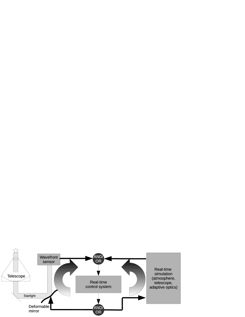
Figure 1: A diagram showing the concept of a real-time simulation capability. The real-time control system is able to use a mixture real and modelled components.

AO simulation, using Monte-Carlo techniques, is routinely used to model the performance of ELT AO systems (Basden et al., 2013; Wang & Ellerbroek, 2012). These models, which include the effect of atmospheric turbulence, sensor noise and physical models for WFS cameras, DMs and science cameras are highly computationally intensive. Efforts have been made to use non-conventional computing hardware (Basden et al., 2005; Gratadour et al., 2013) to increase the speed of AO simulations, thus reducing the time taken to explore a given parameter space. Additionally, recent advances in conventional computing technologies, including graphical processing units (GPUs) and many-core technologies increase the potential for a further reduction in simulation execution times. However, to allow an ELT-scale AO simulation to reach real-time rates would require a substantial computational hardware investment, which may not always be possible or appropriate. We therefore propose a five step plan for development of a real-time hardware-in-the-loop AO simulation capability, outlined in the following sections. Each of these steps should be considered as a solution to a subset of problems in its own right, and it is not necessary to implement all steps for every instrument or at every laboratory, allowing a cost and complexity trade-off to be made.

It is important to note that this real-time hardware-in-the-loop simulation facility is not designed with the goal of high fidelity AO simulation, or for parameter space investigation or new algorithm development. Rather it is aimed at solving the AO system integration issues when faced with complicated telescope interfaces and components not present during laboratory integration, to reduce the risks associated with AO system development.

2.1 Interfacing of simulation with a real-time control system

The first step to be taken towards solving the ELT AO verification, integration and commissioning problem is to interface a full Monte-Carlo simulation code with the AO RTCS. This should be implemented in a way which allows the RTCS to be blind to the fact that it is operating in simulation mode, i.e. all the RTCS algorithms should be as intended for on-sky use. This is essential because it allows algorithms that are not implemented within typically Monte-Carlo simulations, yet which greatly improve on-sky performance, to be fully investigated and tested, such as adaptive windowing techniques and brightest pixel selection (Basden et al., 2012).

At this step, the simulated components will not be operated at real-time rates, allowing conventional PC hardware to be used for the simulation, without requiring massive parallelisation techniques. This will allow the AO loop to be engaged within the RTCS, and performance metrics obtained. Costs will be minimised, and so this step is appropriate for wide distribution to laboratories involved with AO system development for who real-time operation is not essential. This is demonstrated in Fig. 2(a). We suggest that this step is particularly appropriate for AO systems on 10 m class telescopes where reasonable simulation frame rates are achievable on modest computational hardware.

Figure 2: A diagram demonstrating some of the stages of hardware-in-the-loop real-time simulation. (a) Step one, a simulation interfaced with a RTCS. (b) Step two, a fast simulation interfaced with a RTCS. (c) Step three, a real-time simulation interfaced with a RTCS. (d) Step four, physical component interchange and modelling (here showing a missing WFS, spot modification of a physically present WFS, and a missing DM).

We have demonstrated this step by interfacing the Durham AO simulation platform (DASP) (Basden et al., 2007) with the Durham AO real-time controller (DARC) (Basden et al., 2010; Basden & Myers, 2012), which has provided an ideal tool for developing and testing on-sky algorithms used in the CANARY instrument (Gendron et al., 2011). In this case, the link between simulation and RTCS was implemented using Ethernet sockets rather than the serial Front Panel Data Port (sFPDP) communication used by the WFS cameras. Thus, to change between real and simulation mode, it is necessary to load and unload the relevant DARC modules within the RTCS. However, due to the design of DARC, such modularity is trivial, and no algorithm changes are required.

In this first step of real-time simulation, it should be noted that there are no physical components. The atmosphere, telescope, WFSs, optics and DMs are all simulated. For a RTCS that can operate entirely within a PC (such as DARC, when using appropriate modules), this step allows the whole RTCS and simulation to be operated on a single PC, providing ultimate flexibility, suitable for duplication by many developers simultaneously.

In addition to providing a test harness for the RTCS with all the hardware components (albeit simulated), this real-time simulation interface has a further advantage over laboratory test-bench demonstration: The ability to explore a far wider atmospheric turbulence parameter space. This includes the simulation of a far greater number of atmospheric phase screens than are available with a typical test bench. We have simulated up to 40 phase screens at ELT-scale using DASP, while a typical laboratory setup will contain up to four screens (Reeves et al., 2012). This provides the ability to model velocity dispersion within layers, and also to model layers with finite thickness, allowing real-time implementations of key algorithms to be tested.

2.1.1 Playback of images and slopes

At this step, we include the ability to replay pre-generated WFS images into the RTCS, and also the possibility of replaying pre-recorded wavefront slope measurements, should the RTCS be able to accept this. This would allow some validation (particularly of some wavefront reconstruction algorithms) to be implemented by comparing RTCS output with the expected output.

2.2 Fast simulation

The next step is for moderate acceleration of the simulation code, using hardware that is readily available and affordable, comprised of typically a small number of GPU accelerated computer servers as shown in Fig. 2(b). Although this adds to the complexity of the simulated system, it has the advantage that the system update rate will be up to a few tens of Hertz for an ELT-scale instrument, allowing users to control the RTCS without unacceptable delays, and to view telemetry data (WFS images, reconstructed phase, etc.) at a rate that is acceptable to the human eye, allowing users to better appreciate how the AO system will operate as a whole, and providing a reasonable responsiveness to user interface controls.

2.3 Real-time simulation

To achieve real-time rates for an AO simulation and RTCS combination at ELT-scale, greater computational resources will be required, consisting of a moderate computing cluster as shown in Fig. 2(c). Here we provide an estimate of the required computing power for a typical ELT instrument reminiscent of the proposed ELT Adaptive optics for GaLaxy Evolution (EAGLE) instrument (Evans et al., 2008), and consider the hardware that would be required to implement a real-time simulation capability. We do not consider here the requirements for the RTCS itself, as this has been covered elsewhere (Basden & Myers, 2012).

A real-time simulation harness for an ELT RTCS is essential to solve the verification, integration and test problem that has been identified for the ELTs. This will provide a facility to allow the full RTCS to be integrated with ELT systems prior to arrival at the telescope.

2.3.1 Simulation components

A real-time simulation facility must model many separate components so that a realistic test harness for the RTCS can be provided. These include as a bare minimum:

1. Wavefront phase distortions caused by layers of atmospheric turbulence (up to 40 layers are required for accurate modelling, Costille & Fusco (2012))

2. The integrated phase distortions along given lines-of-sight

3. Telescope and WFS optics (including LGS spot elongation)

4. WFS noise

5. DMs and associated optical components

6. Science cameras for performance verification

Since the real-time simulation must operate for undetermined periods of time, we assume that a technique for generating infinitely long atmospheric phase screens will be used (Assémat et al., 2006), based on the statistical co-variance of the turbulent phase.

2.3.2 Computational complexity

We now consider the minimum computational requirements that will be required for an ELT-scale real-time simulation of an AO instrument operating at 250 Hz (that of EAGLE). An estimate for the required operations are given in table 1 for a single line-of-sight, turbulent layer or WFS. However, it should be noted that this will vary depending on simulation input parameters, such as number of turbulent atmospheric layers, layer heights, wind velocities, WFS pixel scale and many other factors, so should only be treated as representative. Additionally, we have only considered the basic algorithms required, and it is likely that a true real-time simulation would require extra algorithms to improve fidelity. We also assume that data accesses are for data that is contiguous in memory, or that stepped memory access is available (as with the Intel Sandy Bridge processors). The required operations match those that we currently use in DASP.

Table 1: A table detailing the operations required for real-time simulation. Where available, operations are given as standard BLAS function names. Memory access is given in 4-byte units. $N$ is the number of phase pixels across the telescope pupil ( 1600 for EAGLE), and $M$ is the number of sub-apertures across the telescope pupil ( 80 for EAGLE).

Algorithm	Operations	Complexity	Memory access	EAGLE at 250 Hz
Phase screen generation	Per layer: 2 GEMV, 1 AXPY	$16N^{2}+2N$	$8N^{2}+2N$	10 GFLOPS, 20 GBs-1
Line-of-sight integration	Per layer and direction: 2D-spline interpolation, AXPY	$N^{2}\ln N+N^{2}$	$2N^{2}$	5 GFLOPS, 4 GBs-1
WFS model	Per WFS: 2 AXPY, Cos/Sin, 2D FFT, 2D convolution, AXPY, Noise addition	$13N^{2}+3N^{2}\ln M$	$5N^{2}$	16 GFLOPS, 12 GBs-1
DM model	Per DM and direction: 2D-spline interpolation, AXPY	$N^{2}\ln N+N^{2}$	$2N^{2}$	5 GFLOPS, 4 GBs-1
Science	Per science direction: 3 AXPY, Cos/Sin, 2D FFT, SUM	$10N^{2}+N^{2}\ln N$	$6N^{2}$	11 GFLOPS, 15 GBs-1

Using these computational complexity estimates, we can place an order of magnitude estimate on the simulation computational requirements for ELT AO systems, as shown in table 2. If we assume that the real-time simulation is to be implemented using GPU technology, then estimates can be placed on the size of a system required to implement this real-time simulation. The current generation of GPUs, such as the NVIDIA GTX-780 can reach approximately 4 TFLOPS of single precision floating point performance, and have a theoretical internal memory bandwidth of up to 250 GBs^-1. This internal memory bandwidth is therefore the limiting factor in real-time simulation performance. If we assume that for mixed algorithms, 50% of the theoretical bandwidth peak can be reached (Basden & Myers, 2012), then three of the cases in table 2 are achievable using 18 GPUs. The most demanding case (a 40 layer simulation) would require about 50 GPUs. A suitable system would contain several PCs to host these GPUs, and thus require inter-node communications. This introduces additional complexity to the system, requiring time for the transmission and marshalling of data. We therefore suggest that additional computing power is required to reduce computation time, thus allowing additional time for data communications (which we do not cover here). Some overhead is also necessary to allow for communication with the RTCS. A factor of two would seem reasonable, requiring a 36 GPU system to obtain real-time simulation rates for models with ten atmospheric layers.

The ELT simulation problem is highly suitable for parallelisation, and will benefit from improvements made in future computational hardware. Not only is it possible to parallelise at the component level (WFSs, phase screens, DMs etc.), but it is also possible to split computation of many components across different computational hardware units, with clean partitioning between units requiring little or no inter-unit communication. As an example, WFS sensor simulation can be divided easily on a per-sub-aperture basis, producing sections of WFS images on separate GPUs before marshalling to produce the final image to be sent to a real-time control system. Such marshalling is trivial when GPUs are on the same host, and requires additional network bandwidth when generated on separate hosts. Currently, up to eight GPUs can be used with a single host on commonly available motherboards.

Almost all parts of AO simulation can either be parallelised in this way or can be generated identically in different parts of the simulation hardware where there is potential to increase simulation speed by reducing network bandwidth requirements. For example it may be preferable to generate multiple instances of the same atmospheric phase screen, rather than distributing one instance to all the simulation components that require it.

Scaling of algorithms across multiple GPUs is a well known technique, which in the case of some well suited algorithms, provides performance improvements almost proportional to the number of GPUs used. In typical real-world applications, scaling is slightly worse. Figure 3 shows performance scaling with number of GPUs of the DARC RTCS configured for a $84\times 84$ sub-aperture AO system with 3 DMs (a total of 9700 actuators). Here, the GPUs were used for wavefront reconstruction, and although algorithms used for simulation are different, we take this as representative of real-world algorithms used for AO. In this case, WFS calibration and slope calculation were performed in central processing unit (CPU) which will also have some effect on the system scaling. The scaling that we achieve is similar to that reported for GPU accelerated AO simulation (Gratadour et al., 2013), with performance scaling slightly worse than proportional to the number of GPUs present.

Figure 3: A figure showing scaling of real-time control system performance as a function of number of GPUs used, based on results obtained using the DARC system configured for an ELT case.

The theoretical scaling of computational requirements as a function of AO system size can be obtained from table 1. We have investigated RTCS performance scaling using DARC with reconstruction performed using a single GPU, and other operations performed on the host processor. Results are shown in Fig. 4(a), and although these algorithms are different from those that would be required in simulation, demonstrate scaling with system size. Previous studies of single conjugate AO (SCAO) simulation (Gratadour et al., 2013) have investigated scaling of simulation with AO system order on GPU, and from this information we have computed simulation time (excluding slope estimation and wavefront reconstruction), as shown in Fig. 4(b). This includes most of the algorithms required for hardware-in-the-loop simulation, demonstrating a scaling proportional to square of telescope diameter, in agreement with table 1.

Figure 4: (a) A figure showing scaling of real-time control system performance as a function of telescope size using a single GPU for wavefront reconstruction, assuming 0.5 m sub-apertures. A quadratic fit is shown in grey. (b) Showing scaling of AO simulation as a function of telescope size, using data from (Gratadour et al., 2013).

Random access memory (RAM) in the current generation of GPUs is limited to about 6 GB, while the ELT scale simulations that we use require up to 32 GB RAM. A real-time simulation facility would be spread across many GPUs, and so we do not foresee any memory problems arising, since the simulation can be naturally partitioned and parallelised in such a way that memory consumption is spread out between the GPUs. In the fast (non-real-time) simulation case, fewer GPUs will be used, possibly containing less than 32 GB between them. However, the idea in this case is that the GPUs are then used for offloading parts of the simulation computation, not all of it, and so available memory is likely to be sufficient. Future generations of GPUs and many-core processors are likely to have more memory (for example the Intel Xeon Phi has 16 GB), further alleviating any memory problem.

Table 2: A table estimating real-time simulation computational requirements for different proposed E-ELT instruments.

Instrument	# layers	# WFS	# DMs	Frame rate	Requirements	Ref
EAGLE	10	11	20	250	2.1 TFLOPS, 2.0 TBs-1	(Basden et al., 2013)
EAGLE	40	11	20	250	7.1 TFLOPS, 6.3 TBs-1	(Basden et al., 2013)
MAORY	10	9	3	500	1.7 TFLOPS, 1.6 TBs-1	(Foppiani et al., 2010)
MAORY	40	9	3	500	5.9 TFLOPS, 5.7 TBs-1	(Costille & Fusco, 2012)
ATLAS	10	8	1	800	2.2 TFLOPS, 2.2 TBs-1	(Fusco et al., 2010)
ATLAS	40	8	1	800	7.5 TFLOPS, 7.5 TBs-1	(Costille & Fusco, 2012)

Although our treatment of computational requirements has been preliminary, we have nevertheless been able to show that an ELT-scale real-time simulation capability is achievable using existing computational hardware, though our estimates for hardware required are order-of-magnitude only.

2.3.3 Accuracy and performance trade-offs

In order to achieve real-time rates on available hardware, it may be necessary to reduce accuracy of the simulations. This will have some impact on the AO system performance, depending on what simplifications are made. However, since this real-time simulation facility is focused on ELT system integration rather than high fidelity simulation this is unlikely to cause problems in most situations. When high fidelity simulations are required, the simplifications can be removed, resulting in a fast (but not real-time) AO simulation capability.

An example of an accuracy and performance trade-off that can made is that of telescope pupil sampling for phase-screen generation. Reducing the sampling reduces both the computational requirements for the simulation, and also the accuracy of the simulation. Another example is the number of atmospheric layers modelled. Fewer layers would result in reduced simulation fidelity, though with lower computational cost. How far each trade-off can be taken will depend on the particular circumstances under investigation.

DM modelling fidelity is also a trade-off that can be made to reduce computational complexity. Simplified models for DMs will result in less accurate simulations though enable real-time rates with reduced hardware requirements. Similarly, wavefront sensor models can also be simplified at the expense of accuracy, for example by ignoring vignetting, and by using pre-generated, or simplified random noise generators to model detector readout noise.

Elongation of LGS spots is also another area where simulations can be simplified to reduce computational requirements, including sodium profile sampling and the size of resulting sub-aperture images.

Single precision floating point operation is sufficient for almost all aspects of ELT simulation, and is what we currently use for our AO simulations. The exception is for infinite phase-screen generation which requires double precision accuracy to maintain valid statistics.

2.4 Physical component interchange and modelling

So far we have considered only cases where there are no physical components present, i.e. all such items, including DMs and WFSs are modelled in simulation. However, an additional step can also be taken to allow physically present components to be used with the RTCS, and absent components to be modelled. Examples include systems with a sub-set of WFSs present, or systems with one or more DMs absent, as illustrated in Fig. 2(d).

The combination of physical and modelled components introduces an extra degree of complexity for the modelling, and thus increased computational requirements if real-time rates are to be maintained.

2.4.1 Absent wavefront sensors

Let us first consider the case where not all WFSs are present at the AO system integration laboratory. This situation is particularly likely to arise for wide-field tomographic AO systems which require a large number of high-speed, low noise WFSs, with cost preventing replication of the complete set of WFSs at all integration facilities. It is therefore necessary to use hardware-in-the-loop simulation of the missing WFSs, to enable RTCS integration. If the atmospheric turbulence is deterministic, for example it is created using a system of rotating phase screens or a set of liquid crystal screens, then accurate simulation models can be created. It is possible to determine exactly what wavefront aberrations are being introduced (if necessary by correlating the expected wavefront with reconstructed phase from the physically present WFSs), thus allowing simulation of the corresponding non-present WFSs, which would then deliver WFS images to the RTCS almost identical to images that would have been produced if the physical WFS had been present. The RTCS can then be used to perform standard tomographic reconstruction and DM control, as if all physical WFSs were present.

In the case where the atmospheric turbulence is not deterministic, this technique cannot be used. Depending on the requirements for the system (whether tomographic reconstruction and science verification is required), other techniques may be possible, for example duplicating WFS information (using copies of images from physically present WFSs to model the absent WFSs), or by using the physically present WFSs to perform a tomographic wavefront reconstruction, from which the absent WFSs can be simulated.

For close-loop AO systems, the real-time simulation code can also be informed about the shape of the DMs, thus allowing the simulated WFSs to also respond to DM surface changes.

2.4.2 Absent deformable mirrors

We now consider the case where all WFSs are present, but one or more DM is not, for example the E-ELT M4 mirror, which is physically large and not well suited to laboratory integration. We assume that the missing DMs are before the WFSs in the optical path, i.e. changes to the DM surface are measurable using the WFSs. If this is not the case (e.g. some DMs in an open-loop multi-object AO (MOAO) system) the problem is actually easier to solve, affecting science verification only.

An accurate model of the desired DM surface shape can be obtained using the RTCS outputs, and the amount of detail in these models (for example assuming a perfect DM or including hysteresis, non-linearities and mis-alignments) will depend on circumstances and requirements. It is then possible to model how this optical surface would affect the physical Shack-Hartmann WFS images relative to an input plane wave, allowing individual sub-aperture point spread functions (PSFs) to be computed. A convolution of these PSFs with the real WFS images then yields a good approximation to the WFS images that would have been obtained when a physical DM was present as shown in Fig. 5. The presence of WFS noise reduces the fidelity of this approximation, though in an integration laboratory, WFS signal levels can usually be increased, with statistical noise added back into the real-time simulation images after this correlation. These modified WFS images are then used as input for the RTCS, and we call this process “active spot modification”.

Figure 5: A figure showing the accuracy of the active spot modification technique. The curves show the RMS difference between slopes measured when a DM is not present but simulated, to slopes measured when a DM is present. The solid curve represents Shack-Hartmann images modified using the active spot modification, while the dashed curve represents Shack-Hartmann images through turbulence alone (i.e. without DM simulation, and hence no spot modification).

The key benefit of this technique is that it allows the whole AO RTCS to be tested in the absence of a small number of critical components.

2.4.3 Active spot modification

The “active spot modification” technique allows RTCS testing of extended WFS PSFs in laboratory situations where such PSFs are difficult to generate optically, for example for elongated laser spots (Lardière et al., 2008). The key concept is to take a closed-loop laboratory AO system and modify wavefront sensor images on a per-sub-aperture basis to allow testing of algorithms within the RTCS. This active modification can include the addition of simulated photon shot noise, variations in signal intensity, and detector readout noise. Investigation of AO performance scaling with signal level can be carried out (allowing finer changes in signal than can be achieved using neutral density filters for example), and also allows the effect of rapid signal level changes on RTCS performance to be investigated.

To use this technique with maximum effect, the true (laboratory) illumination level needs to be sufficiently bright to be in the high light level regime (essentially noiseless), which in a laboratory situation, is usually possible using bright sources. Similarly, the WFS detector pixels should be Nyquist sampled for this technique to work well.

Figure 5 was generated using a simulation of the atmosphere and a DM on a $10\times 10$ sub-aperture AO system on a 4.2 m telescope. The modelled WFS was assumed to have 0.1 electrons root-mean-square (RMS) readout noise, and a standard centre of gravity algorithm was used to compute wavefront slope.

A random shape was applied to the surface of the $11\times 11$ actuator DM, the surface shape of which was obtained using cubic spline interpolation. An atmospheric phase screen was generated using a Von Karman spectrum (von Karman, 1948) with an outer scale of 30 m, and Fried’s parameter (Fried, 1966) of 20 cm.

The case for an AO system with all physical components present was modelled by producing Shack-Hartmann WFS images with wavefront phase modified by both the atmosphere and the DM. The wavefront slopes were then obtained by applying a standard centre of gravity algorithm to these spot images. This is equivalent to starlight passing first through the atmosphere, and then reflected by the DM before being imaged on the WFS.

We then investigated the “active spot modification” technique by producing Shack-Hartmann WFS images with wavefront phase introduced by the atmosphere only (and including wavefront sensor noise). These images were then modified using the “active spot modification” technique, and a centre of gravity algorithm applied to the resulting images to give the slopes corresponding to a hardware-in-the-loop simulated DM.

The difference between slope measurements with the DM present, and slope measurements with the hardware-in-the-loop simulated DM were then computed, and the RMS difference of all sub-apertures, over many frames, was used as the metric for performance comparison here.

We also considered the case where the DM was not present and no effort made to simulate it, i.e. computed slope measurements represent those of the atmosphere only. These were again compared with the slope measurements measured with the DM present, so that the benefit of the “active spot modification” technique can be seen.

In Fig. 5, it is clear that the “active spot modification” technique performs well at light levels as low as about 1000 photons per sub-aperture per frame, with reduced performance for fainter levels. Such signal levels are easily achievable in integration laboratories where this technique will be applied. “Active spot modification” also always represents an improvement in slope estimation accuracy when compared with the unmodified DM-absent case.

2.4.4 Absent elongated laser guide stars

The creation of elongated LGS spots using laboratory is difficult, though not impossible (Reeves et al., 2012). In the absence of elongated spots, we can simulate this using the active spot modification technique outlined in the previous section. A typical laboratory arrangement in this case would be to use physical WFSs and DMs, but with WFSs imaging point sources. The real-time simulation would then be used to modify the WFS images by convolving each sub-aperture image with an appropriate elongated PSF, before passing to the real-time control system. Additionally, the simulation could also be used to introduce photon shot noise and detector readout noise.

This active spot modification is a feature available in DARC, where we currently use it to modify WFS spot PSFs and WFS noise levels on CANARY, as shown in Fig. 6. We have successfully demonstrated this technique in closed-loop, therefore verifying this process for use in real-time simulation.

Figure 6: A figure demonstrating active spot modification within the DARC RTCS. (a) Raw images of (unelongated) spots generated with light sources on a bench, within the CANARY sky simulator. (b) The spot LGS elongation pattern used with active spot modification. (c) Actively modified SHS spots, which are treated by the real-time control system as the raw images, including spot elongation, photon shot noise and readout noise. The elongation is clear, allowing RTCS algorithms such as correlation WFSing to be tested.

2.5 Hard-real-time testing

A key parameter for a real-time control system is the reliability with which it is able to compute and deliver DM commands in response to WFS input within a given time period. All RTCSs built using non-deterministic hardware (such as CPUs) will suffer from some degree of uncertainty about the latency between input and output. This variation in latency is termed the jitter of an AO system.

The real-time simulation capability described here will also be non-deterministic, and so include jitter. Determining the true jitter of a RTCS will be difficult when using a real-time simulation. Therefore, we also propose that a hard-real-time capability should also be implemented alongside the hardware-in-the-loop simulation, with very limited functionality, but with essentially zero jitter, obtained by using deterministic hardware.

Such a facility, typically developed using field programmable gate array (FPGA) hardware, would produce a predetermined set of WFS images with programmable inter-pixel and inter-row timings matching that of the true WFS camera readout sequence. It should be noted that this facility does no calculations to produce WFS images, rather, it simply sends a set of pre-generated images. The hardware interface to this facility would be identical to the WFSs, so that identical RTCS hardware could be used. The RTCS output would also be captured by this device, using an identical interface to the DMs. A cycle-by-cycle history of latency can then be build up over millions of cycles, allowing an accurate jitter profile to be produced, by recording the time at which a WFS frame was sent to the RTCS, and recording the corresponding delay before receiving DM demands from the RTCS.

We are currently developing such a system with a 10G Ethernet interface, allowing it to be used with proposed E-ELT instruments, as well as for in-house testing of RTCSs.

2.6 Steps to system integration

Integration of an ELT AO system can be performed using the stages outlined above. Initial fast simulation tools can be interfaced to the RTCS allowing RTCS algorithm testing. Testing of the real-time implementations of wavefront reconstruction algorithms can be simplified at this stage by replaying slopes rather than simulated images into the RTCS, and observing the DM command output. Additionally, the hard-real-time deterministic image generator can be used at this stage to demonstrate RTCS suitability for the task at hand, by making extensive jitter measurements. This can be repeated when new algorithms are added to the RTCS pipeline.

As physical components become available at the integration laboratory, they can be added into the simulation loop, replacing simulated components and allowing a gradual buildup of the AO system to take place, until it can be integrated with the telescope, when all components will be present.

It should also be noted that if the RTCS is configurable, it will not always be necessary to test algorithms at full ELT system scale. Rather, RTCS algorithm testing can often be carried out on scaled down systems. However, there will always be some size-specific algorithms which must be tested at full scale. Additionally, testing of offloads to telescope facilities (including guiding and active optics systems) will require simulation at full system scale.

3 Real-time simulation case studies

Having introduced the concept of real-time simulation for AO, it is useful to provide some case studies where this facility is or will be useful, or indeed, essential. To date, we have used a simulation to RTCS bridge corresponding to step one above, and do not yet have a full real-time hardware-in-the-loop simulation facility as described in this paper.

3.1 Advanced wavefront reconstruction investigations

The CANARY AO demonstrator instrument has been used to demonstrate more wavefront reconstruction algorithms on-sky than any previous AO system, including Learn and Apply (Vidal et al., 2010), CuRe (Rosensteiner, 2011), Hierarchical Wavefront Reconstruction (Bitenc et al., 2013), Neural Networks (Morris et al., 2013) and full linear-quadratic-gaussian (LQG) control (Sivo et al., 2013). Because CANARY is a visitor instrument, there are long periods of time when it is either in storage or transport, or undergoing laboratory integration. The small number of on-sky nights each year are therefore not ideal for testing new real-time implementations of algorithms: These should be verified before reaching the telescope. For this purpose, we have a real-time simulation code which is used with the CANARY RTCS (which can run on a standard PC), allowing us to verify these algorithms.

The necessity of this hardware-in-the-loop simulation was recently demonstrated during development of the DiCuRe SCAO reconstruction algorithm (Bitenc et al., 2013). This was first demonstrated on-sky in 2012. Minor improvements were made off-line, and a few months later the algorithm retried on-sky. However, this time, performance was degraded, and a spurious tilt signal was seen to develop with time on the DM. The real-time simulation code was then used along with the RTCS in the following months to trace the source of this problem, which was eventually found to be related to production of an actuator mapping matrix. Since this bug was not present in the non-real-time code implementation used for development, it would not have been possible to trace without the real-time simulation capability.

3.2 Correlation wavefront sensing investigations

The elongation of LGS spots can be problematic for wavefront sensing, with the LGS signal spread over a larger number of pixels resulting in lower signal-to-noise ratios and a reduction in sensitivity to wavefront slope in the elongation direction. Correlation based wavefront slope estimation can be used to improve performance (Thomas et al., 2006; Basden, 2014), though with additional complications.

While developing a correlation module for CANARY, the use of the real-time simulation facility was necessary to allow testing of the real-time algorithm implementations (which differed significantly from developmental versions), and to verify integration with the rest of the CANARY system, including coincident update of correlation and slope references.

We note that the simulation used here was not a hardware-in-the-loop simulation in the strictest sense. Our simulation did not operate at real-time rates (a factor of three slower), and required small changes to the RTCS configuration, i.e. it was not hardware anonymous: The simulation interfaced to the RTCS using Ethernet sockets rather than the sFPDP interface used by the WFS cameras.

3.3 CANARY

A true real-time hardware-in-the-loop simulation for CANARY will greatly speed up algorithm development and improve the robustness of the CANARY software infrastructure. This will allow new tomography algorithms to be tested in their on-sky format and allow the interaction between all components of CANARY to be tested even when the equipment is not available.

A number of tomographic wavefront reconstruction algorithms used with CANARY require recorded data over a long time period (of order minutes) to perform the necessary calibration procedures. Without a real-time simulation capability, this is difficult to achieve without significant effort spent developing separate offline simulations and then converting between the simulation format and the RTCS format which can be an error prone process. A full real-time simulation facility for CANARY would therefore ease this process.

An integrated simulation will also allow facilities such as telescope offloading, and $C_{n}^{2}$ profiling to be performed using the standard CANARY tools, enabling further verification.

3.4 Integration of adaptive and active optics systems

Historically, AO systems have been developed in isolation from the telescope environment. For ELT systems this will not be possible due to the prevalence of active optics, and indeed, AO components being integrated with the telescope structure. A real-time AO simulation facility is therefore essential for testing the interaction of AO with active optics, particularly when vibration control algorithms such as LQG (Sivo et al., 2013) are used. Testing of the AO interface with telescope guiding systems also requires such a facility.

3.5 Additional benefits

In addition to enabling the laboratory integration of ELT AO systems, a real-time simulation capability also brings the benefit of greatly increased simulation frame-rates, allowing a faster coverage in the investigation of simulation parameter space while designing an AO system. Current AO simulations typically take many hours to model a few seconds of telescope time, thus restricting the parameter space that can be practically explored. A real-time simulation would thus enable a greater parameter space to be explored, allowing AO system designs to be further optimised.

4 Conclusion

We have introduced the concept of hardware-in-the-loop simulation for astronomical AO systems, using the idea of a real-time simulation capability. We have shown that this capability will be essential to enable the integration, validation and verification of ELT AO systems. Although challenging, we have shown that achieving real-time rates in simulation is possible using current processing technology. We have considered different scenarios for the replacement of different physical hardware components with modelled hardware, detailing the approaches that would be required in each case. Finally we have demonstrated a current need for this hardware-in-the-loop simulation capability on the existing CANARY AO system.

References

- Assémat et al. (2006) Assémat F., Wilson R., Gendron E., 2006, Opt. Express, 14, 988
- Babcock (1953) Babcock H. W., 1953, Pub. Astron. Soc. Pacific, 65, 229
- Basden et al. (2010) Basden A., Geng D., Myers R., Younger E., 2010, Appl. Optics, 49, 6354
- Basden (2014) Basden A. G., 2014, In press
- Basden et al. (2005) Basden A. G., Assémat F., Butterley T., Geng D., Saunter C. D., Wilson R. W., 2005, MNRAS, 364, 1413
- Basden et al. (2013) Basden A. G., Bharmal N. A., Myers R. M., Morris S. L., Morris T. J., 2013, MNRAS, 435, 992
- Basden et al. (2007) Basden A. G., Butterley T., Myers R. M., Wilson R. W., 2007, Appl. Optics, 46, 1089
- Basden & Myers (2012) Basden A. G., Myers R. M., 2012, MNRAS, 424, 1483
- Basden et al. (2012) Basden A. G., Myers R. M., Gendron E., 2012, MNRAS, 419, 1628
- Bitenc et al. (2013) Bitenc U., Rosensteiner R., Bharmal N. A., Basden A., Morris T. J., Obereder A., Dipper N. A., Gendron E., Vidal F., Rousset G., Gratadour D., Martin O., Hubert Z., Myers R., 2013, in Proc. Conf. Adaptative Optics for Extremely Large Telescopes 3 Tests of novel wavefront reconstructors on sky with canary
- Costille & Fusco (2012) Costille A., Fusco T., 2012, in Society of Photo-Optical Instrumentation Engineers (SPIE) Conference Series Vol. 8447 of Society of Photo-Optical Instrumentation Engineers (SPIE) Conference Series, Impact of Cn2 profile on tomographic reconstruction performance: application to E-ELT wide field AO systems
- Evans et al. (2008) Evans C. J., Lehnert M. D., Cuby J. G., Morris S. L., Swinbank A. M., Taylor W. D., Alexander D. M., Lorente N. P. F., Clenet Y., Paumard T., 2008, in Adaptive Optical Components II. Edited by Holly, Sandor ; James, Lawrence. Proceedings of SPIE, Volume 141, pp. 120-124 Vol. 7014 of Presented at the Society of Photo-Optical Instrumentation Engineers (SPIE) Conference, Science Requirements for EAGLE for the E-ELT. pp 1–2
- Foppiani et al. (2010) Foppiani I., Diolaiti E., Baruffolo A., Biliotti V., Bregoli G., Cosentino G., Delabre B., Lombini M., Marchetti E., Rossettini P., Schreiber L., Tomelleri R., Conan J.-M., D’Odorico S., Hubin N., 2010, in Society of Photo-Optical Instrumentation Engineers (SPIE) Conference Series Vol. 7736 of Society of Photo-Optical Instrumentation Engineers (SPIE) Conference Series, System overview of the Multi conjugated Adaptive Optics RelaY for the E-ELT
- Fried (1966) Fried D. L., 1966, Journal of the Optical Society of America (1917-1983), 56, 1372
- Fusco et al. (2010) Fusco T., Clénet Y., Meimon S., Cohen M., Paufique J., Petit C., Gratadour D., Michau V., Amans J.-P., Dournaux J.-L., Jagourel P., Schnetler H., Conan J.-M., Robert C., Gendron E., Rousset G., Hubin N., 2010, in Adaptative Optics for Extremely Large Telescopes ATLAS: the Laser Tomographic Adaptive Optics module for the E-ELT
- Gendron et al. (2011) Gendron E., Vidal F., Brangier M., Morris T., Hubert Z., Basden A., Rousset G., Myers R., 2011, A&A, 529, L2
- Gratadour et al. (2013) Gratadour D., Sevin A., Perret D., Brule J., 2013, in Proc. Conf. Adaptative Optics for Extremely Large Telescopes 3 Building a reliable, scalable and affordable rtc for ao instruments on elts. p. 1
- Lardière et al. (2008) Lardière O., Conan R., Bradley C., Herriot G., Jackson K., 2008, in Society of Photo-Optical Instrumentation Engineers (SPIE) Conference Series Vol. 7015 of Society of Photo-Optical Instrumentation Engineers (SPIE) Conference Series, Laser-guide-star wavefront sensing for TMT: experimental results of the matched filtering
- Morris et al. (2013) Morris T., Gendron E., Basden A. G., Martin O., Osborn J., Henry D., Hubert Z., Sivo G., 2013, in Proc. Conf. Adaptive Optics for Extremely Large Telescopes 3 ”multiple object adaptive optics: Mixed ngs/lgs tomography”
- Reeves et al. (2012) Reeves A. P., Myers R. M., Morris T. J., Basden A. G., Bharmal N. A., Rolt S., Bramall D. G., Dipper N. A., Younger E. J., 2012, in Society of Photo-Optical Instrumentation Engineers (SPIE) Conference Series Vol. 8447 of Society of Photo-Optical Instrumentation Engineers (SPIE) Conference Series, DRAGON: a wide-field multipurpose real time adaptive optics test bench
- Rosensteiner (2011) Rosensteiner M., 2011, J. Opt. Soc. Am A, 28, 2132
- Sivo et al. (2013) Sivo G., Kulcsar C., Conan J., Raynaud H., Gendron E., Basden A., Vidal F., Morris T. a., 2013, Opt. Express
- Spyromilio et al. (2008) Spyromilio J., Comerón F., D’Odorico S., Kissler-Patig M., Gilmozzi R., 2008, The Messenger, 133, 2
- Thomas et al. (2006) Thomas S., Fusco T., Tokovinin A., Nicolle M., Michau V., Rousset G., 2006, MNRAS, 371, 323
- Vidal et al. (2010) Vidal F., Gendron E., Rousset G., 2010, J. Opt. Soc. Am A, 27, 253
- von Karman (1948) von Karman T., 1948, Proceedings of the National Academy of Science, 34, 530
- Wang & Ellerbroek (2012) Wang L., Ellerbroek B., 2012, in Society of Photo-Optical Instrumentation Engineers (SPIE) Conference Series Vol. 8447 of Society of Photo-Optical Instrumentation Engineers (SPIE) Conference Series, Computer simulations and real-time control of ELT AO systems using graphical processing units