IFJPAN-IV-2013-20 SMU-HEP-13-26 On regularizing the infrared singularities in QCD NLO splitting functions with the new Principal Value prescription

Abstract

We propose a modified use of the Principal Value prescription for regularizing the infrared singularities in the light-cone axial gauge by applying it to all singularities in the light-cone plus component of integration momentum. The modification is motivated by and applied to the re-calculation of the QCD NLO splitting functions for the purpose of Monte Carlo implementations. The final results agree with the standard PV prescription whereas contributions from separate graphs get simplified.

1 Introduction

With the advent of the precision QCD measurements from the LHC there is an interest in the re-calculation of the QCD splitting functions at the NLO level, either in order to construct a more precise, exclusive, Parton Shower Monte Carlo (MC) algorithms or to improve the convergence of the logarithmic expansion of PDFs [1, 2, 3, 4]. The physical interpretation of the evolution, necessary to construct the Parton Shower MC, is best visible in the axial gauge in which the NLO calculations have been done [5, 6, 7, 8]. A price to pay for the transparent physical picture is the appearance of the spurious singularities associated with the axial denominator $1/(nl)$ where $n$ is the light-cone reference vector. These unphysical singularities cancel at the end, but in the intermediate stages of the calculations one has to regularize them somehow. The simplest way is to use the Principal Value (PV) prescription [5, 6, 9, 10]. The other option is the Mandelstam-Leibbrandt (ML) prescription [11, 12], which is better justified from the field-theoretical point of view, but leads to more complicated calculations, especially for the real-emission-graphs [9]. Other methods of avoiding the problem of spurious singularities can be found in [13, 14].

The standard PV regularization is applied at the level of the Feynman rules to the axial part of the gluon propagator:

$$g^{\mu\nu}-\frac{l^{\mu}n^{\nu}+n^{\mu}l^{\nu}}{nl}\to g^{\mu\nu}-\frac{l^{\mu}n^{\nu}+n^{\mu}l^{\nu}}{[nl]_{PV}},\;\;\;\Bigl{[}\frac{1}{nl}\Bigr{]}_{PV}=\frac{nl}{(nl)^{2}+\delta^{2}(pl)^{2}}$$ (1)

where $p$ is an external reference momentum and $\delta$ is an infinitesimal regulator of the ”spurious” singularities. Spurious singularities are artifacts of the gauge choice and are expected to cancel completely once the full set of graphs is added. On the other hand, apart from the axial part of the propagators, there are also other singularities in the $l_{+}=nl$ variable, associated with the Feynman part of the propagator ($g^{\mu\nu}$) or phase space parametrization. In the standard approach [5, 6, 7, 8] these singularities are regularized by means of dimensional regularization. As a consequence, in the final results for single graphs we encounter both $\ln^{2}\delta$ and $1/\epsilon^{2}$ terms. This complicates calculations as well as makes results useless for the stochastic simulations, which are supposed to be done in four dimensions.

In this note we propose a new way of using the PV regularization. We show that the proposed scheme, called the NPV scheme, reproduces the QCD NLO splitting functions correctly and in a simpler way. The contributions from separate graphs are less singular in $\epsilon$, at the expense of increased PV-regulated singularities, and the remaining higher order singularities in most cases cancel separately in real and virtual groups of diagrams.

2 New PV prescription

We propose to modify the PV prescription as follows: apply the PV regularization of eq. (1) to all the singularities in the plus variable, not only to the axial denominators of the gluon propagators, i.e. we propose to replace

$$d^{m}l\;l_{+}^{-1+\epsilon}\to d^{m}l\,\biggl{[}\frac{1}{l_{+}}\biggr{]}_{PV}\Bigl{(}1+\epsilon\ln l_{+}+\epsilon^{2}\frac{1}{2}\ln^{2}l_{+}+\dots\Bigr{)},\;\;\;l_{+}=\frac{nl}{np}$$ (2)

in the entire integrand and we keep the PV regulator $\delta$ small but finite until the end of calculation. The higher order $\epsilon$ terms are kept as needed. In the following we will denote this new scheme as the NPV prescription.

The standard procedure of introducing Feynman parameters, integrating out $m$-momentum and at last integrating out Feynman parameters, is not suitable for calculations in NPV scheme. Instead, one has to isolate the integral over the plus component of $m$-momentum and leave it for the very end. The appropriate formulae are available in the literature [6] (see [9] for details of derivation). Let us quote here eq. (A.12) of [6] for the three-point integral with the kinematics $p^{2}=(p-q)^{2}=0$, expanded to ${\cal O}(\epsilon^{0})$ terms

$$\int \frac{d^{m}l}{(2\pi)^{m}}\frac{f(l_{+})}{l^{2}(l-q)^{2}(l-p)^{2}}=$$

$$= \,\frac{-i}{16\pi^{2}q^{2}}\Bigl{(}\frac{4\pi}{-q^{2}}\Bigr{)}^{-\epsilon}\frac{\Gamma(1-\epsilon)}{-\epsilon}\biggl{[}\int_{0}^{x}dyf(l_{+})z^{\epsilon}(1-z)^{\epsilon}\Bigl{(}1+2\epsilon\ln\frac{1-y}{1-z}\Bigr{)}\frac{1}{1-y}$$

$$+2\frac{\Gamma^{2}(1+\epsilon)}{\Gamma(1+2\epsilon)}(1-x)^{-\epsilon}\int_{x}^{1}dyf(l_{+})(1-y)^{-1+2\epsilon}\biggr{]},\;\;\;m=4+2\epsilon,$$ (3)

where $x=q_{+}/p_{+}$, $y=l_{+}/p_{+}$, $z=y/x=l_{+}/q_{+}$ and $f(l_{+})$ is an arbitrary function of the plus variable. The PV prescription enters through this function, which can have end-point singularities at $y=0$ or $y=x$. There is however also a singularity at $y=1$, in the last line of eq. (2), not related to the axial function $f$. It is this singularity that is treated differently: in the standard PV prescription it simply reads $(1-y)^{-1+2\epsilon}$, whereas in our NPV one it is also regularized with PV and becomes $(1-y)^{2\epsilon}[1/(1-y)]_{PV}$. As a consequence even non-axial three point integrals are changed and start to depend on the auxiliary vector $n$. Consider, for example, the scalar integral

$$J_{3}^{\mathrm{F}}=\int\frac{\mathrm{d}^{m}l}{(2\pi)^{m}}\frac{1}{l^{2}(q-l)^{2}(p-l)^{2}}$$ (4)

with the kinematical set-up: $p^{2}=(p-q)^{2}=0,\;q^{2}<0$. The PV regularization gives:

$$J_{3}^{\mathrm{F}}=\frac{i}{(4\pi)^{2}\lvert q^{2}\rvert}\left(\frac{4\pi}{\lvert q^{2}\rvert}\right)^{-\epsilon}\Gamma(1-\epsilon)\left(-\frac{1}{\epsilon^{2}}+\frac{\pi^{2}}{6}\right),$$ (5)

whereas the new NPV prescription leads to:

$$\begin{split}J_{3}^{\mathrm{F}}=&\frac{i}{(4\pi)^{2}\lvert q^{2}\rvert}\left(\frac{4\pi}{\lvert q^{2}\rvert}\right)^{-\epsilon}\Gamma(1-\epsilon)\bigg{(}-\frac{2I_{0}+\ln(1-x)}{\epsilon}\\ &-4I_{1}+2I_{0}\ln(1-x)+\frac{\ln^{2}(1-x)}{2}\bigg{)},\\ I_{0}=&\int_{0}^{1}dx\frac{1}{[x]_{PV}}=-\ln\delta+{\cal O}(\delta),\\ I_{1}=&\int_{0}^{1}dx\frac{\ln x}{[x]_{PV}}=-\frac{1}{2}\ln^{2}\delta-\frac{\pi^{2}}{24}+{\cal O}(\delta),\end{split}$$ (6)

where $x=q_{+}/p_{+}$ is the axial-vector-dependent parameter. As expected, eq. (6) is free of double poles in $\epsilon$. Instead, the $I_{0}/\epsilon$ and $I_{1}$ functions appeared. The list of other three-point integrals needed for calculations of the NLO splitting functions in the NPV scheme is given in the Appendix.

Discussion: The use of the PV prescription has been criticized for a lack of a solid field-theoretical basis, for example, for not preserving the causality [15, 8]. On the other hand, it leads to correct results for the NLO splitting functions [5, 8]. The singularities in $n$-direction are unphysical (spurious). As such, they must cancel at the end of the calculation once all the graphs are included. Therefore, as argued in [5], one can employ a ”phenomenological” PV recipe of how to deal with them in the intermediate steps of the calculations. The proposed here new NPV scheme follows the same justification: the ”non-spurious” IR singularities in plus-variable also cancel once the whole set of graphs entering NLO splitting functions is added [16]. Therefore it is natural to extend the PV regularization and treat all the singularities of the plus-variable on an equal footing. Let us remark that separate regularization of the energy component of the loop momentum is a known approach. For example in [17] the singularities of the Coulomb gauge have been regularized by means of ”split dimensional regularization” in which the measure $d^{m}l$ is replaced by $d^{2(\sigma+\omega)}l=d^{2\sigma}l_{0}d^{2\omega}\vec{l}$.

On the technical level the NPV prescription simplifies the calculations – one does not need to keep two types of regulators for the higher order poles. In the real emission case the triple and double poles in $\epsilon$ vanish, replaced by $\ln\delta$, the calculations can be done in four dimensions [10] and there is no need of cancelling these higher order poles between real and virtual graphs. The price to pay for these simplifications is that the non-axial integrals become more complicated, as can be seen by comparing eqs. (5) and (6).

3 NLO splitting functions in the NPV scheme

We are going to demonstrate now how the NPV scheme works in the calculations of the NLO quark-quark and gluon-gluon splitting functions and we show that it reproduces the known final results of PV prescription [5, 18]. More detailed results in the standard PV prescription can be found in [9, 6]. One can see there that in the standard PV prescription the triple poles, $1/\epsilon^{3}$, appear only in the four real and virtual interference graphs of the type $"(d)"$, shown in Fig. 1, both for the non-singlet and singlet cases and only these graphs will be affected by the change from PV to NPV prescription because the other, lower, $\epsilon$ poles come from transverse- or minus-components of integration momenta.

                                         

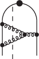
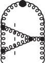
NS $(d_{R})$ real         NS $(d_{V})$ virtual           S $(d_{R})$ real             S $(d_{V})$ virtual

Figure 1: The real and virtual graphs of the type $"(d)"$, contributing to the QCD NLO non-singlet (NS) and singlet (S) splitting functions.

We will discuss in turn these four contributions using the standard formula relating the graphs $\Gamma$ and splitting functions $P$:

$$\Gamma_{qq}(x,\epsilon)=\delta(1-x)+\frac{1}{\epsilon}\biggl{(}\frac{\alpha_{S}}{2\pi}P_{qq}^{LO}(x)+\frac{1}{2}\Bigl{(}\frac{\alpha_{S}}{2\pi}\Bigr{)}^{2}P_{qq}^{NLO}(x)+\dots\biggr{)}+{\cal O}(\epsilon^{-2}).$$

For more details we refer e.g. to [5, 9].

3.1 The virtual non-singlet graph $(d_{V})$ in the NPV scheme

In the NPV scheme the contribution from the non-singlet virtual graph $(d_{V})$ to $\Gamma$ is obtained using the partial results of Ref. [9]: the $T^{(d)V}$ function of eq. (3.152) and the counterterm $V^{(d)V}_{UV}$ of eq. (3.151). The function $T^{(d)V}$ is next evaluated with the help of the library of integrals in the NPV scheme, given in the Appendix. After subtracting $V^{(d)V}_{UV}$ and integrating over the one-particle real phase space we end up with the result

$$\begin{split}\tilde{\Gamma}&{}_{qq}^{(d_{V})}(x,\epsilon)=\left(\frac{\alpha_{S}}{2\pi}\right)^{2}\Big{(}\frac{1}{2}C_{A}C_{F}\Big{)}\biggl{\{}\frac{1}{\epsilon^{2}}P_{qq}(x)\bigl{(}1+\epsilon\ln(1-x)\bigr{)}\tilde{Z}_{d_{V}}-\frac{1}{\epsilon}\frac{1}{2}\frac{1+x}{1-x}\\ &\,+\frac{1}{\epsilon}p_{qq}\biggl{[}I_{0}\bigl{(}2\ln x+2\ln(1-x)\bigr{)}-6I_{1}-\mathrm{Li}_{2}(1-x)+\ln^{2}x-3+\frac{8}{12}{\pi^{2}}\biggr{]}\biggr{\}},\end{split}$$ (7)

where the leading order kernel and renormalization constant are

$$\tilde{Z}_{d_{V}}= \,4I_{0}+2\ln(1-x)+\ln x-\frac{3}{2},$$ (8)

$$P_{qq}(x)= \,p_{qq}+\epsilon(1-x),\;\;\;\;p_{qq}=\frac{1+x^{2}}{1-x}.$$ (9)

3.2 The real non-singlet graph $(d_{R})$ in the NPV scheme

The non-singlet real contribution in the NPV scheme is given in eq. (3.48) of ref. [10]. Here, let us only compare its singular parts with the similar contributions in the PV scheme. The singular terms, i.e. higher-order pole terms and $I$-terms, are in the standard PV prescription ([9] Table 3.10):

$$\frac{P_{qq}(x)}{\epsilon^{2}}-2I_{0}\frac{P_{qq}(x)}{\epsilon}+p_{qq}(x)\Bigl{(}-2I_{1}+4I_{0}+2I_{0}\ln{x}-2I_{0}\ln(1-x)\Bigr{)}$$ (10)

and in the NPV prescription ([10] eq. 3.48):

$$p_{qq}(x)\Bigl{(}2I_{1}+4I_{0}+2I_{0}\ln{x}-2I_{0}\ln(1-x)\Bigr{)}.$$ (11)

Those results are semi-inclusive, i.e. integration over one real momentum, of the generic form $N(\epsilon)\int_{0}^{Q^{2}}d(-q^{2})(-q^{2})^{-1+2\epsilon}$ is not done. Once performed, it will introduce additional $\epsilon$-pole. Here we clearly see the presence of the higher-order $\epsilon$ poles in PV-formula and their absence in NPV-formula, compensated by the change of the coefficient of the $I_{1}$-term.

3.3 Comments on non-singlet $d_{V}$ and $d_{R}$ result in the NPV scheme

Let us compare the NPV results for the non-singlet graphs $(d)$ with the standard PV results available in the literature. Upon combining real and virtual pieces, eq. (3.48) of ref. [10] and eq. (7), we obtain in the NPV scheme

$$\begin{split}\tilde{\Gamma}&{}_{qq}^{(d_{V})+(d_{R})}(x,\epsilon)=\left(\frac{\alpha_{S}}{2\pi}\right)^{2}\Big{(}\frac{1}{2}C_{A}C_{F}\Big{)}\biggl{\{}\frac{1}{\epsilon^{2}}p_{qq}\tilde{Z}_{d_{V}}\\ &\,+\frac{1}{\epsilon}p_{qq}\biggl{[}I_{0}\bigl{(}4\ln x+4\ln(1-x)\bigr{)}+4I_{0}-4I_{1}+3\ln x\ln(1-x)\\ &~{}~{}~{}+\ln^{2}(1-x)+\frac{5}{2}\ln(1-x)+\frac{1}{2}\ln^{2}(x)-\frac{3}{4}\ln(x)-\frac{11}{2}+\frac{1}{2}{\pi^{2}}\bigg{]}\\ &+\frac{1}{\epsilon}\biggl{[}\frac{1}{4}(1+x)\ln(x)-\frac{1}{2}(1-x)+(1-x)\biggl{(}4I_{0}+2\ln(1-x)+\ln x\biggr{)}\biggr{]}\bigg{\}}.\end{split}$$ (12)

This NPV result agrees with the results known from the literature for the standard PV prescription. Namely, the $1/\epsilon^{3}$ and $1/\epsilon^{2}$ $(d_{V})$ and $(d_{R})$ terms are given in Table 3.10 of [9] and the $1/\epsilon$ terms are given in Table 1 of [5] as a sum of real and virtual graphs. We observe, that:

• The $1/\epsilon^{3}$ terms in NPV eq. (12) are absent both in virtual and in real graphs, as we expected. In the standard PV prescription these terms vanish only when real, $(d)^{PV}_{R}$, and virtual, $(d)^{PV}_{V}$, contributions are added.

• The $1/\epsilon^{2}$ terms in NPV eq. (12) are of purely virtual origin and are equal to the sum of the corresponding virtual $(d)^{PV}_{V}$ and real $(d)^{PV}_{R}$ terms in the standard PV prescription. This is a consequence of the absence of $1/\epsilon^{2}$ terms in the real graph (d) in the NPV scheme, see eq. (11).

• The $1/\epsilon$ virtual plus real terms given in NPV eq. (12) agree with the known PV result.

Let us note, that in the NPV scheme there is no dependence on the upper integration limit $\ln Q^{2}$ and no ”artifact” terms $(\ln 4\pi-\gamma_{E})$ are present, in none of the above $(d_{V})$ and $(d_{R})$ contributions. Of course, these ”artifacts” would show up only in the plain MS scheme. If $\overline{\text{MS}}$-like scheme were used, these $(\ln 4\pi-\gamma_{E})$ terms, would be absent anyway. However, the dependence on $\ln Q^{2}$ would still be present (if the PV prescription would have been used).

3.4 The virtual singlet graph $(d_{V})$ in the NPV scheme

Next we turn to the graphs contributing to the singlet splitting function, depicted in Fig. 1. The calculation of the virtual graph proceeds as in the non-singlet case. The counter term can be found e.g. in eq. (3.97) of [9], the corresponding $T^{(d)V}$ is not available in the literature. The renormalized $\Gamma_{gg}^{(d_{V})}$ is then calculated as the bare one minus the counterterm integrated over the one particle phase space:

$$\begin{split}\tilde{\Gamma}&{}_{gg}^{(d_{V})}(x,\epsilon)=\left(\frac{\alpha_{S}}{2\pi}\right)^{2}C_{A}^{2}\frac{1}{2}\biggl{[}\frac{1}{\epsilon^{2}}P_{gg}\bigl{(}1+\epsilon\ln(1-x)\bigr{)}\tilde{Z}_{GS}^{V}\\ &+\frac{1}{\epsilon}P_{gg}\biggl{(}4I_{0}\ln(1-x)+8I_{0}\ln(x)-16I_{1}+4\ln^{2}(x)+12\frac{\pi^{2}}{6}-\frac{134}{9}\biggr{)}-\frac{1}{\epsilon}\frac{1}{3}x\biggr{]},\end{split}$$ (13)

where

$$\tilde{Z}_{GS}^{V}= 12I_{0}+4\ln(1-x)+4\ln(x)-\frac{22}{3},$$ (14)

$$P_{gg}= \frac{(1-x+x^{2})^{2}}{x(1-x)}.$$ (15)

3.5 The real singlet graph $(d_{R})$ in the NPV scheme

In order to complete the calculations we have computed the singlet real graph $(d_{R})$ in the NPV scheme. As in the non-singlet case, the calculation is less complicated than in the standard PV scheme. Due to absence of higher order poles it can be done in four dimensions, leading to

$$\begin{split}\tilde{\Gamma}&{}_{gg}^{(d_{R})}(x,\epsilon)=-\left(\frac{\alpha_{S}}{2\pi}\right)^{2}C_{A}^{2}\frac{1}{2}\frac{1}{\epsilon}\biggl{[}P_{gg}\biggl{(}-4I_{1}-8I_{0}+4I_{0}\ln(1-x)-4I_{0}\ln(x)\\ &+2\ln^{2}(1-x)+2\ln^{2}(x)-4\ln(x)\ln(1-x)-8\ln(1-x)+\frac{11}{3}\ln(x)+2\frac{\pi^{2}}{6}+4\biggr{)}\\ &+\ln(x)\Bigl{(}\frac{11}{3}x^{2}+\frac{23}{6}x+\frac{23}{6}+\frac{11}{3x}\Bigr{)}-\frac{22}{3}x^{2}+\frac{24}{3}x-\frac{25}{3}+\frac{22}{3x}\biggr{]}.\end{split}$$ (16)

3.6 Comments on singlet $d_{V}$ and $d_{R}$ result in the NPV scheme

Now we compare the singlet NPV results with the corresponding PV results from the literature. Having added the real and virtual graphs in the NPV prescription, eqs. (16) and (13), we obtain

$$\begin{split}\tilde{\Gamma}&{}_{gg}^{(d_{V})+(d_{R})}(x,\epsilon)=\left(\frac{\alpha_{S}}{2\pi}\right)^{2}C_{A}^{2}\frac{1}{2}\biggl{\{}\frac{1}{\epsilon^{2}}P_{gg}\tilde{Z}_{GS}^{V}\\ &+\frac{1}{\epsilon}\biggl{[}P_{gg}\biggl{(}12I_{0}\ln(x)+12I_{0}\ln(1-x)+8I_{0}-12I_{1}+2\ln^{2}(1-x)\\ &+2\ln^{2}(x)+8\ln(x)\ln(1-x)-\frac{11}{3}\ln(x)+\frac{2}{3}\ln(1-x)+10\frac{\pi^{2}}{6}-\frac{170}{9}\biggr{)}\\ &-\Bigl{(}\frac{11}{3}x^{2}+\frac{23}{6}x+\frac{23}{6}+\frac{11}{3x}\Bigr{)}\ln(x)+\frac{22}{3}x^{2}-\frac{25}{3}x+\frac{25}{3}-\frac{22}{3x}\biggr{]}\biggr{\}}.\end{split}$$ (17)

This NPV $(d_{V})+(d_{R})$ result agrees with the PV results from the literature: in particular the $1/\epsilon^{3}$ and $1/\epsilon^{2}$ terms given (separately for real and virtual graphs) in Table 3.12 of ref. [9] and the $1/\epsilon$ terms given (only as a sum of real and virtual graphs) in Table 4 column (cd) of ref. [6]. The detailed comments to this comparison are identical as for the non-singlet comparison of Sect. 3.3.

Since the other contributions to the NLO $P_{qq}$ and $P_{gg}$ splitting functions remain unchanged while moving from the PV to NPV prescription, this completes the re-calculation of the NLO $P_{qq}$ and $P_{gg}$ splitting functions and demonstrates that the final results are identical in both schemes.

4 Summary

We proposed an extension of the use of the PV prescription in the light-cone gauge, and we applied it to all the singularities in the plus component of the integration momentum. We have shown that in the new NPV prescription the NLO splitting functions, both non-singlet $P_{qq}$ and singlet $P_{gg}$, are reproduced correctly. The differences with respect to the PV scheme are present in partial results of subset of four graphs, labelled $"(d)"$. The $1/\epsilon^{3}$ poles, present in PV, are now replaced by $(1/\epsilon)\ln^{2}\delta$ etc. Therefore, the calculations are easier, in particular the real graphs, now free of $1/\epsilon^{3}$ and $1/\epsilon^{2}$ poles, can be calculated in four dimensions and are usable for the Monte Carlo stochastic simulations, cf. eg. [19]. The higher order poles cancel separately for real and for virtual components and neither real nor virtual contribution depend on the scale $Q$ of the hard process. This is not true for the standard prescription – in that case only the sum of real and virtual terms is independent of $Q$. The drawback of the NPV prescription is that the non-axial integrals entering calculations start to depend on the auxiliary vector $n$ and become more complicated.

Appendix A Three-point integrals in NPV scheme

We present the complete list of three-point integrals relevant for the calculations of the NLO splitting functions which are modified in NPV with respect to the standard PV prescription. The integrals are valid for the specific kinematics: $p^{2}=0,\;(p-q)^{2}=k^{2}=0,\;q^{2}<0$. The complete list of integrals in the PV prescription can be found in Appendix A of [9].

$$\{J_{3}^{A},\,J_{3}^{A\mu},\,J_{3}^{A\mu\nu}\}=\int\frac{d^{m}l}{(2\pi)^{m}}\frac{\{1,\,l^{\mu},\,l^{\mu}l^{\nu}\}}{l^{2}(p-l)^{2}(q-l)^{2}}\frac{1}{nl}.$$ (18)

The Feynman integrals, $J_{3}$, are similar but without the $1/(nl)$ term and $J_{3}^{n3}=J_{3}^{\mu\nu\rho}n_{\mu}n_{\nu}n_{\rho}$ and so on. The normalization $Q_{\epsilon}$, common to all the integrals, is defined as

$$Q_{\epsilon}(r)=i\frac{1}{(4\pi)^{2+\epsilon}}\Gamma(1-\epsilon)\frac{(-r^{2})^{\epsilon}}{(\mu_{R}^{2})^{\epsilon}}.$$ (19)

Feynman integrals are defined as:

$$J_{3}^{\alpha\beta}(q,p)= \frac{Q_{\epsilon}(q)}{q^{2}}\Bigl{(}R_{3}p^{\alpha}p^{\beta}+R_{4}q^{\alpha}q^{\beta}+R_{5}(q^{\alpha}p^{\beta}+p^{\alpha}q^{\beta})+R_{6}q^{2}g^{\alpha\beta}\Bigr{)},$$ (20)

$$J_{3}^{\alpha}(q,p)= \frac{Q_{\epsilon}(q)}{q^{2}}\Bigl{(}R_{1}p^{\alpha}+R_{2}q^{\alpha}\Bigr{)},$$ (21)

$$J_{3}^{n3}(q,p)= -\frac{Q_{\epsilon}(q)}{q^{2}}(pn)^{3}(N_{3}-R_{0}),$$ (22)

$$J_{3}^{n2}(q,p)= -\frac{Q_{\epsilon}(q)}{q^{2}}(pn)^{2}(N_{2}-R_{0}),$$ (23)

$$J_{3}^{n1}(q,p)= -\frac{Q_{\epsilon}(q)}{q^{2}}(pn)^{1}(N_{1}-R_{0}),$$ (24)

$$J_{3}(q,p)= \frac{Q_{\epsilon}(q)}{q^{2}}R_{0}.$$ (25)

Axial integrals are defined as:

$$J_{3}^{A\alpha}(q,p)= \frac{Q_{\epsilon}(q)}{q^{2}pn}\Bigl{(}S_{1}p^{\alpha}+S_{2}q^{\alpha}+\frac{1}{2q^{2}qn}S_{3}n^{\alpha}\Bigr{)},$$ (26)

$$J_{3}^{A}(q,p)= \frac{Q_{\epsilon}(q)}{q^{2}pn}S_{0},$$ (27)

$$J_{3}^{A}(-q,k)= \frac{Q_{\epsilon}(q)}{q^{2}kn}U_{0}.$$ (28)

Functions $N$ and the modified in the NPV scheme functions ${R^{NPV}},\,{S^{NPV}}$ and ${U^{NPV}}$ read:

$$R^{NPV}_{3}= R^{NPV}_{1}-\frac{1}{\epsilon}+3,$$ (29)

$$R^{NPV}_{1}= R^{NPV}_{0}-\frac{2}{\epsilon}+4,$$ (30)

$$R^{NPV}_{0}= -\Bigl{(}-2\frac{I_{0}}{\epsilon}-\frac{1}{\epsilon}\ln(1-x)-4I_{1}+2I_{0}\ln(1-x)+\frac{\ln^{2}(1-x)}{2}\Bigr{)},$$ (31)

$$U^{NPV}_{0}= -\Bigl{(}-\frac{3I_{0}}{\epsilon}-\frac{3}{\epsilon}\ln(1-x)+\frac{1}{\epsilon}\ln(x)-5I_{1}+2I_{0}\ln(1-x)+I_{0}\ln(x)$$

$$-\frac{1}{2}\ln^{2}(1-x)-2\mathrm{Li}_{2}(1-x)+\frac{1}{2}\ln^{2}(x)+5\frac{\pi^{2}}{6}\Bigr{)},$$ (32)

$$S^{NPV}_{0}= \frac{3I_{0}}{\epsilon}+\frac{1}{\epsilon}\ln(1-x)-\frac{1}{\epsilon}\ln(x)+5I_{1}-2I_{0}\ln(1-x)-I_{0}\ln(x)$$

$$-\frac{1}{2}\ln^{2}(x)-\frac{1}{2}\ln^{2}(1-x)-2\mathrm{Li}_{2}(1-x)-\frac{\pi^{2}}{6},$$ (33)

$$S^{NPV}_{1}= \frac{2I_{0}}{\epsilon}+\frac{1}{\epsilon}\ln(1-x)+4I_{1}-2I_{0}\ln(1-x)-\frac{1}{2}\ln^{2}(1-x)$$

$$+\frac{1}{\epsilon}\frac{x}{(1-x)}\ln(x)+\frac{x}{(1-x)}\mathrm{Li}_{2}(1-x),$$ (34)

$$N_{3}= -\frac{1}{\epsilon}\Bigl{(}\frac{x^{3}}{3}+\frac{x^{2}}{2}+{x}-\frac{11}{3}\Bigr{)}+\Bigr{(}\frac{13}{18}x^{3}+\frac{4}{3}x^{2}+\frac{11}{3}x-\frac{85}{9}\Bigr{)},$$ (35)

$$N_{2}= -\frac{1}{\epsilon}\Bigr{(}\frac{x^{2}}{2}+{x-3}\Bigr{)}+(x^{2}+3x-7),$$ (36)

$$N_{1}= -\frac{x-2}{\epsilon}+2(x-2).$$ (37)

The remaining $R,\,S$ and $U$ functions are identical in the PV and NPV schemes and can be found in [9], see also footnote 3.

References

- [1] M. Skrzypek, S. Jadach, A. Kusina, W. Placzek, M. Slawinska, et al., Fully NLO Parton Shower in QCD, Acta Phys.Polon. B42 (2011) 2433–2443. arXiv:1111.5368, doi:10.5506/APhysPolB.42.2433.
- [2] S. Jadach, M. Jezabek, A. Kusina, W. Placzek, M. Skrzypek, NLO corrections to hard process in QCD shower – proof of concept, Acta Phys.Polon. B43 (2012) 2067. arXiv:1209.4291.
- [3] S. Jadach, A. Kusina, W. Placzek, M. Skrzypek, M. Slawinska, Inclusion of the QCD next-to-leading order corrections in the quark-gluon Monte Carlo shower, Phys.Rev. D87 (2013) 034029. arXiv:1103.5015, doi:10.1103/PhysRevD.87.034029.
- [4] E. Oliveira, A. Martin, M. Ryskin, Treatment of the infrared contribution: NLO QED evolution as a pedagogic example, Eur.Phys.J. C73 (2013) 2534. arXiv:1305.6406, doi:10.1140/epjc/s10052-013-2534-3.
- [5] G. Curci, W. Furmanski, R. Petronzio, Evolution of parton densities beyond leading order: the non-singlet case, Nucl. Phys. B175 (1980) 27.
- [6] R. K. Ellis, W. Vogelsang, The evolution of parton distributions beyond leading order: the singlet casearXiv:hep-ph/9602356.
- [7] G. Heinrich, Z. Kunszt, Two-loop anomalous dimension in light-cone gauge with Mandelstam-Leibbrandt prescription, Nucl. Phys. B519 (1998) 405–432. arXiv:hep-ph/9708334, doi:10.1016/S0550-3213(98)00089-3.
- [8] A. Bassetto, G. Heinrich, Z. Kunszt, W. Vogelsang, The light-cone gauge and the calculation of the two-loop splitting functions, Phys. Rev. D58 (1998) 094020. arXiv:hep-ph/9805283, doi:10.1103/PhysRevD.58.094020.
-
[9]
G. Heinrich, Improved
techniques to calculate two-loop anomalous dimensions in qcd, Ph.D. thesis,
Swiss Federal Institute of Technology, Zurich (1998).
URL http://dx.doi.org/10.3929/ethz-a-001935934 - [10] S. Jadach, A. Kusina, M. Skrzypek, M. Slawinska, Two real parton contributions to non-singlet kernels for exclusive QCD DGLAP evolution, JHEP 08 (2011) 012. arXiv:1102.5083, doi:10.1007/JHEP08(2011)012.
- [11] S. Mandelstam, Light Cone Superspace and the Ultraviolet Finiteness of the N=4 Model, Nucl.Phys. B213 (1983) 149–168. doi:10.1016/0550-3213(83)90179-7.
- [12] G. Leibbrandt, The Light Cone Gauge in Yang-Mills Theory, Phys.Rev. D29 (1984) 1699. doi:10.1103/PhysRevD.29.1699.
- [13] A. Suzuki, A. Schmidt, The light cone gauge without prescriptions, Prog.Theor.Phys. 103 (2000) 1011–1019. arXiv:hep-th/9904004, doi:10.1143/PTP.103.1011.
- [14] Z. Bern, L. J. Dixon, D. A. Kosower, Two-loop g gg splitting amplitudes in QCD, JHEP 0408 (2004) 012. arXiv:hep-ph/0404293, doi:10.1088/1126-6708/2004/08/012.
- [15] G. Nardelli, R. Soldati, Euclidean Wilson Loop and Axial Gauge, Int.J.Mod.Phys. A5 (1990) 3171–3192. doi:10.1142/S0217751X90002142.
- [16] R. K. Ellis, H. Georgi, M. Machacek, H. D. Politzer, G. G. Ross, Factorization and the parton model in qcd, Phys. Lett. B78 (1978) 281.
- [17] G. Heinrich, G. Leibbrandt, Split dimensional regularization for the Coulomb gauge at two loops, Nucl.Phys. B575 (2000) 359–382. arXiv:hep-th/9911211, doi:10.1016/S0550-3213(00)00078-X.
- [18] W. Furmanski, R. Petronzio, Singlet parton densities beyond leading order, Phys. Lett. B97 (1980) 437.
- [19] S. Jadach, A. Kusina, W. Placzek, M. Skrzypek, NLO corrections in the initial-state parton shower Monte Carlo, arXiv:1310.6090.