YITP-13-123 KUNS-2470

Emergent bubbling geometries in the plane wave matrix model

Yuhma Asano¹⁾, Goro Ishiki^1),2), Takashi Okada^1),2),3) and Shinji Shimasaki¹⁾

¹⁾ Department of Physics, Kyoto University
Kyoto, 606-8502, Japan

²⁾ Yukawa Institute for Theoretical Physics, Kyoto University
Kyoto, 606-8502, Japan

³⁾ Kavli Institute for Theoretical Physics, UCSB
Santa Barbara CA 93106

The gravity dual geometry of the plane wave matrix model is given by the bubbling geometry in the type IIA supergravity, which is described by an axially symmetric electrostatic system. We study a quarter BPS sector of the plane wave matrix model in terms of the localization method and show that this sector can be mapped to a one-dimensional interacting Fermi gas system. We find that the mean-field density of the Fermi gas can be identified with the charge density in the electrostatic system in the gravity side. We also find that the scaling limits in which the dual geometry reduces to the D2-brane or NS5-brane geometry are given as the free limit or the strongly coupled limit of the Fermi gas system, respectively. We reproduce the radii of $S^{5}$’s in these geometries by solving the Fermi gas model in the corresponding limits.

1 Introduction

The gauge/string duality is a conjectured equivalence between strongly coupled gauge field theories and weakly coupled perturbative string theories [1, 2, 3]. One of the most important problems in understanding this duality is how the space-time geometry described in the string theory emerges in the framework of the corresponding gauge theory. If the duality is true, the background space-time in the string theory should emerge in the strong coupling region of the gauge theories, although it may not be apparent in the weak coupling region. See [4, 5, 6, 7, 8] for recent developments on the emergent space-time.

In this paper, we analyze a one-dimensional gauge theory in the strong coupling region and study the emergent phenomena of geometries. The theory we consider is a matrix quantum mechanics called the plane wave matrix model (PWMM), which was proposed as a fundamental formulation of the M-theory on the pp-wave background in the light-cone frame [9]. PWMM has $SU(2|4)$ symmetry, which consists of $R\times SO(3)\times SO(6)$ bosonic symmetry and 16 supersymmetries. PWMM is a mass deformation of the BFSS matrix model [10] and has many discrete vacua given by fuzzy spheres that are labeled by representations of the $SU(2)$ Lie algebra. In this paper, we consider the case where the representation is given by a direct sum of the same irreducible representations. In this case, the vacua are labeled by two integers $(N_{2},N_{5})$, where $N_{5}$ is the dimension of the irreducible representation and $N_{2}$ is the multiplicity.

For the theory around each vacuum of PWMM, a corresponding gravity dual geometry in the type IIA superstring theory was constructed in [12, 11] (also studied in [13] in the Polchinski-Strassler approximation). The geometry is called the bubbling geometry and characterized by fermionic droplets on a certain two-dimensional subspace of the space-time, which define a boundary condition of the solution. By a simple change of variables, the geometry can be equivalently characterized by a three-dimensional axially symmetric electrostatic system with some conducting disks (see the next section). The geometry locally has a topology of $R\times S^{2}\times S^{5}\times{\cal M}_{e}$, where ${\cal M}_{e}\sim R^{2}$ corresponds to the space on which the electrostatic system is defined. For theories around the above mentioned vacua labeled by two integers $(N_{2},N_{5})$, the gravity dual geometries were studied in detail in [14]. The integers, $N_{2}$ and $N_{5}$, are interpreted as the D2-brane and NS5-brane charges in the dual geometries, respectively [15].

In order to see the emergence of this geometry in PWMM, we consider a complex scalar field $\phi(t)\sim X_{4}(t)+i(X_{9}(t)\sin t+X_{10}(t)\cos t)$, where $X_{4}$ is one of $SO(3)$ scalar fields, $X_{9,10}$ are $SO(6)$ scalars and $t$ is the time coordinate. We consider a quarter BPS sector of PWMM which consists of correlators of only $\phi$’s. Since $\phi$ has two real degrees of freedom, it should describe a two-dimensional surface on the gravity dual geometry. Let ${\cal M}_{\phi}$ be a two-dimensional subspace in the bubbling geometry described by $\phi$. For a fixed $t$, insertions of the field $\phi(t)$ in the path integral break the original $R\times SO(3)\times SO(6)$ symmetry to $SO(2)\times SO(5)$, which is the symmetry of $S^{2}\times S^{5}$ with a marked point. Hence, ${\cal M}_{\phi}$ is expected to be fibered on the marked point on $S^{2}\times S^{5}$. From the original symmetry, however, ${\cal M}_{\phi}$ should exists everywhere on $R\times S^{2}\times S^{5}$, so that the topology of the total space should be locally given by $R\times S^{2}\times S^{5}\times{\cal M}_{\phi}$. Thus, the subspace ${\cal M}_{\phi}$ can naturally be identified with the space ${\cal M}_{e}$ of the electrostatic problem.

Recently, the localization method, which makes exact computations possible for some supersymmetric operators [17, 16], was applied to the above sector of $\phi$ [18]. In this paper, using this result, we first show that this sector can be mapped to a one-dimensional interacting Fermi gas system. We then find that in a strong coupling region, the mean-field density of the Fermi particles satisfies the same integral equation as the charge density which appears in the electrostatic system in the gravity side. Thus we identify the mean-field density with the charge density. Since the charge density ultimately determines the gravity dual solution, this identification makes it possible to reconstruct the bubbling geometry based on the gauge theory.

This situation is very similar to the case of the bubbling geometries in the type IIB supergravity which has $R\times SO(4)\times SO(4)$ symmetry and 16 supersymmetries [12]. These geometries correspond to a sector of the half BPS operators in the ${\cal N}=4$ Super Yang-Mills theory (SYM) on $R\times S^{3}$ that consists of zero modes on $S^{3}$ of a complex scalar field $Z=\Phi_{4}+i\Phi_{5}$. This sector can also be mapped to a one-dimensional fermionic system and its phase space density can be identified with the the droplets in the gravity side [19, 20].

In the case of ${\cal N}=4$ SYM, the sector of $Z$ is protected by the non-renormalization theorem, so it does not depend on the coupling constant [21, 22]. In our case, however, the sector we consider in this paper depends on various tunable parameters such as the coupling constant and the parameters $(N_{2},N_{5})$ of the vacua. Hence we can also consider some scaling limits for these parameters. The gravity dual of PWMM has two interesting scaling limits which we call the D2-brane limit and the NS5-brane limit in this paper [11, 14]. In the D2-brane limit, the NS5-brane charges decouple and only the D2-brane charge is left in the geometry. The geometry asymptotically becomes the D2-brane solution. In the same manner, the NS5-brane limit sends the geometry to the NS5-brane solution. In this paper, We show that the D2-brane and the NS5-brane limits are realized on the gauge theory side as the free and strongly coupled limits of the Fermi gas system, respectively. In these limits, we solve the Fermi gas system at the planar level and reproduce the radii of the $S^{5}$’s in the gravity side. In particular, the $S^{5}$ corresponds to the spatial worldvolume of fivebranes in the case of the NS5-brane limit and its radius has been known to be proportional to $\lambda^{1/4}$ in the string unit, where $\lambda$ is the ’t Hooft coupling in PWMM[15]. Our gauge theory result reproduces this behavior and hence gives a strong evidence for the description of fivebranes in PWMM proposed in [15].

This paper is organized as follows. In section 2, we review PWMM and the result of the localization [18]. In section 3, we review the gravity dual of PWMM. In section 4, we first map the matrix integral obtained through the localization to an interacting Fermi gas system. Then we identify the mean-field density with the charge density. We also perform various consistency checks of this identification. Section 5 is devoted to summary and discussion.

2 Plane wave matrix model

In this section, we review PWMM [9] and the result of the localization obtained in [18]. We use the same notation as in [18]. The action of PWMM is written in terms of the ten-dimensional notation as,

$$S =\frac{1}{g^{2}}\int d\tau\mathrm{Tr}\Bigl{(}\frac{1}{4}F_{MN}F^{MN}+\frac{m^{2}}{8}X_{m}X^{m}+\frac{i}{2}\Psi\Gamma^{M}D_{M}\Psi\Bigr{)},$$ (2.1)

where the time direction is assumed to be the Euclidean signature and

$$F_{1M} =D_{1}X_{M}=\partial_{1}X_{M}-i[X_{1},X_{M}]\quad(M\neq 1),$$

$$F_{a^{\prime}b^{\prime}} =m\varepsilon_{a^{\prime}b^{\prime}c^{\prime}}X_{c^{\prime}}-i[X_{a^{\prime}},X_{b^{\prime}}],\quad F_{a^{\prime}m}=D_{a^{\prime}}X_{m}=-i[X_{a^{\prime}},X_{m}],\quad F_{mn}=-i[X_{m},X_{n}],$$

$$D_{1}\Psi =\partial_{1}\Psi-i[X_{1},\Psi],\quad D_{a^{\prime}}\Psi=\frac{m}{8}\varepsilon_{a^{\prime}b^{\prime}c^{\prime}}\Gamma^{b^{\prime}c^{\prime}}\Psi-i[X_{a^{\prime}},\Psi],\quad D_{m}\Psi=-i[X_{m},\Psi].$$ (2.2)

The range of indices are $M,N=1,\cdots,10$, $a^{\prime},b^{\prime}=2,3,4$ and $m,n=5,\cdots,10$. $X_{1}$ is the one-dimensional gauge field, $X_{a^{\prime}}$ and $X_{m}$ are $SO(3)$ and $SO(6)$ scalars and $\Psi$ is a fermionic field with 16 components. We put $m=2$ for the mass parameter in the following. The $m$ dependence can be recovered anytime by the dimensional analysis.

The vacuum of PWMM is given by the fuzzy sphere, namely,

$$X_{a}=-2L_{a},\;\;(a=2,3,4)$$ (2.3)

and all the other matrices are zero. Here $L_{a}$ are representation matrices of $SU(2)$ generators. For any representation of $SU(2)$, (2.3) gives a classical vacuum of PWMM which preserves 16 supersymmetries. The representation of $L_{a}$ is reducible in general and it can be decomposed as

$$L_{a}=\bigoplus_{s=1}^{\Lambda}({\bf 1}_{N_{2}^{(s)}}\otimes L_{a}^{[N_{5}^{(s)}]}),$$ (2.4)

where $L_{a}^{[N]}$ are $SU(2)$ generators in the $N$ dimensional irreducible representation. $N_{2}^{(s)}$ denote the multiplicities of the irreducible representations and $\sum_{s}N_{2}^{(s)}N_{5}^{(s)}$ must be equal to the matrix size in PWMM. The notation for $N_{2}^{(s)}$ and $N_{5}^{(s)}$ indicates that they correspond to membrane and 5-brane charges in M-theory, respectively [15].

In order to define the path integral of PWMM, one has to specify the boundary conditions at $\tau\rightarrow\pm\infty$. To study the theory around a fixed vacuum of PWMM, the appropriate boundary condition is such that all fields approach to the vacuum configuration at the both infinities. When the multiplicities are sufficiently large compared to the other parameters, the instanton effects can be ignored, so that the path integral with this boundary condition defines the theory around the fixed vacuum.

Let us define a complex scalar field,

$$\phi(\tau)=2(-X_{4}(\tau)+\sinh\tau X_{9}(\tau)+i\cosh\tau X_{10}(\tau)).$$ (2.5)

When $\tau$ is Wick-rotated to the Lorentzian signature, the real and the imaginary parts of $\phi$ are given by a $SO(3)$ scalar and $SO(6)$ scalars, respectively, as introduced in the previous section. On the other hand, in another Lorentzian signature where the $X_{10}$ direction is Wick-rotated as in [16], four supersymmetries which leave $\phi$ invariant were constructed [18]. See appendix B for these supersymmetries.

For the theory around each vacuum of PWMM, one can compute the correlators made of $\phi$’s by Wick-rotating $X_{10}$ and applying the localization with the above mentioned boundary conditions [18]. The result of the localization in [18] is summarized below. The following equality holds,

$$\langle\prod_{a}{\rm Tr}f_{a}(\phi(\tau_{a}))\rangle=\langle\prod_{a}{\rm Tr}f_{a}(4L_{4}+2iM)\rangle_{MM},$$ (2.6)

where $f_{a}$ are arbitrary smooth functions. On the left-hand side of (2.6), the expectation value is taken in the theory around the vacuum (2.4) in PWMM. On the right-hand side of (2.6), $M$ is a Hermitian matrix with the following block structure,

$$M=\bigoplus_{s=1}^{\Lambda}(M_{s}\otimes{\bf 1}_{N_{5}^{(s)}}),$$ (2.7)

where $M_{s}$ $(s=1,\cdots,\Lambda)$ are $N_{2}^{(s)}\times N_{2}^{(s)}$ Hermitian matrices. $\langle\cdots\rangle_{MM}$ stands for an expectation value with respect to the following partition function,

$$Z_{{\cal R}}=\int\prod_{s=-\Lambda/2}^{\Lambda/2}\prod_{i=1}^{N_{2}^{(s)}}dq_{si}Z_{\rm 1-loop}({\cal R},\{q_{si}\})e^{-\frac{2}{g^{2}}\sum_{s}\sum_{i}N_{5}^{(s)}q_{si}^{2}},$$ (2.8)

where ${\cal R}$ denotes the representation of (2.4), $q_{si}$ are eigenvalues of $M_{s}$ and

$$Z_{\rm 1-loop}=\prod_{s,t=-\Lambda/2}^{\Lambda/2}\prod_{J}\prod_{i=1}^{N_{2}^{(s)}}\prod_{j=1}^{N_{2}^{(t)}}{\phantom{\prod}}^{\prime}\left[\frac{\{(2J+2)^{2}+(q_{si}-q_{tj})^{2}\}\{(2J)^{2}+(q_{si}-q_{tj})^{2}\}}{\{(2J+1)^{2}+(q_{si}-q_{tj})^{2}\}^{2}}\right]^{\frac{1}{2}}.$$ (2.9)

In (2.9), the product of $J$ runs from $|N_{5}^{(s)}-N_{5}^{(t)}|/2$ to $(N_{5}^{(s)}+N_{5}^{(t)})/2-1$. And $\prod^{\prime}$ means that the second factor in the numerator with $s=t$, $J=0$ and $i=j$ is not included in the product.

Note that (2.6) implies that the left hand side of (2.6) does not depend on the positions $\{\tau_{a}\}$ of the operators. This follows from the supersymmetry Ward identity in PWMM. As shown in appendix A, there exists a fermionic matrix $\Psi_{1}$ in PWMM such that its variation under the supersymmetry is proportional to $D_{1}\phi$. Then, it follows from the Ward identity that

$$0=\delta_{s}\langle{\rm Tr}(\Psi_{1}\phi^{m})(\tau)\cdots\rangle=\frac{1}{m+1}\langle{\rm Tr}(D_{1}\phi^{m+1})(\tau)\cdots\rangle=\frac{1}{m+1}\frac{\partial}{\partial\tau}\langle{\rm Tr}(\phi^{m+1})(\tau)\cdots\rangle,$$ (2.10)

where $\cdots$ stands for operators made of $\phi$’s only. Hence, they are indeed independent of the positions. One can also check this easily by a perturbative calculation around each vacuum.

In this paper, we consider the case of $\Lambda=1$. In this case, (2.8) is just a one matrix model,

$$Z= \int\prod_{i}dq_{i}\prod_{J=0}^{N_{5}-1}\prod_{i>j}^{N_{2}}\frac{\{(2J+2)^{2}+(q_{i}-q_{j})^{2}\}\{(2J)^{2}+(q_{i}-q_{j})^{2}\}}{\{(2J+1)^{2}+(q_{i}-q_{j})^{2}\}^{2}}e^{-\frac{2N_{5}}{g^{2}}\sum_{i}q_{i}^{2}}.$$ (2.11)

When $N_{5}=1$, (2.11) takes the same form as the partition function of the six-dimensional version of the IKKT matrix model with a suitable regularization [33, 34].

3 Gravity dual of PWMM

In this section, we review the dual geometry for PWMM. The gravity duals for the gauge theories with $SU(2|4)$ symmetry, which consist of PWMM, ${\cal N}=8$ SYM on $R\times S^{2}$ and ${\cal N}=4$ SYM on $R\times S^{3}/Z_{k}$, were constructed by Lin and Maldacena [11]. They assumed the $SU(2|4)$ symmetric ansatz and then showed that finding the classical solutions is reduced to the problem of finding axially symmetric solutions to the 3d Laplace equation with appropriate boundary conditions given by parallel charged conducting disks and a background potential.

3.1 Dual geometry of PWMM

The supergravity solutions dual to the $SU(2|4)$ symmetric theories are given by

$$ds_{10}^{2} =\left(\frac{\ddot{V}-2\dot{V}}{-V^{\prime\prime}}\right)^{1/2}\left\{-4\frac{\ddot{V}}{\ddot{V}-2\dot{V}}dt^{2}-2\frac{V^{\prime\prime}}{\dot{V}}(dr^{2}+dz^{2})+4d\Omega_{5}^{2}+2\frac{V^{\prime\prime}\dot{V}}{\Delta}d\Omega_{2}^{2}\right\},$$

$$C_{1} =-\frac{(\dot{V}^{2})^{\prime}}{\ddot{V}-2\dot{V}}dt,\;\;\;C_{3}=-4\frac{\dot{V}^{2}V^{\prime\prime}}{\Delta}dt\wedge d\Omega_{2},$$

$$B_{2} =\left(\frac{(\dot{V}^{2})^{\prime}}{\Delta}+2z\right)d\Omega_{2},\;\;\;e^{4\Phi}=\frac{4(\ddot{V}-2\dot{V})^{3}}{-V^{\prime\prime}\dot{V}^{2}\Delta^{2}},$$ (3.1)

where $\Delta=(\ddot{V}-2\dot{V})V^{\prime\prime}-(\dot{V}^{\prime})^{2}$ and the dots and primes indicate $\frac{\partial}{\partial\log r}$ and $\frac{\partial}{\partial z}$, respectively. Note that the solution is written in terms of a single function $V(r,z)$. The Killing spinor equations in the supergravity are reduced to the Laplace equation for $V$ in a three-dimensional axially symmetric electrostatic system, where the coordinates for the axial and the transverse directions are given by $z$ and $r$, respectively. Thus $V$ can be regarded as an electrostatic potential in this system.

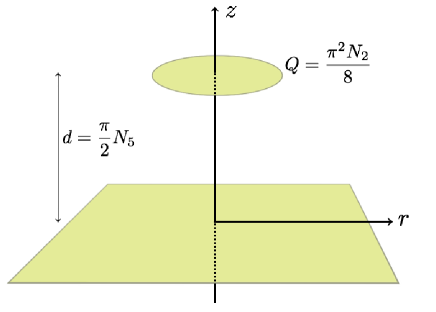
Figure 1: The electrostatic system for PWMM around the vacua labeled by $(N_{2},N_{5})$.

The electrostatic system for the dual geometry of PWMM involves an infinite conducting surface at $z=0$ and only the region $z\geq 0$ is relevant. See Fig. 1. The positivity of the metric requires the presence of the background potential of the form $V_{0}(r^{2}z-\frac{2}{3}z^{3})$, where $V_{0}$ is a constant. In addition to the infinite surface, the system has some finite conducting disks. The positions and charges of these disks are related to the parameters of the vacua in PWMM. For the gravity dual of PWMM around the vacuum (2.3) with (2.4), the system has $\Lambda$ disks each of which has the charge $\pi^{2}N_{2}^{(s)}/8$ and resides at the position $z=\pi N_{5}^{(s)}/2$, where $s=1,\cdots,\Lambda$. (The radii of the disks are not free parameters. The regularity of the gravity solution demands that the charge density on a finite disk vanishes at the edge, which relates the radius of the disk to the charge.) The solution $V(r,z)$ of the Laplace equation in this electrostatic system determines the gravity solution (3.1) that is dual to the PWMM around the vacuum (2.3) with (2.4). In this geometry, $N_{5}^{(s)}$ and $N_{2}^{(s)}$ correspond to the charges of NS5-branes and D2-branes, respectively, and $s=1,\cdots,\Lambda$ labels independent cycles with the flux of the branes.

The gravity solution that corresponds to the vacuum with $\Lambda=1$ in PWMM was studied in detail in [14]. The electrostatic system associated with this solution consists of one infinite conducting plate at $z=0$ and another finite conducting disk at $z=d>0$ with radius $R$ and charge $Q$. The background potential is given by $V_{0}(r^{2}z-\frac{2}{3}z^{3})$. $Q$ and $d$ are related to the brane charges as $N_{5}=2d/\pi$ and $N_{2}=8Q/\pi^{2}$. By solving the Laplace equation with these boundary conditions, one can determine the potential as

$$V_{PWMM}(r,z) =V_{0}\left(r^{2}z-\frac{2}{3}z^{3}\right)+V_{0}R^{3}\phi_{\kappa}(r/R,z/R),$$ (3.2)

where $\kappa\equiv d/R$ and $\phi_{\kappa}(r,z)$ is given by

$$\phi_{\kappa}(r,z) =\frac{\beta(\kappa)}{\pi}\int^{1}_{-1}dt\left(-\frac{1}{\sqrt{r^{2}+(z+\kappa+it)^{2}}}+\frac{1}{\sqrt{r^{2}+(z-\kappa+it)^{2}}}\right)f_{\kappa}(t).$$ (3.3)

Here $\beta(\kappa)$ is given in terms of $f^{(n)}_{\kappa}(t)$ defined in appendix A as

$$\beta(\kappa) \equiv 2\kappa\frac{f^{(2)}_{\kappa}(1)}{f^{(0)}_{\kappa}(1)},$$ (3.4)

and $f_{\kappa}(t)$ is the solution to the Fredholm integral equation of the second kind,

$$f_{\kappa}(x)-\int_{-1}^{1}dyK_{\kappa}(x,y)f_{\kappa}(y)=1-\frac{f^{(0)}_{\kappa}(1)}{f^{(2)}_{\kappa}(1)}x^{2}$$ (3.5)

with kernel

$$K_{\kappa}(x,y)=\frac{1}{\pi}\frac{2\kappa}{4\kappa^{2}+(x-y)^{2}}.$$ (3.6)

The equation (3.5) is solved by

$$f_{\kappa}(t)=f^{(0)}_{\kappa}(t)-\frac{2\kappa}{\beta(\kappa)}f^{(2)}_{\kappa}(t)=f^{(0)}_{\kappa}(t)-\frac{f^{(0)}_{\kappa}(1)}{f^{(2)}_{\kappa}(1)}f^{(2)}_{\kappa}(t).$$ (3.7)

The charge density $\sigma_{\kappa}(r)$ for the radial direction on the disk is related to $f_{\kappa}(t)$ as

$$\sigma_{\kappa}(r)=-\frac{\beta(\kappa)}{\pi^{2}}\int_{r}^{1}dt\frac{f^{\prime}_{\kappa}(t)}{\sqrt{t^{2}-r^{2}}},\;\;\;\;f_{\kappa}(t)=\frac{2\pi}{\beta(\kappa)}\int_{t}^{1}dr\frac{r\sigma_{\kappa}(r)}{\sqrt{r^{2}-t^{2}}}.$$ (3.8)

From this relation, one can interpret $f_{\kappa}(t)$ as the charge density projected onto a diameter of the disk. The radius of the disk is related to the charge as

$$Q=q(\kappa)V_{0}R^{4},\;\;\;\;q(\kappa)=\frac{\beta(\kappa)}{\pi}\int_{-1}^{1}dtf_{\kappa}(t).$$ (3.9)

The disk radius is related to the radius of $S^{5}$ at the edge of the disk as

$$R=\frac{R^{2}_{S^{5}}}{4\alpha^{\prime}}.$$ (3.10)

One can easily check this by using the Laplace equation to rewrite $V^{\prime\prime}$ and note that $\dot{V}=0$ on the disk.

The parameters of the electrostatic problem were identified with the parameters in PWMM as [11, 14]

$$Q=\frac{\pi^{2}N_{2}}{8},\hskip 14.22636ptd=\frac{\pi}{2}N_{5},\hskip 14.22636ptR=\left(\frac{\pi^{2}g^{2}N_{2}}{m^{3}hq(\kappa)}\right)^{\frac{1}{4}},\hskip 14.22636ptV_{0}=\frac{hm^{3}}{8g^{2}}.$$ (3.11)

Here, $h$ is a constant which does not depend on $g^{2}/m^{3}$, $N_{2}$ and $N_{5}$. In section 4, we determine the value of $h$ from the gauge theory side.

3.2 D2-brane limit

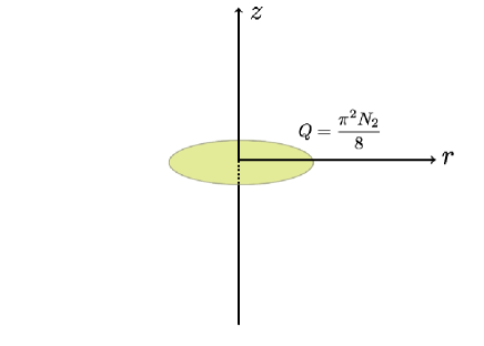
Figure 2: The electrostatic system for the D2-brane solution.

The supergravity solution given by the potential (3.2) has two interesting scaling limits in which the solution becomes the D2-brane solution or the NS5-brane solution constructed in [11]. Let us first consider the limit to the D2-brane solution. The D2-brane solution is given by the same form as (3.1). The electrostatic system for this solution consists of a background potential

$$V_{D2}=W_{0}(r^{2}-2z^{2})$$ (3.12)

with $W_{0}$ constant and a finite size disk at $z=0$ with charge $Q=\pi^{2}N_{2}/8$. Here, the system has no infinite surface and the whole region of $z\in(-\infty,\infty)$ is considered as shown in Fig. 2. See [11] for the explicit form of this solution.

The D2-brane limit is given by redefining the coordinate $z\rightarrow d+z$ and focusing on the finite disk in the electrostatic system of (3.2). The limit is given as

$$d\rightarrow\infty,\;\;\;Q:\;{\rm fixed},\;\;\;V_{0}d=W_{0}:\;{\rm fixed}.$$ (3.13)

From (3.9) and (A.8), we can see that this limit corresponds to the large-$\kappa$ limit. After the redefinition $z\rightarrow d+z$, the background part of (3.2) becomes

$$-\frac{2}{3}V_{0}d^{3}-2V_{0}d^{2}z+V_{0}d(r^{2}-2z^{2})+V_{0}\left(zr^{2}-\frac{2}{3}z^{3}\right).$$ (3.14)

One can neglect the first and second terms since they do not affect the supergravity solution which depends only on $\dot{V},\ddot{V},\dot{V}^{\prime}$ and $V^{\prime\prime}$. So up to these terms, (3.14) indeed becomes (3.12) in the limit of (3.13).

By using the relation (3.11), one can rewrite this limit in terms of the parameters in PWMM as

$$N_{5}\rightarrow\infty,\;\;\;N_{2}:\;{\rm fixed},\;\;\;\frac{4\pi g^{2}}{m^{2}N_{5}}\equiv g^{2}_{S^{2}}:\;{\rm fixed}.$$ (3.15)

The limit corresponds to the commutative limit of fuzzy spheres, where PWMM describes $U(N_{2})$ ${\cal N}=8$ SYM on $R\times S^{2}$. The radius of $S^{2}$ is given by $1/m=1/2$. The fixed quantity $g_{S^{2}}$ in (3.15) is the gauge coupling constant in this theory.

3.3 NS5-brane limit

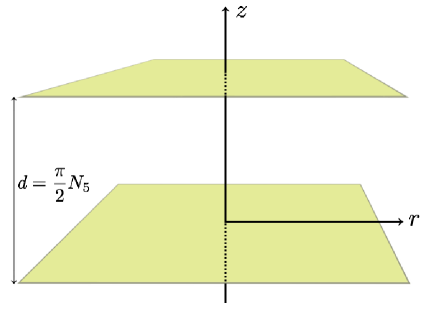
Figure 3: The electrostatic system for the NS5-brane solution.

Let us consider the NS5-brane limit, in which the gravity dual solution written in terms of (3.2) is reduced to the NS5-brane solution constructed in [11]. The NS5-brane solution is given by the form of (3.1), where the electrostatic system now consists of two infinite conducting plates separated by distance $d$ as shown in Fig. 3. The electrostatic potential is given by

$$V_{NS5}(r,z)=\frac{1}{g_{0}}\sin\left(\frac{\pi z}{d}\right)I_{0}\left(\frac{\pi r}{d}\right),$$ (3.16)

where $g_{0}$ is a constant and $I_{n}$ is the modified Bessel function of the first kind. For the explicit form of the geometry, see [11, 14].

The NS5-brane limit is given as a double scaling limit where both $R$ and $V_{0}$ are sent to infinity in an appropriate way. Let us review the derivation of the precise form of the scaling limit [14]. We first make the Fourier expansion of (3.2) in $r<R$ region as,

$$V_{PWMM}(r,z)=V_{0}R^{3}\Delta(\kappa)\frac{z}{d}+\sum_{n=1}^{\infty}c_{n}\sin\left(\frac{n\pi z}{d}\right)I_{0}\left(\frac{n\pi r}{d}\right),$$ (3.17)

where $\kappa\equiv d/R$ and $\Delta(\kappa)$ is defined as

$$\Delta(\kappa)=\beta(\kappa)-\frac{2}{3}\kappa^{3}.$$ (3.18)

The restricted form of the expansion (3.17) follows from the conditions that $V_{PWMM}$ is regular at $r=0$, constant ($V_{0}R^{3}\Delta(\kappa)$) at $z=d$ and zero at $z=0$. Since the first term in (3.17) does not contribute to the geometry, the NS5-brane limit is a limit where

$$c_{1}\rightarrow\frac{1}{g_{0}},\;\;\;\;c_{n}\rightarrow 0\;\;(n>1).$$ (3.19)

One can determine the coefficients $c_{n}$’s by the inverse Fourier transformation at $r=R$ as

$$c_{n}=\left(I_{0}\left(\frac{n\pi}{\kappa}\right)\right)^{-1}2V_{0}R^{3}p_{n}(\kappa),$$ (3.20)

where

$$p_{n}(\kappa)=\int_{0}^{1}dy\left(\phi_{\kappa}(1,\kappa y)-\Delta(\kappa)y-\kappa y+\frac{2}{3}\kappa^{3}y^{3}\right)\sin(n\pi y).$$ (3.21)

When $\kappa=d/R$ is small, $p_{n}(\kappa)$ behaves as

$$p_{n}(\kappa)\sim b_{n}\kappa^{2},$$ (3.22)

where $b_{n}$ are constants. Since $I_{n}(z)\sim e^{z}/\sqrt{2\pi z}$ for $z\gg 1$, we find for small $\kappa$ that

$$c_{n}\sim 2b_{n}\sqrt{2\pi^{2}n}e^{-\frac{n\pi R}{d}}V_{0}(Rd)^{\frac{3}{2}}.$$ (3.23)

Then, the NS5-brane limit is given by

$$R\rightarrow\infty,\hskip 14.22636ptd:\;\text{fixed},\hskip 14.22636ptV_{0}\rightarrow\frac{1}{g_{0}}\frac{1}{2b_{1}\sqrt{2\pi^{2}}}(Rd)^{-\frac{3}{2}}e^{\frac{\pi R}{d}},$$ (3.24)

which realizes (3.19). Note that $\kappa=d/R$ goes to zero in this limit. The value of $b_{1}$ was computed numerically and found to be $b_{1}=0.040$ [14].

Using the relations (3.11), one can rewrite the limit (3.24) in the language of PWMM as

$$N_{2}\rightarrow\infty,\;\;\;\lambda\rightarrow\infty,\;\;\;\frac{1}{N_{2}}\lambda^{\frac{5}{8}}e^{\frac{a}{N_{5}}\lambda^{\frac{1}{4}}}\equiv\tilde{g}_{s}:\;{\rm fixed},\;\;\;N_{5}:\;{\rm fixed},$$ (3.25)

where $a=2\pi^{\frac{1}{2}}/h^{\frac{1}{4}}$ and $\lambda$ is the dimensionless ’t Hooft coupling in PWMM,

$$\lambda=g^{2}N_{2}\left(\frac{2}{m}\right)^{3}.$$ (3.26)

The dual theory of the NS5-brane solution is considered as a six-dimensional non-gravitational string theory called the little string theory (LST). The parameter $\tilde{g}_{s}$ is considered to be the string coupling constant of LST. The limit (3.25) predicts that the dynamics of PWMM near the NS5-brane limit is controlled by $\lambda^{1/4}$. We will confirm this in the next section by analyzing the gauge theory side.

4 Emergent bubbling geometry

In this section, we investigate the matrix integral (2.11) in the parameter region where the dual supergravity description is valid. In order for the supergravity approximation to be valid, the brane charges, $N_{2}$ and $N_{5}$, should be very large and $N_{2}$ should be much larger than $\lambda$ and $N_{5}$ to suppresses the bulk string coupling. In addition, it turns out that the condition $\lambda\gg N_{5}$ is needed to suppress the $\alpha^{\prime}$ corrections. We first show that the matrix integral (2.11) is equivalent to a one-dimensional interacting Fermi gas model. We then study the semi-classical limit of this model, which corresponds to the supergravity regime, by applying the Thomas-Fermi approximation. Under this approximation, the system is described in terms of the mean-field density of the Fermi particles. We find that the mean-field density can be identified with the charge density $f_{\kappa}$ in the gravity side. We also solve the Fermi gas model in the D2-brane and NS5-brane limits and reproduce the radii of the geometries.

4.1 Fermi gas model

Here we show that the matrix integral (2.11) can be mapped to a one-dimensional interacting Fermi gas system with $N_{2}$ particles. We follow the method proposed in [37].

When $N_{5}$ is infinity, the measure factors in (2.11) converge to $\tanh^{2}\frac{\pi(q_{i}-q_{j})}{2}$ up to an over all constant. The $1/N_{5}$ corrections are given as

$$\prod_{J=0}^{N_{5}-1}\frac{[(2J+2)^{2}+(q_{i}-q_{j})^{2}][(2J)^{2}+(q_{i}-q_{j})^{2}]}{[(2J+1)^{2}+(q_{i}-q_{j})^{2}]^{2}}$$

$$\quad=\tanh^{2}\frac{\pi(q_{i}-q_{j})}{2}\exp\left\{\frac{2N_{5}}{(2N_{5})^{2}+(q_{i}-q_{j})^{2}}-\frac{2N_{5}[(2N_{5})^{2}-3(q_{i}-q_{j})^{2}]}{6[(2N_{5})^{2}+(q_{i}-q_{j})^{2}]^{3}}+\cdots\right\},$$ (4.1)

where we have neglected the overall constant. By using the Cauchy identity, we rewrite the hyperbolic tangent part as

$$\prod_{i\neq j}^{N_{2}}\tanh\frac{\pi(q_{i}-q_{j})}{2}=\sum_{\sigma\in S_{N_{2}}}(-)^{\epsilon(\sigma)}\prod_{i=1}^{N_{2}}\frac{1}{\cosh\frac{\pi(q_{i}-q_{\sigma(i)})}{2}},$$ (4.2)

where $\epsilon(\sigma)$ stands for the sign of the permutation $\sigma$.

We introduce the operators, $\hat{p}$ and $\hat{q}$, that obey the canonical Heisenberg algebra $[\hat{p},\hat{q}]=-i$. Let ${\cal H}$ be the usual representation space of this algebra which is an infinite dimensional Hilbert space spanned by the eigenstates of $\hat{q}$. We denote the eigenstates by $|q\rangle$, which satisfy $\hat{q}|q\rangle=q|q\rangle$. Then, we have

$$\frac{1}{\cosh\frac{\pi(q_{i}-q_{j})}{2}}=\frac{1}{\pi}\int dp\,\frac{1}{\cosh p}e^{ip(q_{i}-q_{j})}=\left\langle q_{i}\left|\frac{2}{\cosh\hat{p}}\right|q_{j}\right\rangle.$$ (4.3)

We also introduce the Hilbert space for $N_{2}$ Fermions. It is a subspace of ${\cal H}^{\otimes N_{2}}$ and spanned by the antisymmetric states,

$$\left|q_{1},\cdots,q_{N_{2}}\right\}:=\frac{1}{N_{2}!}\sum_{\sigma\in S_{N_{2}}}(-)^{\epsilon(\sigma)}\left|q_{\sigma(1)}\right\rangle\otimes\left|q_{\sigma(2)}\right\rangle\otimes\cdots\otimes\left|q_{\sigma(N_{2})}\right\rangle.$$ (4.4)

We denote by $\hat{p}_{i}$ and $\hat{q}_{i}$ the canonical pair on the $i$-th Hilbert space. They obey the commutation relations, $[\hat{p}_{i},\hat{q}_{j}]=-i\delta_{ij}$. With these notations, we can rewrite the matrix integral (2.11) as the partition function of a Fermi gas system,

$$Z =\mathrm{Tr}\hat{\rho}$$ (4.5)

where the trace is taken over the states (4.4) as

$$\mathrm{Tr}\hat{\rho}=\int\prod_{i}dq_{i}\left\{q_{1},\cdots,q_{N_{2}}\left|\hat{\rho}\right|q_{1},\cdots,q_{N_{2}}\right\},$$ (4.6)

and the density matrix is given by

$$\hat{\rho}=\prod_{i=1}^{N_{2}}e^{-U(\hat{q}_{i})/2}\prod_{i\neq j}^{N_{2}}e^{-\frac{1}{4}W(\hat{q}_{i}-\hat{q}_{j})}\prod_{i=1}^{N_{2}}e^{-T(\hat{p}_{i})}\prod_{i=1}^{N_{2}}e^{-U(\hat{q}_{i})/2}\prod_{i\neq j}^{N_{2}}e^{-\frac{1}{4}W(\hat{q}_{i}-\hat{q}_{j})}.$$ (4.7)

The functions $T(x)$, $U(x)$ and $W(x)$ are defined as follows.

$$T(x):=\log\cosh x,$$

$$U(x):=\frac{2N_{5}}{g^{2}}x^{2},$$

$$W(x):=-\frac{2N_{5}}{(2N_{5})^{2}+x^{2}}.$$ (4.8)

Here, we have kept only the first term of the exponent in (4.1) because we are interested in the large-$N_{5}$ limit. Even if $N_{5}$ is large, the first term should be kept since it can become comparable to the Gaussian potential in some parameter regions. The model defined by (4.5) is an interacting one-dimensional Fermi gas system of $N_{2}$ fermions, where the interaction is given by $W(q_{i}-q_{j})$.

The semi-classical limit of this model is described by the many-body Hamiltonian,

$$\hat{H}=\sum_{i}T(\hat{p}_{i})+\sum_{i}U(\hat{q}_{i})+\frac{1}{2}\sum_{i\neq j}W(\hat{q}_{i}-\hat{q}_{j}).$$ (4.9)

When $N_{2}$ is large, we can apply the Thomas-Fermi approximation at zero temperature (see in appendix C) to the system (4.9). In this approximation, the original many-body path integral can be evaluated at a saddle point characterized by the mean-field density $\rho(q)$. $\rho(q)$ is assumed to have a single support $[-q_{m},q_{m}]$ and it is normalized as

$$\int_{-q_{m}}^{q_{m}}dq\,\rho(q)=N_{2}.$$ (4.10)

$\rho(q)$ is determined by (C.9) which follows from the Thomas-Fermi equation at zero temperature. In our case, the equation (C.9) is given by

$$\mu=\pi\rho(q)+\frac{2N_{5}}{g^{2}}q^{2}-\int_{-q_{m}}^{q_{m}}dq^{\prime}\,\frac{2N_{5}}{(2N_{5})^{2}+(q-q^{\prime})^{2}}\rho(q^{\prime}),$$ (4.11)

where $\mu$ is the chemical potential. Here, we have made an approximation that $T(p)=\log\cosh p\sim|p|$. This is valid when $N_{2}$ is large.

The equation (4.11) can also be obtained from the usual saddle-point analysis for matrix integrals, where $\rho(q)$ is interpreted as the eigenvalue density. By noting that $\log\tanh^{2}\frac{\pi q_{m}x}{2}\rightarrow-\pi\delta(x)$ as $q_{m}\rightarrow\infty$, one can see that (4.11) is just a saddle-point equation for the eigenvalue density and $\mu$ plays the role of the Lagrange multiplier which imposes the normalization (4.10). So the semi-classical equation (4.11) is expected to be valid when $q_{m}\gg 1$ in the large-$N_{2}$ limit. We will see in section 4.3 that the quantum corrections in the Fermi gas model are indeed negligible when $q_{m}\gg 1$. We will also see that the condition $q_{m}\gg 1$ is written as $\lambda\gg N_{5}$ in terms of the original parameters in PWMM. This is a strong coupling region of PWMM and corresponds to the region in the gravity side where the $\alpha^{\prime}$ corrections are negligible.

4.2 Mapping to the gravity side

The integral equation (4.11) for the mean-field density $\rho(q)$ in the semi-classical limit is the same type as the equation (3.5) for the charge density $f_{\kappa}(x)$ in the gravity dual. So we propose the following identification.

$$\rho(q)=\frac{\mu}{\pi}f_{\kappa}(q/q_{m}),\;\;\;\frac{N_{5}}{q_{m}}=\kappa.$$ (4.12)

Under this identification, (4.11) is completely equivalent to (3.5). In the following, we make consistency checks of the relation (4.12).

Based on the relation (4.12), we first translate the parameters in PWMM to those in the gravity side as follows. First, since $\kappa$ is related to the radius of the disk as $\kappa=d/R=\pi N_{5}/2R$, we have

$$q_{m}=\frac{2}{\pi}R.$$ (4.13)

From the integral equation, we also have

$$\frac{2N_{5}q_{m}^{2}}{\mu g^{2}}=\frac{f^{(0)}_{\kappa}(1)}{f^{(2)}_{\kappa}(1)}.$$ (4.14)

Then, by comparing (3.9) and (4.10), we obtain

$$\frac{N_{2}}{\mu q_{m}}=\frac{q(\kappa)}{\beta(\kappa)}.$$ (4.15)

Finally, from (4.14) and (4.15), we obtain

$$\frac{\lambda}{q_{m}^{4}} =q(\kappa),$$ (4.16)

$$\frac{\mu\lambda}{N_{2}q_{m}^{3}} =\beta(\kappa),$$ (4.17)

where $\lambda=g^{2}N_{2}$ is the ’t Hooft coupling of PWMM. From equations (4.12) and (4.16), we find that $\kappa$ depends only on the combination of $\lambda/N_{5}^{4}$ and $q_{m}$ depends only on $\lambda$ and $N_{5}$.

It should be noted that the relation (4.13) is consistent with the fact that $h$ in (3.11) is a constant and independent of $N_{2}$, $N_{5}$ and $\lambda$. In fact, from (3.9) and (3.11) with (4.13), one can determine $h$ as $h=2/\pi^{2}$. Thus the constant $a=2\pi^{\frac{1}{2}}/h^{\frac{1}{4}}$ in (3.25) is given by

$$a=2^{\frac{3}{4}}\pi.$$ (4.18)

In the following, we consider the D2-brane limit (3.15) and the NS5-brane limit (3.25), which correspond to the large-$\kappa$ limit and the small-$\kappa$ limit, respectively. When $\kappa$ is large, the term with the integral kernel in (4.11) is negligible and the system becomes just a set of $N_{2}$ free fermions. On the other hand, when $\kappa$ is small, the effective interactions between the fermions become very strong. In these two limits, (4.11) is solvable and we can find solutions for $\rho(x)$ and $q_{m}$. Then from the relations (3.10) and (4.13), we can compute the radii of $S^{5}$’s as the range of the mean-field density as,

$$R_{S^{5}}^{2}=2\pi q_{m}.$$ (4.19)

We will show that the radii obtained from the Fermi gas model through (4.19) agree with known results obtained from the gravity solutions [11].

D2-brane limit (large-$\kappa$ limit)

On the gravity side, D2-brane limit corresponds to the limit of large-$\kappa$. In this limit, we can find solutions for $\beta(\kappa)$, $q(\kappa)$ and $f_{\kappa}(q)$ by solving the integral equation (3.5). The solutions are given by (A.8) in appendix A.

From the relations, (4.12), (4.16) and (4.17), one can then obtain solutions for $\rho(q)$, $q_{m}$ and $\mu$ in the Fermi gas model as

$$\rho(q) =N_{2}\left(\frac{9N_{5}}{8\pi\lambda}\right)^{\frac{1}{3}}\left[1-\left(\frac{q}{q_{m}}\right)^{2}\right],\;\;\;q_{m}=\left(\frac{3\pi\lambda}{8N_{5}}\right)^{\frac{1}{3}},\;\;\;\mu=N_{2}\left(\frac{9\pi^{2}N_{5}}{8\lambda}\right)^{\frac{1}{3}}.$$ (4.20)

The parameter $\kappa$ on the gravity side is given by

$$\kappa =\frac{2}{(3\pi)^{\frac{1}{3}}}\left(\frac{N_{5}^{4}}{\lambda}\right)^{\frac{1}{3}}.$$ (4.21)

So the D2-brane limit (3.15) in PWMM is indeed mapped to the limit of $\kappa\rightarrow\infty$ through the identification (4.12).

In the D2-brane limit, PWMM is reduced to $U(N_{2})$ $\mathcal{N}=8$ SYM on $R\times S^{2}$. The gravity dual of $\mathcal{N}=8$ SYM on $R\times S^{2}$ around the trivial vacuum is constructed in [11]. It is shown that the radius of $S^{5}$ at the edge of the disk is related to the ’t Hooft coupling in the SYM as

$$R_{S^{5}}^{2}=\pi\left(3g^{2}_{S^{2}}N_{2}\right)^{\frac{1}{3}}.$$ (4.22)

Here, the coupling constant $g_{S^{2}}$ in SYM is related to that in PWMM as shown in (3.15). On the other hand, we can compute the $S^{5}$ radius in the D2-brane limit from our solutions (4.20). By substituting the solution (4.20) for $q_{m}$ to the relation (4.19), we can reproduce (4.22). This shows the consistency of our identification (4.12).

By using the solution (4.20) of the Fermi gas model, one can compute correlators in this limit. For example, the vev of the loop operator is given by

$$\frac{1}{N_{2}N_{5}}\left\langle\mathrm{Tr}e^{lM}\right\rangle_{MM}=\frac{1}{N_{2}}\int_{-q_{m}}^{q_{m}}dq\rho(q)e^{lq}=\frac{3}{l^{3}q_{m}^{3}}\left\{(lq_{m})\cosh(lq_{m})-\sinh(lq_{m})\right\}.$$ (4.23)

The free energy $F$ defined in (C.12) is given by

$$F=-\frac{9}{10}\left(\frac{\pi^{2}N_{5}}{3\lambda}\right)^{\frac{1}{3}}N_{2}^{2}.$$ (4.24)

Note that the free energy is a generating function of $\mathrm{Tr}M^{2}$. Correlation functions of this operator can be computed as derivatives of the free energy. For example,

$$\frac{1}{N_{2}N_{5}}\langle\mathrm{Tr}M^{2}\rangle_{MM}=-\frac{1}{2N_{2}^{2}N_{5}}\frac{\partial}{\partial(1/\lambda)}F=\frac{(9\pi^{2})^{\frac{1}{3}}}{20}\left(\frac{\lambda}{N_{5}}\right)^{\frac{2}{3}}.$$ (4.25)

Of course, this agrees with the quadratic term in $l$ in (4.23).

One can also solve the path integral (2.11) in this limit by applying the usual saddle-point technique. See appendix D.

NS5-brane limit (small-$\kappa$ limit)

On the gravity side, the NS5-brane limit is a limit of small $\kappa$. When $\kappa$ is small, $\beta(\kappa)$, $q(\kappa)$ and $f_{\kappa}(q)$ are solved by (A.6) in appendix A.

In this limit, from (4.12), (4.16) and (4.17), we obtain solutions $\rho(q)$, $q_{m}$ and $\mu$ for the Fermi gas model as

$$\rho(q)=\frac{8^{\frac{3}{4}}N_{2}}{3\pi\lambda^{1/4}}\left[1-\left(\frac{q}{q_{m}}\right)^{2}\right]^{\frac{3}{2}},\;\;q_{m}=(8\lambda)^{\frac{1}{4}},\;\;\mu=\frac{8^{\frac{1}{2}}N_{2}N_{5}}{\lambda^{\frac{1}{2}}}.$$ (4.26)

The parameter $\kappa$ on the gravity side is given by

$$\kappa =\frac{N_{5}}{(8\lambda)^{\frac{1}{4}}}.$$ (4.27)

So the NS5-brane limit (3.25) in PWMM, which implies $\lambda\sim N_{5}^{4}(\log N_{2})^{4}\gg N_{5}^{4}$, is consistently mapped to the small-$\kappa$ limit. Furthermore, we can see from (4.26) that the typical scale of the mean-field density is given by $\lambda^{1/4}$. So the dynamics in this regime is governed by $\lambda^{1/4}$ as mentioned in the last section.

The gravity dual of PWMM in the small-$\kappa$ limit is studied in [11]. The radius of $S^{5}$ at the edge of the disk is given as

$$R_{S^{5}}^{2}=2\pi(8\lambda)^{\frac{1}{4}}.$$ (4.28)

Again we can reproduce this result from the solution (4.26) in the Fermi gas model, by using (4.19). This gives another supporting evidence for our identification (4.12).

The vev of the loop operator in this limit is given by

$$\frac{1}{N_{2}N_{5}}\left\langle\mathrm{Tr}e^{lM}\right\rangle_{MM}=\frac{2\sqrt{2}}{l^{2}}\lambda^{-\frac{1}{2}}I_{2}\left[l(8\lambda)^{\frac{1}{4}}\right].$$ (4.29)

The free energy $F$ is given by

$$F=-\frac{4\sqrt{2}N_{5}}{3\lambda^{\frac{1}{2}}}N_{2}^{2}.$$ (4.30)

The vev of $\mathrm{Tr}M^{2}$ can also be computed as

$$\frac{1}{N_{2}N_{5}}\langle\mathrm{Tr}M^{2}\rangle_{MM}=-\frac{1}{2N_{2}^{2}N_{5}}\frac{\partial}{\partial(1/\lambda)}F=\frac{\sqrt{2}}{3}\lambda^{\frac{1}{2}}.$$ (4.31)

4.3 Range of the semi-classical approximation

In this subsection, we consider when the semi-classical approximation used in section 4.1 is valid. We first expand the partition function (4.5) around the semi-classical limit by using the Wigner transformation. The Wigner transform of an operator $\hat{A}$ on ${\cal H}$ is defined by

$$A_{W}(q,p)=\int dq^{\prime}\,\left\langle q-\frac{q^{\prime}}{2}\left|\hat{A}\right|q+\frac{q^{\prime}}{2}\right\rangle e^{ipq^{\prime}}.$$ (4.32)

It is easy to see that the product of two operators $\hat{A}$ and $\hat{B}$ is translated to the $\star$-product of their Wigner transforms:

$$(\hat{A}\hat{B})_{W}=A_{W}\star B_{W},$$ (4.33)

where the $\star$-product is defined by

$$(f\star g)(p,q)=f(p,q)\exp\left[\frac{i}{2}(\overleftarrow{\partial}_{q}\overrightarrow{\partial}_{p}-\overleftarrow{\partial}_{p}\overrightarrow{\partial}_{q})\right]g(p,q).$$ (4.34)

The trace is written as the integral over the phase space:

$$\mathrm{Tr}\hat{A}=\int\frac{dqdp}{2\pi}A_{W}(q,p).$$ (4.35)

Hence, the partition function (4.5) becomes

$$Z=\mathrm{Tr}\hat{\rho}=\int\prod_{i}\frac{dq_{i}dp_{i}}{2\pi}\rho_{W}.$$ (4.36)

We define

$$\mathcal{U}_{i}:=U(q_{i})+\frac{1}{2}\sum_{j\neq i}^{N_{2}}W(q_{i}-q_{j}).$$ (4.37)

Then using the Baker-Campbell-Hausdorff formula, we obtain the expansion around the semi-classical limit as

$$\rho_{W} =e^{-\sum_{i}\mathcal{U}_{i}/2}\star e^{-\sum_{i}T(p_{i})}\star e^{-\sum_{i}\mathcal{U}_{i}/2}$$

$$=\exp\left\{\textstyle-\sum_{i}\left(T(p_{i})+\mathcal{U}_{i}\right)-\frac{1}{24}\left[\sum_{i}\left(2T(p_{i})+\mathcal{U}_{i}\right),\left[\sum_{j}T(p_{j}),\sum_{k}\mathcal{U}_{k}\right]_{\star}\right]_{\star}+\cdots\right\},$$ (4.38)

where the star commutator is defined by $[f,g]_{\star}=f\star g-g\star f$. Note that the density matrix is Hermitian, so that only terms with the even number of commutators appear in the right-hand side.

Then let us consider when we can neglect the correction terms in (4.38) that have the star commutators. We always assume the large-$N_{2}$ limit where the saddle-point configurations dominate. Let us denote the orders (magnitudes) of $q_{i}$, $p_{i}$, $T(q_{i})$ and $\mathcal{U}_{i}$ at the saddle point by $q$, $p$, $T$ and $\mathcal{U}$, respectively. (From the symmetry, the order should be the same for any $i=1,\dots,N_{2}$.) These orders are related as follows. First, at the saddle point, the kinetic energy and the potential energy should be in equilibrium. So we have $T={\mathcal{U}}$. Secondly, in the large-$N_{2}$ limit, $T(p_{i})$ is approximated by $|p_{i}|$, so that we also have $T=p$. Thirdly, since the Fermi momentum is related to $\rho(q)$ by (C.8) and $\rho(q)$ satisfies the normalization (4.10), it follows that $p=N_{2}/q$. Thus we have

$$T={\mathcal{U}}=p=N_{2}/q.$$ (4.39)

Note that $pq=N_{2}$ is large. The semi-classical part (the first term of the exponent in (4.38)) looks like the order of $N_{2}(T+{\mathcal{U}})\sim N_{2}^{2}/q$. However, this is not true in general. Near the NS5-brane limit, there is a cancellation between $\sum_{i}T(p_{i})$ and $\frac{1}{2}\sum_{i\neq j}W(q_{i}-q_{j})$, so the order is given by $\sum_{i}U(q_{i})\sim N_{2}^{2}N_{5}q^{2}/\lambda$. The order of the commutator term, $\left[\sum_{i}T(p_{i}),\left[\sum_{j}T(p_{j}),\sum_{k}\mathcal{U}_{k}\right]_{\star}\right]_{\star}$, is given by $N_{2}T^{2}\mathcal{U}/(pq)^{2}\sim N_{2}^{2}/q^{3}$. Hence, if

$$q^{5}\gg\frac{\lambda}{N_{5}},$$ (4.40)

the commutator term is negligible. Then let us consider the higher order terms. Note that, since $T$ is approximated by $p$ in our limit, the commutator terms with more than one $\mathcal{U}$ in (4.38) vanish. Then, the general higher order terms take the form of $[T,[T,[\cdots,[T,\mathcal{U}]\cdots]]]$. The order of such a term with $2m$ $T$’s and one $\mathcal{U}$ is estimated as $N_{2}\mathcal{U}/q^{2m}\sim N_{2}^{2}/q^{2m+1}$. So these terms are suppressed compared to the term with a single commutator, if

$$q\gg 1.$$ (4.41)

So we find that when (4.40) and (4.41) are satisfied, the semi-classical approximation is valid.

However, it turns out that one of the two conditions, (4.40) and (4.41), is redundant, namely, they are equivalent to each other for the saddle-point configurations. In fact, we can see that both of these conditions are equivalent to the following single condition which is written in terms of the original parameters in PWMM.

$$\lambda\gg N_{5}.$$ (4.42)

For example, one can show that (4.42) follows from (4.40) as follows. In the D2-brane limit, $q_{m}$ is given in (4.20). So (4.40) implies (4.42). Similarly, the NS5-brane limit corresponds to $1\gg\kappa=N_{5}/q_{m}\sim N_{5}/\lambda^{1/4}$ which implies (4.42). (Note that we always assume $N_{5}\gg 1$.) When $\kappa$ is in the intermediate region, (4.42) should also be satisfied, because $q(\kappa)$ is a smooth positive function of $\kappa$. In fact, if $\kappa=\frac{N_{5}}{q_{m}}\sim 1$, we have $\lambda\sim N^{4}_{5}$ from (4.16). This implies (4.42). In the same way, one can derive (4.40) from (4.41), and (4.41) from (4.42). Therefore, the three conditions, (4.40), (4.41) and (4.42), are all equivalent.

From (4.19), we see that the condition (4.41) corresponds to the case of large radius of the $S^{5}$. So the semi-classical regime of the Fermi gas system corresponds consistently to the region in the gravity side in which we can neglect the $\alpha^{\prime}$ corrections.

5 Summary and discussion

The gravity dual of the plane wave matrix model (PWMM) is given by bubbling geometries in type IIA superstring theory. These geometries are associated with the problem of an axially symmetric electrostatic system with some conducting disks and an appropriate background potential, which is defined on a certain two-dimensional subspace of the ten-dimensional space-time. The solution is written only in terms of a single function, which corresponds to the electrostatic potential in the axially symmetric system. Once one finds the potential by solving the Laplace equation of the system, one can construct the corresponding solution in the ten-dimensional supergravity. In this paper, we studied an emergent phenomena for this geometry by investigating a quarter BPS sector of the plane wave matrix model that is associated with the field $\phi$ defined in (2.5). Since $\phi$ is a complex field and has two real degrees of freedom, the emergent geometry described in this sector is expected to be a two-dimensional surface ${\cal M}_{\phi}$. We identified ${\cal M}_{\phi}$ with the two-dimensional surface on the gravity side on which the electrostatic problem is defined.

We considered PWMM around the vacua (2.3) with (2.4). We applied the localization method to the sector of $\phi$ and obtained a matrix integral. We investigated the case with $\Lambda=1$ and mapped the matrix integral to a one-dimensional interacting Fermi gas system. And then we applied the Thomas-Fermi approximation which is valid in the semi-classical limit. We found that the mean-field density of the Fermi particles satisfies the same integral equation as the disk charge density in the electrostatic problem on the gravity side. Then, we proposed the identification (4.12) of these two objects. Since the whole geometry can be reconstructed from the charge density, this relation gives a realization of the emergent geometry in PWMM.

We made some consistency checks of our identification and obtained positive results. We consider two scaling limits, the D2-brane limit and the NS5-brane limit. In these limits, the gravity dual of PWMM is reduced to the solutions associated with the corresponding branes. We found that the D2-brane and the NS5-brane limits correspond to the free and the strongly coupled limits in the Fermi gas system, respectively. By solving the Fermi gas system in these limits, we found the value of $a$ in (3.25), which was not fixed solely by the argument in [14]. We reproduced the radius of $S^{5}$’s in the D2-brane and the NS5-brane geometries in terms of the solutions of the Fermi gas model. These results strongly support our identification between the mean-field density and the charge density. In particular, our result in the NS5-brane limit reproduces the known behavior of the fivebrane radius proportional to $\lambda^{1/4}$[15] and it gives a strong evidence for the description of fivebranes in PWMM proposed in [15].

There remain some problems that are not considered in this paper. First, our analysis in the NS5-brane limit is valid only in the planar limit. It corresponds to the leading order of the string coupling constant, $\tilde{g}_{s}$ defined in (3.25), in the little string theory. However, the existence of the NS5-brane limit (3.25) in PWMM should also be verified for higher orders in $\tilde{g}_{s}$. For example, it will be possible to compute the index in PWMM to see if it agrees in the fivebrane limit with the index of a six-dimensional (2,0) superconformal field theory [38, 39], which is supposed to be the low energy theory of LST. Also another useful relation to check the existence of the NS5-brane limit was proposed in [14]. Suppose that the NS5-brane limit exists in PWMM and an operator ${\cal O}$ in PWMM has a good scaling law under the NS5-brane limit, then the coefficients $f_{n}$ of the ’t Hooft expansion $\langle{\cal O}\rangle=\sum_{n}f_{n}/N_{2}^{2n}$ satisfy

$$\frac{f_{n+1}}{f_{n}}=c\lambda^{5/4}e^{2a\frac{\lambda^{1/4}}{N_{5}}},$$ (5.1)

where $c$ is a constant. This relation is obtained by equating the ’t Hooft expansion and the expansion with respect to $\tilde{g}_{s}$. By adding the $1/N_{2}$ corrections to the analysis of the Fermi gas model in the NS5-brane limit, we may be able to answer this problem.

Secondly, though we studied the vacua (2.4) with $\Lambda=1$ in this paper, the sector of $\phi$ can be mapped to a Fermi gas system also in the case of $\Lambda\neq 1$. In this case the Fermi particles have a labeling, $s=1,\cdots,\Lambda$, and the form of the interaction depends on $s$. The remaining problem is whether we can see the emergent geometry in such a general situation.

Thirdly, the bubbling geometries were also constructed for other $SU(2|4)$ symmetric field theories such as ${\cal N}=8$ SYM on $R\times S^{2}$ and ${\cal N}=4$ SYM on $R\times S^{3}/Z_{k}$. The double scaling limits to the NS5-brane solutions were also proposed for these theories [40]. On the gauge theory side, the localization was also applied to these theories [18]. So we can study these cases in the same manner as PWMM.

We hope to report on these issues in the near future.

Appendix A Definition of $f^{(n)}_{\kappa}(x)$

$f^{(n)}_{\kappa}(x)$ is defined as a function satisfying the following Fredholm integral equation of the second kind [14],

$$f^{(n)}_{\kappa}(x)-\int_{-1}^{1}dyK_{\kappa}(x,y)f^{(n)}_{\kappa}(y)=x^{n},$$ (A.1)

with kernel

$$K_{\kappa}(x,y)=\frac{1}{\pi}\frac{2\kappa}{4\kappa^{2}+(x-y)^{2}}.$$ (A.2)

For integer $n$, $f^{(n)}_{\kappa}(-x)=(-1)^{n}f^{(n)}_{\kappa}(x)$. $f^{(0)}_{\kappa}(x)$ and $f^{(2)}_{\kappa}(x)$ are relevant for our problem. In the large-$\kappa$ or the small-$\kappa$ limit, one can solve this integral equation.

Small-$\kappa$ limit

For $\kappa\ll 1$, the solution of (A.1) can be approximated to

$$\frac{1}{2\kappa}\int_{-1}^{1}dyk(x,y)x^{n}$$ (A.3)

with

$$k(x,y)=\frac{1}{2\pi}\log\left\{\frac{1-xy+\sqrt{(1-x^{2})(1-y^{2})}}{1-xy-\sqrt{(1-x^{2})(1-y^{2})}}\right\}.$$ (A.4)

For $n=0$ and $n=2$, (A.3) is evaluated as

$$f^{(0)}_{\kappa}(x) \simeq\frac{1}{2\kappa}(1-x^{2})^{\frac{1}{2}},$$

$$f^{(2)}_{\kappa}(x) \simeq\frac{1}{2\kappa}\left\{\frac{1}{2}(1-x^{2})^{\frac{1}{2}}-\frac{1}{3}(1-x^{2})^{\frac{3}{2}}\right\}.$$ (A.5)

In this case, $\beta(\kappa)$, $q(\kappa)$ and $f_{\kappa}(x)$ introduced in section 3 are given by

$$\beta(\kappa) \simeq\kappa,$$

$$q(\kappa) \simeq\frac{1}{8},$$

$$f_{\kappa}(x) \simeq\frac{1}{3\kappa}(1-x^{2})^{\frac{3}{2}}.$$ (A.6)

Large-$\kappa$ limit

For $\kappa\gg 1$, one can neglect the second term of the left-hand side of (A.1). So, for $n=0$ and $n=2$, the leading behavior is

$$f^{(0)}_{\kappa}(x) \simeq 1,$$

$$f^{(2)}_{\kappa}(x) \simeq x^{2}.$$ (A.7)

Hence, $\beta(\kappa)$, $q(\kappa)$ and $f_{\kappa}(x)$ are approximated to

$$\beta(\kappa) \simeq 2\kappa,$$

$$q(\kappa) \simeq\frac{8}{3\pi}\kappa,$$

$$f_{\kappa}(x) \simeq 1-x^{2}.$$ (A.8)

Appendix B Off-shell supersymmetries in PWMM

In this appendix, we review an off-shell supersymmetries which leave $\phi$ defined in (2.5) invariant [18]. We use the convention in [18]. In particular, we work in the Lorentzian signature by making a Wick rotation $iX_{10}\rightarrow X_{0}$, so that the bosonic symmetry of PWMM is now $R\times SO(3)\times SO(5,1)$. See appendix A in [18] for the definitions of the gamma matrices $\Gamma$ and $\tilde{\Gamma}$ used below.

The supersymmetry transformation in PWMM is given by

$$\delta_{s}X_{M} =-i\Psi\Gamma_{M}\epsilon,$$

$$\delta_{s}\Psi =\left(\frac{1}{2}F_{MN}\Gamma^{MN}-\frac{1}{2}X_{m}\tilde{\Gamma}^{m}\Gamma^{a}\nabla_{a}\right)\epsilon,$$ (B.1)

where the index $a$ runs from $1$ to $4$, $\nabla_{1}=\frac{\partial}{\partial\tau}$ and $\nabla_{2,3,4}$ are defined as

$$\nabla_{a^{\prime}}\epsilon=\frac{1}{4}\varepsilon_{a^{\prime}b^{\prime}c^{\prime}}\Gamma^{b^{\prime}c^{\prime}}\epsilon,$$ (B.2)

The primed indices run from $2$ to $4$. $\epsilon$ is a real conformal Killing spinor with 16 components satisfying

$$\nabla_{a}\epsilon=\tilde{\Gamma}_{a}\tilde{\epsilon},$$ (B.3)

where $\tilde{\epsilon}$ is another real spinor satisfying

$$\Gamma^{a}\nabla_{a}\tilde{\epsilon} =-\frac{1}{2}\epsilon.$$ (B.4)

Here $\epsilon$ is Grassmann even, so that $\delta_{s}$ is Grassmann odd. One can easily solve these equations with the ansatz $\tilde{\epsilon}=\pm\frac{1}{2}\Gamma^{19}\epsilon$, for which (B.3) and (B.4) become

$$\nabla_{a}\epsilon=\pm\frac{1}{2}\Gamma^{a}\Gamma^{19}\epsilon.$$ (B.5)

Then, the solution is given by

$$\epsilon_{+}=\begin{pmatrix}e^{\frac{\tau}{2}}\ \eta_{1}\\ 0\\ e^{-\frac{\tau}{2}}\ \eta_{3}\\ 0\\ \end{pmatrix}\quad\text{and}\quad\epsilon_{-}=\begin{pmatrix}0\\ e^{-\frac{\tau}{2}}\ \eta_{2}\\ 0\\ e^{\frac{\tau}{2}}\ \eta_{4}\end{pmatrix},$$ (B.6)

for the upper and the lower sign in (B.5), respectively. $\eta_{1,2,3,4}$ are four-component constant spinors. One can see that when the SUSY parameter is given by $\epsilon_{+}$ with $\eta_{3}=-J_{4}\eta_{1}$, $\phi$ is invariant, $\delta_{s}\phi=0$. See [18] for the notation of $J_{4}$.

By introducing seven auxiliary fields $K_{i}(i=1,2,\cdots,7)$ with the quadratic action,

$$\frac{1}{g^{2}}\int d\tau\frac{1}{2}{\rm Tr}K_{i}K_{i},$$ (B.7)

one can make the SUSY off-shell [41],

$$\delta_{s}X_{M}=-i\Psi\Gamma_{M}\epsilon,$$

$$\delta_{s}\Psi=\frac{1}{2}F_{MN}\Gamma^{MN}\epsilon-X_{m}\tilde{\Gamma}^{m}\Gamma^{19}\epsilon+K^{i}\nu_{i},$$

$$\delta_{s}K_{i}=i\nu_{i}\Gamma^{M}D_{M}\Psi.$$ (B.8)

Here, ${\nu_{i}}$ are spinors which can be determined by the closure of the SUSY algebra. In particular, when $\epsilon$ is given by $\epsilon_{+}$ in (B.6) with $\eta_{3}=-J_{4}\eta_{1}$, these spinors are explicitly given by

$$\nu_{i}=\sqrt{2}e^{\frac{\tau}{2}\Gamma^{09}}e^{-\frac{\pi}{4}\Gamma^{49}}\Gamma^{i8}\begin{pmatrix}\eta_{1}\\ 0\\ 0\\ 0\end{pmatrix}.\;\;\;\;\;(i=1,2,\cdots,7)$$ (B.9)

Since $\{\Gamma^{M^{\prime}}\epsilon,\;\nu^{i}|M^{\prime}=1,\cdots,9,\;i=1,\cdots,7\}$ forms the orthogonal basis of 16 component spinors, $\Psi$ can be decomposed as

$$\Psi=\Psi_{M^{\prime}}\Gamma^{M^{\prime}}\epsilon+\Upsilon_{i}\nu^{i}.$$ (B.10)

We also define

$$H_{i} :=(\epsilon\epsilon)K_{i}+2\nu_{i}\tilde{\epsilon}X_{0}+s_{i},$$ (B.11)

$$s_{i} :=\nu_{i}\left(\frac{1}{2}\sum_{P,Q=1}^{9}F_{PQ}\Gamma^{PQ}\epsilon-2\sum_{m=5}^{9}X_{m}\Gamma^{m}\tilde{\epsilon}\right).$$ (B.12)

For the SUSY with $\epsilon_{+}$ with $\eta_{3}=0$, by introducing the collective notation,

$$X :=\begin{pmatrix}X_{M^{\prime}}\\ (\epsilon\epsilon)\Upsilon_{i}\end{pmatrix},\;\;X^{\prime}:=\begin{pmatrix}-i(\epsilon\epsilon)\Psi_{M^{\prime}}\\ H_{i}\end{pmatrix},$$

the transformation rules can be written in a compact form as

$$\delta_{s}X=X^{\prime},\;\;\;\delta_{s}X^{\prime}=-i(\delta_{\phi}+\delta_{U(1)})X,\;\;\;\delta_{s}\phi=0.$$ (B.13)

Here, $\delta_{U(1)}$ is a variation under a $U(1)$ subgroup of the $SO(3)\times SO(5,1)$ and $\delta_{\phi}$ is a gauge transformation with the parameter $\phi$. One can see that $\delta_{s}\Psi_{1}$ is proportional to $\delta_{\phi}X_{1}=D_{1}\phi$ as mentioned above (2.10).

Appendix C Thomas-Fermi approximation

In this appendix, we review the Thomas-Fermi approximation, which is the semi-classical limit of the Hartree approximation. We consider a one-dimensional many-body system at finite temperature $1/\beta$ that has a one-body Hamiltonian of the form $h(q,p)=T(p)+U(q)$ and a two-body interaction potential $W(q,q^{\prime})$. The Hartree approximation is just the saddle-point evaluation of the path integral of this system and becomes exact when the particle number $N$ goes to infinity. In this approximation, the saddle point is characterized by the mean-field density $\rho(x)$ that satisfies the normalization

$$\int dq\rho(q)=N.$$ (C.1)

$\rho(x)$ is determined by the following Hartree equation.

$$\rho(q)=\left\langle q\left|\frac{1}{e^{\beta(H(\hat{p},\hat{q})-\mu)}+1}\right|q\right\rangle,$$ (C.2)

where $\mu$ is the chemical potential and $H(p,q)$ is the effective one-body Hamiltonian defined by

$$H(p,q)=T(p)+U(q)+\int dq^{\prime}W(q,q^{\prime})\rho(q^{\prime}).$$ (C.3)

If one obtains $\rho(x)$ by solving the equation (C.2), then from (C.1) one can also compute the first derivative of the grand potential as

$$\frac{\partial J}{\partial\mu}=\int dq\rho(q).$$ (C.4)

The free energy is given by

$$F=\log Z=J(\mu(N))-\mu(N)N.$$ (C.5)

In the semi-classical limit, the Hartree equation (C.2) reduces to

$$\rho(q)=\int\frac{dp}{2\pi\hbar}\frac{1}{e^{\beta(H(p,q)-\mu)}+1}.$$ (C.6)

This equation is called the Thomas-Fermi equation at finite temperature. When the temperature goes to zero, the equation (C.6) is further simplified to

$$\rho(q)=\int\frac{dp}{2\pi\hbar}\theta(\mu-H(p,q)).$$ (C.7)

Let us assume that the Fermi surface $\{(p,q)|\mu=H(p,q)\}$ is simply connected and symmetric under $p\rightarrow-p$. Then (C.7) implies that $\rho(q)$ is given by

$$\rho(q)=\frac{p_{F}(q)}{\pi\hbar},$$ (C.8)

where $p_{F}(q)$ is the Fermi momentum. From the definition of $p_{F}(q)$, we obtain the following integral equation that determines $\rho(q)$.

$$\mu=T(\pi\hbar\rho(q))+U(q)+\int dq^{\prime}W(q,q^{\prime})\rho(q^{\prime}).$$ (C.9)

This equation can be regarded as an extremization condition for the Thomas-Fermi functional,

$$E_{\mathrm{TF}}[\rho]=\int dq\>t_{\mathrm{TF}}(q)+\int dq\rho(q)U(q)+\frac{1}{2}\int dqdq^{\prime}\rho(q)W(q,q^{\prime})\rho(q^{\prime})-\mu\left(\int dq\rho(q)-N\right)$$ (C.10)

where $t_{\mathrm{TF}}(q)$ is the kinetic energy functional

$$t_{\mathrm{TF}}(q)=\int\frac{dp}{2\pi\hbar}T(p)\theta(\mu-H(p,q)),$$ (C.11)

and $\mu$ is the Lagrange multiplier associated with the constraint (C.1), which can be identified with the chemical potential at the saddle point. The free energy is given by (C.10) with $\rho$ satisfying (C.9);

$$F=-\mathrm{min}_{\rho}\>E_{\mathrm{TF}}[\rho].$$ (C.12)

Appendix D Saddle-point method for the D2-brane limit

In this appendix, we solve our matrix integral for the D2-brane limit in the planar limit by applying the usual saddle-point method [42]. We assume the one-cut solution. The matrix integral in this limit is given by

$$Z=\int\prod_{i}dq_{i}\prod_{i<j}\tanh^{2}\left(\frac{\pi(q_{i}-q_{j})}{2}\right)e^{-\frac{2\pi}{g_{S^{2}}^{2}}\sum_{i}q_{i}^{2}}.$$ (D.1)

By changing the integral variables to $z_{i}:=\exp(\pi q_{i}+g^{2}_{S^{2}}\pi/4)$, the path integral is reduced to

$$Z=\int\prod_{i}dz_{i}\prod_{i>j}\left(\frac{z_{i}-z_{j}}{z_{i}+z_{j}}\right)^{2}e^{-\frac{2}{g_{S^{2}}^{2}\pi}\sum_{i}(\log z_{i})^{2}}.$$ (D.2)

The saddle-point equation is given by

$$\frac{2}{g^{2}_{S^{2}}\pi}\frac{\log z_{i}}{z_{i}}-\sum_{j(\neq i)}\left(\frac{1}{z_{i}-z_{j}}-\frac{1}{z_{i}+z_{j}}\right)=0.$$ (D.3)

Note that this equation is symmetric under the inversion, $z_{i}\rightarrow 1/z_{i}$. Let $[a,b]$ be the support of the eigenvalue distribution of $z_{i}$. From the inversion symmetry, it follows that $b=1/a$. We define the resolvent as

$$W(z)=4g^{2}_{S^{2}}\pi\sum_{i}\left(\frac{1}{z-z_{i}}-\frac{1}{z+z_{i}}\right).$$ (D.4)

This function has two branch cuts at $[a,b]$ and $[-b,-a]$. The eigenvalue distribution,

$$\rho(z)=\frac{1}{N_{2}}\sum_{i}\delta(z-z_{i}),$$ (D.5)

can be expressed as the discontinuity of $W(z)$ as usual,

$$W(z+i0)-W(z-i0)=-8\pi^{2}ig^{2}_{S^{2}}N_{2}\rho(z).$$ (D.6)

We introduce a new variable $y=z^{2}$. The resolvent is also a holomorphic function of $y$. So let us denote $W(z)=P(y)$, where $P(y)$ is holomorphic in $y$. $P(y)$ has a single cut at $[a^{2},b^{2}]$ on the $y$-plane. Using (D.3), one can easily get

$$P(y+i0)+P(y-i0)=\frac{8\log y}{\sqrt{y}},$$ (D.7)

where $y\in[a^{2},b^{2}]$. By defining a new function,

$$\hat{P}(y)=\frac{P(y)}{\sqrt{(y-a^{2})(y-b^{2})}},$$ (D.8)

one can convert (D.7) to the discontinuity equation,

$$\hat{P}(y+i0)-\hat{P}(y-i0)=\frac{1}{\sqrt{(y-a^{2})(y-b^{2})}}\frac{8\log y}{\sqrt{y}}.$$ (D.9)

This equation determines $\hat{P}$ up to the regular part. Since $\hat{P}(y)\sim y^{-2}$ when $y\rightarrow\infty$, the regular part should be vanishing. Thus, we obtain

$$\hat{P}(y)=\int_{a^{2}}^{b^{2}}\frac{dp}{2\pi}\frac{8\log p}{(y-p)\sqrt{p}}\frac{1}{\sqrt{(p-a^{2})(b^{2}-p)}},$$ (D.10)

and then the resolvent is given by

$$W(z)=32\int_{a}^{b}\frac{dq}{2\pi}\frac{\log q}{z^{2}-q^{2}}\sqrt{\frac{(z^{2}-b^{2})(z^{2}-a^{2})}{(b^{2}-q^{2})(q^{2}-a^{2})}}.$$ (D.11)

From (D.6), the eigenvalue distribution is given by

$$\rho(x)=\frac{4}{\pi^{3}g^{2}_{S^{2}}N_{2}}P\int_{a}^{b}dq\frac{\log q}{q^{2}-x^{2}}\sqrt{\frac{(b^{2}-x^{2})(x^{2}-a^{2})}{(b^{2}-q^{2})(q^{2}-a^{2})}},$$ (D.12)

where $x\in[a,b]$ and $P\int$ means the principal value. Note that it satisfies

$$x\rho(x)=\frac{1}{x}\rho(1/x).$$ (D.13)

When the ’t Hooft coupling $g^{2}_{S^{2}}N_{2}$ is large, the integral in (D.12) can be performed. This limit will turn out to correspond to the large-$b$ limit. By changing the variables in (D.12) as

$$\log b=-\log a=\alpha,\;\;\;\log x=v\alpha,\;\;\;\log q=u\alpha,$$ (D.14)

one can obtain

$$x\rho(x)+\frac{1}{x}\rho(1/x)=\frac{4\alpha^{2}}{\pi^{3}g^{2}_{S^{2}}N_{2}}P\int_{-1}^{1}du\;u\;{\rm sign}(u-v)+{\cal O}(\alpha^{1}).$$ (D.15)

Then, the integral can be easily performed. By using (D.13), one obtains

$$\rho(x)=\frac{2}{\pi^{3}g^{2}_{S^{2}}N_{2}}\frac{(\log b)^{2}-(\log x)^{2}}{x},$$ (D.16)

in the leading order of $\alpha$. Since $\int_{a}^{b}\rho(x)dx=1$ by definition, $b$ is determined as

$$b=1/a=\exp\left[\pi\left(\frac{3g^{2}_{S^{2}}N_{2}}{8}\right)^{\frac{1}{3}}\right].$$ (D.17)

Thus, $b$ is indeed large when the ’t Hooft coupling is large.

Using (D.16), one can easily compute the free energy of the matrix integral. The result is given by

$$\log Z=\frac{9\pi}{10}\frac{N^{2}_{2}}{(3g_{S^{2}}^{2}N_{2})^{1/3}}.$$ (D.18)

References

- [1] J. M. Maldacena, Adv. Theor. Math. Phys. 2 (1998) 231 [arXiv:hep-th/9711200].
- [2] S. S. Gubser, I. R. Klebanov and A. M. Polyakov, Phys. Lett. B 428 (1998) 105 [arXiv:hep-th/9802109].
- [3] E. Witten, Adv. Theor. Math. Phys. 2 (1998) 253 [arXiv:hep-th/9802150].
- [4] D. Berenstein, JHEP 0601, 125 (2006) [hep-th/0507203].
- [5] D. E. Berenstein, M. Hanada and S. A. Hartnoll, JHEP 0902, 010 (2009) [arXiv:0805.4658 [hep-th]].
- [6] H. Steinacker, Class. Quant. Grav. 27, 133001 (2010) [arXiv:1003.4134 [hep-th]].
- [7] S. -W. Kim, J. Nishimura and A. Tsuchiya, Phys. Rev. Lett. 108, 011601 (2012) [arXiv:1108.1540 [hep-th]].
- [8] H. S. Yang, arXiv:1312.0580 [hep-th].
- [9] D. Berenstein, J. M. Maldacena and H. Nastase, JHEP 0204 (2002) 013 [arXiv:hep-th/0202021].
- [10] T. Banks, W. Fischler, S. H. Shenker and L. Susskind, Phys. Rev. D 55, 5112 (1997) [hep-th/9610043].
- [11] H. Lin and J. M. Maldacena, Phys. Rev. D 74, 084014 (2006) [hep-th/0509235].
- [12] H. Lin, O. Lunin and J. M. Maldacena, JHEP 0410, 025 (2004) [hep-th/0409174].
- [13] H. Lin, JHEP 0412, 001 (2004) [hep-th/0407250].
- [14] H. Ling, A. R. Mohazab, H. -H. Shieh, G. van Anders and M. Van Raamsdonk, JHEP 0610, 018 (2006) [hep-th/0606014].
- [15] J. Maldacena, M. M. Sheikh-Jabbari and M. Van Raamsdonk, JHEP 0301 (2003) 038 [arXiv:hep-th/0211139].
- [16] V. Pestun, Commun. Math. Phys. 313, 71 (2012) [arXiv:0712.2824 [hep-th]].
- [17] N. A. Nekrasov, Adv. Theor. Math. Phys. 7, 831 (2004) [hep-th/0206161].
- [18] Y. Asano, G. Ishiki, T. Okada and S. Shimasaki, JHEP 1302, 148 (2013) [arXiv:1211.0364 [hep-th]].
- [19] D. Berenstein, JHEP 0407, 018 (2004) [hep-th/0403110].
- [20] Y. Takayama and A. Tsuchiya, JHEP 0510, 004 (2005) [hep-th/0507070].
- [21] M. Bianchi and S. Kovacs, Phys. Lett. B 468, 102 (1999) [hep-th/9910016].
- [22] B. Eden, P. S. Howe, C. Schubert, E. Sokatchev and P. C. West, Phys. Lett. B 472, 323 (2000) [hep-th/9910150].
- [23] O. Aharony, M. Berkooz, S. Kachru, N. Seiberg and E. Silverstein, Adv. Theor. Math. Phys. 1, 148 (1998) [hep-th/9707079].
- [24] E. Witten, JHEP 9707, 003 (1997) [hep-th/9707093].
- [25] N. Arkani-Hamed, A. G. Cohen, D. B. Kaplan, A. Karch and L. Motl, JHEP 0301, 083 (2003) [hep-th/0110146].
- [26] M. R. Douglas, JHEP 1102, 011 (2011) [arXiv:1012.2880 [hep-th]].
- [27] C. Bachas, J. Hoppe and B. Pioline, JHEP 0107, 041 (2001) [hep-th/0007067].
- [28] J. -T. Yee and P. Yi, JHEP 0302, 040 (2003) [hep-th/0301120].
- [29] H. Lin, Phys. Rev. D 74, 125013 (2006) [hep-th/0609186].
- [30] S. Sugishita and S. Terashima, JHEP 1311, 021 (2013) [arXiv:1308.1973 [hep-th]].
- [31] D. Honda and T. Okuda, arXiv:1308.2217 [hep-th].
- [32] K. Hori and M. Romo, arXiv:1308.2438 [hep-th].
- [33] V. A. Kazakov, I. K. Kostov and N. A. Nekrasov, Nucl. Phys. B 557, 413 (1999) [hep-th/9810035].
- [34] Y. Kitazawa, S. ’y. Mizoguchi and O. Saito, Phys. Rev. D 74, 046003 (2006) [hep-th/0603189].
- [35] G. Ishiki, Y. Takayama and A. Tsuchiya, JHEP 0610, 007 (2006) [hep-th/0605163].
- [36] G. Ishiki, S. Shimasaki, Y. Takayama and A. Tsuchiya, JHEP 0611 (2006) 089 [arXiv:hep-th/0610038].
- [37] M. Marino and P. Putrov, arXiv:1206.6346 [hep-th].
- [38] H. -C. Kim, J. Kim and S. Kim, arXiv:1211.0144 [hep-th].
- [39] H. -C. Kim, S. Kim, S. -S. Kim and K. Lee, arXiv:1307.7660.
- [40] H. Ling, H. -H. Shieh and G. van Anders, JHEP 0702, 031 (2007) [hep-th/0611019].
- [41] N. Berkovits, Phys. Lett. B 318, 104 (1993) [hep-th/9308128].
- [42] T. Suyama, Nucl. Phys. B 856, 497 (2012) [arXiv:1106.3147 [hep-th]].