MRRR-based Eigensolvers for Multi-core Processors and Supercomputers

Abstract

The real symmetric tridiagonal eigenproblem is of outstanding importance in numerical computations; it arises frequently as part of eigensolvers for standard and generalized dense Hermitian eigenproblems that are based on a reduction to tridiagonal form. For its solution, the algorithm of Multiple Relatively Robust Representations (MRRR or MR³ in short) – introduced in the late 1990s – is among the fastest methods. To compute $k$ eigenpairs of tridiagonal $T\in\mathbb{R}^{n\times n}$, MRRR only requires $\mathcal{O}(kn)$ arithmetic operations; in contrast, all the other practical methods require $\mathcal{O}(k^{2}n)$ or $\mathcal{O}(n^{3})$ operations in the worst case. This thesis centers around the performance and accuracy of MRRR.

First, we investigate how MRRR can make efficient use of modern multi-core architectures. We present a parallelization strategy that dynamically divides and schedules the work into tasks. This task-based approach is flexible and produces remarkable workload balancing. In a number of experiments, comparing our multi-threaded eigensolver, mr3smp, with the widely used LAPACK (Linear Algebra PACKage) and Intel’s Math Kernel library (MKL), we show that mr3smp outperforms even the fastest solvers available.

Second, for massively parallel distributed/shared-memory systems, we introduce an eigensolver, PMRRR, that merges the task-based approach with a parallelization based on message-passing. Our design uses non-blocking communications, thus allowing processes to proceed computation while waiting to receive data. Experimentally, we show the importance of such an overlap of computation and communication for load balancing and scalability. Moreover, with a thorough performance study, we demonstrate that the new eigensolvers of the Elemental library, which are based on PMRRR, are faster and more scalable than the widely used eigensolvers of ScaLAPACK.

Third, we present a mixed precision variant of MRRR, which improves the standard algorithm in multiple ways. In fact, compared with the best available methods (Divide & Conquer and the QR algorithm), the standard MRRR exhibits inferior accuracy and robustness. Moreover, when confronted with heavily clustered eigenvalues, its performance and scalability can suffer severely; such scalability problems especially arise on distributed-memory architectures. Our mixed precision approach makes MRRR at least as accurate as Divide & Conquer and the QR algorithm. In particular in context of direct methods for large-scale standard and generalized Hermitian eigenproblems, such an improvement comes with little or no performance penalty: eigensolvers based on our mixed precision MRRR are oftentimes faster than solvers based on Divide & Conquer and, in some circumstances, even faster than solvers based on the standard MRRR. Additionally, the use of mixed precisions considerably enhances robustness and parallel scalability.

Chapter 1 Motivation & Contributions

1.1 Motivation

The algorithm of Multiple Relatively Robust Representations (MRRR or MR³ in short) is a method for computing a set of eigenvalues and eigenvectors (i.e., eigenpairs) of a real symmetric tridiagonal matrix [40, 44, 43, 118, 119]. The algorithm achieves what has been sometimes called the “holy grail of numerical linear algebra” [78]: It is capable of computing $k$ eigenpairs of tridiagonal $T\in\mathbb{R}^{n\times n}$ with $\mathcal{O}(kn)$ arithmetic operations, while all the other existing methods require $\mathcal{O}(k^{2}n)$ or $\mathcal{O}(n^{3})$ operations in the worst case. For this reason, its invention by Dhillon and Parlett [40, 44, 43] in the late 1990s was widely acknowledged as a breakthrough in the field. The method was expected to be (almost always) faster than all existing methods, while being equally accurate. Furthermore, it promised to be embarrassingly parallel and thus ideally suited for parallel computers. In light of these expectations, early after its introduction, it was natural to believe that the MRRR algorithm would make all the other methods obsolete. After roughly 15 years of experience with the algorithm, this has not been the case for a number of reasons.

Speed.

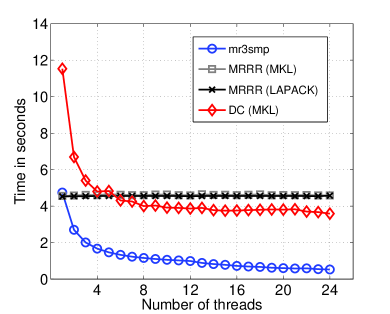
A detailed investigation on the performance and accuracy of LAPACK’s [5] symmetric tridiagonal eigensolvers revealed that, although MRRR performs the fewest floating point operations (flops), due the phenomenon of numerical deflation and its higher flop-rate (flops per second), the Divide & Conquer algorithm (DC) can be faster [37]. Not investigated in [37] is how the performance is influenced by the parallelism of modern architectures. For a matrix of size $4{,}289$ and by increasing the number of computational threads, Fig. 1.1 illustrates that, although MRRR is the fastest sequential method, as the amount of available parallelism increases, DC becomes faster than MRRR.

(a) Execution time.

(b) Breakdown of time by stages.

Figure 1.1: (a) Timings as function of the number of threads used in the computation. Qualitatively, the graph is typical for the applications matrices that we tested. As the available parallelism increases, DC becomes faster than MRRR. (b) Fraction of time spent in the solution of the real symmetric dense eigenproblem for (1) reduction to tridiagonal form, (2) tridiagonal eigenproblem, and (3) backtransformation of the eigenvectors. For details of the experiment, see [122].

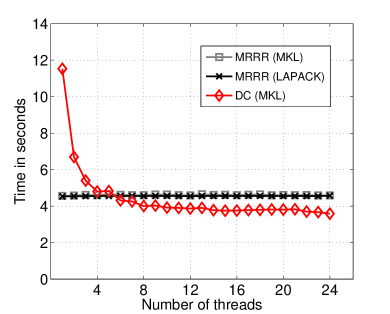
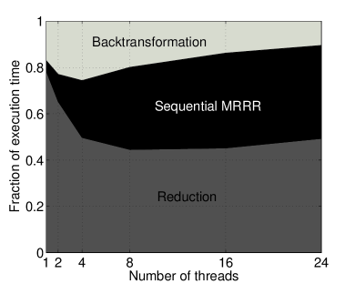
The reason for this behavior is that DC casts most of the work in terms of matrix-matrix multiplication and takes advantage of parallelism by multi-threaded Basic Linear Algebra Subprograms (BLAS) [97, 49, 50]. In contrast, neither LAPACK’s MRRR nor the version included in Intel’s MKL exploit any parallelism offered by multiple cores. Figure 1.1(b) displays that, since MRRR does not scale, it can become a significant portion of the common three stage approach to the dense Hermitian eigenproblem.

Scalability.

Today, parallel computing is everywhere. While for many years the usage of parallel computers was limited to high-end products, the advent of multi-core processors has revolutionized the world of computing: Performance improvements of existing sequential code will not occur by simply waiting for the next generation of processors, but by explicitly exploiting the available parallelism [149]. Since multi-core processors became the standard engines for both commodity computers (desktops and laptops) and supercomputers, the sequential computation model became obsolete and replaced by parallel paradigms [133]. Given the current trends in the development of computer hardware, it is expected that the number of processing units (cores) of uniprocessors and supercomputers increase rapidly in the near future. In light of this development, many algorithms and existing software must be reevaluated and rewritten and it becomes increasingly important how well algorithms can exploit the ever growing parallelism [7, 74].

A number of software packages (like LAPACK and ScaLAPACK) address the need for eigensolvers on both uniprocessor and distributed-memory architectures. However, at the time of beginning this dissertation, the support for multi-core architectures and mixed distributed/shared-memory architectures was limited. Explicit exploitation of shared-memory was largely confined to methods that rely heavily on multi-threaded BLAS. On a uniprocessor, methods that do not make use of suitable BLAS kernels – e.g., MRRR – cannot exploit any parallelism beyond that at the instruction level and, consequently, do not scale.

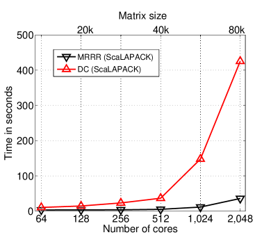
Despite the initial expectations on MRRR, the computation is not embarrassingly parallel. However, as demonstrated by Bientinesi et al. [13] and later Vömel [162], MRRR is well suited for parallel computations. Existing parallel implementations – ParEig [13] and ScaLAPACK [20, 162] – target distributed-memory architectures. On multi-core architectures, those implementations require the availability and initialization of a message-passing library and are penalized by the redundant computations they perform to avoid costly communication. Furthermore, they might not achieve load balancing due to static workload division. Even on distributed-memory systems, neither ScaLAPACK’s MRRR – added to the library in 2011 [162] – nor alternatives like ScaLAPACK’s DC scale perfectly to a large number of processor cores, as illustrated in Fig. 1.2. All these factors motivated research that targets multi-core architectures and hybrid distributed/shared-memory architectures specifically.

(a) 1–2–1 type matrices.

(b) Wilkinson type matrices.

Figure 1.2: Weak scalability (the matrix size is increased according to the number of cores) for the computation of all eigenpairs of two different test matrix types. Each type provides an example in which one of the two solvers performs rather poorly for highly parallel executions. The left and right graphs have different scales. For MRRR the execution time should remain roughly constant. For details of the experiment, see [124].

Accuracy.

The aforementioned study also shows that MRRR is less accurate than DC or the QR algorithm (QR) [37]. Especially for large-scale problems, both residuals and orthogonality of the computed eigenpairs are inferior, cf. [37, Figure 6.1] and [175, Table 5.1]. In our experience, as depicted in Fig. 1.3, the disadvantages are mainly confined to the orthogonality.

(a) Largest residual norm.

(b) Orthogonality.

Figure 1.3: Accuracy of LAPACK’s MRRR and DC for a set of test matrices from the Stetester [104] test suite, ranging in size from $1{,}000$ to about $8{,}000$. The results for QR are similar to the ones of DC.

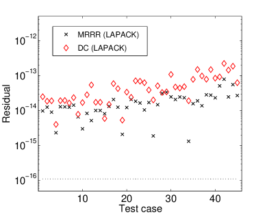
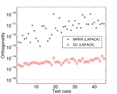
Through increased robustness, Willems and Lang [174, 178, 176] were able to improve the orthogonality. Nonetheless, their analysis [175] shows that the accuracy of any MRRR implementation is inferior to those of DC and QR. For instance, “one must be prepared for orthogonality levels of about $\mathcal{O}(1000n\varepsilon)$, [where $\varepsilon$ denotes the unit roundoff,] because they can occur even if all of the requirements [of the algorithm] are fulfilled with very benign parameters” [175].

Robustness.

The QR algorithm has been analyzed for more than half a century, which led to extremely robust implementations. MRRR – with a number of novel features – was only introduced in the 1990s and, almost naturally, its use on challenging problems brought forth non-satisfactory results and even failure [45]. The causes of failure were soon identified and mostly eliminated [45, 174]. In particular, the research of Vömel, Willems and Lang improved the reliability of the method [45, 174, 178, 176]. Even though MRRR usually gives satisfactory results, there is a problem not quite apparent to a user: The proofs of correctness in [43, 175] hinge on finding so called relatively robust representations (RRRs) of the input matrix with shifted spectrum. A representation is accepted as an RRR if it passes a simple test, which is frequently the case. However, sometimes no representation is found that passes the test and instead a promising candidate is selected, which might or might not fulfill the requirements. In such a situation, accuracy is not guaranteed. Willems and Lang reduce – but not eliminate – this problem by expanding the forms a representation can take [178, 176], changing the shifting strategy, and using a more sophisticated test for relative robustness [164, 175]. Nevertheless, for some input matrices, the accuracy of MRRR cannot be guaranteed.

1.2 Contributions

In this dissertation, we make four main contributions:

1. We introduce a strategy, MR³-SMP, specifically tailored for current multi-core and future many-core processors. Our design makes efficient use of the on-chip parallelism and the low communication overhead thanks to the shared-memory and caches. Parallelism is achieved by dynamically dividing the computation into tasks that are executed by multiple threads. We show that the task-based approach scales well on multi-core processors and small shared-memory systems made out of them; in most cases, it scales better than state-of-the-art eigensolvers for uniprocessors and distributed-memory systems. Good speedups are observed even in the case of relatively small matrices. For the example in Fig. 1.1, the results of our solver mr3smp are shown in Fig. 1.4. With the exploitation of parallelism, independent of the number of threads used for the computation, MRRR remains faster than DC. The good scalability of the tridiagonal eigensolver is reflected in the execution time of the dense Hermitian problem. While previously the fraction of the tridiagonal stage was up to 40% of the total execution time [Fig. 1.1(b)], the fraction spent in the tridiagonal stage is reduced to less than 7% [Fig. 1.4(b)].

   

   (a) Execution time.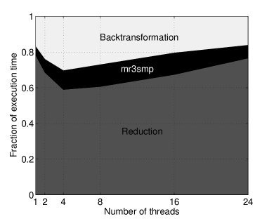

   

   (b) Breakdown of time by stages.

   Figure 1.4: (a) Timings as function of the number of threads used in the computation. Qualitatively, the graph is typical for the applications matrices that we tested. (b) Fraction of time spent in the solution of the corresponding real symmetric dense eigenproblem for (1) reduction to tridiagonal form, (2) tridiagonal eigenproblem, and (3) backtransformation of the eigenvectors. For details of the experiment, see [122].

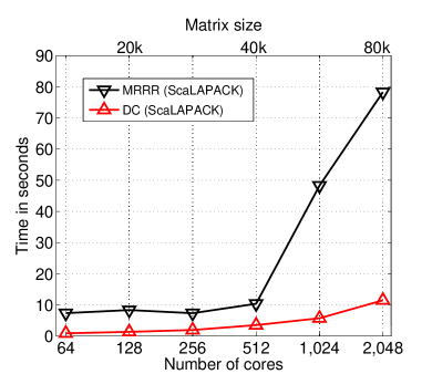
2. For massively parallel distributed/shared-memory architectures, we develop a variant of MRRR that merges the task-based approach with the parallelization strategy proposed by Bientinesi et al. [13]. Our new solver, PMRRR, can make use of messages-passing for inter-node communication and shared-memory for intra-node communication. It can also be used in a purely message-passing or shared-memory mode, allowing the user to decide which programming model to employ. Our design uses non-blocking communications in conjunction with a task-based approach, which enables processes to proceed the computation while waiting to receive data. Such an overlap of computation and communication is crucial for load balancing and scalability. For the example in Fig. 1.2, the results are shown in Fig. 1.5.

   

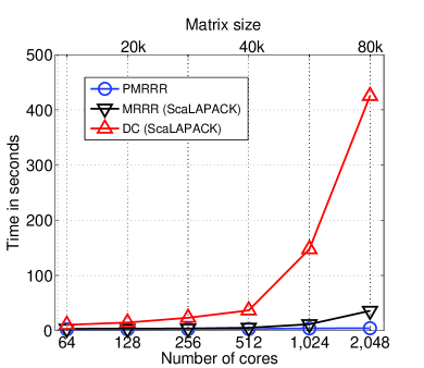
   (a) 1–2–1 type matrices.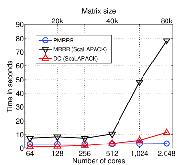

   

   (b) Wilkinson type matrices.

   Figure 1.5: Weak scalability (the matrix size is increased according to the number of cores) for the computation of all eigenpairs of two different test matrix types. The left and right graphs have different scales. For MRRR the execution time should remain roughly constant. For details of the experiment, see [124].

   For instance, in the experiment with a Wilkinson type matrix on 1024 cores, ScaLAPACK’s MRRR spends about 30 out of 50 seconds in exposed communication. As Fig. 1.5(b) demonstrates, even for matrices that strongly favor DC, due to its superior scalability, eventually our solver becomes faster than ScaLAPACK’s DC.

3. PMRRR is integrated into Elemental, a development framework and library for distributed-memory dense linear algebra, which can now be used to solve large-scale dense eigenproblems. We perform a thorough performance study of Elemental’s new eigensolvers on two high-end computing platforms. A comparison with the widely used ScaLAPACK eigensolvers reveals that each ScaLAPACK routine present performance penalties that are avoided by calling a different sequence of subroutines and choosing suitable settings. We show how to built – within the ScaLAPACK framework – an eigensolver faster than the existing ones. By comparing Elemental’s eigensolvers with the standard ScaLAPACK solvers as well as the ones build according to our guidelines, we show that Elemental is fast and highly scalable.

4. We present a variant of MRRR based on mixed precisions, which addresses the existing weaknesses of the algorithm: ($i$) inferior accuracy compared with DC or QR; ($ii$) the danger of not finding suitable representations; and ($iii$) for distributed-memory architectures, load balancing problems and communication overhead for matrices with large clustering of the eigenvalues. Our approach adopts a new perspective: Given input/output arguments in a binary_ x floating point format, we use a higher precision binary_y arithmetic to obtain the desired accuracy. An analysis shows that we gain enormous freedom to choose important parameters of the algorithm. In particular, we are able to select these parameters to reduce the operation count, increase robustness, and improve parallelism; at the same time, we meet more stringent accuracy goals [Fig. 1.6].

   

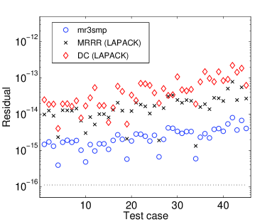
   (a) Largest residual norm.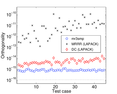

   

   (b) Orthogonality.

   Figure 1.6: For real symmetric tridiagonal matrices with dimension from $1{,}000$ to about $8{,}000$, accuracy of our mixed precision solver compared with LAPACK’s DC and MRRR.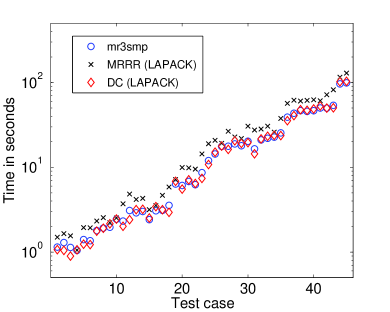

   

   (a) Execution time: multi-threaded.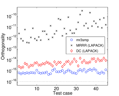

   

   (b) Orthogonality.

   Figure 1.7: For real symmetric dense matrices with dimension from $1{,}000$ to about $8{,}000$, time and accuracy of our mixed precision solver compared with LAPACK’s DC and MRRR.

   This work is mainly motivated by the performance study of Elemental’s eigensolvers. In the context of dense eigenproblems, the tridiagonal stage is often completely negligible in terms of execution time: to compute $k$ eigenpairs of a tridiagonal matrix, it only requires $\mathcal{O}(kn)$ operations; the reduction to tridiagonal form requires $\mathcal{O}(n^{3})$ operations and is the performance bottleneck. In terms of accuracy, the tridiagonal stage is responsible for most of the loss of orthogonality. The natural question is whether it is possible to improve the accuracy to the level of the best methods without sacrificing too much performance. We show that this is indeed possible. In fact, our mixed precision solver is more accurate than the ones based on DC or QR [Fig. 1.7(b)], and remains as fast as the classical MRRR [Fig. 1.7(a)]. Finally, an important feature of the mixed precision approach is a considerably increased robustness and parallel scalability.

1.3 Outline of the thesis

In Chapter 2, we give background material concerning eigenproblems. In particular, we focus on methods for real symmetric tridiagonal eigenproblems and direct methods for standard and generalized Hermitian eigenproblems. We introduce basic terminology, existing algorithms, and available software. We also quantify goals such as accuracy, scalability, and load balance. A reader familiar with the above issues can safely skip all or parts of Chapter 2.

In Chapter 3, we focus on the MRRR algorithm and its most prominent features. We introduce the method to an appropriate level for our purposes. Our goal is neither to provide a rigorous exposition nor all the numerous details of MRRR. Instead, the chapter serves – together with Chapter 2 – as a basis for the later discussion of Chapters 4 and 5. Therefore, we focus on features that are important for parallelization and introduce the factors that influence parallelism, robustness, and accuracy. An expert of MRRR will not find anything new and can safely skip all or parts of Chapter 3.

In Chapter 4, we introduce our work on parallel versions of MRRR targeting modern multi-core and hybrid distributed/shared-memory architectures. Section 4.1 presents the task-based parallelization strategy for multi-core architectures. Section 4.2 presents PMRRR, which merges the task-based parallelization with a parallelization for distributed-memory architectures via message-passing. We further discuss Elemental’s new eigensolvers for dense Hermitian eigenproblems, which make use of PMRRR, and their performance compared with ScaLAPACK.

Finally, in Chapter 5, we introduce our mixed precision approach for MRRR. We demonstrate how it improves accuracy, robustness, and parallelism. Experiments indicate that these benefits come with little or even no extra cost in terms of performance.

Chapter 2 Background & Related Work

In this chapter, we compile background material concerning basic terminology, existing algorithms, and state-of-the-art software. The organization is as follows: Section 2.1 introduces the Hermitian eigenproblem (HEP) and summarizes its basics properties. In Section 2.2, we comment on our notation. In Section 2.3, we give a brief overview of the existing methods with special emphasis on the real symmetric tridiagonal eigenproblem (STEP), which is the main focus of this dissertation. We then return to the more general HEP and introduce existing methods, in particular, direct methods based on a reduction to tridiagonal form. The discussion of the HEP is important for two reasons: first, it demonstrates that the STEP underlies most methods for the HEP, and second, in later chapters, we show results of our solvers in the context of direct methods for the HEP, referring to the material of this chapter repeatedly. For the same reasons, we briefly discuss the generalized Hermitian eigenproblem (GHEP). In Section 2.4, we list popular software that implements the previously specified algorithms. Finally, in Section 2.5, we list a set of objectives for any eigensolver. These objectives are used to compare different implementations throughout later chapters.

Our discussion is far from complete as “the computation of eigenvalues of matrices is one of the problems most intensively studied by numerical analysts, and the amount of understanding incorporated in state-of-the-art software […] is [tremendous]” [154]. As most of the material can be found in textbooks (e.g., [114, 32, 147, 168, 66, 154]), we limit the content of this chapter to important aspects for this dissertation. Hence, a reader familiar with the basics of Hermitian eigenproblems can safely skip the rest this chapter. For the other readers, we recommend to read this chapter as we use the material and notation without reference in later chapters.

2.1 The Hermitian eigenproblem

The Hermitian eigenproblem (HEP) is the following: Given an Hermitian matrix $A\in\mathbb{C}^{n\times n}$ (i.e., $A=A^{*}$, where $A^{*}$ denotes the complex-conjugate-transpose of $A$), find solutions to the equation

$$Ax=\lambda x\,,$$

where $\lambda\in\mathbb{R}$, $x\in\mathbb{C}^{n}$, and $x\neq 0$. Without loss of generality, we assume $\lVert x\rVert=\sqrt{x^{*}x}=1$ subsequently. For such a solution, $\lambda$ is called an eigenvalue (of $A$) and $x$ an associated eigenvector. An eigenvalue together with an associated eigenvector are said to form an eigenpair, $(\lambda,x)$. In matrix form, the computation of $k$ eigenpairs is written

$$AX=X\Lambda\,,$$

where the eigenvalues are entries of the diagonal matrix $\Lambda\in\mathbb{R}^{k\times k}$ and the associated eigenvectors form the columns of $X\in\mathbb{R}^{n\times k}$.

The HEP is “one of the best understood“ and “the most commonly occurring algebraic” [34] eigenproblems; it has a number of distinct features. In particular, we make use of the following well-known result, cf. [79, Theorem 4.1.5].

Theorem 2.1.1 (Spectral Theorem for Hermitian matrices).

Let $A\in\mathbb{C}^{n\times n}$ be given. Then $A$ is Hermitian if and only if there is a unitary matrix $X\in\mathbb{C}^{n\times n}$, $X^{*}=X^{-1}$, and a diagonal matrix $\Lambda\in\mathbb{R}^{n\times n}$ such that $A=X\Lambda X^{*}$. Proof: See [79, 66].

The decomposition $A=X\Lambda X^{*}$ is called an eigendecomposition of $A$ and, by the Spectral Theorem, such a decomposition always exists for an Hermitian matrix. This is equivalent to saying that $n$ distinct eigenpairs exist, i.e., $Ax_{i}=\lambda_{i}x_{i}$ for $1\leq i\leq n$, where all eigenvalues are real and the eigenvectors can be chosen to form an orthonormal basis for $\mathbb{C}^{n}$. Hence, the eigenvalues can be ordered as

$$\lambda_{1}\leq\lambda_{2}\leq\ldots\leq\lambda_{i}\leq\ldots\leq\lambda_{n}\,,$$

where $\lambda_{i}$ is the $i$-th smallest eigenvalue of $A$. In situations where the underlying matrix is not clear, we write $\lambda_{i}[A]$ explicitly. The set of all eigenvalues is called the spectrum of $A$ and denoted by $spec[A]$.

The eigenvectors can be chosen such that for all $i,j\in\{1,2,\ldots,n\}$,

$$x_{i}^{*}x_{j}=\left\{\begin{array}[]{l l}1&\quad\text{if $i=j$}\,,\\ 0&\quad\text{if $i\neq j$}\,.\\ \end{array}\right.$$ (2.1)

For distinct eigenvalues, corresponding eigenvectors are given as (orthonormal) bases of $\mathcal{N}(A-\lambda_{i}I)$ – the null space of $A-\lambda_{i}I$. This means that the eigenvectors are generally not unique. However, when an eigenvalue $\lambda_{i}$ is simple, i.e., distinct from all the other eigenvalues, then $\mbox{dim}\,\mathcal{N}(A-\lambda_{i}I)=1$ and the corresponding eigenvector is unique up to scaling.

Besides individual eigenvectors, subspaces spanned by a set of eigenvectors – called invariant subspaces – are of special importance. For a given index set $\mathcal{I}\subseteq\{1,2,\ldots,n\}$,

$$\mathcal{X}_{\mathcal{I}}=\mbox{span}\{x_{i}:i\in\mathcal{I}\}$$

denotes the invariant subspace associated with $\mathcal{I}$. As with the eigenvalues, we write $\mathcal{X}_{\mathcal{I}}[A]$ for $\mathcal{X}_{\mathcal{I}}$ whenever the underlying matrix is not understood from context.

When computing eigenpairs, it is useful to have transformations that change the problem in a simple prescribed way. Two of these transformations are shifts and similarities. Transforming $A$ to $A-\sigma I$ is called shifting and $\sigma\in\mathbb{R}$ is called a shift. It is easily verified that $(\lambda,x)$ is an eigenpair of $A$ if and only if $(\lambda-\sigma,x)$ is an eigenpair of $A-\sigma I$. Thus, the spectrum is shifted by $\sigma$ and the eigenvectors are invariant. Similarly, given a nonsingular $Q\in\mathbb{C}^{n\times n}$, transforming $A$ to $Q^{-1}AQ$ is called a similarity transformation or a change of basis. In this case, $(\lambda,x)$ is an eigenpair of $A$ if and only if $(\lambda,Q^{-1}x)$ is an eigenpair of $Q^{-1}AQ$. Thus, the spectrum is invariant under similarity transformations, while the eigenvectors change in a simple way. In particular, if $Q$ is unitary, $Q^{*}=Q^{-1}$, the transformation is called a unitary similarity transformation. Using this notion, the Spectral Theorem states that every Hermitian matrix is unitarily similar to a real diagonal matrix.

An important subclass of the HEP is the real symmetric eigenproblem, which means $A$ is restricted to be real-valued, $A\in\mathbb{R}^{n\times n}$. In this case, all complex-valued quantities become real-valued and the discussion of the HEP holds with the words ’Hermitian’ and ’unitary’ respectively replaced by ’symmetric’ and ’orthogonal’. The focus of this dissertation is on the even more specialized case of real symmetric tridiagonal matrices. Before providing an overview of existing methods for the real symmetric tridiagonal eigenproblem, we give a number of comments regarding our notation throughout this document.

2.2 Notation

Generally, matrices are denoted by upper case Roman or Greek letters, while vectors and scalars are denoted with lower case Roman or Greek letters. The underlying field ($\mathbb{R}$ or $\mathbb{C}$) and the dimensions are specified in context. Some letters and symbols are reserved for special quantities:

• $I$ denotes the identity matrix of appropriate size and $e_{j}$ denotes its $j$-th column, with all elements being zero except the $j$-th, which is one.

• $\lambda$ is used for eigenvalue and is always real-valued in this document.

• $A$ of size $n$-by-$n$ denotes a generic Hermitian matrix, possibly real-valued, with eigenvalues $\lambda_{1}\leq\ldots\leq\lambda_{n}$ and corresponding eigenvectors $x_{1},\ldots,x_{n}$. When computing (a subset of) eigenpairs, $\Lambda$ is the diagonal matrix with the eigenvalues as its entries and $X$ contains the corresponding eigenvectors as columns.

• $T$ of size $n$-by-$n$ denotes a generic real symmetric tridiagonal matrix with eigenvalues $\lambda_{1}\leq\ldots\leq\lambda_{n}$ and corresponding eigenvectors $z_{1},\ldots,z_{n}$. When computing (a subset of) eigenpairs, $\Lambda$ is the diagonal matrix with the eigenvalues as its entries and $Z$ contains the corresponding eigenvectors as columns.

• $\varepsilon$ is used for machine precision or unit roundoff, defined as half the distance between one and the next larger floating point number.

• $spdiam[A]$ denotes the spectral diameter of matrix A, i.e., $spdiam[A]=\lambda_{n}-\lambda_{1}$.

• For $x\in\mathbb{R}^{n}$, $\lVert x\rVert=\sqrt{x^{*}x}$ is the Euclidean norm; $\lVert x\rVert_{1}=\sum_{i=1}^{n}|x(i)|$ is the 1-norm.

• For $A\in\mathbb{C}^{n\times n}$, $\lVert A\rVert=\max\{|\lambda_{1}|,|\lambda_{n}|\}$ denotes the spectral norm; $\lVert A\rVert_{1}=\max_{1\leq j\leq n}\sum_{i=1}^{n}|A(i,j)|$ denotes the 1-norm.

• For $t\in\mathbb{R}$, we use the notation $\mathcal{O}(t)$ informally as “of the order of $t$ in magnitude.” The notion is used to hide moderate constants that are of no particular interest.

Despite $\mathbb{R}\subset\mathbb{C}$, we frequently use the term complex-valued matrix or $A\in\mathbb{C}^{n\times n}$ implying that at least one of its elements is not real-valued. We use $A^{*}$ to denote the complex-conjugate-transpose of matrix $A$. (If $A\in\mathbb{R}^{n\times n}$, $A^{*}$ denotes its transpose.) We use the term Hermitian as the generic term; symmetric, however, is used synonymously with real symmetric, that is, no complex symmetric matrices are encountered in this document. Similarly, a tridiagonal matrix is implicitly real symmetric.

Although eigenvectors are not unique, we talk about the eigenvectors and, although we compute approximations to eigenvalues and eigenvectors, we simply refer to computed eigenvalues and computed eigenvectors. Such computed quantities are represented by hatted symbols (e.g., $\hat{\lambda}$ or $\hat{z}$). The set of computed eigenvectors is numerically orthogonal. We frequently, omit the terms ’set’ and ’numerically’ and say that computed eigenvectors are orthogonal.

The topic of this dissertation is the efficient solution of “large-scale” eigenvalue problems. On a single processor, we consider problems as “small” if the entire input and output fits into the processors cache. Similarly, on a distributed-memory system, we consider problems as “small” if the entire problem can effectively be solved on a uniprocessor system. For instance, for today’s hardware, computing the eigendecomposition of $A\in\mathbb{C}^{5000\times 5000}$ (in IEEE double precision) is considered large on a uniprocessor system, but small on a massively parallel supercomputer.

2.3 Existing methods

Methods differ in various aspects: the number of floating point operations (flops) they have to perform (on average, in the worst case), the flop-rate at which the operations are performed, the amount of memory required, the possibility of computing subsets of eigenpairs at reduced cost, the attainable accuracy (on average, in the worst case), the simplicity and robustness of an implementation, and the suitability for parallel computations. In this section, we comment on the main features of different methods for solving Hermitian eigenproblems in various forms.

2.3.1 The real symmetric tridiagonal eigenproblem

A number of excellent algorithms for the real symmetric tridiagonal eigenproblem exist. Among them, bisection [12, 114, 33] and inverse iteration [169, 121, 172, 84, 41, 82], the QR algorithm [61, 90, 114], the Divide & Conquer algorithm [29, 51, 67, 68], and the method of Multiple Relatively Robust Representations (MRRR) [40, 44, 43, 118, 119]. All four methods are implemented in publicly available software (see Section 2.4) and a user is required to make a selection among the algorithms, each of them with its strengths and weaknesses and without a clear winner in all situations. The “best” algorithm might be influenced by a number of factors: the problem (e.g., size, spectrum, subsets), the architecture (e.g., cache sizes, parallelism), external libraries (e.g., BLAS), and the specific implementation of the algorithm. At this point, we collect the main characteristics of each algorithm; an experimental comparison of their implementations is found in later chapters. Further comparisons – general and experimental – of the algorithms can be found in [37, 40, 13, 78, 32, 34].

We motivate our presentation: The comments about QR demonstrate why the method is, when eigenvectors are desired, not competitive for the STEP. The discussion about DC is important as the method is generally fast, scalable, and accurate; we therefore frequently compare our results to it. We introduce inverse iteration as it is closely related to MRRR; in fact, “it is difficult to understand MRRR without appreciating the limitations of standard inverse iteration” [46]. Finally, MRRR is the main focus of this dissertation and it is described more detailed in Chapter 3; at this point, we only mention its most salient features.

We remark that all four methods are numerically stable and, if completed successfully, computed eigenpairs of input matrix $T$ fulfill

$$\lVert T\hat{z}_{i}-\hat{\lambda}_{i}\hat{z}_{i}\rVert=\mathcal{O}(n\varepsilon\lVert T\rVert)\,,$$ (2.2)

and for $i\neq j$

$$|\hat{z}_{i}^{*}\hat{z}_{j}|=\mathcal{O}(n\varepsilon)\,.$$ (2.3)

MRRR’s accuracy and limitations (not for all inputs accuracy is guaranteed) compared with other methods is the topic of Chapter 5.

Bisection and inverse iteration (BI)

Bisection, which is discussed in more detail in Section 3.2.2, may be used to find an approximation to any eigenvalue with $\mathcal{O}(n)$ arithmetic operations [32, 147]; thus, it computes $k$ eigenvalues requiring only $\mathcal{O}(kn)$ flops. Given an initial interval $[\alpha,\beta]$ which contains a sought after eigenvalue, the interval is bisected until sufficiently small. Roughly $-3n\log_{2}\varepsilon$ flops are required to compute an eigenvalue to sufficient accuracy [40]. Convergence is linear and rather slow. Nonetheless, bisection has a number of great features [114, 33, 103]: (1) It can be used to obtain approximations to just a subset of eigenvalues at reduced cost; (2) It can be used to obtain approximations to low accuracy at reduced cost; (3) It can be used to refine approximate eigenvalues to higher accuracy; (4) It can be used to compute eigenvalues to high relative accuracy (whenever the data defines them to such accuracy); (5) all computations are embarrassingly parallel.

After finding approximations to $k$ eigenvalues via bisection, inverse iteration may be used to compute the corresponding eigenvectors. Inverse iteration is one of the oldest methods for computing selected eigenvectors when given approximations to the eigenvalues. According to an interesting article on the history of the method [81], it was introduced by Wielandt as early as 1944. Given an approximate eigenvalue $\hat{\lambda}_{i}$ of input matrix $T$ and a starting vector $\hat{z}_{i}^{(0)}\in\mathbb{R}^{n}$, the procedure consists of repeated solutions of linear systems: for $k\geq 1$,

$$(T-\hat{\lambda}_{i}I)\hat{z}_{i}^{(k)}=s^{(k)}\hat{z}_{i}^{(k-1)}\,,$$

where $s^{(k)}\in\mathbb{R}$ is a positive scaling factor, say for simplicity chosen such that $\lVert\hat{z}_{i}^{(k)}\rVert=1$. Under mild assumptions, the sequence $\hat{z}_{i}^{(k)}$ converges to an eigenvector approximation $\hat{z}_{i}$ with small residual norm, i.e., such that (2.2) is satisfied. In fact, the residual norm $\lVert r\rVert=\lVert T\hat{z}_{i}^{(k)}-\hat{\lambda}_{i}\hat{z}_{i}^{(k)}\rVert=s^{(k)}$ is readily available and is used to signal convergence [82]. A small residual of $\mathcal{O}(n\varepsilon\lVert T\rVert)$ implies that $(\hat{\lambda}_{i},\hat{z}_{i})$ is an eigenpair of a “close matrix”, that is, there exist a perturbation $E$ such that $(\hat{\lambda}_{i},\hat{z}_{i})$ is an eigenpair of $A+E$ and $\lVert E\rVert\leq\lVert r\rVert$ [82]. However, small residuals (backward errors) are not sufficient to guarantee orthogonality among independently computed eigenvectors – i.e., (2.3) might not hold. Whenever $\hat{\lambda}_{i}$ is not well-separated (in an absolute sense) from the rest of the spectrum, even for a simple eigenvalue, the computed eigenvector $\hat{z}_{i}$ might be a poor approximation to the true eigenvector $z_{i}$. Only if almost all eigenvalues are well-separated, inverse iteration is efficient and requires $\mathcal{O}(kn)$ operations to compute the eigenvectors. In such a scenario, the computation of the eigenvectors is also easily performed in parallel. In contrast, if eigenvalues are clustered, orthogonality must be enforced, usually by means of Gram-Schmidt orthogonalization [1]. This process is potentially costly and requires in the worst case $\mathcal{O}(k^{2}n)$ flops; additionally, parallelism might be lost almost entirely. For large-scale problems, the Gram-Schmidt procedure almost always increases the computation time significantly [13].

Together, bisection and inverse iteration, which is often considered a single method, has the advantage of being adaptable; that is, the method may be used to compute a subset of eigenpairs at reduced cost. For this reason, it is still today probably the most commonly used method for computing subsets of eigenpairs. Unfortunately, current software can fail to deliver correct results [41, 32] and, due to the explicit orthogonalization of eigenvectors, its performance suffers severely on matrices with tightly clustered eigenvalues [32]. While BI has been the method of choice for computing a subset of eigenpairs for many years, the authors of [37] suggest that today MRRR “is preferable to BI for subset computations.”

The QR algorithm (QR)

The QR algorithm is arguably the most ubiquitous tool for the solution of (dense) eigenvalue problems. On that account, it was placed in the list of the top ten algorithms of the 20th century [116]. The algorithm was independently discovered in the 1950s by Francis [61] and Kublanovskaja [90] and has been studied extensively since then. While “for the general, nonsymmetric eigenvalue problem, QR is still king” [167], it faces serious competition in the real symmetric tridiagonal case – for instance, Divide & Conquer, which is usually faster and equally accurate [136, 151].

The method generates a sequence of orthogonally similar tridiagonals $T_{k}=Z_{k}^{*}TZ_{k}$ whose off-diagonal entries are driven rapidly to zero. In other words, $T_{k}$ converges to $\Lambda$, containing the eigenvalues, and $Z_{k}$ converges to $Z$, containing the eigenvectors. For each QR step, $T_{k}=Q_{k}^{*}(Z_{k-1}^{*}TZ_{k-1})Q_{k}$, with $k\geq 1$ and $Z_{0}=I$, $Q_{k}$ is a product of $n-1$ Givens rotations [64], which must be accumulated, $Z_{k}=Z_{k-1}Q_{k}$, if the eigenvectors are desired. The process is guaranteed to converge [170, 77, 114, 166] and leads to simple, robust and elegant implementations. Crucial for performance and convergence are the implicit use of shifted matrices $T_{k}-\sigma_{k}I$ and the exploitation of deflation whenever an off-diagonal is close to zero [114].

When only eigenvalues are desired, the rotations need not be accumulated and the computation can be rearranged such that no square-roots, which are usually more expensive than other operations, are needed. This leads to the so called square-root free QR or the PWK algorithm [111, 134, 114]. This algorithm is quite efficient and requires only about $9n^{2}$ operations to compute all eigenvalues [114]. The square-root free variant – with its $\mathcal{O}(n^{2})$ costs – is frequently used when only eigenvalues are computed on a uniprocessor. On the other hand, alternative methods like bisection are more amendable on parallel computing environments [35].

The cost of QR changes dramatically when also the eigenvectors are desired. In this case, the majority of the work is performed in accumulating the Givens rotations. As the accumulation costs about $3n^{2}$ operation per QR step and roughly $2n$ QR steps are necessary for convergence, about $6n^{3}$ arithmetic operations are necessary in total. For large problems, due to the higher cost compared to other methods, QR is usually not competitive for the STEP when eigenvectors are desired. In contrast to the “eigenvalues only” case, if eigenvectors are desired, the computation is parallelized quite effectively [13, 35].

Divide & Conquer (DC)

DC is among the fastest and most accurate methods available [37, 136, 32, 151]. The method is called by the authors of [154] “the most important advance in matrix eigenvalue algorithms since the 1960s.” It was introduced by Cuppen in 1981 [29], but it took more than a decade to find a stable variant of the algorithm [67, 68]. The divide and conquer strategy works by dividing the problem into two smaller subproblems, which are solved recursively and whose solutions are combined to the solution of the original problem. In our case, the tridiagonal is expressed as rank-one modification of a direct sum of tridiagonals $T_{1}=Z_{1}\Lambda_{1}Z_{1}^{*}$ and $T_{2}=Z_{2}\Lambda_{1}Z_{2}^{*}$:

$$\small T=\left(\begin{array}[]{cc}T_{1}&\\ &T_{2}\end{array}\right)+\rho uu^{*}=\left(\begin{array}[]{cc}Z_{1}&\\ &Z_{2}\end{array}\right)\left[\left(\begin{array}[]{cc}\Lambda_{1}&\\ &\Lambda_{2}\end{array}\right)+\rho vv^{*}\right]\left(\begin{array}[]{cc}Z_{1}^{*}&\\ &Z_{2}^{*}\end{array}\right)\,,$$

where $\rho\in\mathbb{R}$ and $u,v\in\mathbb{R}^{n}$ are readily available without further computation. The problem is solved by recursively applying the procedure to $T_{1}$ and $T_{2}$ to find their eigendecompositions and solving the eigenproblem for a rank-one update of a diagonal matrix: $(\Lambda_{1}\oplus\Lambda_{2})+\rho vv^{*}=Z_{D}\Lambda Z_{D}^{*}$. To complete the computation of $T$’s eigendecomposition, $T=Z\Lambda Z^{*}$, the eigenvectors are found by the matrix-matrix product $Z=(Z_{1}\oplus Z_{2})\cdot Z_{D}$.

Both the eigenvalues and the eigenvectors of a rank-one update of a diagonal matrix are computed efficiently with only $\mathcal{O}(n^{2})$ operations, but the process must be done with great care to be numerically stable [98, 67, 68]. The vast majority of the computation is spent in the matrix-matrix product to obtain $Z$ – hence, it is crucial for performance of the algorithm that an optimized matrix-matrix multiplication is available. Neglecting the cost for computing the eigendecomposition of $(\Lambda_{1}\oplus\Lambda_{2})+\rho vv^{*}$, assuming that all the matrices are dense, the subproblems are of size $n/2$, and a standard matrix multiplication is used, the overall process requires roughly $\frac{4}{3}n^{3}$ flops [32, 147, 150]. However, the method frequently does much better than this because of numerical deflation [51, 136, 150]: Whenever entries of $v$ are sufficiently small in magnitude or two entries in $(\Lambda_{1}\oplus\Lambda_{2})$ are almost equal, some columns of $Z_{D}$ can be made essentially columns of the identity matrix. This means, computations in the matrix-matrix product are saved and eigenpairs of the subproblem (padded with zeros) are accepted as eigenpairs of the larger problem. For both performance and numerical stability, the “deflation process is essential for the success of the divide and conquer algorithm” [150]. The amount of deflation depends on the eigenvalue distribution and the structure of the eigenvectors [40].

Depending on the sample of test matrices and the deflation criterion, a different behavior of the algorithm is observed in practice: in [32, 150] it is reported that for random test matrices “it appears that [the algorithm takes] only $\mathcal{O}(n^{2.3})$ flops on average, and as low as $\mathcal{O}(n^{2})$ for some eigenvalue distributions.” More complete tests in [37] lead to the conclusion that “DC is $\mathcal{O}(n^{2.5})$ measured using time and $\mathcal{O}(n^{2.8})$ measured using flop counts” on average, where the run time behavior is specific to the architecture of the experiment and is explained by an increasing flop-rate with the size of matrix-matrix multiplications.

A big advantage of DC lies in the inherent parallelism of the divide and conquer approach and its reliance on the (usually available) highly optimized matrix-matrix kernel for computing the eigenvectors. The main drawback of the method is that it requires the largest amount of memory of all methods (it requires at least additional $n^{2}$ floating point numbers of workspace [37, 136, 150]). Additionally, most implementations cannot be used to compute a subset of eigenpairs at reduced cost. A study in [8] argues that up to 70% of the compute time is spent in the final two matrix-matrix multiplications, unless extreme deflation takes place, cf. also [136]. By only propagating the desired subset of eigenvectors in these steps, the computation time is reduced by up to a factor three; see [8, 136] for details. While these savings for computing subsets are significant in practice, “the adaptation [of Divide & Conquer] to this case is somewhat artificial” [43]. Similarly, if only eigenvalues are desired, DC requires only $\mathcal{O}(n^{2})$ operations, but other methods, like the square-root free QR Iteration, are often preferred.

Therefore, as stated in [136], “if [enough memory] is available, if the full eigendecomposition is desired, and if either highly optimized BLAS are available or highly clustered eigenvalues are possible, we recommend divide and conquer as the algorithm of choice.” Since all these conditions are frequently satisfied, DC is one of the most commonly used method.

For a pedagogical treatment of the main principles behind DC, we refer to [32, 147, 168]. For the sake of completeness, we mention that the Divide & Conquer method does not exist, but a family of methods varying in different parts of the described procedure. Also, the operation count can be lowered to $\mathcal{O}(n^{2})$ for computing all eigenpairs and $\mathcal{O}(n\log_{2}n)$ for computing only eigenvalues – with implicit constants too high to be used in practice today. As these aspects are not important for our discussion, we simply refer to [32, 68] and the references therein.

Multiple Relatively Robust Representations (MRRR)

To compute $n$ eigenpairs, all the practical methods discussed so far charge $\mathcal{O}(n^{3})$ arithmetic operations in the worst case. The MRRR algorithm is the first stable method that does the job using $\mathcal{O}(n^{2})$ flops. Furthermore, the method is adaptable and computes $k$ eigenpairs in $\mathcal{O}(kn)$ time.

The method was introduced by Dhillon and Parlett in the late 1990s [40]. Proofs of its correctness and a number of improvements were added at the beginning of this century [43, 44, 174]; however, the method remains the subject of active research. It is a variant of inverse iteration that removes the need for the costly orthogonalization of the eigenvectors; details of the approach are given in Chapter 3. While MRRR is a tremendous accomplishment, in Chapter 1, we already discussed remaining limitations and justified the need for further improvements.

A brief comparison

As mentioned, a number of factors, such as the spectrum of the input matrix and the underlying hardware, influence the performance and accuracy of the methods. Consequently, their evaluation is a difficult task. In particular, when experimentally comparing different algorithms, we compare specific implementations of the algorithms on a specific architecture and with specific external libraries (e.g., BLAS or MPI) for a specific task (e.g., 20% of eigenpairs) on a set of specific test matrices.

Probably the most complete study is given by Demmel et al. [37], comparing implementations of the four algorithms on a number of architectures and a wide range of test matrices. Here we summarize their main results: (1) Despite the fact that all methods deliver results that satisfy (2.2) and (2.3), QR and DC are more accurate than BI and MRRR; (2) DC requires $O(n^{2})$ additional memory and therefore much more than all the other algorithms, which only require $O(n)$ extra storage; (3) DC and MRRR are much faster than QR and BI; despite the fact that MRRR uses the fewest flops, DC is faster on certain classes of matrices. If the full eigendecomposition is desired, DC is generally the method of choice, but whether DC or MRRR is faster depends on the spectral distribution of the input matrix; (4) If only a subset of eigenpairs is desired, MRRR is the method of choice.

All these results are for sequential executions and do not take into account how well-suited the algorithms are for parallel computations. For experimental comparisons of parallel implementations, we refer to Chapter 4 and [13, 151, 162, 122, 123, 124].

2.3.2 The Hermitian eigenproblem

Direct methods

So called direct methods are usually employed if the input and output can be stored as full matrices in a computers memory and a significant portion (say more than 3% [3]) of eigenvalues and optionally eigenvectors are desired [34]. A good overview targeting the non-expert is given by Lang [95]; we concentrate on the importance of the STEP within most methods and keep the discussion of the other parts to a minimum.

Given an arbitrary (or banded) Hermitian matrix $A$, the most common approach to solve the eigenproblem consists of three stages:

1. Reduction of $A$ to a real symmetric tridiagonal $T=Q^{*}AQ$ via a unitary similarity transformation.

2. Solution of the real symmetric tridiagonal eigenproblem: compute a (partial) eigendecomposition $T=Z\Lambda Z^{*}$, where $\Lambda\in\mathbb{R}^{k\times k}$ and $Z\in\mathbb{R}^{n\times k}$.

3. Backtransformation of the eigenvectors via $X=QZ$.

Stage 3 becomes unnecessary in case only eigenvalues are desired. In the following, we give comments and pointers to the literature for all three stages.

Stage 1: Reduction to tridiagonal form.

A classical direct reduction to tridiagonal form, the so called Householder tridiagonalization, is covered in most textbooks of numerical linear algebra, e.g., [66, 168, 147, 154, 78]. Details on the procedure in general and parallel implementations – as actually used on modern (parallel) architectures – are given respectively in [52, 160] and [72, 145, 73, 53, 25].

The classical tridiagonalization proceeds in $n-2$ steps (unitary similarity transformations):

$$Q_{1}^{*}AQ_{1}=A_{1}\rightarrow Q_{2}^{*}A_{1}Q_{2}=A_{2}\rightarrow\ldots\rightarrow Q_{n-2}^{*}A_{n-3}Q_{n-2}=A_{n-2}=:T\,,$$

where $Q_{j}=I-2\frac{u_{j}u_{j}^{*}}{u_{j}^{*}u_{j}}$, $u_{j}\in\mathbb{C}^{n}$, are Householder reflectors responsible for setting the elements of the $j$-th column below the first subdiagonal (and by symmetry, the elements of the $j$-th row above the first super-diagonal) to zero. Due to the use of unitary matrices the process is numerically stable [172]. The overall cost are $\frac{16}{3}n^{3}$ flops ($\frac{4}{3}n^{3}$ flops if $A\in\mathbb{R}^{n\times n}$). It is not necessary to compute $Q=Q_{1}Q_{2}\cdots Q_{n-2}$ explicitly, which would require about the same number of flops as the reduction; instead, the Householder vectors, which define the transformation, are commonly stored in the original matrix $A$.

Dongarra, Sorensen, and Hammarling [52] showed that the computation can be restructured for more efficient data reuse; thereby, increasing the performance on processors with a distinct memory hierarchy. The computation is restructured by delaying the application of a “block” of $n_{b}$ transformations to a part of the matrix and then applying them in an aggregated fashion, a level-3 BLAS operation. “The performance of the blocked tridiagonalization algorithm depends heavily on an appropriate choice of the ’blocking factor’ $n_{b}$. On the one hand, increasing $n_{b}$ will usually increase the performance […]. On the other hand, blocking introduces $\mathcal{O}(n_{b}n^{2})$ additional operations” [94]. For $n_{b}\ll n$, the effect of blocking on the overall flop count is negligible, while data reuse is greatly enhanced. Despite the improved data reuse, only about half of the flops are performed as matrix-matrix operations (level-3 BLAS), while the other half of the flops are in matrix-vector products (level-2 BLAS). The slow flop-rate at which the matrix-vector products are performed – not the total number of flops – makes the tridiagonalization in many situations the performance bottleneck in the three-stage approach. However, this is only true provided the tridiagonal eigensolver is properly chosen; in later chapters, we show situations in which, due to its inferior scalability, the tridiagonal stage is responsible for a significant fraction of the overall execution time.

An alternative to the blocked tridiagonalization is successive band reduction (SBR) [18]. The idea is to split the reduction in two stages. In the first stage, the matrix is reduced to banded form with bandwidth $b>1$ [17, 92]. Unlike the direct reduction to tridiagonal form, this stage can be cast almost entirely in terms of matrix-matrix operations, thus attaining high-performance and parallel scalability. The reduction is then completed, in a second stage, with a final band-to-tridiagonal reduction [91, 132]. While this stage is negligible in terms of arithmetic operations (assuming $b\ll n$), it can significantly contribute the the overall execution time due to its limited parallelism [9]. Compared with the classical reduction, SBR requires only $\mathcal{O}(n^{2}b)$ additional flops, which is negligible if $b\ll n$ [8]. However, achieving optimal performance is a balancing game as “larger $b$ allows BLAS routines to operate near peak performance and decreases [communication], but it also increases the run-time of the reduction from banded to tridiagonal form” [8]. The downside of SBR lies in the increased operation count in the backtransformation stage. For this reason, SBR is commonly used when only the eigenvalues are desired or only a (small) fraction of the eigenvectors is computed.

Stage 2: Solution to the STEP.

Any tridiagonal eigensolver can be used; in particular, one of the aforementioned methods (BI, QR, DC, MRRR). Since the various solvers based on a reduction to tridiagonal form commonly differ only in this stage, differences in performance and accuracy are solely attributed to the tridiagonal eigensolver. Consequently, the previous comparison of the methods largely applies to the three-stage approach for the HEP.

The only exception is QR: if eigenvectors are desired, it is not competitive for the STEP. In contrast, using the techniques of [93], it has been shown that, in the context of direct methods for the HEP, QR can be (almost) competitive to MRRR or DC [159]. For QR, the three-stage approach is (usually) modified: after Stage 1, matrix $Q$ is build explicitly and the rotations arising in the tridiagonal solver are applied to $Q$, i.e., we set $Z_{0}=Q$ instead of $Z_{0}=I$; Stage 3 becomes unnecessary. If the one-stage reduction is used, building $Q$ requires about $\frac{16}{3}n^{3}$ flops ($\frac{4}{3}n^{3}$ flops if $A\in\mathbb{R}^{n\times n}$); if SBR is used, it requires additional $8n^{3}$ flops ($2n^{3}$ flops if $A\in\mathbb{R}^{n\times n}$) [159, 94]. Applying the rotations to $Q$ requires about $6n^{2}$ flops per QR step ($3n^{2}$ flops if $A\in\mathbb{R}^{n\times n}$). Since roughly $2n$ QR steps are necessary for convergence, about $12n^{3}$ flops ($6n^{3}$ flops if $A\in\mathbb{R}^{n\times n}$) are required for the accumulation of rotations. As Stage 3 is omitted, if properly implemented, QR becomes competitive to MRRR and DC in the context of the standard HEP.

Furthermore, while QR overwrites input $A$ with the eigenvectors, all the other methods require additional storage for the eigenvectors of $T$. Consequently, if all eigenvectors are desired, QR requires the least amount of memory. If only $k\ll n$ eigenvectors are computed, no such savings are observed.

Independent of the tridiagonal eigensolver, if only eigenvalues are desired, the $\mathcal{O}(kn)$ or $\mathcal{O}(n^{2})$ cost of Stage 2 is usually negligible compared with the reduction to tridiagonal form. Similarly, if MRRR is used to compute $k$ eigenpairs, its $\mathcal{O}(kn)$ cost is oftentimes insignificant compared with the $\mathcal{O}(n^{3})$ cost of the reduction.

Stage 3: Backtransformation.

The matrix $Q$ of the first stage is applied to the eigenvectors of $T$. Normally, $Q$ is given implicitly by a sequence of Householder transformation and the computation is cast almost entirely in terms of efficient matrix-matrix multiplications using the compact WY or the UT representation of a product of Householder transformations [139, 85]. Consequently, the backtransformation attains high performance and “like any algorithm involving mainly products of large matrices, [it is] easily and efficiently parallelized” [95].

If the one-stage reduction is used, the cost of the backtransformation is $8kn^{2}$ flops ($2kn^{2}$ flops if $A\in\mathbb{R}^{n\times n}$). If the two-stage reduction is used, the backtransformation stage equally slits into two stages: first, the eigenvectors of the intermediate banded matrix are computed, and then the eigenvectors of the input matrix [8]. The cost is about twice that of the one-stage reduction, which is considerable if $k$ is large. As already mentioned, this is the reason why SBR is usually used if $k$ is sufficiently small compared with the matrix size or no eigenvectors are desired.

Methods without tridiagonalization.

A variation of the described methods is the reduction to banded form followed by a direct solution of the banded eigenproblem [105, 6, 62, 63, 71]. In terms of performance, if eigenvectors are desired, such an approach is currently inferior to methods based on a reduction to tridiagonal form [71]. Methods without any initial reduction to condensed (tridiagonal or banded) form are Jacobi’s method [83], spectral divide and conquer approaches [109, 15, 182, 183], and others [180, 47].

In terms of execution time, Jacobi’s method is generally not competitive to methods that are based on a reduction to tridiagonal form [32], but it remains valuable: When implemented carefully, it has the advantage of finding eigenvalues to high relative accuracy (whenever the data defines them to such accuracy) [39, 114]; furthermore, it is naturally suitable for parallelism [66, 138] and it is fast when used on strongly diagonally dominant matrices.

Spectral divide and conquer techniques, such as presented by Nakatsukasa and Higham in [109], “have great potential for efficient, numerically stable computations on computing architectures where the cost of communication dominates the cost of arithmetic” [109]. By casting all computation in terms of QR (or Cholesky) factorizations and matrix-matrix multiplications, the computation is performed efficiently and with low communication overhead [109]. Furthermore, the natural parallelism of the divide and conquer approach makes it promising for parallel computations. So far, no parallel implementation of the algorithm presented in [109] exists and future investigations will show if and under which conditions the approach is superior to a reduction to condensed form.

Iterative methods.

If problem sizes exceed the capability to store input and output in main memory, sometimes direct methods are still applied in an out-of-core fashion [96, 152]. However, very large-scale problems are usually sparse and sparse matrix storage in combination with iterative methods are employed. Commonly, these methods are used to compute just a few eigenvalues and eigenvectors, while computing a large number of eigenpairs efficiently remains an open research question [137]. While extremely important, iterative methods are not considered in this dissertation. Instead, we merely note that “all subspace-based algorithms […] need to use dense, tridiagonal, or banded matrix routines as inner iterations to get Ritz approximations to subspace eigenvalues” [34]. Also, “the large and dense eigenvalue problem will gain importance as systems become larger. This is because most methods solve a dense eigenvalue problem [that can] reach a size in the tens of thousands. Because of the cubic scaling of standard eigenvalue methods for dense matrices, these calculations may become a bottleneck” [137].

The only algorithm we mention explicitly is the well-known Lanczos method, as it naturally leads to real symmetric tridiagonal eigenproblems – demonstrating once more the importance of the STEP. Lanczos method and other iterative methods are discussed in [181, 34, 114, 147]; a survey of available software is given in [75, 34].

2.3.3 The generalized Hermitian eigenproblem

As we consider a specific generalization of the Hermitian eigenproblem in later chapters, we introduce it briefly. A generalized Hermitian eigenproblem (GHEP) is the following: Given Hermitian matrices $A,B\in\mathbb{C}^{n\times n}$, with $B$ positive definite (i.e., $\lambda_{1}[B]>0$), find solutions to the equation

$$Ax=\lambda Bx\,,$$ (2.4)

where $\lambda\in\mathbb{R}$, $x\in\mathbb{C}^{n}$, and $x\neq 0$. The sought after scalars $\lambda$ and associated vectors $x$ are called eigenvalues and eigenvectors, respectively. We say that $(\lambda,x)$ is an eigenpair of the pencil $(A,B)$. If $B$ is the identity matrix, (2.4) reduces to the standard HEP.

Subsequently, we concentrate on direct methods for the GHEP, which make use of the following fact: Given nonsingular matrices $G$ and $F$, the eigenvalues of the pencil $(A,B)$ are invariant under the equivalence transformation $(GAF,GBF)$; furthermore, $x$ is an eigenvector of $(A,B)$ if and only if $F^{-1}x$ is an eigenvector of $(GAF,GBF)$ [114].

The most versatile tool for the generalized eigenproblem, the QZ algorithm [108], uses a sequence of unitary equivalence transformations to reduce the original pencil to generalized (real) Schur form. By design, the QZ algorithm is numerically backward stable and imposes no restrictions on the input matrices; unfortunately, the algorithm does not respect the symmetry of the Hermitian pencil $(A,B)$ and is computationally rather costly. The QZ algorithm and other methods – both direct and iterative – are discussed in [114, 66, 34, 24] and references therein.

To preserve the symmetry of the problem while reducing the pencil $(A,B)$ to simpler form, methods are limited to sequences of congruence transformations – that is, using $G=F^{*}$, where $G$ and $F$ are no longer required to be unitary. The traditional approach for computing all or a significant fraction of the eigenpairs of $(A,B)$ – and the only one that will be of relevance later – relies on a transformation to a HEP [106]. The HEP is in turn solved via a reduction to tridiagonal form. Overall, the process for solving a generalized eigenproblem – also known as the Cholesky-Wilkinson method – consists of six stages:

1. Cholesky factorization: $B=LL^{*}$, where $L\in\mathbb{C}^{n\times n}$ is lower triangular.

2. Reduction to standard form: The original pencil $(A,B)$ is transformed to $(L^{-1}AL^{-*},I)$, which takes the form of a standard Hermitian eigenproblem. With $M=L^{-1}AL^{-*}$, an eigenpair $(\lambda_{i},x_{i})$ of the pencil $(A,B)$ is related to an eigenpair $(\lambda_{i},y_{i})$ of $M$ by $y_{i}=L^{*}x_{i}$.

3. Reduction to tridiagonal form: Reduction of $M$ to a real symmetric tridiagonal form via a unitary similarity transformation, $T=Q^{*}MQ$. The pencil $(M,I)$ is transformed to $(Q^{*}MQ,I)$, which takes the form of a STEP. An eigenpair $(\lambda_{i},y_{i})$ of $M$ and an eigenpair $(\lambda_{i},z_{i})$ of $T$ are related by $z_{i}=Q^{*}y_{i}$.

4. Solution of the tridiagonal eigenproblem: compute a (partial) eigendecomposition $T=Z\Lambda Z^{*}$, where $\Lambda\in\mathbb{R}^{k\times k}$ and $Z\in\mathbb{R}^{n\times k}$.

5. First backtransformation: In accordance to Stage 3, the eigenvectors of the standard eigenproblem are obtained by computing $Y=QZ$.

6. Second backtransformation: In accordance to Stage 2, the eigenvectors of the original pencil are obtained by computing $X=L^{-*}Y$.

The above discussion shows that $X^{*}AX=\Lambda$, $X^{*}BX=I$, and $AX=BX\Lambda$. Furthermore, with slight modifications of Stages 2 and 6, the same six-stage procedure also applies to eigenproblems in the form $ABx=\lambda x$ and $BAx=\lambda x$. In the first case, the reduction to standard form and the final backtransformation become $M=L^{*}AL$ and $X=L^{-*}Y$, respectively; in the second case, they become $M=L^{*}AL$ and $X=LY$.

The Cholesky-Wilkinson method should only be used if $B$ is sufficiently well-conditioned with respect to inversion. For a detailed discussion of problems arising for ill-conditioned $B$, we refer to the standard literature, including [114, 146, 34, 66]. As we have already discussed Stages 3–5, we now give some remarks on the other three stages.

Stage 1: Cholesky factorization.

The factorization requires about $\frac{4}{3}n^{3}$ flops ($\frac{1}{3}n^{3}$ flops if $A,B\in\mathbb{R}^{n\times n}$), which can be cast almost entirely in terms of level-3 BLAS. Consequently, it is highly efficient and scalable. For details, we refer to [128, 23, 131].

Stage 2: Reduction to standard form.

A comprehensive exposition for the two-sided triangular solve, $L^{-1}AL^{-*}$, and the two-sided multiplication, $L^{*}AL$, is given in [130, 129]. The derived algorithms require about $4n^{3}$ flops ($n^{3}$ flops if $A,B\in\mathbb{R}^{n\times n}$). Efficient and scalable implementations for distributed-memory architectures are discussed in [130, 129, 141]. If $A$ and $B$ are banded with moderate bandwidth the algorithm presented in [28] can be more efficient as it “reduces the generalized problem to an ordinary eigenvalue problem for a symmetric band matrix whose bandwidth is the same as $A$ and $B$”.

Stage 6: Backtransformation for the GHEP.

The triangular solve with multiple right hand sides or the triangular matrix multiply is a level-3 BLAS operation; consequently, it is efficient and parallelizable [27]. The computations require roughly the same number of flops as Stage 2; the flop count is reduced if $B$ is banded.

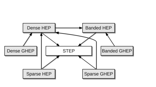
Section 2.3 is summarized in Fig. 2.1, which emphasizes the importance of the STEP in solving dense or sparse Hermitian eigenproblems. As direct methods do not exploit any sparsity of the inputs, here and in the following, the term dense eigenproblem implies the use of direct methods for its solution, i.e., the input is treated as if it were dense. Besides its importance for eigenvalue problems, the STEP is an integral part in the computation of singular value decompositions [177].

Figure 2.1: Computational paths leading to the real symmetric tridiagonal eigenproblem (STEP). Dense means that the matrix is treated as a dense matrix and a direct method is used for the solution, while sparse refers to the use of an iterative method, which are mainly used for large-scale sparse eigenproblems.

2.4 Existing software

Numerous software implements the previously described methods for the solution of eigenvalue problems. In this section, we list a few libraries – with no intention of being exhaustive.

In 1972, EISPACK [143] was released – a collection of Fortran subroutines based on the ALGOL programs by Wilkinson et al. [173]. LAPACK – first released in 1992 – superseded EISPACK and includes a number of new and improved algorithms for eigenvalue problems. Efficiency and (trans)portability is achieved by casting the computation in terms of common building blocks – the BLAS (Basic Linear Algebra Subprograms) [97, 49, 50]. BLAS are commonly provided in optimized, machine-specific form such as included in Intel’s MKL. Today, LAPACK is the most widely used numerical linear algebra library on serial and shared-memory machines; it is provided in optimized form by all major computer vendors (e.g., Intel’s MKL, IBM’s ESSL, AMD’s ACML, Sun Performance library) and commonly used through high-level interfaces (e.g., Matlab, Maple, NAG Numerical libraries). For the tridiagonal eigenproblem, LAPACK includes implementations of the four described methods (BI, DC, QR, and MRRR). In line with the discussion in Section 2.3, the tridiagonal eigensolvers form the basis of direct methods for standard and generalized Hermitian eigenproblems. A list of LAPACK’s eigensolvers relevant to this dissertation can be found in Appendix A. LAPACK does not support successive band reduction, but the corresponding routines are provided by the SBR toolbox [19] and are included in some vendor-specific LAPACK libraries. LAPACK’s support for multi-core architectures is confined to the use of multi-threaded BLAS.

A number of research efforts are currently devoted to adapt LAPACK’s functionality to multi-core and many-core processors. Among them, PLASMA [2], MAGMA [2], and FLAME [157, 158]. When this dissertation started, none of those projects included routines for the solution of eigenproblems. Recent effort changed this situation: Today, FLAME includes a solver for the HEP based on the direct reduction to tridiagonal form [160] and a QR [159] that is significantly faster than its LAPACK analog. MAGMA has support for the HEP [70, 165] and PLASMA added support for the GHEP and the HEP based on SBR [101] and QR.

Several libraries address distributed-memory architectures, including ScaLAPACK [20], PLAPACK [156], PeIGS [54, 42], PRISM [15, 16], and Elemental [128]. ScaLAPACK was introduced in 1995; its goal is to provide the same functionality as LAPACK. A list of ScaLAPACK’s eigensolvers relevant to this dissertation can be found in Appendix A. Routines for an alternative one-stage reduction and the two-stage SBR were released within the ELPA project in 2011 [9, 8]. Introduced in the 1990s was also PLAPACK, which is “an […] infrastructure for rapidly prototyping” [179] parallel algorithms and “resulted from a desire to solve the programmability crisis that faced computational scientists in the early days of massively parallel computing” [127]. For PLAPACK related to eigenproblems, see [13, 179]. As the “major development on the PLAPACK project ceased around 2000” [127], today, it is largely outdated and superseded by Elemental. Elemental is equally a framework for dense matrix computations on distributed-memory architectures. Its main objective is to ease the process of implementing matrix operations without conceding performance or scalability. Elemental includes a library for commonly used matrix operations; for standard and generalized Hermitian eigenproblems, the library includes eigensolvers based on the parallel MRRR presented in Chapter 4. More on Elemental’s eigensolvers can be found in Chapter 4.

2.5 Objectives

The ideal eigensolver is accurate, fast, scalable, and reliable. In this section, we state how to quantify these attributes. Basic definitions such as accuracy, scalability and load balancing are adopted from [114, 140].

Accuracy.

Given an Hermitian matrix $A\in\mathbb{C}^{n\times n}$ (possibly real-valued and tridiagonal) and a set of computed eigenpairs $\{(\hat{\lambda}_{i},\hat{x}_{i}):i\in\mathcal{I}\}$, $\|\hat{x}_{i}\|=1$, we quantify the results by the largest residual norm and the orthogonality, which are defined as

$$R=\max_{i}\frac{\|A\hat{x}_{i}-\hat{\lambda}_{i}\hat{x}_{i}\|_{1}}{\|A\|_{1}}\quad\mbox{and}\quad O=\max_{i}\max_{j\neq i}|\hat{x}_{i}^{*}\hat{x}_{j}|\,,$$ (2.5)

respectively. If both $R$ and $O$ are $\mathcal{O}(n\varepsilon)$, with implied constant in the hundreds, we say that the eigenpairs are computed accurately. In the following, we accept this definition of accuracy without further discussion.

The accuracy depends on a number of factors: the algorithm $\mathcal{A}$ used, a set of parameters $\mathcal{P}$ of a specific implementation of $\mathcal{A}$, and the input matrix $A$ – in particular its dimension $n$. Consequently, we have $R(\mathcal{A},\mathcal{P},n,A)$ and $O(\mathcal{A},\mathcal{P},n,A)$. From each algorithm $\mathcal{A}$, we isolate the set of parameters $\mathcal{P}$, including convergence criteria and thresholds, so that if two implementations of the same algorithm only differ in $\mathcal{P}$, then they are still considered implementations of the same algorithm.

To compare a set of algorithms, each with a fixed set of parameters, we factor in the dependence of the input matrix by obtaining results for a large set of test matrices. Ideally, such a test set would be somewhat standardized and consist of a variety of application and artificial matrices in a wide range of sizes. Taking for each size $n$ the average and worst case accuracy usually represents well the accuracy of an algorithm and gives some practical upper bounds on the residuals and orthogonality. In general, for a stable algorithm it is possible to provide theoretical error bounds, independently of all properties of the input matrix but its size. These theoretical upper bounds are essential for proving stability and for improving algorithms, but often greatly overestimate the actual error. Wilkinson wrote [171, 66], “a priori bounds are not, in general, quantities that should be used in practice. Practical error bounds should usually be determined in some form of a posteriori error analysis, since this takes full advantage of the statistical distribution of rounding error […].” In this thesis, we will evaluate and compare the accuracy of algorithms by executing them with a set of test matrices.

Speed.

Suppose we solve a fixed problem using $p$ processing units, indexed by $1\leq i\leq p$, with individual execution times $\tilde{t}_{i}$. The time to solution, $t_{p}$, is naturally defined as

$$t_{p}=\max\{\tilde{t}_{i}:1\leq i\leq p\}\,.$$ (2.6)

For different values of $p$, similar to the accuracy assessment, the average and worst case execution times on a set of test matrices can be used to compare the performance of different eigensolvers. Such an approach, with $p=1$, is taken in [37] to evaluate the performance of LAPACK’s symmetric tridiagonal eigensolvers. As the performance not only depends on the input matrices, but also on the architecture and the implementation of external libraries, an evaluation is a difficult task. In many of our experiments, not only the test set is inadequate in its generality, but also the variety of the underlying hardware is not large enough to draw final conclusions (it never is). However, from our observations, we can derive some general behavior of the different methods and their implementations.

Scalability.

For a fixed problem, let $t_{p}$ be as defined in (2.6) and let $t_{ref}$ be a reference time using $p_{ref}\leq p$ processing units. The speedup, $s_{p}$, is defined as

$$s_{p}=\frac{t_{ref}\cdot p_{ref}}{t_{p}}\,.$$ (2.7)

Usually $t_{ref}=t_{1}$ refers to the execution of the best available sequential solution and, consequently, $p_{ref}=1$. The corresponding parallel efficiency, $e_{p}$, is defined as

$$e_{p}=\frac{s_{p}}{p}=\frac{t_{ref}\cdot p_{ref}}{t_{p}\cdot p}\,.$$ (2.8)

When investigating the scalability (speedup or efficiency) for a fixed problem, we refer to strong scalability. For practical problems and values for $p$, the goal is to achieve $s_{p}\approx p$ and $e_{p}\approx 1$. If this is achieved, we say that we obtain perfect speedups or perfect scalability.

By Amdahl’s law [4], even without taking synchronization and communication cost into account, perfect speedup is not always attainable. If a fraction $f$ of a code is inherently sequential, the speedup and efficiency are limited by

$$s_{p}\leq\frac{1}{f+(1-f)/p}<\frac{1}{f}\quad\mbox{and}\quad e_{p}\leq\frac{1}{1+(p-1)f}\,.$$ (2.9)

Since always $f>0$, the efficiency eventually goes to zero as $p$ increases for any parallel code.

Besides strong scalability, we are interested in the so called weak scalability, where the number of processors is increased together with the problem size. As attested by Fred Gustafson in his article “Reevaluating Amdahl’s Law”, weak scalability has often a greater significance as in “practice, the problem size scales with the number of processors […] to make use of the increased facilities” [69]. In particular, we consider the so called memory-constraint scaling, where the amount of memory per processor is kept constant while problem size and number of processors are increased.

For weak scalability, the parallel efficiency, $\check{e}_{p}$, is defined as

$$\check{e}_{p}=\frac{e_{p}\cdot\theta}{\theta_{ref}}=\frac{t_{ref}\cdot p_{ref}\cdot\theta}{t_{p}\cdot p\cdot\theta_{ref}}\,,$$ (2.10)

where $\theta$ and $\theta_{ref}$ are measures of the work required to solve respectively the problem and the reference problem. For standard and generalized dense eigenvalue problems, we have $\theta/\theta_{ref}=n^{3}/n_{ref}^{3}$ and, for MRRR, we have $\theta/\theta_{ref}\approx n^{2}/n_{ref}^{2}$. If in an experiment $\check{e}_{p}\approx 1$, we say that we obtain perfect scalability. As with accuracy and timings, the average and worst case efficiency on a set of test matrices can be used to compare the scalability of different eigensolvers.

Load and memory balancing.

With $\tilde{t}_{i}$ as defined above, the average execution time, $\bar{t}_{p}$, is given by

$$\bar{t}_{p}=\frac{1}{p}\sum_{i=1}^{p}\tilde{t}_{i}\,.$$ (2.11)

The load balance is quantified by

$$b_{p}=\frac{\bar{t}_{p}}{\max\{\tilde{t}_{i}:1\leq i\leq p\}}\,.$$ (2.12)

An execution is called load balanced if $b_{p}\approx 1$ and unbalanced if $b_{p}\approx 0$. Using (2.8) with $t_{ref}=t_{1}$ and assuming $t_{1}\leq\sum_{i=1}^{n}\tilde{t}_{i}$, we have $e_{p}\leq b_{p}$. Consequently, without load balancing, it is not possible to achieve good parallel efficiency.

Besides a balanced workload, the total memory usage should be equally distributed among the $p$ processing units. For a specific problem, let $m$ denote the total memory requirement and let $\tilde{m}_{i}=\tilde{c}_{i}m/p$ be the memory requirement for processing unit $i$. If $c_{p}=\max\{c_{i}:1\leq i\leq p\}$ is bounded by a small constant for the tested values of $p$, we say that we achieved perfect memory balancing. Again, for a fixed problem, if $p$ increases, eventually memory balancing is lost for any parallel code. Therefore, as for the weak scaling, we often are interested in the memory balancing for problems that increase in size as the number of processors increase. For computing all eigenpairs, we have $m=\nu n^{2}$, with $\nu$ being a constant depending on the solver. Consequently, memory balancing is achieved when the maximum memory required by any processing unit,

$$m_{p}=\max\{\tilde{m}_{i}:1\leq i\leq p\}\,,$$ (2.13)

is $\mathcal{O}(n^{2}/p)$, with a small implicit constant.

Robustness.

In order to quantify the robustness of an eigensolver, we use the following measure: For a given test set of matrices, TestSet, the robustness $\phi\in[0,1]$ is expressed as

$$\phi(\mbox{\sc TestSet})=1-\frac{\mbox{\sc NumFailures}}{|\mbox{\sc TestSet}|}\,$$ (2.14)

where NumFailures is the number of inputs for which the method “fails”. We will be more concrete on what to consider failure in Chapter 5.

Chapter 3 The MRRR Algorithm

Since its introduction in the 1990s, much has been written about the MRRR algorithm; its theoretical foundation is discussed in several publications [40, 118, 43, 44, 119, 117, 164, 174, 175, 178] and practical aspects of efficient and robust implementations are discussed in [46, 45, 102, 103, 13, 162, 124, 123, 163]. In particular, Paul Willem’s dissertation [174] as well as Inderjit Dhillon’s and Beresford Parlett’s two seminal articles [43, 44] provide excellent and essential reading for everyone interested in the algorithm. One could say, with an implementation of the algorithm in the widely used LAPACK library and the description of (parts of) the algorithm in textbooks such as [168], MRRR has become mainstream.

Most publications however are either concerned about a proof of correctness or only a specific detail of the algorithm. Our description of the algorithm has a different purpose: for the non-expert, we describe the factors influencing performance, parallelism, accuracy, and robustness. We highlight the main features of the algorithm, the sources of parallelism, and the existing weaknesses. Our exposition, which is largely based on [43, 44, 174, 175], serves as a basis for the discussion in Chapters 4 and 5. We are not afraid to omit details and proofs, which can be found in other places in the literature. In contrast to Chapters 4 and 5, in this chapter we are not primarily concerned with efficiency.

The chapter is organized as follows: In Section 3.1, we give a high-level description of MRRR, with the main goal being the introduction of Algorithm 2. Furthermore, we establish the terminology and notation used in later chapters. For the discussion in Chapter 5, we present in Theorem 3.1.4 all the factors that influence the accuracy of MRRR. By fixing the form to represent tridiagonals, Section 3.2 provides a more concrete description of the computation of eigenvalues and eigenvectors. An expert of MRRR might safely skip the entire chapter and continue with Chapter 4 or 5. We recommend however to read at least Section 3.1, as it contains all the required background and notation for the later chapters.

3.1 The big picture

Consider the symmetric tridiagonal $T\in\mathbb{R}^{n\times n}$ with diagonal $a=(\alpha_{1},\ldots,\alpha_{n})$ and off-diagonal $b=(\beta_{1},\ldots,\beta_{n-1})$:

$$T=\left(\begin{array}[]{cccc}\alpha_{1}&\beta_{1}&&\\ \beta_{1}&\alpha_{2}&\ddots&\\ &\ddots&\ddots&\beta_{n-1}\\ &&\beta_{n-1}&\alpha_{n}\\ \end{array}\right)\,.$$ (3.1)

Recall that the goal is to compute a set of eigenpairs $\{(\hat{\lambda}_{i},\hat{z}_{i}):i\in\mathcal{I}\}$, $\lVert\hat{z}_{i}\rVert=1$, such that for all $i\in\mathcal{I}$

$$\lVert T\hat{z}_{i}-\hat{\lambda}_{i}\hat{z}_{i}\rVert=\mathcal{O}(n\varepsilon\lVert T\rVert)\,,$$ (3.2)

and for all $i,j\in\mathcal{I}$ with $i\neq j$

$$|\hat{z}_{i}^{*}\hat{z}_{j}|=\mathcal{O}(n\varepsilon)\,.$$ (3.3)

For now, without any loss of generality, we assume $\beta_{i}\neq 0$ for $1\leq i\leq n-1$, as otherwise the matrix is the direct sum of tridiagonals and the eigenpairs are found by inspecting each tridiagonal submatrix separately [172]. As no off-diagonal element is equals to zero, the matrix $T$ is irreducible and the following theorem holds.

Theorem 3.1.1.

The eigenvalues of an irreducible real symmetric tridiagonal matrix are simple, i.e., they are distinct. Proof: See [114].

Although the eigenvalues are distinct, they might be equal to working precision [114]. Nonetheless, distinct eigenvalues imply that each normalized eigenvector is uniquely determined up to a factor of $-1$. Consequently, if we could compute normalized eigenvectors $\hat{z}_{i}$ and $\hat{z}_{j}$, $i\neq j$, such that the (acute) error angle with the true eigenvectors are small, that is

$$\sin\angle(\hat{z}_{i},z_{i})\leq\mathcal{O}(n\varepsilon)\quad\mbox{and}\quad\sin\angle(\hat{z}_{j},z_{j})\leq\mathcal{O}(n\varepsilon)\,,$$ (3.4)

the computed eigenvectors would be numerically orthogonal:

$$|\hat{z}_{i}^{*}\hat{z}_{j}|\leq\sin\angle(\hat{z}_{i},z_{i})+\sin\angle(\hat{z}_{j},z_{j})\leq\mathcal{O}(n\varepsilon)\,.$$ (3.5)

In general, in finite precision computations, accuracy as in (3.4) is not achievable as, whenever the eigenvalues are “close” to one another, “small” perturbation in the data can lead to “large” perturbations in the eigenvectors [172, 114]. Different algorithms therefore have particular means to ensure the goal of numerical orthogonality. For example, algorithms like QR or Jacobi, which obtain eigenvector approximations by accumulating orthogonal transformations, achieve the goal automatically without (3.4) necessarily being satisfied [44]. The method of inverse iteration addresses the problem by explicitly orthogonalizing the eigenvectors corresponding to close eigenvalues (in the absolute sense) – as discussed in Section 2.3, potentially this is an expensive procedure. For Divide & Conquer and MRRR, more sophisticated techniques are used [67, 68, 43, 44]. The way the MRRR algorithm computes numerically orthogonal eigenvectors – without explicit othogonalization – is at the heart of this chapter.

In the next two sections, we illustrate the principles behind MRRR assuming exact and finite precision arithmetic, respectively. Generally, (3.4) can only be achieved in exact arithmetic, while in finite precision more effort is required to ensure orthogonality among eigenvectors.

3.1.1 Computing with exact arithmetic

In general, even when operating in exact arithmetic, there exists no procedure to compute eigenvalues of matrices in a finite number of steps, cf. [154, Theorem 25.1]. As a results, only approximations to eigenvalues and eigenvectors can be computed. In this section, we concentrate on the way approximations to eigenvectors are obtained from given approximations to eigenvalues.

First however, suppose an eigenvalue $\lambda$ is known exactly. The corresponding true eigenvector $z$ is given by

$$(T-\lambda I)z=0\,,$$ (3.6)

or, using (3.1), equally by

$$(\alpha_{1}-\lambda)z(1)+\beta_{1}z(2) =0\,,$$ (3.7a)

$$\beta_{i-1}z(i-1)+(\alpha_{i}-\lambda)z(i)+\beta_{i}z(i+1) =0\,,$$ (3.7b)

$$\beta_{n-1}z(n-1)+(\alpha_{n}-\lambda)z(n) =0\,,$$ (3.7c)

where the second equation holds for $1<i<n$. Equations (3.7) imply that $z(1)\neq 0$ and $z(n)\neq 0$ as otherwise $z=0$. Therefore, setting either $z(1)=1$ or $z(n)=1$ and using respectively the first or last $n-1$ equations yields the sought after eigenvector. Furthermore, as $T-\lambda I$ is singular, the unused equation is automatically satisfied.

Due to finiteness of any approximation procedure, even in exact arithmetic, the approximation $\hat{\lambda}$ has generally a nonzero error. (In practice, whenever we attempt to compute the corresponding eigenvector, we ensure that $\hat{\lambda}$ is closer to $\lambda$ than to any other eigenvalue.) Since $\hat{\lambda}\notin spec[T]$, $T-\hat{\lambda}I$ is nonsingular and solving in the described way for an eigenvector results in $\hat{z}$ that satisfies $(T-\hat{\lambda}I)\hat{z}=\gamma_{n}e_{n}$ or $(T-\hat{\lambda}I)\hat{z}=\gamma_{1}e_{1}$, where the scaling factor $\gamma_{k}$ takes into account that the $k$-th equation in (3.7) does not hold automatically anymore. In fact, there is nothing special about omitting the last or the first equation: we might omit the $k$-th equation for any $1\leq k\leq n$ and therefore solve $(T-\hat{\lambda}I)\hat{z}=\gamma_{k}e_{k}$. Those computations are naturally not equivalent: Omitting the $k$-th equation, $(T-\hat{\lambda}I)\hat{z}=\gamma_{k}e_{k}$, leads to $\hat{z}$ with residual norm $\lVert\bar{r}\rVert$ given by

$$\lVert\bar{r}\rVert=\frac{\lVert T\hat{z}-\hat{\lambda}\hat{z}\rVert}{\lVert\hat{z}\rVert}=\frac{|\gamma_{k}|}{\lVert\hat{z}\rVert}\,.$$ (3.8)

It has been known for a long time (see [82]) that there exists at least one index $r$ with $|z(r)|\geq n^{-1/2}$ satisfying

$$\lVert{\bar{r}}\rVert=\frac{|\gamma_{r}|}{\lVert\hat{z}\rVert}\leq\frac{|\hat{\lambda}-\lambda|}{|z(r)|}\leq\sqrt{n}|\hat{\lambda}-\lambda|\,.$$ (3.9)

Due to the inability of determining such an index $r$ cheaply, the procedure was abandoned by Wilkinson and replaced by inverse iteration using a “random” starting vector [172]. In the 1990s however, Dhillon and Parlett [118] showed – extending the work of Godunov et al. [65] and Fernando [58, 59, 57] – how to find such an index $r$. As a consequence, if $\hat{\lambda}$ is a good approximation of $\lambda$, say $|\hat{\lambda}-\lambda|=\mathcal{O}(\sqrt{n}\varepsilon\lVert T\rVert)$, the method delivers an eigenvector approximation $\hat{z}$ with a small residual norm (backward error) that satisfies (3.2). Unfortunately, if the eigenvalue is not well-separated from the rest of the spectrum, such $\hat{z}$ does not necessarily satisfy the accuracy dictated by (3.4) as the following classical theorem reveals.

Theorem 3.1.2 (Gap Theorem).

Given a symmetric matrix $T\in\mathbb{R}^{n\times n}$ and an approximation $(\hat{\lambda},\hat{z})$, $\|\hat{z}\|=1$, to the eigenpair $(\lambda,z)$, with $\hat{\lambda}$ closer to $\lambda$ than to any other eigenvalue, let $\bar{r}$ be the residual $T\hat{z}-\hat{\lambda}\hat{z}$; then

$$\sin\angle(\hat{z},z)\leq\frac{\|\bar{r}\|}{\mbox{gap}(\hat{\lambda})}\,,$$ (3.10)

with $\mbox{gap}(\hat{\lambda})=\min_{j}\{|\hat{\lambda}-\lambda_{j}|:\lambda_{j}\in spec[T]\,\wedge\,\lambda_{j}\neq\lambda\}$. The residual norm is minimized if $\hat{\lambda}$ is the Rayleigh quotient of $\hat{z}$, $\hat{\lambda}=\hat{z}^{*}T\hat{z}$. In this case,

$$\frac{\|\bar{r}\|}{spdiam[T]}\leq\sin\angle(\hat{z},z)\quad\mbox{and}\quad|\hat{\lambda}-\lambda|\leq\min\left\{\lVert\bar{r}\rVert,\frac{\lVert\bar{r}\rVert^{2}}{\mbox{gap}(\hat{\lambda})}\right\}\,.$$ (3.11)

Proof: See [114, 32, 31, 174].

Inequality (3.10) gives not only an upper bound, but also a good approximation for the error angle [115]. Therefore, by (3.9) and (3.10), we require the separation relative to $\lVert T\rVert$ to be reasonably large for (3.4) to hold, say $\mbox{gap}(\hat{\lambda})/\lVert T\rVert\geq abstol$ with $abstol\approx 10^{-3}$. On the other hand, if $\hat{\lambda}$ approximates $\lambda$ to high relative accuracy, i.e., $|\hat{\lambda}-\lambda|=\mathcal{O}(n\varepsilon|\lambda|)$, a small error angle to the true eigenvector is obtained whenever the relative gap, i.e.,

$$\mbox{relgap}(\hat{\lambda})=\mbox{gap}(\hat{\lambda})/|\lambda|$$ (3.12)

is sufficiently large, say $\mbox{relgap}(\hat{\lambda})\geq gaptol$ with $gaptol\approx 10^{-3}$. Thus, given approximations to the desired eigenvalues to high relative accuracy, the above procedure allows to compute an accurate eigenvector whenever the relative gap of the eigenvalue is large.

Assuming we have approximated the desired eigenvalues $\{\hat{\lambda}_{i}:i\in\mathcal{I}\}$ to high relative accuracy, whenever $\mbox{relgap}(\hat{\lambda}_{i})\geq gaptol$, we compute eigenvector $\hat{z}_{i}$ with a small error angle. In practice, we are slightly more restrictive on when to compute an eigenvector; at this point of the discussion, this detail is not important and we will return to this matter later. If our (slightly adjusted) criterion indicates that we can compute the eigenvector with a small error angle, $\hat{\lambda}_{i}$ is said to be well-separated, isolated, or a singleton. For all well-separated eigenvalues, we can independently compute the corresponding eigenvectors so that all resulting eigenpairs satisfy our accuracy goals given by (3.2) and (3.3).

Input: Irreducible symmetric tridiagonal $T\in\mathbb{R}^{n\times n}$; index set $\mathcal{I}_{in}\subseteq\{1,\ldots,n\}$.
Output: Eigenpairs $(\hat{\lambda}_{i},\hat{z}_{i})$ with $i\in\mathcal{I}_{in}$.

1:  Compute $\hat{\lambda}_{i}[T]$ with $i\in\mathcal{I}_{in}$ to high relative accuracy.

2:  Form a work queue $Q$ and enqueue task $\{T,\mathcal{I}_{in},0\}$.

3:  while $Q$ not empty do

4:       Dequeue a task $\{M,\mathcal{I},\sigma\}$.

5:       Partition $\mathcal{I}=\bigcup_{s=1}^{S}\mathcal{I}_{s}$ according to the separation of the eigenvalues.

6:       for $s=1$ to $S$ do

7:             if $\mathcal{I}_{s}=\{i\}$ then

8:                  // process well-separated eigenvalue associated with singleton $\mathcal{I}_{s}$ //

9:                  Solve $(M-\hat{\lambda}_{i}[M]I)\hat{z}_{i}=\gamma_{r}e_{r}$ with appropriate index $r$ for $\hat{z}_{i}$.

10:                  Return $\hat{\lambda}_{i}[T]=\hat{\lambda}_{i}[M]+\sigma$ and normalized $\hat{z}_{i}$.

11:             else

12:                  // process cluster associated with $\mathcal{I}_{s}$ //

13:                  Select shift $\tau\in\mathbb{R}$ and compute $M_{shifted}=M-\tau I$.

14:                  Refine $\hat{\lambda}_{i}[M_{shifted}]$ with $i\in\mathcal{I}_{s}$ to high relative accuracy.

15:                  Enqueue $\{M_{shifted},\mathcal{I}_{s},\sigma+\tau\}$.

16:             end if

17:       end for

18:  end while

Algorithm 1  MRRR using exact arithmetic

If some eigenvalues are non-isolated, they come in collections of two or more consecutive values, say $\{\hat{\lambda}_{p}[T],\hat{\lambda}_{p+1}[T]\ldots,\hat{\lambda}_{q}[T]\}$. These collections are called clusters and the eigenvalues are said to be clustered. To compute the eigenvectors for clusters, the following observation is used: the eigenvectors are invariant under shifts (i.e., forming $T-\tau I$ for some $\tau\in\mathbb{R}$), while the relative gaps are not. Indeed, by choosing $\tau$ to be (close to) one eigenvalue, say $\tau=\hat{\lambda}_{p}[T]$, one can decrease the magnitude of this eigenvalue and therefore increase its relative gap:

$$\mbox{relgap}(\hat{\lambda}_{p}[T-\tau I])=\mbox{relgap}(\hat{\lambda}_{p}[T])\frac{|\lambda_{p}[T]|}{|\lambda_{p}[T]-\tau|}\gg\mbox{relgap}(\hat{\lambda}_{p}[T])\,.$$ (3.13)

In exact arithmetic, there exists a shift $\tau$ to make the relative gap as large as desired; in particular, we can make the eigenvalue well-separated with respect to the shifted matrix $T-\tau I$. Using $T-\tau I$, for all those eigenvalues of the original cluster that are now well-separated, we then compute the eigenvectors with small error angle to the corresponding true eigenvectors. For the eigenvalues that are still clustered, we apply the procedure recursively until we have computed all eigenvectors. The overall procedure is summarized in Algorithm 1.

3.1.2 Computing with finite precision arithmetic

While the procedure described above sounds seemingly simple, there are several obstacles when applied in finite precision arithmetic. Most notably, the invariance of the eigenvectors under shifts is lost. Furthermore, rounding errors could spoil the computation of an eigenvector in Line 9 of Algorithm 1. Finally, we have not specified how the so called twist index $r$ is chosen in exact arithmetic and this task might be impossible in finite precision or computationally expensive. In this section, we give an overview of how these problems are addressed. The ideas were developed in [40, 43, 44, 119, 174, 178, 176, 175] and realized the above procedure in floating point arithmetic – today known as the algorithm of Multiple Relatively Robust Representations.

Change of representation.

Small element-wise relative perturbations of the diagonal and off-diagonal entries of $T$ can lead to large relative perturbations of small (in magnitude) eigenvalues [44, 115]. In such a case, it is said that the data does not define these eigenvalues to high relative accuracy. As a consequence, using finite precision arithmetic, we cannot hope to compute eigenvalues to high relative accuracy. In order for the procedure of Algorithm 1 to work, the representation of tridiagonals by their diagonal and off-diagonal entries must be abandoned and alternative representations must be used. To discuss these alternatives, we give a general definition of the concept of a representation first.

Definition 3.1.1 (Representation).

A set of $2n-1$ scalars, called the data, together with a mapping $f:\mathbb{R}^{2n-1}\rightarrow\mathbb{R}^{2n-1}$ to define the entries of a symmetric tridiagonal matrix $T\in\mathbb{R}^{n\times n}$ is called a representation of $T$ [175].

According to the above definition, the set containing the diagonal and off-diagonal entries together with the identity mapping is a representation of a tridiagonal. Unfortunately, such a representation generally does not have desirable properties under small element-wise relative perturbations. As all perturbations in this chapter are element-wise and relative, we sometimes omit these attributes for the sake of brevity.

Definition 3.1.2 (Perturbation of a representation).

Let $x_{1},\ldots,x_{2n-1}$ be the scalars used to represent the symmetric tridiagonal $T\in\mathbb{R}^{n\times n}$ and $\tilde{x}_{i}=x_{i}(1+\xi_{i})$ be relative perturbations of them; using the same representational mapping as for $T$, they define a matrix $\widetilde{T}$. If $\xi_{i}\leq\xi\ll 1$ for all $1\leq i\leq 2n-1$, we call $\widetilde{T}$ a small perturbation of $T$ bounded by $\xi$ [175].

We are interested in representations that have the property that small perturbations cause small perturbations in some of the eigenvalues and eigenvectors. Such a representation is called relatively robust and constitutes a relatively robust representation (RRR). As the definition of relative robustness – given below – requires the notion of a relative gap connected to an index set $\mathcal{I}\subset\{1,\ldots,n\}$, we define such a relative gap first.

Definition 3.1.3.

Given a symmetric $T\in\mathbb{R}^{n\times n}$ with simple eigenvalues $\{\lambda_{i}:1\leq i\leq n\}$ and an index set $\mathcal{I}\subset\{1,\ldots,n\}$, the relative gap connected to $\mathcal{I}$ is defined as

$$\mbox{\em relgap}(\mathcal{I})=\min\left\{\frac{|\lambda_{j}-\lambda_{i}|}{|\lambda_{i}|}:i\in\mathcal{I},j\notin\mathcal{I}\right\}$$

where $|\lambda_{j}-\lambda_{i}|/|\lambda_{i}|$ is $\infty$ if $\lambda_{i}=0$ [43].

Definition 3.1.4 (Relative robustness).

Given a representation of the irreducible symmetric tridiagonal $T\in\mathbb{R}^{n\times n}$ and an index set $\mathcal{I}\subset\{1,\ldots,n\}$, we say that the representation is relatively robust for $\mathcal{I}$ if for all small perturbations $\widetilde{T}$ bounded by $\xi$ and $i\in\mathcal{I}$, we have

$$|\tilde{\lambda}_{i}-\lambda_{i}| \leq k_{rr}n\xi|\lambda_{i}|\,,$$

$$\sin\angle(\tilde{\mathcal{Z}}_{\mathcal{I}},\mathcal{Z}_{\mathcal{I}}) \leq\frac{k_{rr}n\xi}{\mbox{\em relgap}(\mathcal{I})}\,,$$

where $\tilde{\lambda}_{i}$ and $\tilde{\mathcal{Z}}_{\mathcal{I}}$ denote the eigenvalues and the corresponding invariant subspaces of the perturbed matrices, respectively, and $\angle(\tilde{\mathcal{Z}}_{\mathcal{I}},\mathcal{Z}_{\mathcal{I}})$ the largest principle angle [66]; $k_{rr}$ is a moderate constant, say about 10 [43, Property I].

We say that an RRR for $\{i\}$ is relatively robust for the eigenpair $(\lambda_{i},z_{i})$, or alternatively, that such an RRR defines the eigenpair to high relative accuracy. As we will see later, when using suitable representations and algorithms, the matrix shifts performed in Line 13 of Algorithm 1, $M_{shifted}=M-\tau I$, introduce small relative perturbations in the data of $M$ and $M_{shifted}$. In order for those perturbations not to influence too much the invariant subspace $\mathcal{Z}_{\mathcal{I}_{s}}$ associated to a cluster, we must modify Algorithm 1 in such a way that $M$ and $M_{shifted}$ are RRRs for $\mathcal{I}_{s}$. Similarly, in order to compute a highly accurate eigenpair, we need a representation that defines the eigenpair to high relative accuracy. Thus, we have to replace the original $T$ with a suitable initial or root representation $M_{root}=T-\mu I$ for some $\mu\in\mathbb{R}$ and carefully select every intermediate representation, $M_{shifted}$, that is computed in Line 13 of Algorithm 1.

There are multiple candidates – existence assumed – for playing the role of RRRs, which often but not always are relatively robust for index sets connected to small eigenvalues (in magnitude) and the associated invariant subspaces:

1. Lower bidiagonal factorizations of the form $T=LDL^{*}$ and upper bidiagonal factorizations of the form $T=U\Omega U^{*}$, where $D=\mbox{diag}(d_{1},d_{2},\ldots,d_{n})\in\mathbb{R}^{n\times n}$ and $\Omega=\mbox{diag}(\omega_{1},\omega_{2},\ldots,\omega_{n})\in\mathbb{R}^{n\times n}$ are diagonal, $L\in\mathbb{R}^{n\times n}$ and $U\in\mathbb{R}^{n\times n}$ are respectively unit lower bidiagonal and unit upper bidiagonal, i.e.,

   $$\small L=\left(\begin{array}[]{cccccc}1&&&&\\ \ell_{1}&1&&&\\ &\ell_{2}&1&&\\ &&\ddots&\ddots&\\ &&&\ell_{n-1}&1\\ \end{array}\right)\quad\mbox{and}\quad U=\left(\begin{array}[]{cccccc}1&u_{1}&&&\\ &1&u_{2}&&\\ &&1&\ddots&\\ &&&\ddots&u_{n-1}\\ &&&&1\\ \end{array}\right)\,.$$

   Lower bidiagonal factorizations were used to represent the intermediate tridiagonal matrices ($M$ in Algorithm 1) in the original implementations of the algorithm [40, 46]. In the definite case, i.e., $|D|=\pm D$ or $|\Omega|=\pm\Omega$, a bidiagonal factorization is an RRR for all eigenpairs [36]. Therefore, such a definite factorization is often used as an initial representation $M_{root}=T-\mu I$.

2. A generalization of the above are so called twisted factorizations or BABE-factorizations [57, 118] of the form $T=N_{k}\Delta_{k}N_{k}^{*}$, where $k$ denotes the twist index. $N_{k}$ has the form

   $$\small N_{k}=\left(\begin{array}[]{ccccccc}1&&&&&&\\ \ell_{1}&1&&&&&\\ &\ddots&\ddots&&&&\\ &&\ell_{k-1}&1&u_{k}&&\\ &&&&\ddots&\ddots&\\ &&&&&1&u_{n-1}\\ &&&&&&1\\ \end{array}\right)\,,$$ (3.14)

   and $\Delta_{k}=\mbox{diag}(d_{1},\ldots,d_{k-1},\gamma_{k},\omega_{k+1},\ldots,\omega_{n})$ is diagonal. The factorizations for all $1\leq k\leq n$ are almost entirely defined by elements of the bidiagonal factorizations $T=LDL^{*}=U\Omega U^{*}$; only $\gamma_{k}$, $1<k<n$, has to be computed. There are multiple formulations for $\gamma_{k}$, see [118, Corollary 4]; one of them is: $\gamma_{k}=d_{k}+\omega_{k}-\alpha_{k}$. Twisted factorizations are crucial in computing accurate eigenvectors in Line 9 of Algorithm 1 [118, 44]. Although it was known that these factorizations can additionally serve as representations of tridiagonals [40, 44, 117, 115], their benefits were only demonstrated recently [174, 178]. Due to their additional degree of freedom in choosing $k$, the use of twisted factorizations, which includes the bidiagonal factorizations as special cases, is superior to using only lower bidiagonal factorizations.
   

3. Blocked factorizations [55, 176] are further generalizations of bidiagonal and twisted factorizations. The quantities $D$, $\Omega$, and $\Delta_{k}$ are allowed to be block diagonal with blocks of size $1\times 1$ or $2\times 2$. The other factors – $L$, $U$, and $N_{k}$ – are partitioned conformally with one or the $2\times 2$ identity on the diagonal. These class of factorizations contain the unblocked bidiagonal and twisted factorizations as special cases. With their great flexibility, these factorizations have been used very successfully within the MRRR algorithm [174, 176].

All factorizations are determined by $2n-1$ scalars, the data; the same number as for $T$ given by its diagonal and off-diagonal elements. Through the mapping determined by the factorization, they define a tridiagonal. For instance, for lower bidiagonal factorizations, $2n-1$ floating point numbers $d_{1},\ldots,d_{n},\ell_{1},\ldots,\ell_{n-1}$ determine a tridiagonal that is generally not exactly representable in the same finite precision. Such representation by the non-trivial entries of the factorization is called an $N$-representation [178]. Similarly, the floating point numbers $d_{1},\ldots,d_{n},\beta_{1},\ldots,\beta_{n-1}$ – with $\beta_{i}=d_{i}\ell_{i}$ being $T$’s off-diagonal elements – represent a tridiagonal whose diagonal entries are in general not representable. Such representation, which includes $T$’s off-diagonal elements, is called an $e$-representation [178]. It is important to distinguish between the tridiagonal – not necessarily machine representable – and the finite precision scalars that constitute the representation. The $2n-1$ scalars constituting the representation are called the primary data. Other quantities that are computed using the primary data are called secondary or derived data. For instance, the off-diagonal $\beta_{i}=d_{i}\ell_{i}$ is secondary for an $N$-representation while being primary for an $e$-representation. Subsequently, we do not distinguish between the representation of a tridiagonal and the tridiagonal itself; that is, it is always implied that tridiagonals are represented in one of the above forms. More on different forms of representing tridiagonals can be found in [40, 115, 174, 178, 176].

It is not at all obvious that these representations are more suitable for computations than the standard way of representing tridiagonals. This is the topic of the relative perturbation theory covered in [117, 119, 44, 40], which shows how sensitive individual eigenvalues and eigenvectors are under relative component-wise perturbations.

Shifting the spectrum.

In exact arithmetic, shifting the spectrum, as in Line 13 of Algorithm 1, leaves the eigenvectors unchanged; this invariance is lost in finite precision. An essential ingredient of MRRR is the use of special forms of Rutishauser’s Quotienten-Differenzen (qd) algorithm [135, 60, 44] to perform the spectrum shifts. Given representation $M$, we require that $M_{shifted}=M-\tau I$ is computed in a element-wise mixed relative stable way, i.e., $\widetilde{M}_{shifted}=\widetilde{M}-\tau I$ holds exactly for small perturbations of $M_{shifted}$ and $M$ bounded by $\xi_{\uparrow}=\mathcal{O}(\varepsilon)$ and $\xi_{\,\downarrow}=\mathcal{O}(\varepsilon)$, respectively. In the following, we assume $\xi_{\uparrow}$ and $\xi_{\,\downarrow}$ are bounds for all spectrum shifts performed during an execution of the algorithm.

Since both $M_{shifted}$ and $M$ in Line 13 of Algorithm 1 can take any of the discussed forms, these leads to a variety of (similar) algorithms with different characteristics. For instance, using lower bidiagonal factorizations to represent intermediate matrices, we require to perform $L_{+}D_{+}L_{+}^{*}=LDL^{*}-\tau I$. This can be accomplished by the so called differential form of the stationary qd transformation (dstqds) given in Algorithm 5 [40, 44]. Similarly, using twisted factorizations, we require an algorithm that is stable in the above sense to compute $N_{t}\Delta_{t}N_{t}^{*}=N_{s}\Delta_{s}N_{s}^{*}-\tau I$ for arbitrary twist indices $s$ and $t$ [178]; the same is true for blocked factorizations [176].

In Algorithm 1, provided that $M_{shifted}$ and $M$ are relatively robust for $\mathcal{I}_{s}$ and $\mbox{relgap}(\mathcal{I}_{s})\geq gaptol$, the mixed stability implies that invariant subspaces connected to clusters are not perturbed too much due to rounding errors, $\sin\angle(\mathcal{Z}_{\mathcal{I}_{s}}[M_{shifted}],\mathcal{Z}_{\mathcal{I}_{s}}[M])\leq k_{rr}n(\xi_{\,\downarrow}+\xi_{\uparrow})/gaptol$. After the shifting, we can therefore hope to compute an orthonormal basis for such a subspace, which is automatically numerically orthogonal to the subspace spanned by the other computed eigenvectors. This is one of the main ideas behind MRRR.

The special computation of the spectrum shifts is essential for eigenvectors computed from different representations to be numerically orthogonal. In order to ensure that the eigenpairs also enjoy small residual norms with respect to the input matrix, the intermediate representations should additionally exhibit the so called conditional element growth.

Definition 3.1.5 (Conditional element growth).

A representation $M$ exhibits conditional element growth for $\mathcal{I}\subset\{1,2,\ldots,n\}$ if for any small perturbation $\widetilde{M}$ bounded by $\xi$ and $i\in\mathcal{I}$

$$\lVert\widetilde{M}-M\rVert \leq\mbox{\em spdiam}[M_{root}]\,,\quad\mbox{and}$$

$$\lVert(\widetilde{M}-M)\hat{z}_{i}\rVert \leq k_{elg}n\xi\cdot\mbox{\em spdiam}[M_{root}]\,,$$

where $\hat{z}_{i}$ denote the computed eigenvectors and $k_{elg}$ is a moderate constant, say about 10 [43, 175].

In particular, $M_{shifted}$, computed in Line 13 of Algorithm 1, needs to exhibit conditional element growth for $\mathcal{I}_{s}$. At this point, we are not concerned about how to ensure that the involved representations satisfy the requirements; this is the topic of [117, 119, 44, 175]. We remark however that there exist the danger that no suitable representation that passes the test ensuring the requirements is found. In this case, commonly a promising representation is selected. As such a representation might not fulfill the requirements, the accuracy of MRRR is not guaranteed anymore.

Independently of the form to represent the intermediate tridiagonals, the computation of twisted factorizations is essential for finding an eigenvector. Therefore, the possibility of computing twisted factorizations $N_{k}\Delta_{k}N_{k}^{*}=M-\tau I$ for $1\leq k\leq n$ must be provided for any representation used for $M$. This means we must be able to compute the lower bidiagonal factorization $L_{+}D_{+}L_{+}^{*}=M-\tau I$, the upper bidiagonal factorization $U_{-}\Omega_{-}U_{-}^{*}=M-\tau I$ and the $\gamma_{k}$ terms in a stable way in order for rounding errors not to spoil the computation of an eigenvector [44, 178].

Using twisted factorizations to find an eigenvector.

At the moment we attempt to compute an accurate eigenvector approximation $\hat{z}_{i}$ in Line 9 of Algorithm 1, we have given an RRR for $\{i\}$ and $\hat{\lambda}_{i}$ – an approximation to $\lambda_{i}$ with high relative accuracy. Furthermore, the relative gap is sufficiently large, $\mbox{relgap}(\hat{\lambda}_{i})\geq gaptol$. This special situation is analyzed in [44, 118].

Suppose $M-\hat{\lambda}_{i}I=L_{+}D_{+}L_{+}^{*}=U_{-}\Omega_{-}U_{-}^{*}$ permits lower and upper bidiagonal factorization. We can determine all the twisted factorizations $N_{k}\Delta_{k}N_{k}^{*}=M-\hat{\lambda}_{i}I$ cheaply by computing the missing $\gamma_{k}$ for $1<k<n$. The computation must however be done with care, i.e., in a element-wise mixed relative stable way [44, 178].

When solving $(M-\hat{\lambda}_{i}I)\hat{z}_{i}=N_{k}\Delta_{k}N_{k}^{*}\hat{z}_{i}=\gamma_{k}e_{k}$, by (3.9), in exact arithmetic, the residual norm is given by $|\gamma_{k}|/\lVert\hat{z}_{i}\rVert$. Thus, a natural choice for the twist index is $r=\operatorname*{arg\,min}_{k}|\gamma_{k}|$, which is indeed used in practice. This is justified as follows: Since $|\gamma_{k}|/\lVert\hat{z}_{i}\rVert\leq|\hat{\lambda}_{i}-\lambda_{i}|/|z_{i}(k)|$ for all $1\leq k\leq n$ with $z_{i}(k)\neq 0$, see [40, Theorem 3.2.3], finding an $|z_{i}(k)|\geq n^{-1/2}$, i.e., an entry of the true eigenvector that is above average in magnitude, results in the desired bound of (3.9). As in the limiting case $\hat{\lambda}_{i}\rightarrow\lambda_{i}$,

$$\frac{\gamma_{k}^{-1}}{\sum_{j=1}^{n}{\gamma_{j}^{-1}}}\rightarrow z_{i}(k)^{2}\,,$$

provided $\hat{\lambda}_{i}$ is an accurate eigenvalue approximation, $r=\operatorname*{arg\,min}_{k}|\gamma_{k}|$ implies $|z_{i}(r)|$ is above average, see [40, Lemma 3.2.1] or [118, Lemma 11].

After finding $r$ and its associated twisted factorization, the following system needs to be solved

$$N_{r}\Delta_{r}N_{r}^{*}\hat{z}_{i}=\gamma_{r}e_{r}\Longleftrightarrow N_{r}^{*}\hat{z}_{i}=e_{r}\,,$$ (3.15)

where the equivalence stems from the fact that $N_{r}^{-1}e_{r}=e_{r}$ and $\Delta_{r}e_{r}=\gamma_{r}e_{r}$. This system is easily solved by setting $\hat{z}_{i}(r)=1$ and

$$\hat{z}_{i}(j)=\left\{\begin{array}[]{l l}-\ell^{+}_{j}\hat{z}_{i}(j+1)&\quad\text{for $j=r-1,\ldots,1$}\,,\\ -u_{j-1}^{-}\hat{z}_{i}(j-1)&\quad\text{for $j=r+1,\ldots,n$}\,.\\ \end{array}\right.$$

Finally, $\hat{\lambda}_{i}$ might be improved by the Rayleigh quotient correction term $\gamma_{r}/\lVert\hat{z}_{i}\rVert^{2}$, and finally $\hat{z}_{i}$ is normalized and returned. A more careful implementation of the procedure, taking into account possible breakdown due to finite precision arithmetic, is given in Algorithm 7 and discussed in the next section. For the sake of brevity, we neglect this issue at this point of the discussion.

The above procedure of computing an eigenvector approximation using a twisted factorization is called Getvec. A rigorous analysis of Getvec in [44], which takes all effects of finite precision into account, reveals that the computed eigenvector $\hat{z}_{i}$ has a small error angle to the true eigenvector $z_{i}$.

Theorem 3.1.3.

Suppose $\hat{z}_{i}$ is computed by Getvec under the conditions stated above. For a small perturbation of $M$ bounded by $\alpha=\mathcal{O}(\varepsilon)$, $\widetilde{M}$, and a small element-wise relative perturbation of $\hat{z}_{i}$ bounded by $\eta=\mathcal{O}(n\varepsilon)$, $\tilde{z}_{i}$, the residual norm satisfies

$$\lVert\bar{r}^{(local)}\rVert=\lVert\widetilde{M}\tilde{z}_{i}-\hat{\lambda}_{i}\tilde{z}_{i}\rVert\leq k_{rs}gap(\hat{\lambda}_{i}[\widetilde{M}])n\varepsilon/gaptol\,,$$ (3.16)

where $k_{rs}=\mathcal{O}(1)$. In this case,

$$\sin\angle(\hat{z}_{i},z_{i})\leq k_{rr}n\alpha/gaptol+k_{rs}n\varepsilon/gaptol+\eta=\mathcal{G}n\varepsilon\,,$$

where $k_{rr}$ is given by the relative robustness of $M$ for $\{i\}$ and $\mathcal{G}$ is defined by the equation. Proof: See [44].

As we have seen in (3.4) and (3.5), the small error angle, $\sin\angle(\hat{z}_{i},z_{i})\leq\mathcal{G}n\varepsilon=\mathcal{O}(n\varepsilon/gaptol)$, is essential for computing numerically orthogonal eigenvectors without explicit orthogonalization.

A high-level view and the representation tree.

Although most parts of the procedure deserve a more detailed discussion, we can now apply all the changes to Algorithm 1 to obtain a high-level view of the so called core MRRR algorithm working on irreducible tridiagonals. The whole procedure is assembled in Algorithm 2.

Input: Irreducible symmetric tridiagonal $T\in\mathbb{R}^{n\times n}$; index set $\mathcal{I}_{in}\subseteq\{1,\ldots,n\}$.
Output: Eigenpairs $(\hat{\lambda}_{i},\hat{z}_{i})$ with $i\in\mathcal{I}_{in}$.

1:  Select shift $\mu\in\mathbb{R}$ and compute $M_{root}=T-\mu I$.

2:  Perturb $M_{root}$ by a “random” relative amount bounded by a small multiple of $\varepsilon$.

3:  Compute $\hat{\lambda}_{i}[M_{root}]$ with $i\in\mathcal{I}_{in}$ to relative accuracy sufficient for classification.

4:  Form a work queue $Q$ and enqueue task $\{M_{root},\mathcal{I}_{in},\mu\}$.

5:  while $Q$ not empty do

6:       Dequeue a task $\{M,\mathcal{I},\sigma\}$.

7:       Partition $\mathcal{I}=\bigcup_{s=1}^{S}\mathcal{I}_{s}$ according to the separation of the eigenvalues.

8:       for $s=1$ to $S$ do

9:             if $\mathcal{I}_{s}=\{i\}$ then

10:                  // process well-separated eigenvalue associated with singleton $\mathcal{I}_{s}$ //

11:                  Refine $\hat{\lambda}_{i}[M]$ to high relative accuracy.

12:                  Find twisted factorization $N_{r}\Delta_{r}N_{r}^{*}=M-\hat{\lambda}_{i}[M]I$ and solve $N_{r}^{*}\hat{z}_{i}=e_{r}$ for $\hat{z}_{i}$.

13:                  Return $\hat{\lambda}_{i}[T]:=\hat{\lambda}_{i}[M]+\sigma$ and normalized $\hat{z}_{i}$.

14:             else

15:                  // process cluster associated with $\mathcal{I}_{s}$ //

16:                  Select shift $\tau\in\mathbb{R}$ and compute $M_{shifted}=M-\tau I$.

17:                  Refine $\hat{\lambda}_{i}[M_{shifted}]$ with $i\in\mathcal{I}_{s}$ to sufficient relative accuracy.

18:                  Enqueue $\{M_{shifted},\mathcal{I}_{s},\sigma+\tau\}$.

19:             end if

20:       end for

21:  end while

Algorithm 2  MRRR

Most notably, tridiagonal matrices are replaced by representations of tridiagonals, i.e., the tridiagonals are given only implicitly. These representations are required to exhibit conditional element growth and be relatively robust, which is reflected in the name of the algorithm. In Line 2, we added a small random perturbation of the root representation. Such a perturbation is crucial to break very tight clusters [45].

The unfolding of Algorithm 2 is best described as a rooted tree, the so called representation tree [40, 43, 175]. Each task $\{M,\mathcal{I},\sigma\}$ (or just $\{M,\mathcal{I}\}$) is connected to a node in the tree; that is, all of the nodes consist of a representation and an index set. The index set corresponds to the indices of all eigenpairs computed from the representation. The node $\{M_{root},\mathcal{I}_{in}\}$ is the root node (hence the name). The other tasks, $\{M,\mathcal{I}\}$, are connected to ordinary nodes. Each node has a depth – the number of edges on the unique path from the root to it. The maximum depth for all nodes (i.e., the height of the tree) is denoted $d_{max}$. The edges connecting nodes are associated with the spectrum shifts $\tau$ that are performed in Line 16 of Algorithm 2.

The concept is best illustrated by an example such as in Fig. 3.1, where $\mathcal{I}_{in}=\{1,2,\ldots,9\}$.

Figure 3.1: An exemplary representation tree.

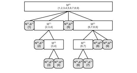
The root consists of $M_{root}=M^{(0)}$ together with $\mathcal{I}_{in}$. Ordinary nodes, which are colored in white, correspond to clustered eigenvalues with respect to the parent representation. Eigenvalues $\{\hat{\lambda}_{2}[M^{(0)}],\hat{\lambda}_{3}[M^{(0)}],\hat{\lambda}_{4}[M^{(0)}]\}$ and $\{\hat{\lambda}_{6}[M^{(0)}],\hat{\lambda}_{7}[M^{(0)}],\hat{\lambda}_{8}[M^{(0)}],\hat{\lambda}_{9}[M^{(0)}]\}$ form clusters and the first invocation of Line 7 in Algorithm 2 partitions the input index set as follows: $\mathcal{I}_{in}=\{1\}\cup\{2,3,4\}\cup\{5\}\cup\{6,7,8,9\}$. For both clusters, a new representation is computed – i.e., $M^{(1)}=M^{(0)}-\tau^{(1)}I$ and $M^{(2)}=M^{(0)}-\tau^{(2)}I$. Although in the definition of $d_{max}$ they are not counted nodes, singletons $\{i\}$ (that is, well-separated eigenvalues with respect the parent representation) are associated with leaves of the tree. For each eigenpair there exists exactly one associated leaf. For instance, $\hat{\lambda}_{1}[M^{(0)}]$ is well-separated, and the corresponding eigenpair can be computed following Lines 11–13 of Algorithm 2, which require the twisted factorization $N^{(1)}\Delta^{(1)}(N^{(1)})^{*}=M^{(0)}-\hat{\lambda}_{1}[M^{(0)}]I$. According to our definition, which excludes leaves from the definition of nodes, $d_{max}$ is two. In [40, 43] $d_{max}$ is defined differently: according to their definition, $d_{max}$ would be three. Besides for the definition of $d_{max}$, from now on, we consider leaves as nodes of the representation tree as well.

The tree of Fig. 3.1 illustrates sources of natural parallelism: All the singletons as well as clusters with the same depth in the tree can be processed independently. As an example, given $M^{(0)}$, eigenpairs $(\hat{\lambda}_{1},\hat{z}_{1})$ and $(\hat{\lambda}_{5},\hat{z}_{5})$ can be computed in parallel. At the same time, we can independently process the clusters associated with $\{2,3,4\}$ and $\{6,7,8,9\}$. When clusters are present, the computation of the eigenpairs is not independent and the amount of work associated to each eigenpair varies. If the work of computing a set of eigenpairs is divided statically by assigning a subset of indices to each processing unit, the presence of large clusters leads to load imbalance and limits scalability. Only if all the eigenvalues are well-separated with respect to the root representation, the computation of the eigenpairs is embarrassingly parallel.

Accuracy of MRRR.

As the eigenpairs are computed using possibly different representations, the main concern of the error analysis given in [43, 44, 175] is if the resulting eigenpairs enjoy small residual norm with respect to the input matrix and are mutually numerically orthogonal. The elegant analysis in [175] – a streamlined version of the proofs in [43, 44] – shows that, provided the algorithm finds suitable representations, this is indeed the case. For our discussion in Chapter 5, in following theorem we state the upper bounds on the residual norm and the orthogonality.

Theorem 3.1.4 (Accuracy).

Let $\hat{\lambda}_{i}[M_{root}]$ be computed (exactly) by applying the spectrum shifts to $\hat{\lambda}_{i}[M]$ obtained in Line 11 of Algorithm 2. Provided all the requirements of the MRRR algorithm are satisfied (in particular, that suitable representations are found), we have

$$\lVert M_{root}\,\hat{z}_{i}-\hat{\lambda}_{i}[M_{root}]\,\hat{z}_{i}\rVert\leq\left(\lVert\bar{r}^{(local)}\rVert+\gamma\,spdiam[M_{root}]\right)\frac{1+\eta}{1-\eta}$$ (3.17)

with $\lVert\bar{r}^{(local)}\rVert$ being bounded by Theorem 3.1.3 and $\gamma=k_{elg}n\left(d_{max}(\xi_{\,\downarrow}+\xi_{\uparrow})+\alpha\right)+2(d_{max}+1)\eta$. Furthermore, we have for any computed eigenvectors $\hat{z}_{i}$ and $\hat{z}_{j}$, $i\neq j$,

$$|\hat{z}_{i}^{*}\hat{z}_{j}|\leq 2\left(\mathcal{G}n\varepsilon+\frac{k_{rr}n(\xi_{\,\downarrow}+\xi_{\uparrow})d_{max}}{gaptol}\right)\,.$$ (3.18)

where $\mathcal{G}n\varepsilon=k_{rr}n\alpha/gaptol+k_{rs}n\varepsilon/gaptol+\eta$. Proof: See [174, 175] or [43, 44].

We give a number of remarks regarding the theorem:

1. The theorem hinges on the fact that suitable representations are found. If we accept one or more representations for which conditional element growth and relative robustness (i.e., being an RRR) is not verified, the accuracy of the result is not guaranteed.

2. For a reasonable implementation, we have $\alpha=\mathcal{O}(\varepsilon)$, $\eta=\mathcal{O}(n\varepsilon)$, $\xi_{\,\downarrow}=\mathcal{O}(\varepsilon)$, and $\xi_{\uparrow}=\mathcal{O}(\varepsilon)$. Furthermore, $k_{rr}$, $k_{rs}$, and $k_{elg}$ can be bounded by a small constant, say 10.

3. The assumption that the accumulation of the shifts is done in exact arithmetic is not crucial; we simply stated the theorem as in [174, 175].

4. Provided the computation $M_{root}=T-\mu I$ is performed in a backward stable manner, i.e., $M_{root}=T+\Delta T-\mu I$ with $\lVert\Delta T\rVert=\mathcal{O}(n\epsilon\lVert T\rVert)$, small residual norms with respect to the root representation, as given in (3.17), imply small residual norms to the level dictated by (3.2) [40].

5. Instead of accumulating the shifts to obtain the eigenvalues, the Rayleigh quotient of $\hat{z}_{i}$ might be returned as the corresponding eigenvalue $\hat{\lambda}_{i}$.

6. Element-wise mixed relative stability for the shifts are key to success and imply that $\xi_{\,\downarrow}=\mathcal{O}(\varepsilon)$ and $\xi_{\uparrow}=\mathcal{O}(\varepsilon)$.

7. Relative robustness of the representations is essential and is exposed by the multiple appearances of $k_{rr}$ in (3.17) (together with Theorem 3.1.3) and (3.18). The first appearance in (3.18), together with the stable spectrum shifts, indicates that invariant subspaces connected to clusters are not perturbed too much. The second appearance in (3.18) allows the computation of an eigenvector with small error angle to the true eigenvector.

8. If $\mbox{relgap}(\hat{\lambda})$ is almost as small as $gaptol$, high relative accuracy of the eigenvalue approximation is necessary. If $\mbox{relgap}(\hat{\lambda})\gg gaptol$, the accuracy of the eigenvalue approximation can be relaxed [46].

9. Large relative gaps of the clusters and well-separated eigenvalues are crucial for obtaining orthogonal eigenvectors; this is reflected in the dependence on $gaptol$ in (3.17) and (3.18).

10. Shallow representation trees (that is, small values of $d_{max}$) are preferable over deep trees. In the optimal scenario of $d_{max}=0$, many terms in (3.17) and (3.18) cancel. In such a scenario, all eigenvalues are well-separated with respect to the root representation, and consequently, not only is the computation embarrassingly parallel, but the danger of not finding suitable representations is also entirely removed.

11. The bound (3.18) is a quite realistic estimate of the result. The observed worst case orthogonality grows as $n\varepsilon/gaptol$. As oftentimes $gaptol=10^{-3}$, this explains the quote in Chapter 1 that one needs to be prepared of orthogonality levels of about $\mathcal{O}(1000n\varepsilon)$, even if all requirements of the algorithm are fulfilled.

3.2 A closer look

In the previous section, we discussed the basics of MRRR independently of the form to represent tridiagonals. In this section, we want to be more concrete: We use of $N$-representations of lower bidiagonal factorizations and assume full support for IEEE arithmetic. In such settings, we detail the preprocessing stage, the computation and refinement of eigenvalues as well as the computation of eigenvectors.

3.2.1 Preprocessing

The preprocessing of the input matrix $T\in\mathbb{R}^{n\times n}$, given by its diagonal and its off-diagonal entries as in (3.1), includes the scaling of the entries and the so called splitting of the matrix into principal submatrices if off-diagonal entries are sufficiently small in magnitude.

Proper scaling strategies are discussed in [33, 86] and are of no special importance for our discussion. After the scaling, we usually set element $\beta_{i}$ to zero whenever

$$|\beta_{i}|\leq\mbox{tol}_{split}\|T\|\,,$$ (3.19)

and thereby reduce the problem to smaller (numerically irreducible) subproblems for which we invoke Algorithm 2 [33, 114, 87]. A common choice for $\mbox{tol}_{split}$ is a small multiple of unit roundoff $\varepsilon$ or even $n\varepsilon$; specifically, we might use $\mbox{tol}_{split}=\varepsilon\sqrt{n}$.

Remarks: (1) If the tridiagonal is known to define its eigenvalues to high relative accuracy and it is desired to compute them to such accuracy, $\|T\|$ in (3.19) has to be replaced by for example $\sqrt{|\alpha_{k}\alpha_{k+1}|}$; (2) If all eigenpairs or a subset with eigenvalues in the interval $[v_{\ell},v_{u})$ are requested, the same is true for each subproblem; on the other hand, whenever a subset of eigenpairs with indices $i_{\ell}$ to $i_{u}$ is requested, it requires to find the eigenpairs that need to be computed for each subproblem; (3) Normally, we assume that the preprocessing has been done and each subproblem is treated independently (possibly in parallel) by invoking Algorithm 2. This justifies our previous assumption that $\beta_{i}\neq 0$ – in fact, $|\beta_{i}|>\mbox{tol}_{split}\|T\|$. As we did previously and continue to do, whenever we refer to input matrix $T$, it is assumed to be (numerically) irreducible; whenever we reference the matrix size $n$, it refers to the size of the processed block.

3.2.2 Eigenvalues of symmetric tridiagonals

Algorithm 2 requires at several stages (Lines 3, 11, and 17) to either compute eigenvalues of tridiagonals, or refine them to some prescribed relative accuracy. A natural choice for these tasks (in particular in a parallel environment) is the method of bisection, whose main features were already listed in Section 2.3.1.

The bisection procedure relies on the ability to count the number of eigenvalues smaller than given value $\sigma\in\mathbb{R}$. Assuming this is accomplished by the function $NegCount(T,\sigma)$, Algorithm 3 bisects a given interval $[\underline{\lambda}_{k},\overline{\lambda}_{k}]$, which is known to contain the eigenvalue $\lambda_{k}$, until sufficiently small.

Input: Tridiagonal $T$, function NegCount, index $k$, initial interval $[w_{\ell},w_{u}]$, stopping criteria $rtol$ and $atol$
Output: Interval $[w_{\ell},w_{u}]$ containing the eigenvalue with index $k$
Require: NegCount($T,w_{\ell}$) $<k$ $\wedge$ NegCount($T,w_{u}$) $\geq k$

1:  while $|w_{u}-w_{\ell}|>\mbox{rtol}\cdot\max\{|w_{\ell}|,|w_{u}|\}$ $\vee$ $|w_{u}-w_{\ell}|>\mbox{atol}$ do

2:       $w_{err}:=(w_{u}-w_{\ell})/2$

3:       $w:=w_{\ell}+w_{err}$

4:       if $\mbox{NegCount}(T,w)<k$ then

5:             $w_{\ell}:=w$

6:       else

7:             $w_{u}:=w$

8:       end if

9:  end while

10:  return  $[w_{\ell},w_{u}]$

Algorithm 3 Bisection

After convergence, we consider $\hat{\lambda}_{k}=(\overline{\lambda}_{k}+\underline{\lambda}_{k})/2$ as the approximation of $\lambda_{k}$ with error $\hat{\lambda}_{k,err}=(\overline{\lambda}_{k}-\underline{\lambda}_{k})/2$. Since we are generally interested in relative accuracy, $atol$ is fixed to a value of $\mathcal{O}(\omega)$, say $atol=2\omega$, where $\omega$ denotes the underflow threshold. Quantity $rtol$ reflects the required accuracy. If the hypothesis of Algorithm 3 is not satisfied, an actual implementation should inflate the input interval until the condition is met.

At each iteration, the width of the interval is reduced by a factor two and, consequently, convergence is linear and rather slow. Several schemes might be used to accelerate the procedure. Bisection is mainly used to classify eigenvalues into well-separated and clustered, for which only limited accuracy in the approximations is necessary. To obtain eigenvalues to full precision (i.e., in Line 11 of Algorithm 2) a form of Rayleigh quotient iteration (RQI) is commonly used. Bisection to full precision is only used if the RQI fails to converge to the correct eigenvalue, and to compute the extremal eigenvalues before selecting the shifts $\mu$ and $\tau$ in Lines 1 and 16 of Algorithm 2.

To complete the eigenvalue computation via Algorithm 3, we require to specify the function $NegCount$ for tridiagonals given either in form of (3.1) or in factored form, $LDL^{*}$, and we need to specify initial intervals containing the desired eigenvalues.

Counting eigenvalues.

Recall that two symmetric matrices $A,H\in\mathbb{R}^{n\times n}$ are congruent if there exist a nonsingular matrix $S\in\mathbb{R}^{n\times n}$ such that $A=SHS^{*}$. The function $NegCount$, which is required by Algorithm 3, is then derived by Sylvester’s law of inertia.

Theorem 3.2.1 (Sylvester).

Two real symmetric matrices are congruent if and only if they have the same inertia, that is, the same number of positive, negative, and zero eigenvalues. Proof: See [32, 66].

Given the lower bidiagonal factorization $LDL^{*}=T-\sigma I$, matrices $D$ and $T-\sigma I$ have the same inertia, i.e., $NegCount(D,0)=NegCount(T,\sigma)$. Hence, all that is needed to determine $NegCount(T,\sigma)$ is to count the number of negative entries in $D$. A similar approach is taken if the tridiagonal is given in factored form, $LDL^{*}$. In this case, $L_{+}D_{+}L_{+}^{*}=LDL^{*}-\sigma I$, and $D_{+}$ and $LDL^{*}-\sigma I$ have the same inertia. These considerations lead to Algorithm 1 and Algorithm 2 in Appendix B.

Initial intervals.

If we want to use bisection to compute either the extremal eigenvalues of input matrix $T$ to full accuracy or a first approximation to the desired eigenvalues, we need a starting interval. Such an interval that contains all eigenvalues (and therefore the $k$-th eigenvalue) might be found by means of the Gershgorin Theorem.

Theorem 3.2.2 (Gershgorin).

Let $A\in\mathbb{C}^{n\times n}$ be an arbitrary matrix. The eigenvalues of $A$ are located in the union of $n$ disks:

$$\bigcup_{i=1}^{n}\{z\in\mathbb{C}:|z-a_{ii}|\leq\sum_{\begin{subarray}{c}j=1\\ j\neq i\end{subarray}}^{n}|a_{ij}|\}\,.$$

Proof: See [79, 66].

Using Gershgorin’s theorem, the initial interval is found by Algorithm 3 in Appendix B. Bisection is then used to find any eigenvalue of $T$ to the accuracy warranted by the data. For instance, the statements

  $[g_{\ell},g_{u}]=Gershgorin(T)$

  for $i=1$ to $n$ do

     $\left[\underline{\lambda}_{i}[T],\overline{\lambda}_{i}[T]\right]=Bisection(T,NegCount,i,[g_{\ell},g_{u}],rtol=10^{-8},atol=2\omega)$

  end for

compute approximations $\hat{\lambda}_{i}[T]$ to about 8 digits of accuracy (if the data defines the eigenvalues to such accuracy).

In later stages of the algorithm, we generally have approximate intervals ($\left[\underline{\lambda}_{i}[T]-\mu,\overline{\lambda}_{i}[T]-\mu\right]$ or $\left[\underline{\lambda}_{i}[M]-\tau,\overline{\lambda}_{i}[M]-\tau\right]$), which can be inflated and used as a starting point for limited bisection to refine the eigenvalues to a prescribed accuracy.

Remarks: (1) Although the eigenvalue computation as well as their refinement by limited bisection is embarrassingly parallel, it is often beneficial to not keep an interval for each eigenvalue separately. By starting from an initial interval containing all desired eigenvalues, bisection is performed to obtain nonoverlapping intervals containing one or more eigenvalues. The computation is described by an unbalanced binary tree. (2) As the work associated with an eigenvalue depends on its value (and possibly the neighboring eigenvalues), a static division of work can lead to load imbalance. (3) In Lines 3 and 17 of Algorithm 2, only sufficient accuracy to classify eigenvalues into well-separated and clustered is needed. For that purpose, $rtol=10^{-2}\cdot gaptol$ might be used. Depending on the absolute gap of the eigenvalue, the refinement can be stopped earlier on [46]. (4) In Line 3 of Algorithm 2, any algorithm that computes eigenvalues to sufficient relative accuracy can be employed. If $M_{root}$ is positive/negative definite and (almost) all eigenvalues are desired, the best choice is often the dqds algorithm [60, 120], as it can be significantly faster than bisection. Then Lines 1–3 of Algorithm 2 become similar to Algorithm 4. (5) For implementations targeting highly parallel systems, the dqds algorithm is usually not used.

Input: Irreducible symmetric tridiagonal $T\in\mathbb{R}^{n\times n}$; index set $\mathcal{I}_{in}\subseteq\{1,2,\ldots,n\}$.
Output: Root representation $M_{root}$ and shift $\mu$; eigenvalues $\hat{\lambda}_{i}[M_{root}]$ with $i\in\mathcal{I}_{in}$.

1:  if only a subset of eigenpairs desired or enough parallelism available then

2:       Compute crude approximations $\hat{\lambda}_{i}[T]$ for $i\in\mathcal{I}_{in}$ via bisection.

3:  end if

4:  Select shift $\mu\in\mathbb{R}$ and compute $M_{root}=T-\mu I$.

5:  Perturb $M_{root}$ by a “random” relative amount bounded by a small multiple of $\varepsilon$.

6:  if already computed initial eigenvalue approximations then

7:       Refine $\hat{\lambda}_{i}[M_{root}]$ via bisection to accuracy sufficient for classification.

8:  else

9:       Compute eigenvalues $\hat{\lambda}_{i}[M_{root}]$ for $i\in\{1,2,\ldots,n\}$ via the dqds algorithm.

10:       Discard $\hat{\lambda}_{i}[M_{root}]$ if $i\in\{1,2,\ldots,n\}\setminus\mathcal{I}_{in}$.

11:  end if

Algorithm 4  Initial eigenvalue approximation

3.2.3 Eigenvectors of symmetric tridiagonals

For each irreducible subblock, after computing a root representation and initial approximations to the eigenvalues, in Line 7 of Algorithm 2, the index set is partitioned according to the separation of the eigenvalues. For well-separated eigenvalues, the eigenpair is computed directly, while for clustered eigenvalues more work is necessary. In the following, we detail the classification, the computation of eigenvectors for well-separated eigenvalues, and the computation of eigenvectors for clustered eigenvalues.

Classification.

For all $i\in\mathcal{I}$, let $\hat{\lambda}_{i}$ denote the midpoint point of a computed interval of uncertainty $[\underline{\lambda}_{i},\overline{\lambda}_{i}]$ containing the eigenvalue $\lambda_{i}$. We have to partition the index set, $\mathcal{I}=\bigcup_{s=1}^{S}\mathcal{I}_{s}$, such that the resulting subsets have $\mbox{relgap}(\mathcal{I}_{s})\geq gaptol$ and, whenever $\mathcal{I}_{s}=\{i\}$, additionally $\mbox{relgap}(\hat{\lambda}_{i})\geq gaptol$. To achieve the desired partitioning of $\mathcal{I}$, let $j,j+1\in\mathcal{I}$ and define

$$reldist(j,j+1)=\frac{\underline{\lambda}_{j+1}-\overline{\lambda}_{j}}{\max\{|\underline{\lambda}_{j}|,|\overline{\lambda}_{j}|,|\underline{\lambda}_{j+1}|,|\overline{\lambda}_{j+1}|\}}$$

as a measure of the relative gap. If $reldist(j,j+1)\geq gaptol$, then $j$ and $j+1$ belong to different subsets of the partition. Additionally, this criterion based on the relative separation can be amended by a criterion based on the absolute separation of the eigenvalues [161].

Computation of an eigenvector for a well-separated eigenvalue.

We briefly discussed Algorithm Getvec in Section 3.1.2. In this section, by Algorithm 7, we give a concrete example for lower bidiagonal factorizations, $LDL^{*}$. As in Section 3.1.2, we assume $LDL^{*}$ is an RRR for eigenpair $(\lambda,z)$ and $\hat{\lambda}$ is well-separated as well as an approximation with high relative accuracy.

The first ingredient of Algorithm Getvec is the computation of a suitable twisted factorization, which is done by determining the lower bidiagonal factorization $L_{+}D_{+}L_{+}^{*}=LDL^{*}-\hat{\lambda}I$, the upper bidiagonal factorization $U_{-}\Omega_{-}U_{-}^{*}=LDL^{*}-\hat{\lambda}I$ and quantities $\gamma_{k}$, $1\leq k\leq n$. The bidiagonal factorizations are determined by the differential form of the stationary qd transformation with shift (dstqds) and the differential form of the progressive qd transformation with shift (dqds), which are given in Algorithm 5 and Algorithm 6, respectively. We use the following notation: $d\in\mathbb{R}^{n}$ denotes the diagonal elements of $D$, and $\ell\in\mathbb{R}^{n-1}$ denotes the off-diagonal elements of $L$. Similarly, $d^{+},\omega^{-}\in\mathbb{R}^{n}$ and $\ell^{+},u^{-}\in\mathbb{R}^{n-1}$ denote the non-trivial entries of respectively $L_{+}D_{+}L_{+}^{*}$ and $U_{-}\Omega_{-}U_{-}^{*}$.

Algorithm 5 dstqds transform

Input: Non-trivial entries of $LDL^{*}$ given by $d\in\mathbb{R}^{n}$ and $\ell\in\mathbb{R}^{n-1}$; shift $\tau\in\mathbb{R}$.
Output: Non-trivial entries of $L_{+}D_{+}L_{+}^{*}=LDL^{*}-\tau I$, $d^{+}\in\mathbb{R}^{n}$ and $\ell^{+}\in\mathbb{R}^{n-1}$; auxiliary quantities $s\in\mathbb{R}^{n}$.

  $s(1):=-\tau$

  for $i=1,\ldots,n-1$ do

      $d^{+}(i):=s(i)+d(i)$

      if $|s(i)|=\infty\wedge|d^{+}(i)|=\infty$ then

           $q:=1$

      else

           $q:=s(i)/d^{+}(i)$

      end if

      $\ell^{+}(i):=d(i)\ell(i)/d^{+}(i)$

      $s(i+1):=q\cdot d(i)\ell(i)\ell(i)-\tau$

  end for

  $d^{+}(n):=s(n)+d(n)$

  return  $d^{+},\ell^{+},s$

Algorithm 6 dqds transform

Input: Non-trivial entries of $LDL^{*}$ given by $d\in\mathbb{R}^{n}$ and $\ell\in\mathbb{R}^{n-1}$; shift $\tau\in\mathbb{R}$.
Output: Non-trivial entries of $U_{-}\Omega_{-}U_{-}^{*}=LDL^{*}-\tau I$, $\omega^{-}\in\mathbb{R}^{n}$ and $u^{-}\in\mathbb{R}^{n-1}$; auxiliary quantities $p\in\mathbb{R}^{n}$.

  $p(n):=d(n)-\tau$

  for $i=n-1,\ldots,1$ do

      $u^{-}(i+1):=p(i+1)+d(i)\ell(i)\ell(i)$

      if $|p(i+1)|=\infty\wedge|\omega^{-}(i+1)|=\textperiodcentered\infty$ then

           $q:=1$

      else

           $q:=p(i+1)/\omega^{-}(i+1)$

      end if

      $u^{-}(i):=d(i)\ell(i)/\omega^{-}(i+1)$

      $p(i):=q\cdot d(i)-\tau$

  end for

  $\omega^{-}(1):=p(1)$

  return  $\omega^{-},u^{-},p$

We give a number of remarks regarding the transformations, of which the first three are discussed in [103]: (1) IEEE arithmetic is exploited to handle possible breakdown of the algorithms; (2) Other ways can be employed to prevent breakdown that do not require IEEE arithmetic; (3) The computation can be accelerated by removing the if statement in the loop and checking if a NaN (“Not a Number”) value is produced in course of the computation; (4) An error analysis as well as alternative formulations can be found in [44] and [178].

In Algorithm 7, after determining the appropriate twist index $r$, the linear system is solved as described in Section 3.1.2, only this time we include the handling of zero pivots that might have occurred in the factorizations. Under the above assumptions on the inputs, Algorithm 7 returns an eigenvector approximation that satisfies Theorem 3.1.3.

Input: Non-trivial entries of $LDL^{*}$ given by $d\in\mathbb{R}^{n}$ and $\ell\in\mathbb{R}^{n-1}$; eigenvalue $\hat{\lambda}\in\mathbb{R}$.
Output: Eigenvector $\hat{z}$.

1:  $[d^{+},\ell^{+},s]=dstqds(d,\ell,\hat{\lambda})$

2:  $[\omega^{-},u^{-},p]=dqds(d,\ell,\hat{\lambda})$

3:  for $k=1,\ldots,n$ do

4:       if $k=n$ then

5:             $\gamma_{k}:=s(n)+d(n)$

6:       else

7:             $\gamma_{k}:=s(k)+\frac{d(k)}{\omega^{-}(k+1)}\cdot p(k+1)$

8:       end if

9:  end for

10:  $r:=\operatorname*{arg\,min}_{k}|\gamma_{k}|$

11:  $\hat{z}(r):=1$

12:  for $i=r-1,\ldots,1$ do

13:       if $d^{+}(i)\neq 0$ then

14:             $\hat{z}(i):=-\ell^{+}(i)\cdot\hat{z}(i+1)$

15:       else

16:             $\hat{z}(i):=-\frac{d(i+1)\ell(i+1)}{d(i)\ell(i)}\cdot\hat{z}(i+2)$

17:       end if

18:  end for

19:  for $i=r,\ldots,n-1$ do

20:       if $\omega^{-}(i+1)\neq 0$ then

21:             $\hat{z}(i+1):=-u^{-}(i)\cdot\hat{z}(i)$

22:       else

23:             $\hat{z}(i+1):=-\frac{d(i-1)\ell(i-1)}{d(i)\ell(i)}\cdot\hat{z}(i-1)$

24:       end if

25:  end for

26:  return  $\hat{z}:=\hat{z}/\lVert\hat{z}\rVert$

Algorithm 7 Getvec

Remarks: (1) An elaborate version of Getvec is implemented in LAPACK as xLAR1V. (2) Often the computed eigenvector has small numerical support, that is, for all $i<i_{first}$ and for all $i>i_{last}$, $\hat{z}(i)$ can be set to zero, where $i_{last}-i_{first}+1\ll n$. Such phenomenon is easily detected and exploited. For details on the numerical support as well as Getvec in general, we refer to [44]. (3) Getvec is commonly used to improve $\hat{\lambda}=\hat{\lambda}^{(0)}$ by Rayleigh quotient iteration (RQI): in the $j$-th iteration, compute $\hat{z}^{(j)}$ via Getvec and use the Rayleigh quotient correction term to update the eigenvalue $\hat{\lambda}^{(j+1)}=\hat{\lambda}^{(j)}+\gamma_{r}/\lVert\hat{z}^{(j)}\rVert^{2}$. The process is stopped if the residual norm is sufficiently small [102]. During the iteration, it is not needed to recompute index $r$ at each iteration and the amount of work in Getvec can be reduced as only the twisted factorization with index $r$ needs to be computed. For performance reasons, RQI is commonly used instead of Lines 11–13 in Algorithm 2. As $\Delta_{r}^{(j)}$ (from the twisted factorization) has the same inertia as $LDL^{*}-\hat{\lambda}^{(j)}I$, $NegCount(LDL^{*},\hat{\lambda}^{(j)})$ can be used to monitor if the RQI converges to the desired eigenvalue [46]. If not, bisection is used to compute the eigenvalue to full accuracy, followed by one invocation of Getvec.

Computation of eigenvectors for clustered eigenvalues.

If eigenvalues are clustered, in Line 16 of Algorithm 2, we need to find a new representation with shifted spectrum. When using lower bidiagonal factorizations, the spectrum shifts are performed by the dstqds transform such as in Algorithm 5, $L_{+}D_{+}L_{+}^{*}=LDL^{*}-\tau I$. Shift $\tau$ must be selected such that the new representation fulfills two requirements: relative robustness and conditional element growth. As the entire algorithm depends on finding such representations, the spectrum shifts are one of the most crucial steps (and the only possible source of failure). The topic of how to ensure that the requirements are satisfied is beyond the scope of our discussion, we refer to [119, 117, 44, 40, 175, 174] for an in-depth treatment. However, in Algorithm 8, we give a high-level description of the process.

Input: A representation $LDL^{*}$; clustered eigenvalues $\{\hat{\lambda}_{p},\hat{\lambda}_{p+1},\ldots,\hat{\lambda}_{q}\}$.
Output: A representation $L_{+}D_{+}L_{+}^{*}=LDL^{*}-\tau I$.

1:  Refine the extremal eigenvalues to full accuracy by bisection to obtain intervals $[\underline{\lambda}_{p},\overline{\lambda}_{p}]$ and $[\underline{\lambda}_{q},\overline{\lambda}_{q}]$ with midpoints $\hat{\lambda}_{p}$ and $\hat{\lambda}_{q}$, respectively.

2:  Select shifts close to $\hat{\lambda}_{p}$ and $\hat{\lambda}_{q}$; e.g., $\tau_{\ell}=\underline{\lambda}_{p}-100\varepsilon|\underline{\lambda}_{p}|$ and $\tau_{r}=\overline{\lambda}_{q}+100\varepsilon|\overline{\lambda}_{q}|$.

3:  for $i=1$ to a maximal number of iterations do

4:       Use shifts $\tau_{\ell}$ and $\tau_{r}$ to compute a shifted representation via the dstqds transform, $L_{+}D_{+}L_{+}^{*}=LDL^{*}-\tau_{\ell}I$ and $L_{+}D_{+}L_{+}^{*}=LDL^{*}-\tau_{r}I$.

5:       if not both factorizations exist then

6:             $\tau_{\ell}:=\tau_{\ell}-\delta_{\ell}$ and $\tau_{r}:=\tau_{r}+\delta_{r}$ for some small $\delta_{\ell}$, $\delta_{r}$

7:             continue

8:       else if both factorizations exist then

9:             Select the one with smaller element growth, i.e., minimizing $\lVert D_{+}\rVert$.

10:       else

11:             Select the existing one.

12:       end if

13:       if the element growth of selected $L_{+}D_{+}L_{+}^{*}$ is below a threshold then

14:             return  the representation, $L_{+}D_{+}L_{+}^{*}$.

15:       else if $L_{+}D_{+}L_{+}^{*}$ passes a more sophisticated test then

16:             return  the representation, $L_{+}D_{+}L_{+}^{*}$.

17:       end if

18:       $\tau_{\ell}:=\tau_{\ell}-\delta_{\ell}$ and $\tau_{r}:=\tau_{r}+\delta_{r}$ for some small $\delta_{\ell}$, $\delta_{r}$

19:  end for

20:  return  $L_{+}D_{+}L_{+}^{*}$ with the smallest element growth of all computed representations.

Algorithm 8  Shifting the spectrum

Remarks: (1) If a factorization does not exist, nonnumerical values are produced in its computations and such a factorizations must be discarded. (2) As it defines all eigenpairs to high relative accuracy, a factorization with essentially no element growth is accepted immediately [46]. (3) A more sophisticated test consists of an approximation of the conditioning of the relevant eigenpairs as well as the so called envelope of the invariant subspace to obtain information on where all eigenvectors of the invariant subspace have small entries [119, 117, 164, 44, 175]; with this information, it can be checked if the representation is relatively robust and has conditional element growth for the relevant eigenpairs. (4) The values for $\delta_{\ell}$ and $\delta_{r}$ must be chosen with care, as “backing off too far even might, in an extreme case, make the algorithm fail [as tight clusters are not broken, while] backing off too little will not reduce the element growth” [46]; (5) Shifting inside the cluster is possible, but often avoided [43, 175]. (6) If no suitable representation is found, the candidate with the least element growth is returned. Such a strategy is potentially dangerous as accuracy might be jeopardized (“code may fail but should never lie”) [41, 40]. Instead, an implementation could explicitly check the accuracy of the eigenpairs connected to the cluster or fall back to another method like the submatrix method [112, 113].

After we found a new RRR for a cluster, $L_{+}D_{+}L_{+}^{*}=LDL^{*}-\tau I$, the eigenvalues are refined to the desired accuracy via bisection, and then reclassified. If $[\underline{\lambda}_{i},\overline{\lambda}_{i}]$ denote the approximation of an eigenvalue of $LDL^{*}$, we might use as a starting interval $[\underline{\lambda}_{i}^{+},\overline{\lambda}_{i}^{+}]$ for limited bisection:

$$\underline{\lambda}_{i}^{+} :=(\underline{\lambda}_{i}(1\pm\nu)-\tau)(1\pm\nu)\,,$$

$$\overline{\lambda}_{i}^{+} :=(\overline{\lambda}_{i}(1\pm\nu)-\tau)(1\pm\nu)\,,$$

with $\nu=10k_{rr}n\varepsilon$ and the appropriate signs to enlarge the interval [175].

Chapter 4 Parallel MRRR-based Eigensolvers

In this chapter, we introduce our work on parallel versions of the MRRR algorithm targeting modern multi-core architectures and distributed-memory systems. In Section 4.1, we present a task queue-based parallelization strategy that is especially designed to take advantage of the features of multi-core and symmetric multiprocessor (SMP) systems. We provide a detailed discussion of the new parallel eigensolver mr3smp. Experiments give ample evidence that the task queue-based approach leads to remarkable results in terms of scalability and execution time: Compared with the fastest solvers available on both artificial and application matrices, mr3smp consistently ranks as the fastest. All results of Section 4.1 are published in [122, 123].

When problem sizes become too large for a typical SMP system, or the execution times are too high, scientists place their hopes on massively parallel supercomputers. In Section 4.2, we focus on modern distributed-memory architectures, which themselves use multi-core processors as their building blocks. These hybrid shared/distributed-memory systems are often briefly denoted as hybrid architectures. We present a novel tridiagonal solver, PMRRR, which merges the task queue-based approach introduced previously in Section 4.1, and the distributed-memory parallelization strategy of Bientinesi et al. [13].

PMRRR was integrated into the Elemental library for the solution of large-scale standard and generalized dense Hermitian eigenproblems. Our study of these problems is motivated by performance issues of commonly used routines in the ScaLAPACK library. After identifying those issues, we provide clear guidelines on how to circumvent them: By invoking suitable routines with carefully chosen settings, users can assemble solvers that perform considerably better than those included in ScaLAPACK. In a thorough performance study on two state-of-the-art supercomputers, we compare Elemental with the solvers built within the ScaLAPACK framework according to our guidelines. For a modest amount of parallelism and provided the fastest routines with suitable settings are invoked, ScaLAPACK’s solvers obtain results comparable to Elemental. In general, Elemental attains the best performance and obtains the best scalability of all solvers. In particular, compared to the most widely used ScaLAPACK routines, the performance improvements are quite significant. Most results of Section 4.2 are published in [124].

4.1 MRRR for multi-core architectures

In this section, we present a task-based design of the MRRR algorithm specifically tailored to multi-core processors and shared-memory architectures. We call our task-based approach MR³-SMP. The rationale behind MR³-SMP is that the unfolding of the algorithm, which is summarized (in slightly altered form than before) in Algorithm 1, is only determined in course of the computation.

Input: Irreducible symmetric tridiagonal $T\in\mathbb{R}^{n\times n}$; index set $\mathcal{I}_{in}\subseteq\{1,\ldots,n\}$.
Output: Eigenpairs $(\hat{\lambda}_{i},\hat{z}_{i})$ with $i\in\mathcal{I}_{in}$.

1:  Select shift $\mu\in\mathbb{R}$ and compute $M_{root}=T-\mu I$.

2:  Perturb $M_{root}$ by a “random” relative amount bounded by a small multiple of $\varepsilon$.

3:  Compute $\hat{\lambda}_{i}[M_{root}]$ with $i\in\mathcal{I}_{in}$ to relative accuracy sufficient for classification.

4:  Partition $\mathcal{I}_{in}=\bigcup_{s=1}^{S}\mathcal{I}_{s}$ according to the separation of the eigenvalues.

5:  Form a work queue $Q$ and enqueue each task $\{M_{root},\mathcal{I}_{s},\mu\}$.

6:  while $Q$ not empty do

7:       Dequeue a task $\{M,\mathcal{I},\sigma\}$.

8:       if $\mathcal{I}=\{i\}$ then

9:             // process well-separated eigenvalue associated with singleton $\mathcal{I}$ //

10:             Perform Rayleigh quotient iteration (guarded by bisection) to obtain eigenpair $(\hat{\lambda}_{i}[M],\hat{z}_{i})$ with sufficiently small residual norm, $\lVert M\hat{z}_{i}-\hat{\lambda}_{i}[M]\,\hat{z}_{i}\rVert/\lVert\hat{z}_{i}\rVert$.

11:             Return $\hat{\lambda}_{i}[T]:=\hat{\lambda}_{i}[M]+\sigma$ and normalized $\hat{z}_{i}$.

12:       else

13:             // process cluster associated with $\mathcal{I}$ //

14:             Select shift $\tau\in\mathbb{R}$ and compute $M_{shifted}=M-\tau I$.

15:             Refine $\hat{\lambda}_{i}[M_{shifted}]$ with $i\in\mathcal{I}$ to sufficient relative accuracy.

16:             Partition $\mathcal{I}=\bigcup_{s=1}^{S}\mathcal{I}_{s}$ according to the separation of the eigenvalues.

17:             Enqueue each $\{M_{shifted},\mathcal{I}_{s},\sigma+\tau\}$.

18:       end if

19:  end while

Algorithm 1  MRRR

As the work associated with each eigenpair is unknown a priori, any static assignment of eigenpairs to computational threads is likely to result in poor load balancing, which in turn negatively effects parallel efficiency. In order to achieve perfect load balancing, computational tasks are created and scheduled dynamically. Naturally, the tasks can be executed by multiple compute threads. Our C implementation of this concept, which we call mr3smp, is based on LAPACK’s DSTEMR version 3.2, and makes use of POSIX threads (IEEE POSIX 1003.1c). The use of POSIX threads is motivated by the desire to have a maximal control about the threading behavior. Other threading environments supporting task-based parallelism (such as OpenMP, Threading Building Blocks, or Cilk) might be used instead.

During and after our work on the parallel solver, several refinements to the MRRR algorithm have been proposed to improve its robustness [174, 178, 175, 176]. Among these improvements is the use of alternative forms of representing intermediate tridiagonals. LAPACK, and therefore mr3smp, uses the $N$-representation of lower bidiagonal factorizations; that is, in the following, any relatively robust representation (RRR) of a tridiagonal is associated with a lower bidiagonal factorization, $LDL^{*}$. We have designed mr3smp in a modular fashion to be able to incorporate algorithmic changes with minimal efforts.

4.1.1 A brief motivation

We already gave a motivation for investigating how MRRR can make efficient use of modern multi-core architectures in Chapter 1; here we partly repeat this argument. Considering the four methods (BI, QR, DC, MRRR) introduced in Section 2.3.1, exhaustive experiments of LAPACK’s implementations indicate that for sufficiently large matrices DC and MRRR are the fastest [37]. Whether DC or MRRR is faster depends on the spectral distribution of the input matrix.

When executed on multi-core architectures, which algorithm is faster additionally depends on the amount of available parallelism; indeed, if many cores are available, DC using multi-threaded BLAS becomes faster than MRRR. In Fig. 4.1, we report representative timings for the computation of all eigenpairs as a function of the number of threads used; the tridiagonal input matrix of size $12{,}387$ comes from a finite-element model of an automobile body (see [13] for more details). Shown are LAPACK’s DC and MRRR implementations, as well as the new mr3smp. LAPACK’s BI with about 2 hours and QR with more than 6 hours are much slower and not shown.

(a) Execution time.

(b) Speedup.

Figure 4.1: Execution of mr3smp and LAPACK’s DC and MRRR for a matrix of size $12{,}387$. The experiment is performed with LAPACK 3.2.2 on Dunnington (see Appendix C). The routines are linked to a multi-threaded MKL BLAS. The slope of mr3smp’s speedup curve at 24 threads is still positive, indicating that more available hardware parallelism will yield higher speedups.

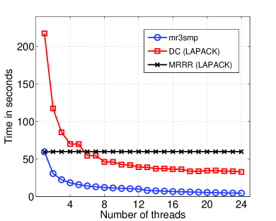
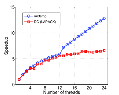
While DC takes advantage of parallelism by using a multi-threaded BLAS library, the other LAPACK routines do not exploit multi-core architectures. Once enough hardware parallelism is available, DC becomes faster than the sequential MRRR. Our parallel mr3smp on the other hand is specifically designed for multi-core processors, and results to be faster and, as Fig. 4.1 suggests, more scalable than all the other LAPACK routines. As experiments in [122] revealed, similar results hold for comparisons with the vendor-tuned Intel MKL.

4.1.2 Parallelization strategy

Existing distributed-memory versions of MRRR aim at minimizing communication among processors while attaining perfect memory balancing [13, 162]. As the division of work is performed statically, this approach comes at the expense of load balancing. Since on multi-core and shared-memory architectures the memory balance is not a concern, our objective is instead to identify the right computational granularity to distribute the workload perfectly. In this section, we illustrate how this is accomplished by dividing and scheduling the work dynamically.

The MRRR algorithm, as given in Algorithm 1, conceptually splits into two parts: (1) Computation of a root representation and initial approximation of eigenvalues; (2) Computation of eigenvectors, which includes the final refinement of eigenvalues. The two parts correspond to Lines 1–3 and 4–19 in Algorithm 1, respectively.

The first part is detailed in Algorithm 4 in Section 3.2 and is, like all the other computations, performed independently for each irreducible subblock. The computation of a root representation (as for each RRR subsequently) only costs $O(n)$ flops and is performed sequentially. The initial approximation of eigenvalues instead costs $O(n)$ flops per eigenvalue, and is performed in parallel using bisection; alternatively, whenever faster, the sequential dqds algorithm is used. Assuming a user requests $k$ eigenpairs, bisection is preferable over the dqds algorithm if the number of processors is larger than or equal to $12\cdot k/n$ [13]. In the parallel case, the computation of a subset of eigenvalues is encapsulated as an independent computational task. The granularity of the tasks ensures load balancing among the computational threads.

In the second part, we also divide the computation into tasks, which are executed by multiple threads in parallel. As many different strategies for dividing and scheduling the computation can be employed, we discuss possible variants in more detail. Although the eigenvalues are refined in the second part of the algorithm, for simplicity, we refer to the eigenvalue computation and the eigenvector computation as the first and the second part, respectively.

4.1.3 Dividing the computation into tasks

We now concentrate on the second – more costly – part of the computation. Since the representation tree, which is introduced in Section 3.1.2, characterizes the unfolding of the algorithm, it is natural to associate each node in the tree with a unit of computation. Because of this one-to-one correspondence, from now on, we use the notion of task and node interchangeably. Corresponding to interior nodes and leaf nodes, we introduce two types of tasks, C-tasks and S-tasks. C-tasks deal with the processing of clusters and create other tasks, while S-tasks are responsible for the final eigenpair computation. C-tasks and S-tasks embody the two branches of the if statement in Algorithm 1: Lines 14–17 and 10–11, respectively. The flow of the computation is schematically displayed in Fig. 4.2.

Figure 4.2: The computational flow of MRRR. An S-task performs to the final computation of eigenpairs. A C-task performs the spectrum shift, refinement, and reclassification of the eigenvalues.

Irrespective of scheduling strategies, the granularity of this first approach prevents a parallel execution of tasks: In the presence of a large cluster, the threads might run out of executable tasks well before the large cluster is processed and broken up into smaller tasks. As an example, consider the computation of the eigenpairs with indices $\{1,2,\ldots,9\}$ of an irreducible input matrix. Assume eigenvalues $\hat{\lambda}_{2}$ to $\hat{\lambda}_{9}$ are clustered, and that we want to solve the problem on a 4-core processor; in this case, one of the four cores will tackle the singleton $\{1\}$, a second core will process the cluster, and the third and forth cores will sit idle until the cluster is decomposed. Since the cluster computation is more expensive than the processing of a singleton, even the first core will have idle time, waiting for new available tasks.

Corresponding to statements 14–17 in Algorithm 1, the computation associated with a C-task is summarized in Algorithm 2.

Input: An RRR and the index set of a cluster $\mathcal{I}_{c}$, $\{\mbox{RRR},\mathcal{I}_{c}\}$.
Output: S-tasks and C-tasks associated with the children of the cluster.

1:  Call subroutine ComputeNewRRR.

2:  Call subroutine RefineEigenvalues.

3:  Call subroutine ClassifyEigenvalues.

 

Subroutine: ComputeNewRRR
Input: An RRR and the index set of a cluster $\mathcal{I}_{c}$, $\{\mbox{RRR},\mathcal{I}_{c}\}$.

1:  Compute RRR_shifted using DLARRF.

 

Subroutine: RefineEigenvalues
Input: An RRR and the index set of a cluster $\mathcal{I}_{c}$, $\{\mbox{RRR}_{shifted},\mathcal{I}_{c}\}$.

1:  if $|\mathcal{I}_{c}|>\lceil nleft/nthreads\rceil$ then

2:       Decompose the refinement into R-tasks.

3:  else

4:       Refine eigenvalues $\{\hat{\lambda}_{i}[\mbox{RRR}_{shifted}]:i\in\mathcal{I}_{c}\}$ using DLARRB.

5:  end if

 

Subroutine: ClassifyEigenvalues
Input: An RRR and the index set of a cluster $\mathcal{I}_{c}$, $\{\mbox{RRR}_{shifted},\mathcal{I}_{c}\}$.

1:  Partition $\mathcal{I}_{c}$ into subsets $\mathcal{I}_{c}=\bigcup_{s=1}^{S}\mathcal{I}_{s}$.

2:  for $s=1$ to $S$ do

3:       if $|\mathcal{I}_{s}|>1$ then

4:             Create and enqueue C-task $\{\mbox{RRR}_{shifted},\mathcal{I}_{s}\}$.

5:       else

6:             Create and enqueue S-task $\{\mbox{RRR}_{shifted},\mathcal{I}_{s}\}$.

7:       end if

8:  end for

Algorithm 2  C-task

Eigenvalues and eigenvectors are specified by their index and generally shared among all threads. Quantities $nleft$ and $nthreads$ denote the number of eigenpairs not yet computed and the number of threads used, respectively. In our implementation, an RRR is a reference counted object, which contains information such as the data of the representation, the accumulated shift, the depth in the representation tree, and a counter that indicates the number of tasks that depend on the RRR. Whenever tasks are executed that make use of an RRR, its counter is decremented; if the counter becomes zero the memory of the RRR is released. To reduce the granularity of the computation, we introduce a third type of tasks, the R-task, that allows the decomposition of the eigenvalue refinement – the most expensive step in C-tasks – originating immediately executable tasks for all threads even if large clusters are encountered. An R-task takes as input an RRR and a list of eigenvalues. As output, it returns the refined eigenvalues. As a guiding principle for load balance, we decompose C-tasks into subtasks whenever they involve more than $s_{max}=\lceil nleft/nthreads\rceil$ eigenpairs; the rationale being that at any moment, each thread is conceptually “responsible” for the computation of not more than $s_{max}$ eigenpairs. The algorithm directly invokes LAPACK’s routines DLARRF and DLARRB; we point out that if these are amended, our parallelization of MRRR still stands, without modifications.

Vice versa, to avoid too fine a granularity, we extend S-tasks to compute eigenpairs of multiple singletons from the same RRR; we call this strategy “bundling”. This form of bundling might be seen as widening the base case (by joining leaf nodes) of the recursive algorithm. Bundling brings several advantages: among them, (1) better usage of cached data through temporal and spatial locality; (2) fewer tasks and less contention for the work queues; (3) reduced false sharing; and (4) the possibility of lowering the overall memory requirement. For similar reasons, we execute C-tasks without creating additional tasks, provided they are sufficiently small.

Corresponding to Lines 10–11 in Algorithm 1, the computation performed by an S-task is summarized by Algorithm 3.

Input: An RRR and an index set $\mathcal{I}_{s}$ of well-separated eigenvalues, $\{\mbox{RRR},\mathcal{I}_{s}\}$.
Output: Local eigenpairs $\{(\hat{\lambda}_{i},\hat{z}_{i}):i\in\mathcal{I}_{s}\}$.

1:  for each index $i\in\mathcal{I}_{s}$ do

2:       while eigenpair $(\hat{\lambda}_{i},\hat{z}_{i})$ is not accepted do

3:             Invoke DLAR1V to solve $(LDL^{T}-\hat{\lambda}_{i}I)\hat{z}_{i}=N\Delta N\hat{z}_{i}=\gamma_{r}e_{r}$.

4:             Record the residual norm $|\gamma_{r}|/\|\hat{z}_{i}\|$ and the RQC $\gamma_{r}/\|\hat{z}_{i}\|^{2}$.

5:             if $|\gamma_{r}|/\|\hat{z}_{i}\|<\mbox{tol}_{1}\cdot\mbox{gap}(\hat{\lambda}_{i})$ or $|\gamma_{r}|/\|\hat{z}_{i}\|^{2}<\mbox{tol}_{2}\cdot|\hat{\lambda}_{i}|$ then

6:                  Normalize $\hat{z}_{i}$ and accept the eigenpair $(\hat{\lambda}_{i},\hat{z}_{i})$.

7:             end if

8:             if RQC improves $\hat{\lambda}_{i}$ then

9:                  $\hat{\lambda}_{i}:=\hat{\lambda}_{i}+\gamma_{r}/\|\hat{z}_{i}\|^{2}$

10:             else

11:                  Use bisection to refine $\hat{\lambda}_{i}$ to full accuracy.

12:             end if

13:       end while

14:  end for

Algorithm 3  S-task

Instead of bisection followed by one step of inverse iteration, it uses Rayleigh quotient iteration for performance reasons. The Rayleigh quotient correction (RQC) is used to improve the eigenvalue if the following applies: the sign of the correction is correct and it leads to a value within the uncertainty interval $[\hat{\lambda}_{i}-\hat{\lambda}_{i,err},\hat{\lambda}_{i}+\hat{\lambda}_{i,err}]$ [46]. When the eigenpair is accepted, a final RQC could be added to reduce the residual. For the eigenvector computation, the algorithm invokes LAPACK’s auxiliary routine DLAR1V; the same comment as for Algorithm 2 applies here. Quantities $tol_{1}=\mathcal{O}(n\varepsilon)$ and $tol_{2}=\mathcal{O}(\varepsilon)$ denote appropriate constants to signal convergence.

An example.

Figure 4.3 shows the execution trace of an exemplary eigenvector computation. The examined matrix is the one for which timings were presented in Fig. 4.1. Computing the eigenvectors took about 49.3 seconds sequentially and about 3.3 seconds with 16 threads. In the time-line graph, the green, blue and yellow sections correspond to the processing of S-tasks, C-tasks, and R-tasks, respectively. Everything considered as parallelization overhead is colored in red. On average, each thread spends about 66% of the execution time in computing the eigenvectors of singletons, 34% in computing new RRRs of clusters and to refine the associated eigenvalues. Due to the dynamic task scheduling, load balancing is achieved and almost no overhead computations occurs.

Figure 4.3: Exemplary execution trace for a matrix of size $12{,}387$ using 16 threads on Dunnington. The colors green, blue, and yellow represent time spent in the execution of S-tasks, C-tasks, and R-tasks, respectively.

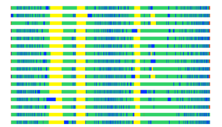
We want to point out important details of the trace. The first yellow bar corresponds to a refinement of eigenvalues that is split via R-tasks. A cluster of size $8{,}871$ is encountered by the bottommost thread. Since the cluster contains a large part of the eigenvectors that are still to be computed, the refinement of its eigenvalues is split among all the threads. The procedure of splitting the refinement among all threads is repeated two more times during the computation. Later during the computation there are yellow regions that provide examples where the refinement of eigenvalues is split into R-tasks but not distributed among all threads anymore.

4.1.4 The work queues and task scheduling

We analyze data dependencies among tasks, and discuss how they may be scheduled for execution. To differentiate the task priority, we form three work queues for high, medium, and low priority tasks, respectively. Each active thread polls the queues, from the highest to the lowest in priority, until an available task is found; the task then is dequeued and executed. The process is repeated until all eigenpairs are computed.

Task data dependencies

Since the index sets associated to C-tasks and S-tasks are disjoint, no data dependencies are introduced. Dependencies among tasks only result from the management of the RRRs. Each task in the work queues requires its parent RRR, which serves as input in Algorithms 2 and 3; as a consequence, an RRR must be available until all its children tasks are processed. A possible solution – but not the one used – is to dynamically allocate memory for each new RRR, pass the memory address to the children tasks, and keep the RRR in memory until all the children are executed. An example is given by node $\{6,7,8,9\}$ in Fig. 3.1 in Section 3.1. $M^{(2)}$ must be available as long as the children nodes $\{6,7\}$, $\{8\}$, and $\{9\}$ have not been processed. This solution offers the following advantages: When multiple threads are executing the children of a C-task, only one copy of the parent RRR resides in memory and is shared among all threads; similarly, the auxiliary quantities $d\ell(i)=D(i,i)\cdot L(i+1,i)$ and $d\ell\ell(i)=D(i,i)\cdot L(i+1,i)^{2}$, for all $1\leq i\leq n-1$, might be evaluated once and shared; in architectures with shared caches, additional performance improvements might arise from reuse of cached data. On the downside, this approach needs an extra $\mathcal{O}(n^{2})$ workspace in the worst case.

In order to reduce the memory requirement, we make the following observation. Each task can associate the portion of eigenvector matrix $Z$ corresponding to $\mathcal{I}_{c}$ in Algorithm 2 or $\mathcal{I}_{s}$ in Algorithm 3 with local workspace, i.e., a section of memory not accessed by any other task in the work queues. Continuing with the example of node $\{6,7,8,9\}$ at depth one of the tree in Fig. 3.1, the columns 6 to 9 are regarded as local storage of the corresponding task. If the RRR required as input is stored in the task’s local workspace, then we call such a task independent. If all the children of a task are independent, then the task’s RRR is not needed anymore and can be discarded. Additionally, all the children tasks can be executed in any order, without any data dependency. We now illustrate that all the C-tasks can be made independent and that practically all S-tasks can be made independent too.

C-tasks: As a cluster consists of at least two eigenvalues, the corresponding portion of $Z$ – used as local workspace – is always large enough to contain a representation. We therefore use $Z$ to store the parent RRR’s data. Unfortunately, rendering the tasks independent comes with an overhead due to storing the parent RRR into $Z$ and retrieving the parent RRR from $Z$.

S-tasks: The same approach is feasible for S-tasks whenever at least two singletons are bundled. Conversely, the approach cannot be applied in the extreme scenario in which a cluster is decomposed into smaller clusters plus only one singleton. The leaf node $\{2\}$ in Fig. 3.1 represents such an exception. All the other S-tasks may be bundled in groups of two or more, and therefore can be made independent. One drawback of this approach is that when several S-tasks children of the same node are processed simultaneously, multiple copies of the same RRR reside in memory, preventing the reuse of cached data. In the example of node $\{6,7,8,9\}$ in Fig. 3.1, storing $M^{(2)}$ into columns 6 and 7, as well as columns 8 and 9, creates an independent C-task for the node $\{6,7\}$, and an independent S-task $\{8,9\}$ in which the two singletons $\{8\}$ and $\{9\}$ are bundled. We point out that while working with independent tasks introduces some overhead, it brings great flexibility in the scheduling, as tasks can now be scheduled in any order.

Task scheduling

Many strategies can be employed for the dynamic scheduling of tasks. As a general guideline, in a shared memory environment, having enough tasks to feed all the computational cores is paramount to achieve high-performance. In this section, we discuss the implementation of two simple but effective strategies that balance task-granularity, memory requirement, and creation of tasks. In both cases, we implemented three separate FIFO queues, to avoid contention when many worker threads are used. Both approaches schedule R-tasks with high priority, because they arise as part of the decomposition of large clusters, and originate work in the form of tasks.

C-tasks before S-tasks: All enqueued C-tasks and S-tasks are made independent. (In the rare event that a S-task cannot be made independent, the task is executed immediately without being enqueued.) Consequently, all C-tasks and S-tasks in the work queues can be scheduled in any order. Since processing C-tasks creates new tasks that can be executed in parallel, we impose that C-tasks (medium priority) are dequeued before S-tasks (low priority). This ordering is a special case of many different strategies in which the execution of C-tasks and S-tasks are interleaved. No other ordering offers more executable tasks in the work queues; thus, for the scenario that all tasks are independent, we expect that the strategy attains the best performance.

S-tasks before C-tasks: No S-task is made independent. In order to obtain a similar memory requirement as in the first approach, we are forced to schedule the S-tasks before the C-tasks. The reason is that for each cluster an RRR must be kept in memory until all its children S-tasks are executed. The ordering guarantees that at any time only S-tasks originating no more than $nthreads$ clusters are in the queue, and we limit the number of RRRs to be kept in memory to $nthreads$. While the flexibility in scheduling tasks is reduced, the overhead from making the S-tasks independent is avoided. In practice, this second approach is slightly faster – about 5–8% in our tests; it is used for all timings in Section 4.1.6.

4.1.5 Memory requirement

Routines mr3smp and LAPACK’s DSTEMR make efficient use of memory by using the eigenvector matrix $Z$ as temporary storage. Additionally, DSTEMR overwrites the input matrix $T$ to store only the RRR of the currently processed node. This approach is not feasible in a parallel setting, as the simultaneous processing of multiple nodes requires storing the associated RRRs separately. Moreover, in our multi-threaded implementation, each thread requires its own workspace. As a consequence, the parallelization and its resulting performance gain come at the cost of a slightly higher memory requirement than in the sequential case.

While DSTEMR requires extra workspace to hold $18n$ double precision numbers and $10n$ integers [46], mr3smp requires extra storage of about $(12n+6n\cdot nthreads)$ double precision numbers and $(10n+5n\cdot nthreads)$ integers. For a single thread the total workspace requirement is roughly the same as for DSTEMR, and the requirement increases linearly with the number of threads participating in the computation. We remark that thanks to shared data, the required memory is less than $nthreads$ times the memory needed for the sequential routine.

(a) Using a fixed number of 12 threads.

(b) Using a fixed matrix size of $5{,}000$.

Figure 4.4: Peak memory requirement of mr3smp. The workspace requirement has to be compared with the $n^{2}$ double precision numbers of the output matrix. For instance, for matrices of size 5,000 the output requires about 190 MB memory.

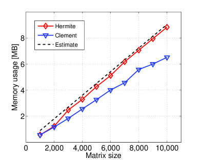
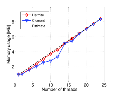
In Fig. 4.4 we show for two different kind of matrices, namely the so called Hermite and symmetrized Clement matrices, the measured peak memory usage by mr3smp. By setting $nthreads$ to 12, Fig. 4.4(a) shows that the extra memory requirement is linear in the matrix size. In Fig. 4.4(b), the matrix size has a fixed value of $5{,}000$ and the dependence of the required memory with the number of threads is shown. Although the memory requirement increases with the number of threads, even if 24 threads are used, the required extra storage only makes up for less than 5% of the memory required by the output matrix $Z$. Since the DC algorithm requires $\mathcal{O}(n^{2})$ double precision workspace, the advantage of MRRR in requiring much less memory than DC is maintained.

4.1.6 Experimental results

We now turn the attention on timing and accuracy results of mr3smp. We used similar settings for thresholds, convergence parameters, and classification criteria as DSTEMR to clearly identify the effects of the parallel execution.

We compare our solver to the fastest solvers available in LAPACK and the parallel ParEig (a solver for a distributed-memory systems). As not all solvers allow for the computation of a subset of eigenpairs at reduced cost, we consider this scenario for mr3smp first. All tests were run on Dunnington, with the settings described in Appendix C. We used LAPACK version $3.2.2$ in conjunction with Intel’s MKL BLAS version 10.2, and ParEig version $2.0$ together with OpenMPI version $1.4.2$. Descriptions of the LAPACK routines and test matrices are found in Appendix A and D, respectively. We also refer to [122, 123] for further results and additional information on the experiments.

Subset Computations

An important feature of MRRR is the ability of computing a subset of eigenpairs at reduced cost. We show that with our task-based parallelization, the same is true also in the multi-threaded case. In Fig. 4.5(a), we show mr3smp’s total execution time against the fraction of requested eigenpairs. The test matrices are of size 10,001, and the computed subsets are on the left end of the spectrum. Additionally, Fig. 4.5(b) shows the obtained speedup with respect to DSTEMR. Intuitively, the speedup is limited if very few eigenpairs are computed. However, it is often higher for computing subsets than for finding all eigenpairs.

The experiments indicate that mr3smp is especially well suited for subsets computation. However, in order to compare timings with other solvers that cannot compute subsets of eigenpairs at reduced cost, we show results for computing all eigenpairs subsequently. It is important to notice that the execution time of MRRR is proportional to the number of eigenpairs, which is not true for other methods. This makes MRRR the method of choice for computing subsets of eigenpairs, but often MRRR is the fastest method even when all eigenpairs are desired [37, 124, 13].

(a) Execution time.

(b) Speedup with respect to DSTEMR.

Figure 4.5: Computation of a subset of eigenpairs using mr3smp with 24 threads on Dunnington.

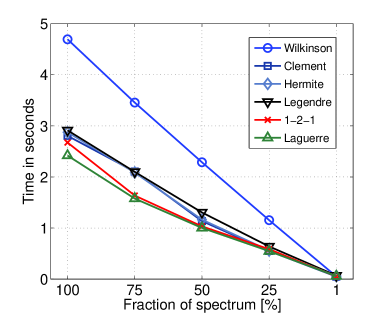
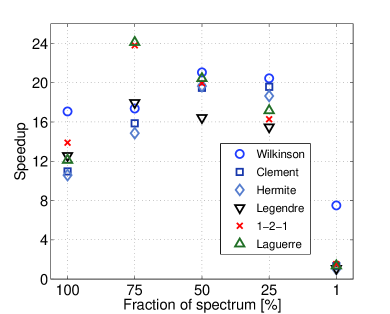
As a final note: if MRRR is used to compute small subsets of eigenpairs of dense matrices after a reduction to tridiagonal form, it might be advantageous to use successive band reduction (SBR) instead of the direct reduction to tridiagonal form provided by LAPACK. Routines for SBR are found in the SBR toolbox [19], and in vendor-tuned libraries such as Intel’s MKL.

MR³​–SMP vs. LAPACK

Arguably, the most important test matrices come from applications. In the following, we concentrate on timing and accuracy results for a set of tridiagonal matrices arising in different scientific and engineering disciplines.

In Table 4.1 we show timings for QR (DSTEQR), BI (DSTEVX), MRRR (DSTEMR), as well as for DC (DSTEDC) and MR³-SMP (mr3smp). Since they cannot achieve parallelism through multi-threaded BLAS, the execution time for the first three routines is independent of the number of threads. Conversely, both DC and mr3smp take advantage of multiple threads, through multi-threaded BLAS and the task-based approach, respectively. All the timings refer to the execution with 24 threads, that is, as many threads as cores available. The execution times for QR and BI are significantly higher than for the other algorithms; thus, we omit the results for the largest matrices. In all cases, even if parallelized and achieving perfect speedup, the routines would still be noticeably slower than the other methods. In all tests, MR³-SMP outperforms the other solvers considerably.

Matrix	Size	QR	BI	MRRR	DC	MR3–SMP
ZSM-5	$2{,}053$	$68.4$	$6.24$	$0.92$	$0.70$	0.15
Juel-k2b	$4{,}289$	$921$	$382$	$4.41$	$3.39$	0.52
Auto-a	$7{,}923$	$6{,}014$	$2{,}286$	$18.8$	$12.2$	1.88
Auto-b	$12{,}387$	$22{,}434$	$7{,}137$	$59.5$	$32.9$	4.65
Auto-c	$13{,}786$	–	$9{,}474$	$56.6$	$35.4$	5.34
Auto-d	$16{,}023$	–	–	$87.8$	$45.8$	7.76

Table 4.1: Execution times in seconds for a set of application matrices.

Fig. 4.6(a) shows mr3smp’s and DSTEDC’s (in light gray) total speedup. All the other routines do not attain any speedups at all. Regarding mr3smp, every line up to 12 threads converges to a constant value, a phenomenon which is better understood by looking at Fig. 4.6(b). For matrix Auto-b, we plot the execution time for the initial eigenvalue approximations and the eigenvectors computation separately. When all the eigenpairs are requested, the sequential dqds algorithm is used in a single-threaded execution to approximate the eigenvalues. Because of the sequential nature of the dqds algorithm, by Amdahl’s law, the maximal speedup of mr3smp is limited to about 7.6. When enough parallelism is available, bisection becomes faster than dqds; according to the criterion discussed in Section 4.1.2, if more than 12 threads are used, we switch to bisection. Such a strategy is essential to achieve scalability: using 24 threads, the speedup is about 13, that is almost twice of the limit dictated by Amdahl’s law. Moreover, all the speedup curves in Fig. 4.6(a) have positive slope at 24 threads, thus indicating that further speedups should be expected as the amount of available cores increases.

(a) Speedup.

(b) Execution time.

Figure 4.6: Speedup for the total execution time of mr3smp and DSTEDC. (a) mr3smp’s speedup is with respect to DSTEMR, while speedups for DSTEDC (shown in light gray) are with respect to its sequential execution. (b) For input matrix Auto-b, separate execution time for the initial eigenvalue approximation and for the subsequent eigenvector computation.

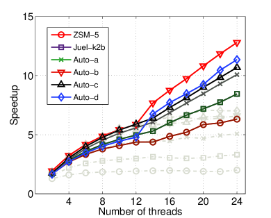
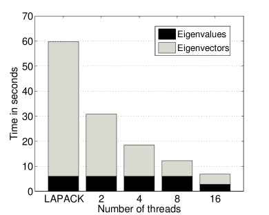
MR³​–SMP vs. ParEig

In Table 4.2 we compare the timings of mr3smp and ParEig. ParEig is designed for distributed-memory architectures, and uses the Message-Passing-Interface (MPI) for communication. Since ParEig was at the time of writing the fastest distributed-memory parallel symmetric tridiagonal eigensolver, we omit a comparison to other routines such as ScaLAPACK’s PDSTEDC. Instead, we refer to [13, 162] for comparisons of ParEig to other eigensolvers. In the experiments, we present ParEig’s timings for 22 processes as they were consistently faster than the execution with 24 processes. Timings of ParEig do not include the overhead of initializing the MPI library.

Matrix	Size	MR3-SMP	ParEig
ZSM-5	$2{,}053$	$0.15$  $(0.16)$	$0.13$
Juel-k2b	$4{,}289$	$0.52$  $(0.49)$	$1.29$
Auto-a	$7{,}923$	$1.88$  $(1.62)$	$2.89$
Auto-b	$12{,}387$	$4.65$  $(3.93)$	$5.48$
Auto-c	$13{,}786$	$5.34$  $(3.02)$	$5.98$
Auto-d	$16{,}023$	$7.76$  $(5.69)$	$7.99$

Table 4.2: Execution times in seconds for a set of matrices arising in applications. The timings in brackets are achieved if mr3smp uses the same splitting criterion as ParEig.

The performance of mr3smp matches and even surpasses that of ParEig. For a direct comparison of mr3smp with ParEig, it is important to stress that, even though both routines implement the MRRR algorithm, several internal parameters are different. Most importantly, the minimum relative gap, $gaptol$, which determines when an eigenvalue is to be considered well-separated, is set to $\min\{10^{-2},n^{-1}\}$ and $10^{-3}$ in ParEig and mr3smp, respectively. In order to make a fair comparison, in brackets we show the execution time of mr3smp when using the parameter $gaptol$ as set in ParEig. The numbers indicate that with similar tolerances, in the shared-memory environment, mr3smp outperforms ParEig.

MR³​–SMP’s accuracy

In Fig. 4.7, we present accuracy results for mr3smp and ParEig, as well as LAPACK’s DSTEMR and DSTEDC.

(a) Largest residual norm.

(b) Orthogonality.

Figure 4.7: Accuracy of mr3smp, LAPACK’s DSTEMR and DSTEDC, and ParEig for a set of application matrices. The largest residual norm and the orthogonality are defined in (2.5).

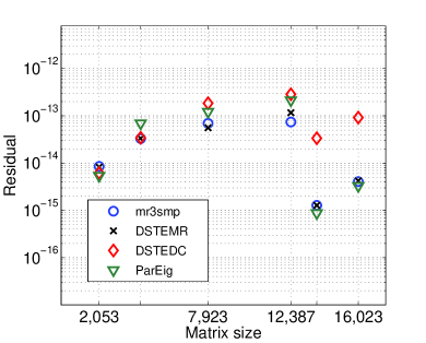
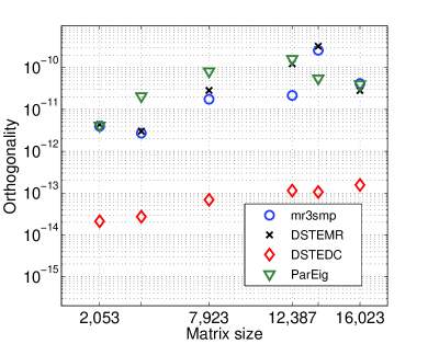
For all test matrices, the routines attain equally good residuals, while in terms of orthogonality DC is more accurate than the three MRRR-based routines. The results are underpinned by the tests of Demmel et al. [37], which shows a similar behavior for a large test set of artificial and application test matrices. In general, our parallel MRRR obtains the same accuracy as its sequential counterpart.

While the accuracy of MRRR is sufficient for many users, it might be a concern to others. It is therefore natural to ask whether the accuracy of the MRRR-based routines can be improved to levels of DC. Unfortunately, this is not an easy task as Theorem 3.1.4 shows that one needs to be prepared of orthogonality levels of about $\mathcal{O}(1000n\varepsilon)$ even if all requirements of the algorithm are fulfilled. Our workaround to this dilemma resorts to the use of higher precision arithmetic and is the topic of Chapter 5.

4.2 MRRR for modern supercomputers

In this section we present a tridiagonal solver, PMRRR, which merges the task-based approach introduced in the previous section and the distributed-memory parallelization of Bientinesi et al. [13]. Our target architecture are supercomputers with hybrid shared/distributed-memory. For these architectures, parallelism is achieved by executing multiple processes that communicate via message passing. Each of these processes in turn might execute multiple threads that communicate via shared memory. In this way, PMRRR is well-suited for both single node and large-scale massively parallel computations.

PMRRR was integrated to the Elemental library [128] for the solution of large-scale standard and generalized dense Hermitian eigenproblems (in short, GHEP and HEP, respectively). In Section 4.2.2, we introduce EleMRRR (from Elemental and PMRRR), a set of distributed-memory MRRR-based eigensolvers within Elemental. EleMRRR provides full support for hybrid message-passing and multi-threading parallelism. If multi-threading is not desired, EleMRRR can be used in purely message-passing mode.

A thorough performance study comparing EleMRRR with ScaLAPACK’s eigensolvers on two high-end computing platforms is provided. This study accomplishes two objectives: First, it reveals that the commonly used ScaLAPACK routines (PxHEGVX, PxSYGVX, PxHEEVD, PxSYEVD) present performance penalties that are avoided by calling a different sequence of subroutines and by choosing suitable settings. Second, it indicates that EleMRRR is scalable – both strongly and weakly – to a large number of processors, and outperforms the ScaLAPACK solvers even when used according to our guidelines.

4.2.1 PMRRR and its parallelization strategy

PMRRR is built on top of the multi-threaded mr3smp introduced in the previous section. Our parallelization strategy consists of two layers, a global and a local one. At the global level, the $k$ desired eigenpairs are statically divided into equal parts and assigned to the processes. Since the unfolding of the algorithm depends on the spectrum, it is still possible that the workload is not perfectly balanced among the processes; this deficit is accepted in order to achieve the more important memory balancing. At the local level (within each process), the computation is decomposed into tasks, which are equal to the ones introduced in Section 4.1. The tasks can be executed in parallel by multiple threads and lead to the dynamic generation of new tasks. The new feature is that some tasks involve explicit communication with other processes via messages.

When executed with $p$ processes, the algorithm starts by broadcasting the input matrix and by redundantly computing the root representation $M_{root}$. Once this is available, the computation of the approximations $\hat{\lambda}_{i}[M_{root}]$ via bisection is embarrassingly parallel: Each process is responsible for at most $k_{pp}=\lceil k/p\rceil$ eigenvalues. Within a process however, to obtain workload balance, the assignment of eigenvalues to threads is done dynamically.

Once the eigenvalues are computed locally, each process gathers all eigenvalues, and the corresponding eigenpairs are assigned as desired. At this point, each process redundantly classifies the eigenvalues into singletons and clusters and only enqueues tasks that involve eigenpairs assigned to the process. To increase workload balance, the first classification of eigenvalues is amended with a criterion based on the absolute gaps of the eigenvalues [161, 162, 163].

Locally, the calculation of the eigenpairs is split into computational tasks of three types as in MR³-SMP: S-tasks, C-tasks, and R-tasks. Multi-threading support within each process is easily obtained by having multiple threads dequeue and execute tasks. In contrast to the multi-core parallelization, the C-tasks must deal with two scenarios: ($i$) no communication is required to process the task, or ($ii$) communication with other processes is required for its execution. The computation associated with each of the three tasks is detailed below.

1. S-task: The corresponding eigenpairs are computed locally as in Algorithm 3. No further communication among processes is necessary.

2. C-task: When a cluster contains eigenvalues assigned to only one process, no cooperation among processes is needed. The necessary steps are the same as those in Algorithm 2. When a cluster contains a set of eigenvalues which spans multiple processes, inter-process communication is needed. In this case, all involved processes redundantly compute a new RRR, the local set of eigenvalues is refined, and the eigenvalues of the cluster are communicated among the processes. At this point, the eigenvalues of the cluster are reclassified and the corresponding tasks created and enqueued.

3. R-task: Exactly as in MR³-SMP, the task is used to split the work for refining a set of eigenvalue among threads.

In order to deal with the two different flavors of C-tasks, Algorithm 2 is modified: for each C-task it checks whether communication with other processes is required. If communication is required, the refinement is limited to the portion of eigenvalues assigned to the process and a communication of refined eigenvalues among the involved processes is added. If no communication is required, the task corresponds to Algorithm 2.

While the overall execution time depends on the spectral distribution, the memory requirement is matrix independent (with $\mathcal{O}(nk/p)$ floating point numbers per process), and perfect memory balance is achieved [13, 162]. To appreciate this feature, we mention that such a memory balance is not guaranteed by ScaLAPACK’s bisection and inverse iteration implementation. In this case, clusters are processed within a single process, effectively leading (in the worst case) to a requirement of $\mathcal{O}(nk^{2})$ operations and $\mathcal{O}(nk)$ floating point numbers memory for a single process.

Our tests show that the hybrid parallelization approach is equally fast than the one purely based on MPI. This is generally true for architectures with a high degree of inter-node parallelism and limited intra-node parallelism. By contrast, on architectures with a small degree of inter-node parallelism and high degree of intra-node parallelism, we expect the hybrid execution of PMRRR to be preferable to pure MPI.

We stress that even when no multi-threading is used, the task-based design of PMRRR is advantageous: By scheduling tasks that require inter-process communication with priority and using non-blocking communication, processes continue executing tasks while waiting to receive data. This strategy often leads to a perfect overlap of communication and computation. As an example, the scalability advantage of PMRRR compared with ScaLAPACK’s PDSTEMR in Fig. 4.10(b) is the result of non-blocking communications; in the experiment with $1{,}024$ cores, ScaLAPACK’s MRRR spends about 30 out of 50 seconds in exposed communication.

4.2.2 Elemental’s eigensolvers

Elemental’s eigensolvers, HermitianGenDefiniteEig and HermitianEig, follow the classical reduction and backtransformation approach described in Sections 2.3.2 and 2.3.3. As Elemental’s solvers are equivalent to their sequential counterparts in terms of accuracy, we concentrate on their performance in later experiments. In terms of memory, Elemental’s solvers are quite efficient. In Table 4.3, we report approximate total memory requirements for computing $k$ eigenpairs of generalized and standard eigenproblems. As a reference, we provide the same numbers for the solvers we later built from ScaLAPACK routines. (In Section 4.2.4, we define the meaning of “ScaLAPACK DC” and “ScaLAPACK MRRR” precisely.) The numbers in the table are expressed in units of the size of a single complex and real floating point number, depending on the required arithmetic. The memory requirement per process can be obtained by dividing by the total number of processes.

	Complex		Real
	GHEP	HEP	GHEP	HEP
ScaLAPACK DC	$4n^{2}$	$3n^{2}$	$5n^{2}$	$4n^{2}$
ScaLAPACK MRRR	$2n^{2}+1.5nk$	$n^{2}+1.5nk$	$2n^{2}+2nk$	$n^{2}+2nk$
Elemental	$2n^{2}+nk$	$n^{2}+nk$	$2n^{2}+nk$	$n^{2}+nk$

Table 4.3: Total memory requirements in units of complex and real floating point numbers for the computation of $k$ eigenpairs.

For performance reasons, as we discuss later, both Elemental and ScaLAPACK are best executed with processes that are logically organized in a two-dimensional grid. For square process grids, Elemental’s memory requirement is between $0.5n^{2}$ and $2n^{2}$ floating point numbers lower than that of the ScaLAPACK-based solvers. If non-square grids are used, a user concerned about memory usage can make use of the non-square reduction routines – at the cost of suboptimal performance. The reduction routines for square process grids would otherwise need a data redistribution that adds a $n^{2}$ term to Elemental and ScaLAPACK MRRR, but not to DC. However, in this situation, ScaLAPACK MRRR can save workspace to perform its redistribution of the eigenvectors from a one-dimensional to a two-dimensional block-cyclic data layout, reducing its terms by $nk$ real floating point numbers. This eigenvector redistribution is performed in Elemental in-place, resulting in a smaller memory footprint than possible for ScaLAPACK’s routines.

Subsequently, we call Elemental’s eigensolvers based on PMRRR briefly EleMRRR. Before we show experimental results of EleMRRR, we make a little detour discussing ScaLAPACK’s solvers. The reason being that the solvers that are included in the library each present performance penalties, which are easily avoided. In order to have a fair comparison, and to provide our findings to a large group of ScaLAPACK users, we build eigensolvers from a sequences of ScaLAPACK routines with optimal settings, which are generally faster than the commonly used solvers.

4.2.3 A study of ScaLAPACK’s eigensolvers

Highly parallel computers (e.g., Juropa, which is used for the experiments below and described in Appendix C) are frequently used when the execution time and/or the memory requirement of a simulation become limiting factors. With respect to execution time, the use of more processors would ideally result in faster solutions. When memory is the limiting factor, additional resources from large distributed-memory environments should enable the solution of larger problems. We study the performance of eigensolvers for both situations: increasing the number of processors while keeping the problem size constant (strong scaling), and increasing the number of processors while keeping the memory per processors constant (weak scaling).

ScaLAPACK is a widely used library for the solution of large-scale dense eigenproblems on distributed-memory systems. Version 1.8 of the library, at the time of performing the experiments the latest release, is used within this section. Later versions, such as 2.0 (released in Nov. 2011), presents no significant changes in the tested routines. From version 2.0 on, the MRRR-based routines for the HEP are added to the library. The available routines for the GHEP and HEP and their functionality are described in Appendix A. Without loss of generality, we concentrate on the case of double precision complex-valued input.

Generalized eigenproblems

As presented in Table A.5 of Appendix A, PZHEGVX is ScaLAPACK’s only routine for Hermitian generalized eigenproblems. The routine implements the six-stage procedure described in Section 2.3.3 and is based on bisection and inverse iteration. In Fig. 4.8(a), we report the weak scalability of PZHEGVX for computing 15% of the eigenpairs of $Ax=\lambda Bx$ associated with the smallest eigenvalues. This task frequently arises in electronic structure calculations via density functional theory (DFT); some methods require between 1/6 and 1/3 of the eigenpairs associated with the smallest eigenvalues of a large number matrices whose dimensions can be in the tens of thousands [141]. Fig. 4.8(a) indicates that as the problem size and the number of processors increase, PZHEGVX does not scale as well as EleMRRR, which we included as a reference.

(a) Execution time.

(b) Breakdown of time by stages.

Figure 4.8: Weak scalability for the computation of 15% of the eigenpairs. As commonly done in practice, the eigenvectors are requested to be numerically orthogonal [148].

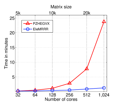
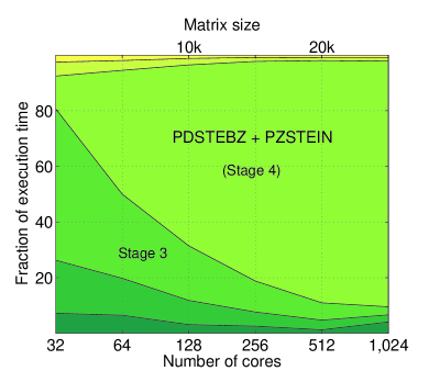
By Fig. 4.8(b), it is evident that the routines PDSTEBZ and PZSTEIN, which implement BI for the tridiagonal stage, are the main cause for the poor performance of PZHEGVX. For instance in the problem of size $20{,}000$, these routines are responsible for almost 90% of the compute time. BI’s poor performance is a well-understood phenomenon (e.g., see the comments in [26] and Section 2.3), directly related to the effort necessary to orthogonalize eigenvectors corresponding to clustered eigenvalues. This issue led to the development of MRRR, which avoids the orthogonalization entirely. In addition to the performance issue, PZHEGVX suffers from memory imbalances, as all the eigenvalues belonging to a cluster are computed on a single processor.

Observation 1.

In light of the above considerations, the use of ScaLAPACK’s routines based on bisection and inverse iteration is not recommended.

Consequently, we do not provide further comparisons between EleMRRR and PZHEGVX or PDSYGVX. Instead, we illustrate how the performance of these drivers changes when BI for the tridiagonal eigensolver is replaced with other – faster – methods, namely DC and MRRR.

Standard eigenproblems

Among the solvers available in ScaLAPACK, only PZHEEVX (BI) and PZHEEVR (MRRR) offer the possibility of computing a subset of eigenpairs. PZHEEVX is widely used, even though, as highlighted in the previous section, it is highly non-scalable. Similarly, if eigenvectors are computed, the QR algorithm is known to be slower than DC for large problems [13]. Therefore, we omit comparisons with routines that are based on the QR algorithm. However, as discussed Section 2.3.2, QR requires significantly less memory than DC.

Observation 2.

Provided enough memory is available, ScaLAPACK’s DC is preferable over QR.

We now focus on the weak scalability of PZHEEVD, which uses DC for the tridiagonal eigenproblem. For an experiment similar to that of Fig. 4.8, we show the results for PZHEEVD and EleMRRR in Fig. 4.9(a).

(a) Execution time.

(b) Execution time of the first stage.

Figure 4.9: Weak scalability for the computation of all eigenpairs using DC. (a) Total execution time of PZHEEVD and EleMRRR. (b) Execution time for ScaLAPACK’s routines PZHETRD and PZHENTRD, which are responsible for the reduction to tridiagonal form. The former, used within the routine PZHEEVD, causes a performance penalty and accounts for much of the time difference compared with EleMRRR.

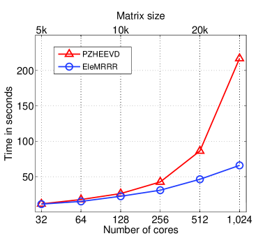
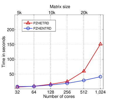
Note that all eigenpairs were computed, since PZHEEVD does not allow for subset computation. While BI might dominate the run time of the entire eigenproblem, DC required less than 10% of the total execution time. Instead, as the matrix size increases, the reduction to tridiagonal form (PZHETRD) becomes the performance bottleneck, requiring up to 70% of the total time. A comparison of Fig. 4.9(a) and Fig. 4.9(b) reveals that, for large problems, using PZHETRD for the reduction to tridiagonal form is more time consuming than the complete solution with EleMRRR.

ScaLAPACK also includes PZHENTRD, a routine for the reduction to tridiagonal form especially optimized for square processor grids. The performance improvement with respect to PZHETRD can be so dramatic that, for this stage, it is preferable to limit the computation to a square number of processors and redistribute the matrix accordingly [72]. Provided enough workspace is made available, a necessary redistribution is automatically done within PZHENTRD. In any case, it is important to note that the performance benefit of PZHENTRD is only exploited if the lower triangle of the input matrix is stored, otherwise the slower routine, PZHETRD, is invoked.

Observation 3.

ScaLAPACK’s reduction routines optimized for square grids of processors are to be preferred over the regular reduction routines, even when non-square process grids are used; moreover, only the lower triangle of implicitly Hermitian matrices should be referenced.

For performance and scalability reasons, we use the reduction routines that are optimized for square grids to build the fastest solver within the ScaLAPACK framework.

Tridiagonal eigenproblems

In contrast to all other stages of generalized and standard eigenproblems, the number of arithmetic operations of the tridiagonal eigensolver depends on the input data. When all eigenpairs are desired, depending on the matrix entries, either DC or MRRR may be faster. Fig. 4.10 provides an example of how performance is influenced by the input data.

(a) 1–2–1 type.

(b) Wilkinson type.

Figure 4.10: Weak scalability for the computation of all eigenpairs of two different test matrix types. The left and right graphs have different scales. The execution time of the MRRR routines should remain roughly constant as the number of cores is increased. In contrast to the results reported in [162], where a similar experiment to comparing PDSTEDC and PDSTEMR is performed, even when the matrices offer an opportunity for heavy deflation, eventually our PMRRR becomes faster than DC due to its superior scalability.

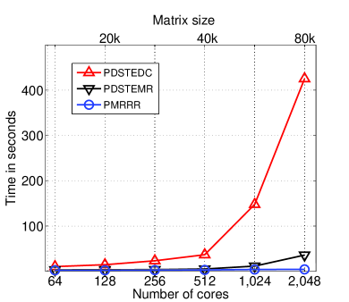
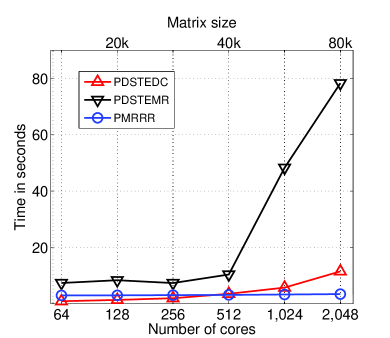
We already justified why we only consider DC and MRRR in our experiments. DC is implemented as PDSTEDC [151]. The MRRR routine corresponds to the tridiagonal stage of PDSYEVR [162] and it is not available as a separate routine; nonetheless, we call it PDSTEMR subsequently. Both routines are compared on two types of test matrices: “1–2–1” and “Wilkinson”. Due to deflation, the Wilkinson matrices are known to strongly favor the DC [104]. For both matrix types, the ScaLAPACK codes do not scale to a large number of cores and PMRRR eventually becomes the fastest solver.

Observation 4.

ScaLAPACK’s tridiagonal eigensolvers based on DC and MRRR are generally fast and reasonably scalable; depending on the target architecture and specific requirements from the application, either one may be used. Specifically, if only a small subset of the spectrum has to be computed, in terms of performance, the MRRR-based solver is to be preferred to DC. In terms of accuracy, DC is to be preferred.

Later, we include experimental data on generalized eigenproblems for both DC and MRRR. One of the challenges in building a scalable solver is that every stage must be scalable. This is illustrated in Fig. 4.11, which shows the results for ScaLAPACK’s DC for a GHEP of size $20{,}000$. While the reduction to tridiagonal form and the tridiagonal eigensolver are respectively the most and the least expensive stages on $64$ cores, on $2{,}048$ cores the situation is reversed. The behavior is explained by the parallel efficiencies shown in Fig. 4.11(b).

(a) Breakdown of time by stages.

(b) Parallel efficiency as in (2.8).

Figure 4.11: Scalability of the computation of all eigenpairs for a GHEP of size 20,000 using ScaLAPACK’s DC. The details of the experiment can be found in [124].

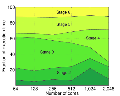
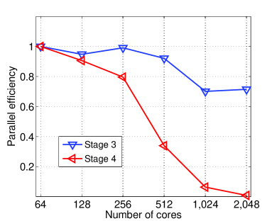
The ScaLAPACK experiments demonstrate that a comparison with the commonly used routines would be misleading. In fact, by calling the suitable set of routines, we can build much faster solvers within the ScaLAPACK framework. We use these fast solvers to compare EleMRRR with. However, we stress that what we call “ScaLAPACK’s DC” and “ScaLAPACK’s MRRR” do not correspond to routines in ScaLAPACK and are not (yet) frequently used in practice.

4.2.4 Experimental results

We present experimental results for the execution on two state-of-art supercomputers at the Research Center Jülich, Germany: Juropa and Jugene. In this section we concentrate on Juropa; results on Jugene are similar and outsourced to Appendix E. We limit ourselves to generalized eigenproblems of the form $Ax=\lambda Bx$; the results for standard eigenproblems are given implicitly by stages three to five.

All tested routines were compiled using the Intel compilers (ver. 11.1) with the flag -O3 and linked to the ParTec’s ParaStation MPI library (ver. 5.0.23). Generally, we used a two-dimensional process grid $P_{r}\times P_{c}$ (number of rows $\times$ number of columns) with $P_{r}=P_{c}$ whenever possible, and $P_{c}=2P_{r}$ otherwise. If not stated otherwise, one process per core was employed.

The ScaLAPACK library (ver. 1.8) was used in conjunction with Intel’s MKL BLAS (ver. 10.2). From extensive testing, we identified that in all cases the optimal block size was close to 32; therefore, we carried out the ScaLAPACK experiments only with block sizes of 16, 32, 48; the best result out of this pool is then reported. Since no driver for the generalized eigenproblem that makes use of DC is available, we refer to ScaLAPACK’s DC as the following sequence of routines: PZPOTRF–PZHENGST–PZHENTRD–PDSTEDC–PZUNMTR–PZTRSM. Similarly, ScaLAPACK’s MRRR corresponds to the same sequence with PDSTEDC replaced by PDSTEMR. We do not use routines PZHEGST and PZHETRD for the reduction to standard and tridiagonal form, respectively. Instead, we replaced them (when necessary) by the faster PZHENGST and PZHENTRD. Furthermore, in order to make use the fast reduction routines, only the lower triangular part of the matrices is referenced, and enough memory for a possible redistribution of the data is provided.

Elemental (ver. 0.6) – incorporating PMRRR (ver. 0.6) – was used for the EleMRRR timings. In general, since Elemental does not tie the algorithmic block size to the distribution block size, different block sizes could be used for each of the stages. We do not exploit this fact in the reported timings. Instead the same block size is used for all stages. A block size of around 96 was optimal in all cases, therefore, experiments were carried out for block sizes of 64, 96, and 128, but only the best timings are reported.

Since the timings of the tridiagonal eigenproblem depend on the input data, so does the overall solver. In order to compare fairly different solvers, we fixed the spectral distribution: for $1\leq k\leq n$, $\lambda_{k}=2-2\cos(\pi k/(n+1))$. The performance of every other stage is data independent. Moreover, since the output of the tridiagonal solvers has to be in a format suitable for the backtransformation, the MRRR-based routines have to undergo a data redistribution; in all the experiments, the timings for Stage 4 include the cost of such a redistribution.

Strong Scaling

In Fig. 4.12(a), we present timings of EleMRRR for fixed problem of size $20{,}000$. Fig. 4.12(b) shows the parallel efficiency as defined in (2.8); the reference is the execution on 64 cores.

(a) Execution time.

(b) Parallel efficiency.

(c) Breakdown of time by stages.

(d) Parallel efficiency.

Figure 4.12: Strong scalability for the computation of all eigenpairs, $Ax=\lambda Bx$. Matrices $A$ and $B$ are of size $20{,}000$. (a) Total execution time in a log-log scale. (b) Parallel efficiency as defined in (2.8); normalized to the execution using 64 cores. (c) Fraction of time spent in all six stages of the computation. The time spent in the last three stages is proportional to the number of eigenpairs computed. (d) Parallel efficiency for all six stages of the computation.

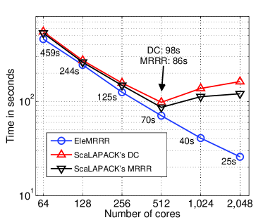
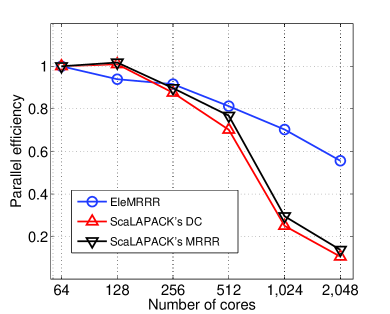
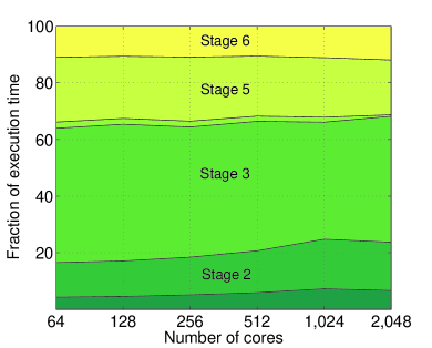
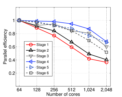
Once the proper sequence of routines is rectified, the performance of ScaLAPACK is comparable to that of EleMRRR, up to 512 cores (see Fig. 4.12). For 64 to 512 cores, ScaLAPACK’s DC is about 10% to 40% slower than EleMRRR, while ScaLAPACK’s MRRR is about 7% to 20% slower. The advantage of EleMRRR mainly comes from the Stages 1, 2, and 6, i.e., those related to the generalized eigenproblem. The timings for the standard problem (Stages 3–5) are nearly identical for all solvers, with DC slightly slower than both MRRR-based solutions.

The story for $1{,}024$ and $2{,}048$ cores changes; the performance of ScaLAPACK’s routines for the generalized eigenproblem drops dramatically. Compared to DC, EleMRRR is about 3.3 and 6.3 times faster; with respect to ScaLAPACK’s MRRR instead, EleMRRR is 2.7 and 4.7 times faster. The same holds for the standard eigenproblem, where EleMRRR is about 2.9 and 6.2 times faster than DC and 1.9 and 3.7 times faster than MRRR.

In Figs. 4.12(c) and  4.12(d), we take a closer look at the six different stages of EleMRRR. Fig. 4.12(c) tells us that roughly one third of EleMRRR’s execution time – corresponding to Stages 4, 5, and 6 – is proportional to the fraction of computed eigenpairs. Computing a small fraction of eigenpairs would therefore require about two thirds of computing the complete decomposition. In Fig. 4.12(d), we report the parallel efficiency for all six stages separately. When analyzed in conjunction with the left figure, this figure indicates if and when a routine becomes a bottleneck due to bad scaling.

The most time consuming stages are the reduction to tridiagonal form, the reduction to standard form, and the first backtransformation; the tridiagonal eigensolver (Stage 4) is negligible. Stage 4 attains the highest parallel efficiency and contributes for less than 2.2% of the overall run time.

Up to $1{,}024$ cores, ScaLAPACK’s MRRR shows a similar behavior: the tridiagonal stage makes up for less than 6% of the execution time. With $2{,}048$ cores instead, the percentage increases to 21. The situation is even more severe for DC, as the fraction spent in the tridiagonal stage increases from about 4.5% with $64$ cores to 41% with $2{,}048$ cores [Fig. 4.11(a)]. The experiment illustrates that the tridiagonal stage, unless as scalable as the other stages, will eventually account for a significant portion of the execution time.

Weak Scaling

Fig. 4.13 shows EleMRRR’s timings, when the matrix size increases (from $14{,}142$ to $80{,}000$) together with the number of cores (from $64$ to $2{,}048$). Fig. 4.13(a) contains the parallel efficiency as defined in (2.10), where the reference configuration is the same as in the previous section (the reference matrix size is $14{,}142$).

(a) Execution time.

(b) Parallel efficiency.

Figure 4.13: Weak scalability for the computation of all eigenpairs, $Ax=\lambda Bx$. Matrices $A$ and $B$ are varied in size such that the memory requirement per core remains constant.

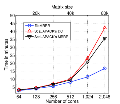
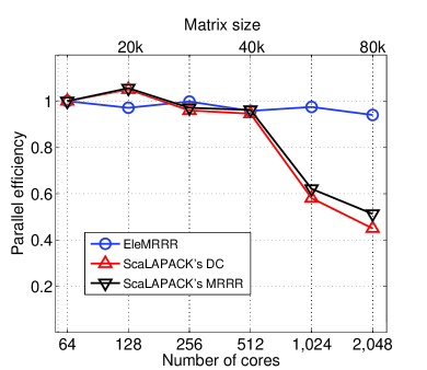
In the tests using 512 cores and less, EleMRRR outperforms ScaLAPACK only by a small margin, while using $1{,}024$ cores and more, the difference becomes significant. The right graph indicates that EleMRRR scales well to large problem sizes and high number of processes, with parallel efficiency close to one. Thanks to its better scalability, for the biggest problem, EleMRRR is 2.1 and 2.5 times faster than ScaLAPACK’s MRRR and DC, respectively.

The execution time is broken down into stages in Fig. 4.14(a).

(a) Breakdown of time by stages.

(b) Hybrid mode execution.

Figure 4.14: EleMRRR’s weak scalability for the computation of all eigenpairs. (a) Fraction of the execution time spent in the six stages, from bottom to top. (b) Comparison between a pure MPI execution and a hybrid execution using one process per socket with four threads per process.

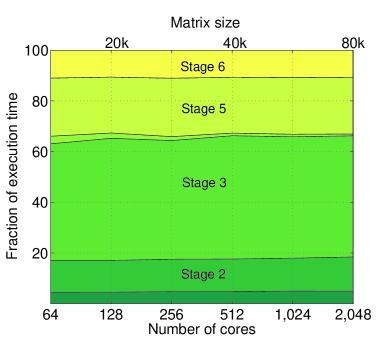
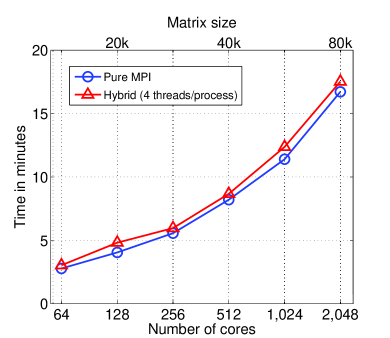
Four comments follow: (1) The time spent in PMRRR (Stage 4) is in the range of 2.5% to 0.7% and it is completely negligible, especially for large problem sizes. The timings relative to only Stage 4 are detailed in Fig. 4.10(a). (2) The timings corresponding to the standard eigenproblem (Stages 3–5) account for about 72% of the generalized problem’s execution time. (3) The part of the solver whose execution time is roughly proportional to the fraction of desired eigenpairs (Stages 4–6) makes up 32%–37% of the execution for both the GHEP and HEP. (4) No one stage in EleMRRR becomes a performance bottleneck, as all of them scale equally well.

Fig. 4.14(b) shows the execution of EleMRRR using one process per socket with four threads per process. The resulting execution time is roughly the same as for the pure MPI execution, highlighting the potential of Elemental’s hybrid mode. Further experimental results can be found in Appendix E.

4.2.5 Remaining limitations

We have shown that, in context of direct methods for generalized and standard Hermitian eigenproblems, the tridiagonal stage is often negligible. However, because of the lower complexity of MRRR, inefficiencies in the tridiagonal stage do not become visible. For PMRRR, there are three major issues remaining:

• Although mostly negligible in terms of execution time, PMRRR is the primary source of “loss of orthogonality” in the overall solution (see Section 5.3.2).

• When matrices possess large clusters of eigenvalues, the work is increased, load balance issues arise, and communication among processes is introduced. As a consequence, parallel scalability is limited (see experiments below).

• For some inputs, accuracy is not guaranteed as one or more representation is accepted without passing the test for its requirements (see Line 20 of Algorithm 8).

While the last point is discussed in the next chapter, at this point, we illustrate the remaining performance and accuracy issues of PMRRR. As the performance is matrix depended, we use a set of artificial matrices for our experiment. In Fig. 4.15, we show strong scaling results for matrices of size 20,001. The experiment corresponds to the one displayed in Fig. 4.12, but differs in two respects. First, we used a hybrid execution with one process per node and eight threads per process; the pure MPI results however are very similar. Second, while in the dense case the redistribution from one-dimensional to two-dimensional matrix layout is considered part of the tridiagonal stage, here it is excluded from the timings.

(a) Execution time.

(b) Parallel efficiency.

Figure 4.15: Strong scalability for the computation of all eigenpairs.

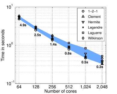
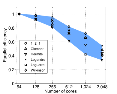
For all test matrices, the execution time of PMRRR is negligible in the dense case. For instance, EleMRRR timings for the generalized problem are 459 seconds and 25 seconds on 64 cores and 2,048 cores, respectively. Also, PMRRR’s parallel efficiency is in the same ballpark as for the other stages of the dense problem. Although timings and scalability are sufficient in context of dense problems, the parallel efficiency drops to only about 0.5 on 2,048 cores. Consequently, if we further increase the number of cores, we cannot expect an adequate reduction in run time.

In Fig. 4.16, we detail the weak scaling results of Figs. 4.10, 4.13 and 4.14. We use a hybrid execution mode, but the results for pure MPI are very similar. For 1-2-1 and Wilkinson type matrices, Fig. 4.10 shows similar results, but with a different scale.

(a) Execution time.

(b) Parallel efficiency.

Figure 4.16: Weak scalability for the computation of all eigenpairs.

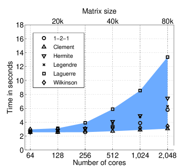
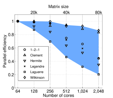
According to Figs. 4.13 and 4.14, for the largest problem of size $80{,}000$ on 2,048 cores, Elemental requires for the generalized eigenproblem about 1000 seconds and for the standard eigenproblem about 700 seconds. For all the test matrices, PMRRR contributes less than 15 seconds to the execution time; and this only if all eigenpairs are computed. However, the parallel efficiency drops dramatically for some matrices, while it behaves well for others. Ideally, the execution time would remain constant as the number of cores are increased. This is roughly observed for the Clement and Wilkinson matrices. For the Laguerre matrices however, the parallel efficiency clearly degenerates.

The loss in efficiency is directly related to the clustering of the eigenvalues. To formalize clustering, we define clustering $\rho\in[1/n,1]$ to be the largest encountered cluster divided by the matrix size. For two extreme case, we show clustering and parallel efficiency in Table 4.4. High clustering has two negative impacts: (1) The overall work is increased by $\mathcal{O}(\rho n^{2})$ flops. As clustering tends to increase for large matrices, in practice, MRRR does not quite performs work proportional to $n^{2}$ [37]; (2) The static assignment of eigenpairs to processes leads to workload imbalance.

Metric	Matrix	Matrix size
		$20{,}001$	$28{,}285$	$40{,}001$	$56{,}569$	$80{,}001$
Clustering	Wilkinson	$1.5e{-4}$	$1.1e{-4}$	$7.5e{-5}$	$5.3e{-5}$	$3.8e{-5}$
	Laguerre	$0.46$	$0.49$	$0.51$	$0.52$	$0.53$
Efficiency	Wilkinson	$0.98$	$0.96$	$0.94$	$0.91$	$0.88$
	Laguerre	$0.87$	$0.70$	$0.46$	$0.32$	$0.20$

Table 4.4: Clustering and parallel efficiency for the two extreme types of test matrices. If $\rho$ is close to $1/n$, the parallel efficiency remains good.

The available parallelism is conservatively approximated by $\rho^{-1}$. The measure is pessimistic as it assumes that clusters are processed sequentially. In reality, the bulk of the work in processing clusters is parallelized: (1) the refinement of the eigenvalues via R-tasks in the shared-memory environment and C-tasks with communication in the distributed-memory environment; (2) the final computation of the eigenpairs. However, significant clustering poses limitations on scalability, while small clustering implies great potential for parallelism.

While PMRRR’s performance is quite satisfactory for most practical purposes (especially in context of dense eigenproblems), its accuracy can be problematic. PMRRR generally obtains similar accuracy to its sequential and multi-core counterparts, which was already discussed in Section 4.1.6: For all MRRR implementations, we must be prepared for orthogonality of about $1000n\varepsilon$.

(a) Largest residual norm.

(b) Orthogonality.

Figure 4.17: Accuracy of PMRRR for the following matrices: ($\bigcirc$) 1–2–1, ($\vartriangle$) Clement, ($\triangledown$) Hermite, ($\times$) Legendre, ($\Box$) Laguerre, and ($\Diamond$) Wilkinson.

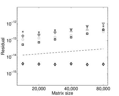
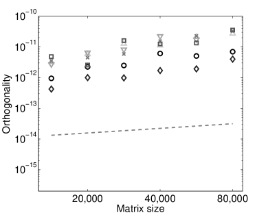
In Fig. 4.17, we show the largest residual norm and the orthogonality as defined in (2.5). Both quantities growth linearly with the matrix size. The orthogonality results are bounded by $n\varepsilon$, which is better than the worst case expected for other matrices. Nevertheless, the accuracy is not at the level of the most accurate methods, which we approximated by $\varepsilon\sqrt{n}$ (the dashed line).

Chapter 5 Mixed Precision MRRR

In the previous chapter, we showed that ($i$) MRRR is oftentimes used in context of direct methods for Hermitian eigenproblems; ($ii$) MRRR is frequently the fastest algorithm; and, ($iii$) MRRR is less accurate than other methods. In particular for dense eigenproblems, MRRR is responsible for much of the loss of orthogonality. However, it has a lower computational complexity than the reduction to tridiagonal form, which requires $\mathcal{O}(n^{3})$ arithmetic operations. These observations raise the question whether it is possible to trade (some) of MRRR’s performance to obtain better accuracy.

For any MRRR-based solver, we present how the use of mixed precisions leads to more accurate results at very little or even no extra costs in terms of performance. In this way, MRRR-based solvers are not only among of the fastest but also among the most accurate methods. An important feature of our approach is that leads to more scalable and more robust implementations.

At this point, we assume that the reader is familiar with the content of Chapter 3. In particular, Algorithm 2 and Theorem 3.1.4 serve as the basis of the following discussion.

5.1 A mixed precision approach

The technique is simple, yet powerful: Inside the algorithm, we use a precision higher than of the input/output in order to improve accuracy. To this end, we build a tridiagonal eigensolver that differentiates between two precisions: (1) the input/output precision, say binary_ x, and (2) the working precision, binary_y, with $y\geq x$. If $y=x$, we have the original situation of a solver based on one precision; in this case, the following analysis is easily adapted to situations in which we are satisfied with less accuracy than achievable by MRRR in $x$-bit arithmetic. Since we are interested in accuracy that cannot be accomplished in $x$-bit arithmetic, we restrict ourselves to the case $y>x$. Provided the unit roundoff of the $y$-bit format is sufficiently smaller than the unit roundoff of the $x$-bit format, say four or five orders of magnitude, we show how to obtain, for practical matrix sizes, improved accuracy to the desired level.

Although any $x$-bit and $y$-bit floating point format might be chosen, in practice, only those shown in Table 5.1 are used in high-performance libraries. For example, for binary32 input/output (single precision), we might use a binary64 working format (double precision). Similarly, for binary64 input/output, we might use a binary80 or binary128 working format (extended or quadruple precision). For these three configurations, we use the terms single/double, double/extended, and double/quadruple; practical issues of their implementation are discussed in Section 5.2. In this section, however, we concentrate on the generic case of binary_ x/binary_y and only use the concrete cases to illustrate our arguments.

Name	IEEE-754	Precision	Support
single	binary32	$\varepsilon_{s}=2^{-24}$	Hardware
double	binary64	$\varepsilon_{d}=2^{-53}$	Hardware
extended	binary80	$\varepsilon_{e}=2^{-64}$	Hardware
quadruple	binary128	$\varepsilon_{q}=2^{-113}$	Software

Table 5.1: The various floating point formats used and their support on common hardware. The $\varepsilon$-terms denote the unit roundoff error (for rounding to nearest). We use the letters $s$, $d$, $e$ and $q$ synonymously with 32, 64, 80, and 128. For instance, $\varepsilon_{{}_{32}}=\varepsilon_{s}$.

In principle, we could perform the entire computation in $y$-bit arithmetic and, at the end, cast the results to form the $x$-bit output; for all practical purposes, we would obtain the desired accuracy. This naive approach is not satisfactory for two reasons: First, since the eigenvectors need to be stored explicitly in the binary_y format, the memory requirement is increased; and second, if the $y$-bit floating point arithmetic is much slower than the $x$-bit one, the performance suffers severely. While the first issue is addressed rather easily (as discussed Section 5.1.2), the latter requires more care. The key insight is that it is unnecessary to compute eigenpairs with residual norms and orthogonality bounded by say $1000n\varepsilon_{y}$; instead, these bounds are relaxed to $\varepsilon_{x}\sqrt{n}$ (for example, think of $\varepsilon_{x}\approx 10^{-16}$, $\varepsilon_{y}\approx 10^{-34}$, and $n\approx 10{,}000$). While in the standard MRRR the choice of algorithmic parameters is very restricted, as we show below, we gain enormous freedom in their choice. In particular, while meeting more demanding accuracy goals, we are able to select values such that the amount of necessary computation is reduced, the robustness is increased, and parallelism is improved.

To illustrate our goal of trading performance for accuracy, we use the double/quadruple case as an example. As depicted in Fig. 5.1(b), the standard MRRR, represented by LAPACK’s DSTEMR, computes eigenpairs with accuracy achievable using double precision arithmetic; with a significant performance penalty, Fig. 5.1(a), QSTEMR, which is an adaptation of DSTEMR for quadruple precision, naturally computes more accurate results. In a naive approach, we use such a solver to achieve better accuracy and cast the result to double precision. However, all extra accuracy provided by QSTEMR is lost once the result is transformed.

(a) Relative execution time.

(b) Accuracy.

Figure 5.1: (a) Execution time of the mixed precision solver relative to the standard MRRR and a naive approach to improve accuracy. In the experiment, all eigenpairs were computed and all solvers executed sequentially. The experiment was performed on Westmere with the application matrices from Table F.1 of Appendix F. (b) Accuracy in form of orthogonality of the eigenvectors. As a reference, we added $\varepsilon_{d}$ and $\varepsilon_{q}$ as dashed lines.

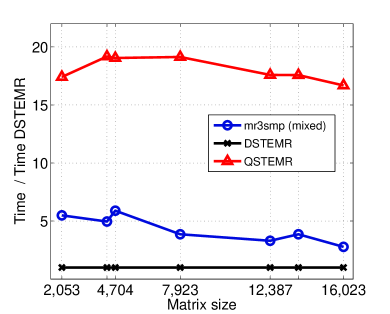
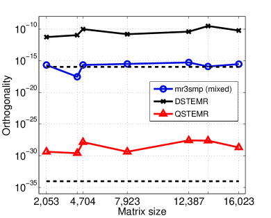
Instead, as we merely require improved accuracy with respect to DSTEMR, we speed up a solver that uses quadruple precision arithmetic internally. The results of such an approach is presented in form of mr3smp (with mixed precision). While computing sufficiently accurate results, Fig. 5.1(b), the reward for the relaxed accuracy requirement is a remarkable up to five-fold speedup compared with the naive approach, Fig. 5.1(a). Although, in a sequential execution, our solver is slower than the standard double precision solver, it comes with two important advantages: robustness and parallelism are increased significantly. Furthermore, the strategy can be adapted to any binary_ x/binary_y solver; in case $y$-bit arithmetic is not that much slower than $x$-bit arithmetic, the mixed precision approach leads to faster executions compared with the standard MRRR. In the next section, we describe our strategy in detail.

5.1.1 Adjusting the algorithm

At this point, it is necessary to recall Theorem 3.1.4 in Section 3.1.2, which specifies the accuracy of any MRRR implementation. The exact values of the parameters in the theorem differ slightly for various implementations of the algorithm and need not to be known in the following analysis. The bounds on the residual norm and orthogonality are theoretical, that is, for a worst case scenario. In practice, the results are smaller than the bounds suggest: with common parameters, realistic practical bounds on the residual norm and on the orthogonality are $n\varepsilon$ and $1000n\varepsilon$, respectively. In order to obtain accuracy similar to that of the best available methods, we need to transform the dependence on $n$ by one on $\sqrt{n}$. Furthermore, it is necessary to reduce the orthogonality by about three orders of magnitude.

Consider the input/output being in a $x$-bit format and the entire computation being performed in $y$-bit arithmetic. Starting from this configuration, we expose the new freedom in the parameter space and justify changes that we make to the algorithm. For example, we identify parts that can be executed in $x$-bit arithmetic, which might be considerably faster.

Assuming $\varepsilon_{y}\ll\varepsilon_{x}$ (again, think of $\varepsilon_{x}\approx 10^{-16}$ and $\varepsilon_{y}\approx 10^{-34}$), we simplify Theorem 3.1.4 by canceling terms that do not contribute significantly even with adjusted parameters (i.e., terms that are comparable to $\varepsilon_{y}$ in magnitude; in particular, we require that $n\varepsilon_{y}\leq\varepsilon_{x}\sqrt{n}$.). In our argumentation, we hide all constants, which anyway correspond to the bounds attainable for a solver purely based on binary_y. For any reasonable implementation of the algorithm, we have the following: $\alpha=\mathcal{O}(\varepsilon_{y})$, $\eta=\mathcal{O}(n\varepsilon_{y})$, $\xi_{\,\downarrow}=\mathcal{O}(\varepsilon_{y})$, $\xi_{\uparrow}=\mathcal{O}(\varepsilon_{y})$. Thus, the orthogonality of the final result is given by

$$|\hat{z}_{i}^{*}\hat{z}_{j}|=\mathcal{O}\left(k_{rs}\frac{n\varepsilon_{y}}{gaptol}+k_{rr}\,d_{max}\,\frac{n\varepsilon_{y}}{gaptol}\right)\,.$$ (5.1)

Similarly, for the bound on the residual norm, we get

$$\lVert M_{root}\,\hat{z}_{i}-\hat{\lambda}_{i}[M_{root}]\,\hat{z}_{i}\rVert=\mathcal{O}\left(\lVert\bar{r}^{(local)}\rVert+\gamma\,spdiam[M_{root}]\right)$$ (5.2)

with $\lVert\bar{r}^{(local)}\rVert\leq k_{rs}\,gap\left(\hat{\lambda}_{i}[M]\right)\frac{n\varepsilon_{y}}{gaptol}$ and $\gamma=\mathcal{O}(k_{elg}\,d_{max}\,n\varepsilon_{y})$.

We now provide a list of changes that can be done to the algorithm. We discuss their effects on performance, parallelism, and memory requirement.

Preprocessing.

We assume scaling and splitting is done as in a solver purely based on $x$-bit floating point arithmetic, see Section 3.2.1. In particular, off-diagonal element $\beta_{i}$ of the input $T$ is set to zero whenever

$$|\beta_{i}|\leq\varepsilon_{x}\sqrt{n}\lVert T\rVert\,,$$

where $n$ and $T$ refer to the unreduced input. We remark that this criterion is less strict than setting elements to zero whenever $|\beta_{i}|\leq\varepsilon_{y}\sqrt{n}\lVert T\rVert$. Splitting the input matrix into submatrices is beneficial for both performance and accuracy as these are mainly determined by the largest submatrix. Throughout this section, we assume that the preprocessing has been done and each subproblem is treated independently by invoking Algorithm 2. In particular, whenever we refer to matrix $T$, it is assumed to be irreducible; whenever we reference the matrix size $n$ in the context of parameter settings, it refers to the size of the processed block.

Choice of form to represent tridiagonals.

For the various forms to represent tridiagonals (e.g., bidiagonal, twisted, or blocked factorizations) and their data (e.g., $N$-, $e$-, or $Z$-representation), different algorithms implement the shift operation in Line 16 of Algorithm 2: $M_{shifted}=M-\tau I$. All these algorithms are stable in the sense that the relation holds exactly if the data for $M_{shifted}$ and $M$ are perturbed element-wise by a relative amount bounded by $\mathcal{O}(\varepsilon_{y})$. The implied constants for the perturbation bounds vary slightly. As $\varepsilon_{y}<\varepsilon_{x}$, instead of concentrating on accuracy issues, we can make our choice based on robustness and performance. A discussion of performance issues related to different forms to represent tridiagonals can be found in [178, 174]. Based on this discussion, it appears that twisted factorizations with $e$-representation seem to be a good choice. As the off-diagonal entries of all the matrices stay the same, they only need to be stored once and are reused during the entire computation.

Random perturbations.

In Line 2 of Algorithm 2, to break up tight clusters, the data of $M_{root}$, $\{x_{1},...,x_{2n-1}\}$, is perturbed element-wise by small random relative amounts: $\tilde{x}_{i}=x_{i}(1+\xi_{i})$ with $|\xi_{i}|\leq\xi$ for all $1\leq i\leq{2n-1}$. In practice, a value like $\xi=8\varepsilon$ is used. Although our data is in binary_y, we can be quite aggressive and adopt $\xi=\varepsilon_{x}$ or a small multiple of it. For $y=2x$, about half of the digits in each entry of the representation are chosen randomly and with high probability, eigenvalues do not agree to many more than $\lceil-\log_{10}{\varepsilon_{x}}\rceil$ digits. This has two major effects: First, together with the changes in $gaptol$ (see below), the probability to encounter large values for $d_{max}$ (say 4 or larger) becomes extremely low. Second, it becomes easier to find suitable shifts such that the resulting representation satisfies the requirements of relative robustness and conditional element growth. The positive impact of small $d_{max}$ on the accuracy is apparent from (5.1) and (5.2). Furthermore, as discussed below, due to limiting $d_{max}$, the computation can be reorganized for efficiency. Although it might look innocent, the more aggressive random perturbations lead to much improved robustness: A detailed discussion can be found in [45, 40].

Classification of the eigenvalues.

Due to the importance of the $gaptol$-parameter, adjusting it to our requirements is key to the success of our approach. The parameter influences nearly all stages of the algorithm; most importantly, the classification of eigenvalues into well-separated and clustered. As already discussed, the choice of gaptol is restricted by the loss of orthogonality that we are willing to accept; in practice, the value is often chosen to be $10^{-3}$ [43]. As we merely require orthogonality of $\varepsilon_{x}\sqrt{n}$, we usually accept more than three orders of magnitude loss of orthogonality. Both terms in (5.1) (and the in practice observed orthogonality) grow as $n\varepsilon_{y}/gaptol$. Consequently, we might select any value satisfying

$$\min\left\{10^{-3},\frac{\varepsilon_{y}\sqrt{n}}{\varepsilon_{x}}\right\}\leq gaptol\leq 10^{-3}\,,$$ (5.3)

for $gaptol$, where the $10^{-3}$ terms are derived from practice and might be altered slightly. Note that $gaptol$ can become as small as $10^{-9}\sqrt{n}$ in the single/double case and $10^{-18}\sqrt{n}$ in the double/quadruple one. If we restrict the analysis to matrices with size $n\leq 10^{6}$, we can choose a constant $gaptol$ as small as $10^{-6}$ and $10^{-15}$ respectively for the single/double and double/quadruple cases.

We use again the double/quadruple case to illustrate the choice of $gaptol$. With $gaptol=10^{-3}$, Fig. 5.2(a) shows a practical upper bound on the orthogonality of MRRR in double precision arithmetic, $1000n\varepsilon$.

(a) Double precision arithmetic.

(b) Quadruple precision arithmetic.

Figure 5.2: Selection of the important parameter $gaptol$. By using higher precision arithmetic we gain freedom in the choice of the parameter.

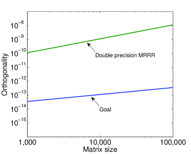
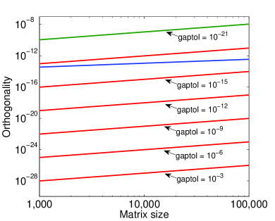
Depending on the specific goal, which for instance growths as $\varepsilon\sqrt{n}$, we aim at improving the orthogonality. If the goal is set as in Fig. 5.2(a), a reader looking at (5.1) might wonder whether it is possible to simply increase $gaptol$ until the accuracy goal is met. Unfortunately, as Fig. 5.3 illustrates, it is not possible to achieve better accuracy by simply selecting a larger value for $gaptol$.

Figure 5.3: Orthogonality of mr3smp (without mixed precision) for various values of $gaptol$. The experiment was performed on test set Application, which is detailed in Appendix D.

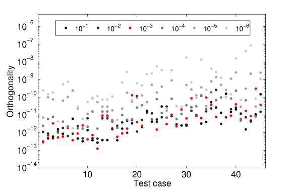
Even with $gaptol=10^{-1}$, no significant accuracy improvement is observed. On the contrary, such a large value of $gaptol$ negatively impacts performance and reliability. If $gaptol$ is too large, it can become impossible to break clusters and a code might fail completely. For this reason, $gaptol<1$ is required and $gaptol\ll 1$ is desired. By Fig. 5.3, even with $gaptol$ being several orders of magnitude smaller than $10^{-3}$, the orthogonality is sufficient for single precision outputs. It is this observation that we exploit in our mixed precision MRRR. For double precision input/output, instead of performing the entire computation in double precision arithmetic, we use quadruple arithmetic. By (5.3), we gain freedom in choosing $gaptol$. We might chose a constant value of $gaptol=10^{-15}$ to fulfill our goal, as depicted in Fig. 5.2(b). Alternatively, we can let $gaptol$ be a function of matrix size $n$ as in the lower bound of (5.3). However, if we do not decrease $gaptol$ to the smallest possible value, by (5.1) and (5.2), we can instead relax other parameters ($k_{rr}$,$k_{rs}$) that influence accuracy.

Returning to the general case of binary_ x/binary_y, with any choice of $gaptol$ complying (5.3), accuracy to the desired level is guaranteed, and there is room to choose the specific value of $gaptol$, as well as other parameters, to optimize performance or parallelism. In particular, by generally reducing the clustering of the eigenvalues, the smallest possible value of $gaptol$ provides the greatest parallelism. As we have done in Section 4.2.5, to quantify this statement, for any matrix, we define clustering $\rho\in[1/n,1]$ formally as the size of the largest cluster divided by the matrix size. The two main advantages in decreasing $\rho$ were also discussed in Section 4.2.5: the work of processing the largest cluster introduces of $\mathcal{O}(\rho n^{2})$ flops is reduced and the potential parallelism is increased. A conservative estimate of the parallelism of a problem is provided by $\rho^{-1}$ (for instance, $\rho=1/n$ implies that the problem is embarrassingly parallel). Matrices with high clustering pose difficulties as they introduce load balancing issues and communication, which can considerably reduce the parallel scalability [162, 161]. Even if we do not desire to guarantee improved accuracy, we can use mixed precisions to enhance parallelism. In this case, the $\sqrt{n}$-dependence on the lower bound for the value of $gaptol$ would be removed and the bound could be loosened by another three orders of magnitude; that is, we might choose a value of $10^{-12}$ and $10^{-21}$ for the single/double and double/quadruple cases, respectively. Most results would still be improved, as the relative gaps of the eigenvalues are often larger than $gaptol$. In addition, we expect that almost all computations become embarrassingly parallel.

As an example, Table 5.2 shows the clustering for double precision Hermite type test matrices of various sizes with four distinct classification criteria: (I) $gaptol=10^{-3}$, (II) $gaptol=10^{-3}$, combined with splitting based on the absolute gap as proposed in [161] to enhance parallelism, (III) $gaptol=10^{-10}$, and (IV) $gaptol=10^{-15}$. As with this example, experience shows that, thanks to a reduced value of $gaptol$ as in criteria III or IV, many problems become embarrassingly parallel and guarantee improved accuracy. In case $\rho=1/n$, $d_{max}$ is zero, which not only benefits accuracy by (5.1) and (5.2), but also has a more dramatic effect: the danger of not finding representations that satisfy the requirements is entirely removed. This follows from the fact that a satisfactory root representation can always be found (e.g., by making $T-\mu I$ definite) and no other representation needs to be computed. Even in cases with $d_{max}>0$, the number of times Line 16 of Algorithm 2 needs to be executed is often considerably reduced.

Criterion	Matrix size
	$2{,}500$	$5{,}000$	$10{,}000$	$20{,}000$
I	0.70	0.86	0.93	0.97
II	0.57	0.73	0.73	0.73
III	4.00e-4	2.00e-4	1.00e-4	5.00e-5
IV	4.00e-4	2.00e-4	1.00e-4	5.00e-5

Table 5.2: The $gaptol$-parameter effect on clustering $\rho\in[1/n,1]$.

On the downside, selecting a smaller $gaptol$ can result in more work in the initial approximation and later refinements – in both cases, eigenvalues must be approximated to relative accuracy of about $gaptol$; as a result, optimal performance is often not achieved for the smallest possible value of $gaptol$. Moreover, as we discuss below, if one is willing to limit the choice of $gaptol$, the approximation of eigenvalues can be done (almost) entirely in $x$-bit arithmetic. If the $y$-bit arithmetic is significantly slower than the $x$-bit one, it might be best to take advantage of the latter. And, as we see below as well, if not the smallest possible value is chosen for $gaptol$, the requirements the intermediate representations must fulfill are relaxed.

Another corollary of adjusting $gaptol$ is slightly hidden: in Line 16 of Algorithm 2, we gain more freedom in selecting $\tau$ such that, at the next iteration, the cluster is broken apart. For instance, when choosing $\tau$ close to one end of the cluster, we are able to “back off” further away than usual from the end of the cluster in cases where we did not find a representation satisfying the requirements in a previous attempt (see Algorithm 8 in Section 3.2.3).

We cannot overemphasize the positive effects an adjusted gaptol has on robustness and parallel scalability. In particular, in parallel computing environments, the smallest value for $gaptol$ can significantly improve the parallel scalability. Since many problems become embarrassingly parallel, the danger of failing is removed entirely.

Arithmetic used to approximate eigenvalues.

In Lines 3 and 17 of Algorithm 2, eigenvalues are respectively computed and refined to a specified relative accuracy. In both cases, we are given a representation, which we call $M_{y}$ henceforth, and an index set $\mathcal{I}$ that indicates the eigenvalues that need to be approximated. When the $y$-bit arithmetic is much slower than the $x$-bit one (say a factor 10 or more), the use of the latter is preferred: One creates a temporary copy of $M_{y}$ in binary_ x – called $M_{x}$ henceforth – that is used for the eigenvalue computation in $x$-bit arithmetic. The creation of $M_{x}$ corresponds to an element-wise relative perturbation of $M_{y}$ bounded by $\varepsilon_{x}$. By the relative robustness of $M_{y}$,

$$\lvert\lambda_{i}[M_{x}]-\lambda_{i}[M_{y}]\rvert\leq k_{rr}n\varepsilon_{x}\lvert\lambda_{i}[M_{y}]\rvert\,.$$ (5.4)

For instance, bisection can be used to compute eigenvalue approximations $\hat{\lambda}_{i}[M_{x}]$ to high relative accuracy, after which $M_{x}$ is discarded. As casting the result back to binary_y causes no additional error, it is $\hat{\lambda}_{i}[M_{y}]=\hat{\lambda}_{i}[M_{x}]$ and

$$\lvert\hat{\lambda}_{i}[M_{y}]-\lambda_{i}[M_{x}]\rvert\leq k_{bi}n\varepsilon_{x}\lvert\lambda_{i}[M_{x}]\rvert\,,$$

where $k_{bi}$ is a constant given by the bisection method. To first order, by the triangle inequality, it holds

$$\lvert\hat{\lambda}_{i}[M_{y}]-\lambda_{i}[M_{y}]\rvert\leq\left(k_{rr}+k_{bi}\right)n\varepsilon_{x}\lvert\lambda_{i}[M_{y}]\rvert\,.$$ (5.5)

Provided $\left(k_{rr}+k_{bi}\right)n\varepsilon_{x}\lesssim gaptol$, $x$-bit arithmetic can be used to approximate the eigenvalues. Thus, an additional constraint on both the size $n$ and $gaptol$ arises: Given $gaptol$, we must limit the matrix size up to which we can do the computation purely in $x$-bit arithmetic. Similarly, for a given matrix size, we need to adjust the lower bound on $gaptol$ in (5.3). As an example, if say $k_{rr}\leq 10$, $k_{bi}\leq 10$, $n\leq 10^{6}$, and $\varepsilon_{x}=\varepsilon_{d}=2^{-53}$, it is required that that $gaptol\gtrsim 10^{-10}$. When resorting to $x$-bit arithmetic or if $gaptol$ is chosen too small, one might respectively verify or refine the result of the $x$-bit eigenvalue computation using $y$-bit arithmetic without significant costs.

Requirements on the representations.

As long as $k_{elg}n\varepsilon_{y}\ll\varepsilon_{x}\sqrt{n}$, by (5.2), the residual with respect the $M_{root}$ is mainly influenced by the local residual. In our mixed precision approach, without loss of accuracy, it is possible to allow for

$$k_{elg}\leq\max\left\{10,\frac{\varepsilon_{x}}{\varepsilon_{y}\sqrt{n}}\right\}\,,$$ (5.6)

where we assumed 10 was the original value of $k_{elg}$. As a result, the requirement on the conditional element growth is considerably relaxed. For instance, in the single/double and double/quadruple cases, assuming $n\leq 10^{6}$, bounds on $k_{elg}$ of about $10^{6}$ and $10^{15}$ are sufficient, respectively. If $gaptol$ is not chosen as small as possible, the bound on $k_{rr}$ can be loosened in a similar fashion:

$$k_{rr}\leq\max\left\{10,\frac{\varepsilon_{x}}{\varepsilon_{y}\sqrt{n}}\cdot gaptol\right\}\,.$$ (5.7)

As an example, in the double/quadruple case, assuming $n\leq 10^{6}$ and $gaptol$ set to $10^{-10}$, $k_{rr}\leq 10^{5}$ would be sufficient to ensure accuracy.

Rayleigh quotient iteration.

Our willingness to lose orthogonality up to a certain level, which is noticeable in the lower bound on $gaptol$, is also reflected in stopping criterion for RQI, which is given by (3.16). As $n\varepsilon_{y}/gaptol\leq\varepsilon_{x}\sqrt{n}$, we can stop the RQI when

$$\lVert\bar{r}^{(local)}\rVert\leq k_{rs}\cdot gap\left(\hat{\lambda}_{i}[M]\right)\,\varepsilon_{x}\sqrt{n}\,,$$ (5.8)

where $k_{rs}$ is $\mathcal{O}(1)$. In practice, we take $k_{rs}\approx 1$ or even $k_{rs}\approx 1/\sqrt{n}$. As a consequence, the iteration is stopped earlier on and overall work reduced.

As a side note: In the rare cases where RQI fails to converge (or as a general alternative to RQI), we commonly resort to bisection to approximate the eigenvalue $\lambda_{i}$ and then use only one step of RQI (with or without applying the correction term). In the worst case, we require the eigenvalue to be approximated to high relative accuracy, $|\hat{\lambda}_{i}-\lambda_{i}|=\mathcal{O}(n\varepsilon_{y}|\lambda_{i}|)$ [44]. With mixed precision, we can relax the condition to $|\hat{\lambda}_{i}-\lambda_{i}|=\mathcal{O}(\varepsilon_{x}\sqrt{n}|\lambda_{i}|\,gaptol)$, which is less restrictive if $gaptol$ is not chosen as small as possible. If $relgap(\hat{\lambda}_{i})\gg gaptol$, the restriction on the accuracy of the approximated eigenvalue can be lifted even further [174].

Traversal of the representation tree.

Thanks to the random perturbation of the root representation and a properly adjusted $gaptol$-parameter, we rarely expect to see large values for $d_{max}$. For all practical purposes, in the case of $y=2x$, we may assume $d_{max}\leq 2$. As a result, the computation can be rearranged, as discussed in [175] and summarized in the following: To bound the memory consumption, a breath-first strategy such as in Algorithm 2 is used; see for instance in [46, 123]. This means that, at any level of the representation tree, all singletons are processed before the clusters. A depth-first strategy would instead process entire clusters, with the only disadvantage that meanwhile up to $d_{max}$ representations need to be kept in memory. If $d_{max}$ is limited as in our case, the depth-first strategy can be used without disadvantage. In fact, a depth-first strategy brings two advantages: ($i$) copying representations to and from the eigenvector matrix is avoided entirely (see the next section on the benefit for the mixed precision MRRR) and ($ii$) if at some point in the computation no suitable representation is found, there is the possibility of backtracking, that is, we can process the cluster again by choosing different shifts at a higher level of the representation tree. For these reasons, in the mixed precision MRRR, a depth-first strategy is preferred.

5.1.2 Memory cost

We stress both input and output are in binary_ x format; only internally (i.e., hidden to a user) $y$-bit arithmetic is used. The memory management of an actual implementation of MRRR is affected by the fact that output matrix $Z\in\mathbb{R}^{n\times k}$, containing the desired eigenvectors, is commonly used as intermediate workspace. Since $Z$ is in binary_ x format, whenever $y>x$, the workspace is not sufficient anymore for its customary use: For each cluster, a representation is stored in the corresponding columns of $Z$ [46, 123]. As these representations consist of $2n-1$ binary_y numbers, this approach is generally not applicable. If we restrict to $y\leq 2x$, we can store the $2n-1$ binary_y numbers whenever a cluster of size four and more is encountered. Thus, the computation must be reorganized so that at least clusters containing less than four eigenvalues are processed without storing any data in $Z$ temporarily. In fact, using a depth-first strategy, we remove the need to use $Z$ as temporary storage entirely. Furthermore, immediately after computing an eigenvector in binary_y, it is converted to binary_ x, written into $Z$, and discarded. Consequently, while our approach slightly increases the memory usage, we do not require much more memory: with $p$ denoting the level of parallelism (i.e., number of threads or processes used), the mixed precision MRRR still needs only $\mathcal{O}(pn)$ binary_ x floating point numbers extra workspace.

5.2 Practical aspects

We have implemented the mixed precision MRRR for three cases: single/double, double/extended, and double/quadruple. The first solver accepts single precision input and produces single precision output, but internally uses double precision. The other two are for double precision input/output. The performance of the solvers, compared with the traditional implementation, depends entirely on the difference in speed between the two involved arithmetic. If the higher precision arithmetic is not much slower (say less than a factor four), the approach is expected to work well, even for sequential executions and relatively small matrices. If the higher precision arithmetic is considerably slower, the mixed precision MRRR might still perform well for large matrices or, due to increased parallelism, when executed on highly parallel systems. Our target application is the computation of a subset of eigenpairs of large-scale dense Hermitian matrices. For such a scenario, we tolerate a slowdown of the tridiagonal eigensolver due to the use of mixed precisions without affecting overall performance significantly [124, 125].

5.2.1 Implementations

In Section 5.3, we present experimental results of our implementations. All mixed precision implementations are based on mr3smp, presented in Chapter 4, and use $N$-representations of lower bidiagonal factorizations. As discussed in Algorithm 4 in Section 3.2, bisection is used for the initial eigenvalue computation if a small subset of $k$ eigenpairs is requested or if the number of executing threads exceeds $12k/n$. If all eigenpairs are requested and the number of threads is less than 12, the fast sequential dqds algorithm [60, 120] is used instead of bisection. As a consequence, speedups compared to the sequential execution appear less than perfect even for an embarrassingly parallel computation.

As several design decisions can be made and the run time depends on both the specific input and the architecture, optimizing a code for performance is non-trivial. However, we can choose settings in a way that in general yields good, but not necessarily optimal, performance. For instance, on a highly parallel machine one would pick a small value for $gaptol$ to increase parallelism. For testing purposes, we disabled the classification criterion based on the absolute gaps of the eigenvalues proposed in [161], which might reduce clustering even further (it has no consequences for our test cases shown in the next section).

For now, we did not relax the requirements on the representations according to (5.6) and (5.7); we only benefit from the possibility of doing so indirectly: As shown in Algorithm 8 in Section 3.2, if no suitable representation is found, a good candidate is chosen, which might fulfill the relaxed requirements. In the following, we provide additional comments to all of the mixed precision solvers individually.

Single/double.

With widespread language and hardware support for double precision, the mixed precision MRRR is most easily implemented for the single/double case. In our test implementation, we fixed $gaptol$ to $10^{-5}$. When bisection is used, the initial approximation of eigenvalues is done to a relative accuracy of $10^{-2}\cdot gaptol$; the same tolerance is used for the later refinements. We additionally altered the computation of compared with mr3smp: Thanks to the reduced clustering, the initial eigenvalue approximation often becomes the most expensive part of the computation. In order to achieve better load balancing in this stage, we reduced the granularity of the tasks and used dynamic scheduling of tasks.

As on most machines the double precision arithmetic is not more than a factor two slower than the single precision one, we carry out all computations in the former. Data conversion is only necessary when reading the input and writing the output. As a result, compared with a double precision solver using a depth-first strategy, merely a number of convergence criteria and thresholds must be adjusted, and the RQI must be performed using a temporary vector that is, after convergence, written into the output eigenvector matrix. The mixed precision code closely resembles a conventional double precision implementation of MRRR.

Double/extended.

Many current architectures have hardware support for a 80-bit extended floating point format (see Table 5.1 in Section 5.1). As the unit roundoff is only about three orders of magnitude smaller than for double precision, we can improve the accuracy of MRRR by this amount. For matrices of moderate size, the accuracy becomes comparable to that of the best methods (see Appendix F). The main advantage of the extended format is that, compared with double precision, its arithmetic comes without any or only a small loss in speed. On the downside, we cannot make any further adjustments in the algorithm to positively effect its robustness and parallelism. We do not include test results in the experimental section; however, we tested the approach and results can be found in Appendix F.

Double/quadruple.

As quadruple precision arithmetic is not widely supported by today’s processors, we had to resort to a rather slow software-simulated arithmetic. For this reason, we used double precision for the initial approximation and for the refinement of the eigenvalues. The necessary intermediate data conversions make the mixed precision approach slightly more complicated to implement than the single/double one. We used the value $10^{-10}$ for $gaptol$ in our tests. Further details can be found in [125].

5.2.2 Portability

The biggest problem of the mixed precision approach is a potential lack of support for the involved data types. As single and double precisions are supported by virtually all machines, languages, and compilers, the mixed precision approach can be incorporated to any linear algebra library for single precision input/output. However, for double precision input/output, we need to resort to either extended or quadruple precision. Not all architectures, languages, and compilers support these formats. For instance, the 80-bit floating point format is not supported by all processors. Furthermore, while the FORTRAN REAL*10 data type is a non-standard feature of the language and is not supported by all compilers, a C/C++ code can use the standardized long double data type (introduced in ISO C99) that achieves the desired result on most architectures that support 80-bit arithmetic. For the use of quadruple precision, there are presently two major drawbacks: ($i$) it is usually not supported in hardware, which means that one has to resort to a rather slow software-simulated arithmetic, and ($ii$) the support from compilers and languages is rather limited. While FORTRAN has a REAL*16 data type, the quadruple precision data type in C/C++ is compiler-dependent: for instance, there exist the  float128 and  Quad data types for the GNU and Intel compilers, respectively. An external library implementing the software arithmetic might be used for portability. In all cases, the performance of quadruple arithmetic depends on its specific implementation. It is however likely that the hardware/software support for quadruple precision will be improved in the near future.

5.2.3 Robustness

The mixed precision MRRR provides improved robustness. To quantify the robustness of an eigensolver, as discussed in Section 2.5, we propose the following measure: For a given test set of matrices, TestSet, the robustness $\phi$ is expressed as

$$\phi(\mbox{\sc TestSet})=1-\frac{\mbox{\sc NumFailures}}{|\mbox{\sc TestSet}|}\,$$ (5.9)

where NumFailures is the number of inputs for which the method “fails”. At this point, we elaborate on what constitutes as failure.

If the output does not comply with even the theoretical error bounds (which includes failing to return a result at all), one or more assumptions in the derivation of the bounds are not satisfied. For MRRR, usually a representation that is not relative robustness is accepted as an RRR. We therefore suggest that cases in which at least one representation is accepted without passing the test for relative robustness are considered failures. Furthermore, for any method, we might be more strict and classify an execution as troublesome if the output exceeds practical error bounds as well, which often signals problems earlier on.

If we use such a strict standard to measure robustness, we believe that use of mixed precisions might be an important ingredient for MRRR to achieve robustness comparable to the most reliable solvers (in particular, implementations of QR). A number of improvements of MRRR’s robustness are proposed in [174] (e.g., changing the form to represent intermediate tridiagonals, using of the substructure of clusters to obtain more reliable envelope information, and allowing shifts inside clusters). We remark that our implementations of the mixed precision MRRR do not implement all of them, but since these measures are orthogonal to our approach, they can and should be additionally adopted for maximal robustness.

5.3 Experimental results

All tests, in this section, were run on an multiprocessors system comprising four eight-core Intel Xeon X7550 Beckton processors, with a nominal clock speed of 2.0 GHz. Subsequently, we refer to this machine as Beckton (see Appendix C). We used LAPACK version 3.4.2 and linked the library with the vendor-tuned MKL BLAS version 12.1. In addition to the results for LAPACK’s routines and our mixed precision solvers, which we call mr3smp (mixed) subsequently, we also include results for mr3smp without mixed precisions. All routines of this experiment were compiled with Intel’s compiler version 12.1 and optimization level -O3 enabled. Although we present only results for computing all eigenpairs (LAPACK’s DC does not allow the computation of subsets), we mention that MRRR’s strength and main application lies in the computation of subsets of eigenpairs.

For our tests, we used matrices of size ranging from $2{,}500$ to $20{,}000$ (in steps of $2{,}500$) of six different types: uniform eigenvalue distribution, geometric eigenvalue distribution, 1–2–1, Clement, Wilkinson, and Hermite. The dimension of the Wilkinson type matrices is $n+1$, as they are only defined for odd sizes. Details on these matrix types can be found in Appendix D. To help the exposition of the results, in the accuracy plots, the matrices are sorted by type first and then by size; vice versa, in the plots relative to timings, the matrices are sorted by size first and then by type. Subsequently, we call the test set Artificial.

We use a second test set, Application, which consists of 45 matrices arising in scientific applications. Most matrices, , listed in Appendix D, are part of the publicly available Stetester suite [104] and range from $1{,}074$ to $8{,}012$ in size.

5.3.1 Tridiagonal matrices

For the Artificial matrices in single precision, Figs. 5.4 and 5.5 shows timing and accuracy results, respectively.

(a) Execution time: sequential.

(b) Execution time: multi-threaded.

Figure 5.4: Timings for test set Artificial on Beckton. The results of LAPACK’s SSTEMR (MRRR) and SSTEDC (Divide & Conquer) are used as a reference.

(a) Largest residual norm.

(b) Orthogonality.

Figure 5.5: Accuracy for test set Artificial. The largest residual norm and the orthogonality are measured as in (2.5). The results of LAPACK’s SSTEMR (MRRR) and SSTEDC (Divide & Conquer) are used as a reference. The dotted lines indicate unit roundoff $\varepsilon_{s}$.

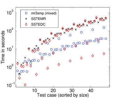
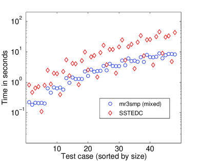
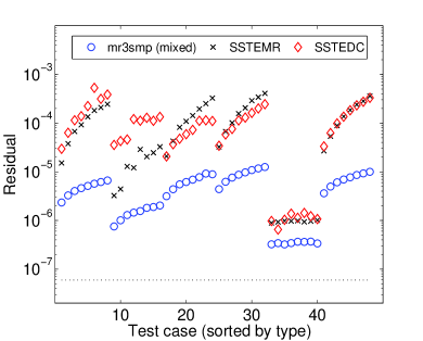
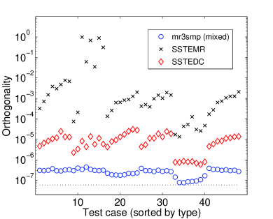
As a reference, we include results for LAPACK’s SSTEMR (MRRR) and SSTEDC (Divide & Conquer). Even in a sequential execution, Fig. 5.4(a), our mixed precision solver mr3smp (mixed) is up to an order of magnitude faster than LAPACK’s SSTEMR. For one type of matrices, SSTEDC is considerably faster than for all the others. These are the Wilkinson matrices, which represent a class of matrices that allow for heavy deflation within the Divide & Conquer approach. For all other matrices, which do not allow such extensive deflation, our solver is usually faster than SSTEDC. As seen in Fig. 5.4(b), in a parallel execution with one thread/core, the performance gap for the Wilkinson matrices almost entirely vanishes, while for the other matrices mr3smp (mixed) remains faster than SSTEDC. As depicted in Fig. 5.5, our routine is not only as accurate as desired, but it is the most accurate. In particular, for the large matrices with geometric eigenvalue distribution, SSTEMR even fails to return numerically orthogonal eigenvectors, while mr3smp (mixed) returns accurate results.

The faster execution of the mixed precision solver relative to SSTEMR is explained by Fig 5.6(a), which shows the maximal depth of the representation tree, $d_{max}$.

(a) Single precision.

(b) Double precision.

Figure 5.6: Maximal depth of the representation tree, $d_{max}$.

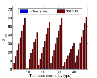
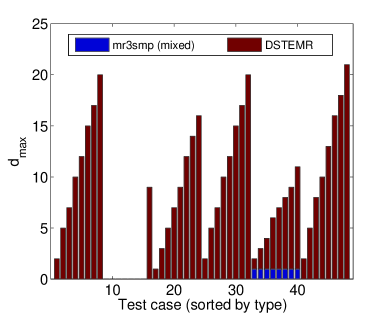
A standard MRRR using single precision requires significant effort to construct a sequence of relative robust representations from which the eigenpairs are computed. In contrast, using mixed precisions, $d_{max}$ is limited to one – for all but two matrix types, it is even zero.

If we consider each computation in which MRRR accepts at least one representation not passing the test for relative robustness as a failure, for SSTEMR, 38 out of the 48 test cases are problematic and $\phi(\mbox{\sc Artificial})\approx 0.21$. The number indicates that in almost 80% of the test cases, SSTEMR might produce erroneous results. However, only in three out of the 38 problematic cases this is reflected in an orthogonality exceeding $n\varepsilon/gaptol$. Consequently, an improved test for relative robustness, such as proposed in [174], could probably reduce the number of failures significantly. Even without altering the selection of RRRs, mr3smp (mixed) was able to find suitable representations and $\phi(\mbox{\sc Artificial})=1$. Furthermore, the orthogonality is bounded by $\varepsilon\sqrt{n}$ as desired. For single precision input/output arguments, we obtain a solver that is more accurate and faster than the original single precision solver. In addition, it is more robust and more scalable.

We now turn our attention to double precision input/output, for which timings and accuracy are presented in Figs. 5.7 and 5.8, respectively.

(a) Execution time: sequential.

(b) Execution time: multi-threaded.

Figure 5.7: Timings for test set Artificial on Beckton. The results of LAPACK’s DSTEMR (MRRR) and DSTEDC (Divide & Conquer), as well as the multi-threaded mr3smp as introduced Chapter 4, are used as a reference.

(a) Largest residual norm.

(b) Orthogonality.

Figure 5.8: Accuracy for test set Artificial. The largest residual norm and the orthogonality are measured as in (2.5). The results of mr3smp and LAPACK’s DSTEDC (Divide & Conquer) are used as a reference. In general, mr3smp obtains accuracy equivalent to LAPACK’s DSTEMR (MRRR). The dotted lines indicate unit roundoff $\varepsilon_{d}$.

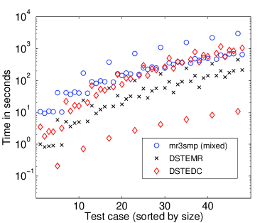
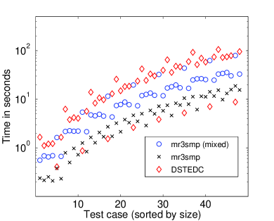
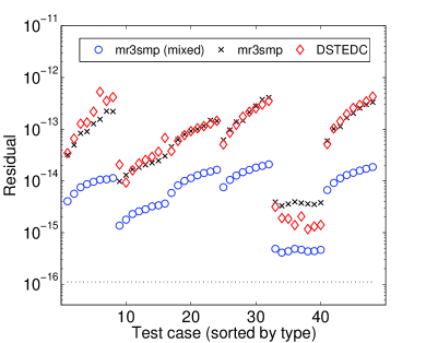
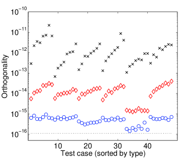
We included the results for mr3smp without mixed precisions, which in the sequential case is just a wrapper to LAPACK’s DSTEMR. In general, mr3smp obtains accuracy equivalent to DSTEMR.

Figure 5.7(a) shows timings for sequential executions: mr3smp (mixed) is slower than DSTEMR, which is not a surprise, as we make use of software-simulated quadruple precision arithmetic. What might be a surprise is that even with the use of such slow arithmetic, for large matrices, mr3smp (mixed) is often as fast as DSTEDC. As in the single precision case, only for matrices that allow heavy deflation, DSTEDC is considerably faster. As Fig. 5.7(b) shows, for parallel executions, such performance difference reduces and is expected to eventually vanish, see also Fig. 4.10(b) in Section 4.2.3. For matrices that do not allow for extensive deflation, mr3smp (mixed) is about a factor two faster than DSTEDC.

The reason that mr3smp (mixed) is, despite its use of software-simulated arithmetic, not much slower than DSTEMR is depicted in Fig. 5.6(b). While for DSTEMR $d_{max}$ is as large as 21, for mr3smp (mixed), we have $d_{max}\leq 1$. In fact, for all but the Wilkinson type matrices, we have $d_{max}$ equals zero and as a consequence: no danger of failing to find suitable representations and embarrassingly parallel computation. To illustrate the difference between the standard MRRR and the mixed precision variant, we report the clustering $\rho\in[1/n,1]$ for various matrices in Table 5.3.

Matrix	Routine	Matrix size
		2,500	5,000	10,000	20,000
Uniform	DSTEMR	0.60	0.80	0.90	0.95
	mr3smp (mixed)	4.00e-4	2.00e-4	1.00e-4	5.00e-5
Geometric	DSTEMR	4.00e-4	2.00e-4	1.00e-4	0.87
	mr3smp (mixed)	4.00e-4	2.00e-4	1.00e-4	5.00e-5
1–2–1	DSTEMR	0.43	0.64	0.81	0.90
	mr3smp (mixed)	4.00e-4	2.00e-4	1.00e-4	5.00e-5
Clement	DSTEMR	0.60	0.80	0.90	0.95
	mr3smp (mixed)	4.00e-4	2.00e-4	1.00e-4	5.00e-5
Wilkinson	DSTEMR	0.20	0.60	0.80	0.90
	mr3smp (mixed)	8.00e-4	4.00e-4	2.00e-4	1.00e-4

Table 5.3: Clustering $\rho\in[1/n,1]$ for different types of test matrices. The results for Hermite type matrices were already presented in Table 5.2 as criterion I (DSTEMR) and III (mr3smp with mixed precision).

(Recall that the smaller $\rho$ the more natural parallelism is provided by the problem.) DSTEMR is confronted with significant clustering. In contrast, in the mixed precision solver, for all but the Wilkinson matrices, $\rho=1/n$. For Wilkinson matrices, clustering $\rho$ was limited to $2/n$, which still implies ample parallelism. The data suggest that our approach is especially well-suited for highly parallel systems. In particular, solvers for distributed-memory systems should greatly benefit from better load balancing and reduced communication.

In addition to enhanced parallelism, robustness is improved. For DSTEMR, we have $\phi(\mbox{\sc Artificial})\approx 0.40$ and, consequently, the accuracy of DSTEMR might have turned out problematic for about 60% of the inputs. However, no execution actually resulted in insufficient accuracy. For mr3smp (mixed), we have $\phi(\mbox{\sc Artificial})=1$, that is, all computed representations passed the test for relative robustness. Furthermore, as Fig. 5.8 shows, mr3smp (mixed) attains excellent accuracy; both the residuals and the orthogonality are improved to the desired level. In fact, the latter is several orders of magnitude better than what can be expected by the standard MRRR.

5.3.2 Real symmetric dense matrices

For single precision inputs [Fig. 5.4] or for double precision inputs in a parallel setting [Fig. 5.7(b)], in terms of execution time, our mixed precision tridiagonal eigensolver is highly competitive with Divide & Conquer and the standard MRRR. Hence, when used in context of dense Hermitian eigenproblems, the accuracy improvement of the tridiagonal stage carry over to the dense problem without any performance penalty. Even for sequential executions with double precision inputs [Fig. 5.7(a)], the slowdown due to mixed precisions is often not dramatic. The reason is that, to compute $k$ eigenpairs, MRRR only requires $\mathcal{O}(kn)$ arithmetic operations, while the reduction to tridiagonal form requires $\mathcal{O}(n^{3})$ operations. Consequently, the time spent in the tridiagonal stage is asymptotically negligible.

In Figs. 5.9 and 5.10, we present respectively timings and accuracy for real symmetric matrices in single precision.

(a) Execution time: sequential.

(b) Execution time: multi-threaded.

Figure 5.9: Timings for test set Artificial on Beckton. The results of LAPACK’s SSYEVR (MRRR) and SSYEVD (Divide & Conquer) are used as a reference. In a multi-threaded execution, SSYEVR is slower than the other two routines, as it makes use of the sequential routine SSTEMR.

(a) Largest residual norm.

(b) Orthogonality.

Figure 5.10: Accuracy for test set Artificial. The largest residual norm and the orthogonality are measured as in (2.5). The results of LAPACK’s SSYEVR (MRRR) and SSYEVD (Divide & Conquer) are used as a reference. The dotted line indicates unit roundoff $\varepsilon_{s}$.

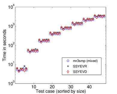
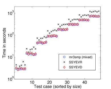
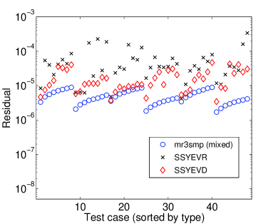
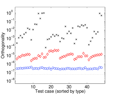
The matrices are generated by applying random orthogonal similarity transformations to the tridiagonal matrices of the previous experiments: $A=QTQ^{*}$, with random orthogonal matrix $Q\in\mathbb{R}^{n\times n}$. By Theorem 3.1.2, the error in the eigenvalue is a lower bound on the residual norm: $|\hat{\lambda}-\lambda|\leq\lVert A\hat{x}-\hat{\lambda}\hat{x}\rVert$. In general, we can only hope to compute eigenvalues with an $\mathcal{O}(n\varepsilon\lVert A\rVert)$ error and therefore do not expect improvements in the residuals. However, the improvements in the orthogonality directly translate to the dense eigenproblem. Figure 5.10 demonstrates that excellent accuracy is achieved with the mixed precision approach. On top of that, as shown in Fig. 5.9, mr3smp (mixed) is faster than LAPACK’s SSYEVR – sequentially and multi-threaded. In a multi-threaded execution, it becomes apparent that the tridiagonal stage of SSYEVR, SSTEMR, is not parallelized. However, the vast majority of time is spent in the reduction to tridiagonal form and the backtransformation of the eigenvectors. For a comparison of Figs. 5.9(a) and 5.9(b), we remark that the reduction to tridiagonal form, SSYTRD, does not scale and limits the speedup of a parallel execution. A similar experiment using the Application matrices can be found in Appendix G. The experiment underpins that generally good performance and accuracy can be expected for single precision input/output.

Interestingly, if we allow an orthogonality of up to $n\varepsilon/gaptol$ (or close to that), SSYEVR cannot be used reliably for matrices as large as in our test set. The orthogonality bound is close to or even exceeds one. Consequently, the applicability of MRRR is limited. However, in certain situations, it might be beneficial to use single precision computations for such large matrices: the memory requirement and execution time of a solver is reduced by a factor two. The mixed precision MRRR does not introduce such a tight restriction on the matrix size. As shown in Fig. 5.10, even for large matrices, mr3smp (mixed) delivers accuracy to a level that might be expected.

We now turn our attention again to double precision input/output.

(a) Execution time: sequential.

(b) Execution time: multi-threaded.

Figure 5.11: Timings for test set Artificial on Beckton. The results of LAPACK’s DSYEVR (MRRR) and DSYEVD (Divide & Conquer) are used as a reference.

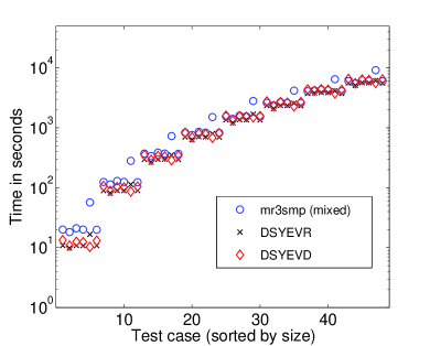
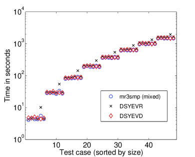
The timings for tridiagonal inputs in Fig. 5.7(a) indicate that, in sequential execution, for small matrix sizes, our approach introduces overhead. However, as seen in Fig. 5.11(a), for dense eigenproblems, the execution time is effected less severely. In a parallel execution, Fig. 5.11(b), mr3smp (mixed) is competitive even for smaller matrices. In all cases, the improved accuracy of the tridiagonal stage carries over to the dense eigenproblem, as exemplified by Fig. 5.12.

(a) Largest residual norm.

(b) Orthogonality.

Figure 5.12: Accuracy for test set Artificial. The largest residual norm and the orthogonality are measured as in (2.5). The results of LAPACK’s DSYEVR (MRRR) and DSYEVD (Divide & Conquer) are used as a reference. The dotted lines indicate unit roundoff $\varepsilon_{d}$.

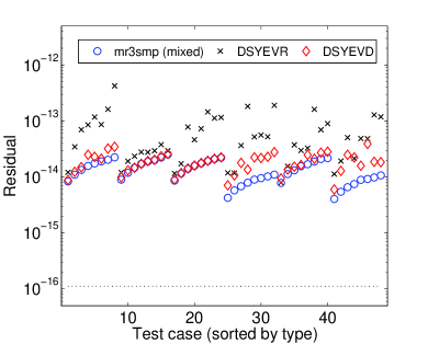
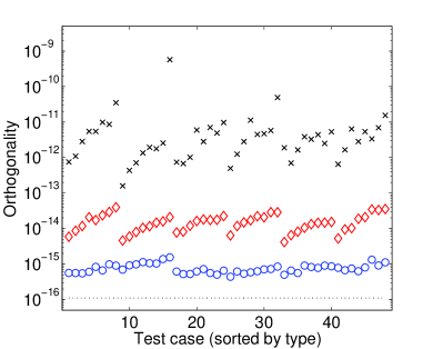
We also performed a similar experiment for the Application matrices. The results are presented in Appendix G and support two previously made statements: First, for small matrices, the sequential execution is slower than DSYEVR, but the performance gap reduces as the matrix size increases. Second, the accuracy improvements are usually limited to the orthogonality; the residuals are often comparable for all solvers.

The above tests were limited to computing all eigenpairs of real symmetric matrices. If the matrices were complex-valued and/or only a subset of eigenpairs were computed, the mixed precision approach would work even better. As a result, using mixed precisions, we obtain eigensolvers for large-scale Hermitian eigenproblems that are fast and accurate. In particular, our solvers compete with the fast Divide & Conquer method when all eigenpairs are computed and are faster when only a small subset of eigenpairs is desired. Furthermore, they are accurate and promise to be highly scalable.

Chapter 6 Conclusions

Recent developments in computer hardware dictate that programs need to make efficient use of the ever growing parallelism in order to improve their performance. We concentrated on how eigensolvers based on the algorithm of Multiple Relatively Robust Representations efficiently exploit modern parallel computers.

For today’s multi-core and future many-core architectures, we presented a parallelization strategy, MR³-SMP, that breaks the computation into tasks to be executed by multiple threads. The tasks are both created and scheduled dynamically. While a static division of work would introduce smaller overheads, the dynamic approach is flexible and produces remarkable workload balancing. Our approach matches or outperforms parallel routines designed for distributed-memory architectures as well as all the eigensolvers in LAPACK and Intel’s MKL.

For massively parallel supercomputers, which are themselves built out of multi-core processors, we created an eigensolver, PMRRR, that merges the previously introduced task-based approach with a parallelization using message-passing. With a proper scheduling of tasks and the use of non-blocking communication, we are able to achieve better scalability than all the solvers included in ScaLAPACK. Furthermore, experiments indicate that our solver is among the fastest tridiagonal eigensolvers available.

PMRRR was integrated in the publicly available Elemental library for the solution of standard and generalized dense Hermitian eigenproblems. A performance study on two supercomputers at the Research Center Jülich, Germany, revealed that Elemental’s eigensolvers outperform the widely used ScaLAPACK – sometimes significantly. For highly parallel executions, the tridiagonal stage of ScaLAPACK’s eigensolvers contributed considerably to the overall run time. In contrast, Elemental’s tridiagonal stage, which makes use of PMRRR, scales well and, in all experiments, was negligible in terms of execution time. As with the tridiagonal stage, for standard and generalized dense Hermitian eigenproblems, much of Elemental’s performance advantage over ScaLAPACK comes from a better scalability in the various stages of the computation.

Although fast, the accuracy of MRRR-based eigensolvers can be several orders of magnitude worse compared with solvers based on the Divide & Conquer or the QR algorithms. Additionally, for solvers targeting distributed-memory systems, input matrices with highly clustered eigenvalues introduce communication and lead to load imbalance. For such matrices, the parallel scalability is limited. Even worse, as every now and then a crucial assumption in the proof of MRRR’s correctness cannot be verified, the accuracy of the output is not always guaranteed.

To address the limitations of MRRR, we introduced a mixed precision variant of the algorithm. Our approach adopts a new perspective: Given input/output arguments in a binary_ x floating point format, internally to the algorithm, we use a higher precision binary_y arithmetic to obtain the desired accuracy. The use of mixed precisions provides us with more freedom to choose important parameters of the algorithm. In particular, while meeting more demanding accuracy goals, we reduce the operation count, increase robustness, and improve parallelism.

Combining all the techniques presented in this thesis, eigensolvers based on our mixed precision MRRR are not only as accurate as eigensolvers based on the Divide & Conquer or the QR algorithms, but – in many circumstances – are also faster or even faster than solvers using a conventional MRRR implementation. Due to their superior scalability, such a statement is particularly true for massively parallel computing environments.

Appendix A A list of (Sca)LAPACK’s Eigensolvers

A.1 (Sca)LAPACK’s symmetric tridiagonal eigensolvers

As LAPACK is the de facto standard for dense linear algebra computations, we frequently show performance and accuracy results for its implementations of various algorithms. In Table A.1, we compile a list of currently available routines for the STEP within LAPACK. The placeholder x in the names stands for one of the following: S single precision, C single precision complex, D double precision, or Z double precision complex.

Method	Routine	Functionality	Subset	Reference
Bisection	xSTEBZ	EW	Yes	[86]
Inverse Iteration	xSTEIN	EV	Yes	[84, 41]
$\sqrt{\;\,}$-free QR Iteration	xSTERF	EW	No	[111, 134, 114]
QR Iteration (positive def.)	xPTEQR	EW + EV	No	[36, 60]
QR Iteration	xSTEQR	EW + EV	No	[22]
Divide and Conquer	xSTEDC	EW + EV	No	[136]
MRRR	xSTEMR	EW + EV	Yes	[46]

Table A.1: LAPACK routines for the STEP. EW means eigenvalues only, EV means eigenvectors only, and EW + EV means eigenvalues and optionally eigenvectors. Additionally, xSTEGR exist, which is just a wrapper to xSTEMR.

The routines are mainly used through four different expert routines: xSTEV, xSTEVX, xSTEVD, and xSTEVR. They work as follows:

• xSTEV uses QR Iteration. If only eigenvalues are desired, the routine calls the square-root free variant xSTERF and, otherwise, it calls xSTEQR.

• xSTEVX uses bisection and inverse iteration. The routine calls xSTEBZ, followed by xSTEIN.

• xSTEVD uses Divide & Conquer. If only eigenvalues are desired, the routine uses QR (xSTERF) by default and, otherwise, calls xSTEDC.

• xSTEVR uses MRRR. If all eigenvalues are requested, the routine uses QR (xSTERF), and, if a subset of eigenvalues is required, it uses bisection (xSTEBZ). If all eigenpairs are requested, the routine uses xSTEMR, otherwise, it makes use of bisection and inverse iteration (xSTEBZ and xSTEIN).

ScaLAPACK contains a subset of the above methods. By convention, the corresponding ScaLAPACK routines have a preceding P in their names, indicating the parallel version. Table A.2 gives an overview of the available routines.

Method	Routine	Functionality	Subset	Reference
Bisection	PxSTEBZ	EW	Yes	[33]
Inverse Iteration	PxSTEIN	EV	Yes	[38]
Divide and Conquer	PxSTEDC	EW + EV	No	[151]

Table A.2: ScaLAPACK routines for the STEP. EW means eigenvalues only, EV means eigenvectors only, and EW + EV means eigenvalues and optionally eigenvectors.

ScaLAPACK also implements the QR algorithm and MRRR (included in 2011), but they are not encapsulated in a separate routine. They are however used for the solution of the HEP. We use the name PxSTEMR for the tridiagonal MRRR.

A.2 (Sca)LAPACK’s Hermitian eigensolvers

Table A.3 lists all routines for the standard HEP. Similar routines for packed storage and banded matrices exist, but are not of any relevance in our discussion. All routines compute eigenvalues and (optionally) eigenvectors.

Method	$\mathbb{C}^{n\times n}$	$\mathbb{R}^{n\times n}$	Subset
Bisection & Inverse Iteration	xHEEVX	xSYEVX	Yes
QR Iteration	xHEEV	xSYEV	No
Divide-and-Conquer	xHEEVD	xSYEVD	No
MRRR	xHEEVR	xSYEVR	Yes

Table A.3: LAPACK routines for the HEP.

LAPACK’s routines are based on a direct reduction to tridiagonal form and the aforementioned tridiagonal eigensolvers. The reduction is performed by routines xHETRD and xSYTRD for the complex-valued and real-valued case, respectively. For all methods but QR, the backtransformation is implemented by routines xUNMTR and xORMTR for the complex-valued and real-valued case, respectively. For QR, the transformation matrix, implicitly given by Householder reflectors, is built using routines xUNGTR or xORGTR. The Givens rotations of the tridiagonal QR are applied to this matrix. We give some of comments regarding the LAPACK routines:

• xHEEVX, xSYEVX: Depending on the user, when all eigenvalues or all eigenpairs are desired, the routine uses QR.

• xHEEVD, xSYEVD: If only eigenvalues are desired, QR is used.

• xHEEVR, xSYEVR: If only eigenvalues are desired, QR is used and, if only a subset of eigenvalues or eigenpairs is desired, BI is used. MRRR is only used to compute all eigenpairs.

ScaLAPACK offers the same functionality. Additionally to the regular reduction routines, PxHETRD and PxSYTRD, ScaLAPACK offers PxHENTRD and PxSYNTRD, which are optimized for square grids of processors and should be preferred. However, not all the ScaLAPACK routines make use of those routines for the reduction. We give some of comments regarding the ScaLAPACK routines:

• xHEEV, xSYEV: Make use of the (often) inferior reduction routines PxHETRD and PxSYTRD.

• xHEEVX, xSYEVX: Orthogonality of the computed eigenvectors is only guaranteed if enough workspace is provided.

• xHEEVD, xSYEVD: Make use of the (often) inferior reduction routines PxHETRD and PxSYTRD. Can only be used to compute all eigenvalues and eigenvectors.

A.3 (Sca)LAPACK’s generalized eigensolvers

Table A.4 lists all available routines for the full GHEP of type $Ax=\lambda Bx$, $ABx=\lambda x$, or $BAx=\lambda x$. Similar routines for packed storage and banded matrices exist, but are not of any relevance in our discussion. All routines compute eigenvalues and (optionally) eigenvectors.

Method	$\mathbb{C}^{n\times n}$	$\mathbb{R}^{n\times n}$	Subset
Bisection & Inverse Iteration	xHEGVX	xSYGVX	Yes
QR Iteration	xHEGV	xSYGV	No
Divide and Conquer	xHEGVD	xSYGVD	No

Table A.4: LAPACK routines for the GHEP.

LAPACK’s routines are based on a transformation to a HEP and the corresponding routine for the HEP. The Cholesky factor of $B$ is computed via routine xPOTRF and the transformation to standard form performed by routines xHEGST and xSYGST for complex-valued and real-valued case, respectively. The final transformation of the eigenvectors is done via routines xTRSM for type 1 and 2 and xTRMM for type 3 of the problem. No routine based on MRRR exist, but can be built by a user out of the existing components.

As shown is Table A.5, ScaLAPACK offers only one routine. The routine compute eigenvalues and (optionally) eigenvectors and functions as its LAPACK analog. Additionally to the standard transformation routines to the HEP, xHEGST and xSYGST, ScaLAPACK contains xHENGST and xSYNGST, which are optimized for square grids of processors and should be preferred. These routines are only optimized for the case that the lower triangular part of the matrices is stored and referenced. Solvers based on QR, DC, and MRRR are not available, but can be built by a user out of the existing components.

Method	$\mathbb{C}^{n\times n}$	$\mathbb{R}^{n\times n}$	Subset
Bisection & Inverse Iteration	PxHEGVX	PxSYGVX	Yes

Table A.5: ScaLAPACK routines for the GHEP.

Appendix B Algorithms

Input: Symmetric tridiagonal matrix $T\in\mathbb{R}^{n\times n}$ given by its diagonal $(\alpha_{1},\ldots,\alpha_{n})$ and off-diagonal $(\beta_{1},\ldots,\beta_{n-1})$.
Output: Number of eigenvalues smaller than $\sigma$.

1:  $\mbox{count}:=0$

2:  $d:=\alpha_{1}-\sigma$

3:  $\mbox{count}:=\mbox{count}+\mbox{SignBit}(d)$

4:  for $i=2,\ldots,n$ do

5:      $d:=(\alpha_{i}-\sigma)-\beta_{i-1}^{2}/d$

6:      $\mbox{count}:=\mbox{count}+\mbox{SignBit}(d)$

7:  end for

8:  return  count

Algorithm 1 NegCount

Input: Symmetric tridiagonal matrix $LDL^{*}\in\mathbb{R}^{n\times n}$ given by the non-trivial entries $(d_{1},\ldots,d_{n})$ and $(\ell_{1},\ldots,\ell_{n-1})$.
Output: Number of eigenvalues smaller than $\sigma$.

1:  $\mbox{count}:=0$

2:  $s:=-\sigma$

3:  for $i=1,\ldots,n-1$ do

4:      $d_{+}:=d(i)+s$

5:      if $|s|=\infty$ $\wedge$ $|d_{+}|=\infty$ then

6:           $q:=1$

7:      else

8:           $q:=s/d_{+}$

9:      end if

10:      $s:=q\cdot d(i)\ell(i)\ell(i)-\sigma$

11:      $\mbox{count}:=\mbox{count}+\mbox{SignBit}(d_{+})$

12:  end for

13:  $d_{+}:=d(n)+s$

14:  $\mbox{count}:=\mbox{count}+\mbox{SignBit}(d_{+})$

15:  return  count

Algorithm 2 NegCount

Input: Symmetric tridiagonal $T\in\mathbb{R}^{n\times n}$ given by its diagonal $(\alpha_{1},\ldots,\alpha_{n})$ and off-diagonal $(\beta_{1},\ldots,\beta_{n-1})$.
Output: Gershgorin interval $[g_{\ell},g_{u}]$.

1:  $g_{\ell}:=\alpha_{1}-\beta_{1}$

2:  $g_{u}:=\alpha_{1}+\beta_{1}$

3:  for $i=2$ to $n-1$ do

4:      $g_{\ell}:=\min(g_{\ell},\alpha_{i}-|\beta_{i-1}|-|\beta_{i}|)$

5:      $g_{u}:=\max(g_{u},\alpha_{i}+|\beta_{i-1}|+|\beta_{i}|)$

6:  end for

7:  $g_{\ell}:=\min(g_{\ell},\alpha_{n}-|\beta_{n-1}|)$

8:  $g_{u}:=\max(g_{u},\alpha_{n}+|\beta_{n-1}|)$

9:  $bnorm:=\max(|g_{\ell}|,|g_{u}|)$

10:  $g_{\ell}:=g_{\ell}-(2n+10)\cdot bnorm\cdot\varepsilon$

11:  $g_{u}:=g_{u}+(2n+10)\cdot bnorm\cdot\varepsilon$

12:  return  $[g_{\ell},g_{u}]$

Algorithm 3  Gershgorin

Remarks on Algorithm 1: (1) Previous scaling to ensure $|\beta_{i}|\geq\sqrt{\omega}$ is assumed, where $\omega$ denotes the underflow threshold; (2) $\mbox{SignBit}(d)=(d<0)$, i.e., it is equals one whenever $d<0$ and equals zero whenever $d>0$; in particular, $\mbox{SignBit}(-0)=1$ and $\mbox{SignBit}(+0)=0$; (3) Even if $d=0$ in some iteration, the count will be produced correctly [32]; (4) It is usually beneficial to precompute and reuse quantities $\beta_{i}^{2}$, which can serve as an input instead of the off-diagonals; (5) See [33, 32] for an error analysis and further details.

Remarks on Algorithm 2: (1) It is can be beneficial to precompute quantities $d(i)\ell(i)\ell(i)$; (2) The floating point exception handling technique discussed in [103] can accelerate the computations.

Remarks on Algorithm 3: See [33] for further details.

Appendix C Hardware

In this section, we collect information regarding of our experiments. We specify hardware, compilers, compiler flags, and external libraries.

Dunnington: Refers to an SMP system comprising four six-core Intel Xeon X7460 Dunnington processors, running at a frequency of 2.66 GHz. Each core possesses 32 KB data and 32 KB instruction cache; two cores share a common 3 MB L2 cache and all six cores of a processor share a common 16 MB L3 cache. For all our experiments, routines were compiled with version $11.1$ of the Intel compilers icc and ifort, with optimization level three enabled. LAPACK routines were linked with MKL BLAS version 10.2.

Beckton: Refers to an SMP system comprising four eight-core Intel Xeon X7550 Beckton processors, with a nominal clock speed of 2.0 GHz. Each processor is equipped 18 MB L3 cache; each core is equipped 256KB L2 cache as well as 32KB L1 data cache. For all our experiments, routines were compiled with version $12.1$ of the Intel compilers icc and ifort, with optimization level three enabled. LAPACK routines were from version 3.4.2 and linked to the vendor-tuned MKL BLAS version 12.1.

Westmere: Refers to an SMP system comprising four ten-core Intel Xeon E7-4850 Westmere processors, with a nominal clock speed of 2.0 GHz. Each processor is equipped 18 MB L3 cache; each core is equipped 256KB L2 cache as well as 32KB L1 data cache. For all our experiments, routines were compiled with version $12.1$ of the Intel compilers icc and ifort, with optimization level three enabled. LAPACK routines were from version 3.3.0 and linked to the vendor-tuned MKL BLAS version 12.1.

Juropa: The machine is installed at the Research Center Jülich, Germany. It consists of $2{,}208$ nodes, each comprising two Intel Xeon X5570 Nehalem quad-core processors running at 2.93 GHz with 24 GB of memory. The nodes are connected by an Infiniband QDR network with a fat-tree topology. All tested routines were compiled using the Intel compilers version 11.1, with the flag -O3, and linked to the ParTec’s ParaStation MPI library (version 5.0.23 and, when support for multithreading was needed, 5.0.24)

Jugene: The machine is installed at the Research Center Jülich, Germany. It consists of $73{,}728$ nodes, each of which is equipped with 2 GB of memory and a quad-core PowerPC 450 processor running at 850 MHz. All routines were compiled using the IBM XL compilers (ver. 9.0) in combination with the vendor tuned IBM MPI library.

Appendix D Test Matrices

In this section, we collect a number of frequently used test matrices. More information on these matrices can be found in [104].

• Uniform: Eigenvalue distribution $\lambda_{k}=\varepsilon+(k-1)(1-\varepsilon)/(n-1),\enspace k=1,\ldots,n$.

• Geometric: Eigenvalue distribution $\lambda_{k}=\varepsilon^{(n-k)/(n-1)},\enspace k=1,\ldots,n$.

• 1–2–1: Contains ones on the subdiagonals and twos on the diagonal; its eigenvalues are $\lambda_{k}=2-2\cos(\pi k/(n+1)),\enspace k=1,\ldots,n$.

• Clement: Has zeros on its diagonal; the off-diagonal elements are given by $\beta_{k}=\sqrt{k(n-k)},\enspace k=1,\ldots,n-1$. Its eigenvalues are the integers $\pm n,\pm n-2,\ldots$ with the smallest (in magnitude) eigenvalue $\pm 1$ for even $n$ and $0$ for odd $n$.

• Wilkinson: The off-diagonals are ones and the diagonal equals the vector $(m,m-1,\dots,1,0,1,\dots,m)$, with $m=(n-1)/2$ and odd size $n$. The matrices “strongly favor Divide and Conquer over the MRRR algorithm. […] It can be verified that Divide and Conquer deflates all but a small number of eigenvalues (the number depends on the precision and the deflation threshold)” [104]. Almost all eigenvalues come in increasingly close pairs.

• Legendre: Has zeros on its diagonal; its the off-diagonal elements are given by $\beta_{k}=k/\sqrt{(2k-1)(2k+1)},\enspace k=2,\ldots,n$

• Laguerre: Its off-diagonal elements are $(2,3,\ldots,n-1)$ and its diagonal elements $(3,5,7,\ldots,2n-1,2n+1)$.

• Hermite: Has zeros on its diagonal; its the off-diagonal elements are given by $\beta_{k}=\sqrt{k},,\enspace k=1,\ldots,n-1$.

We further used a test set of application matrices in our experiments.

• Application: T_bcsstkm08_1, T_bcsstkm09_1, T_bcsstkm10_1, T_1138_bus, T_bcsstkm06_3, T_bcsstkm07_3, T_bcsstkm11_1, T_bcsstkm12_1, Fann02, T_nasa1824, T_nasa1824_1, T_plat1919, T_bcsstkm13_1, bcsstkm13, Fann03, T_nasa2146, T_nasa2146_1, T_bcsstkm10_2, T_nasa2910, T_nasa2910_1, T_bcsstkm11_2, T_bcsstkm12_2, T_bcsstkm10_3, T_nasa1824_2, T_bcsstkm13_2, T_sts4098, T_sts4098_1, Juelich4237k1b, Juelich4289k2b, T_nasa2146_2, T_bcsstkm10_4, T_bcsstkm11_3, T_bcsstkm12_3, T_nasa4704, T_nasa4704_1, T_nasa1824_3, T_nasa2910_2, T_bcsstkm11_4, T_bcsstkm12_4, T_bcsstkm13_3, T_Alemdar, T_Alemdar_1, T_nasa2146_3, input7923, T_bcsstkm13_4

Appendix E Elemental on Jugene

We verify the prior results obtained on Juropa for a different architecture – namely, the BlueGene/P installation Jugene.

We used a square processor grid $P_{r}=P_{c}$ whenever possible and $P_{r}=2P_{c}$ otherwise. Similarly, ScaLAPACK (ver. 1.8) in conjunction with the vendor-tuned BLAS included in the ESSL library (ver. 4.3) was used throughout. In contrast to the Juropa experiments, we concentrate on the weak scalability of the symmetric-definite generalized eigenproblem. Therefore ScaLAPACK’s DC timings correspond to the sequence of routines PDPOTRF–PDSYNGST–PDSYNTRD–PDSTEDC–PDORMTR–PDTRSM. Accordingly, ScaLAPACK’s MRRR corresponds to the same sequence of routines with PDSTEDC replaced by PDSTEMR. In both cases, a block size of 48 was found to be nearly optimal and used in all experiments. As explained in Section 4.2.4, we avoided the use of the routines PDSYGST and PDSYTRD for the reduction to standard and tridiagonal form, respectively. For EleMRRR’s timings we used Elemental (ver. 0.66), which integrates PMRRR (ver. 0.6). A block size of 96 was identified as nearly optimal and used for all experiments.

In the left panel of Fig. E.1 we present EleMRRR’s timings for the computation of all eigenpairs of the generalized problem in the form of $Ax=\lambda Bx$. While the size of the test matrices ranges from $21{,}214$ to $120{,}000$, the number of cores increases from $256$ to $8{,}192$ ($64$ to $2{,}048$ nodes). In the right panel, the execution time is broken down into the six stages of the generalized eigenproblem.

(a) Execution time.

(b) Breakdown of time by stages.

Figure E.1: Weak scalability for computing all eigenpairs of $Ax=\lambda Bx$. The dashed lines refer to ScaLAPACK’s solvers when the matrices $A$ and $B$ are stored in the upper triangular part; in this scenario, the non-square routines for the reductions are used.

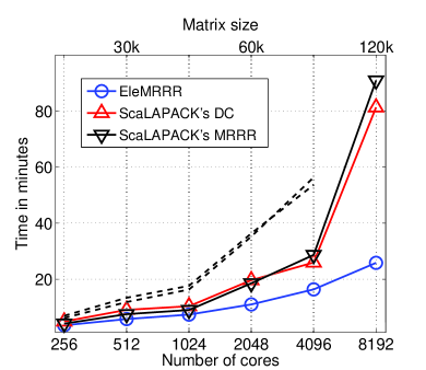
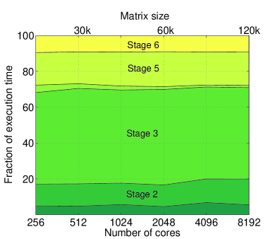
Both graphs show a similar behavior to the experiments performed on Juropa. In all experiments EleMRRR outperforms both of the ScaLAPACK’s solvers. Most importantly, ScaLAPACK again suffers from a breakdown in scalability.

When analyzing the results of Fig. E.1 for ScaLAPACK’s solver we the following three observations: (1) The scalability issues can be attributed mainly to Stages 1, 2, and 4. In particular, for the largest experiment ScaLAPACK’s reduction to standard form (28 minutes) and MRRR (25 minutes) each exceed the time that EleMRRR spends for the entire problem. (2) Although ScaLAPACK’s tridiagonal eigensolver is usually not very time consuming, for highly parallel systems it might become the bottleneck. As an example, in our experiment on 8,192 cores the tridiagonal problem accounts for 54% (MRRR) and 33% (DC) of the total execution time of the standard eigenproblem. (3) Due to better scalability, DC becomes faster than ScaLAPACK’s MRRR.

We conclude with four comments regarding EleMRRR’s behavior: (1) While stage 4 of ScaLAPACK’s MRRR and DC take up to 28% and 20% of the total execution time, respectively, PMRRR accounts for less than 4%. In particular, for the largest problem 25 minutes were spent in ScaLAPACK’s MRRR, whereas PMRRR required only 20 seconds. In all experiments PMRRR’s execution time was negligible. (2) The timings corresponding to the standard eigenproblem account for 70%–74% of the generalized problem’s execution time. (3) The part which is roughly proportional to the fraction of desired eigenpairs makes up 26%–32% of both the generalized and standard problem. (4) All of the six stages scale equally well and no computational bottleneck emerges.

Appendix F First Tests of Mixed Precision MRRR

In this section, we report on the first performance and accuracy results that we obtained for the mixed precision MRRR. All experiments were performed sequentially on Westmere. For the mixed precision results, we used the same reduction and backtransformation routines as LAPACK. For the extended precision results, we used version 4.7 of the GNU compilers.

Since for single precision input/output the mixed precision MRRR usually is faster than the conventional MRRR, we concentrate on double precision input/output. In this case, the mixed precision approach uses either extended or quadruple precision. We refer to these cases as mr3smp-extended and mr3smp-quad, respectively. The use of quadruple is more critical as it shows that the approach is applicable in many circumstances, even when the higher precision arithmetic used in the tridiagonal stage is much slower than arithmetic in the input/output format.

We confine ourselves to experiments on a small set of application matrices as listed in Table F.1, coming from quantum chemistry and structural mechanics problems. As the performance depends on the spectra of the input matrices, the platform of the experiment, and the implementation of the quadruple arithmetic, we cannot draw final conclusions from these limited test. However, the orthogonality improvements are quite general and are observed for a much larger test set originating from [104]. We do not report on residuals as the largest residual norms are generally comparable for all solvers.

Matrix	Size	Application	Reference
$A$	$2{,}053$	Chemistry	ZSM-5 in [56] and Fann3 in [104]
$B$	$4{,}289$	Chemistry	Originating from [21]
$C$	$4{,}704$	Mechanics	T_nasa4704 in [104]
$D$	$7{,}923$	Mechanics	See [13] for information
$E$	$12{,}387$	Mechanics	See [13] for information
$F$	$13{,}786$	Mechanics	See [13] for information
$G$	$16{,}023$	Mechanics	See [13] for information

Table F.1: A set of test matrices.

To better display the effects of the use of mixed precisions, the performance results are simplified in the following sense: As the routines for the reduction to tridiagonal form and the backtransformation of all solvers are the same, we used for these stages the minimum execution time of all runs for all solvers. In this way, the cost of the mixed precision approach becomes more visible and we do not have to resort to statistical metrics for the timings. We point out that especially for the subset tests, the run time of the tridiagonal stage for larger matrices is often smaller than the fluctuations in the timings for the reduction to tridiagonal form.

F.1 Real symmetric matrices

Computing all eigenpairs.

Figure F.1 refers to the computation of all eigenpairs. We report on the execution time of the mixed precision routines relative to LAPACK’s MRRR (DSYEVR) and the obtained orthogonality. As a reference, results for LAPACK’s DC (DSYEVD) are included. The orthogonality is improved using extended and quadruple precision. The left plot shows the performance penalty that we pay for the improvements. In particular, for larger matrices, the additional cost of the mixed precision approach becomes negligible, making it extremely attractive for large-scale problems. For example, for test matrices $E$, $F$, and $G$, our solver mr3smp-quad is as fast as DSYEVD, although it uses software-simulated arithmetic, while achieving better orthogonality. Since the quadruple arithmetic is currently much slower than the double one, mr3smp-quad carries a performance penalty for small matrices. In our case, for matrices with $n<2{,000}$, one must expect an increase in the total execution time of a factor larger than two. The situation is similar to the one reported in [10] for the mixed precision iterative refinement of the solution of linear systems of equations, where the mixed precision approach comes with a performance penalty for small matrices.

Figure F.1: Computation of all eigenpairs. Left: Execution time relative to routine DSYEVR. Right: Orthogonality.

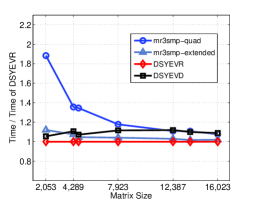
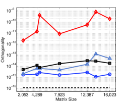
In contrast to mr3smp-quad, the use of extended precision does not significantly increase the execution time even for smaller matrices, while still improving the orthogonality. As the reason for different performance is solely due to the tridiagonal eigensolver, in the left panel of Fig. F.2 we show the execution time of the tridiagonal eigensolvers relative to LAPACK’s MRRR (DSTEMR).

Figure F.2: Execution time of the tridiagonal stage relative to LAPACK’s MRRR. Left: Computation of all eigenpairs. Right: Computation of 20% of the eigenpairs corresponding to the smallest eigenvalues.

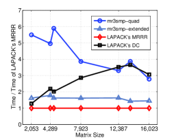
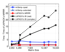
We remark that, although the mixed precision approach slows down the tridiagonal stage compared to DSTEMR (at least with the current support for quadruple precision arithmetic, see Fig. F.2), it has two features compensating this disadvantage: the approach increases robustness and parallel scalability of the code. To underpin these statements, in Table F.2, for the computation of all eigenpairs, we present the recursion depth $d_{max}$, the maximal cluster size and the number of times Line 16 in Algorithm 2 (the only possible source of failure) is executed.

		$A$	$B$	$C$	$D$	$E$	$F$	$G$
max. depth	DSTEMR	$2$	$2$	$2$	$4$	$5$	$2$	$5$
	mr3smp-quad	$0$	$0$	$0$	$0$	$0$	$0$	$0$
largest cluster	DSTEMR	$324$	$1{,}027$	$10$	$5{,}011$	$8{,}871$	$1{,}369$	$14{,}647$
	mr3smp-quad	$1$	$1$	$1$	$1$	$1$	$1$	$1$
new RRR	DSTEMR	$311$	$638$	$1{,}043$	$1{,}089$	$1{,}487$	$1{,}798$	$1{,}825$
	mr3smp-quad	$0$	$0$	$0$	$0$	$0$	$0$	$0$

Table F.2: Recursion depth, largest encountered cluster, and number of times an RRR for a cluster needs to be computed by executing Line 16 in Algorithm 2 for DSTEMR and mr3smp-quad.

In all cases, mr3smp-quad computes the eigenpairs directly from the root representation. Since this representation can be made definite, no danger of element growth in its computation exist (thus, the RRR can be found). Such a danger occurs in Line 16, where a new RRR for each cluster needs to be computed. By executing Line 16 only a few times – often no times at all – the danger of not finding a proper RRR is reduced and robustness increased. Since our approach is independent of the actual form of the RRRs, it is possible to additionally use twisted or blocked factorizations as proposed in [178, 176].

The mixed precision MRRR is especially appealing in the context of distributed-memory systems. The fact that all eigenpairs in our experiment are computed directly from the root representation implies that the execution is truly embarrassingly parallel. That MRRR is embarrassingly parallel was already announced – somewhat prematurely – with its introduction [40]. Only later, parallel versions of MRRR [13, 162] found that “the eigenvector computation in MRRR is only embarrassingly parallel if the root representation consists of singletons” [161] and that otherwise “load imbalance can occur and hamper the overall performance” [162].

While one can expect limited clustering of eigenvalues for application matrices arising from dense inputs, it is not always the case that the recursion depth is zero. Experiments on all the tridiagonal matrices provided explicitly by the Stetester [104] – a total of 176 matrices ranging in size from 3 to 24,873 – showed that the largest residual norm and worst case orthogonality were given by respectively $1.5\cdot 10^{-14}$ and $1.2\cdot 10^{-15}$ and $d_{max}\leq 2$. In fact, only four artificially constructed matrices, glued Wilkinson matrices [45], had clusters within clusters. In most cases, with the settings of our experiments, the clustering was very benign or even no clustering was observed. For example, the largest matrix in the test set, Bennighof_24873, had only a single cluster of size 37. Furthermore, it is also possible to significantly lower the $gaptol$ parameter, say to $10^{-16}$, and reduce clustering even more. For such small values of $gaptol$, in the approximation and refinement of eigenvalues we need to resort to quadruple precision, which so far we avoided for performance reasons, see Chapter 5.

Our results suggest that even better results can be expected for parallel executions. The MRRR algorithm was already reasonably scalable, and the mixed precision approach additionally improves scalability – often making the computation truly embarrassingly parallel.

Computing a subset of eigenpairs.

The situation is more favorable when only a subset of eigenpairs needs to be computed. As DSYEVD does not allow subset computations at reduced cost, a user can resort to either BI or MRRR. The capabilities of BI are accessible via LAPACK’s routine DSYEVX. Recently, the routine DSYEVR was edited, so that it uses BI instead of MRRR in the subset case. We therefore refer to ’DSYEVR (BI)’ when we use BI and ’DSYEVR (MRRR)’ when we force the use of MRRR instead. In Fig. F.3, we report the execution time relative to LAPACK’s MRRR for computing 20% of the eigenpairs associated with the smallest eigenvalues and the corresponding orthogonality.

Figure F.3: Computation of 20% of the eigenpairs corresponding to the smallest eigenvalues. Left: Execution time relative to routine DSYEVR that is forced to use MRRR. Right: Orthogonality.

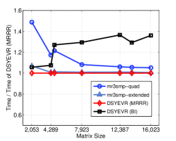
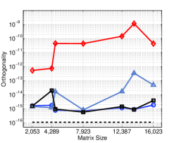
BI and mr3smp-quad achieved the best orthogonality. At the moment, for small matrices ($n\ll 2{,}000$), the use quadruple might be be too expensive. In this case, the mixed precision routine can easily be run in double precision only or BI can be used for accuracy and performance. As support for quadruple precision improves, the overhead will further decrease or completely vanish. The use of extended precision comes almost without any performance penalty. Unfortunately, for larger matrices, the orthogonality might still be inferior to other methods and no increased robustness and parallelism is observed. To illustrate the source of the differing run times, the right panel of Fig. F.2 presents the execution time of the tridiagonal eigensolver relative to LAPACK’s MRRR. As expected, due to explicit orthogonalization via the Gram-Schmidt procedure, BI potentially becomes considerably slower than MRRR.

F.2 Complex Hermitian matrices

Computing all eigenpairs.

In Fig. F.4, we show results for computing all eigenpairs. The left and right panel display the execution time of all solvers relative to LAPACK’s MRRR (ZHEEVR) and the orthogonality, respectively. As predicted, the extra cost due to the higher precision becomes relatively smaller for complex-valued input compared to real-valued input – compare Figs. F.1 and F.4. Similarly, if the mixed precision solver is used for the generalized eigenproblem based on Cholesky-Wilkinson algorithm (see Section 2.3.3), the approach increases the execution only marginally even for relatively small problems.

Figure F.4: Computation of all eigenpairs. Left: Execution time relative to routine ZHEEVR. Right: Orthogonality.

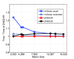
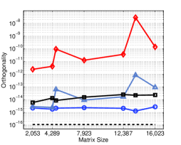
We remark that the timing plots might be misleading and suggest that the cost of the mixed precision approach is high. Indeed, for test matrix $A$, using quadruple precision increased the run time by about 23% relative to ZHEEVR. This means in absolute time that the mixed precision approach required about 27 seconds and ZHEEVR only 22 seconds. For larger matrices the absolute execution time increases as $n^{3}$ and the performance gap between mixed precision approach and pure double precision solver vanishes. Such a scenario is observed with test matrix $F$, for which we obtain an orthogonality of $1.3\cdot 10^{-15}$ with mr3smp-quad compared to $2.9\cdot 10^{-8}$ with ZHEEVR, while spending only about 4% more in the total execution time.

Computing a subset of eigenpairs.

We compute 20% of the eigenpairs associated with the smallest eigenvalues. The execution time relative to LAPACK’s MRRR and the corresponding orthogonality are displayed in Fig. F.5.

Figure F.5: Computation of 20% of the eigenpairs corresponding to the smallest eigenvalues are computed. Left: Execution time relative to routine ZHEEVR (when forced to use MRRR). Right: Orthogonality.

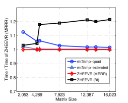
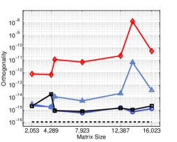
The extra cost due to the use of higher precision in mr3smp-extended or mr3smp-quad were quite small. Even using quadruple precision, the run time only increased by maximally 13%. In a similar experiment – computing 10% of the eigenpairs corresponding to the smallest eigenvalues – the extra cost for mr3smp-quad was less than 6% compared to LAPACK’s MRRR. Such a penalty in the execution time is already below the fluctuations observed in repeated experiments. While mr3smp-extended is faster than mr3smp-quad for smaller problems, it cannot quite deliver the same orthogonality.

The relative timings of the tridiagonal eigensolvers are depicted in the right panel of Fig. F.2. Interestingly, BI is almost by a factor two slower than in the real-valued case. The reason is that the Gram-Schmidt orthogonalization, a memory bandwidth-limited operation, is performed on complex data (although all imaginary parts of the involved vectors are zero).

F.3 Summary

The mixed precision MRRR obtains much improved orthogonality – possibly at the cost of some performance. The performance penalty depends on the difference in speed between the precision of input/output and the higher precision used in the tridiagonal stage. In the single/double case, the mixed precision approach does not introduce a penalty and usually leads faster executions; in the double/quadruple case, the mixed precision approach does introduce a penalty for small matrices. For larger matrices, the additional cost becomes negligible as the tridiagonal stage has a lower complexity than the other two stages of the standard Hermitian eigenproblem. In the future, with improved support for quadruple – through (partial) hardware support or advances in the algorithms for software simulation – the additional cost of the mixed precision approach vanishes. The use of a hardware supported 80-bit extended floating point format provides an alternative. In this case, the execution time is hardly affected, but it cannot guarantee the same orthogonality. In addition to improving the orthogonality, our approach increases both robustness and scalability of the solver. For this reasons, the mixed precision approach is ideal for large-scale distributed-memory solvers.

Appendix G Mixed Precision MRRR on Application Matrices

We use test set Application, detailed in Appendix D, to augment our previous results for test set Artificial. Most Application matrices are part of the publicly available Stetester suite [104] and range from $1{,}074$ to $8{,}012$ in size.

In Figs. G.1 and G.2, we present accuracy and timings for the single precision matrices in tridiagonal form.

(a) Execution time: sequential.

(b) Execution time: multi-threaded.

Figure G.1: Timings for test set Application on Beckton. The single precision input matrices $T\in\mathbb{R}^{n\times n}$ are tridiagonal.

(a) Largest residual norm.

(b) Orthogonality.

Figure G.2: Accuracy for test set Application. The single precision input matrices $T\in\mathbb{R}^{n\times n}$ are tridiagonal.

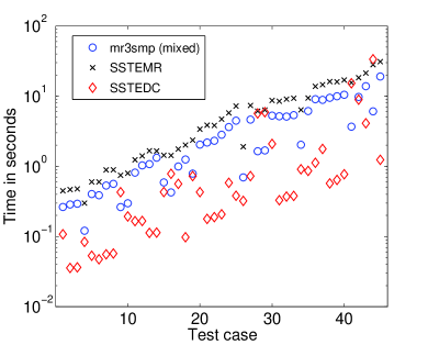
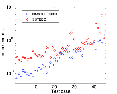
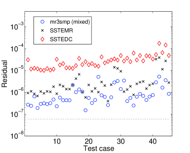
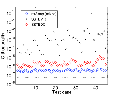
The tests correspond to Figs. 5.4 and 5.5 in Section 5.3. As matrices are quite small for the resources, we hardly see any speedup through multi-threading for the smallest matrices. Nonetheless, the mixed precision MRRR is highly competitive with DC, both in terms of performance and accuracy.

Corresponding to Figs. 5.7 and 5.8 in Section 5.3, we performed the experiment on test set Application in double precision. The results are presented in Figs. G.3 and G.4.

(a) Execution time: sequential.

(b) Execution time: multi-threaded.

Figure G.3: Timings for test set Application on Beckton. The double precision input matrices $T\in\mathbb{R}^{n\times n}$ are tridiagonal.

(a) Largest residual norm.

(b) Orthogonality.

Figure G.4: Accuracy for test set Application. The double precision input matrices $T\in\mathbb{R}^{n\times n}$ are tridiagonal.

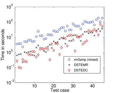
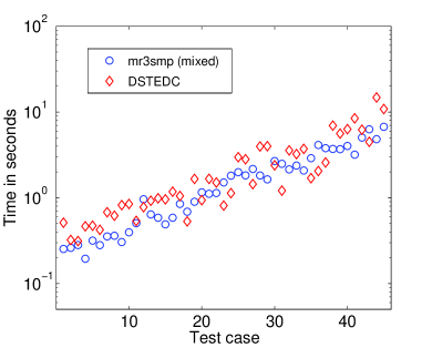
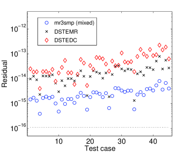
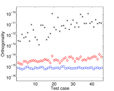
In sequential executions, as the matrices are smaller than for test set Artificial and we use a rather slow software-simulated quadruple precision arithmetic, the mixed precision solver is considerably slower than both DSTEDC and DSTEMR. Such a performance penalty vanishes for parallel executions.

Robustness, measured by $\phi(\mbox{\sc Application})$, is increased: while for DSTEMR $\phi\approx 0.02$, we have $\phi\approx 0.71$ for the mixed precision MRRR, even without taking the relaxed requirements of (5.6) and (5.7) into account. By only very conservatively relaxing the requirements on what constitutes an RRR, we already achieve $\phi\approx 0.98$; for all matrices, only a single representation is accepted without passing the test for being an RRR. We suspect that, by properly adjusting the test for relative robustness, we can easily achieve $\phi(\mbox{\sc Application})=1$ and thereby guarantee accuracy for all inputs. These numbers support our believe that the use of mixed precisions might be an important ingredient for MRRR to achieve robustness comparable to the most reliable solvers.

Similar to Fig. 5.6 in Section 5.3, we show in Fig. G.5 the maximal depth of the representation tree, $d_{max}$.

(a) Single precision.

(b) Double precision.

Figure G.5: Maximal depth of the representation tree, $d_{max}$.

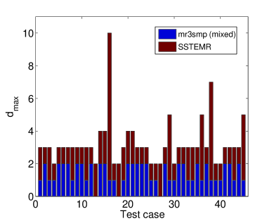
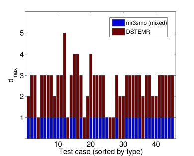
In contrast to test set Artificial, $d_{max}$ is limited to small values for both SSTEMR and DSTEMR; the Application matrices are smaller and have less clustering of eigenvalues. For the mixed precision MRRR, $d_{max}$ is limited to two in the single/double case and to one in the double/quadruple case.

For single precision symmetric dense inputs $A\in\mathbb{R}^{n\times n}$, we show results in Figs. G.6 and G.7.

(a) Execution time: sequential.

(b) Execution time: multi-threaded.

Figure G.6: Timings for test set Application on Beckton. The single precision input matrices $A\in\mathbb{R}^{n\times n}$ are dense.

(a) Largest residual norm.

(b) Orthogonality.

Figure G.7: Accuracy for test set Application. The single precision input matrices $A\in\mathbb{R}^{n\times n}$ are dense.

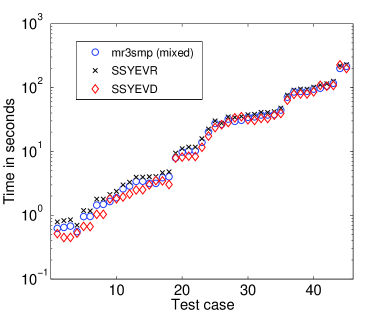
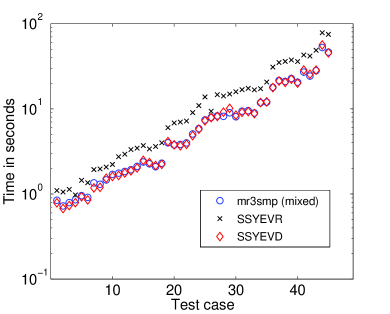
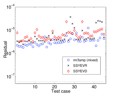
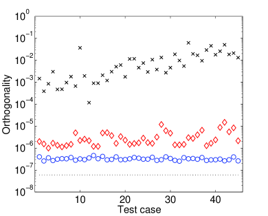
The experiment corresponds to Figs. 5.9 and 5.10 in Section 5.3. The matrices are generated by applying random orthogonal similarity transformations to the tridiagonal matrices of the previous experiments: $A=QTQ^{*}$, with random orthogonal matrix $Q\in\mathbb{R}^{n\times n}$. The execution time is dominated by the reduction to tridiagonal form and the backtransformation of the eigenvectors. As the first stage, SSYTRD, does not scale well, so does the overall problem. Similar results are also obtained for executions with a smaller number of threads.

For double precision real symmetric dense inputs $A\in\mathbb{R}^{n\times n}$, we show results in Figs. G.8 and G.9. The experiment corresponds to Figs. 5.11 and 5.12 in Section 5.3.

(a) Execution time: sequential.

(b) Execution time: multi-threaded.

Figure G.8: Timings for test set Application on Beckton. The double precision input matrices $A\in\mathbb{R}^{n\times n}$ are dense.

(a) Largest residual norm.

(b) Orthogonality.

Figure G.9: Accuracy for test set Application. The double precision input matrices $A\in\mathbb{R}^{n\times n}$ are dense.

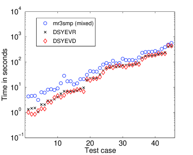
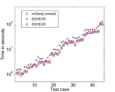
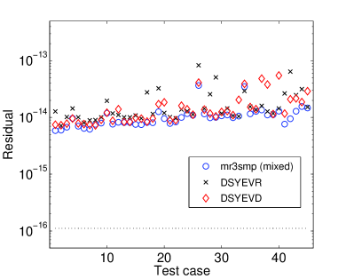
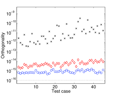
For small matrices, the sequential execution is slower than DSYEVR, but the performance gap reduces as the matrix size increases. The accuracy improvements are limited to the orthogonality; the residuals are often comparable for all solvers. If input matrices become complex-valued and/or only a subset of eigenpairs needs to be computed, a possible overhead due to the use of mixed precisions is reduced as the reduction to tridiagonal form would carry even more weight relative to the tridiagonal stage.

References

- [1] Å. Björck. Numerics of Gram-Schmidt orthogonalization. Linear Algebra and its Applications 197–198, 0 (1994), 297 – 316.
- [2] Agullo, E., Demmel, J., Dongarra, J., Hadri, B., Kurzak, J., Langou, J., Ltaief, H., Luszczek, P., and Tomov, S. Numerical Linear Algebra on Emerging Architectures: The PLASMA and MAGMA Projects. Journal of Physics: Conference Series 180 (2009).
- [3] Aliaga, J., Bientinesi, P., Davidovic, D., Di Napoli, E., Igual, F., and Quintana-Ortí, E. Solving Dense Generalized Eigenproblems on Multi-Threaded Architectures. Applied Mathematics and Computation 218, 22 (2012), 11279–11289.
- [4] Amdahl, G. M. Validity of the single processor approach to achieving large scale computing capabilities. In Proceedings of the April 18-20, 1967, spring joint computer conference (New York, NY, USA, 1967), AFIPS ’67 (Spring), ACM, pp. 483–485.
- [5] Anderson, E., Bai, Z., Bischof, C., Blackford, S., Demmel, J., Dongarra, J., Croz, J. D., Greenbaum, A., Hammarling, S., McKenney, A., and Sorensen, D. LAPACK Users’ Guide, third ed. SIAM, Philadelphia, PA, 1999.
- [6] Arbenz, P. Divide and conquer algorithms for the bandsymmetric eigenvalue problem. Parallel Computing 18, 10 (1992), 1105 – 1128.
- [7] Asanovic, K., Bodik, R., Catanzaro, B. C., Gebis, J. J., Husbands, P., Keutzer, K., Patterson, D. A., Plishker, W. L., Shalf, J., Williams, S. W., and Yelick, K. A. The Landscape of Parallel Computing Research: A View from Berkeley. Tech. Rep. UCB/EECS-2006-183, EECS Department, University of California, Berkeley, 2006.
- [8] Auckenthaler, T., Blum, V., Bungartz, H.-J., Huckle, T., Johanni, R., Krämer, L., Lang, B., Lederer, H., and Willems, P. Parallel Solution of Partial Symmetric Eigenvalue Problems from Electronic Structure Calculations. Parallel Comput. 37 (2011), 783–794.
- [9] Auckenthaler, T., Bungartz, H.-J., Huckle, T., Kraemer, L., Lang, B., and Willems, P. Developing algorithms and software for the parallel solution of the symmetric eigenvalue problem. Journal of Computational Science 2, 3 (2011), 272 – 278.
- [10] Baboulin, M., Buttari, A., Dongarra, J., Kurzak, J., Langou, J., Langou, J., Luszczek, P., and Tomov, S. Accelerating Scientific Computations with Mixed Precision Algorithms. Computer Physics Communications 180, 12 (2009), 2526 – 2533.
- [11] Ballard, G., Demmel, J., and Knight, N. Communication avoiding successive band reduction. SIGPLAN Not. 47, 8 (2012), 35–44.
- [12] Barth, W., Martin, R. S., and Wilkinson, J. H. Calculation of the Eigenvalues of a Symmetric Tridiagonal Matrix by the Method of Bisection. Numer. Math. V9, 5 (1967), 386–393.
- [13] Bientinesi, P., Dhillon, I., and van de Geijn, R. A Parallel Eigensolver for Dense Symmetric Matrices Based on Multiple Relatively Robust Representations. SIAM J. Sci. Comput. 27 (2005), 43–66.
- [14] Bientinesi, P., Igual, F. D., Kressner, D., Petschow, M., and Quintana-Ortí, E. S. Condensed forms for the symmetric eigenvalue problem on multi-threaded architectures. Concurrency and Computation: Practice and Experience 23, 7 (2011), 694–707.
- [15] Bischof, C., Huss-Lederman, S., Sun, X., and Tsao, A. The PRISM project: infrastructure and algorithms for parallel eigensolvers. In Proceedings of the Scalable Parallel Libraries Conference (1993), pp. 123 –131.
- [16] Bischof, C., Huss-Lederman, S., Sun, X., Tsao, A., and Turnbull, T. Parallel performance of a symmetric eigensolver based on the invariant subspace decomposition approach. In Proceedings of the Scalable High-Performance Computing Conference (1994), pp. 32 –39.
- [17] Bischof, C., Lang, B., and Sun, X. Parallel tridiagonalization through two-step band reduction. In In Proceedings of the Scalable High-Performance Computing Conference (1994), IEEE Computer Society Press, pp. 23–27.
- [18] Bischof, C., Lang, B., and Sun, X. A Framework for Symmetric Band Reduction. ACM Trans. Math. Software 26 (2000), 581–601.
- [19] Bischof, C. H., Lang, B., and Sun, X. Algorithm 807: The SBR toolbox-software for successive band reduction. ACM Trans. Math. Software 26, 4 (2000), 602–616.
- [20] Blackford, L. S., Choi, J., Cleary, A., D’Azevedo, E., Demmel, J., Dhillon, I., Dongarra, J., Hammarling, S., Henry, G., Petitet, A., Stanley, K., Walker, D., and Whaley, R. C. ScaLAPACK Users’ Guide. SIAM, Philadelphia, PA, USA, 1997.
- [21] Blügel, S., Bihlmeyer, G., Wortmann, D., Friedrich, C., Heide, M., Lezaic, M., Freimuth, F., and Betzinger, M. The Jülich FLEUR Project. Jülich Research Center, 1987. http://www.flapw.de.
- [22] Bowdler, H., Martin, R., Reinsch, C., and Wilkinson, J. The and algorithms for symmetric matrices. Numerische Mathematik 11 (1968), 293–306.
- [23] Chan, E., Van Zee, F. G., Bientinesi, P., Quintana-Ortí, E. S., Quintana-Ortí, G., and van de Geijn, R. Supermatrix: a multithreaded runtime scheduling system for algorithms-by-blocks. In Proceedings of the 13th ACM SIGPLAN Symposium on Principles and practice of parallel programming (New York, NY, USA, 2008), PPoPP ’08, ACM, pp. 123–132.
- [24] Chandrasekaran, S. An Efficient and Stable Algorithm for the Symmetric-Definite Generalized Eigenvalue Problem. SIAM J. Matrix Anal. Appl. 21, 4 (2000), 1202–1228.
- [25] Chang, H., Utku, S., Salama, M., and Rapp, D. A parallel householder tridiagonalization stratagem using scattered square decomposition. Parallel Computing 6, 3 (1988), 297 – 311.
- [26] Choi, J., Demmel, J., Dhillon, I., Dongarra, J., Ostrouchov, S., Petitet, A., Stanley, K., Walker, D., and Whaley, R. C. ScaLAPACK: a Portable Linear Algebra Library for Distributed Memory Computers – Design Issues and Performance. Computer Physics Communications 97, 1-2 (1996), 1 – 15. High-Performance Computing in Science.
- [27] Chtchelkanova, A., Gunnels, J., Morrow, G., Overfelt, J., and van de Geijn, R. Parallel implementation of blas: General techniques for level 3 blas. Tech. rep., Austin, TX, USA, 1995.
- [28] Crawford, C. R. Reduction of a band-symmetric generalized eigenvalue problem. Commun. ACM 16, 1 (1973), 41–44.
- [29] Cuppen, J. A Divide and Conquer Method for the Symmetric Tridiagonal Eigenproblem. Numer. Math. 36 (1981), 177–195.
- [30] Dai, G.-L., Liu, Z.-P., Wang, W.-N., Lu, J., and Fan, K.-N. Oxidative Dehydrogenation of Ethane over V2O5 (001): A Periodic Density Functional Theory Study. J. Phys. Chem. C 112 (2008), 3719–3725.
- [31] Davis, C., and Kahan, W. The Rotation of Eigenvectors by a Perturbation. III. SIAM J. Numer. Anal. 7, 1 (1970), pp. 1–46.
- [32] Demmel, J. Applied Numerical Linear Algebra. SIAM, Philadelphia, PA, USA, 1997.
- [33] Demmel, J., Dhillon, I., and Ren, H. On the Correctness of some Bisection-like Parallel Eigenvalue Algorithms in Floating Point Arithmetic. Electronic Trans. Num. Anal. 3 (1995), 116–149.
- [34] Demmel, J., Dongarra, J., Ruhe, A., and van der Vorst, H. Templates for the Solution of Algebraic Eigenvalue Problems: a Practical Guide. SIAM, Philadelphia, PA, USA, 2000.
- [35] Demmel, J., Heath, M. T., and van der Vorst, H. A. Parallel numerical linear algebra. Acta Numerica 2 (1993), 111–197.
- [36] Demmel, J., and Kahan, W. Accurate singular values of bidiagonal matrices. SIAM J. SCI. STAT. COMPUT 11, 5 (1990), 873–912.
- [37] Demmel, J., Marques, O., Parlett, B., and Vömel, C. Performance and Accuracy of LAPACK’s Symmetric Tridiagonal Eigensolvers. SIAM J. Sci. Comp. 30 (2008), 1508–1526.
- [38] Demmel, J., and Stanley, K. The Performance of Finding Eigenvalues and Eigenvectors of Dense Symmetric Matrices on Distributed Memory Computers. Tech. Rep. CS-94-254, University of Tennessee, Knoxville, TN, USA, 1994. LAPACK Working Note 86.
- [39] Demmel, J., and Veselic, K. Jacobi’s Method is more accurate than QR. SIAM J. Matrix Anal. Appl 13 (1992), 1204–1245.
- [40] Dhillon, I. A New Algorithm for the Symmetric Tridiagonal Eigenvalue/Eigenvector Problem. PhD thesis, EECS Department, University of California, Berkeley, 1997.
- [41] Dhillon, I. Current Inverse Iteration Software Can Fail. BIT 38 (1998), 685–704.
- [42] Dhillon, I., Fann, G., and Parlett, B. Application of a New Algorithm for the Symmetric Eigenproblem to Computational Quantum Chemistry. In Proceedings of the Eighth SIAM Conference on Parallel Processing for Scientific Computing (Minneapolis, MN, 1997), SIAM.
- [43] Dhillon, I., and Parlett, B. Multiple Representations to Compute Orthogonal Eigenvectors of Symmetric Tridiagonal Matrices. Linear Algebra Appl. 387 (2004), 1–28.
- [44] Dhillon, I., and Parlett, B. Orthogonal Eigenvectors and Relative Gaps. SIAM J. Matrix Anal. Appl. 25 (2004), 858–899.
- [45] Dhillon, I., Parlett, B., and Vömel, C. Glued Matrices and the MRRR Algorithm. SIAM J. Sci. Comput. 27, 2 (2005), 496–510.
- [46] Dhillon, I., Parlett, B., and Vömel, C. The Design and Implementation of the MRRR Algorithm. ACM Trans. Math. Software 32 (2006), 533–560.
- [47] Domas, S., and Tisseur, F. Parallel implementation of a symmetric eigensolver based on the yau and lu method. In Selected papers from the Second International Conference on Vector and Parallel Processing (London, UK, UK, 1997), VECPAR ’96, Springer-Verlag, pp. 140–153.
- [48] Dongarra, J. Freely available software for linear algebra. http://www.netlib.org/utk/people/JackDongarra/la-sw.html, Sept. 2011.
- [49] Dongarra, J., Du Croz, J., Hammarling, S., and Hanson, R. J. An extended set of fortran basic linear algebra subprograms. ACM Trans. Math. Software 14, 1 (1988), 1–17.
- [50] Dongarra, J., Du Cruz, J., Duff, I., and Hammarling, S. A Set of Level 3 Basic Linear Algebra Subprograms. ACM Trans. Math. Software 16 (1990), 1–17.
- [51] Dongarra, J., and Sorensen, D. A fully parallel algorithm for the symmetric eigenvalue problem. SIAM J. Sci. Stat. Comput. 8, 2 (1987), 139–154.
- [52] Dongarra, J., Sorensen, D. C., and Hammarling, S. J. Block reduction of matrices to condensed forms for eigenvalue computations. J. Comput. Appl. Math 27 (1989), 215–227.
- [53] Dongarra, J., and van de Geijn, R. A. Reduction to condensed form for the eigenvalue problem on distributed memory architectures. Parallel Computing 18, 9 (1992), 973–982.
- [54] Elwood, D., Fann, G., and Littlefield, R. PeIGS User’s Manual. Pacific Northwest National Laboratory, WA, 1993.
- [55] Fang, H., and O’Leary, D. Stable factorizations of symmetric tridiagonal and triadic matrices. SIAM J. Matrix Anal. Appl. 28 (2006), 576–595.
- [56] Fann, G., Littlefield, R., and Elwood, D. Performance of a Fully Parallel Dense Real Symmetric Eigensolver in Quantum Chemistry Applications. In Proceedings of High Performance Computing ’95 (1995), Simulation MultiConference, The Society for Computer Simulation.
- [57] Fernando, K. Accurate BABE Factorisation of Tridiagonal Matrices for Eigenproblems. Tech. rep., NAG Ltd., TR5/95, 1995.
- [58] Fernando, K. On a classical method for computing eigenvectors. Tech. rep., NAG Ltd., TR3/95, 1995.
- [59] Fernando, K. On computing an eigenvector of a tridiagonal matrix. Tech. rep., NAG Ltd., TR4/95, 1995.
- [60] Fernando, K. V., and Parlett, B. Accurate singular values and differential qd algorithms. Numerische Mathematik 67 (1994), 191–229.
- [61] Francis, J. The QR Transform - A Unitary Analogue to the LR Transformation, Part I and II. The Comp. J. 4 (1961/1962).
- [62] Gansterer, W. N., Schneid, J., and Ueberhuber, C. W. A Divide-and-Conquer Method for Symmetric Banded Eigenproblems - Part I: Theoretical Results. Tech. Rep. AURORA TR1999-12, Vienna University of Technology, 1998.
- [63] Gansterer, W. N., Schneid, J., and Ueberhuber, C. W. A Divide-and-Conquer Method for Symmetric Banded Eigenproblems - Part II: Algorithmic Aspects. Tech. Rep. AURORA TR1999-14, Vienna University of Technology, 1998.
- [64] Givens, W. Numerical computation of the characteristic values of a real matrix. Technical Report 1574, Oak Ridge National Laboratory, Oak Ridge, TN, 1954.
- [65] Godunov, S., Kostin, V., and Mitchenko, A. Computation of an eigenvector of a symmetric tridiagonal matrix. Siberian Mathematical Journal 26 (1985), 684–696.
- [66] Golub, G. H., and Loan, C. F. V. Matrix Computations, 3rd ed. The Johns Hopkins University Press, 1996.
- [67] Gu, M., and Eisenstat, S. C. A stable and efficient algorithm for the rank-one modification of the symmetric eigenproblem. SIAM J. Matrix Anal. Appl. 15, 4 (1994), 1266–1276.
- [68] Gu, M., and Eisenstat, S. C. A Divide-and-Conquer Algorithm for the Symmetric Tridiagonal Eigenproblem. SIAM J. Matrix Anal. Appl. 16, 1 (1995), 172–191.
- [69] Gustafson, J. L. Reevaluating Amdahl’s Law. Comm. ACM 31, 5 (1988), 532–533.
- [70] Haidar, A., Ltaief, H., and Dongarra, J. Parallel reduction to condensed forms for symmetric eigenvalue problems using aggregated fine-grained and memory-aware kernels. In Proceedings of 2011 International Conference for High Performance Computing, Networking, Storage and Analysis (New York, NY, USA, 2011), SC ’11, pp. 8:1–8:11.
- [71] Haidar, A., Ltaief, H., and Dongarra, J. Toward a high performance tile divide and conquer algorithm for the dense symmetric eigenvalue problem. SIAM Journal on Scientific Computing 34, 6 (2012), C249–C274.
- [72] Hendrickson, B., Jessup, E., and Smith, C. Toward an Efficient Parallel Eigensolver for Dense Symmetric Matrices. SIAM J. Sci. Comput. 20 (1999), 1132–1154.
- [73] Hendrickson, B. A., and Womble, D. E. The Torus-Wrap Mapping For Dense Matrix Calculations On Massively Parallel Computers. SIAM J. Sci. Stat. Comput. 15 (1994), 1201–1226.
- [74] Herlihy, M., and Luchangco, V. Distributed computing and the multicore revolution. SIGACT News 39, 1 (2008), 62–72.
- [75] Hernández, V., Román, E., Tomás, and Vidal, V. A Survey of Software for Sparse Eigenvalue Problems. Tech. Rep. SLEPc Technical Report STR-6, Universidad Politechnica de Valencia, 2009.
- [76] Hiroyuki, I., Kinji, K., and Yoshimasa, N. Implementation and performance evaluation of new inverse iteration algorithm with householder transformation in terms of the compact representation. Tech. Rep. 8, Graduate school of Informatics, Kyoto University, 2011.
- [77] Hoffmann, W., and Parlett, B. A New Proof of Global Convergence for the Tridiagonal Algorithm. SIAM Journal on Numerical Analysis 15, 5 (1978), 929–937.
- [78] Hogben, L. Handbook of Linear Algebra. Discrete Mathematics And Its Applications. Taylor & Francis, 2006.
- [79] Horn, R. A., and Johnson, C. R. Matrix analysis. Cambridge University Press, Cambridge; New York, 1985.
- [80] Inaba, T., and Sato, F. Development of Parallel Density Functional Program using Distributed Matrix to Calculate All-Electron Canonical Wavefunction of Large Molecules. J. of Comp. Chemistry 28, 5 (2007), 984–995.
- [81] Ipsen, I. A history of inverse iteration. In Helmut Wielandt, Mathematische Werke, Mathematical Works, volume II: Matrix Theory and Analysis. Walter de Gruyter (1995).
- [82] Ipsen, I. Computing An Eigenvector With Inverse Iteration. SIAM Review 39 (1997), 254–291.
- [83] Jacobi, C. G. J. Über ein leichtes Verfahren die in der Theorie der Säcularstörungen vorkommenden Gleichungen numerisch aufzulösen. Crelle 30 (1846), 51–94.
- [84] Jessup, E. R., and Ipsen, I. Improving the accuracy of inverse iteration. SIAM J. Sci. Stat. Comput. 13, 2 (1992), 550–572.
- [85] Joffrain, T., Low, T. M., Quintana-Ortí, E. S., van de Geijn, R., and Van Zee, F. G. Accumulating Householder transformations, revisited. ACM Trans. Math. Softw. 32, 2 (2006), 169–179.
- [86] Kahan, W. Accurate eigenvalues of a symmetric tri-diagonal matrix. Tech. Rep. CS41, Stanford, CA, USA, 1966.
- [87] Kahan, W. When to neglect off-diagonal elements of symmetric tridiagonal matrices. Tech. Rep. CS42, Stanford, CA, USA, 1966.
- [88] Kent, P. Computational Challenges of Large-Scale Long-Time First-Principles Molecular Dynamics. J. Phys.: Conf. Ser. 125 (2008).
- [89] Kopp, J. Efficient numerical diagonalization of hermitian 3x3 matrices. Tech. Rep. arXiv:physics/0610206, 2006.
- [90] Kublanovskaya, V. On some Algorithms for the Solution of the Complete Eigenvalue Problem. Zh. Vych. Mat. 1 (1961), 555–572.
- [91] Lang, B. A parallel algorithm for reducing symmetric banded matrices to tridiagonal form. SIAM Journal on Scientific Computing 14, 6 (1993), 1320–1338.
- [92] Lang, B. Effiziente Orthogonaltransformationen bei der Eigen- und Singulärwertberechnung. Habilitationsschrift, Fachbereich Mathematik, Universität Wuppertal, 1997.
- [93] Lang, B. Using Level 3 BLAS in Rotation-Based Algorithms. SIAM J. Sci. Comput. 19, 2 (1998), 626–634.
- [94] Lang, B. Efficient eigenvalue and singular value computations on shared memory machines. Parallel Comput. 25, 7 (1999), 845–860.
- [95] Lang, B. Direct Solvers for Symmetric Eigenvalue Problems. In Modern Methods and Algorithms of Quantum Chemistry (2000), J. Grotendorst, Ed., NIC Series, Volume 3, pp. 231–259.
- [96] Lang, B. Out-of-core solution of large symmetric eigenproblems. Z. Angew. Math. Mech. 80 (2000), 809–810.
- [97] Lawson, C. L., Hanson, R. J., Kincaid, D. R., and Krogh, F. T. Basic Linear Algebra Subprograms for Fortran Usage. ACM Trans. Math. Software 5, 3 (1979), 308–323.
- [98] Li, R.-C. Solving Secular Equations Stably and Efficiently. Tech. Rep. UCB/CSD-94-260, Computer Science Dept., University of California, Berkeley, 1994.
- [99] Li, T., and Rhee, N. Homotopy algorithm for symmetric eigenvalue problems. Numerische Mathematik 55 (1989), 265–280.
- [100] Li, T. Y., and Zeng, Z. Laguerre’s iteration in solving the symmetric tridiagonal eigenproblem - revisited. SIAM J. Sci. Comput. 15 (1992), 1145–1173.
- [101] Luszczek, P., Ltaief, H., and Dongarra, J. Two-stage tridiagonal reduction for dense symmetric matrices using tile algorithms on multicore architectures. In Parallel Distributed Processing Symposium (IPDPS), 2011 IEEE International (2011), pp. 944 –955.
- [102] Marques, O., Parlett, B., and Vömel, C. Computations of Eigenpair Subsets with the MRRR Algorithm. Numerical Linear Algebra with Applications 13, 8 (2006), 643–653.
- [103] Marques, O., Riedy, E., and Vömel, C. Benefits of IEEE-754 Features in Modern Symmetric Tridiagonal Eigensolvers. SIAM J. Sci. Comput. 28 (2006), 1613–1633.
- [104] Marques, O. A., Vömel, C., Demmel, J., and Parlett, B. N. Algorithm 880: A Testing Infrastructure for Symmetric Tridiagonal Eigensolvers. ACM Trans. Math. Softw. 35, 1 (2008), 8:1–8:13.
- [105] Martin, R., Reinsch, C., and Wilkinson, J. The algorithm for band symmetric matrices. Numerische Mathematik 16 (1970), 85–92.
- [106] Martin, R., and Wilkinson, J. Reduction of the Symmetric Eigenproblem ; and Related Problems to Standard Form. Numerische Mathematik 11 (1968), 99–110.
- [107] Matsekh, A. M. The Godunov-inverse iteration: A fast and accurate solution to the symmetric tridiagonal eigenvalue problem. Appl. Numer. Math. 54, 2 (2005), 208–221.
- [108] Moler, C., and Stewart, G. An Algorithm for Generalized Matrix Eigenvalue Problems. SIAM J. on Numerical Analysis 10, 2 (1973), 241–256.
- [109] Nakatsukasa, Y., and Higham, N. Stable and Efficient Spectral Divide and Conquer Algorithms for the Symmetric Eigenvalue Decomposition and the SVD. Tech. Rep. No. 2012.52, Dept. of Mathematics, University of Manchester, 2012.
- [110] Oettli, M. H. A robust, parallel homotopy algorithm for the symmetric tridiagonal eigenproblem. SIAM J. Sci. Comput. 20, 3 (1999), 1016–1032.
- [111] Ortega, J. M., and Kaiser, H. F. The and methods for symmetric tridiagonal matrices. The Computer Journal 6, 1 (1963), 99–101.
- [112] Parlett, B. Construction of orthogonal eigenvectors for tight clusters by use of submatrices. Tech. Rep. CPAM-664, Center for Pure and Applied Mathematics, University of California, Berkeley, 1996.
- [113] Parlett, B. Invariant subspaces for tightly clustered eigenvalues of tridiagonals. BIT Numerical Mathematics 36 (1996), 542–562.
- [114] Parlett, B. The Symmetric Eigenvalue Problem. Prentice-Hall, Inc., Upper Saddle River, NJ, USA, 1998.
- [115] Parlett, B. For tridiagonals replace with . Journal of Computational and Applied Mathematics 123, 1–2 (2000), 117 – 130.
- [116] Parlett, B. The QR Algorithm. Comput. Sci. Eng. 2, 1 (2000), 38–42.
- [117] Parlett, B. Perturbation of Eigenpairs of Factored Symmetric Tridiagonal Matrices. Foundations of Computational Mathematics 3 (2003), 207–223.
- [118] Parlett, B., and Dhillon, I. Fernando’s Solution to Wilkinson’s Problem: an Application of Double Factorization. Linear Algebra Appl. 267 (1996), 247–279.
- [119] Parlett, B., and Dhillon, I. Relatively Robust Representations of Symmetric Tridiagonals. Linear Algebra Appl. 309, 1-3 (2000), 121 – 151.
- [120] Parlett, B., and Marques, O. An Implementation of the DQDS Algorithm (Positive Case). Linear Algebra Appl. 309 (1999), 217–259.
- [121] Peters, G., and Wilkinson, J. Inverse Iteration, Ill-Conditioned Equations and Newton’s Method. SIAM Review 21, 3 (1979), 339–360.
- [122] Petschow, M., and Bientinesi, P. The Algorithm of Multiple Relatively Robust Representations for Multi-Core Processors. K. Jonasson, Ed., vol. 7133 of Lecture Notes in Computer Science, Springer, pp. 152–161.
- [123] Petschow, M., and Bientinesi, P. MR3-SMP: A Symmetric Tridiagonal Eigensolver for Multi-Core Architectures. Parallel Computing 37, 12 (2011), 795 – 805.
- [124] Petschow, M., Peise, E., and Bientinesi, P. High-Performance Solvers For Dense Hermitian Eigenproblems. SIAM J. Sci. Comput. 35, 1 (2013), 1–22.
- [125] Petschow, M., Quintana-Ortí, E. S., and Bientinesi, P. Improved Orthogonality for Dense Hermitian Eigensolvers based on the MRRR algorithm. Tech. Rep. AICES-2012/09-1, RWTH Aachen, Germany, 2012.
- [126] Petschow, M., Quintana-Ortí, E. S., and Bientinesi, P. Improved Accuracy and Parallelism for MRRR-based Eigensolvers – A Mixed Precision Approach. SIAM J. Sci. Comput. (2014). Accpeted for publication.
- [127] Poulson, J., Marker, B., van de Geijn, R. A., Hammond, J. R., and Romero, N. A. Elemental: A New Framework for Distributed Memory Dense Matrix Computations. FLAME Working Note 44 (revised). Technical Report TR-10-20, The University of Texas at Austin, Department of Computer Sciences, 2011.
- [128] Poulson, J., Marker, B., van de Geijn, R. A., Hammond, J. R., and Romero, N. A. Elemental: A New Framework for Distributed Memory Dense Matrix Computations. ACM Trans. Math. Software 39, 2 (2012).
- [129] Poulson, J., van de Geijn, R., and Bennighof, J. Parallel Algorithms for Reducing the Generalized Hermitian-Definite Eigenvalue Problem. FLAME Working Note 56. Technical Report TR-11-05, The University of Texas at Austin, Department of Computer Sciences, 2011.
- [130] Poulson, J., van de Geijn, R., and Bennighof, J. (Parallel) Algorithms for Two-sided Triangular Solves and Matrix Multiplication . ACM Trans. Math. Software (2012). Submitted.
- [131] Quintana-Ortí, G., Igual, F. D., Marqués, M., Quintana-Ortí, E. S., and van de Geijn, R. A. A Runtime System for Programming Out-of-Core Matrix Algorithms-by-Tiles on Multithreaded Architectures. ACM Trans. Math. Softw. 38, 4 (2012), 25:1–25:25.
- [132] Rajamanickam, S., and Davis, T. A. Blocked band reduction for symmetric and unsymmetric matrices. Tech. rep., Sandia National Laboratories and University of Florida, 2012.
- [133] Reinders, J. Facing the Multicore-Challenge II. Springer-Verlag, Berlin, Heidelberg, 2012, ch. Only the first steps of the parallel evolution have been taken thus far, pp. 1–9.
- [134] Reinsch, C. H. A Stable, Rational QR Algorithm for the Computation of the Eigenvalues of an Hermitian, Tridiagonal Matrix. Mathematics of Computation 25, 115 (1971), 591–597.
- [135] Rutishauser, H. Der Quotienten-Differenzen-Algorithmus. Zeitschrift für angewandte Mathematik und Physik 5 (1954), 233–251.
- [136] Rutter, J. D. A Serial Implementation of Cuppen’s Divide and Conquer Algorithm for the Symmetric Eigenvalue Problem. Tech. Rep. UCB/CSD-94-799, EECS Department, University of California, Berkeley, 1994.
- [137] Saad, Y., Chelikowsky, J. R., and Shontz, S. M. Numerical Methods for Electronic Structure Calculations of Materials. SIAM Rev. 52, 1 (2010), 3–54.
- [138] Sameh, A. On Jacobi and Jacobi-like Algorithms for a Parallel Computer. Math. Comp. 25, 115 (1971), 579–590.
- [139] Schreiber, R., and van Loan, C. A storage-efficient wy representation for products of householder transformations. SIAM J. Sci. Stat. Comput. 10, 1 (1989), 53–57.
- [140] Scott, L., Clark, T., and Bagheri, B. Scientific Parallel Computing. Princeton University Press, 2005.
- [141] Sears, M., Stanley, K., and Henry, G. Application of a High Performance Parallel Eigensolver to Electronic Structure Calculations. In Proceedings of the 1998 ACM/IEEE conference on Supercomputing (CDROM) (Washington, DC, USA, 1998), Supercomputing ’98, IEEE Computer Society, pp. 1–1.
- [142] Simon, H. Bisection is not optimal on vector processors. SIAM Journal on Scientific and Statistical Computing 10, 1 (1989), 205–209.
- [143] Smith, B. T., Boyle, J. M., Dongarra, J., Garbow, B. S., Ikebe, Y., Klema, V. C., and Moler, C. B. Matrix Eigensystem Routines - EISPACK Guide, Second Edition, vol. 6 of Lecture Notes in Computer Science. Springer, 1976.
- [144] Stanley, K. Execution Time of Symmetric Eigensolvers. PhD thesis, EECS Department, University of California, Berkeley, 1997.
- [145] Stanley, K. S. Execution Time of Symmetric Eigensolvers. PhD thesis, EECS Department, University of California, Berkeley, 1997.
- [146] Stewart, G., and Sun, J. Matrix Perturbation Theory. Academic Press, 1990.
- [147] Stewart, G. W. Matrix Algorithms, Vol. 2: Eigensystems. SIAM, Philadelphia, PA, USA, 2001.
- [148] Storchi, L., Belpassi, L., Tarantelli, F., Sgamellotti, A., and Quiney, H. An Efficient Parallel All-Electron Four-Component Dirac–Kohn–Sham Program Using a Distributed Matrix Approach. Journal of Chemical Theory and Computation 6, 2 (2010), 384–394.
- [149] Sutter, H. The free lunch is over: A fundamental turn toward concurrency in software. Dr. Dobb’s Journal 30, 3 (2005), 202–210.
- [150] Tisseur, F., and Dongarra, J. Parallelizing the Divide and Conquer Algorithm for the Symmetric Tridiagonal Eigenvalue Problem on Distributed Memory Architectures. Tech. Rep. Numerical Analysis Report No. 317, Dept. of Mathematics, University of Manchester, 1998.
- [151] Tisseur, F., and Dongarra, J. A parallel divide and conquer algorithm for the symmetric eigenvalue problem on distributed memory architectures. SIAM J. Sci. Comput. 20, 6 (1999), 2223–2236.
- [152] Toledo, S. External memory algorithms. American Mathematical Society, Boston, MA, USA, 1999, ch. A survey of out-of-core algorithms in numerical linear algebra, pp. 161–179.
- [153] Tomic, S., Sunderland, A., and Bush, I. Parallel Multi-Band kp Code for Electronic Structure of Zinc Blend Semiconductor Quantum Dots. J. Mater. Chem. 16 (2006), 1963–1972.
- [154] Trefethen, L. N., and Bau, D. Numerical linear algebra. SIAM, 1997.
- [155] Tsuboi, H., Konda, T., Takata, M., Kimura, K., Iwasaki, M., and Nakamura, Y. Evaluation of a new eigen decomposition algorithm for symmetric tridiagonal matrices. In PDPTA (2006), pp. 832–838.
- [156] van de Geijn, R. Using PLAPACK: Parallel Linear Algebra Package. The MIT Press, 1997.
- [157] Van Zee, F. G. libflame: The Complete Reference. lulu.com, 2009.
- [158] Van Zee, F. G., Chan, E., van de Geijn, R. A., Quintana-Ortí, E. S., and Quintana-Ortí, G. The libflame library for dense matrix computations. IEEE Des. Test 11, 6 (Nov. 2009), 56–63.
- [159] Van Zee, F. G., van de Geijn, R., and Quintana-Ortí, G. Restructuring the QR Algorithm for High-Performance Application of Givens Rotations. Technical Report TR-11-36, The University of Texas at Austin, Department of Computer Sciences, 2011.
- [160] Van Zee, F. G., van de Geijn, R. A., Quintana-Ortí, G., and Elizondo, G. J. Families of algorithms for reducing a matrix to condensed form. ACM Trans. Math. Softw. 39, 1 (2012).
- [161] Vömel, C. A Refined Representation Tree for MRRR. LAPACK Working Note 194, Department of Computer Science, University of Tennessee, Knoxville, 2007.
- [162] Vömel, C. ScaLAPACK’s MRRR Algorithm. ACM Trans. Math. Software 37 (2010), 1:1–1:35.
- [163] Vömel, C. A note on generating finer-grain parallelism in a representation tree. Numer. Linear Algebra Appl. 19 (2012), 869–879.
- [164] Vömel, C., and Parlett, B. Detecting localization in an invariant subspace. SIAM J. Sci. Comput. 33, 6 (2011), 3447–3467.
- [165] Vömel, C., Tomov, S., and Dongarra, J. Divide and Conquer on Hybrid GPU-Accelerated Multicore Systems. SIAM Journal on Scientific Computing 34, 2 (2012), C70–C82.
- [166] Wang, T.-L. Convergence of the tridiagonal QR algorithm. Linear Algebra and its Applications 322, 1-3 (2001), 1–17.
- [167] Watkins, D. The Algorithm Revisited. SIAM Rev. 50, 1 (2008), 133–145.
- [168] Watkins, D. Fundamentals of Matrix Computations. Pure and applied mathematics. John Wiley & Sons, 2010.
- [169] Wilkinson, J. H. The Calculation of the Eigenvectors of Codiagonal Matrices. Comp. J. 1, 2 (1958), 90–96.
- [170] Wilkinson, J. H. Global convergene of tridiagonal algorithm with origin shifts. Linear Algebra and its Applications 1, 3 (1968), 409 – 420.
- [171] Wilkinson, J. H. Modern error analysis. SIAM Review 13, 4 (1971), 548–568.
- [172] Wilkinson, J. H. The Algebraic Eigenvalue Problem. Oxford University Press, Inc., New York, NY, USA, 1988.
- [173] Wilkinson, J. H., and Reinsch, C. Handbook for automatic computation, Volume II , Linear algebra. Die Grundlehren der mathematischen Wissenschaften in Einzeldarstellungen. Springer-Verlag, New York, Berlin, Heidelberg, 1971.
- [174] Willems, P. On MR3-type Algorithms for the Tridiagonal Symmetric Eigenproblem and Bidiagonal SVD. PhD thesis, University of Wuppertal, 2010.
- [175] Willems, P., and Lang, B. A Framework for the MR3 Algorithm: Theory and Implementation. Tech. Rep. 11/21, Bergische Universität Wuppertal, 2011.
- [176] Willems, P., and Lang, B. Block Factorizations and qd-Type Transformations for the MR3 Algorithm. Tech. Rep. 11/23, Bergische Universität Wuppertal, 2011.
- [177] Willems, P., and Lang, B. The MR3-GK algorithm for the bidiagonal SVD. Electronic Transactions on Numerical Analysis (ETNA) 39 (2012), 1–21.
- [178] Willems, P., and Lang, B. Twisted Factorizations and qd-Type Transformations for the MR3 Algorithm—New Representations and Analysis. SIAM Journal on Matrix Analysis and Applications 33, 2 (2012), 523–553.
- [179] Wu, Y.-J. J., Alpatov, P. A., and Bischof, C. H. A Parallel Implementation of Symmetric Band Reduction Using PLAPACK.
- [180] Yau, S.-T., and Lu, Y. Y. Reducing the symmetric matrix eigenvalue problem to matrix multiplications. SIAM J. Sci. Comput. 14, 1 (1993), 121–136.
- [181] Yousef, S. Numerical Methods for Large Eigenvalue Problems, Revised Edition. SIAM, 2011.
- [182] Zha, H., and Zhang, Z. A Cubically Convergent Parallelizable Method for the Hermitian Eigenvalue Problem. SIAM J. Matrix Anal. Appl. 19, 2 (1998), 468–486.
- [183] Zhang, Z., Zha, H., and Ying, W. Fast Parallelizable Methods for Computing Invariant Subspaces of Hermitian Matrices. J. Comput. Math. 25, 5 (2007), 583–594.