The Abelian Higgs model and a minimal length in an un-particle scenario

Abstract

We consider both the Abelian Higgs model and the impact of a minimal length in the un-particle sector. It is shown that even if the Higgs field takes a non-vanishing v.e.v., gauge interaction keeps its long range character leading to an effective gauge symmetry restoration. The effect of a quantum gravity induced minimal length on a physical observable is then estimated by using a physically-based alternative to the usual Wilson loop approach. Interestingly, we obtain an ultraviolet finite interaction energy described by a confluent hyper-geometric function, which shows a remarkable richness of behavior.

1 Introduction

The subject of un-particle physics has been of great interest since the work by Giorgi [1, 2], who showed the possibility of describing unusual properties of matter with non-trivial scale invariance in the infrared regime. The physical consequences of this new physics have triggered a large body of literature. For example, in connection to supersymmetry [3, 4], spin-dependent in electron systems [5], also in dark matter scenarios [6, 7], in black holes studies [8, 9, 10, 11, 12], holography [13], and possible signatures of un-particles interactions in collider physics [14, 15, 16, 17]. More recently, the un-particle phenomenology has gained a renewed attention for the concrete possibility of setting the un-particle scale in an unambiguous way, i.e., independent of the coupling constant between the BZ fields and the Standard Model [18]. The advent of un-particles physics has also drawn attention to the Higgs phenomenology [19, 7, 20, 21], or rather to the dynamical breaking of electroweak symmetry and its relation with the un-particle sector [22]. Here it is important to emphasize a distinctive feature of this new sector, that is, the existence of long-range forces between particles mediated by un-particles, which are valid in three, two and one space dimensions.

On the other hand, the investigation of extensions of the Standard Model (SM), such as Lorentz invariance violation and fundamental length, have also been intensively considered by many authors [23, 24, 25, 26, 27, 28]. Evidently, all this activity is related to the fact that the SM does not include a quantum theory of gravitation. As is well-known, in the search for a more fundamental theory going beyond the SM string theories [29] are the only known candidate for a consistent, ultraviolet finite quantum theory of gravity, unifying all fundamental interactions. We further note that, during the last years, the focus of quantum gravity has been towards effective models. Indeed, these models incorporate one of the most important and general features, that is, a minimal length scale that acts as a regulator in the ultraviolet. There are various approaches on how to construct a quantum field theory that incorporates a minimal length scale, which gives rise to a model of quantum space-time [30, 31, 32, 33]. Of these, quantum field theory allowing non-commuting position operators have enjoyed great popularity [34, 35, 36, 37, 38, 39]. Notice that most of the known results in the non-commutative approach have been achieved using a Moyal star-product. More recently, a new formulation of non-commutative quantum field theory in the presence of a minimal length has been proposed in [40, 41, 42]. Subsequently, this was developed by the introduction of a new multiplication rule, which is known as Voros star-product. Evidently, physics turns out be independent from the choice of the type of product [43]. Accordingly, with the introduction of non-commutativity by means of a minimal length, the theory becomes ultraviolet finite. In this case, the cutoff is provided by the non-commutative parameter, $\theta$, which is related to the minimal length. It should, however, be noted here that this cut-off is not put by hand, as a mere artifact of regularization, but is a direct consequence of the coherent states approach developed in [40, 41, 42].

In this perspective, the purpose of this paper is to further elaborate on the physical content of un-particle physics. Specifically, in this work we will focus attention on the impact of a Higgs field with non-vanishing v.e.v. and a minimal length on a physical observable. Although a preliminary analysis about these issues has appeared before [44], we think it is of value to clarify them because, in our view, they have not been properly emphasized. In this way, we will work out the static potential between two charges for the cases under consideration. As we shall see, in the case of a Higgs field with non-vanishing v.e.v, gauge interaction keeps its long range character leading to an effective gauge symmetry restoration. While in the presence of a minimal length, our analysis leads to an ultraviolet finite static potential for non-commutative un-particles induced by a confluent hypergeometric function, which shows a remarkable richness of behavior.

2 The Abelian Higgs model in the un-particle sector

As already expressed, we now examine the properties of the Higgs vacuum in the un-particle sector. For this purpose we restrict our attention to scalar electrodynamics:

$$Z\left[\,j\,\right]=\int D\left[\,\phi\,\right]\,D\left[\,\phi^{\ast}\,\right]\,D\left[\,A\,\right]\,\exp\left(\,-S\left[\,\phi\ ,\phi^{\ast}\ ,A\ ;j\,\right]\,\right),$$ (1)

where the Lagrangian density is given by

$${\mathcal{L}}=-\frac{1}{4}\,F_{\mu\nu}\,F^{\mu\nu}-|\,\left(\,\partial_{\mu}-i\,e\,A_{\mu}\,\right)\,\phi\,|^{2}-V_{H}\left(\,\phi^{\ast}\phi\,\right)-j^{\mu}A_{\mu}.$$ (2)

$j^{\mu}$ is a divergence-free external current supported by heavy test-particles. Its role will become clear in a while. We do not choose any specific form of the Higgs potential $V_{H}$, and simply assume it admits a non-trivial minimum for a non-vanishing v.e.v. of the field. Next, by decomposing the $\phi$ field in a polar form

$$\phi\left(\,x\,\right)=\frac{\rho\left(\,x\,\right)}{\sqrt{2}}\,e^{i\vartheta\left(\,x\,\right)},$$ (3)

we obtain the Higgs Lagrangian, in terms of the modulus $\rho$ and the phase $\vartheta$,

$${\mathcal{L}}_{H}\equiv-\frac{1}{2}\left[\,\left(\,\partial_{\mu}-i\,e\,A_{\mu}+i\,\partial_{\mu}\,\vartheta\,\right)\,\rho\,\right]^{2}-V_{H}\left(\,\rho^{2}\,\right),$$ (4)

The ground state corresponds to a constant value of the $\rho$ field, say $\sigma_{0}$, which minimizes the potential $V_{H}$

$$\left(\,\frac{\partial V_{H}}{\partial\rho}\,\right)_{\rho=\sigma_{0}}=0.$$ (5)

We define the fluctuation field $\eta$ as $\rho\left(\,x\,\right)\equiv\sigma_{0}+\eta\left(\,x\,\right)$. By neglecting higher order contributions, we get to the zero-th order in $\eta$

$${\mathcal{L}}\approx-\frac{1}{4}\,F_{\mu\nu}\,F^{\mu\nu}-\frac{e^{2}\sigma_{0}^{2}}{2}\,\left(\,A_{\mu}-\frac{1}{e}\partial_{\mu}\,\vartheta\,\right)^{2}-j^{\mu}\,A_{\mu},$$ (6)

leading to a system of effective field equations for a massive vector field and a Goldstone boson

$$\partial_{\mu}\,F^{\mu\nu}-e^{2}\sigma_{0}^{2}\left(\,A_{\mu}-\frac{1}{e}\partial_{\mu}\,\vartheta\,\right)=j^{\nu}\ ,$$ (7)

$$\partial^{2}\,\vartheta=e\,\partial_{\mu}\,A^{\mu}\ \ .$$ (8)

The “current wisdom” would suggest to switch to the unitary gauge, where the Goldstone boson is “eaten-up” by the gauge field which turns into a massive objects. We depart from this approach for two reasons:

i) it is not necessary to choose any gauge to proceed;

ii) appealing to the unitary gauge gives the feeling that the whole Higgs mechanism is a skillful “illusion game”, not a physical mechanism. In other words, the mass of the vector boson is a measurable quantities which cannot depend on a clever gauge choice.

Rather than choosing a gauge, we solve equation (8) and write $\vartheta$ in terms of $A$:

$$\vartheta=e\,\frac{1}{\partial^{2}}\,\partial_{\mu}\ A^{\mu}.$$ (9)

In equation (9) we use the following short-hand notation

$$\frac{1}{\partial^{2}}\,F\equiv\int d^{4}y\,\frac{1}{\partial^{2}_{x}}\,\delta\left(\,x-y\,\right)\,F\left(\,y\,\right).$$ (10)

We notice that solving for $\vartheta$ makes $A_{\mu}$ divergence-free:

$$A_{\mu}-\frac{1}{e}\partial_{\mu}\,\vartheta=\left(\,\delta^{\lambda}_{\mu}-\frac{\partial^{\lambda}\,\partial_{\mu}}{\partial^{2}}\,\right)\,A_{\lambda}\equiv A_{\mu}^{\perp}.$$ (11)

Moreover,

$$\left(\,A_{\mu}^{\perp}\,\right)^{2}=\frac{1}{4}\,F_{\mu\nu}\,\frac{1}{\partial^{2}}\,F^{\mu\nu}.$$ (12)

Thus, by discarding a total divergence we get the effective Lagrangian for $A_{\mu}$ in the Higgs vacuum

$${\mathcal{L}}^{eff.}=-\frac{1}{4}\,F_{\mu\nu}\,\left(\,1-e^{2}\sigma_{0}^{2}\,\frac{1}{\partial^{2}}\,\right)\,F^{\mu\nu}-j^{\mu}A_{\mu}.$$ (13)

The effective Lagrangian (13):

i) is manifestly gauge invariant, notwithstanding the presence of a mass term;

ii) has the same form of the Schwinger model effective Lagrangian once the electron field is integrated out and the axial anomaly properly accounted. From this vantage point, we can see ${\mathcal{L}}^{eff.}$ as the $4D$ equivalent of the Schwinger model, i.e. $QED_{2}$.

In order to turn the Higgs field into its un-particle counterpart we replace the functional integration measure as follows:

$$\int D\left[\,\phi\,\right]\,D\left[\,\phi^{\ast}\,\right] \longrightarrow \frac{A_{d_{U}}\,e^{2d_{U}-2}}{2\Lambda_{U}^{2d_{U}-2}}$$

$$\times \int_{0}^{\infty}d\sigma_{0}^{2}\left(\,\sigma_{0}^{2}\,\right)^{d_{U}-2}\int D\left[\,\eta\,\right],$$

where, $d_{U}$ is the non-integral scale dimension of the Higgs un-particle field, and

$$A_{d_{U}}\equiv\frac{16\pi^{5/2}}{\left(\,2\pi\,\right)^{2d_{U}}}\,\frac{\Gamma\left(\,d_{U}+1/2\,\right)}{\Gamma\left(\,d_{U}-1\,\right)\,\Gamma\left(\,d_{U}\,\right)},$$ (15)

is a characteristic normalization factor for un-particle objects. $\Lambda_{U}$ is the energy scale where the Banks-Zaks fields turn into un-particle fields through dimensional transmutation.

Integration over the Higgs fields vacuum mean value is suggested by the general prescription, implemented in [45], to recover un-particle generating functional form the standard one by properly integrating over the mass parameter. As the vacuum expectation value of $\phi$ determines the mass of the Higgs boson, self-consistency requires to integrate over it in the same way

$$Z_{U}\left[\,j\,\right] = \,\frac{A_{d_{U}}\,e^{2d_{U}-2}}{2\Lambda_{U}^{2d_{U}-2}}\int_{0}^{\infty}d\sigma_{0}^{2}\left(\,\sigma_{0}^{2}\,\right)^{d_{U}-2}$$

$$\times \int D\left[\,\eta\,\right]D\left[\,A\,\right]\,\exp\left(\,-\int d^{4}x\left[\,L^{eff.}+L_{int}\,\right]\,\right)$$

As we are interested into the static potential between test charges, we neglect the interaction term in (LABEL:unz) and consider only the ”free” dynamics of the gauge field encoded into $L^{eff.}$. In order to simplify the notation, let us re-define the generating functional as

$$Z_{U}\left[\,j\,\right]\equiv\frac{A_{d_{U}}\,e^{2d_{U}-2}}{2\Lambda_{U}^{2d_{U}-2}}\int_{0}^{\infty}d\sigma_{0}^{2}\left(\,\sigma_{0}^{2}\,\right)^{d_{U}-2}\,Z_{A}\left[\,j\,\right]\ ,$$ (17)

$$Z_{A}\left[\,j\,\right]\equiv Z_{A}^{-1}\left[\,0\,\right]\,\int D\left[\,A\,\right]\,\exp\left(\,-\int d^{4}x\,L^{eff.}\left[\,A\ ,j\,\right]\,\right).$$ (18)

For ”heavy”, opposite, test charges sitting in $\vec{x}_{1}$, $\vec{x}_{2}$ the current is $j^{\mu}=j^{0}\,\delta_{0}^{\mu}$, where

$$j^{0}\left(\,\vec{x}\,\right)=e\,\delta\left[\,\vec{x}-\vec{x}_{1}\,\right]-e\,\delta\left[\,\vec{x}-\vec{x}_{2}\,\right],$$ (19)

and the static interaction between the pair is mediated by $A_{0}$. Thus,

$$L^{eff.}=-\frac{1}{4}\,F_{\mu\nu}\,\left(\,1-e^{2}\sigma_{0}^{2}\,\frac{1}{\partial^{2}}\,\right)\,F^{\mu\nu}-j^{0}\,A_{0}.$$ (20)

As we are dealing with a static problem, the Hamiltonian formalism is appropriate to extract the static potential from the canonical path integral.

The canonical momentum conjugated to $A_{i}$ is the electric field $E^{i}$:

$$\frac{\partial L^{eff.}}{\partial\partial_{0}\,A_{i}}=-\left(\,1-e^{2}\sigma_{0}^{2}\,\frac{1}{\partial^{2}}\,\right)\,F^{0\,i}\equiv E^{i},$$ (21)

and the Hamiltonian turns out to be

$$H=\frac{1}{2}\,E_{i}\,\left(\,1-e^{2}\sigma_{0}^{2}\,\frac{1}{\partial^{2}}\,\right)^{-1}\,E^{i}+E^{i}\,\partial_{i}\,A_{0}+j^{0}\,A_{0}.$$ (22)

The action reads

$$S^{eff.} = \int d^{4}x\,\left[\,-A_{i}\,\partial_{0}\,E^{i}-\frac{1}{2}\,E_{i}\,\left(\,1-e^{2}\sigma_{0}^{2}\,\frac{1}{\partial^{2}}\,\right)^{-1}\,E^{i}\,\right]$$ (23)

$$+ \int d^{4}x\,\left[A_{0}\,\left(\,\partial_{i}\,E^{i}-j^{0}\,\right)\,\right].$$

The form of (23) shows that both $A_{i}$ and $A_{0}$ are Lagrange multipliers implementing the static nature of the electric field and the Gauss Law:

$$\frac{\delta S^{eff.}}{\delta A_{i}}=0\longrightarrow\partial_{0}\vec{E}=0\ ,$$ (24)

$$\frac{\delta S^{eff.}}{\delta A_{0}}=0\longrightarrow\vec{\nabla}\cdot\vec{E}=j^{0}\ .$$ (25)

A straightforward computation of the path integral shows that

$$Z_{A}\left[\,j^{0}\,\right]=\exp\left(-\frac{1}{2}\int d^{4}x\ j^{0}\,\frac{1}{\nabla^{2}-e^{2}\sigma_{0}^{2}}\,j^{0}\,\right)\,,$$ (26)

and

$$V\left(\,L\,\right)=-\frac{e^{2}}{4\pi\,L}\,e^{-e\,\sigma_{0}\,L}\,,$$ (27)

where$\qquad L\equiv|\vec{x}_{1}-\vec{x}_{2}\,|$.

Up to now we have reproduced known results but in a gauge invariant way at every step of calculation.

Now, let us define the static potential in the un-particle sector of the model as

$$Z_{U}\left(\,L\,\right)=\exp\left(-T\,V_{U}\left(\,L\,\right)\,\right).$$ (28)

Comparing (28) and (17) we see that

$$V_{U}\left(\,L\,\right)=\frac{A_{d_{U}}\,e^{2d_{U}-2}}{2\Lambda_{U}^{2d_{U}-2}}\int_{0}^{\infty}d\sigma_{0}^{2}\left(\,\sigma_{0}^{2}\,\right)^{d_{U}-2}\,V\left(\,L\,\right).$$ (29)

By introducing the new integration variable $t\equiv e^{2}\,\sigma_{0}^{2}$, $V_{U}\left(\,L\,\right)$ can be written as

$$V_{U}\left(\,L\,\right)=-\frac{e^{2}}{8\pi}\,A_{d_{U}}\,\frac{1}{\Lambda_{U}^{2d_{U}-2}}\int_{0}^{\infty}dt\,t^{d_{U}-2}\,e^{-L\,\sqrt{t}},$$ (30)

The final form of $V_{U}$ results to be

$$V_{U}\left(\,L\,\right)=-\frac{e^{2}}{4\pi\,L}\,\Gamma\left(\,2d_{U}-2\,\right)\,\frac{A_{d_{U}}}{\left(\,L\,\Lambda_{U}\,\right)^{2d_{U}-2}}.$$ (31)

Equation (31) shows that even if the Higgs field has a non vanishing v.e.v. in the un-particle vacuum, gauge interaction is still long-range.

3 A minimal length in the un-particle sector

We shall now calculate the interaction energy between test charges in the un-particle sector introducing a quantum gravity induced universal cut-off. For this purpose, we will compute the expectation value of the energy operator $H$ in the physical state $|\Phi\rangle$ describing the sources, which we will denote by ${\langle H\rangle}_{\Phi}$. With this in view, the initial point of our analysis is the Lagrangian density:

$$\mathcal{L}=\sum\limits_{k=1}^{N}{\left[{-\frac{1}{{4e_{k}^{2}}}F^{k\mu\nu}F_{\mu\nu}^{k}+\frac{{m_{k}^{2}}}{{2e_{k}^{2}}}\left({A_{\mu}^{k}-\partial_{\mu}\varphi^{k}}\right)^{2}}\right]},$$ (32)

where $m_{k}$ is the mass for the $N$ scalar fields. As we have already indicated in [45, 47], integrating out the $\varphi$-fields induces an effective theory for the $A_{\mu}^{k}$-fields. Accordingly, we obtain the following effective Lagrangian density:

$$\mathcal{L}=\sum\limits_{k=1}^{N}{\frac{1}{{e_{k}^{2}}}}\left[{-\frac{1}{4}F_{\mu\nu}^{k}\left({1+\frac{{m_{k}^{2}}}{\Delta}}\right)F^{k\mu\nu}}\right].$$ (33)

By proceeding in the same way as in [45, 47], we obtain the Hamiltonian

$$H = \int{d^{3}x}\left\{{-\frac{1}{2}\Pi^{i}\left({1+\frac{{m_{k}^{2}}}{\Delta}}\right)^{-1}\Pi_{i}}\right\}$$ (34)

$$+ \int{d^{3}x}\left\{{\frac{1}{4}F_{ij}\left({1+\frac{{m_{k}^{2}}}{\Delta}}\right)F^{ij}}\right\}.$$

Next, following our earlier Hamiltonian procedure, we recall that

$$\Pi_{i}\left(x\right)\left|{\overline{\Psi}\left({\bf y}\right)\Psi\left({\bf y^{\prime}}\right)}\right\rangle = \overline{\Psi}\left({\bf y}\right)\Psi\left({\bf y^{\prime}}\right)\Pi_{i}\left(x\right)\left|0\right\rangle$$ (35)

$$+ q\int\limits_{\bf y}^{\bf y^{\prime}}{dz_{i}\delta^{(3)}\left({{\bf z}-{\bf x}}\right)\left|\Phi\right\rangle}.$$

As was explained in [48, 49, 50, 51, 52], we now consider the formulation of this theory in the presence of a minimal length. To do this, we replace the source by the smeared one:

$$\delta^{\left(3\right)}\left({x-y}\right)\to e^{{\textstyle{\theta\over 2}}\nabla^{2}}\delta^{\left(3\right)}\left({x-y}\right).$$ (36)

Hence expression $(\ref{NCunp40a})$ reduces to

$$\Pi_{i}\left(x\right)\left|{\overline{\Psi}\left({\bf y}\right)\Psi\left({\bf y^{\prime}}\right)}\right\rangle = \overline{\Psi}\left({\bf y}\right)\Psi\left({\bf y^{\prime}}\right)\Pi_{i}\left(x\right)\left|0\right\rangle$$

$$+ q\int\limits_{\bf y}^{\bf y^{\prime}}{dz_{i}e^{{\textstyle{\theta\over 2}}\nabla^{2}}\delta^{(3)}\left({{\bf z}-{\bf x}}\right)\left|\Phi\right\rangle}.$$

Having made this observation and since the fermions are taken to be infinitely massive (static) we can substitute $\Delta$ by $-\nabla^{2}$ in Eq. $(\ref{NCunp20})$. Accordingly, $\left\langle H\right\rangle_{\Phi}$ takes the form

$$\left\langle H\right\rangle_{\Phi}=\left\langle H\right\rangle_{0}+V,$$ (38)

where $\left\langle H\right\rangle_{0}=\left\langle 0\right|H\left|0\right\rangle$. The $V$ term is given by:

$$V = \frac{{q^{2}}}{2}\int_{y}^{y^{\prime}}{dz_{i}^{\prime}}\frac{{\nabla_{z^{\prime}}^{2}}}{{\left({\nabla^{2}-m_{k}^{2}}\right)_{z^{\prime}}}}$$ (39)

$$\times \int_{y}^{y^{\prime}}{dz^{i}}\left({-e^{\theta\nabla_{z}^{2}}\delta^{\left(3\right)}\left({z-z^{\prime}}\right)}\right),$$

where the integrals over $z^{i}$ and $z^{\prime}_{i}$ are zero except on the contour of integration. Expression (39) can also be written as

$$V=\frac{{q^{2}}}{2}\int_{\bf y}^{{\bf y}^{\prime}}{dz_{i}^{\prime}}\partial_{i}^{z^{\prime}}\int_{\bf y}^{{\bf y}^{\prime}}{dz^{i}}\partial_{z}^{i}\tilde{G}\left({{\bf z}^{\prime},{\bf z}}\right),$$ (40)

where $\tilde{G}$ is the Green function

$$\tilde{G}\left({{\bf z}-{\bf z}^{\prime}}\right)=\int_{0}^{\infty}{ds}e^{-sM^{2}}\left({\frac{1}{{4\pi\left({\theta+s}\right)}}}\right)^{{\raise 1.50694pt\hbox{$\scriptstyle 3$}\kern-0.70004pt/\kern-1.04996pt\lower 0.75346pt\hbox{$\scriptstyle 2$}}}{\mathop{\rm e}\nolimits}^{-\frac{{r^{2}}}{{4\left({\theta+s}\right)}}},$$ (41)

where $r\equiv|{\bf z}-{\bf{z^{\prime}}}|$. We notice that the integrand in equation (41) is just the flat space counterpart of the regular kernel introduced in [50], where it was instrumental to determine the trace anomaly in a ”quantum” manifold.

Employing Eq.(41) and remembering that the integrals over $z^{i}$ and $z_{i}^{\prime}$ are zero except on the contour of integration, expression (40) reduces to a finite Yukawa interaction. Therefore the potential for two opposite charges located at ${\bf y}$ and ${\bf{y^{\prime}}}$ is given by

$$V=-\frac{{q^{2}}}{{4\pi^{{\raise 1.50694pt\hbox{$\scriptstyle 3$}\kern-0.70004pt/\kern-1.04996pt\lower 0.75346pt\hbox{$\scriptstyle 2$}}}}}\int_{0}^{\infty}{ds}e^{-sM^{2}}\left({\frac{1}{{4\pi\left({\theta+s}\right)}}}\right)^{{\raise 1.50694pt\hbox{$\scriptstyle 3$}\kern-0.70004pt/\kern-1.04996pt\lower 0.75346pt\hbox{$\scriptstyle 2$}}}{\mathop{\rm e}\nolimits}^{-\frac{{r^{2}}}{{4\left({\theta+s}\right)}}},$$ (42)

where $L\equiv|{\bf y}-{\bf{y^{\prime}}}|$. However, from (33) we must sum over all the modes in (42), that is,

$$V = -\frac{{q^{2}}}{{\left({4\pi}\right)^{{\raise 1.50694pt\hbox{$\scriptstyle 3$}\kern-0.70004pt/\kern-1.04996pt\lower 0.75346pt\hbox{$\scriptstyle 2$}}}}}\sum\limits_{k=1}^{N}{\frac{1}{{e_{k}^{2}}}}$$ (43)

$$\times \int_{0}^{\infty}{ds}e^{-sm_{k}^{2}}\left({\frac{1}{{4\pi\left({\theta+s}\right)}}}\right)^{{\raise 1.50694pt\hbox{$\scriptstyle 3$}\kern-0.70004pt/\kern-1.04996pt\lower 0.75346pt\hbox{$\scriptstyle 2$}}}{\mathop{\rm e}\nolimits}^{-\frac{{r^{2}}}{{4\left({\theta+s}\right)}}}.$$

In effect, as was explained in Ref. [46], in the limit $k\to\infty$ the sum is substituted by an integral as follows

$$V = -\frac{{q^{2}}}{{\left({4\pi}\right)^{{\raise 1.50694pt\hbox{$\scriptstyle 3$}\kern-0.70004pt/\kern-1.04996pt\lower 0.75346pt\hbox{$\scriptstyle 2$}}}}}\frac{{A_{d_{U}}}}{{\Lambda_{U}^{2d_{U}-2}}}\int_{0}^{\infty}{dt}t^{d_{U}-2}$$ (44)

$$\times \int_{0}^{\infty}{ds}e^{-st}\frac{1}{{\left({\theta+s}\right)^{{\raise 1.50694pt\hbox{$\scriptstyle 3$}\kern-0.70004pt/\kern-1.04996pt\lower 0.75346pt\hbox{$\scriptstyle 2$}}}}}{\mathop{\rm e}\nolimits}^{-\frac{{r^{2}}}{{4\left({\theta+s}\right)}}},$$

with $t=m_{k}^{2}$ and $\Lambda_{U}$ is a critical energy scale below which the standard model particles can interact with un-particles. Here ${t^{d_{U}-2}}$ is the spectral density, and $A_{d_{U}}$ is a normalization factor which is given by

$$A_{d_{U}}\equiv\frac{16\,\pi^{5/2}}{\left(\,2\pi\,\right)^{2d_{U}}}\,\frac{\Gamma\left(\,d_{U}+1/2\,\right)}{\Gamma\left(\,d_{U}-1\,\right)\,\Gamma\left(\,2d_{U}\,\right)}.$$ (45)

Thus one has for the interaction energy the result:

$$V = -\frac{{q^{2}}}{{\left({2\pi}\right)^{2d_{U}-1}}}\frac{1}{{\Lambda^{2d_{U}-2}}}\frac{1}{{\left(\theta\right)^{d_{U}-{\raise 1.50694pt\hbox{$\scriptstyle 1$}\kern-0.70004pt/\kern-1.04996pt\lower 0.75346pt\hbox{$\scriptstyle 2$}}}}}\frac{{\Gamma\left({d_{U}+{\raise 2.15277pt\hbox{$\scriptstyle 1$}\kern-1.00006pt/\kern-1.49994pt\lower 1.07639pt\hbox{$\scriptstyle 2$}}}\right)}}{{\Gamma\left({2d_{U}}\right)}}$$

$$\times \Phi\left({d_{U}-{\raise 2.15277pt\hbox{$\scriptstyle 1$}\kern-1.00006pt/\kern-1.49994pt\lower 1.07639pt\hbox{$\scriptstyle 2$}},{\raise 2.15277pt\hbox{$\scriptstyle 3$}\kern-1.00006pt/\kern-1.49994pt\lower 1.07639pt\hbox{$\scriptstyle 2$}};-{\raise 2.15277pt\hbox{$\scriptstyle{r^{2}}$}\kern-1.00006pt/\kern-1.49994pt\lower 1.07639pt\hbox{$\scriptstyle{4\theta}$}}}\right),$$

where $\Phi\left({d_{U}-{\raise 2.15277pt\hbox{$\scriptstyle 1$}\kern-1.00006pt/\kern-1.49994pt\lower 1.07639pt\hbox{$\scriptstyle 2$}},{\raise 2.15277pt\hbox{$\scriptstyle 3$}\kern-1.00006pt/\kern-1.49994pt\lower 1.07639pt\hbox{$\scriptstyle 2$}};-{\raise 2.15277pt\hbox{$\scriptstyle{r^{2}}$}\kern-1.00006pt/\kern-1.49994pt\lower 1.07639pt\hbox{$\scriptstyle{4\theta}$}}}\right)$ is the confluent hypergeometric function. From this expression, it should be clear that the interaction energy is regular at the origin (see Fig.$1$). Note that in Fig.$1$ we have defined $V=\frac{{q^{2}}}{{\left({2\pi}\right)^{2d_{U}-1}}}\frac{1}{{\Lambda^{2d_{U}-2}}}\frac{1}{{\left(\theta\right)^{d_{U}-{\raise 1.07639pt\hbox{$\scriptstyle 1$}\kern-0.50003pt/\kern-0.74997pt\lower 0.5382pt\hbox{$\scriptstyle 2$}}}}}\frac{{\Gamma\left({d_{U}+{\raise 1.50694pt\hbox{$\scriptstyle 1$}\kern-0.70004pt/\kern-1.04996pt\lower 0.75346pt\hbox{$\scriptstyle 2$}}}\right)}}{{\Gamma\left({2d_{U}}\right)}}V[x]$. Notice that $\Phi\left({a,c;z}\right)\to 1+\frac{a}{c}z$ as $z\to 0$. Thus, we obtain a constant potential at the origin. In other words, the presence of $\theta$ gets rid of short distances divergences. On the other hand, as long as $\Phi\left({a,c;z}\right)\to\frac{{\Gamma\left(c\right)}}{{\Gamma\left({c-a}\right)}}\left({-z}\right)^{-a}+\frac{{\Gamma\left(c\right)}}{{\Gamma\left(a\right)}}e^{z}z^{a-c}$ as $z\to\infty$, we recover the long range un-particle potential $V\sim\frac{1}{{L^{2d_{U}-1}}}$, while that short-distance effects are exponentially suppressed ${\mathcal{O}}\left({e^{-\frac{{L^{2}}}{{4\theta}}}}\right)$.

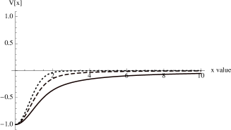
Figure 1: The potential $V$, as a function of $x={\textstyle{r\over{2\sqrt{\theta}}}}$. $d_{U}=1.1,1.5$ and $1.9$, are represented by the solid, dashed and dotted lines.

4 Final Remarks

To conclude, let us our work in its proper perspective. As was showed, our analysis revealed that even if the Higgs field takes a non-vanishing v.e.v., gauge interaction keeps its long range character leading to an effective gauge symmetry restoration. Besides, we have considered the effect of a minimal length on a physical observable in the un-particle sector. Interestingly enough, expression (LABEL:NCunp80) displays a marked departure from its commutative counterpart. Nevertheless, the above profile potential is similar to that encountered in ordinary space-time as $L\to\infty$. Therefore, we have provided a new connection between effective models.

Finally, we would like to comment our results from the vantage point of the space-time ”fractalization” outlined in [32], where the concept of un-spectral dimension was introduced for the first time. The authors in [32] proposed a new scenario merging the conjectured existence of both un-particles and minimal length in the space-time fabric. In this case, the minimal length plays a role which is similar to the critical temperature marking different phases of some condensed matter system. The use of un-particle probes allows the access to a trans-planckian regime which is forbidden to ordinary matter. In this ultimate phase the un-spectral space-time dimension is $D_{u}=2d_{u}-2$. We notice that the distance dependence of the interaction potential (31) is just $1/L^{D_{u}}$, i.e. test charges are sensitive to the un-spectral dimension. We consider this behavior as a self-consistency check with the model discussed in [32].

References

• [1] H. Georgi, Phys. Rev. Lett.  98, (2007) 221601.
• [2] H. Georgi, Phys. Lett. B 650, (2007) 275.
• [3] Y. Nakayama, Phys. Rev. D 76, (2007) 105009.
• [4] H. Zhang, C. S. Li and Z. Li, Phys. Rev. D 76, (2007) 116003.
• [5] Y. Liao and J. -Y. Liu, Phys. Rev. Lett.  99, (2007) 191804.
• [6] T. Kikuchi and N. Okada, Phys. Lett. B 665, (2008) 186.
• [7] N. G. Deshpande, X. -G. He and J. Jiang, Phys. Lett. B 656, (2007) 91.
• [8] J. R. Mureika, Phys. Lett. B 660, (2008) 561.
• [9] J. R. Mureika, Phys. Rev. D 79 (2009) 056003.
• [10] J. R. Mureika, Int. J. Theor. Phys.  51 (2012) 1259.
• [11] J. R. Mureika and E. Spallucci, Phys. Lett. B 693, (2010) 129.
• [12] P. Gaete, J. A. Helayel-Neto and E. Spallucci, Phys. Lett. B 693, (2010) 155.
• [13] C. M. Ho and Y. Nakayama, JHEP 0905, (2009) 081.
• [14] R. Mohanta and A. K. Giri, Phys. Rev. D 76, (2007) 057701.
• [15] A. T. Alan and N. K. Pak, Europhys. Lett.  84, (2008) 11001.
• [16] T. M. Aliev, M. Frank and I. Turan, Phys. Rev. D 80, (2009) 114019.
• [17] M. C. Kumar, P. Mathews, V. Ravindran and A. Tripathi, Phys. Rev. D 77, (2008) 055013.
• [18] A. M. Frassino, P. Nicolini and O. Panella, “Un-Casimir effect”, arXiv:1311.7173 [hep-ph].
• [19] P. J. Fox, A. Rajaraman and Y. Shirman, Phys. Rev. D 76, (2007) 075004.
• [20] A. Delgado, J. R. Espinosa and M. Quiros, JHEP 0710, (2007) 094.
• [21] T. Kikuchi and N. Okada, Phys. Lett. B 661, (2008) 360.
• [22] F. Sannino, Acta Phys. Polon. B 40, (2009) 3533.
• [23] G. Amelino-Camelia, Nature 418, (2002) 34.
• [24] T. Jacobson, S. Liberati and D. Mattingly, Phys. Rev. D 67, (2003) 124011.
• [25] T. J. Konopka and S. A. Major, New J. Phys.  4, (2002) 57.
• [26] S. Hossenfelder, Phys. Rev. D 73, (2006) 105013.
• [27] P. Nicolini, Int. J. Mod. Phys. A 24, (2009) 1229.
• [28] P. Nicolini, A. Smailagic and E. Spallucci, Phys. Lett. B 632, (2006) 547.
• [29] M. B. Green, J. H. Schwarz and E. Witten: Superstring Theory. Cambridge University Press, Cambridge (1987).
• [30] J. Magueijo and L. Smolin, Phys. Rev. Lett.  88, (2002) 190403.
• [31] S. Hossenfelder, M. Bleicher, S. Hofmann, J. Ruppert, S. Scherer and H. Stoecker, Phys. Lett. B 575, (2003) 85.
• [32] P. Nicolini and E. Spallucci, Phys. Lett. B 695, (2011) 290.
• [33] M. Sprenger, P. Nicolini and M. Bleicher, Eur. J. Phys.  33, (2012) 853.
• [34] E. Witten, Nucl. Phys.  B 268, (1986) 253.
• [35] N. Seiberg and E. Witten, JHEP 9909, (1999) 032.
• [36] M. R. Douglas, N. A. Nekrasov, Rev. Mod. Phys.  73, (2001) 977-1029.
• [37] R. J. Szabo, Phys. Rept.  378, (2003) 207-299.
• [38] J. Gomis, K. Kamimura and T. Mateos, JHEP 0103, (2001) 010.
• [39] A. A. Bichl, J. M. Grimstrup, L. Popp, M. Schweda and R. Wulkenhaar, Int. J. Mod. Phys.  A 17, (2002) 2219.
• [40] A. Smailagic and E. Spallucci, J. Phys. A 36, (2003) L517.
• [41] A. Smailagic and E. Spallucci, J. Phys. A 36, (2003) L467.
• [42] A. Smailagic and E. Spallucci, J. Phys. A 37, (2004) 1 [Erratum-ibid.  A 37, (2004) 7169].
• [43] A. B. Hammou, M. Lagraa and M. M. Sheikh-Jabbari, Phys. Rev. D 66, (2002) 025025.
• [44] P. Gaete and E. Spallucci, “Gauge symmetry restoration in the un-particle vacuum”, arXiv:1205.2248 [hep-th].
• [45] P. Gaete and E. Spallucci, Phys. Lett. B 661, (2008) 319.
• [46] N. V. Krasnikov, Int. J. Mod. Phys. A 22, (2007) 5117.
• [47] P. Gaete and E. Spallucci, Phys. Lett. B 668, (2008) 336.
• [48] P. Gaete and E. Spallucci, J. Phys. A 45, (2012) 065401.
• [49] P. Gaete, J.  Helayel-Neto and E. Spallucci, J. Phys. A 45, (2012) 215401.
• [50] E. Spallucci, A. Smailagic and P. Nicolini, Phys. Rev. D 73, (2006) 084004.
• [51] L. Modesto, J. W. Moffat and P. Nicolini, Phys. Lett. B 695, (2011) 397.
• [52] P. Nicolini, “Nonlocal and generalized uncertainty principle black holes”, arXiv:1202.2102 [hep-th].