Estimation in a change-point nonlinear quantile model

ABSTRACT. This paper considers a nonlinear quantile model with change-points. The quantile estimation method, which as a particular case includes median model, is more robust with respect to other traditional methods when model errors contain outliers. Under relatively weak assumptions, the convergence rate and asymptotic distribution of change-point and of regression parameter estimators are obtained. Numerical study by Monte Carlo simulations shows the performance of the proposed method for nonlinear model with change-points.

Keywords: Multiple change-points; Quantile regression; Asymptotic behaviour.
Mathematics Subject Classification: Primary 62F10, 62F12 ; Secondary 62J02.

1 Introduction

Classically, for linear or nonlinear models, the errors are supposed with mean zero and bounded variance. In this case, model parameters are estimated generally by least squares (LS) method. If these conditions are not satisfied or if model contains outliers, then the LS estimators of the model parameters can have a large error. A very interesting and robust alternative method was proposed by Koenker and Bassett (1978) by the introduction of the quantile method. A particular case of this method is that of least absolute deviation (LAD). For a complete overview on quantile method, we refer the reader to book of Koenker (2005). Properties of a nonlinear quantile model are studied also in the papers Chen et al. (2013), Choi et al. (2005), Oberhofer and Haupt (2014).
     On the other hand, in applications, it is possible that we have not one but several models, the localization where model changes being unknown. We obtain which is called as a change-point model. The purpose of this paper is to study the properties of this type of model estimated by quantile method, when between two consecutive change-points the model is nonlinear. For this study we need to known the asymptotic behaviour of the objective function.
     To our knowledge, most previous studies of change-point models have focused on linear models. On this subject, we can mention the following papers: Bai (1998) for LAD method, Bai and Perron (1998) for LS method, Koul and Qian (2002) for maximum likelihood method, Koul et al. (2003) for M-estimation method. For quantile method, Oka and Qu (2011) estimate the change-points location and the coefficient parameters of each phase, Furno (2012) realize a Lagrange multiplier test for detecting the structural breaks. For change-point nonlinear model, because of difficulties caused by the nonlinearity, literature is less rich: Boldea and Hall (2013) use LS method to estimate and test the number of breaks. In Ciuperca (2009), the M-estimation method is used to estimate a multiphase nonlinear model with random design and changes in the model due to some (unknown) values in design. A general criterion is proposed in Ciuperca (2011a) to determine the change-point number. If changes in the model occur in time, the LAD estimation method was studied by Ciuperca (2011b).
     Present paper generalizes Ciuperca (2011b), considering a method, for estimating and for choosing the change-point number criterion, based on the quantile framework. This is because, often in practice, especially in the case of change-point models, the quantile index $\tau$ of errors is not 1/2.
     We note the important fact that, in a multiple change-point model, the change-point estimation could affects the estimator properties. Moreover, it is difficult to study, theoretically but also numerically, a change-point model since it depends of two parameter types: the regression parameters and the change-points.
     The plan of this paper is as follows. In Section 2 we first introduce some notations and assumptions. Next, we study the asymptotic behaviour of the objective function. In Section 3, we define and study the quantile estimator in a nonlinear model with change-points. Convergence rate and asymptotic distributions of the estimators are obtained. Finally, in Section 4, simulation results illustrate the performance of the quantile method for change-point nonlinear model. In Appendix Bernstein’s inequality is recalled.

2 Quantile regression without change

In this section we study the asymptotic behaviour of the quantile process.

Let us consider the following regression model

$$Y_{i}=g(\textrm{$\mathbf{X}$}_{i},\textrm{$\mathbf{\phi}$})+\varepsilon_{i},\qquad i=1,\cdots,n,$$ (1)

where the regression function $g:\Upsilon\times\Gamma\rightarrow\mathbb{R}$, with $\textrm{$\mathbf{\phi}$}\in\Gamma\subseteq\mathbb{R}^{p}$, $\textrm{$\mathbf{x}$}\in\Upsilon$, $\Upsilon\subseteq\mathbb{R}^{d}$ is known up to the parameter $\mathbf{\phi}$. We suppose that the set $\Gamma$ is compact.
     For a fixed quantile index $\tau\in(0,1)$, the $\tau$th conditional quantile regression of $Y$, given $\mathbf{x}$, is $g(\textrm{$\mathbf{x}$},\textrm{$\mathbf{\phi}$})+F^{-1}(\tau)$, with $F^{-1}(\tau)$ the $\tau$th quantile ($F^{-1}$ is the inverse of the distribution function $F$) of error $\varepsilon$. We suppose that $F(0)=\tau$.
In the case when the model contains intercept, noted $\phi_{0}$, the regression function has the form $g(\textrm{$\mathbf{x}$},\textrm{$\mathbf{\phi}$})=\phi_{0}+g_{0}(\textrm{$\mathbf{x}$},\textrm{$\mathbf{\phi}$}_{1})$. Then, the following parameter vector is considered $\textrm{$\mathbf{\phi}$}(\tau)=(\phi_{0}(\tau),\textrm{$\mathbf{\phi}$}_{1})^{t}$, with $\phi_{0}(\tau)=\phi_{0}+F^{-1}(\tau)$. Thus, when model contains an intercept $\phi_{0}$, we estimate first $\phi_{0}(\tau)$ from which we then have the estimation of $\phi_{0}$. For linear models, in literature, the presence or not of intercept intervenes in the result proofs (see for example Oka and Qu (2011)).
     The estimator of $\textrm{$\mathbf{\phi}$}(\tau)$ by Koenker and Bassett technique (see Koenker and Bassett (1978)) is called quantile regression. We suppose $\tau$ fixed, therefore, for simplicity reasons, we will note $\textrm{$\mathbf{\phi}$}(\tau)$ by $\mathbf{\phi}$. Contrary to the papers where linear models are studied (see for example Oka and Qu (2011)) when $\phi_{0}\neq 0$, in this paper we shall consider simultaneously the two cases presented above.

2.1 Assumptions and notations

In this subsection we give assumptions and notations needed in this paper.
     For simplicity, we suppose that the regressors $\textrm{$\mathbf{X}$}_{i}$ are non random, although the results will, typically hold for random $\textrm{$\mathbf{X}$}_{i}$’s independent of the $\varepsilon_{i}$’s and if $\textrm{$\mathbf{X}$}_{i}$ independent of $\textrm{$\mathbf{X}$}_{j}$ for $i\neq j$.
For the model (1), we consider $\textrm{$\mathbf{\phi}$}^{0}$ the true value (unknown) of $\mathbf{\phi}$, with $\mathbf{\phi^{0}}$ an inner point of the compact $\Gamma$.
For a fixed quantile index $\tau\in(0,1)$, consider the check function $\rho:\mathbb{R}\rightarrow\mathbb{R}$ given by

$$\rho_{\tau}(u)=u[\tau-1\!\!1_{u\leq 0}]$$

and random variable

$$D_{i}(\tau)\equiv\tau-1\!\!1_{\varepsilon_{i}\leq 0}.$$

Since $F(0)=\tau$ we have $I\!\!E[D_{i}(\tau)]=0$.
     The quantile estimator of parameter $\mathbf{\phi}$ is defined by

$$\hat{\textrm{$\mathbf{\phi}$}}_{n}^{(\tau)}\equiv\mathop{\mathrm{arg\,min}}_{\textrm{$\mathbf{\phi}$}\in\Gamma}\sum^{n}_{i=1}\rho_{\tau}(Y_{i}-g(\textrm{$\mathbf{X}$}_{i},\textrm{$\mathbf{\phi}$})).$$ (2)

Its consistency, with $n^{-1/2}$ convergence rate and asymptotic normality of estimator $\hat{\textrm{$\mathbf{\phi}$}}_{n}^{(\tau)}$ have been proved in previous papers (see for example Koenker (2005)).

For reading convenience, all throughout the paper, let us consider the following notation, for all $\textrm{$\mathbf{\phi}$}\in\Gamma$ and $i=1,\cdots,n$,

$$h_{i}(\textrm{$\mathbf{\phi}$})\equiv g(\textrm{$\mathbf{X}$}_{i},\textrm{$\mathbf{\phi}$})-g(\textrm{$\mathbf{X}$}_{i},\textrm{$\mathbf{\phi}$}^{0}).$$

In order to study the quantile model, let us consider the following two random processes:

$$\left\{\begin{array}[]{l}\displaystyle{W_{n}(\tau;\textrm{$\mathbf{\phi}$},\textrm{$\mathbf{\phi^{0}}$})\equiv-\sum^{n}_{i=1}D_{i}(\tau)h_{i}(\textrm{$\mathbf{\phi}$})},\\ \displaystyle{Z_{n}(\textrm{$\mathbf{\phi}$},\textrm{$\mathbf{\phi^{0}}$})\equiv\sum^{n}_{i=1}\int^{h_{i}(\textrm{$\mathbf{\phi}$})}_{0}(1\!\!1_{\varepsilon_{i}\leq s}-1\!\!1_{\varepsilon_{i}\leq 0})ds.}\end{array}\right.$$ (3)

Obviously $I\!\!E[W_{n}(\tau;\textrm{$\mathbf{\phi}$},\textrm{$\mathbf{\phi^{0}}$})]=0$.
     For each sample $i\in\{1,\cdots,n\}$, in order to study always the quantile model, consider the following difference

$$G_{i}^{(\tau)}(\textrm{$\mathbf{\phi}$},\textrm{$\mathbf{\phi}$}^{0})\equiv\rho_{\tau}(\varepsilon_{i}-g(\textrm{$\mathbf{X}$}_{i},\textrm{$\mathbf{\phi}$})+g(\textrm{$\mathbf{X}$}_{i},\textrm{$\mathbf{\phi}$}^{0}))-\rho_{\tau}(\varepsilon_{i}),$$

from which us define the random process

$${\cal G}^{(\tau)}_{n}(\textrm{$\mathbf{\phi}$},\textrm{$\mathbf{\phi}$}^{0})\equiv\sum^{n}_{i=1}G_{i}^{(\tau)}(\textrm{$\mathbf{\phi}$},\textrm{$\mathbf{\phi}$}^{0}),$$

which is in fact the objective function for finding the quantile estimator $\hat{\textrm{$\mathbf{\phi}$}}^{(\tau)}_{n}$ of model (1).
Using identity of Knight (1998), for any real nonzero number $r$, we have that $\rho_{\tau}(r-s)-\rho_{\tau}(r)=s[1\!\!1_{r<0}-\tau]+\int^{s}_{0}[1\!\!1_{r\leq t}-1\!\!1_{r\leq 0}]dt$. Then, the process ${\cal G}^{(\tau)}_{n}(\textrm{$\mathbf{\phi}$},\textrm{$\mathbf{\phi}$}^{0})$ can also write as

$${\cal G}^{(\tau)}_{n}(\textrm{$\mathbf{\phi}$},\textrm{$\mathbf{\phi}$}^{0})=W_{n}(\tau;\textrm{$\mathbf{\phi}$},\textrm{$\mathbf{\phi^{0}}$})+Z_{n}(\textrm{$\mathbf{\phi}$},\textrm{$\mathbf{\phi^{0}}$}).$$ (4)

In the case of a nonlinear model, function ${\cal G}^{(\tau)}_{n}(\textrm{$\mathbf{\phi}$},\textrm{$\mathbf{\phi}$}^{0})$ is not convex in $\mathbf{\phi}$ which means that the study of estimator $\hat{\textrm{$\mathbf{\phi}$}}_{n}^{(\tau)}$ and of function ${\cal G}^{(\tau)}_{n}(\textrm{$\mathbf{\phi}$},\textrm{$\mathbf{\phi}$}^{0})$ will be different than for a linear model, based on the convexity.

All throughout the paper, C denotes a positive generic constant which may take different values in different formula or even in different parts of the same formula. All vectors are column and $\textbf{v}^{t}$ denotes the transposed of v. All vectors and matrices are in bold. Concerning the used norms, for a m-vector $\mathbf{{v}}=(v_{1},\cdots,v_{m})$, let us denote by $\|\mathbf{{v}}\|_{1}=\sum_{j=1}^{m}|v_{j}|$ and $\|\mathbf{{v}}\|_{2}=(\sum_{j=1}^{m}v^{2}_{j})^{1/2}$. For a matrix $\textbf{M}=(a_{ij})_{\begin{subarray}{c}1\leqslant i\leqslant m_{1}\\ 1\leqslant j\leqslant m_{2}\end{subarray}}$, we denote by $\|\textbf{M}\|_{1}=\max_{j=1,\cdots,m_{2}}(\sum_{i=1}^{m_{1}}|a_{ij}|)$, the subordinate norm to the vector norm $\|.\|_{1}$.

We now state the assumptions on the errors and on the regression function.
     The errors $(\varepsilon_{i})_{1\leq i\leq n}$ are supposed independent identically distributed (i.i.d.) random variables. We denote by $f$ the density and by $F$ the distribution function of $\varepsilon$.
(A1) There exists two constants $c_{0}>0$ and $\delta_{0}>0$ such that for all $|x|\leq\delta_{0}$, we have

$$\min(F(|x|)-F(0),F(0)-F(-|x|))\geq c_{0}|x|.$$

Contrary to the classic assumptions for a nonlinear regression model, we do not impose the condition that the mean of errors $\varepsilon_{i}$ is zero or that their variance is bounded.
     The regression function $g(\textrm{$\mathbf{x}$},\textrm{$\mathbf{\phi}$})$ is supposed twice differentiable in $\mathbf{\phi}$ and continuous on $\Upsilon$. In the following, for $\textrm{$\mathbf{x}$}\in\Upsilon$ and $\textrm{$\mathbf{\phi}$}\in\Gamma$ we use notation $\overset{.}{\textbf{g}}(\textrm{$\mathbf{x}$},\textrm{$\mathbf{\phi}$})\equiv\partial g(\textrm{$\mathbf{x}$},\textrm{$\mathbf{\phi}$})/\partial\textrm{$\mathbf{\phi}$}$ and $\overset{..}{\textbf{g}}(\textrm{$\mathbf{x}$},\textrm{$\mathbf{\phi}$})\equiv\partial^{2}g(\textrm{$\mathbf{x}$},\textrm{$\mathbf{\phi}$})/\partial\textrm{$\mathbf{\phi}$}^{2}$. Moreover, for the function $g$, following assumptions are considered:
(A2) For all $\textrm{$\mathbf{x}$}\in\Upsilon$, function $\overset{.}{\textbf{g}}(\textrm{$\mathbf{x}$},\textrm{$\mathbf{\phi}$})$ is bounded in every $\eta$-neighbourhood of $\mathbf{\phi^{0}}$, when $\eta\rightarrow 0$.
(A3) There exists $c_{1}>0$ such that $n^{-1}\sum^{n}_{i=1}\sup_{\textrm{$\mathbf{\phi}$}\in\Gamma}\|\overset{.}{\textbf{g}}(\textrm{$\mathbf{X}$}_{i},\textrm{$\mathbf{\phi}$})\|_{2}\leq c_{1}<\infty$.
(A4) There exist two positive constants $c_{2},c_{3}>0$ and natural $n_{0}$ such that for all $\textrm{$\mathbf{\phi}$}_{1},\textrm{$\mathbf{\phi}$}_{2}\in\Gamma$ and $n\geq n_{0}$: $c_{2}\|\textrm{$\mathbf{\phi}$}_{1}-\textrm{$\mathbf{\phi}$}_{2}\|_{2}\leq\left(n^{-1}\sum^{n}_{i=1}[g(\textrm{$\mathbf{X}$}_{i},\textrm{$\mathbf{\phi}$}_{1})-g(\textrm{$\mathbf{X}$}_{i},\textrm{$\mathbf{\phi}$}_{2})]^{2}\right)^{1/2}\leq c_{3}\|\textrm{$\mathbf{\phi}$}_{1}-\textrm{$\mathbf{\phi}$}_{2}\|_{2}.$ Moreover, we have $n^{-1}\sum^{n}_{i=1}\overset{.}{\textbf{g}}(\textrm{$\mathbf{X}$}_{i},\textrm{$\mathbf{\phi^{0}}$})\overset{.}{\textbf{g}}^{t}(\textrm{$\mathbf{X}$}_{i},\textrm{$\mathbf{\phi^{0}}$})$ converges, as $n\rightarrow\infty$, to a positive definite matrix. Furthermore, $\max_{1\leq i\leq n}n^{-1/2}\|\overset{.}{\textbf{g}}(\textrm{$\mathbf{X}$}_{i},\textrm{$\mathbf{\phi^{0}}$})\|_{2}\rightarrow 0$.
(A5) For all $\textrm{$\mathbf{x}$}\in\Upsilon$, $\textrm{$\mathbf{\phi}$}\in{\cal V}_{\eta}(\textrm{$\mathbf{\phi^{0}}$})$, with $\eta\rightarrow 0$, we have that $\|\overset{..}{\textbf{g}}(\textrm{$\mathbf{x}$},\textrm{$\mathbf{\phi}$})\|_{1}$ is bounded.
For certain results, stronger assumptions are necessary:
(A6) For all $\textrm{$\mathbf{\phi}$}\in\Gamma$, $\textrm{$\mathbf{x}$}\in\Upsilon$, we have that $\|\overset{.}{\textbf{g}}(\textrm{$\mathbf{x}$},\textrm{$\mathbf{\phi}$})\|_{2}$ is bounded.
(A7) For all $\textrm{$\mathbf{\phi}$}\in\Gamma$, $\textrm{$\mathbf{x}$}\in\Upsilon$, we have that $\|\overset{..}{\textbf{g}}(\textrm{$\mathbf{x}$},\textrm{$\mathbf{\phi}$})\|_{1}$ is bounded.

We wish to emphasise the fact that, with respect to the particular case $\tau=1/2$, considered in Ciuperca (2011b), we consider here multidimensional regressors $\textrm{$\mathbf{X}$}_{i}$.
     Assumption (A2) means that for every $\eta\rightarrow 0$, the function $\|\overset{.}{\textbf{g}}(\textrm{$\mathbf{x}$},\textrm{$\mathbf{\phi}$})\|_{2}$ is bounded for all $\textrm{$\mathbf{x}$}\in\Upsilon$ and for all $\textrm{$\mathbf{\phi}$}\in{\cal V}_{\eta}$, with

$${\cal V}_{\eta}\equiv\{\textrm{$\mathbf{\phi}$}\in\Gamma;\|\textrm{$\mathbf{\phi}$}-\textrm{$\mathbf{\phi^{0}}$}\|_{2}\leq\eta\}.$$

Assumptions (A1), (A4) are needed that the objective function has an unique minimum at $\mathbf{\phi^{0}}$ and for convergence and asymptotic normality of the quantile estimator (see Koenker (2005), page 124). Obviously that, assumption (A7) implies (A5). We have also that (A6) implies (A2), (A3) and third condition of (A4).
Note that assumption (A3) is the same as in paper Ciuperca (2011b), for a median nonlinear model and (A1) is supposition (C4) of Oberhofer and Haupt (2014)’s paper, for a nonlinear quantile regression with weakly dependent errors. As noted in the last paper, assumption (A1) is stronger that the usual assumption in literature: $f(x)$ exists in a neighbourhood of $x=0$ and $f(0)\geq c_{0}>0$.

2.2 Asymptotic behaviour of objective function ${\cal G}_{n}^{(\tau)}(\textrm{$\mathbf{\phi}$},\textrm{$\mathbf{\phi^{0}}$})$

In order to study the main part of this paper devoted to a change-point model estimated by quantile framework, in this subsection the asymptotic behaviour of process ${\cal G}_{n}^{(\tau)}(\textrm{$\mathbf{\phi}$},\textrm{$\mathbf{\phi^{0}}$})$ is studied.
     Recall that under assumptions (A1) and (A4), the quantile estimator $\hat{\textrm{$\mathbf{\phi}$}}^{(\tau)}_{n}$, given by (2), is weakly $n^{-1/2}$-consistent (see Koenker (2005) or Oberhofer (1982)).

Remark 2.1

By elementary calculations we show that, for all $\textrm{$\mathbf{\phi}$}\in\Gamma$:

• if $h_{i}(\textrm{$\mathbf{\phi}$})\geq 0$ we have

  $$\int_{0}^{h_{i}(\textrm{$\mathbf{\phi}$})}1\!\!1_{\varepsilon_{i}<t}dt=h_{i}(\textrm{$\mathbf{\phi}$})1\!\!1_{\varepsilon_{i}<0}+[h_{i}(\textrm{$\mathbf{\phi}$})-\varepsilon_{i}]1\!\!1_{0\leq\varepsilon_{i}\leq h_{i}(\textrm{$\mathbf{\phi}$})}+0\cdot 1\!\!1_{\varepsilon_{i}>h_{i}(\textrm{$\mathbf{\phi}$})},$$

• if $h_{i}(\textrm{$\mathbf{\phi}$})<0$ we have

  $$\int_{0}^{h_{i}(\textrm{$\mathbf{\phi}$})}1\!\!1_{\varepsilon_{i}<t}dt=0\cdot 1\!\!1_{\varepsilon_{i}>0}-\varepsilon_{i}1\!\!1_{h_{i}(\textrm{$\mathbf{\phi}$})\leq\varepsilon_{i}\leq 0}+h_{i}(\textrm{$\mathbf{\phi}$})1\!\!1_{\varepsilon_{i}<0}.$$

These imply that

• if $h_{i}(\textrm{$\mathbf{\phi}$})\geq 0$ we have
  

  $$\int_{0}^{h_{i}(\textrm{$\mathbf{\phi}$})}[1\!\!1_{\varepsilon_{i}<t}-1\!\!1_{\varepsilon_{i}<0}]dt=[h_{i}(\textrm{$\mathbf{\phi}$})-\varepsilon_{i}]1\!\!1_{0\leq\varepsilon_{i}\leq h_{i}(\textrm{$\mathbf{\phi}$})},$$

• if $h_{i}(\textrm{$\mathbf{\phi}$})<0$ we have

  $$\int_{0}^{h_{i}(\textrm{$\mathbf{\phi}$})}[1\!\!1_{\varepsilon_{i}<t}-1\!\!1_{\varepsilon_{i}<0}]dt=[-\varepsilon_{i}-h_{i}(\textrm{$\mathbf{\phi}$})]1\!\!1_{h_{i}(\textrm{$\mathbf{\phi}$})\leq\varepsilon_{i}\leq 0}.$$

Thus, for $Z_{n}(\textrm{$\mathbf{\phi}$},\textrm{$\mathbf{\phi^{0}}$})$ defined by (3), we have with probability one that, $Z_{n}(\textrm{$\mathbf{\phi}$},\textrm{$\mathbf{\phi^{0}}$})\geq 0$ for all $\textrm{$\mathbf{\phi}$}\in\Gamma$.

A consequence of this remark, taking into account that $I\!\!E[W_{n}(\tau;\textrm{$\mathbf{\phi}$},\textrm{$\mathbf{\phi^{0}}$})]=0$ for all $\textrm{$\mathbf{\phi}$}\in\Gamma$, is that

$$I\!\!E[{\cal G}_{n}^{(\tau)}(\textrm{$\mathbf{\phi}$},\textrm{$\mathbf{\phi^{0}}$})]\geq 0,\qquad\textrm{ for all }\textrm{$\mathbf{\phi}$}\in\Gamma.$$ (5)

We will now study the asymptotic behaviour of the objective function ${\cal G}_{n}^{(\tau)}(\textrm{$\mathbf{\phi}$},\textrm{$\mathbf{\phi^{0}}$})$. In this purpose, for a bounded deterministic sequence $c_{n}$, let us consider the following parameter set:

$$\Omega_{c_{n}}\equiv\{\textrm{$\mathbf{\phi}$}\in\Gamma;\|\textrm{$\mathbf{\phi}$}-\textrm{$\mathbf{\phi^{0}}$}\|_{2}\leq c_{n}\}.$$

Emphasize that for the following Proposition, claim (i), the sequence $(c_{n})$ is a constant $c$. Thus, we denote the set $\Omega_{c_{n}}$ by $\Omega_{c}$. The proof idea is the same as in Bai (1998), Lemma 4, only now the nonlinearity of $g(\textrm{$\mathbf{x}$},\textrm{$\mathbf{\phi}$})$ and the quantile regression intervene significantly.

Proposition 2.1

Let us consider a deterministic positive sequence $(a_{n})$ such that $a_{n}\rightarrow\infty$, as $n\rightarrow\infty$.
(i) Under assumption (A6), if sequence $(a_{n})$ satisfies in addition the conditions $n^{-1}a_{n}=O(1)$, $n^{-1}a_{n}^{2}/\log n\rightarrow\infty$ as $n\rightarrow\infty$, and the parameters belong to the set $\Omega_{c}=\{\textrm{$\mathbf{\phi}$}\in\Gamma;\|\textrm{$\mathbf{\phi}$}-\textrm{$\mathbf{\phi^{0}}$}\|_{2}\leq c\}$, we have that, for all $\epsilon>0$, there exists a constant $C>0$ and a natural number $n_{\epsilon}\in\mathbb{N}$ such that for all $n\geq n_{\epsilon}$,

$$I\!\!P\left[\sup_{\textrm{$\mathbf{\phi}$}\in\Omega_{c}}\left|\frac{1}{a_{n}}\left[{\cal G}_{n}^{(\tau)}(\textrm{$\mathbf{\phi}$},\textrm{$\mathbf{\phi^{0}}$})-I\!\!E[{\cal G}_{n}^{(\tau)}(\textrm{$\mathbf{\phi}$},\textrm{$\mathbf{\phi^{0}}$})]\right]\right|>\epsilon\right]\leq\exp(-C\epsilon^{2}n^{-1}a^{2}_{n}).$$

(ii) Under assumptions (A2), (A3), if we have furthermore an another sequence $(c_{n})$ such that $c_{n}\rightarrow 0$, $n^{-1}c^{-1}_{n}a_{n}=O(1)$, $a_{n}^{2}/(nc_{n}^{2}\log n)\rightarrow\infty$ as $n\rightarrow\infty$ and the parameters belong to the set $\Omega_{c_{n}}$, we have that, for all $\epsilon>0$, there exists a constant $C>0$ and a natural number $n_{\epsilon}\in\mathbb{N}$ such that for all $n\geq n_{\epsilon}$,

$$I\!\!P\left[\sup_{\textrm{$\mathbf{\phi}$}\in\Omega_{c_{n}}}\left|\frac{1}{a_{n}}\left[{\cal G}_{n}^{(\tau)}(\textrm{$\mathbf{\phi}$},\textrm{$\mathbf{\phi^{0}}$})-I\!\!E[{\cal G}_{n}^{(\tau)}(\textrm{$\mathbf{\phi}$},\textrm{$\mathbf{\phi^{0}}$})]\right]\right|>\epsilon\right]\leq\exp(-C\epsilon^{2}n^{-1}c_{n}^{-2}a^{2}_{n}).$$

Proof. (i) We decompose $\Omega_{c}$ in subsets, such that the diameter of each subset is less than $cn^{-1/2}$. Thus, we can write $\Omega_{c}=\cup^{C_{p}n^{p/2}}_{j=1}\omega_{j}^{n}$, where $\omega^{n}_{j}\equiv\{\textrm{$\mathbf{\phi}$}\in\Omega_{c};\|\textrm{$\mathbf{\phi}$}-\textrm{$\mathbf{\phi}$}_{j}\|_{2}\leq cn^{-1/2}\}$, with $\textrm{$\mathbf{\phi}$}_{j}\in\Omega_{c}$. This decomposition depends on the dimension of the parameter set $\Gamma$, then positive constant $C_{p}$($<\infty$) depends on $p$. Diameter $cn^{-1/2}$ of each cell $\omega^{n}_{j}$ was taken as that, for two points belonging to the same cell, the difference which occurs in the left hand side of following relation (6) converges to 0 as $n\rightarrow\infty$. Then, in order to study the behaviour of ${\cal G}_{n}^{(\tau)}(\textrm{$\mathbf{\phi}$},\textrm{$\mathbf{\phi^{0}}$})-I\!\!E[{\cal G}_{n}^{(\tau)}(\textrm{$\mathbf{\phi}$},\textrm{$\mathbf{\phi^{0}}$})]$ for all $\textrm{$\mathbf{\phi}$}\in\Gamma$, we take one representative point, noted $\textrm{$\mathbf{\phi}$}_{j}$, of $\omega^{n}_{j}$, for each $j=1,\cdots,C_{p}n^{p/2}$. Then, in order to study the probability of the left hand side of claim (i) we just study the probability of the left hand side of (7).
Since $n^{-1}a_{n}^{2}/\log n\rightarrow\infty$, then we have that $n^{-1/2}a_{n}\rightarrow\infty$ as $n\rightarrow\infty$. Thus, for each $\textrm{$\mathbf{\phi}$}_{1},\textrm{$\mathbf{\phi}$}_{2}\in\omega^{n}_{j}$, using assumption $n^{-1}\sum^{n}_{i=1}\sup_{\textrm{$\mathbf{\phi}$}\in\Gamma}$ $\|\overset{.}{\textbf{g}}(\textrm{$\mathbf{X}$}_{i},\textrm{$\mathbf{\phi}$})\|_{2}\leq c_{1}<\infty$ of (A6), we have

$$\begin{array}[]{l}a_{n}^{-1}|{\cal G}_{n}^{(\tau)}(\textrm{$\mathbf{\phi}$}_{1},\textrm{$\mathbf{\phi^{0}}$})-I\!\!E[{\cal G}_{n}^{(\tau)}(\textrm{$\mathbf{\phi}$}_{1},\textrm{$\mathbf{\phi^{0}}$})]-{\cal G}_{n}^{(\tau)}(\textrm{$\mathbf{\phi}$}_{2},\textrm{$\mathbf{\phi^{0}}$})+I\!\!E[{\cal G}_{n}^{(\tau)}(\textrm{$\mathbf{\phi}$}_{2},\textrm{$\mathbf{\phi^{0}}$})]|\\ \qquad\qquad\qquad\leq Cna_{n}^{-1}\|\textrm{$\mathbf{\phi}$}_{1}-\textrm{$\mathbf{\phi}$}_{2}\|_{2}\leq Cn^{1/2}a_{n}^{-1}\rightarrow 0.\end{array}$$ (6)

For $\textrm{$\mathbf{\phi}$}_{j}\in\omega^{n}_{j}$, for any $j=1,\cdots,C_{p}n^{p/2}$, we have the following obvious inequality

$${I\!\!P\left[\sup_{j}a_{n}^{-1}|{\cal G}_{n}^{(\tau)}(\textrm{$\mathbf{\phi}$}_{j},\textrm{$\mathbf{\phi^{0}}$})-I\!\!E[{\cal G}_{n}^{(\tau)}(\textrm{$\mathbf{\phi}$}_{j},\textrm{$\mathbf{\phi^{0}}$})]|>\epsilon\right]}\displaystyle{\leq\sum^{C_{p}n^{p/2}}_{j=1}I\!\!P\left[|{\cal G}_{n}^{(\tau)}(\textrm{$\mathbf{\phi}$}_{j},\textrm{$\mathbf{\phi^{0}}$})-I\!\!E[{\cal G}_{n}^{(\tau)}(\textrm{$\mathbf{\phi}$}_{j},\textrm{$\mathbf{\phi^{0}}$})]|>\epsilon a_{n}\right].}$$ (7)

On the other hand, taking into account assumption (A6), we obtain that there exists a constant $C>0$ such that $|G_{i}^{(\tau)}(\textrm{$\mathbf{\phi}$}_{j},\textrm{$\mathbf{\phi^{0}}$})-I\!\!E[G_{i}^{(\tau)}(\textrm{$\mathbf{\phi}$}_{j},\textrm{$\mathbf{\phi^{0}}$})]|\leq C\|\textrm{$\mathbf{\phi}$}_{j}-\textrm{$\mathbf{\phi^{0}}$}\|_{2}\leq Cc$, with probability 1.
Moreover $\mathbb{V}\mbox{ar}\,[{\cal G}_{n}^{(\tau)}(\textrm{$\mathbf{\phi}$}_{j},\textrm{$\mathbf{\phi^{0}}$})]\leq Cnc^{2}$, with $C>0$.
Then, since $n^{-1}a_{n}=O(1)$, $a^{2}_{n}/(n\log n)\rightarrow\infty$ as $n\rightarrow\infty$, we can apply Bernstein’s inequality (24) (see Appendix), for $\beta=Cc$, $V=Cnc^{2}$, $s=1/2$, $z=a_{n}\epsilon$ and we obtain that

$$\begin{array}[]{ll}\displaystyle{\sum^{C_{p}n^{p/2}}_{j=1}I\!\!P[|{\cal G}_{n}^{(\tau)}(\textrm{$\mathbf{\phi}$}_{j},\textrm{$\mathbf{\phi^{0}}$})-I\!\!E[{\cal G}_{n}^{(\tau)}(\textrm{$\mathbf{\phi}$}_{j},\textrm{$\mathbf{\phi^{0}}$})]|>\epsilon a_{n}]}&\leq 2C_{p}n^{p/2}\exp(-C\epsilon^{2}n^{-1}a^{2}_{n})\\ &=2C_{p}\exp(-C\epsilon^{2}n^{-1}a^{2}_{n}+p/2\log n)\rightarrow 0,\end{array}$$

with $C>0$.
The claim follows combining the last relation together with (6) and (7).
     (ii) In this case, we decompose the set $\Omega_{c_{n}}=\cup^{C_{p}n^{p/2}}_{j=1}\omega_{j}^{n}$, with the subsets
$\omega^{n}_{j}\equiv\{\textrm{$\mathbf{\phi}$}\in\Omega_{c_{n}};\|\textrm{$\mathbf{\phi}$}-\textrm{$\mathbf{\phi}$}_{j}\|_{2}\leq c_{n}n^{-1/2}\}$, with $\textrm{$\mathbf{\phi}$}_{j}\in\Omega_{c_{n}}$.
Since $a^{2}_{n}/(nc^{2}_{n}\log n)\rightarrow\infty$ we have that $n^{1/2}c_{n}/a_{n}\rightarrow 0$ as $n\rightarrow\infty$. Then, for $\textrm{$\mathbf{\phi}$}_{1},\textrm{$\mathbf{\phi}$}_{2}\in\omega^{n}_{j}$ we have by similar arguments as in (6): $a_{n}^{-1}|{\cal G}_{n}^{(\tau)}(\textrm{$\mathbf{\phi}$}_{1},\textrm{$\mathbf{\phi^{0}}$})-I\!\!E[{\cal G}_{n}^{(\tau)}(\textrm{$\mathbf{\phi}$}_{1},\textrm{$\mathbf{\phi^{0}}$})]-{\cal G}_{n}^{(\tau)}(\textrm{$\mathbf{\phi}$}_{2},\textrm{$\mathbf{\phi^{0}}$})+I\!\!E[{\cal G}_{n}^{(\tau)}(\textrm{$\mathbf{\phi}$}_{2},\textrm{$\mathbf{\phi^{0}}$})]|\leq Cn^{1/2}c_{n}a_{n}^{-1}\rightarrow 0$, as $n\rightarrow\infty$.
On the other hand, for $\textrm{$\mathbf{\phi}$}_{j}\in\omega^{n}_{j}$, for any $j=1,\cdots,C_{p}n^{p/2}$, using assumption (A2), (A3) we have: $|G_{i}^{(\tau)}(\textrm{$\mathbf{\phi}$}_{j},\textrm{$\mathbf{\phi^{0}}$})-I\!\!E[G_{i}^{(\tau)}(\textrm{$\mathbf{\phi}$}_{j},\textrm{$\mathbf{\phi^{0}}$})]|\leq Cc_{n}$, with probability 1. The end of proof is similar to that of (i), using $\mathbb{V}\mbox{ar}\,[{\cal G}_{n}^{(\tau)}(\textrm{$\mathbf{\phi}$}_{j},\textrm{$\mathbf{\phi^{0}}$})]\leq Cnc^{2}_{n}$ and applying Bernstein’s inequality (24) for $\beta=Cc_{n}$, $V=Cnc^{2}_{n}$, $s=1/2$, $z=a_{n}\epsilon$. $\blacksquare$

Remark 2.2

An example of sequence $(a_{n})$ which satisfies the conditions of Proposition 2.1(i) is $a_{n}=n/(\log n)^{s}$, with $s\geq 0$.

Applying Proposition 2.1 and Borel-Cantelli lemma we obtain that for all $\epsilon>0$, we have

$$\limsup_{n\rightarrow\infty}\left(\sup_{\textrm{$\mathbf{\phi}$}\in\Omega_{c_{n}}}\frac{1}{a_{n}}\left|{\cal G}_{n}^{(\tau)}(\textrm{$\mathbf{\phi}$},\textrm{$\mathbf{\phi}$}^{0})-I\!\!E[{\cal G}_{n}^{(\tau)}(\textrm{$\mathbf{\phi}$},\textrm{$\mathbf{\phi}$}^{0})]\right|\right)\leq\epsilon,\qquad a.s.$$ (8)

which is the equivalent of Lemma A.2 of Oka and Qu (2011).

The following Proposition proves a general result that the infimum of objective function ${\cal G}_{n}^{(\tau)}(\textrm{$\mathbf{\phi}$},\textrm{$\mathbf{\phi}$}^{0})$ is strictely positive for $\mathbf{\phi}$ outside a ball centred at $\mathbf{\phi^{0}}$ with radius $w_{n}$ , when $w_{n}\rightarrow 0$.

Proposition 2.2

Suppose that assumptions (A1), (A4)-(A6) are satisfied, that density $f$ of $\varepsilon$ is differentiable in a neighbourhood of 0 and that $f^{\prime}(x)$ is bounded in this neighbourhood.
Let $(w_{n})$ be a monotone deterministic sequence converging to 0, such that $nw^{2}_{n}/\log n\rightarrow\infty$, as $n\rightarrow\infty$.
Then, there exists $\epsilon_{1}>0$ such that,

$$\liminf_{n\rightarrow\infty}\left(\inf_{\|\textrm{$\mathbf{\phi}$}-\textrm{$\mathbf{\phi}$}^{0}\|_{2}\geq w_{n}}\frac{1}{nw^{2}_{n}}{\cal G}_{n}^{(\tau)}(\textrm{$\mathbf{\phi}$},\textrm{$\mathbf{\phi}$}^{0})\right)>\epsilon_{1},$$

with probability 1.

Proof. Let us first consider a monotone positive sequence $(v_{n})$ such that $v_{n}\rightarrow 0$, as $n\rightarrow\infty$ and $v_{n}\geq w_{n}$ for $n$ large enough.
We now consider parameter $\mathbf{\phi}$ such that $\|\textrm{$\mathbf{\phi}$}-\textrm{$\mathbf{\phi^{0}}$}\|_{2}=v_{n}$. For a $p$-vector $\mathbf{u}$ in an open set of $\mathbb{R}^{p}$, with $\|\textrm{$\mathbf{u}$}\|_{2}=1$, we have using (4),

$$I\!\!E[{\cal G}^{(\tau)}_{n}(\textrm{$\mathbf{\phi^{0}}$}+v_{n}\textrm{$\mathbf{u}$},\textrm{$\mathbf{\phi^{0}}$})]=I\!\!E[Z_{n}(\textrm{$\mathbf{\phi^{0}}$}+v_{n}\textrm{$\mathbf{u}$},\textrm{$\mathbf{\phi^{0}}$})]=\sum^{n}_{i=1}\int^{h_{i}(\textrm{$\mathbf{\phi^{0}}$}+v_{n}\textrm{$\mathbf{u}$})}_{0}[F(s)-F(0)]ds.$$

We make the Taylor’s expansion for the distribution function $F$ and we obtain

$$I\!\!E[{\cal G}^{(\tau)}_{n}(\textrm{$\mathbf{\phi^{0}}$}+v_{n}\textrm{$\mathbf{u}$},\textrm{$\mathbf{\phi^{0}}$})]=\sum^{n}_{i=1}\int^{h_{i}(\textrm{$\mathbf{\phi^{0}}$}+v_{n}\textrm{$\mathbf{u}$})}_{0}sf(0)ds+\sum^{n}_{i=1}\int^{h_{i}(\textrm{$\mathbf{\phi^{0}}$}+v_{n}\textrm{$\mathbf{u}$})}_{0}\frac{s^{2}}{2}f^{\prime}(\zeta_{i}s)ds\equiv R_{1}+R_{2},$$ (9)

with $0<\zeta_{i}<1$.
The Taylor’s expansion up to order 1 of $g$ at $\textrm{$\mathbf{\phi}$}=\textrm{$\mathbf{\phi^{0}}$}$, the assumptions (A5), (A6) imply that $R_{1}$ is equal to

$$v^{2}_{n}\frac{f(0)}{2}\sum^{n}_{i=1}[\textrm{$\mathbf{u}$}^{t}\overset{.}{\textbf{g}}(\textrm{$\mathbf{X}$}_{i},\textrm{$\mathbf{\phi^{0}}$})+v_{n}\textrm{$\mathbf{u}$}^{t}\overset{..}{\textbf{g}}(\textrm{$\mathbf{X}$}_{i},\tilde{\textrm{$\mathbf{\phi}$}}_{i})\textrm{$\mathbf{u}$}]^{2}=v^{2}_{n}\frac{f(0)}{2}\sum^{n}_{i=1}[\textrm{$\mathbf{u}$}^{t}\overset{.}{\textbf{g}}(\textrm{$\mathbf{X}$}_{i},\textrm{$\mathbf{\phi^{0}}$})]^{2}(1+o(1)),$$ (10)

with $\tilde{\textrm{$\mathbf{\phi}$}}_{i}=\textrm{$\mathbf{\phi^{0}}$}+b_{i}v_{n}\textrm{$\mathbf{u}$}$, $b_{i}\in[0,1]$, $i=1,\cdots,n$.
For $R_{2}$, by similar arguments and since $f^{\prime}$ is bounded in the neighbourhood of 0, we have

$$|R_{2}|\leq C\sum^{n}_{i=1}\int^{|h_{i}(\textrm{$\mathbf{\phi^{0}}$}+v_{n}\textrm{$\mathbf{u}$})|}_{0}\frac{s^{2}}{2}ds=Cv^{3}_{n}\sum^{n}_{i=1}[\textrm{$\mathbf{u}$}^{t}\overset{.}{\textbf{g}}(\textrm{$\mathbf{X}$}_{i},\textrm{$\mathbf{\phi^{0}}$})]^{3}(1+o(1))=o(R_{1}).$$ (11)

Then, taking into account (9), (10) and (11) we obtain:

$$I\!\!E[{\cal G}^{(\tau)}_{n}(\textrm{$\mathbf{\phi^{0}}$}+v_{n}\textrm{$\mathbf{u}$},\textrm{$\mathbf{\phi^{0}}$})]=w^{2}_{n}\frac{f(0)}{2}\sum^{n}_{i=1}[\textrm{$\mathbf{u}$}^{t}\overset{.}{\textbf{g}}(\textrm{$\mathbf{X}$}_{i},\textrm{$\mathbf{\phi^{0}}$})]^{2}(1+o(1)),$$

with $o(1)$ uniformly in $\mathbf{u}$. Since $\|\textrm{$\mathbf{u}$}\|_{2}=1$, we have then that

$$I\!\!E[{\cal G}^{(\tau)}_{n}(\textrm{$\mathbf{\phi^{0}}$}+v_{n}\textrm{$\mathbf{u}$},\textrm{$\mathbf{\phi^{0}}$})]\geq nw^{2}_{n}\frac{f(0)}{2}\lambda_{\min,n}(1+o(1)),$$

where $\lambda_{\min,n}$ is the smallest eigenvalue of matrix $n^{-1}\sum^{n}_{i=1}\overset{.}{\textbf{g}}(\textrm{$\mathbf{X}$}_{i},\textrm{$\mathbf{\phi^{0}}$})\overset{.}{\textbf{g}}^{t}(\textrm{$\mathbf{X}$}_{i},\textrm{$\mathbf{\phi^{0}}$})$.
On the other hand, assumption (A4) implies that there exists a $\lambda>0$ such that $\lambda_{\min,n}\rightarrow\lambda$, as $n\rightarrow\infty$. Then, since $nv^{2}_{n}\rightarrow\infty$, we have that for all large enough $n$:

$$\frac{1}{nv^{2}_{n}}I\!\!E[{\cal G}^{(\tau)}_{n}(\textrm{$\mathbf{\phi^{0}}$}+v_{n}\textrm{$\mathbf{u}$},\textrm{$\mathbf{\phi^{0}}$})]\geq\lambda\frac{f(0)}{2}(1+o(1)).$$ (12)

Under assumptions (A6), we take $\epsilon=\lambda f(0)/4$, $\Omega_{n}\equiv\{\textrm{$\mathbf{\phi}$}\in\Gamma;\|\textrm{$\mathbf{\phi}$}-\textrm{$\mathbf{\phi^{0}}$}\|_{2}=v_{n}\}$ and $a_{n}=nv^{2}_{n}$ for Proposition 2.1(ii). Then, relation (8) follows. Moreover, since $(nv^{2}_{n})^{-1}\mathbb{V}\mbox{ar}\,[{\cal G}^{(\tau)}_{n}(\textrm{$\mathbf{\phi}$},\textrm{$\mathbf{\phi^{0}}$})]<\infty$, $nv^{2}_{n}/\log n\rightarrow\infty$, together with relation (12), we have that

$$\liminf_{n\rightarrow\infty}(\inf_{\|\textrm{$\mathbf{\phi}$}-\textrm{$\mathbf{\phi}$}^{0}\|_{2}=v_{n}}(nv^{2}_{n})^{-1}{\cal G}_{n}^{(\tau)}(\textrm{$\mathbf{\phi}$},\textrm{$\mathbf{\phi}$}^{0}))>\eta,$$ (13)

with $\eta=\lambda f(0)/4$.
Let us now consider a monotone positive sequence $(v_{n})$ such that $v_{n}$ (or no sub-sequence) does not converge to 0. Then, there exists $\delta>0$ such that $v_{n}\geq\delta$ for any $n$ large enough.
By simple algebraic computations we obtain that:

$$I\!\!E[G_{i}^{(\tau)}(\textrm{$\mathbf{\phi}$},\textrm{$\mathbf{\phi^{0}}$})]=\left\{\begin{array}[]{l}\int^{-h_{i}(\textrm{$\mathbf{\phi}$})}_{0}[|h_{i}(\textrm{$\mathbf{\phi}$})|-x]dF(x),\textrm{ if }h_{i}(\textrm{$\mathbf{\phi}$})<0,\\ \int_{-h_{i}(\textrm{$\mathbf{\phi}$})}^{0}[|h_{i}(\textrm{$\mathbf{\phi}$})|+x]dF(x),\textrm{ if }h_{i}(\textrm{$\mathbf{\phi}$})\geq 0,\end{array}\right.$$

Then

$$\begin{array}[]{ll}I\!\!E[G_{i}^{(\tau)}(\textrm{$\mathbf{\phi}$},\textrm{$\mathbf{\phi^{0}}$})]&\displaystyle{\geq 1\!\!1_{h_{i}({\bm{\phi}})\geq 0}\int_{-\frac{h_{i}({\bm{\phi}})}{2}}^{0}\left(|h_{i}({\bm{\phi}})|+x\right)dF(x)+1\!\!1_{h_{i}({\bm{\phi}})<0}\int^{-\frac{h_{i}({\bm{\phi}})}{2}}_{0}(|h_{i}({\bm{\phi}})|-x)dF(x)}\\ &\displaystyle{\geq 1\!\!1_{h_{i}({\bm{\phi}})\geq 0}\frac{|h_{i}({\bm{\phi}})|}{2}\int_{-\frac{h_{i}({\bm{\phi}})}{2}}^{0}dF(x)+1\!\!1_{h_{i}({\bm{\phi}})<0}\frac{|h_{i}({\bm{\phi}})|}{2}\int^{-\frac{h_{i}({\bm{\phi}})}{2}}_{0}dF(x)}\\ &\displaystyle{=\frac{|h_{i}({\bm{\phi}})|}{2}\left(1\!\!1_{h_{i}({\bm{\phi}})\geq 0}[F(0)-F(-\frac{h_{i}({\bm{\phi}})}{2})]+1\!\!1_{h_{i}({\bm{\phi}})<0}[F(-\frac{h_{i}({\bm{\phi}})}{2})-F(0)]\right).}\end{array}$$

Taking into account the assumptions (A1) and (A4), for $\|\textrm{$\mathbf{\phi}$}-\textrm{$\mathbf{\phi^{0}}$}\|_{2}=v_{n}\geq\delta$, we have that there exits a constant $c>0$ such that:

$$I\!\!E[n^{-1}{\cal G}^{(\tau)}_{n}(\textrm{$\mathbf{\phi}$},\textrm{$\mathbf{\phi^{0}}$})]>c.$$ (14)

Under assumption (A6), taking $\epsilon=c/2$, $\Omega_{n}\equiv\{\textrm{$\mathbf{\phi}$}\in\Gamma;\|\textrm{$\mathbf{\phi}$}-\textrm{$\mathbf{\phi^{0}}$}\|_{2}=v_{n}\}$ and $a_{n}=nv^{2}_{n}$, for Proposition 2.1, we obtain the relation (8). Then, together with relation (14) we have that

$$\liminf_{n\rightarrow\infty}(\inf_{\|\textrm{$\mathbf{\phi}$}-\textrm{$\mathbf{\phi}$}^{0}\|_{2}=v_{n}}(nv^{2}_{n})^{-1}{\cal G}_{n}^{(\tau)}(\textrm{$\mathbf{\phi}$},\textrm{$\mathbf{\phi}$}^{0}))>\eta,$$ (15)

with $\eta=\epsilon=c/2$.
Since relations (13) and (15) are valid for any positive sequence $(v_{n})$, such that $v_{n}\geq w_{n}$, and since $(w_{n})$ is monotonic, the Proposition follows if we consider $\epsilon_{1}=\eta$.

$\blacksquare$

The following two lemma will be needed in the next section, where model contains change-points. The change-points are the observations where model changes. In the next section, we will estimate simultaneously these change-points but also the model parameters between two change-points. The following Lemma will be used to find the convergence rate of the change-points estimators.

Lemma 2.1

For $1\leq l<k\leq n$ such that $k-l\rightarrow\infty$, as $n\rightarrow\infty$, under assumptions (A2), (A7), we have, for all $\alpha>1/2$,

$$\sup_{1\leq l<k\leq n}|\inf_{\textrm{$\mathbf{\phi}$}}\sum^{k}_{i=l}G_{i}^{(\tau)}(\textrm{$\mathbf{\phi}$},\textrm{$\mathbf{\phi^{0}}$})|=O_{I\!\!P}(n^{\alpha}).$$

Proof. Since for all $r_{1},r_{2}\in\mathbb{R}$ we have that $|\rho_{\tau}(r_{1})-\rho_{\tau}(r_{2})|<|r_{1}-r_{2}|$, then

$$|\rho(\varepsilon_{i}-h_{i}(\textrm{$\mathbf{\phi}$}_{1}))-\rho(\varepsilon_{i}-h_{i}(\textrm{$\mathbf{\phi}$}_{2}))|\leq|h_{i}(\textrm{$\mathbf{\phi}$}_{1})-h_{i}(\textrm{$\mathbf{\phi}$}_{2})|.$$

For $\|\textrm{$\mathbf{\phi}$}_{1}-\textrm{$\mathbf{\phi}$}_{2}\|_{2}\leq Cn^{-1/2}$, using the Taylor expansion up to order 1 for each of the two functions $h_{i}(\textrm{$\mathbf{\phi}$}_{1})$, $h_{i}(\textrm{$\mathbf{\phi}$}_{2})$ in respect to $\mathbf{\phi}$, around $\mathbf{\phi^{0}}$, and using assumptions (A2), (A7), we obtain that $\sum^{n}_{i=1}\{\rho(\varepsilon_{i}-h_{i}(\textrm{$\mathbf{\phi}$}_{1}))-\rho(\varepsilon_{i}-h_{i}(\textrm{$\mathbf{\phi}$}_{2}))-I\!\!E[\rho(\varepsilon_{i}-h_{i}(\textrm{$\mathbf{\phi}$}_{1}))-\rho(\varepsilon_{i}-h_{i}(\textrm{$\mathbf{\phi}$}_{2}))]\}\leq O_{I\!\!P}(n^{1/2})$.
Since $I\!\!E[G_{i}^{(\tau)}(\textrm{$\mathbf{\phi}$},\textrm{$\mathbf{\phi}$}^{0})]\geq 0$ for all $\mathbf{\phi}$, we have that $G_{i}^{(\tau)}(\textrm{$\mathbf{\phi^{0}}$},\textrm{$\mathbf{\phi}$}^{0})=0\geq\inf_{\textrm{$\mathbf{\phi}$}}\sum^{k}_{i=l}G_{i}^{(\tau)}(\textrm{$\mathbf{\phi}$},\textrm{$\mathbf{\phi}$}^{0})\geq\inf_{\textrm{$\mathbf{\phi}$}}\sum^{k}_{i=l}\left(G_{i}^{(\tau)}(\textrm{$\mathbf{\phi}$},\textrm{$\mathbf{\phi}$}^{0})-I\!\!E[G_{i}^{(\tau)}(\textrm{$\mathbf{\phi}$},\textrm{$\mathbf{\phi}$}^{0})]\right)$ .
The rest of proof is similar to that of Lemma 2.3 of Ciuperca (2014). $\blacksquare$

By the following Lemma we prove that the objective function ${\cal G}^{(\tau)}_{n}(\textrm{$\mathbf{\phi}$},\textrm{$\mathbf{\phi^{0}}$})$ given by (4) varies little when a small portion of observations is ignored.

Lemma 2.2

Under assumptions (A2), (A5), for all parameter $\mathbf{\phi}$ such that $\|\textrm{$\mathbf{\phi}$}-\textrm{$\mathbf{\phi^{0}}$}\|_{2}\leq n^{-1/2}$ and for $M\in\mathbb{N}$ arbitrary, we have, as $n\rightarrow\infty$,

$$\sup_{m\in[n-M,n]}\sup_{\textrm{$\mathbf{\phi}$},\|\textrm{$\mathbf{\phi}$}-\textrm{$\mathbf{\phi^{0}}$}\|_{2}\leq n^{-1/2}}|{\cal G}^{(\tau)}_{m}(\textrm{$\mathbf{\phi}$},\textrm{$\mathbf{\phi^{0}}$})-{\cal G}^{(\tau)}_{n}(\textrm{$\mathbf{\phi}$},\textrm{$\mathbf{\phi^{0}}$})|=o_{I\!\!P}(1).$$

Proof. Let us consider a natural number $m$ such that $m\in[n-M,n]$. Since $|\rho_{\tau}(\varepsilon-r)-\rho_{\tau}(\varepsilon)|\leq|r|$, we have that $|{\cal G}^{(\tau)}_{m}(\textrm{$\mathbf{\phi}$},\textrm{$\mathbf{\phi^{0}}$})-{\cal G}^{(\tau)}_{n}(\textrm{$\mathbf{\phi}$},\textrm{$\mathbf{\phi^{0}}$})|\leq\sum^{n}_{i=m+1}|g(\textrm{$\mathbf{X}$}_{i},\textrm{$\mathbf{\phi}$})-g(\textrm{$\mathbf{X}$}_{i},\textrm{$\mathbf{\phi^{0}}$})|\leq\sum^{n}_{i=m+1}\|\textrm{$\mathbf{\phi}$}-\textrm{$\mathbf{\phi^{0}}$}\|_{1}\|\overset{.}{\textbf{g}}(\textrm{$\mathbf{X}$}_{i},\textrm{$\mathbf{\phi^{0}}$})+\overset{..}{\textbf{g}}(\textrm{$\mathbf{X}$}_{i},\tilde{\textrm{$\mathbf{\phi}$}})(\textrm{$\mathbf{\phi}$}-\textrm{$\mathbf{\phi^{0}}$})^{t}\|_{1}$, with $\tilde{\textrm{$\mathbf{\phi}$}}=\textrm{$\mathbf{\phi^{0}}$}+a(\textrm{$\mathbf{\phi}$}-\textrm{$\mathbf{\phi^{0}}$})$, $a\in[0,1]$. Since $\overset{..}{\textbf{g}}$ is bounded in a neighbourhood of $\mathbf{\phi^{0}}$ by assumption (A5), applying also the Markov inequality and assumption (A2), the last sum is smaller than $n^{-1}O_{I\!\!P}(1)=O_{I\!\!P}(n^{-1})$. $\blacksquare$

Lemma 2.3

Under the same assumptions as in Proposition 2.2, we have, for all $\delta\in(0,1)$:

$$\sup_{[n\delta]\leq m\leq n}\left|\inf_{\textrm{$\mathbf{\phi}$},\|\textrm{$\mathbf{\phi}$}-\textrm{$\mathbf{\phi^{0}}$}\|_{2}\leq n^{-1/2}}{\cal G}^{(\tau)}_{m}(\textrm{$\mathbf{\phi}$},\textrm{$\mathbf{\phi^{0}}$})\right|=O_{I\!\!P}(1).$$

Proof.
Given the convergence rate of the quantile estimator, we have

$$\sup_{[n\delta]\leq m\leq n}\left|\mathop{\mathrm{arg\,min}}_{\textrm{$\mathbf{\phi}$}\in\Gamma}{\cal G}^{(\tau)}_{m}(\textrm{$\mathbf{\phi}$},\textrm{$\mathbf{\phi^{0}}$})\right|=O_{I\!\!P}(n^{-1/2}).$$

Then, it is sufficient to prove that

$$\sup_{1\leq m\leq n}\sup_{\|\textrm{$\mathbf{u}$}\|_{2}\leq M}|{\cal G}^{(\tau)}_{m}(\textrm{$\mathbf{\phi^{0}}$}+n^{-1/2}\textrm{$\mathbf{u}$},\textrm{$\mathbf{\phi^{0}}$})|=O_{I\!\!P}(1).$$ (16)

On the other hand, by relation (3), for any $\textrm{$\mathbf{u}$}\in\mathbb{R}^{p}$ such that $\|\textrm{$\mathbf{u}$}\|_{2}\leq M$, we have ${\cal G}^{(\tau)}_{m}(\textrm{$\mathbf{\phi^{0}}$}+n^{-1/2}\textrm{$\mathbf{u}$},\textrm{$\mathbf{\phi^{0}}$})=W_{m}(\tau;\textrm{$\mathbf{\phi^{0}}$}+n^{-1/2}\textrm{$\mathbf{u}$},\textrm{$\mathbf{\phi^{0}}$})+Z_{m}(\textrm{$\mathbf{\phi^{0}}$}+n^{-1/2}\textrm{$\mathbf{u}$},\textrm{$\mathbf{\phi^{0}}$})$, with, by definition: $Z_{m}(\textrm{$\mathbf{\phi^{0}}$}+n^{-1/2}\textrm{$\mathbf{u}$},\textrm{$\mathbf{\phi^{0}}$})=\sum^{m}_{i=1}\int^{h_{i}(\textrm{$\mathbf{\phi^{0}}$}+n^{-1/2}\textrm{$\mathbf{u}$})}_{0}[1\!\!1_{\varepsilon_{i}\leq s}-1\!\!1_{\varepsilon_{i}\leq 0}]ds$ and $W_{m}(\tau;\textrm{$\mathbf{\phi^{0}}$}+n^{-1/2}\textrm{$\mathbf{u}$},\textrm{$\mathbf{\phi^{0}}$})=-\sum^{m}_{i=1}D_{i}(\tau)h_{i}(\textrm{$\mathbf{\phi^{0}}$}+n^{-1/2}\textrm{$\mathbf{u}$})$.
We first study $W_{m}$. Recall that $I\!\!E[W_{m}(\tau;\textrm{$\mathbf{\phi^{0}}$}+n^{-1/2}\textrm{$\mathbf{u}$},\textrm{$\mathbf{\phi^{0}}$})]=0$. On the other hand, taking the Taylor expansion up to order 1 of $g$, we have:

$$W_{m}(\tau;\textrm{$\mathbf{\phi^{0}}$}+n^{-1/2}\textrm{$\mathbf{u}$},\textrm{$\mathbf{\phi^{0}}$})=-\sum^{m}_{i=1}D_{i}\textrm{$\mathbf{u}$}^{t}[n^{-1/2}\overset{.}{\textbf{g}}(\textrm{$\mathbf{X}$}_{i},\textrm{$\mathbf{\phi^{0}}$})+n^{-1}\overset{..}{\textbf{g}}(\textrm{$\mathbf{X}$}_{i},\tilde{\textrm{$\mathbf{\phi}$}}_{i})\textrm{$\mathbf{u}$}]$$

with $\tilde{\textrm{$\mathbf{\phi}$}}_{i}=\textrm{$\mathbf{\phi^{0}}$}+b_{i}n^{-1/2}\textrm{$\mathbf{u}$}$, $b_{i}\in[0,1]$, $i=1,\cdots,n$.
By the central limit theorem, using assumptions (A4) and (A6), we have:

$$n^{-1/2}\sum^{m}_{i=1}D_{i}\textrm{$\mathbf{u}$}^{t}\overset{.}{\textbf{g}}(\textrm{$\mathbf{X}$}_{i},\textrm{$\mathbf{\phi^{0}}$})=O_{I\!\!P}(1),$$ (17)

uniformly in $m$ and $\mathbf{u}$. Since $\|\overset{..}{\textbf{g}}(\textrm{$\mathbf{X}$}_{i},\tilde{\textrm{$\mathbf{\phi}$}}_{i})\|_{1}$ is bounded by assumption (A5), we obtain:

$$n^{-1}\sum^{m}_{i=1}\textrm{$\mathbf{u}$}^{t}\overset{..}{\textbf{g}}(\textrm{$\mathbf{X}$}_{i},\tilde{\textrm{$\mathbf{\phi}$}}_{i})\textrm{$\mathbf{u}$}=O_{I\!\!P}(1),$$ (18)

uniformly in $m$ and $\mathbf{u}$. Thus, by (17) and (18), we have

$$W_{m}(\tau;\textrm{$\mathbf{\phi^{0}}$}+n^{-1/2}\textrm{$\mathbf{u}$},\textrm{$\mathbf{\phi^{0}}$})=O_{I\!\!P}(1),$$ (19)

uniformly in $m$ and $\mathbf{u}$.
We study now $Z_{m}(\textrm{$\mathbf{\phi^{0}}$}+n^{-1/2}\textrm{$\mathbf{u}$},\textrm{$\mathbf{\phi^{0}}$})$:

$$\begin{array}[]{l}I\!\!E[Z_{m}(\textrm{$\mathbf{\phi^{0}}$}+n^{-1/2}\textrm{$\mathbf{u}$},\textrm{$\mathbf{\phi^{0}}$})]\displaystyle{=\sum^{m}_{i=1}\int^{h_{i}(\textrm{$\mathbf{\phi^{0}}$}+n^{-1/2}\textrm{$\mathbf{u}$})}_{0}[F(s)-F(0)]ds}\\ \displaystyle{\qquad=\sum^{m}_{i=1}\int^{h_{i}(\textrm{$\mathbf{\phi^{0}}$}+n^{-1/2}\textrm{$\mathbf{u}$})}_{0}sf(0)ds+\sum^{n}_{i=1}\int^{h_{i}(\textrm{$\mathbf{\phi^{0}}$}+n^{-1/2}\textrm{$\mathbf{u}$})}_{0}\frac{s^{2}}{2}f^{\prime}(\zeta_{i}s)ds}\end{array}$$

with $0<\zeta_{i}<1$.
Using the same arguments as in the proof of Proposition 2.2, we obtain:

$$I\!\!E[Z_{m}(\textrm{$\mathbf{\phi^{0}}$}+n^{-1/2}\textrm{$\mathbf{u}$},\textrm{$\mathbf{\phi^{0}}$})]=\frac{f(0)}{2n}\sum^{m}_{i=1}[\textrm{$\mathbf{u}$}^{t}\overset{.}{\textbf{g}}(\textrm{$\mathbf{X}$}_{i},\textrm{$\mathbf{\phi^{0}}$})]^{2}(1+o(1))=O(1).$$

On the other hand, using similar arguments to those for $W_{m}(\tau;\textrm{$\mathbf{\phi^{0}}$}+n^{-1/2}\textrm{$\mathbf{u}$},\textrm{$\mathbf{\phi^{0}}$})$, we have that

$$\mathbb{V}\mbox{ar}\,[Z_{m}(\textrm{$\mathbf{\phi^{0}}$}+n^{-1/2}\textrm{$\mathbf{u}$},\textrm{$\mathbf{\phi^{0}}$})]\leq\sum^{m}_{i=1}h^{2}_{i}(\textrm{$\mathbf{\phi^{0}}$}+n^{-1/2}\textrm{$\mathbf{u}$},\textrm{$\mathbf{\phi^{0}}$})=O(1),$$

uniformly in $m$ and $\mathbf{u}$.
Then, the Bienaymé-Tchebychev inequality, we obtain that $Z_{m}(\textrm{$\mathbf{\phi^{0}}$}+n^{-1/2}\textrm{$\mathbf{u}$},\textrm{$\mathbf{\phi^{0}}$})=O_{I\!\!P}(1)$. Taking into account (16) and (19), the Lemma follows. $\blacksquare$

3 Quantile regression with multiple change-points

This section considers that the nonlinear model changes to unknown observations. More specifically, the regression parameters change to unknown times. First, we define the quantile estimators of the model parameters. If the number of changes is known, we give the convergence rate and the limiting distribution of the all estimators. Next, we give a consistent criterion for estimating the change-point number.

Consider a model with $K$ change-points, i.e. a model which changes to observations $l_{1},\cdots,l_{K}$, with $1<l_{1}<\cdots,l_{K}<n$,

$$Y_{i}=\sum^{K}_{r=0}g(\textrm{$\mathbf{X}$}_{i},\textrm{$\mathbf{\phi}$}_{r+1})1\!\!1_{l_{r}\leq i<l_{r+1}}+\varepsilon_{i},$$ (20)

$i=1,\cdots,n$, with $l_{0}=1$ and $l_{K+1}=n$.
We assume that numbers of changes $K$ is known.

Concerning the change-point location, we suppose that each segment contains a significant proportion of samples:
(A8) $l_{r+1}-l_{r}\geq n^{a}$, $a>1/2$, for all $r=0,\cdots,K$, with $l_{0}=1$ and $l_{K+1}=n$.
This condition is necessary in order to apply Lemma 2.1, therefore constant ”$a$” must be strictly greater than 1/2.

For fixed $K$, the parameters of model (20) are the regression parameters $\textrm{$\mathbf{\theta}$}_{1}\equiv(\textrm{$\mathbf{\phi}$}_{1},\cdots,\textrm{$\mathbf{\phi}$}_{K+1})\in\Gamma^{K+1}$ and the change-points $\textrm{$\mathbf{\theta}$}_{2}\equiv(l_{1},\cdots,l_{K})\in\mathbb{N}^{K}$. The true values of the parameters are $\textrm{$\mathbf{\theta}$}_{1}^{0}\equiv(\textrm{$\mathbf{\phi}$}^{0}_{1},\cdots,\textrm{$\mathbf{\phi}$}^{0}_{K+1})$ for the regression parameters and $\textrm{$\mathbf{\theta}$}_{2}^{0}\equiv(l^{0}_{1},\cdots,l^{0}_{K})$ for the change-points. Obviously $\textrm{$\mathbf{\phi}$}^{0}_{r+1}\neq\textrm{$\mathbf{\phi}$}^{0}_{r}$, for all $r=1,\cdots,K$.

We define the quantile estimators of parameters $\textrm{$\mathbf{\theta}$}_{1}$ and $\textrm{$\mathbf{\theta}$}_{2}$ by

$$(\hat{\textrm{$\mathbf{\theta}$}}^{(\tau)}_{1n},\hat{\textrm{$\mathbf{\theta}$}}^{(\tau)}_{2n})\equiv\mathop{\mathrm{arg\,min}}_{(\textrm{$\mathbf{\theta}$}_{1},\textrm{$\mathbf{\theta}$}_{2})}\sum^{K+1}_{r=1}\sum^{l_{r}}_{i=l_{r-1}+1}\rho_{\tau}(Y_{i}-g(\textrm{$\mathbf{X}$}_{i},\textrm{$\mathbf{\phi}$}_{r})).$$ (21)

See Ciuperca (2011b) for a discussion on the construction of the estimators in a change-point model.

In order to prove the convergence rate of the change-point quantile estimator $\hat{\textrm{$\mathbf{\theta}$}}^{(\tau)}_{2n}$, we first prove that if in a phase we take in the place of the true regression parameter those of the nearby phase, then the value of the objective function is different from that calculated for the true value.

Lemma 3.1

Under assumption (A6), we have for every $r=1,\cdots,K$, when $l_{r}<l^{0}_{r}$ such that $l_{r}^{0}-l_{r}\rightarrow\infty$, that there exists $\eta>0$, $C>0$ such that

$$I\!\!P\left[\left|\sum^{l^{0}_{r}}_{i=l_{r}+1}(\rho_{\tau}(\varepsilon_{i}-g(\textrm{$\mathbf{X}$}_{i},\textrm{$\mathbf{\phi}$}^{0}_{r+1})+g(\textrm{$\mathbf{X}$}_{i},\textrm{$\mathbf{\phi}$}^{0}_{r}))-\rho(\varepsilon_{i}))\right|\geq\eta(l^{0}_{r}-l_{r})\right]\geq 1-\exp(-C(l^{0}_{r}-l_{r})).$$

Proof. Since $\textrm{$\mathbf{\phi}$}^{0}_{r+1}\neq\textrm{$\mathbf{\phi}$}^{0}_{r}$, there exists $\delta$, and $\epsilon_{0}>0$ such that $|g(\textrm{$\mathbf{X}$}_{i},\textrm{$\mathbf{\phi}$}^{0}_{r+1})-g(\textrm{$\mathbf{X}$}_{i},\textrm{$\mathbf{\phi}$}^{0}_{r})|\geq\delta$ for $(l^{0}_{r}-l_{r})\epsilon_{0}$ observations. Then

$$I\!\!E\left[\sum^{l^{0}_{r}}_{i=l_{r}+1}G^{(\tau)}_{i}(\textrm{$\mathbf{\phi}$}^{0}_{r+1},\textrm{$\mathbf{\phi}$}^{0}_{r})\right]=(l^{0}_{r}-l_{r})\epsilon_{0}\int^{0}_{-\delta}(x+\delta)dF(x).$$

Applying Proposition 2.1(i) for $c=\|\textrm{$\mathbf{\phi}$}^{0}_{r+1}-\textrm{$\mathbf{\phi}$}^{0}_{r}\|_{2}$ and $a_{n}=l^{0}_{r}-l_{r}$, we have that for all $\epsilon>0$, the following inequality

$$I\!\!P\left[\left|\sum^{l^{0}_{r}}_{i=l_{r}+1}G^{(\tau)}_{i}(\textrm{$\mathbf{\phi}$}^{0}_{r+1},\textrm{$\mathbf{\phi}$}^{0}_{r})-I\!\!E[\sum^{l^{0}_{r}}_{i=l_{r}+1}G^{(\tau)}_{i}(\textrm{$\mathbf{\phi}$}^{0}_{r+1},\textrm{$\mathbf{\phi}$}^{0}_{r})]\right|\geq\epsilon(l^{0}_{r}-l_{r})\right]\leq\exp(-C\epsilon^{2}(l^{0}_{r}-l_{r})).$$

Then, Lemma follows considering $\eta=\epsilon=2^{-1}\epsilon_{0}\int^{0}_{-\delta}(x+\delta)dF(x)$. $\blacksquare$

Remark 3.1

Using Lemma 2.3 and Proposition 2.1, by similar technique to one use in the paper of Ciuperca (2011b), for Lemmas 7 and 8, and in the paper Ciuperca (2014), for Lemmas 3 and 4, we obtain their equivalent. That is, if data come from two different models, the quantile estimator is close to the parameter of the model from where most of the data came.

Following result shows that the distance between the change-point quantile estimator and the true value is finished.

Theorem 3.1

Under assumptions (A1), (A4), (A6)-(A8) and if density function $f$ of $\varepsilon$ satisfies conditions of Proposition 2.2, then we have $\|\hat{\textrm{$\mathbf{\theta}$}}^{(\tau)}_{2n}-\textrm{$\mathbf{\theta}$}^{0}_{2}\|_{2}=O_{I\!\!P}(1)$.

Proof. The proof is similarly to that of Theorem 3.1 of Ciuperca (2014), using relation (8), $I\!\!E[G_{i}^{(\tau)}(\textrm{$\mathbf{\phi}$},\textrm{$\mathbf{\phi^{0}}$})]\geq 0$ by (5) and Lemma 2.1, Proposition 2.2, Lemma 3.1, Remark 3.1. We omit all details. $\blacksquare$

With this result we can now give the asymptotic distributions, first for the change-point estimator and then for the regression parameter estimator. This result is the generalization of that obtained in Ciuperca (2011b) for LAD method ($\tau=1/2$), where the proof was based on norm $L_{1}$ of objective function. The asymptotic distribution of the change-point quantile estimator depends on regression function $g$, on the true regression parameters to the left and right of the estimated break point and of quantile index $\tau$ of $\varepsilon$. The asymptotic distribution of regression parameter quantile estimator is Gaussian, with covariance matrix dependent of $\tau$. Theorem 3.2 is a standard result in quantile model without change-point (Koenker (2005)) and in a change-point model estimated by other methods. See i.e. Boldea and Hall (2013) for LS method.

We consider by convention that $l^{0}_{0}=\hat{l}^{(\tau)}_{0}=1$ and $l^{0}_{K+1}=\hat{l}^{(\tau)}_{K+1}=n$.

Theorem 3.2

Under the same conditions of Theorem 3.1, we have the following asymptotic laws of the change-point quantile estimators:
(i) for each $r=1,\cdots,K$,

$$(\hat{l}^{(\tau)}_{r}-l^{0}_{r})\overset{{\cal L}}{\underset{n\rightarrow\infty}{\longrightarrow}}\mathop{\mathrm{arg\,min}}_{j\in\mathbb{Z}}Z^{(\tau)}_{r,j},$$

where:
- if $j=1,2,\cdots$,

$$Z^{(\tau)}_{r,j}\equiv\sum^{l^{0}_{r}+j}_{i=l^{0}_{r}+1}\left[\rho_{\tau}(\varepsilon_{i}-g(\textrm{$\mathbf{X}$}_{i},\textrm{$\mathbf{\phi}$}^{0}_{r})+g(\textrm{$\mathbf{X}$}_{i},\textrm{$\mathbf{\phi}$}^{0}_{r+1}))-\rho_{\tau}(\varepsilon_{i})\right].$$

- if $j=-1,-2,\cdots,$

$$Z^{(\tau)}_{r,j}\equiv\sum^{l^{0}_{r}}_{i=l^{0}_{r}+j}\left[\rho_{\tau}(\varepsilon_{i}-g(\textrm{$\mathbf{X}$}_{i},\textrm{$\mathbf{\phi}$}^{0}_{r+1})+g(\textrm{$\mathbf{X}$}_{i},\textrm{$\mathbf{\phi}$}^{0}_{r}))-\rho_{\tau}(\varepsilon_{i})\right].$$

(ii) for each $r=1,\cdots,K+1$,

$$(\hat{l}^{(\tau)}_{r}-\hat{l}^{(\tau)}_{r-1})^{1/2}(\hat{\textrm{$\mathbf{\phi}$}}^{(\tau)}_{r}-\textrm{$\mathbf{\phi}$}^{0}_{r})\textrm{$\mathbf{\Sigma}$}^{1/2}_{r}\overset{{\cal L}}{\underset{n\rightarrow\infty}{\longrightarrow}}{\cal N}(\textbf{0},\frac{\tau(1-\tau)}{f^{2}(0)}\textbf{I}_{p}),$$

with

$$\textrm{$\mathbf{\Sigma}$}_{r}\equiv(l^{0}_{r}-l^{0}_{r-1})^{-1}\sum^{l^{0}_{r}}_{i={l^{0}_{r-1}+1}}\overset{.}{\textbf{g}}(\textrm{$\mathbf{X}$}_{i},\textrm{$\mathbf{\phi}$}^{0}_{r})\overset{.}{\textbf{g}}^{t}(\textrm{$\mathbf{X}$}_{i},\textrm{$\mathbf{\phi}$}^{0}_{r})$$

and $\textbf{I}_{p}$ the identity matrix of order $p$.

Proof. Let us consider the set of change-point vectors

$$\Theta_{2}\equiv\{\textrm{$\mathbf{\theta}$}_{2}=(l_{1},\cdots,l_{K});l_{j}=l^{0}_{j}+m,|m|\leq C_{2},\forall j=1,\cdots,K\}$$

and the set of regression parameter vectors

$$\Theta_{1}\equiv\{\textrm{$\mathbf{\theta}$}_{1}=(\textrm{$\mathbf{\phi}$}_{1},\cdots\textrm{$\mathbf{\phi}$}_{K});(l^{0}_{j}-l^{0}_{j-1})^{1/2}\|\textrm{$\mathbf{\phi}$}_{j}-\textrm{$\mathbf{\phi}$}^{0}_{j}\|_{2}\leq C_{3},\forall j=1,\cdots,K+1\},$$

with $C_{2},C_{3}>0$ finite constants. Let be the sum

$$S_{n}(\tau,\textrm{$\mathbf{\theta}$}_{1},\textrm{$\mathbf{\theta}$}_{2})\equiv\sum^{K}_{j=0}\sum^{l_{j+1}}_{i=l_{j}+1}\rho_{\tau}(Y_{i}-g(\textrm{$\mathbf{X}$}_{i},\textrm{$\mathbf{\phi}$}_{j+1})).$$

Consider the following identity

$$\inf_{\textrm{$\mathbf{\theta}$}_{2}}\inf_{\textrm{$\mathbf{\theta}$}_{1}}S_{n}(\tau,\textrm{$\mathbf{\theta}$}_{1},\textrm{$\mathbf{\theta}$}_{2})=\inf_{\textrm{$\mathbf{\theta}$}_{2}}\inf_{\textrm{$\mathbf{\theta}$}_{1}}\left(S_{n}(\tau,\textrm{$\mathbf{\theta}$}_{1},\textrm{$\mathbf{\theta}$}_{2}^{0})+S_{n}(\tau,\textrm{$\mathbf{\theta}$}_{1},\textrm{$\mathbf{\theta}$}_{2})-S_{n}(\tau,\textrm{$\mathbf{\theta}$}_{1},\textrm{$\mathbf{\theta}$}_{2}^{0})\right).$$ (22)

By Lemma 2.2 we have that $[S_{n}(\tau,\textrm{$\mathbf{\theta}$}_{1},\textrm{$\mathbf{\theta}$}_{2})-S_{n}(\tau,\textrm{$\mathbf{\theta}$}_{1},\textrm{$\mathbf{\theta}$}_{2}^{0})]-[S_{n}(\tau,\textrm{$\mathbf{\theta}$}^{0}_{1},\textrm{$\mathbf{\theta}$}_{2})-S_{n}(\tau,\textrm{$\mathbf{\theta}$}^{0}_{1},\textrm{$\mathbf{\theta}$}_{2}^{0})]=o_{I\!\!P}(1)$ uniformly in $\textrm{$\mathbf{\theta}$}_{1},\textrm{$\mathbf{\theta}$}_{2}$ belonging in $\Theta_{1}\times\Theta_{2}$.
     Without loss of generality, we suppose that $\hat{l}^{(\tau)}_{r}\leq l^{0}_{r}$.
By the definition of $S_{n}$, we have that

$$S_{n}(\tau,\textrm{$\mathbf{\theta}$}^{0}_{1},\textrm{$\mathbf{\theta}$}_{2})-S_{n}(\tau,\textrm{$\mathbf{\theta}$}^{0}_{1},\textrm{$\mathbf{\theta}$}_{2}^{0})=\sum^{K}_{r=1}\sum^{l^{0}_{r}}_{i=l_{r}+1}\left[\rho_{\tau}(Y_{i}-g(\textrm{$\mathbf{X}$}_{i},\textrm{$\mathbf{\phi}$}^{0}_{r+1}))-\rho_{\tau}(Y_{i}-g(\textrm{$\mathbf{X}$}_{i},\textrm{$\mathbf{\phi}$}^{0}_{r}))\right].$$

Then, relation (22) becomes

$$\inf_{\textrm{$\mathbf{\theta}$}_{1}\in\Theta_{1}}S_{n}(\tau,\textrm{$\mathbf{\theta}$}_{1},\textrm{$\mathbf{\theta}$}_{2}^{0})+\inf_{\textrm{$\mathbf{\theta}$}_{2}\in\Theta_{2}}\sum^{K}_{r=1}\sum^{l^{0}_{r}}_{i=l_{r}+1}\left[\rho_{\tau}(Y_{i}-g(\textrm{$\mathbf{X}$}_{i},\textrm{$\mathbf{\phi}$}^{0}_{r+1}))-\rho_{\tau}(Y_{i}-g(\textrm{$\mathbf{X}$}_{i},\textrm{$\mathbf{\phi}$}^{0}_{r}))\right](1+o_{I\!\!P}(1)).$$

Theorem results taking into account that every term of this last relation depends on different parameters, together with convergence rate of the estimators (by Theorem 3.1 for the change-point estimator and $(l^{0}_{r}-l^{0}_{r-1})^{-1/2}$ for the regression parameter quantile estimator) and limit law of quantile estimator for a nonlinear model (see for example Koenker (2005)). $\blacksquare$

Remark 3.2

In the case presented here, parameters $\textrm{$\mathbf{\phi}$}_{r}$, $\textrm{$\mathbf{\phi}$}_{r+1}$ from a segment to the other are fixed. In the paper of Oka and Qu (2011) for linear model, it is supposed that the difference between two consecutive parameter tends to zero as $n\rightarrow\infty$. Then, the limit law of the change-points estimators is totally different, it is the maximizer of a Wiener process with drift.

Remark 3.3

In order to determine the number of change points, we can use a similar criterion to that proposed in the paper of Ciuperca (2014) for a linear quantile model. Under conditions that $I\!\!E[\rho_{\tau}(\varepsilon)]>0$ and $I\!\!E[\rho^{2}_{\tau}(\varepsilon)]<\infty$, we propose the following consistent estimator of the change-point number $K$

$$\hat{K}^{(\tau)}_{n}\equiv\mathop{\mathrm{arg\,min}}_{K}\left(n\log\left(n^{-1}S_{n}(\tau,\hat{\textrm{$\mathbf{\theta}$}}^{(\tau)}_{1n}(K),\hat{\textrm{$\mathbf{\theta}$}}^{(\tau)}_{2n}(K))\right)+P(K,p)B_{n}\right),$$ (23)

where the function $S_{n}$ is defined in the proof of Theorem 3.2, $(\hat{\textrm{$\mathbf{\theta}$}}^{(\tau)}_{1n}(K),\hat{\textrm{$\mathbf{\theta}$}}^{(\tau)}_{2n}(K))$ is the quantile estimators of $(\textrm{$\mathbf{\theta}$}_{1},\textrm{$\mathbf{\theta}$}_{2})$ for a fixed $K$, $(B_{n})$ is a deterministic sequence converging to infinity such that $B_{n}n^{-a}\rightarrow 0$, $B_{n}n^{-1/2}\rightarrow\infty$, as $n\rightarrow\infty$ and the penalty function $P(K,p)$ is such that $P(K_{1},p)\leq P(K_{2},p)$ for all number change-points $K_{1}\leq K_{2}$. Recall that the constant $a$ is that of the supposition (A8) and $p$ is parameter number of the regression function $g$.
The proof of the consistency of the criterion is similar to that in Ciuperca (2014). We do not give the details.

4 Simulation study for change-point nonlinear models

To evaluate the performance of the quantile method in a change-point nonlinear model, Monte Carlo simulations are realized. We compare the performance of the least squares (LS) and quantile estimation methods. We use quantreg, VGAM packages in R to run the simulations.

For each model, $100$ Monte Carlo samples of size $n$ are generated for regressor $X$ and error $\varepsilon$.
Throughout this section, we generate the design $X\sim{\cal N}(1,1)$ and the regression function $g(x,\textrm{$\mathbf{\phi}$})$ is growth function $b_{1}-\exp(-b_{2}x)$, or more exactly the mono-molecular model (see Seber and Wild (2003)), with $\textrm{$\mathbf{\phi}$}=(b_{1},b_{2})$. The same regression function has been considered in Ciuperca (2011a) using the M-method that has the least squares method as a special case. For the errors $\varepsilon$, three distributions were considered: standard Normal ${\cal N}(0,1)$, Laplace ${\cal L}(0,1)$, and Cauchy ${\cal C}(0,1)$.

The quantile estimations of the regression parameters and of the change-points, for a fixed number $K$ of change-points, are calculated using relation (21). The corresponding LS estimations are obtained by minimizing in $\textrm{$\mathbf{\theta}$}_{1}$ and $\textrm{$\mathbf{\theta}$}_{2}$ following sum (see Boldea and Hall (2013)):

$$\sum^{K}_{r=1}\sum^{l_{r}}_{i=l_{r-1}+1}\left[Y_{i}-g(\textrm{$\mathbf{X}$}_{i},\textrm{$\mathbf{\phi}$}_{r})\right]^{2}.$$

4.1 Known change-point number

First, in Tables 1, 2, 3, the change-point number is known and it is equal to two (model with three phases). In Tables 1 and 2 the number of observations is n=100, with the particular case of epidemic model in Tables 2, when model is the same in the first and the third phase ($\textrm{$\mathbf{\phi}$}^{0}_{1}=\textrm{$\mathbf{\phi}$}^{0}_{3}=(0.5,1)$).
Since the asymptotic distribution of the change-point quantile estimators can not be symmetric (see Theorem 3.2), the median of change-point estimations are given. Asymptotic distributions of regression parameter estimators by LS and quantile methods in a change-point nonlinear model are Gaussian (see Theorem 3.2 and corresponding result of Boldea and Hall (2013) for LS method). Then, the mean and standard-deviation(sd) of corresponding estimations are reported.
In all situations (see Tables 1, 2, 3), the median of the change-point estimations are very close to the true values. When the errors are Gaussian , very good results are obtained by the two estimation methods. For Laplace errors, the results deteriorate slightly, while for Cauchy errors, the quantile method gives very satisfactory results, while by LS method, the obtained estimates are biased and with a wide variation, when $n=100$ or when $n$ is greater (Tables 1 and 3).

Table 1: Model with two change-points $l^{0}_{1}=20$, $l^{0}_{2}=85$, $n=100$. $\textrm{$\mathbf{\phi}$}^{0}_{1}=(0.5,1)$, $\textrm{$\mathbf{\phi}$}^{0}_{2}=(1,-0.5)$, $\textrm{$\mathbf{\phi}$}^{0}_{3}=(2.5,1)$. Estimation by LS and quantile methods.

Estimation	$\varepsilon$ law	median($\hat{l}^{(\tau)}_{1}$)	median($\hat{l}^{(\tau)}_{2}$)	mean($\hat{\textrm{$\mathbf{\phi}$}}^{(\tau)}_{1}$)	mean($\hat{\textrm{$\mathbf{\phi}$}}^{(\tau)}_{2}$)	mean($\hat{\textrm{$\mathbf{\phi}$}}^{(\tau)}_{3}$)
method				sd($\hat{\textrm{$\mathbf{\phi}$}}^{(\tau)}_{1}$)	sd($\hat{\textrm{$\mathbf{\phi}$}}^{(\tau)}_{2}$)	sd($\hat{\textrm{$\mathbf{\phi}$}}^{(\tau)}_{3}$)
LS	$\varepsilon\sim{\cal N}$	19	84	(0.52, 1.06)	(0.98, -0.5)	(2.52, 1.07)
				(0.17, 0.64)	(0.09, 0.02)	(0.15, 0.5)
	$\varepsilon\sim{\cal L}$	19	84	(0.58, 1.28)	(0.98, -0.5)	(2.65, 1.13)
				(0.42, 1.56)	(0.22, 0.05)	(0.46, 1.1)
	$\varepsilon\sim{\cal C}$	22	85	(2.51, 1.26)	(2.34, -0.24)	(7.7, 1.75)
				(18.7, 2.2)	(12.7, 0.96)	(42, 3.4)
quantile	$\varepsilon\sim{\cal N}$	19	84	(0.52, 1.1)	(0.99, -0.5)	(2.53, 1.1)
				(0.16, 0.78)	(0.09, 0.02)	(0.18, 0.8)
	$\varepsilon\sim{\cal L}$	19	84	(0.57, 1.17)	(1, -0.5)	(2.6, 1.45)
				(0.37, 1.28)	(0.13, 0.04)	(0.32, 3.2)
	$\varepsilon\sim{\cal C}$	20	84	(0.58, 1.2)	(0.98, -0.48)	(2.7, 1.75)
				(0.55, 1.1)	(0.29, 0.23)	(0.6, 3.1)

Table 2: Model with two change-points $l^{0}_{1}=20$, $l^{0}_{2}=85$, $n=100$. $\textrm{$\mathbf{\phi}$}^{0}_{1}=\textrm{$\mathbf{\phi}$}^{0}_{3}=(0.5,1)$, $\textrm{$\mathbf{\phi}$}^{0}_{2}=(1,-0.5)$. Estimation by LS and quantile methods.

Estimation	$\varepsilon$ law	median($\hat{l}^{(\tau)}_{1}$)	median($\hat{l}^{(\tau)}_{2}$)	mean($\hat{\textrm{$\mathbf{\phi}$}}^{(\tau)}_{1}$)	mean($\hat{\textrm{$\mathbf{\phi}$}}^{(\tau)}_{2}$)	mean($\hat{\textrm{$\mathbf{\phi}$}}^{(\tau)}_{3}$)
method				sd($\hat{\textrm{$\mathbf{\phi}$}}^{(\tau)}_{1}$)	sd($\hat{\textrm{$\mathbf{\phi}$}}^{(\tau)}_{2}$)	sd($\hat{\textrm{$\mathbf{\phi}$}}^{(\tau)}_{3}$)
LS	$\varepsilon\sim{\cal N}$	19	84	(0.5, 1.02)	(1, -0.5)	(0.5, 1.2)
				(0.12, 0.31)	(0.07, 0.02)	(0.14, 1.7)
	$\varepsilon\sim{\cal L}$	19	84	(0.58, 1.03)	(1.03, -0.51)	(0.5, 2.01)
				(0.35, 0.62)	(0.24, 0.05)	(0.39, 6.5)
	$\varepsilon\sim{\cal C}$	21	85	(2.28, 1.75)	(-0.07, -0.07)	(1.3, 1.8)
				(11.8, 3)	(17, 1.2)	(7.9, 6.4)
quantile	$\varepsilon\sim{\cal N}$	19	84	(0.52, 1.05)	(1, -0.5)	(0.5, 1.02)
				(0.15, 0.52)	(0.09, 0.02)	(0.17, 0.4)
	$\varepsilon\sim{\cal L}$	19	84	(0.56, 1.06)	(1.03, -0.5)	(0.51, 1.8)
				(0.3, 0.8)	(0.15, 0.04)	(0.3, 5.6)
	$\varepsilon\sim{\cal C}$	19	84	(0.64, 1.45)	(0.93, -0.49)	(0.7, 1.3)
				(0.56, 1.6)	(0.2, 0.14)	(0.56, 1.54)

Table 3: Model with two change-points $l^{0}_{1}=100$, $l^{0}_{2}=200$, $n=300$. $\textrm{$\mathbf{\phi}$}^{0}_{1}=(0.5,1)$, $\textrm{$\mathbf{\phi}$}^{0}_{2}=(1,-0.5)$, $\textrm{$\mathbf{\phi}$}^{0}_{3}=(2.5,1)$. Estimation by LS and quantile methods.

Estimation	$\varepsilon$ law	median($\hat{l}^{(\tau)}_{1}$)	median($\hat{l}^{(\tau)}_{2}$)	mean($\hat{\textrm{$\mathbf{\phi}$}}^{(\tau)}_{1}$)	mean($\hat{\textrm{$\mathbf{\phi}$}}^{(\tau)}_{2}$)	mean($\hat{\textrm{$\mathbf{\phi}$}}^{(\tau)}_{3}$)
method				sd($\hat{\textrm{$\mathbf{\phi}$}}^{(\tau)}_{1}$)	sd($\hat{\textrm{$\mathbf{\phi}$}}^{(\tau)}_{2}$)	sd($\hat{\textrm{$\mathbf{\phi}$}}^{(\tau)}_{3}$)
LS	$\varepsilon\sim{\cal N}$	99	199	(0.5, 1)	(1, -0.5)	(2.5, 1)
				(0.05, 0.07)	(0.06, 0.01)	(0.05, 0.08)
	$\varepsilon\sim{\cal L}$	99	199	(0.48, 1.02)	(1, -0.5)	(2.5, 1)
				(0.16, 0.19)	(0.17, 0.05)	(0.13, 0.16)
	$\varepsilon\sim{\cal C}$	100	200	(3.05, 1.02)	(1.99, -0.32)	(3.2, 1.1)
				(16.2, 1.17	(10.6, 0.77)	(4.9, 1.06)
quantile	$\varepsilon\sim{\cal N}$	99	199	(0.5, 1)	(1, -0.5)	(2.5, 1)
				(0.05, 0.08)	(0.07, 0.02)	(0.05, 0.08)
	$\varepsilon\sim{\cal L}$	99	199	(0.51, 1)	(0.99, -0.5)	(2.5, 1.01)
				(0.09, 0.16)	(0.11, 0.03)	(0.1, 0.1)
	$\varepsilon\sim{\cal C}$	99	199	(0.54, 1.06)	(0.98, -0.5)	(2.5, 0.98)
				(0.14, 0.75)	(0.16, 0.04)	(0.1, 0.4)

Table 4: Results on the choice of the change-point number by criteria associated to LS and quantile methods. The true change-point number is 1 in $l^{0}_{1}=20$ for $n=100$ observations. 100 Monte Carlo replications.

True parameters	LS method						Quantile method
	$\varepsilon\sim{\cal N}$			$\varepsilon\sim{\cal C}$			$\varepsilon\sim{\cal N}$			$\varepsilon\sim{\cal C}$
	$\hat{K}^{(\tau)}_{n}=0$	$=1$	$=2$	$=0$	$=1$	$=2$	$=0$	$=1$	$=2$	$=0$	$=1$	$=2$
$\textrm{$\mathbf{\phi}$}^{0}_{1}=(0.5,1)$, $\textrm{$\mathbf{\phi}$}^{0}_{2}=(10,2.5)$	0	100	0	56	43	1	2	92	6	13	86	1
$\textrm{$\mathbf{\phi}$}^{0}_{1}=(0.5,1)$, $\textrm{$\mathbf{\phi}$}^{0}_{2}=(1,-0.5)$	4	96	0	91	9	0	5	95	0	92	8	0

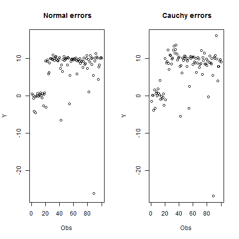
Figure 1: Model with normal and Cauchy errors, with one change-point in $l^{0}=20$, far parameters for the two phases.

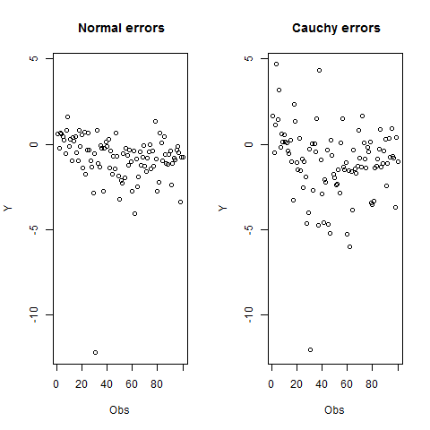
Figure 2: Model with normal and Cauchy errors, with one change-point in $l^{0}=20$, close parameters for the two phases.

4.2 Unknown change-point number

In view of these results, in order to study the selection criterion of the change-point number, we will consider only Normal and Cauchy distributions for errors. We simulate a model with one change-point in $l^{0}_{1}=20$ for $n=100$ observations. The estimation $\hat{K}^{(\tau)}_{n}$ of the change-point number associated to quantile method is calculated using Remark 3.3. For criterion (23), for the penalty we consider $P(K,p)=Kp$ and deterministic sequence $B_{n}=n^{5/8}$. The estimation of the change-point number associated to LS method, is the minimizer in $K$ of

$$n\log\left(n^{-1}\min_{(\textrm{$\mathbf{\theta}$}_{1},\textrm{$\mathbf{\theta}$}_{2})}\left\{\sum^{K}_{r=1}\sum^{l_{r}}_{i=l_{r-1}+1}\left[Y_{i}-g(\textrm{$\mathbf{X}$}_{i},\textrm{$\mathbf{\phi}$}_{r})\right]^{2}\right\}\right)+P(K,p)B_{n}.$$

Two cases are considered for the true regression parameters: the parameters of the two (true) phases are far (Figure 2), $\textrm{$\mathbf{\phi}$}^{0}_{1}=(0.5,1)$, $\textrm{$\mathbf{\phi}$}^{0}_{2}=(10,2.5)$ and the parameters are closely (Figure 2), $\textrm{$\mathbf{\phi}$}^{0}_{1}=(0.5,1)$, $\textrm{$\mathbf{\phi}$}^{0}_{2}=(1,-0.5)$. In the case of Gaussian errors, the criterion associated to the LS method is slightly better when the parameters are far. The criteria associated to the two methods (LS and quantile) give the same good results if the parameters are closely. In the case of Cauchy errors, the quantile criterion selects well the change-point number when the parameters are far, while when the parameters are closely, the two criteria rather prefer a model without change-points (Tables 4).

4.3 Conclusion

These simulations allow us to conclude that for a nonlinear model with change-points, when the errors are Gaussian, the quantile method, proposed in this paper, gives similar results to those obtained by least squares method. On the other hand, for heavy-tailed errors, the performance of the quantile method is better than LS method, whether in estimation or in selection criterion.

Appendix A Bernstein’s Inequality

Bernstein’s Inequality (see for example Pollard (1984)).
Let $Z_{i}$ be a sequence of independent random variables with mean zero and $|Z_{i}|\leq\beta$ for some $\beta>0$. Let also $V\geq\sum^{n}_{i=1}I\!\!E[Z_{i}^{2}]$. Then for all $0<s<1$ and $0\leq z\leq V/(s\beta)$, we have

$$I\!\!P\left[|\sum^{n}_{i=1}Z_{i}|>z\right]\leq 2\exp\left(-z^{2}s(1-s)/V\right).$$ (24)

References

- Bai (1998) Bai, J., Estimation of multiple-regime regressions with least absolute deviation. Journal of Statistical Planning Inference, 74, 103-134, (1998).
- Bai and Perron (1998) Bai, J., Perron P., Estimating and testing linear models with multiple structural changes, Econometrica 66(1), 47-78, (1998).
- Boldea and Hall (2013) Boldea, O., Hall, A.R., Estimation and inference in unstable nonlinear least squares models. Journal of Econometrics, 172(1), 158-167, (2013).
- Chen et al. (2013) Chen L.A., Tran L.T., Lin L.C., Symmetric regression quantile and its application to robust estimation for the nonlinear regression model, Journal of Statistical Planning and Inference, 126(2), 423-440, (2004).
- Choi et al. (2005) Choi S.H., Kim K.J., Lee M.S., Robust test based on nonlinear regression quantile estimators, Communications of the Korean Mathematical Society, 20(1), 145-159, (2005).
- Ciuperca (2009) Ciuperca G., The M-estimation in a multi-phase random nonlinear model. Statistics and Probability Letters, 75(5), 573-580, (2009).
- Ciuperca (2011a) Ciuperca, G., A general criterion to determinate the number of change-points. Statistics and Probability Letters, 81, no 8, 1267-1275, (2011).
- Ciuperca (2011b) Ciuperca G., Estimating nonlinear regression with and without change-points by the LAD-method. Annals of the Institute of Statistical Mathematics, 63(4), 717-743, (2011).
- Ciuperca (2014) Ciuperca G., Adaptive model selection in a high-dimension multiphase quantile regression. arXiv:1309:1262, (2014).
- Furno (2012) Furno M., Tests for structural break in quantile regressions. AStA Advances in Statistical Analysis, 96(4), 493-515, (2012).
- Knight (1998) Knight K., Limiting distributions for regression estimators under general conditions, Annals of Statistics, 26(2), 755-770, (1998).
- Koenker (2005) Koenker R., Quantiles regression, Econometric Society Monographs, No 38, Cambridge University Press, (2005).
- Koenker and Bassett (1978) Koenker R., Bassett G., Regression Quantiles, Econometrica, 46, 33-50, (1978).
- Koul and Qian (2002) Koul, H.L., Qian, L., Asymptotics of maximum likelihood estimator in a two-phase linear regression model. Journal of Statitical Planning and Inference 108, 99-119, (2002).
- Koul et al. (2003) Koul, H.L., Qian, L., Surgailis, D., Asymptotics of M-estimators in two-phase linear regression models. Stochastic Processes and their Applications 103, 123-154, (2003).
- Oberhofer (1982) Oberhofer W., The consistency of nonlinear regression minimizing the L1-norm. Annals of Statistics, 10(1), 316-319, (1982).
-
Oberhofer and Haupt (2014)
Oberhofer W., Haupt H.,
Asymptotic theory for nonlinear quantile regression under weak dependence.
Working Paper. https://www.researchgate.net/publication/29858831_Asymptotic_theory_for_nonlinear
_quantile_regression_under_weak_dependence, (2014). - Oka and Qu (2011) Oka T., Qu Z., Estimating structural changes in regression quantiles. Journal of Econometrics, 162, 248-267, (2011).
- Pollard (1984) Pollard D., Convergence of stochastic processes, Springer, New York, (1984).
- Qu (2008) Qu Z., Testing for structural change in regression quantiles. Journal of Econometrics, 146, 170-184, (2008).
- Seber and Wild (2003) Seber, G.A.F., Wild, C.J., Nonlinear regression. Wiley Series in Probability and Statistics, New Jersey, (2003).
- van der Vaart and Wellner (1996) van der Vaart A.W., Wellner J.A.,. Weak convergence and empirical processes. With applications to statistics, Springer Series in Statistics, New York, (1996).