Kane-Mele Hubbard model on a zigzag ribbon: stability of the topological edge states and quantum phase transitions

Abstract

We study the quantum phases and phase transitions of the Kane-Mele Hubbard (KMH) model on a zigzag ribbon of honeycomb lattice at a finite size via the weak-coupling renormalization group (RG) approach. In the non-interacting limit, the KM model is known to support topological edge states where electrons show helical property with orientations of the spin and momentum being locked. The effective inter-edge hopping terms are generated due to finite-size effect. In the presence of an on-site Coulomb repulsive interaction and the inter-edge hoppings, special focus is put on the stability of the topological edge states (TI phase) in the KMH model against (i) the charge and spin gaped (II) phase, (ii) the charge gaped but spin gapless (IC) phase and (iii) the spin gaped but charge gapless (CI) phase depending on the number (even/odd) of the zigzag ribbons, doping level (electron filling factor) and the ratio of the Coulomb interaction to the inter-edge tunneling. We discuss different phase diagrams for even and odd numbers of zigzag ribbons. We find the TI-CI, II-IC, and II-CI quantum phase transitions are of the Kosterlitz-Thouless (KT) type. By computing various correlation functions, we further analyze the nature and leading instabilities of these phases.

I Introduction.

Recently, there has been growing interest in topological insulators (TIs) and superconductors which support gapless edge (surface) states while the bulk remains insulating Kane-review ; SCZhang-review . These surface states come as a consequence of the spin-orbit (SO) couplings, and are protected by the time-reversal symmetry (TRS)Kane-review ; SCZhang-review . The topological nature of TIs lies in the non-trivial topological $Z_{2}$ invariantKM while it becomes trivial for an ordinary band insulator (BI). The theoretical predictionsSCZhang-science2006 ; Fu-Kane-2007 ; chinese-SCZhang of TIs have been soon observed experimentally in various insulators with strong SO couplingsTI-exp . In two-dimensional systems, these topological states have been predicted in the framework of the quantum spin Hall insulator (QSHI)Haldane ; KM ; KM2 ; bernevig1 ; Fu ; bernevig2 , and have been realized experimentally soon after in $HgTe/CdTe$ quantum well structuresSCZhang-science2006 . Unlike the integer quantum Hall where the chiral (one propagating mode of electrons with a single spin species) edge states are generated by an external magnetic field which breaks TRS, the TRS preserving QSHI systems lead to helical edge states in the absence of a magnetic field in which propagation direction at one edge is opposite for opposite spinsbernevig2 . This one-dimensional helical edge state electrons are protected by TRSKM and are free of spin-flip backscatteringsSCZhang-review . As a result, they lead to perfect transmission in charge transport along the edgeSCZhang-physicstoday .

A simple theoretical model was first introduced by HaldaneHaldane and later proposed by Kane and MeleKM ; KM2 (the KM model) to capture the helical edge states of QSHIs. The KM model was aimed to describe edge states in graphene. Though the SO coupling in graphene is expected to be too small to observe the edge states, the KM Model is regarded as a generic model for 2D TIs. The existence of the helical edge states in KM model has been well studied. Recently, more attention has been put on the stability, exotic quantum phases and phase transitions of the helical edge states and possible exotic quantum phases in the correlated Kane-Mele HubbardMeng ; hur ; assaad ; sandler ; GMZhang model upon including the on-site Coulomb repulsions (the Hubbard $U$ term) in the KM model. In a pioneering work by Meng et al. in Ref.  Meng, via Quantum Monte Carlo and dynamical mean-field approaches, the helical edge states are stable up to a finite Hubbard interaction, and a gaped spin-liquid phase was predicted in the phase diagram of the KM Hubbard model at half filling for small to intermediate range of $U$. Moreover, the 1D Luttinger liquid physics with power-law correlations for the helical edge states has been studied numericallyassaad as well as analyticallybena in the framework of the KM Hubbard model. Meanwhile, the doping effect on the KM Hubbard model was addressed in Ref. fiete, where spin liquid phase was argued to become superconducting state.

In this paper, we present a theoretical analysis on the KM Hubbard model at half filling and away from half filling from a different perspective: we analyze the model on a finite-sized zigzag ribbon (where the helical edge states have been realized numerically in the tight-binding KM modelhur ) with a ribbon width $L=(N-1)b$ ($N$ being the number of zigzag chain in a ribbon and $b$ is defined in Fig. 1) in the weak-coupling (weak on-site Coulomb $U$) limit via perturbative renormalization group (RG) combined with the bosonization approaches. Note that one can alternatively study the model on an armchair ribbon, which was suggested to support edge states in graphene (equivalent to the KM model without SO coupling)armchair . The authors in Ref. sandler, have studied the effects of long-range Coulomb interactions on the edge states of a finite-sized zigzag KM ribbon. The effects of the short-ranged electron-electron interaction on the helical edge states of the KM model have been addressed in Ref. Teo, . We shall emphasize here the stability of the helical edge states against the combined short-ranged on-site Coulomb interaction the and finite size effects, as well as possible other emerged quantum phases and phase transitions (QPTs)QPT among them.

The finite-size effect manifests itself in the structure of the energy spectrum and in an effective inter-edge tunneling terms. We further find that these behaviors for even number of zigzag KM ribbons ($N=even$) are different from those for $N=odd$. For $N=even$, a finite energy gap is found at half filling where the Fermi energy is at the Dirac point $ka=\pi$. This small gap is due to breaking of the sublattice translational invariance at the boundaries, and can be explained in terms of an effective finite single-particle inter-edge tunneling, which decays exponentially with increasing $L$. Away form half filling, the energy dispersion becomes gapless at the Fermi level. For $N=odd$, however, the energy spectrum is gapless and the single-particle inter-edge tunneling vanishes for both half filling and away from half filling. Nevertheless, for both $N=even$ and $N=odd$, two-particle processes, effective inter-edge two-particle spin-flip and inter-edge Umklapp (two-particle backscattering) terms, are generated via second-order inter-edge hoppings.

Our stability analysis of the KMH ribbon is summarized as follows. For $N=even$, the energy gap at half-filled at the Dirac point gives rise to a charge and spin gaped (insulating) (II) phaseTeo ; at a generic filling, however, the two-particle processes when combined with the effect of the Hubbard $U$ term lead to the instabilities of the helical edge states towards a charge gapless but spin gaped (CI) phaseTeo in the RG analysis via the Kosterlitz-Thouless type of quantum phase transitions. When $L\rightarrow\infty$, the inter-edge hopping term vanishes, the TI phase at half filling is unstable against the charge gaped but spin gapless (IC) phaseTeo for arbitrary $U>0$, while it is stable away from half filling. For $N=odd$, the single-particle inter-edge tunneling is absent, while the combined two-particle inter-edge hoppings and the on-site Coulomb repulsions make the TI unstable for any finite $U$ or inter-edge tunneling. As a result, the TI phase moves towards CI or IC or II phase depending on the ratio of Coulomb interaction and the inter-edge tunneling. The phase transitions for II-IC and II-CI are of the KT type.

By computing various correlation functions, we further analyze the instabilities of the helical edge states, the CI and IC phases towards the charge-density-wave (CDW), spin-density-wave (SDW) as well as the singlet (SS) and triplet (TT) superconducting states.

The remaining parts of the paper is organized as follows. In Sec. II, the Kane-Mele Hubbard at a finite size is introduced. The model is re-expressed in terms of the scalar and vector current operators. In Sec. III, the stability of the helical edge states is addressed via weak-coupling RG analysis. We also address the nature of the quantum phase transitions between the TI and other quantum phases. We conclude in Sec. IV.

II Model Hamiltonian.

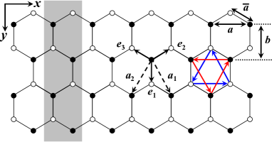
Figure 1: (Color online) Honeycomb lattice of a finite-sized zigzag ribbon of the tight-binding Kane-Mele model with the ribbon size $N=4$ ($N$ being the number of zigzag chains along $x-$axis) along $y-$axis. The honeycomb lattice consists of two inter-penetrating triangular lattices denoted by sublattice $A$ (dark circles) and sublattice $B$ (open circles) with lattice vectors ${\bf a_{1}}$ and ${\bf a_{2}}$ (dashed arrows). The zigzag ribbon shows translational symmetry along $x-$axis. The nearest-neighbor lattice vectors between nearest-neighbor $A$ and $B$ sites are denoted by ${\bf e_{i=1,2,3}}$ with a lattice constant $a$. The red (black) arrows within sublattice $A(B)$ represent the directions of the next-nearest-neighbor hopping term $\lambda_{SO}$ in the KM model (see text). The gray shaded region represents for the super-unit-cell of the zigzag ribbon, which repeats itself along $x-$axis.

II.1 The non-interacting Kane-Mele zigzag ribbon

Before we study the interacting Kane-Mele Hubbard model, it is worthwhile summarizing the main results for the non-interacting Kane-Mele (KM) model on a zigzag ribbon of honeycomb lattice, given by the following HamiltonianKM :

$$H_{KM} = -t\sum\limits_{\left\langle{ij}\right\rangle,\sigma}{c_{i\sigma}^{\dagger}c_{j\sigma}}+i\lambda_{SO}\sum\limits_{\left\langle{\left\langle{ij}\right\rangle}\right\rangle,\sigma}{\nu_{ij}c_{i\sigma}^{\dagger}s^{z}c_{j\sigma}}+h.c.$$

where $\left\langle i,j\right\rangle$ and $\left\langle\left\langle i,j\right\rangle\right\rangle$ refer to the nearest-neighbor (NN) and next-nearest-neighbor (NNN) sites, respectively. The NN and NNN lattice vectors for the honeycomb lattice are denoted respectively by ${\bf e_{i=1,2,3}}$ and ${\bf a_{i=1,2}}$hur :

$${\bf e_{1}} = \bar{a}(0,1),{\bf e_{2}}=\bar{a}/2(\sqrt{3},-1),{\bf e_{3}}=\bar{a}/2(-\sqrt{3},-1),$$

$${\bf a_{1}} = \bar{a}/2(\sqrt{3},3),{\bf a_{2}}=\bar{a}/2(-\sqrt{3},3)$$ (2)

with $\bar{a}$ being the lattice constant between nearest-neighbor $A$ and $B$. The spin-orbit coupling term is represented by the imaginary NNN hopping $\lambda_{SO}$ term within the same sublattice where $\nu_{ij}=1$ for ${i,j}\in A$ (red counterclockwise arrows in Fig. 1) and $\nu_{ij}=-1$ for ${i,j}\in B$ (blue clockwise arrows in Fig. 1).

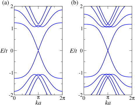
Figure 2: (Color online) Energy spectrum of a finite-sized Kane-Mele model on a zigzag ribbon for (a) $N=4$, (b) $N=5$ of honeycomb lattice. Here, we set $t=1$, $\lambda_{SO}/t=0.2$.

In the absence of the SO coupling, the KM model on zigzag ribbon reduces to the tight-binding Hamiltonian of a 2D zigzag graphene nano-ribbon (ZGNR)kyoko , which shows two in-equivalent Dirac points located at $k\equiv k_{x}=\pm\frac{2\pi}{3a}$ with $k_{x}$ being momentum along $x-$axis with $a\equiv\sqrt{3}\bar{a}$. Meanwhile, there exists a zero-energy flat band extended in the interval of $2\pi/3\leq ka\leq 4\pi/3$, known to correspond to the edge state of ZGNRkyoko ; fujita . It has been shown that the magnitudes of the edge state wave functions decay exponentially with distance away from the two edges, and the edge states are completely localized at the edges for $ka=\pi$fertig ; louie .

In the presence of SO couping, the KM Hamiltonian $H_{KM}$ for a finite-sized zigzag ribbon (see Fig. 1) on honeycomb lattice supports helical edge states $\Psi_{R,1(2)}^{\uparrow(\downarrow)},\Psi_{L,1(2)}^{\downarrow(\uparrow)}$ with topological natureKM ; hur . Here, $\Psi_{R,1(2)}^{\uparrow(\downarrow)}$ stands for the wave function of the right-moving edge state electron with spin up (spin down) along the edge $1$ ($2$), respectively. The indices $1$ and $2$ also refer to the top and bottom edge, respectively. Similarly, $\Psi_{L,1(2)}^{\downarrow\uparrow}$ stands for the the wave function of the left-moving edge state electron with spin down (spin up) along the edge $1$ ($2$), respectively. The helical nature of these topological edge states manifest itself in the lock-in between the electron spin configuration and the direction of its momentum.

In the limit of large ribbon size $N\gg 1$, the electron operator $c_{i}^{\sigma}(x)$ near the edge can be decomposed approximately in terms of these well-localized edge states as:

$$c_{1(2)}^{\uparrow(\downarrow)}(x) \approx \Psi_{R,1(2)}^{\uparrow(\downarrow)}(x)e^{{\it i}k_{F}x},$$

$$c_{1(2)}^{\downarrow(\uparrow)}(x) \approx \Psi_{L,1(2)}^{\downarrow(\uparrow)}(x)e^{-{\it i}k_{F}x}.$$ (3)

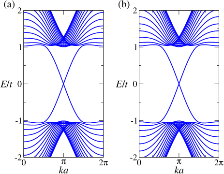
Figure 3: (Color online) Energy spectrum of a finite-sized Kane-Mele model on a zigzag ribbon for (a) $N=16$, (b) $N=15$ of honeycomb lattice. Here, we set $t=1$, $\lambda_{SO}/t=0.2$.

The Hamiltonian of the edge $H_{edge}$ is therefore given by:

$$H_{edge} = -{\it i}v_{F}\int dx[\Psi_{R,1}^{\dagger\uparrow}\partial_{x}\Psi_{R,1}^{\uparrow}-\Psi_{L,1}^{\dagger\downarrow}\partial_{x}\Psi_{L,1}^{\downarrow}$$ (4)

$$+ \Psi_{R,2}^{\dagger\downarrow}\partial_{x}\Psi_{R,2}^{\downarrow}-\Psi_{L,2}^{\dagger\uparrow}\partial_{x}\Psi_{L,2}^{\uparrow}]$$

with $v_{F}$ being the Fermi velocity.

At a finite system size, however, the edge state electron wave functions acquire an additional functional dependence on $y-$axis ($c_{1(2)}^{\uparrow(\downarrow)}(x,y)$) and are found to extend over a finite range in bulk via diagonalizing the tight-binding KM ribbon. The Hamiltonian of the edge states in this case are given by:

$$H_{edge} = v_{F}\int dk\int dyk[\bar{\Psi}_{R,1}^{\dagger\uparrow}(k,y)\bar{\Psi}_{R,1}^{\uparrow}(k,y)$$

$$- \bar{\Psi}_{L,1}^{\dagger\downarrow}(k,y)\bar{\Psi}_{L,2}^{\downarrow}(k,y)$$

$$+ \bar{\Psi}_{R,2}^{\dagger\downarrow}(k,y)\bar{\Psi}_{R,2}^{\downarrow}(k,y)-\bar{\Psi}_{L,2}^{\dagger\uparrow}(k,y)\bar{\Psi}_{L,2}^{\uparrow}(k,y)],$$

where $\bar{\Psi}_{R/L,1(2)}^{\uparrow(\downarrow)}(k,y)$ are the edge state electron operators for a KM ribbon at a given momentum $k$ and $y$ obtained via Fourier transforming $c_{1(2)}^{\uparrow(\downarrow)}(x,y)$ along the $x-$axis:

$$\bar{\Psi}_{R,1(2)}^{\uparrow(\downarrow)}(k,y) = \int dxe^{-{\it i}kx}c_{1(2)}^{\uparrow(\downarrow)}(x,y),$$

$$\bar{\Psi}_{L,1(2)}^{\downarrow(\uparrow)}(k,y) = \int dxe^{-{\it i}kx}c_{1(2)}^{\downarrow(\uparrow)}(x,y).$$ (6)

Note that $\bar{\Psi}_{R/L,1(2)}^{\uparrow(\downarrow)}(k,y)$ can be obtained numerically as the eigenstates of the Dirac dispersed helical edge states via diagonalizing the finite-sized zigzag KM ribbon. As shown in Fig. 2 and Fig. 3, we numerically diagonalize the KM model at $N=even$ ($N=4,16$) and $N=odd$ ($N=5,15$) zigzag ribbonhur ; van . Two pairs of Dirac dispersed edge states ($\bar{\Psi}_{R,1(2)}^{\uparrow(\downarrow)},\bar{\Psi}_{L,1(2)}^{\downarrow(\uparrow)}$) emerge in the energy spectrum of a finite-sized KM zigzag ribbon, and they tend to intersect at the Dirac points $ka=\pm\pi$. However, at the Dirac points, a finite energy gap is developed for $N=even$, while no gap is seen for all $N=odd$ (see Fig. 2). We shall focus on this even-odd effect in more details below. Similar to the case for ZGNR, for $2\pi/3\leq ka\leq 4\pi/3$, we find the square magnitude of the two degenerate edge state eigenfunctions $|\Psi(y)|^{2}=|\bar{\Psi}_{L/R,i}(k,y)|^{2}$ (except for $N=even$ and $ka=\pm\pi$) show a symmetrical exponential decay from one edge to the other with respect to the ribbon center ($y=L/2$) from both edges into the bulk as a function of the distance to the corresponding edge. Here, $y$ measures the distance to the edge along $y-$axis and $y=0$ corresponds to the first (top) zigzag chain. Also, to simplify the discussions, we use an integer index $y/b+1=N_{i}=1,2,\cdots N$ with $y=(N_{i}-1)b$ for labeling the $N_{i}$-th zigzag chain along $y-$axis for a ribbon with $N$ zigzag chains; $y=2b$ corresponds to the position of the third ($N_{i}=3$) zigzag chain. As shown in Fig. 4 (b) and Fig. 5, the decay of these edge states is well fitted by the following exponential form:

$$|\bar{\Psi}_{L/R,i}(k,y)|^{2}\propto e^{-\beta y/b}$$ (7)

where $\beta$ is the decay constant depends on the momentum $k$. For $N=even$ and at the Dirac point $ka=\pi$, we find the right and left moving edge states get hybridized so that the square magnitudes $|\Psi(y)|^{2}=|\bar{\Psi}_{hy,i}(y)|^{2}$ of the two degenerate edge states are maximized on both edges (see Fig. 4 (a)). Note that we find via eigenvector analysis of our numerical results through exact diagonalization of the finite-sized KM ribbon that these distinct two hybridized edge state wave-functions :$\bar{\Psi}_{hy,1}(y)\neq\bar{\Psi}_{hy,2}(y)$ show the same magnitudes: $|\bar{\Psi}_{hy,1}(y)|=|\bar{\Psi}_{hy,2}(y)|$. Numerically, the values of $|\Psi(y)|^{2}$ as a function of $y$ for a given edge state are obtained approximately by summing over the square of the matrix elements of the corresponding edge-state eigenvector contributed from both sublattices: $|\Psi(y)|^{2}=|\Psi_{A}(y)|^{2}+|\Psi_{B}(y+\bar{a}/2)|^{2}$. Also, we find the square magnitude $|\Psi(y)|^{2}$ at $ka=\pi$ for $N=even$ (see Fig. 4(a)) oscillate along $y-$axis. Similar oscillations are found for $N=odd$ but not shown in Fig. 5(a) as the values of $|\Psi(y)|^{2}$ for $N=odd$ near edges are vanishingly small and go beyond the logarithmic scale shown there. This oscillatory behavior agrees qualitatively with that shown in Ref. sandler, .

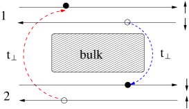
Figure 6: (Color online) Schematic diagram for the inter-edge hopping term $t_{\perp}$ (red or blue dashed line).

Based on our numerical results, the edge states are much more localized at the Dirac point $ka=\pm\pi$: $\beta(k=\pi/a)>1$ compared to that at other values of $k$. For $2\pi/3<ka<\pi$, however, the edge state wave functions extend over a finite region in the bulk (see Fig. 4 (b)). In both cases, a weak but finite overlap between edge and bulk electron wave functions is expected to be present in the zigzag KM ribbon, which generates an effective inter-edge hoping $t_{\perp}$ term approximately as (see Fig. 6 and Sec. II B):

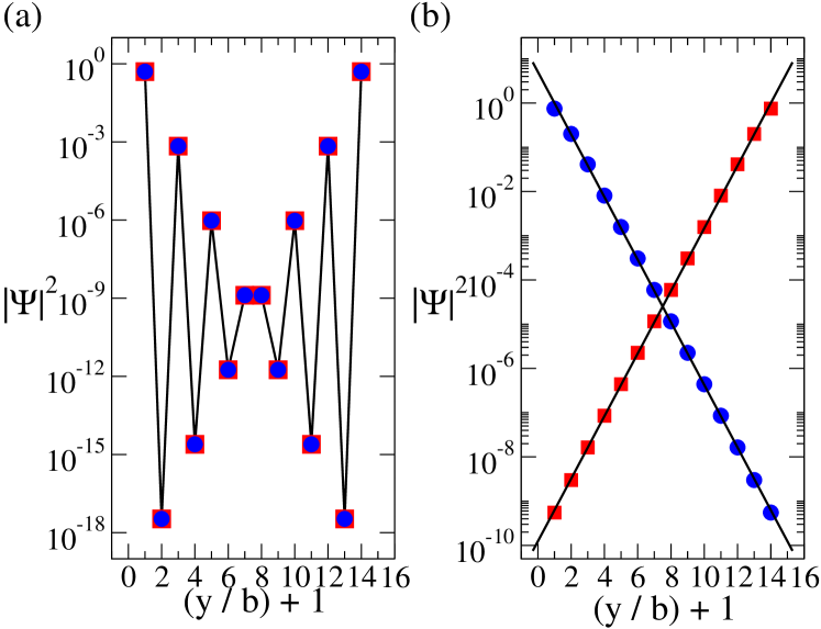
Figure 4: (Color online) The square magnitude of the edge state wave function $|\Psi|^{2}$ of the KM zigzag ribbon at half filling as a function of $y/b+1$ (defined in text) for $N=14$ and (a) for $ka=\pi$ and (b) for $ka=\pi\pm 0.2\pi$. Here, $|\Psi|^{2}$ (blue circles and red squares) represents for the square magnitude of the two edge state wave functions, which are degenerate eigenstates at the corresponding wave vector $k$. In (a), the two hybridized degenerate edge state wave functions $\Psi=\Psi_{hyb,i=1,2}$ (red and blue symbols) lead to the same square magnitude, $|\Psi_{hyb,1}|^{2}=|\Psi_{hyb,2}|^{2}$, in (b), we make the following identifications: $\Psi(y)=\Psi_{R,1}^{\uparrow}$ (blue) and $\Psi(y)=\Psi_{L,2}^{\uparrow}$ (red). The solid lines are guides to the eyes in (a), and in (b) they are fits to the exponential form in Eq. (7). We set $\lambda/t=0.1$.

$$H_{t_{\perp}} = t_{\perp}\sum_{\sigma=\uparrow,\downarrow}\int dx[c^{\dagger\sigma}_{1}c_{2}^{\sigma}+h.c.]$$

$$\approx t_{\perp}\int dxe^{2{\it i}k_{F}x}\left(\Psi_{R,1}^{\dagger\uparrow}\Psi_{L,2}^{\uparrow}+\Psi_{R,2}^{\dagger\downarrow}\Psi_{L,1}^{\downarrow}\right)+h.c..$$

with $x=na$ and $n=\pm 1,\pm 2,\cdots$. The value of $t_{\perp}$ in Eq. (LABEL:tperp) can be estimated numerically via diagonalizing the finite-sized KM ribbon:

$$H_{t_{\perp}} = t_{\perp}\sum_{\sigma=\uparrow,\downarrow}\int dx\int dy[c^{\dagger\sigma}_{1}(x,y)c_{2}^{\sigma}(x,y)+h.c.]$$

$$\approx t_{\perp}\int dy[\bar{\Psi}_{R,1}^{\dagger\uparrow}(k_{F},y)\bar{\Psi}_{L,2}^{\uparrow}(k_{F},y)$$

$$+ \bar{\Psi}_{R,2}^{\dagger\downarrow}(k_{F},y)\bar{\Psi}_{L,1}^{\downarrow}(k_{F},y)]+h.c..$$

The $H_{t_{\perp}}$ turns out to be important in our RG analysis on the stability of the helical edge states (see below). The magnitude of $t_{\perp}$ can be estimated via the overlap integralmermin of the opposite edge state wave functions through exact diagonalization of the tight-binding KM model at a finite-sized ribbon (see Eq. (LABEL:tperp-ribbon))der-hau-lee :

$$t_{\perp}\approx t\int_{0}^{L}dy[\bar{\Psi}_{R,1}^{\ast\uparrow}(y)\bar{\Psi}_{L,2}^{\uparrow}(y)+\bar{\Psi}_{L,1}^{\ast\downarrow}(y)\bar{\Psi}_{R,2}^{\downarrow}(y)+c.c.],$$ (10)

where we have dropped the $k_{F}$ dependence in $\bar{\Psi}_{L/R,\alpha}^{\sigma}(k_{F},y)$ in Eq. (10). At half filling, $k_{F}a=\pm\pi$, hence $e^{2{\it i}k_{F}x}=1$ and $H_{t_{\perp}}$ can in general survive. However, $N=even$ and $N=odd$ lead to different results in this case as explained below.

For $N=even$, due to breaking of the sublattice translational invariance at the boundaries results in a finite $t_{\perp}$. This leads to opening up a gap $\Delta$ in the excitation spectrum at the Dirac point when combining Eqs. (4) and (LABEL:tperp):

$$\epsilon(k-\pi/a) \approx \pm\sqrt{v_{F}^{2}(k-\pi/a)^{2}+(\Delta/2)^{2}}$$ (11)

with $\Delta=2t_{\perp}$. We numerically analyzed the gap $\Delta$ as shown in Fig. 7. The existence of a finite $t_{\perp}$ not only agrees with the energy gap at the Dirac point, it also explains the hybridization of the left and right moving edge states that we found in numerics as the eigenstates of the edge states in the presence of $t_{\perp}$ are linear combinations of left and right moving edge states. It is clear from Fig. 7(a) that the magnitude of the gap decreases with increasing the ribbon size $L$. In fact, it shows an exponential decay (see Fig. 7 (b)):

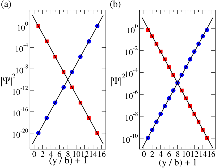
Figure 5: (Color online) The square magnitude of the edge state wave function $|\Psi|^{2}$ of the KM zigzag ribbon at half filling as a function of $y/b+1$ for (a) $N=15$ and $ka=\pi$ and (b) for $N=15$ and $ka=\pi\pm 0.2\pi$. Here, $|\Psi|^{2}$ (blue circles and red squares) represents for the square magnitude of the two edge state wave functions, which are degenerate eigenstates at the corresponding wave vector $k$. The solid lines are fits to the exponential form in Eq. (7). We set $\lambda/t=0.1$. Note that in (a) $|\Psi|^{2}$ is shown for only even values of $y/b$ (see text).

$$\Delta\approx\Delta_{0}e^{-\alpha L}$$ (12)

with $\alpha$ being the decay constant.

Note that the decay of the small gap $\Delta$ was found to be power-law fashion in Ref. sandler, by a different (analytical) approach based on the analytical eigenstates for KM model on 2D honeycomb lattice. With increasing $\lambda_{SO}$, we find the magnitude of $\Delta$ increases with increasing $\lambda_{SO}$, which comes as a result of the increase in bulk band gap $\Delta_{SO}$. We will show in Sec. IV. that this gaped phase corresponds to the charge and spin insulating (or II) phase. In the limit of infinite ribbon width $L\rightarrow\infty$, the gap $\Delta$ vanishes and the gapless Dirac spectrum is recovered. However, for $N=odd$, the sublattice translational symmetry at boundaries leads to cancellations in the overlap integral Eq. (10) between sublattices $A$ and $B$.

At a generic filling away from half-filled, the oscillatory phase factor $e^{2{\it i}k_{F}x}$ in $t_{\perp}$ term results in cancellations upon averaging over $x$ and $H_{t_{\perp}}$ hence vanishes. As shown below, we also numerically confirmed this result via Eq. (10). Though $H_{t_{\perp}}$ term survives only for $N=even$ and at half filling, as shown below, additional two-particle scattering terms are generated via second-order inter-edge tunnelings, which play an important role in all above-mentioned cases in our stability analysis of the helical edge states in KMH ribbon.

II.2 The Kane-Mele Hubbard model on a zigzag ribbon

Based on the above results for the non-interacting KM model on a finite-sized zigzag ribbon, we now perform an analytical analysis via perturbative RG approach on the weakly interacting KM model (the KM Hubbard model) by including a weak on-site Hubbard $U$ term in $H_{KM}$. Upon including the on-site Hubbard $U$ term, the Hamiltonian of the Kane-Mele-Hubbard (KMH) model reads:

$$H_{KMH} = H_{KM}+H_{U},$$

$$H_{U} = U\int dx\int dy[n^{\uparrow}(x,y)n^{\downarrow}(x,y)],$$

$$n^{\sigma}(x,y) = c^{\dagger\sigma}(x,y)c^{\sigma}(x,y)$$ (13)

with $U>0$. To simplify our calculations, we consider $H_{KM}$ approximately as three different contributions: (i) the well-localized edge state $H_{edge}$, (ii) the insulating bulk states $H_{b}$, and (iii) a weak coupling between edge and the bulk states $H_{t^{\prime}}$ due to the finite-size effect:

$$H_{KM}\approx H_{edge}+H_{b}+H_{t^{\prime}},$$ (14)

where the edge part $H_{edge}$ is defined in Eq. (4), the bulk part $H_{b}$ of $H_{KM}$ is given by:

$$H_{b} = \sum_{k,\alpha=\uparrow,\downarrow}H_{KM}(c_{b}^{\alpha}(k),c_{b}^{\dagger,\alpha}(k)),$$

(15)

and the edge-bulk overlap term $H_{t^{\prime}}$ reads:

$$H_{t^{\prime}} = t^{\prime}\int dx[e^{-{\it i}k_{F}x}\Psi_{R,1}^{\dagger\uparrow}c_{b,1}^{\uparrow}(x)+e^{{\it i}k_{F}x}\Psi_{L,1}^{\dagger\downarrow}c_{b,1}^{\downarrow}(x)$$

$$+ e^{-{\it i}k_{F}x}\Psi_{R,2}^{\dagger\downarrow}c_{b,2}^{\downarrow}(x)+e^{{\it i}k_{F}x}\Psi_{L,2}^{\dagger\uparrow}c_{b,2}^{\uparrow}(x)],$$

where $t^{\prime}\sim\mathcal{O}(t,\lambda_{SO})$.

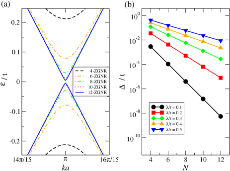
Figure 7: (Color online) (a) Energy spectrum $\epsilon$ versus momentum $k$ of the topological edge states of a finite-sized ($N$ zigzag chains) Kane-Mele model on a zigzag ribbon of honeycomb lattice near the Dirac point $ka=\pi$ for different ribbon sizes. Here, we set $t=1$, $\lambda_{SO}/t=0.5$. (b) Energy gap $\Delta$ at the Dirac point as a function of $N$ for different values of $\lambda$.

where $c_{b,1(2)}^{\sigma}(x)$ stands for the bulk electron operators near edge $1(2)$. We further simplify the Hubbard $U$ term $H_{U}$ in Eq. (13), and decompose it into the edge $H_{U,e}$ and the bulk $H_{U,b}$ contributions as:

$$H_{U} = H_{U,e}+H_{U,b},$$

$$H_{U,e} = U\int dx\sum_{i=1,2}[n_{i}^{\uparrow}(x)n_{i}^{\downarrow}(x)],$$

$$H_{U,b} = U\int dx\int dy[n_{b}^{\uparrow}(x,y)n_{b}^{\downarrow}(x,y)].$$ (17)

Here, $i=1(2)$ refers to the top (bottom) edge, $c_{b}^{\alpha}(k)$ is the electron destruction operator in the bulk. Also, the $H_{b}$ term, representing the KM model of the bulk electrons, shows an energy dispersion $E_{b}(k)$ with an energy gap $\Delta_{so}\sim 6\sqrt{3}\lambda_{SO}$hur . For the periodic 2D KM model, $E_{b}(k)$ has been shown to be (see Ref. hur, ):

$$E_{b}(k) = \pm\sqrt{|g_{k}|^{2}+\gamma_{k}^{2}},$$

$$g_{k} = t\sqrt{3+2\cos(\sqrt{3}k_{y})+4\cos(\sqrt{3}k_{y}/2)\cos(3k_{x}/2)},$$

$$\gamma_{k} = \lambda_{SO}[-\sin(\sqrt{3}k_{y})+2\cos(3k_{x}/2)\sin(\sqrt{3}k_{y}/2)].$$

To simplify our analysis, we assume here the bulk bands are well-separated by the bulk gap $\Delta_{SO}$ in the presence of a finite spin-orbit coupling $\lambda_{SO}$, and $U\ll\lambda_{SO}$. The on-site Hubbard $U$ term along the edges $H_{U,e}$ can be re-written as:

$$H_{U,e} = H_{\rho}+H_{\sigma}^{z},$$

$$H_{\rho} = g_{\rho}\int dxJ_{L}^{\rho}J_{R}^{\rho},$$

$$H_{\sigma}^{z} = g_{\sigma}^{z}\int dx\vec{J}_{L}^{z}\vec{J}_{R}^{z},$$

where $J^{\rho}_{R/L}$ is the $U(1)$ scalar current operator and $J^{z}_{L/R}$ is the $z-$component of the $SU(2)$ vector current operator $\vec{J}^{a=x,y,z}_{L(R)}$, defined respectively asgogolin ; giamarchi :

$$J^{\rho}_{L(R)} = \sum_{i=1,2}J^{\rho}_{L(R),i},$$

$$J^{\rho}_{L,1(2)} = \Psi_{L,1(2)}^{\dagger\downarrow(\uparrow)}\Psi_{L,1(2)}^{\downarrow(\uparrow)},$$

$$J^{\rho}_{R,1(2)} = \Psi_{R,1(2)}^{\dagger\uparrow(\downarrow)}\Psi_{R,1(2)}^{\uparrow(\downarrow)},$$

$$\vec{J}^{a=x,y,z}_{L(R)} = \Psi^{\dagger\alpha}_{L(R)}\vec{\sigma}^{a}_{\alpha\beta}\Psi_{L(R)}^{\beta},$$

$$\vec{J}_{L(R)}^{z} = \frac{1}{2}(\Psi_{L,2(R,1)}^{\dagger\uparrow}\Psi_{L,2(R,1)}^{\uparrow}-\Psi_{L,1(R,2)}^{\dagger\downarrow}\Psi_{L,1(R,2)}^{\downarrow}).$$

Here, $g_{\rho}$ and $g_{\sigma}^{z}$ take the following bare (initial) values in the context of renormalization group analysis: $g_{\rho}(\mu_{0})\equiv g_{\rho,0}=U/2$, $g_{\sigma}^{z}(\mu_{0})\equiv g_{\sigma}^{z,0}=-2U$ with $\mu_{0}$ being the bandwidth of the tight-binding KM model.

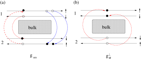
Figure 8: (Color online) Schematic diagrams for (a) the inter-edge Umklapp $g_{um}$ (red and blue arrows) and (b) the inter-edge spin-flip $g_{\sigma}^{\perp}$ processes.

We now turn our attention to $H_{t^{\prime}}$ term in Eq. (14). Integrating out the bulk electron $c_{b}^{\alpha}$ in Eqs. (15) and  (LABEL:Htprime), an effective inter-edge tunneling term $H_{t_{\perp}}$ as shown in Eq. (LABEL:tperp) is generated where $t_{\perp}\sim D_{bulk}(t^{\prime})^{2}/\Delta_{SO}$ with $D_{bulk}$ being the average electron density of states in the bulk. The estimation for $t_{\perp}$ here can be compared to that in Eq. (10) via numerical diagonalization of the KM ribbon. Note that the inter-edge hoping $t_{\perp}$ (or the bulk gap $\Delta_{SO}$) is enhanced with increasing spin-orbit coupling $\lambda_{SO}$: $t_{\perp}\propto(t^{\prime})^{2}/\Delta_{SO}\propto\lambda_{SO}^{2}/\Delta_{SO}\propto\lambda_{SO}$ (see Fig. 7(b)). Apart from $H_{t_{\perp}}$, the linear term in $t_{\perp}$, for both half filling and away from half filling cases, $H_{t_{\perp}}$ term will generate through the second order perturbation theory the following two two-particle scattering terms which turn out to be important in the stability analysis of topological edge states:

$$\tilde{H}_{t_{\perp}} = H_{um}+H_{\sigma}^{\perp},$$

$$H_{um} = g_{um}\int dx[e^{{\it i}4k_{F}x}[\Psi_{R,1}^{\dagger\uparrow}\Psi_{R,2}^{\dagger\downarrow}\Psi^{\uparrow}_{L,2}\Psi^{\downarrow}_{L,1}$$

$$+ \frac{1}{2}(\Psi_{R,1}^{\dagger\uparrow}(x)\Psi_{R,1}^{\dagger\uparrow}(x+a)\Psi^{\uparrow}_{L,2}(x)\Psi^{\uparrow}_{L,2}(x+a)$$

$$+ \Psi_{R,2}^{\dagger\downarrow}(x)\Psi_{R,2}^{\dagger\downarrow}(x+a)\Psi^{\downarrow}_{L,1}(x)\Psi^{\downarrow}_{L,1}(x+a))]+h.c.],$$

$$H_{\sigma}^{\perp} = g_{\sigma}^{\perp}\int dx(J_{L}^{+}J_{R}^{-}+h.c.),$$ (21)

where $H_{um}$ and $H_{\sigma}^{\perp}$ represent for the inter-edge Umklapp and inter-edge spin-flip terms, respectively (see Fig. 8), and the transverse components of the $SU(2)$ vector current operators $J^{+}_{L/R}$, $J^{-}_{L/R}$ are defined as:

$$J^{+}_{L(R)} \equiv \vec{J}_{L(R)}^{x}+{\it i}\vec{J}_{L(R)}^{y}=\Psi_{L,2(R,1)}^{\dagger\uparrow}\Psi_{L,1(R,2)}^{\downarrow},$$

$$J^{-}_{L(R)} \equiv \vec{J}_{L(R)}^{x}-{\it i}\vec{J}_{L(R)}^{y}=\Psi_{L,1(R,2)}^{\dagger\downarrow}\Psi_{L,2(R,1)}^{\uparrow},$$

Similar to Eq. (LABEL:tperp-ribbon), the bare couplings for $H_{\sigma}^{\perp}$ and $H_{um}$, $g_{um}(\mu_{0})\equiv g_{um}^{0}$ and $g_{\sigma}^{\perp}(\mu_{0})\equiv g_{\sigma}^{\perp,0}$ can be estimated numerically as:

$$g_{um}^{0} \approx \frac{t}{4}\int_{0}^{L}dy[\Psi_{R,1}^{\ast\uparrow}(y)\Psi_{R,2}^{\ast\downarrow}(y)\Psi^{\uparrow}_{L,2}(y)\Psi^{\downarrow}_{L,1}(y)$$

$$+ \frac{1}{2}(\Psi_{R,1}^{\ast\uparrow}(y)\Psi_{R,1}^{\ast\uparrow}(y)\Psi^{\uparrow}_{L,2}(y)\Psi^{\uparrow}_{L,2}(y)$$

$$+ \Psi_{R,2}^{\ast\downarrow}(y)\Psi_{R,2}^{\ast\downarrow}(y)\Psi^{\downarrow}_{L,1}(y)\Psi^{\downarrow}_{L,1}(y))+c.c],$$

$$g_{\sigma}^{\perp,0} \approx \frac{t}{2}\int_{0}^{y}dy[\Psi_{L,2}^{\ast\uparrow}(y)\Psi_{L,1}^{\downarrow}(y)\Psi^{\ast\downarrow}_{R,2}(y)\Psi^{\uparrow}_{R,1}(y)+c.c.].$$

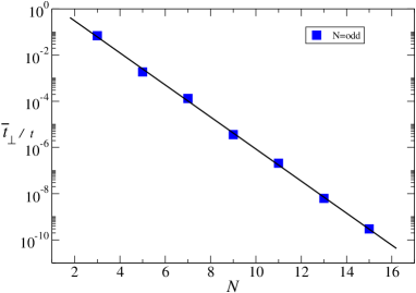
Figure 9: (Color online) The exponential decay of $\bar{t}_{\perp}$ as a function of odd number of zigzag chains $N$.

Note that the inter-edge Umklapp term $H_{um}$ depends sensitively on the electron filling factor. At half filling, $e^{{\it i}4k_{F}x}=1$, $H_{um}$ therefore in general survives. For $N=even$, we find $-g_{um}^{0}=g_{\sigma}^{\perp,0}=t_{\perp}^{2}/t$ via the energy gap $\Delta$ at the Dirac point. For $N=odd$, by substituting the edge state wave functions that we numerically obtained based on the tight-binding KM ribbon into Eq. (LABEL:bare-gum-gsigma), we find $-g_{um}^{0}=g_{\sigma}^{\perp,0}\equiv\bar{t}_{\perp}^{2}/t$, where

$$\bar{t}_{\perp}^{2}\approx t^{2}\int_{0}^{L}dy|\Psi_{R,1}^{\uparrow}(y)|^{2}|\Psi_{L,2}^{\uparrow}(y)|^{2}.$$ (24)

We further find numerically that $\bar{t}_{\perp}$ shows an exponential decay with increasing the ribbon width $L$, similar to the case for $N=even$:

$$\bar{t}_{\perp}\propto e^{-\gamma_{k}L}$$ (25)

with $\gamma_{k}$ being the decay constant (see Fig. 9). Note that at half filling, $\gamma_{k=\pi/a}\gg 1$ (or $t_{\perp}/t\ll 1$) due to the well-localized edge states.

When the system is away from half filling, however, the oscillatory factor $e^{{\it i}4k_{F}x}$ in $H_{um}$ leads to cancellations upon summing over $x$, and therefore $H_{um}$ term vanishes completely. Nevertheless, $H_{\sigma}^{\perp}$ term still survive: $g_{\sigma}^{\perp,0}\equiv\bar{t}_{\perp}^{2}/t$.

Note that similar two-particle scattering processes $H_{\sigma}^{\perp}$ and $H_{um}$ terms have been considered in Ref. Teo, in the context of the tunneling between helical edge states in a quantum point contact (QPC) as well as in Ref. fujimoto, . However, the authors in Ref. Teo, studied the effect of inter-edge single- and two-particle scattering processes on the helical edge states for a fixed electron-electron interactions (or Luttinger parameter $K$), while in Ref. fujimoto, the authors did not specify the origins of these two-particle scattering terms. By contrast, the two-particle scatterings we consider here come as a result of second-order inter-edge tunnelings. Furthermore, we treat the combined effects of the inter-edge two-particle scatterings $H_{\sigma}^{\perp}$, $H_{um}$ contributed from the inter-edge hopping $H_{t^{\perp}}$ as well as $H_{\rho}$, $H_{\sigma}^{z}$ terms via on-site Hubbard $U$ term in the weak-coupling limit on equal-footing.

Combining Eqs. (LABEL:H-U-edge)-(LABEL:J+-), the effective Hamiltonian of two weakly coupled helical edge states is therefore given by:

$$H^{eff}_{edge} = H_{edge}+H_{U,e}+\tilde{H}_{t_{\perp}}$$

$$= H_{edge}+H_{\sigma}^{\perp}+H_{\sigma}^{z}+H_{\rho}+H_{um}.$$

where $H_{edge}$ can be re-expressed in terms of the scalar and vector current operators as, similar to that for an one-dimensional non-interacting electrons at half fillinggogolin ; giamarchi :

$$H_{edge} = \int dx[\frac{\pi}{2}v_{F}^{c}\sum_{i=1,2}(J^{\rho}_{L,i}J_{L,i}^{\rho}+J^{\rho}_{R,i}J_{R,i}^{\rho})$$ (27)

$$+ \frac{2\pi}{3}v_{F}^{s}(\vec{J}_{L}\cdot\vec{J}_{L}+\vec{J}_{R}\cdot\vec{J}_{R})]$$

with the bare values for the Fermi velocities in the charge and spin sectors given by: $v_{F}^{c}=v_{F}^{s}=v_{F}$. Note that our effective Hamiltonian for the edges Eq. (LABEL:H_Hubbard) describes two weakly coupled helical Luttinger liquids. In particular, $H_{edge}$, describing two non-interacting helical edge states, exhibits $U(1)\times SU(2)$ symmetry; while as $H_{\sigma}^{\perp}+H_{\sigma}^{z}$ in the couplings between two edges break the $SU(2)$ spin rotational symmetry down to $Z_{2}$ symmetry. Our effective model for the weakly-coupled helical Luttinger liquids $H_{edge}$ can be characterized as one-dimensional fermionic Hubbard model with $SU(2)$ spin-anisotropic interactionshur ; gogolin ; giamarchi . The breaking of the $SU(2)$ symmetry of the model comes as a result of the Hubbard $U$ term at the edges (see Eq. (13)).

Figure 10: (Color online) Quantum phase diagram of the Kane-Mele Hubbard model at half filling for $N=even$ as a function of $U/t$ and $t_{\perp}^{2}/t$. The helical topological edge states (TI phase) is stable only at $U=t_{\perp}=0$ (dark circle). For a finite ribbon size, $t_{\perp}\neq 0$, the system flows to a charge and spin gaped (charge and spin insulating or II) phase.

III RG analysis and phase diagram of the KMH model.

We now analyze Eq.  (LABEL:H_Hubbard) via renormalization group approach the stability of the edge states in the presence of Hubbard interactions. Note that the Hamiltonian Eq. (LABEL:H_Hubbard) is closely related to the spin anisotropic Hubbard model for one-dimensional electrons where electron-electron interactions break the SU(2) symmetrygogolin ; giamarchi . Following the similar RG analysis to Refs. gogolin, ; giamarchi, , we may separate the four couplings $(g_{\rho},g_{um},g_{\sigma}^{\perp},g_{\sigma}^{z})$ into two pairs belonging to the spin sector $(g_{\sigma}^{z},g_{\sigma}^{\perp})$ and the charge sector $(g_{um},g_{\rho})$, respectively. Under RG transformations, these couplings exhibit the property of spin-charge separation, i.e. the renormalization of the couplings in the spin and charge sectors will remain in their own sector. We shall also analyze the single-particle inter-edge hopping $H_{t_{\perp}}$ term under RG. Below we separately discuss below the RG scaling equations for the half-filled and for a generic filling away from half filling for both $N=even$ and $N=odd$.

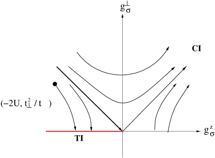
Figure 11: (Color online) The RG flows of the Kosterlitz-Touless type for the spin sector ($g_{\sigma}^{\perp},g_{\sigma}^{z}$) of the zigzag Kane-Mele Hubbard ribbon for $N=even$ away from half filling. The black circle stands for the initial (bare) couplings. The arrows indicate the directions of the RG flows upon decreasing the curt-off scale $\mu$ from $\mu_{0}$. The red line represents a line of fixed points in the TI phase, the TI-CI phase boundary is defined by the separatrix line (thick black arrow). Note that the coupling $g_{\rho}$ does not flow under RG in this case (see Eq. (LABEL:RG-c-doped)).

III.1 N=even

III.1.1 At half filling

As shown previously, at half filling ($k_{F}a=\pm\pi$), the KM model for a finite-sized zigzag ribbon induces a finite inter-edge hopping term, $t_{\perp}\neq 0$. It can be shown that under RG transformationgogolin , $H_{t_{\perp}}$ in Eq. (LABEL:tperp) is a relevant operator with scaling dimension $[t_{\perp}]=-1$. Hence, the RG scaling equation readsgogolin :

$$\frac{dt_{\perp}}{d\ln\mu}=-t_{\perp},$$ (28)

where $\mu$ is the running cutoff in energy. Under RG transformation, the running cutoff scale $\mu$ is lowered from $\mu_{0}>0$ to zero. It is clear that $t_{\perp}$ flows to a strong coupling fixed point, $t_{\perp}(\mu=0)=\infty$. As a result, both $g_{\sigma}^{\perp}$ and $g_{um}$ become relevant under RG as their magnitudes are proportional to $t_{\perp}^{2}$. When the two-particle spin-flip processes $g_{\sigma}^{\perp}$ term becomes relevant, a spin gap is opening up, while a charge gap develops when the two-particle backscattering $g_{um}$ term becomes relevant. Therefore, the $t_{\perp}\rightarrow\infty$ fixed point corresponds to the charge and spin gaped (or charge and spin insulating II) phase (see Fig. 10).

Figure 12: (Color online) Quantum phase diagram of the Kane-Mele Hubbard model away from half filling for $N=even$ as functions of $t_{\perp}^{2}/t$ and $U/t$. The helical topological edge states (TI phase) are unstable towards the charge conducting and spin insulating CI phase for $t_{\perp}^{2}/t>2U$. The TI-CI quantum phase transition set by the boundary $t_{\perp}^{2}/t=2U$ is of the Kosterlitz-Thouless (KT) type (red dashed arrows).

III.1.2 Away from half filling

We now proceed to address the case of finite doping away from half filling, $k_{F}a\neq\pi$. In this case, the inter-edge hopping term $H_{t_{\perp}}$ and Umklapp term $H_{um}$ vanish due to the oscillatory exponential factors $e^{2{\it i}k_{F}x}$ and $e^{4{\it i}k_{F}x}$ respectively (see Sec. II). The RG scaling equations for both finite-sized and infinite-sized ribbons are reduced togogolin ; giamarchi :

$$\frac{dg_{\rho}}{d\ln\mu} = 0,$$

in the charge sector with $g_{\rho}^{0}=U$ and

$$\frac{dg_{\sigma}^{\perp}}{d\ln\mu} = -g_{\sigma}^{\perp}g_{\sigma}^{z},$$

$$\frac{dg_{\sigma}^{z}}{d\ln\mu} = -(g_{\sigma}^{\perp})^{2},$$

in the spin sector with $(g_{\sigma}^{z,0},g_{\sigma}^{\perp,0})=(-2U,t_{\perp}^{2}/t)$.

Via Eq. (LABEL:RG-c-doped-even), it is clear that the system will not develop a charge gap under RG as $g_{\rho}$ does not diverge: $g_{\rho}(\mu)=g_{\rho}^{0}\ll 1$. The RG flows in the spin sector, however, suggest that the topological edge states may undergo the Kosterlitz-Thouless transition upon increasing $t_{\perp}$ to a charge gapless but spin gaped (CI) phase characterized by the following fixed point:

$$CI : g_{\sigma}^{\perp,0}+g_{\sigma}^{z,0}>0,g_{\sigma}^{z}(\mu\rightarrow 0),g_{\sigma}^{\perp}(\mu\rightarrow 0)\rightarrow\infty,$$

$$g_{\rho}(\mu\rightarrow 0)=0,g_{um}(\mu\rightarrow 0)=g_{um}^{0}\ll 1.$$

The TI-CI phase boundary is set by the separatrix $g_{\sigma}^{\perp}+g_{\sigma}^{z}=0$ (or when $t_{\perp}^{2}/t=2U$, see Fig. 11). The helical edge states are therefore stable for $t_{\perp}^{2}/t<2U$, while it is unstable against the CI phase for $U<\frac{t_{\perp}^{2}}{2t}$. Combing RG flows in both charge and spin sectors, this spin gaped phase corresponds to the charge conducting but spin insulating (or CI) phase (see Fig. 12).

III.2 N=odd

III.2.1 At half filling

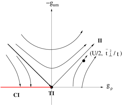
Figure 13: (Color online) The RG flows of the Kosterlitz-Touless type for the charge sector ($g_{\rho},g_{um}$) of the zigzag Kane-Mele Hubbard ribbon at half filling for $N=odd$. The black circle stands for the initial (bare) couplings at $(g_{\rho}^{0},-g_{um}^{0})=(U/2,\bar{t}_{\perp}^{2}/t)$. The arrows indicate the directions of the RG flows upon decreasing the curt-off scale $\mu$ from $\mu_{0}$. The red line represents a line of fixed points in the CI phase, the CI-II boundary is defined by the separatrix line (thick black arrow) and its quantum transition is of the Kosterlitz-Thouless (KT) type. The topological TI phase is stable only at the origin $U=0=\bar{t}_{\perp}$.

At half filling, $k_{F}a=\pm\pi$ and $t_{\perp}=0$, all the four couplings $(g_{\rho},g_{um},g_{\sigma}^{\perp},g_{\sigma}^{z})$ exist in general under RG transformations. Their initial (bare) couplings at $\mu=\mu_{0}$ are given by: $(g_{um}^{0},g_{\rho}^{0})=(-\bar{t}_{\perp}^{2}/t,U/2)$, $(g_{\sigma}^{z,0},g_{\sigma}^{\perp,0})=(-2U,\bar{t}_{\perp}^{2}/t)$. The RG scaling equations in this case can be casted in a spin-charge separated formgogolin ; giamarchi and are readily obtained via the operator product expansion (OPE) for the current algebra in the one-dimensional Hubbard model with broken $SU(2)$ symmetry (see, for example the Appendix in Chapter 17 of Ref. gogolin, ):

$$\frac{dg_{\rho}}{d\ln\mu} = -g_{um}^{2},$$

$$\frac{dg_{um}}{d\ln\mu} = -g_{um}g_{\rho},$$

in the charge sector and

$$\frac{dg_{\sigma}^{\perp}}{d\ln\mu} = -g_{\sigma}^{\perp}g_{\sigma}^{z},$$

$$\frac{dg_{\sigma}^{z}}{d\ln\mu} = -(g_{\sigma}^{\perp})^{2},$$

in the spin sector.

As shown in Figs. 13 and  14, the generic RG flows of Eqs. (LABEL:RG-c) and (LABEL:RG-s) are of the Kosterlitz-Thouless (KT) type. In the charge sector, the RG flows for $g_{um}$ and $g_{\rho}$ with the bare couplings $(g_{um}^{0},g_{\rho}^{0})=(-\bar{t}_{\perp}^{2}/t,U/2)$ are always towards either the strong-coupling charg and spin gaped II phase for $-2\bar{t}_{\perp}^{2}/t<U<\frac{1}{2}\bar{t}_{\perp}^{2}/t$ or towards the charge conducting and spin insulating CI phase for $U<-2\bar{t}_{\perp}^{2}/t$. Similarly, in the spin sector, the TI phase is unstable against either the II phase for $-g_{\sigma}^{z,0}<g_{\sigma}^{\perp,0}$ (ie. $\bar{t}_{\perp}^{2}/t>2U$) or against a charge gaped but spin gapless IC phase for $-g_{\sigma}^{z,0}>g_{\sigma}^{\perp,0}$ (ie. $\bar{t}_{\perp}^{2}/t<2U$) (see Fig. 14). Therefore, the TI phase is unstable against any infinitesmall $U\neq 0$ and $\bar{t}_{\perp}\neq 0$. The II-IC and II-CI quantum phase transitions are of the KT type. Combining the RG flows for both spin and charge sectors, we obtain the global phase diagram shown in Fig.  15 for $N=odd$ and at half filling:

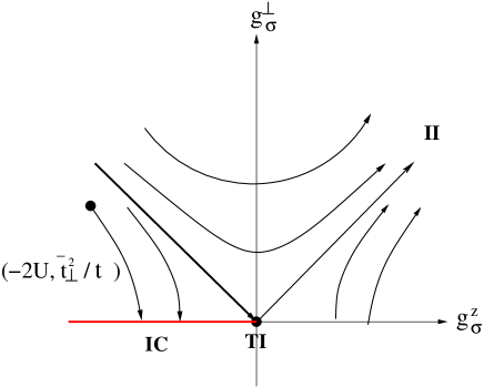
Figure 14: (Color online) The RG flows of the Kosterlitz-Touless type for the spin sector ($g_{\sigma}^{\perp},g_{\sigma}^{z}$) of the zigzag Kane-Mele Hubbard ribbon for $N=odd$ at half filling. The black circle stands for the initial (bare) couplings at $(g_{\sigma}^{z,0},g_{\sigma}^{\perp,0})=(-2U,\bar{t}_{\perp}^{2}/t)$. The arrows indicate the directions of the RG flows upon decreasing the curt-off scale $\mu$ from $\mu_{0}$. The red line represents a line of fixed points in the IC phase, the II-IC phase boundary is defined by the separatrix line (thick black arrow) and its quantum transition is of the Kosterlitz-Thouless (KT) type. The topological TI phase is stable only at the origin $U=0=\bar{t}_{\perp}$.

$$II : -2\bar{t}_{\perp}^{2}/t<U<\frac{1}{2}\bar{t}_{\perp}^{2}/t,$$

$$g_{\rho}(\mu\rightarrow 0),g_{um}(\mu\rightarrow 0)\rightarrow\infty,$$

$$\bar{t}_{\perp}^{2}/t>2U,g_{\sigma}^{z}(\mu\rightarrow 0),g_{\sigma}^{\perp}(\mu\rightarrow 0)\rightarrow\infty.$$

$$IC : U>\frac{1}{2}\bar{t}_{\perp}^{2}/t>0,$$

$$g_{\sigma}^{z}(\mu\rightarrow 0),g_{\sigma}^{\perp}(\mu\rightarrow 0)\rightarrow 0,$$

$$g_{\rho}(\mu\rightarrow 0),g_{um}(\mu\rightarrow 0)\rightarrow\infty.$$

$$CI : U<-2\bar{t}_{\perp}^{2}/t<0,$$

$$g_{\sigma}^{z}(\mu\rightarrow 0),g_{\sigma}^{\perp}(\mu\rightarrow 0)\rightarrow\infty,$$

$$g_{\rho}(\mu\rightarrow 0),g_{um}(\mu\rightarrow 0)\ll 1.$$

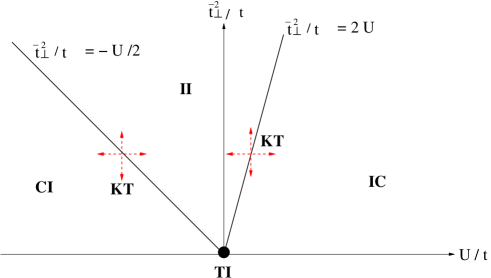
Figure 15: (Color online) Quantum phase diagram of the zigzag Kane-Mele Hubbard ribbon for $N=odd$ at half filling as a function of $U/t$ and $\bar{t}_{\perp}^{2}/t$. The helical topological edge states (TI) are unstable against any $U\neq 0$ or $\bar{t}_{\perp}\neq 0$, and towards the IC, CI and II phases for $U>\bar{t}_{\perp}^{2}/(2t)$, $U<-2\bar{t}_{\perp}^{2}/t$ and $-2\bar{t}_{\perp}^{2}/t<U<\frac{1}{2}\bar{t}_{\perp}^{2}/t$, respectively. The II-IC and II-CI phase transitions are of the Kosterlitz-Thouless (KT) type (red dashed arrows).

The topological edge states (TI) are unstable against the charge and spin insulating II phase for $-2\bar{t}_{\perp}^{2}/t<U<\frac{1}{2}\bar{t}_{\perp}^{2}/t$, against the charge insulating abd spin conducting IC phase for $U>\frac{1}{2}\bar{t}_{\perp}^{2}/t>0$, and against the charge conducting and spin insulating CI phase for $U<-2\bar{t}_{\perp}^{2}/t<0$. Therefore, TI phase is unstable for any $U\neq 0$ or $\bar{t}_{\perp}\neq 0$. The II-IC and II-CI quantum phase transitions are of the KT type. Our results on the stability of the TI phase for KM Hubbard model on a zigzag ribbon are different from those in Ref. Teo, through bosonizing the infinite-sized helical Luttinger liquid at a fixed interaction strength set by the Luttinger parameter $K=\sqrt{\frac{1-\frac{U}{2\pi v_{F}}}{1+\frac{U}{2\pi v_{F}}}}$. There, they showed that TI is stable for $1/2<K<2$. The difference lies in the fact that the inter-edge tunneling $t_{\perp}$ arised from the finite-size effect plays an important role here while it was absent in Ref. Teo, .

III.2.2 Away from half filling

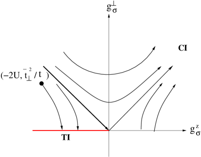
Figure 16: (Color online) The RG flows of the Kosterlitz-Touless type for the spin sector ($g_{\sigma}^{\perp},g_{\sigma}^{z}$) of the zigzag Kane-Mele Hubbard ribbon away from half filling for $N=odd$. The black circle stands for the initial (bare) couplings. The arrows indicate the directions of the RG flows upon decreasing the curt-off scale $\mu$ from $\mu_{0}$. The red line represents a line of fixed points in the TI phase, the TI-CI phase boundary is defined by the separatrix line (thick black arrow). Note that the coupling $g_{\rho}$ does not flow under RG in this case (see Eq. (LABEL:RG-c-doped)).

We now proceed to address the case of finite doping away from half filling, $k_{F}a\neq\pi$. In this case, the Umklapp term $H_{um}$ vanishes as mentioned in Sec. II. The RG scaling equations reduce to:

$$\frac{dg_{\rho}}{d\ln\mu} = 0,$$

in the charge sector with $g_{\rho}^{0}=U$ and

$$\frac{dg_{\sigma}^{\perp}}{d\ln\mu} = -g_{\sigma}^{\perp}g_{\sigma}^{z},$$

$$\frac{dg_{\sigma}^{z}}{d\ln\mu} = -(g_{\sigma}^{\perp})^{2},$$

in the spin sector with $(g_{\sigma}^{z,0},g_{\sigma}^{\perp,0})=(-2U,\bar{t}_{\perp}^{2}/t)$.

Via Eq. (LABEL:RG-c-doped), it is clear that the system will not develop a charge gap under RG as $g_{\rho}$ does not diverge: $g_{\rho}(\mu)=g_{\rho}^{0}\ll 1$. The RG flows in the spin sector (see Eq. LABEL:RG-s-doped), however, suggest that the topological edge states may undergo the Kosterlitz-Thouless transition upon increasing $\bar{t}_{\perp}$ to a spin gaped phase. Combing RG flows in both charge and spin sectors, this spin gaped phase corresponds to the charge conducting but spin insulating (or CI) phase (see Fig.  16). The TI-CI phase boundary is set by the separatrix $g_{\sigma}^{\perp}+g_{\sigma}^{z}=0$ (or when $\bar{t}_{\perp}^{2}/t=2U$, see Fig.  16). The helical edge states are therefore stable for $\bar{t}_{\perp}^{2}/t<2U$, while it is unstable against the CI phase for $U<\frac{\bar{t}_{\perp}^{2}}{2t}$ (see Fig. 17).

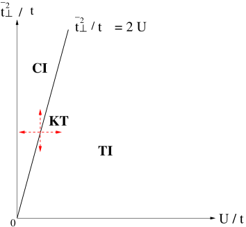
Figure 17: (Color online) Quantum phase diagram of the zigzag Kane-Mele Hubbard ribbon away from half filling for $N=odd$ as functions of $\bar{t}_{\perp}^{2}/t$ and $U/t$. The helical topological edge states (TI phase) are unstable towards the charge conducting and spin insulating CI phase for $\bar{t}_{\perp}^{2}/t>2U$. The TI-CI quantum phase transition set by the boundary $\bar{t}_{\perp}^{2}/t=2U$ is of the Kosterlitz-Thouless (KT) type (red dashed arrows).

IV Instabilities, orderings, and correlation functions of the Kane-Mele-Hubbard model

We now investigate further the nature of the TI, CI, IC and II phases. In particular, we focus on instabilities towards various orderings and correlation functions in these phases. Various correlation functions with specific orderings can be defined for this purpose: (i). the charge-density-wave $\mathcal{O}_{CDW}$ correlation, (ii). the spin-density-wave $\mathcal{O}_{SDW}^{a=x,y,z}$ correlation, (iii). the singlet $\mathcal{O}_{SS}$ and triplet $\mathcal{O}_{TS}^{a=x,y,z}$ superconducting pairing operators, wheregiamarchi

$$\mathcal{O}_{CDW} = \Psi^{\dagger\uparrow}_{R,1}(x)\Psi_{L,2}^{\uparrow}(x)+\Psi^{\dagger\downarrow}_{R,2}(x)\Psi_{L,1}^{\downarrow}(x),$$

$$\mathcal{O}_{SDW}^{x} = \Psi^{\dagger\uparrow}_{R,1}(x)\Psi_{L,1}^{\downarrow}(x)+\Psi^{\dagger\downarrow}_{R,2}(x)\Psi_{L,2}^{\uparrow}(x),$$

$$\mathcal{O}_{SDW}^{y} = -{\it i}[\Psi_{R,1}^{\dagger\uparrow}(x)\Psi_{L,1}^{\downarrow}(x)-\Psi^{\dagger\downarrow}_{R,2}(x)\Psi_{L,2}^{\uparrow}(x)],$$

$$\mathcal{O}_{SDW}^{z} = \Psi_{R,1}^{\dagger\uparrow}(x)\Psi_{L,2}^{\uparrow}(x)-\Psi^{\dagger\downarrow}_{R,2}(x)\Psi_{L,1}^{\downarrow}(x),$$

$$\mathcal{O}_{SS} = \Psi^{\dagger\uparrow}_{R,1}(x)\Psi_{L,1}^{\dagger\downarrow}(x)+\Psi^{\dagger\uparrow}_{L,2}(x)\Psi_{R,2}^{\dagger\downarrow}(x),$$

$$\mathcal{O}_{TS}^{x} = \Psi^{\dagger\uparrow}_{R,1}(x)\Psi_{L,2}^{\dagger\uparrow}(x)+\Psi^{\dagger\downarrow}_{L,1}(x)\Psi_{R,2}^{\dagger\downarrow}(x),$$

$$\mathcal{O}_{TS}^{y} = -{\it i}[\Psi_{R,1}^{\dagger\uparrow}(x)\Psi_{L,2}^{\dagger\uparrow}(x)-\Psi^{\dagger\downarrow}_{L,1}(x)\Psi_{R,2}^{\dagger\downarrow}(x)],$$

$$\mathcal{O}_{TS}^{z} = \Psi_{R,1}^{\dagger\uparrow}(x)\Psi_{L,1}^{\dagger\downarrow}(x)-\Psi^{\dagger\uparrow}_{L,2}(x)\Psi_{R,2}^{\dagger\downarrow}(x).$$

Note that some of the operators defined above involve helical electrons on both edges, different from those defined for a standard Luttinger liquid in one-dimensional interacting electrons where all electrons are along the same one-dimensional wiregogolin ; giamarchi . To investigate the above correlation functions, it is useful to bosonize the Hamiltonian Eq. (LABEL:H_Hubbard) asTeo :

$$H_{edge}^{eff} = \int dx[\sum_{\alpha=c,s}\frac{v_{\alpha}}{2}\left(K_{\alpha}(\partial_{x}\Theta_{\alpha})^{2}\!+\frac{1}{K_{\alpha}}(\partial_{x}\Phi_{\alpha})^{2}\right)$$

$$+ \frac{t_{\perp}}{2\pi a_{0}}\cos(\sqrt{2\pi}\Phi_{c}+2k_{F}x)\cos(\sqrt{4\pi}\Phi_{s})$$

$$+ \frac{g_{\sigma}^{\perp}}{(2\pi a_{0})^{2}}\cos(2\sqrt{2\pi}\Phi_{s})$$

$$+ \frac{1}{8\pi}\frac{g_{\sigma}^{z}}{(2\pi a_{0})^{2}}(\partial_{x}\Phi_{s}-\partial_{x}\Theta_{s})$$

$$+ \frac{g_{um}}{(2\pi a_{0})^{2}}\cos(2\sqrt{2\pi}\Phi_{c}+4k_{F}x)$$

$$+ \frac{1}{4}\frac{g_{\rho}}{(2\pi a_{0})^{2}}\sum_{\alpha=c,s}\left((\partial_{x}\Phi_{\alpha})^{2}-(\partial_{x}\Theta_{\alpha})^{2}\right)]$$

where via bosonization formulas,Teo ; gogolin ; giamarchi

$$\Psi_{L\sigma} = \frac{1}{\sqrt{2\pi a_{0}}}\eta_{\sigma}e^{-i\sqrt{4\pi}\phi_{L\sigma}}\ ,$$

$$\Psi_{R\sigma} = \frac{1}{\sqrt{2\pi a_{0}}}\eta_{\sigma}e^{i\sqrt{4\pi}\phi_{R\sigma}}\ ,$$

and the bosonic fields defined as:

$$\Phi_{\sigma} = \phi_{L\sigma}+\phi_{R\sigma}\ ,~{}~{}\Theta_{\sigma}=\phi_{L\sigma}-\phi_{R\sigma}\ ,$$

$$\Phi_{c(s)} = \frac{1}{\sqrt{2}}(\phi_{\uparrow}\pm\phi_{\downarrow})\ ,~{}~{}\Theta_{c(s)}=\frac{1}{\sqrt{2}}(\Theta_{\uparrow}\pm\Theta_{\downarrow}).$$

with $\eta_{\sigma}$ being the Klein factor and $a_{0}$ being the short-distance cutoff. In terms of these boson fields, the correlation functions mentioned above are given by:

$$\mathcal{O}_{CDW} = \frac{e^{-2{\it i}k_{F}x}}{\pi a_{0}}e^{-{\it i}\sqrt{2\pi}\Phi_{c}}\cos(\sqrt{2\pi}\Phi_{s}),$$

$$\mathcal{O}_{SDW}^{x} = \frac{e^{-2{\it i}k_{F}x}}{\pi a_{0}}e^{-{\it i}\sqrt{2\pi}\Phi_{c}}\cos(\sqrt{2\pi}\Theta_{s}),$$

$$\mathcal{O}_{SDW}^{y} = -\frac{e^{-2{\it i}k_{F}x}}{\pi a_{0}}e^{-{\it i}\sqrt{2\pi}\Phi_{c}}\sin(\sqrt{2\pi}\Theta_{s}),$$

$$\mathcal{O}_{SDW}^{z} = {\it{i}}\frac{e^{-2{\it i}k_{F}x}}{\pi a_{0}}e^{-{\it i}\sqrt{2\pi}\Phi_{c}}\sin(\sqrt{2\pi}\Phi_{s}),$$

$$\mathcal{O}_{SS} = \frac{1}{\pi a_{0}}e^{{\it i}\sqrt{2\pi}\Theta_{c}}\cos(\sqrt{2\pi}\Phi_{s}),$$

$$\mathcal{O}_{TS}^{x} = \frac{1}{\pi a_{0}}e^{{\it i}\sqrt{2\pi}\Theta_{c}}\cos(\sqrt{2\pi}\Theta_{s}),$$

$$\mathcal{O}_{TS}^{y} = -\frac{1}{\pi a_{0}}e^{{\it i}\sqrt{2\pi}\Theta_{c}}\sin(\sqrt{2\pi}\Theta_{s}),$$

$$\mathcal{O}_{TS}^{z} = \frac{1}{\pi a_{0}}e^{{\it i}\sqrt{2\pi}\Theta_{c}}\sin(\sqrt{2\pi}\Phi_{s}).$$

Based on the phase diagram via weak-coupling RG and the bosonized form of the Hamiltonian, we analyze below the instabilities and the behaviors of various correlation functions for (i) the charge and spin gapless (TI) topological edge states, (ii) the CI phase, (iii) the IC phase, and (iv) the II phase.

IV.0.1 The topological edge states (TI) phase

In the gapless topological edge states– the charge and spin conducting state–various correlation functions can be computed via correlation functions of the boson fields, given by:

$$<\mathcal{O}_{CDW}^{\dagger}(0)\mathcal{O}_{CDW}(r)> \sim e^{-2{\it i}k_{F}x}(\frac{1}{r})^{K_{c}+K_{s}}$$

$$\sim e^{-2{\it i}k_{F}x}(\frac{1}{r})^{1/K+K},$$

$$<\mathcal{O}_{SDW}^{\dagger x}(0)\mathcal{O}_{SDW}^{x}(r)> \sim e^{-2{\it i}k_{F}x}(\frac{1}{r})^{K_{c}+1/K_{s}}$$

$$\sim e^{-2{\it i}k_{F}x}(\frac{1}{r})^{2K},$$

$$<\mathcal{O}_{SDW}^{\dagger y}(0)\mathcal{O}_{SDW}^{y}(r)> \sim e^{-2{\it i}k_{F}x}(\frac{1}{r})^{K_{c}+1/K_{s}}$$

$$\sim e^{-2{\it i}k_{F}x}(\frac{1}{r})^{2K},$$

$$<\mathcal{O}_{SDW}^{\dagger z}(0)\mathcal{O}_{SDW}^{z}(r)> \sim e^{-2{\it i}k_{F}x}(\frac{1}{r})^{K_{c}+K_{s}}$$

$$\sim e^{-2{\it i}k_{F}x}(\frac{1}{r})^{1/K+K},$$

$$<\mathcal{O}_{SS}^{\dagger}(0)\mathcal{O}_{SS}(r)> \sim (\frac{1}{r})^{1/K_{c}+K_{s}}\sim(\frac{1}{r})^{2/K},$$

$$<\mathcal{O}_{TS}^{\dagger x}(0)\mathcal{O}_{TS}^{x}(r)> \sim (\frac{1}{r})^{1/K_{c}+1/K_{s}}\sim(\frac{1}{r})^{K+1/K},$$

$$<\mathcal{O}_{TS}^{\dagger y}(0)\mathcal{O}_{TS}^{y}(r)> \sim (\frac{1}{r})^{1/K_{c}+1/K_{s}}\sim(\frac{1}{r})^{1/K+K},$$

$$<\mathcal{O}_{TS}^{\dagger z}(0)\mathcal{O}_{TS}^{z}(r)> \sim (\frac{1}{r})^{1/K_{c}+K_{s}}\sim(\frac{1}{r})^{1/(2K)}$$

with $K_{c}=K$ and $K_{s}=1/K$ in the helical Luttinger liquidTeo . Note that in the conventional spinful Luttinger liquids where $K_{s}=1$, the above correlation functions get modified accordinglybena ; gogolin ; giamarchi .

IV.0.2 The CI phase

Now, we analyze instability and correlation functions in the the charge conducting and spin insulating (CI) phase. As shown in Eqs. (LABEL:CI) and (LABEL:H_bosonized), $g_{\sigma}^{\perp},g_{\sigma}^{z}\rightarrow\infty$ while $g_{\rho},g_{um}\rightarrow 0$ in this phase. In the bosonized form of the Hamiltonian, this implies that $\Phi_{s}$ is pinned to a constant valueTeo ; gogolin ; giamarchi : $\Phi_{s}\sim n\pi/\sqrt{8\pi}$. As a result, its conjugate variable $\Theta_{s}$ is disordered and exhibit exponentially decaying correlation functionsgogolin ; giamarchi . The corresponding leading correlation functions have the following power-law behaviors:

$$<\mathcal{O}_{CDW}^{\dagger}(0)\mathcal{O}_{CDW}(r)> \sim (\frac{1}{r})^{K_{c}}\sim(\frac{1}{r})^{K},$$

$$<\mathcal{O}_{SS}^{\dagger}(0)\mathcal{O}_{SS}(r)> \sim (\frac{1}{r})^{1/K_{c}}\sim(\frac{1}{r})^{1/K}.$$

Note that due to the disordered nature of the $\Theta_{s}$ field, the SDW as well as the TS orderings vanish: $<\mathcal{O}_{SDW}^{\dagger x,y,z}\mathcal{O}_{SDW}^{x,y,z}>\rightarrow 0,<\mathcal{O}_{TS}^{\dagger x,y,z}\mathcal{O}_{TS}^{x,y,z}>\rightarrow 0$. Therefore, we find the leading instabilities of the CI phase are towards the CDW and superconductivity (SC). For repulsive interactions $K<1$ (or $U>0$) that we consider here, the CDW order is dominating over the SC order as CDW correlators decay more slowly than that for SC orders. However, for attractive interactions $K>1$ (or $U<0$), it is the SC order which dominates the CI phase.

IV.0.3 The IC phase

We now analyze the instability of the charge insulating but spin conducting (IC) phase. It is clear from Eq. (LABEL:H_bosonized) that $\Phi_{c}$ field is pinned to a constant value in this phase: $\Phi_{c}\sim n\pi/\sqrt{8\pi}$. The correlation functions for the CDW and SDW orderings are given by:

$$<\mathcal{O}_{CDW}^{\dagger}(0)\mathcal{O}_{CDW}(r)> \sim (\frac{1}{r})^{K_{s}}\sim(\frac{1}{r})^{1/K},$$

$$<\mathcal{O}_{SDW}^{\dagger x}(0)\mathcal{O}_{SDW}^{x}(r)> \sim (\frac{1}{r})^{1/K_{s}}\sim(\frac{1}{r})^{K},$$

$$<\mathcal{O}_{SDW}^{\dagger y}(0)\mathcal{O}_{SDW}^{y}(r)> \sim (\frac{1}{r})^{1/K_{s}}\sim(\frac{1}{r})^{K},$$

$$<\mathcal{O}_{SDW}^{\dagger z}(0)\mathcal{O}_{SDW}^{z}(r)> \sim (\frac{1}{r})^{K_{s}}\sim(\frac{1}{r})^{1/K}.$$

On the other hand, due to the pinning of the $\Phi_{c}$ field, its conjugate field $\Theta_{c}$ is completely disordered. Hence, the SS and TS orderings are suppressed: $<\mathcal{O}_{SS}^{\dagger}\mathcal{O}_{SS}>\rightarrow 0$, $<\mathcal{O}_{TS}^{\dagger x,y,z}\mathcal{O}_{TS}^{x,y,z}>\rightarrow 0$. For repulsive Hubbard term $U>0$ (or $K<1$), the SDW orderings along $x-$ and $y-$ directions are the leading instabilities of this phase as their correlation functions decay more slowly compared to the others. The system shows quasi-long-ranged magnetic order. This phase shares similarities to the Mott insulating phase in the sense that interactions lead to a metal-insulator transition and at the same time to a state with magnetic order. In fact, this phase corresponds to the SDW phase found in the mean-field approach of the KM Hubbard in Ref. hur, . For the attractive Hubbard model $U<0$ (or $K>1$), however, the leading instabilities go towards the CDW and SDW along the $z-$axis .

IV.0.4 The II phase

Finally, we analyze the charge and spin insulating II phase. This phase occurs for a finite-sized ribbon at half filling where all the couplings–the inter-edge hopping term $t_{\perp}$, the Umklapp term $g_{um}$, scalar density-density interaction $g_{\rho}$, the two-particle spin scattering terms $g_{\sigma}^{\perp,z}$– become relevant under RG, $t_{\perp},g_{um,\rho},g_{\sigma}^{\perp,z}\rightarrow\infty$. From the bosonized Hamiltonian Eq. (LABEL:H_bosonized), this phase requires the pinning of both $\Phi_{c}$ and $\Phi_{s}$ fields at $\Phi_{c,s}\approx n\pi/\sqrt{2\pi}$, leading to exponential decay of all the correlation functions associated with the orderings in Eq. (LABEL:instability-OP) except for the CDW ordering with a constant correlator. Whether or not the II phase found here is related to the spin-gaped, charge-gaped (similar to II phase) spin-liquid phase found numerically via QMC in Ref. Meng, or furthermore to the Anderson’s resonant-valence-bond (RVB) spin liquid need further investigations.

V Conclusions.

In summary, we have studied the stability of the helical edge states and quantum phases and phase transitions of the Kane-Mele Hubbard (KMH) model on a finite-sized zigzag ribbon of honeycomb lattice.

We first focus on the finite-size effect of the Kane-Mele (KM) zigzag ribbon in the absence of the on-site Hubbard interaction. We first reproduce in the energy excitation spectrum the well-known Dirac-dispersed topological edge states. In additions, due to the finite ribbon size, we have shown that a finite inter-edge hopping between two edge states exist, which falls off exponentially with increasing ribbon width. This inter-edge hopping term generates via second order perturbation two important two-particle scatterings: the inter-edge spin-flip term and the inter-edge backscattering (or the Umklapp term). These three terms lead to instabilities of the topological edge states.

We further analyze the instabilities of the topological edge states, as well as possible quantum phases and phase transitions upon including a weak on-site repulsive Hubbard interaction on the zigzag KM ribbon. Via perturbative RG approach we find the combined effects from the inter-edge hopping and the on-site Coulomb interactions lead to the instabilities of the topological edge states (TI phase) against (i) the charge and spin insulating II phase, (ii) the charge insulating but spin conducting IC phase, and (iii) the charge conducting but spin insulating CI phase, depending on $N=even/odd$, the electron density (filling factor), and on the ratio of the Coulomb interaction $U$ and the inter-edge tunneling $t_{\perp}$, $U/t_{\perp}$. Via RG analysis we find the quantum phase transitions for TI-CI, II-IC and II-CI are of the Kosterlitz-Thouless type. Via bosonization approach, we furthermore investigated the instabilities towards new orderings, including the CDW, SDW and superconducting orders by computing correlation functions of these orderings in the helical edge states, as well as in the CI, IC, and II phases. Our theoretical predictions can serve as a basis to investigate further both theoretically and experimentally correlation effects or Mott physics in interacting topological insulators.

- (1) M. Z. Hasan, C. L. Kane, Rev. Mod. Phys., 82, 3045 (2010).
- (2) X.L. Qi, S.C. Zhang, Rev. Mod. Phys. 83, 1057 (2011).
- (3) C.L. Kane and E.J. Mele, Phys. Rev. Lett. 95, 146802 (2005).
- (4) B.A. Bernevig, T.L. Hughes, and S.C. Zhang, Science 314, 1757 (2006).
- (5) L. Fu and C.L. Kane, Phys. Rev. B 76, 045302 (2007).
- (6) H. Zhang, C.-X. Liu, X.-L. Qi, X. Dai, Z. Fang, and S.C. Zhang, Nature Phys. 5, 438 (2009).
- (7) M. König, S. Wiedmann, C. Brüne, A. Ruth, H. Buhmann, L.W. Molenkamp, X.-L. Qi, and S.C. Zhang, Science 318, 766 (2007); D. Hsieh, D. Qian, L. Wray, Y.S. HOr, R.J. Cava, and M.Z. Hasan, Nature 452, 970 (2008); D. Hsieh, Y. Xia, L. Wray, D. Qian, A. Pal, J. H. Dil, F. Meier, J. Osterwalder, G. Bihlmayer, C. L. Kane, Y. S. Hor, R. J. Cava, M. Z. Hasan, Science, 323, 919 (2009); Y. Xia, D. Qian, D. Hsieh, L. Wray, A. Pal, H. Lin, A. Bansil, D. Grauer, Y. S. Hor, R. J. Cava, M. Z. Hasan, Nature Phys. 5, 398 (2009); Y. L. Chen, J. G. Analytis, J.-H. Chu, Z. K. Liu, S.-K. Mo, X. L. Qi, H. J. Zhang, D. H. Lu,1 X. Dai, Z. Fang, S. C. Zhang, I. R. Fisher, Z. Hussain, Z.-X. Shen, Science 325, 178 (2009); P. Roushan, J. Seo, C. V. Parker, Y. S. Hor, D. Hsieh, D. Qian, A. Richardella, M. Z. Hasan, R. J. Cava, A. Yazdani, Nature 460, 1106 (2009); D. Hsieh, Y. Xia, D. Qian, L. Wray, J. H. Dil, F. Meier, L. Patthey, J. Osterwalder, A.V. Fedorov, H. Lin, A. Bansil, D. Grauer, Y.S. Hor, R.J. Cava, M.Z. Hasan, Nature 460, 1101 (2009).
- (8) F.D.M. Haldane, Phys. Rev. Lett. 61, 2015 (1988).
- (9) C.L. Kane and E.J. Mele, Phys. Rev. Lett. 95, 226801 (2005).
- (10) B.A. Bernevig and S.C. Zhang, Phys. Rev. Lett. 96 106802 (2006).
- (11) L. Fu, C.L. Kane, and E.J. Mele, Phys. Rev. Lett. 98, 106803 (2007).
- (12) C. Wu, B.A. Bernevig, and S.C. Zhang. Phys. Rev. Lett. 96, 106401, (2006); C. XU and J.E. Moore, Phys. Rev. B 73, 045322 (2006).
- (13) X.-L. Qi and S.C. Zhang, Physics Today, 63, 33 (2010).
- (14) Z. Y. Meng, T. C. Lang, S. Wessel, F. F. Assaad, A. Muramatsu, Nature 464, 847 (2010).
- (15) S. Rachel and K. Le Hur, Phys. Rev. B 82, 075106 (2010).
- (16) M. Hohenadler and F.F. Assaad, Phys. Rev. B 85, 081106 (2012).
- (17) M. Zarea, C. Büsser, and N. Sandler, Phys. REv. Lett. 101, 196804 (2008).
- (18) D. Zheng, G.M. Zhang and Congjun Wu, Phys. Rev. B 84, 205121 (2011).
- (19) B. Braunecker, C. Bena, P. Simon, arXiv:1110.5171 (un-published).
- (20) Jun Wen, Mehdi Kargarian, Abolhassan Vaezi, Gregory A. Fiete, Phys. Rev. B 84, 235149 (2011).
- (21) P. A. Maksimov, A. V. Rozhkov, and A. O. Sboychakov, Phys. Rev. B 88, 245421 (2013).
- (22) Jeffrey C.Y. Teo, C.L. Kane, Phys. Rev. B 79, 235321 (2009).
- (23) S. Sachdev, Quantum phase transitions, Cambridge University press (2000); S. L. Sondhi, S. M. Girvin, J. P. Carini, and D. Shahar, Rev. Mod. Phys. 69, 315 (1987).
- (24) V.N. Do and T.H. Pham, Adv. Nat. Sci.: Nanosci. Nanotechnol. 1, 033001 (2010).
- (25) K. Nakada et al., Phys. Rev. B 54, 17954 (1996).
- (26) M. Fujita et al., J. Phys. Soc. Jpn. 65, 1920 (1996).
- (27) L. Brey, and H. A. Fertig, Phys. Rev. B 73, 235411 (2006).
- (28) Y.W. Son, M. L. Cohen, S. G. Louie, Phys. Rev. Lett. 97, 216803 (2006).
- (29) N. W. Ashcroft, D. N. Mermin, Solid State Physics (Baker Taylor Books, 1976).
- (30) D.H. Lee and C.H. Chung (in preparation).
- (31) Y. Tada, R. Peters, M. Oshikawa, A. Koga, N. Kawakami, S. Fujimoto, Phys. Rev. B 85, 165138 (2012).
- (32) A. O. Gogolin, A. A. Nersesyan, and A. M. Tsvelik, Bosonization and Strongly Correlated Systems (Cambridge University Press, Cambridge, 1998);
- (33) T. Giamarchi, Quantum Physics in One Dimension (Oxford University Press, Oxford, 2004); Jan von Delft, Herbert Schoeller, Annalen Phys. 7, 225 (1998).