On the theory of spatially inhomogeneous Bose-Einstein condensation of magnons in yttrium iron garnet

Abstract: The Bose-Einstein condensation (BEC) of magnons created by a strong pumping in ferromagnetic thin films of yttrium iron garnet used as systems of finite size is considered analytically. Such a peculiarity, typical for this magnetic material, as the presence of a minimum in the spectrum of spin waves at a finite value of the wave vector is taken into account. The definition of hightemperature BEC is introduced and its characteristics are discussed. A role of boundary conditions for spin variables is analyzed, and it is shown that in the case of free spins on the boundary the magnon lattice can form in the system. The factors responsible for its appearance are discussed.

PACS: 05.30.Jp, 75.30.Ds, 75.70-i

1 Introduction

Bose-Einstein condensation (BEC) is one of the few phenomena of macroscopic physics, which have a quantum nature. A number of theoretical and experimental studies are devoted to the study of BEC, and the history is long and instructive (see, for example, the reviews Refs. 1– 4 and references therein). A remarkable feature of BEC is not so much the possibility of its very existence as a phase transition of type II in a Bose system, but the fact that it can take place in an ideal Bose gas or, what is the same, in an ensemble of non-interacting particles or quasiparticles. The latter are known to have their specificity. They are related with excitations above the ground state of a many-body system, and therefore characterized by a finite lifetime. Consequently, their BEC should occur (and occurs) substantially in the non-equilibrium state, which is also a subject of many studies (e.g., Refs. 5–11). This, in turn, means that if a subsystem of quasiparticles, created by some non-thermal way, usually obeying Bose-Einstein statistics (excitons,^12-14 polaritons,^15-17 magnons,^5-11,18-21 photons in a matter^22-24), is left to itself, then during establishing the equilibrium one of the intermediate steps of relaxation may be the formation of a Bose condensate. It exists and persists for a certain time, during which one can talk about a finite value of the chemical potential $\mu$ of corresponding quasiparticles. And if one does not make special efforts to keep their number, the condensate as a collective of (quasi-)particles with a density, which does not correspond to the equilibrium one, will be damped, and the final step of evolution will be the thermodynamic equilibrium (one can tell, ground) state of the system, in which the number of excitations is determined only by a temperature $T$ when $\mu=0$.

The BEC, or the phenomenon of accumulation of Bose particles, an average number $N$ of which persists that in particular for a gapless spectrum is controlled by the condition $\mu<0$, in their lowest state was predicted by Einstein many decades ago. According to modern concepts (see Ref. 25 and Refs. 1– 4), the condensation corresponding to this phenomenon takes place in a momentum (or energy) space, and there is no gas condensation in a real coordinate space, and hence a condensed phase does not appear in it. To be more precise, the spatial structure of the condensate reflects only the coordinate distribution of the probability density of finding particles in their ground state.

For observation of BEC in different systems many attempts were made, but it was only recently realized experimentally in a particle system.^26-28 The main obstacle in the realization of this phase transition occurring when the chemical potential achieves the equality $\mu(T_{\scriptscriptstyle{BEC}},N)=0$, is an extremely low temperature $T_{\scriptscriptstyle{BEC}}$ at which the condensate starts to form and, formally, the number of particles $N_{0}$ in the ground state tends to infinity. Such a behavior is, of course, not physical, and it is generally assumed that BEC corresponds to the condition $\mu(T_{\scriptscriptstyle{BEC}},N)\to 0$; here $N_{0}\to N$, and the number $N_{exc}=N-N_{0}$ of other particles, or particles distributed over all excited states is relatively small, $N_{exc}\ll N(\sim N_{0})$. As a result, from the known formula²⁹

$$T_{\scriptscriptstyle{BEC}}=3.31\frac{\hbar^{2}}{k_{\scriptscriptstyle B}m}{\rm n}^{2/3},$$ (1.1)

where $\hbar$ and $k_{\scriptscriptstyle B}$ are the Planck’s and Boltzmann’s constants, $m$ is the mass of particles, and ${\rm n}$ is their density. It is easy to see that for the rarefied gases of atoms of alkali metals studied experimentally $T_{\scriptscriptstyle{BEC}}$ does not exceed $10^{-6}-10^{-8}$ K. In the case of relatively light particles (or quasiparticles), the situation seems to be more favorable, but also for them (for example, for bosons with a mass of, say, electrons) the temperature of the condensation $\sim$1–10 K, as follows from Eq. (1.1), is hard to achieve, requiring nearly limiting concentrations of excitations in a crystal (see Ref. 12).

The greater and justified interest was attracted to the detection of formation of a Bose-condensate of ferromagnons at almost room temperature by means of Brillouin light scattering,¹⁸ although the low-temperature BEC of magnon gas of superfluid ³He was observed much earlier.⁵ Without denying this possibility, in principle, yet we note that if BEC can actually occur at so high temperatures, then it (similar to a high-temperature superconductivity) can also be referred to as high-temperature. But then there is the question about the causes or the conditions under which such a physical phenomenon becomes realistic. And the fact that it was possible to observe exactly for magnons is quite natural. They, being typical of crystal elementary excitations, stand out among others, first of all, by that they have a relatively long lifetime due to the spin angular momentum conservation. Therefore, from the point of view of studying quasi-stationary phenomena in which these excitations are involved, or studying the behavior and measuring their characteristics the magnons are more convenient to work with. The spin excitations in superfluid ³He satisfy the same conditions (see Ref. 5).

Note two obvious reasons why the temperature of the condensation Eq. (1.1) for gases of quasiparticles is much higher than $T_{\scriptscriptstyle{BEC}}$ of atomic gases. First, a mass of many quasiparticles is much smaller than that of atoms: as is well known, even charged carriers (electrons and holes) bound into neutral excitons in semiconductors are lighter by an order of magnitude than free electrons.^30,31 Second, in a gas of quasiparticles with a density of $10^{18}-10^{20}$ cm^-3 can be achieved, which is much greater than the density of atomic gases $10^{3}-10^{5}$ cm^-3, which are used in corresponding BEC experiments. It is important that even for such a high density the concentration of quasiparticles per cell is very small $\sim 10^{-5}-10^{-3}$, i.e., in a first approximation, their interaction with each other can be neglected.

In this case, the fast enough spectral relaxation of a magnon gas can be attributed to intense (but, what is significant, persisting the number of magnons) exchange processes as well as to relatively weak interactions with other objects, quasiparticles of a different nature (e.g., phonons) and various defects, including edges of a sample. In addition, the magnon spectrum $\varepsilon({\rm\tilde{{\bf q}}})$ (where ${\rm\tilde{{\bf q}}}$ is the dimensional wave vector), especially its gap $\varepsilon_{0}$, can quite easily be controlled by an external magnetic field ${\rm{\bf H}}_{0}$, which makes the investigation of laws of their behavior at high densities even more informative. As shown in Ref. 21, the quasiparticles, the gap in the spectrum of which and the temperature satisfy the inequality

$$k_{B}T\gg\varepsilon_{0},$$ (1.2)

reveal features of the transition from its initial nonequilibrium distribution to equilibrium state. In particular, if the lifetime permits, all non-equilibrium (i.e., pumped into the system by one way or another) quasiparticles, not replenishing the population of any of excited states, have time to go to their lowest (but, again, which is also non-equilibrium for the system as a whole) state via relaxation, which was mentioned in Ref. 21 (see also Ref. 4). (The lifetime in principle determines a threshold for observation of hightemperature BEC, however not the phenomenon itself but the presence of pumped magnons in the system. It is clear that for a small lifetime magnons will have time to damp before the pumping intensity provide the necessary increase in their number⁴). And it, in turn, is condensated by definition. In this sense, the BEC of just these quasiparticles is carried out at any (not only at extremely low, as is usually the case) temperature and the whole system is always in the BEC regime. In other words, the high-temperature BEC, or, as noted, the accumulation of all non-thermal elementary excitations brought in the system with the relevant behavior of the chemical potential, indeed takes place for pumped magnons.

In this regard, we note that for the above-written condition which is satisfied with margin for magnons even in the case of relatively low temperatures and high magnetic fields, it should be taken into account that the total concentration ${\rm n}_{0}$ of quasiparticles in their lowest state (as, in fact, in all others) consists of two contributions, namely: ${\rm n}_{0}={\rm n}_{0}^{th}+{\rm n}_{0}^{pump}$. The first of these, ${\rm n}_{0}^{th}$, is their thermal equilibrium concentration in this state, and the second, ${\rm n}_{0}^{pump}$, is its growth after spectral redistribution of magnons appeared as a result of strong external electromagnetic pumping $I_{pump}$. Then, as is easy to check by direct calculation, the value of ${\rm n}_{0}$ which depends, in fact, on the ratio $I_{pump}/(k_{\scriptscriptstyle{B}}T)$)²¹ turns out to be though much larger than in each of other quantum states, but much less than in all excited states combined, which, as known, is opposite to the situation typical of BEC in its classical manifestation. Thus, we conclude that because at high enough temperatures the inequality ${\rm n}_{0}\ll{\rm n}_{exc}$ inevitably remains in force, an assignment of settling of non-equilibrium quasiparticles onto its ground level, observed in Refs. 18 and 20, to the true BEC must be admitted, to a certain extent, to be arbitrary. Moreover, the interpretation of this phenomenon based on the formation of the coherent collective state must also be performed with some caution because the condensate in this situation can never be quite intense, and its coherent properties require special examination. Nevertheless, the noted special features of exactly such a high-temperature BEC does not make it to be a less interesting subject for theoretical and experimental research.

In this paper, we aim to study the spatial (coordinate) distribution of quasiparticles accumulating on its lowest level (here, ferromagnons). The fact is that the experimental measurements were carried out in thin ferromagnetic films of yttrium-iron garnet (YIG) with an average size of about $\sim$5 $\mu$m$\times$2 mm$\times$2 cm.^18,20 They are known not only for their high quality, ensuring long lifetime of magnons even at high densities, but also for the fact that the magnon spectrum in these films is non-monotonic. Its minimum (see Ref. 32) is located not at the least possible value of the wave vector, as it is in the most of magnetic materials, but at some finite value ${\rm\tilde{{\bf q}}}_{0}$, which is determined by the dipole-dipole interaction between spins of iron ions, here $|{{\rm\tilde{{\bf q}}}_{0}}|\approx$3.4$\times$10⁴ cm^-1.²⁰ This fact defines directly the space harmonic corresponding to this lowest state, and inevitably leads to a non-monotonic distribution of the quasiparticle density in a sample. We emphasize that the case is an excited state of the system, rather than a non-collinear spin-modulated structure of the ground state of some magnetic materials, examples of which are known.³³ In this case, periodic is not the spin direction in the lattice, but the density of excitations. This manifests itself in the formation in YIG films, pumped parametrically by strong pulses of gigahertz range, of stripe periodic structures, magnon lattices with a period of $\sim|{\rm\tilde{{\bf q}}}_{0}|^{-1}$ cm, which are nothing else than the equivalent of dynamic optical lattices, emerging in particular as a result of self-diffraction in experiments with coherent light beams.³⁴

In the case of magnons the situation is different, the process of diffraction is absent, but there is a high-temperature BEC with the formation of a standing wave to the intensity of which, as will be seen, a significant contribution is made by the thermal excitations. It is these magnon structures which scatter test photons of the optical range. Then the problem is not so much obvious and even quite trivial fact of correspondence between the structure of the quasiparticle spectrum and the spatial distributions of the probability densities corresponding to it, but it is a search for the conditions under which the stripe magnon structure can indeed survive when there are superimposed contributions from the two groups: the relatively weak, but supported by pumping, and the strong thermal one. In addition, a rather unusual is the fact that one of the critical factors of occurrence and observation of the magnon lattice is a form of boundary conditions that govern the spin variables at the sample boundaries (in a real experiment, a thin ferromagnetic film).

2 Model spectrum and general relations

Let us assume that crystalline films of YIG, which were investigated in experiments on BEC of magnons can be presented as a parallelepiped with a volume ${\rm V}={\rm L}_{x}{\rm L}_{y}{\rm L}_{z}$ (Fig. 1), and in general not only for ${\rm L}_{x}\neq{\rm L}_{y}\neq{\rm L}_{z}$ but for sufficiently thin films ${\rm L}_{x}\ll{\rm L}_{y}\ll{\rm L}_{z}$. The number of sites $L_{j}(j=x,y,z)$ along each direction is related with the corresponding periods $a_{j}$ of the lattice by usual relations: $L_{j}={\rm L}_{j}/a_{j}+1$.

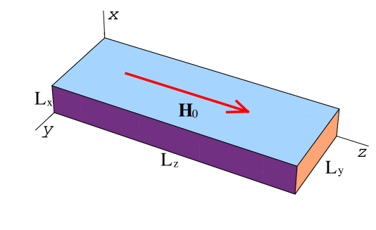
Figure 1: A schematic view of YIG film. The arrow indicates the direction of magnetic field ${\rm{\mathbf{H}}}_{0}$ applied to it.

As is known, in the case where the crystal has the ferromagnetic spin ordering (for definiteness, the direction of the $z$-axis is the axis of “easy” magnetization, which, thus, will be the quantization axis), each elementary excitation corresponds to one “inverted” spin in the site ${\rm{\bf l}}$.^35,36 (Strictly speaking, for an arbitrary spin $S$ of a paramagnetic ion, the number of such excitations (spin levels) on the site can reach $2S$, but for further calculations such an increase is not significant since we restrict ourselves to the so-called “onemagnon” approximation, i.e., we assume that there is no more than one excitation in the site). From linear combinations of these states using known rules it is easy to construct eigenstates of the multi-site translationally invariant system in a form of spin waves with amplitudes $\psi_{\rm{\bf q}}({\rm{\bf l}})$, a direct form of which depends on boundary conditions. For simplification (see Ref. 36) the periodic boundary conditions are usually used, when the amplitudes are

$$\psi_{\rm{\bf q}}({\rm{\bf l}})=\prod\limits_{j=x,y,z}{L_{j}}^{-\frac{1}{2}}e^{iq_{j}l_{j}},\quad q_{j}=\frac{2\pi k_{j}}{L_{j}},\quad k_{j}=0,1,...,L_{j}-1,$$ (2.1)

i.e., have a form of plane waves, in which the dimensionless vector ${\rm{\bf l}}$ enumerates the lattice sites: $l_{j}=1,{\kern 1.0pt}\,2,...,L_{j}$, and the dimensionless wave vector $q_{j}=\tilde{q}_{j}a_{j}$ runs through a discrete set with a step $\Delta q_{j}=2\pi/L_{j}$ within the first Brillouin zone ($0\leq q_{j}<2\pi)$. In the case of free spins on the boundary the solution of the problem with appropriate boundary conditions gives somewhat other values for the amplitudes, namely (cf. Eq. (2.1))

$$\psi_{\rm{\bf q}}({\rm{\bf l}})=\prod\limits_{j=x,y,z}{L}^{-\frac{1}{2}}_{j}\gamma(q_{j})\cos q_{j}(l_{j}-\tfrac{1}{2}),\quad q_{j}=\frac{\pi k_{j}}{L_{j}},$$ (2.2)

$$\quad k_{j}=0,1,...,L_{j}-1,\quad\gamma(0)=1,\quad\gamma(q\neq 0)=\sqrt{2}.$$

(It is interesting to note that the wave function has this form only in the case of magnons, and if we consider, for example, particles moving in a lattice with the conditions on the boundary fixed for amplitudes, then in this case $\psi_{\rm{\bf q}}({\rm{\bf l}})\sim\prod\limits_{j}{\sin q_{j}l_{j}}$). They, as is easy to verify (see the Appendix), define eigenfunctions of the arising problem on the eigenvalues of the Hamiltonian of the system and define the full set of standing waves. The Brillouin zone is defined somewhat differently: $0\leq q_{j}<\pi$, and the discrete step $\Delta q_{j}=\pi/L_{j}$.

Whatever the boundary conditions for spins, they have little effect on the spectrum of ferromagnons determined mainly by the strong exchange interaction $J$, which for simplicity is assumed to be isotropic. In this case, a kinetic component of the spectrum can be represented by expression valid for the case of both types of the boundary conditions

$$\varepsilon_{kin}({\rm{\bf q}})=4J\sum\limits_{j=x,y,z}{\sin^{2}\frac{q_{j}}{2}}.$$ (2.3)

In the long-wavelength region $q_{j}\ll\pi$ the spectrum, as follows from Eq. (2.3) takes the usual “quadratic” form:

$$\varepsilon_{kin}({\rm{\bf q}})=J{\rm{\bf q}}^{2},$$ (2.4)

and it is easy to write it through the length of edges ${\rm L}_{j}$, periods $a_{j}$ of the crystal lattice and the effective mass $m_{\scriptscriptstyle{M}}$ of magnons directly related to the exchange integral $J$.

The written expression (2.4) does not account for the gap, the value of which in ferromagnetic materials can be of a dual nature. Without a magnetic field it is determined by the magnetic anisotropy and is generally small. For the gap in the case of YIG, more important is an external magnetic field which is applied along the magnetization vector and provides a variation in a fairly wide range of the quantity $\varepsilon_{0}=\mu_{\scriptscriptstyle{B}}gH_{0}$ ($\mu_{\scriptscriptstyle{B}}$ is the Bohr magneton, and $g$ is the $g$-factor of three-valent iron ion close to two), taking into account which the magnon spectrum takes the final form

$$\varepsilon({\rm{\bf q}})=\varepsilon_{0}+\varepsilon_{kin}({\rm{\bf q}}).$$ (2.5)

The minimum values of the kinetic energy of magnons, following from Eqs. (2.4) and (2.5), are provided by the smallest wave vectors from the range enabled for them. In YIG films, as already mentioned, it is not the case, and in the direction of magnetization, or in our case, the quantization axis $z$, due to the contribution of the same anisotropic interactions the minimum is reached at some finite value of the $z$-projection of the wave vector ${\rm{\bf q}}$: $q_{z}=q_{0}$. An accurate albeit cumbersome expression for the magnon dispersion in YIG with taking into account its peculiar downward is known (see Ref. 32), but for the problem of BEC it is sufficient also to restrict to the quadratic approximation for the anisotropic component. Then the kinetic energy of magnons can be expressed as^4,20

$$\varepsilon_{kin}({\rm{\bf q}})=J\left[{{\rm{\bf q}}_{\bot}^{2}+\eta(q_{z})(q_{z}-q_{0})^{2}}\right].$$ (2.6)

In what follows, the dimensionless coefficient $\eta(q_{z})$ will be assumed to be equal to unity without loss of generality. Assuming an ideality of long-wavelength magnons (recall that their interaction with each other $\sim({\rm{\bf q}}_{1}{\rm{\bf q}}_{2})^{2}$ (Ref. 30), and, thus, is not large), we need to calculate the partition function $Z$ of the grand canonical ensemble, which has the form

$$\ln Z=-\sum\limits_{\rm{\bf q}}\ln\left\{1-{\mathrm{e}}^{[\mu-\varepsilon({\rm{\bf q}})]/T}\right\},$$ (2.7)

where $\varepsilon({\rm{\bf q}})$ is the magnon energy defined in Eq. (2.5), with the wave number ${\rm{\bf q}}=(q_{x},q_{y},q_{z})$, and $\mu$ is the chemical potential of magnons. In the expression (2.7) and below we use the system of units $\hbar=k_{B}=1$, restoring the dependence on the fundamental values only where it is necessary. Then for the average number of Bose-particles (the occupation number) in a quantum state with a given wave vector, we have

$$n_{\rm{\bf q}}=\frac{1}{{\mathrm{e}}^{[\varepsilon({\rm{\bf q}})-\mu]/T}-1}\,.$$ (2.8)

As follows from Eqs. (2.7) and (2.8), the range of the value of $\mu$ is limited by a minimum value of the energy. In the case of the dispersion law (2.5) in the presence of the gap we come to the inequality $\mu<\varepsilon_{0}$, where $\varepsilon_{0}=\varepsilon({\rm{\bf q}}_{0})$, and ${\rm{\bf q}}_{0}=(0,0,q_{0})$, and $\varepsilon_{0}$ is completely determined by an external static field. But if $\mu\to\varepsilon_{0}$, then $n_{{\rm{\bf q}}_{0}}\to\infty$ in a finite volume, which is not possible.

To avoid this contradiction, we note that the chemical potential as an independent thermodynamic variable is a convenient parameter in the theory, but quite formal quantity if an experiment is considered where $\mu$, as a rule, can be found only indirectly (for example, by calculating it from the measured average number of particles or from other observations). It is easy, however, to make sure that in studying the ideal Bose gas, the chemical potential can be completely eliminated from thermodynamic formulas, by replacing it with another independent variable that has a clear physical meaning. If it is a BEC, a quite justified and convenient quantity is the number of particles on the lowest level $n_{0}$. Indeed, using Eqs. (2.5) and (2.8), we introduce the thermodynamic variable

$$n_{0}=\frac{1}{{\mathrm{e}}^{(\varepsilon_{0}-\mu)/T}-1},$$ (2.9)

which makes it possible to find not only $\mu=\varepsilon_{0}-T\ln(1+n_{0}^{-1})$, but all the others (for ${\rm{\bf q}}\neq{\rm{\bf q}}_{0})$) occupation numbers

$$n_{{\rm{\bf q}}}=\frac{1}{(1+n_{0}^{-1}){\mathrm{e}}^{[\varepsilon({\rm{\bf q}})-\varepsilon_{0}]/T}-1}=\frac{n_{\rm{\bf q}}^{sat}n_{0}}{n_{{\rm{\bf q}}}^{sat}+n_{0}+1}\,.$$ (2.10)

In Eq. (2.10) we use the notation for the number

$$n_{\rm{\bf q}}^{sat}=\frac{1}{{\mathrm{e}}^{\varepsilon_{kin}({\rm{\bf q}})/T}-1}\,,$$ (2.11)

which is independent neither of the magnon spectrum gap in the magnon spectrum defined by an external magnetic field nor of their chemical potential and, as can be seen, which determines the maximum (saturating) capacity of the state relative to accumulation in it of Bose particles at a given temperature. The replacement, Eq. (2.9), allows to avoid the non-physical asymptotic $n_{0}\to\infty$ and to study the most interesting for BEC situation when $\mu\to\varepsilon_{0}$. The parameterization of unknown quantities by the number $n_{0}$ is convenient also because in fact the condensate is identified with it, or $N_{\scriptscriptstyle{BEC}}=n_{0}$, and in addition, there is a possibility to go correctly to the thermodynamic limit when it is necessary.

Taking the condition $n_{0}\gg n_{\rm{\bf q}}^{sat}$, corresponding to the condensation regime, from Eq. (2.10) for all ${\rm{\bf q}}\neq{\rm{\bf q}}_{0}$ we obtain the expansion

$$n_{\rm{\bf q}}=n_{\rm{\bf q}}^{sat}\left[1-\left(\frac{n_{\rm{\bf q}}^{sat}+1}{n_{0}}\right)+\left(\frac{n_{\rm{\bf q}}^{sat}+1}{n_{0}}\right)^{2}-...\right],$$ (2.12)

which indicates that the value Eq. (2.11) is indeed the maximum possible (for the formal condition $n_{0}\to\infty)$) occupation number of the ${\rm{\bf q}}$-state. The expansion (2.12) can also be used in writing other thermodynamic quantities. Thus, the average number of particles becomes

$$N=\sum\limits_{{\rm{\bf q}}}n_{\rm q}=n_{0}+\sum\limits_{{\rm{\bf q}}\neq{\rm{\bf q}}_{0}}n_{\rm q}=n_{0}+N_{exc},$$ (2.13)

where the quantity

$$N_{exc}=\sum\limits_{{\rm{\bf q}}\neq{\rm{\bf q}}_{0}}n_{\rm{\bf q}}^{sat}\left[1-\left(\frac{n_{\rm{\bf q}}^{sat}+1}{n_{0}}\right)+\left(\frac{n_{\rm{\bf q}}^{sat}+1}{n_{0}}\right)^{2}-...\right]\approx N_{sat}-\frac{\delta N_{sat}}{n_{0}}$$ (2.14)

for a given $n_{0}$ defines the total density of magnons in all excited states. From it in the last relation we separated out the number

$$N_{sat}=\sum\limits_{{\rm{\bf q}}\neq{\rm{\bf q}}_{0}}n_{\rm{\bf q}}^{sat},$$ (2.15)

which specifies the maximum, reached at the same (see above) condition $n_{0}\to\infty$, number of thermal excitations, and the coefficient

$$\delta N_{sat}=\sum\limits_{{\rm{\bf q}}\neq{\rm{\bf q}}_{0}}n_{\rm{\bf q}}^{sat}(n_{\rm{\bf q}}^{sat}+1)$$ (2.16)

for the first in $1/n_{0}$ correction determining thermal fluctuations of the quantity Eq. (2.15). In this case, it is seen that regardless of the specific type (type of Eq. (2.6)) of the dispersion of elementary excitations the both quantities $N_{sat}$ and $\delta N_{sat}$ are monotonically increasing functions of temperature, since with increasing $T$ all occupation numbers $n_{\rm{\bf q}}^{sat}$ are also growing.

Finally, combining Eqs. (2.13), (2.15), and (2.16) in the natural assumption $N\gg 1$ (and, of course, $n_{0}\gg 1)$), we arrive at the equation

$$N\simeq n_{0}+N_{sat}-\frac{\delta N_{sat}}{n_{0}}$$ (2.17)

for finding the density of a Bose condensate. In particular, from Eq. (2.17) it follows that the critical temperature of BEC is a solution of the equation $N_{sat}(T_{\scriptscriptstyle{BEC}})=N$ and already depends on both the total concentration of particles and the specific form of the spectrum. And an explicit expression for the temperature $T_{\scriptscriptstyle{BEC}}$ is also defined by the dimensionality and even the shape of a sample, including the conditions on all its boundaries.

Similar quantities can be introduced for thermal magnons when $\mu=0$, separating in the same way the equilibrium population

$$n_{0}^{th}=\frac{1}{{\mathrm{e}}^{\varepsilon_{0}/T}-1}$$ (2.18)

and representing, respectively,

$$n_{\rm{\bf q}}^{th}=\frac{n_{\rm{\bf q}}n_{0}^{th}}{n_{\rm{\bf q}}+n_{0}^{th}+1},$$ (2.19)

where $n_{\rm{\bf q}}$ is the same occupation number Eq. (2.12) as in Eq. (2.10). Remembering now that under pumping all the populations can be divided into two components: $n_{\rm{\bf q}}=n^{th}_{\rm{\bf q}}+n_{\rm{\bf q}}^{pump}$, with the help of Eqs. (2.14) and (2.19) we find that for all ${\rm{\bf q}}\neq{\rm{\bf q}}_{0}$

$$n_{\rm{\bf q}}^{pump}\approx\frac{\mu}{T}n_{\rm{\bf q}}(n_{\rm{\bf q}}+1).$$ (2.20)

In other words, because of the condition $\mu\ll T$, the populations of excited states are little changed, while the density of the pumped particles in a Bose condensate behaves completely different

$$n_{0}^{pump}\approx\frac{T}{\mu_{\scriptscriptstyle B}gH_{0}}\frac{\mu}{(\mu_{\scriptscriptstyle B}gH_{0}-\mu)},$$

or can be arbitrarily large when approaching $\mu\to\mu_{\scriptscriptstyle B}gH_{0}$. Moreover, from the last expression it follows that for the condensate state (in contrast to Eq. (2.20)), on the contrary, there is even an “enhancement factor” because $T\gg\mu_{\scriptscriptstyle B}gH_{0}$. To some extent, the increase due to the growth of the total number of excitations of the quantity $n_{0}$ only is consistent with the description of the magnon BEC based on the phenomenological approach, in which the dynamic macroscopic magnetization, which is identified with the condensate, is entirely caused by pumping¹⁰ (see also Ref. 4).

As a result we come to the conclusion mentioned already earlier: Magnons created in a thermally populated ferro-system by an intense electromagnetic pump are accumulates mainly on its lowest level. Consequently, such a subsystem of quasiparticles artificially created at any temperature, satisfying the inequality $T\gg\varepsilon_{0}$ (1.2), by itself formally (if the lifetime allows) undergoes BEC, coexisting with a powerful thermal collective of particles identical to it. It is this BEC which is essentially high-temperature, and its accompanying process is nothing like a turning of the magnetic crystal with the anomalously excited lowest mode into the magnon tuning fork.

3 A spatial distribution of density of excitations

We define the single-particle distribution function of magnons as follows:

$$\rho({\rm{\bf l}})=\sum\limits_{\rm{\bf q}}{n_{\rm{\bf q}}}\left|{\psi_{\rm{\bf q}}({\rm{\bf l}})}\right|^{2},$$ (3.1)

where $\psi_{\rm{\bf q}}({\rm{\bf l}})$ is the amplitude of a spin wave. In the case of periodic boundary conditions (2.1) $|\psi_{\rm{\bf q}}({\rm{\bf l}})|^{2}=(L_{x}L_{y}L_{z})^{-1}$ and the distribution function Eq. (3.1) does not depend on ${\rm{\bf l}}$. For free boundary conditions the amplitude is real and expressed in the form of a “standing wave”, Eq. (2.1). Therefore, separating in the sum Eq. (3.1) the term with the highest value of $n_{\rm{\bf q}}$, namely at ${\rm{\bf q}}={\rm{\bf q}}_{0}$, according to Eq. (2.6), we obtain

$$\rho({\rm{\bf l}})=\frac{2n_{0}}{L_{x}L_{y}L_{z}}\cos^{2}q_{0}(l_{z}-\tfrac{1}{2})+\sum\limits_{{\rm{\bf q}}\neq{\rm{\bf q}}_{0}}{n_{\rm{\bf q}}}{\psi^{2}_{\rm{\bf q}}({\rm{\bf l}})}.$$ (3.2)

With increasing $n_{0}$ the second term in Eq. (3.2) reaches the limit

$$\rho_{sat}({\rm{\bf l}})=\sum\limits_{{\rm{\bf q}}\neq{\rm{\bf q}}_{0}}{n^{sat}_{\rm{\bf q}}}{\psi^{2}_{\rm{\bf q}}({\rm{\bf l}})},$$

So, sooner or later, the first term in Eq. (3.2) becomes dominant. As a result, $\rho({\rm{\bf l}})$ oscillates with a frequency $q_{0}$ along the $z$-axis. Thus, qualitatively the mechanism of the appearance of the periodic structure in the spatial density of magnons turns out to be relatively simple. However, an exact calculation of the function Eq. (3.2) is rather cumbersome, so it makes sense to consider first the one-dimensional case. This will allow to understand how and under what conditions the lattice can be formed in the pumped system of magnons at temperatures exceeding the spectral gap.

3.1. A one-dimensional ferromagnet.

In the case of free boundary conditions the wave function and the quasi-momentum are written as follows (see the Appendix):

$$\psi_{q}(l)=L^{-\frac{1}{2}}\gamma(q)\cos q(l-\tfrac{1}{2}),\quad q=\frac{\pi k}{L},\quad k=0,1,...,L-1\,.$$ (3.3)

The distribution Eq. (3.1) is also easily rewritten and takes the form

$$\rho(l)=\sum\limits_{q}{n_{q}}{\psi^{2}_{q}(l)},$$ (3.4)

in which

$$n_{q}=\frac{n_{q}^{sat}n_{0}}{n_{q}^{sat}+n_{0}+1},\quad n_{q}^{sat}=\frac{1}{{\mathrm{e}}^{\varepsilon_{kin}(q)/T}-1}\,.$$ (3.5)

Consider first the “monotonous” dispersion $\varepsilon(q)=\varepsilon_{0}+Jq^{2}$. Because the quasi-momentum $q$ is a discrete quantity (see Eq. (3.3)), instead of the occupation number $n_{q}$ we introduce the function of an integer argument

$$f(k)=n_{q}=\frac{1}{e^{\delta+\omega^{2}k^{2}}-1}\,,\quad\delta=\ln(1+n_{0}^{-1}),\quad\omega^{2}=\frac{J}{\pi^{2}L^{2}T}.$$ (3.6)

Then the spatial density of magnons Eq. (3.4) for the case Eq. (2.10) can be written as the sum

$$\rho(z)=\frac{1}{L}\sum\limits_{k=0}^{\infty}{f(k)\gamma^{2}(k)\cos^{2}\pi kz=\frac{1}{2L}\left[{\rho_{1}(z)+\rho_{1}(0)}\right]},$$ (3.7)

where the variable $z=(l-1/2)/L$ varies in the range $0<z<1$. $\rho_{1}(z)$ denotes the sum

$$\rho_{1}(z)=\sum\limits_{k=-\infty}^{\infty}{f(k)\cos 2\pi kz}.$$ (3.8)

Note that from the definition Eq. (3.7) it follows that $\rho(z)=\rho(1-z)$, i.e., the magnon density is a symmetric function with respect to the point $z=1/2$.

Considering the variable $k$ as complex, we express the desired sum Eq. (3.8) via the contour integral

$$\rho_{1}(z)=\oint\limits_{C_{1}}\frac{{\rm d}k\,{\mathrm{e}}^{2\pi ikz}}{{\mathrm{e}}^{2\pi ik}-1}\,f(k)\,,$$ (3.9)

where the integration path $C_{1}$ is shown in Fig. 2.

Figure 2: $C_{1}$, $C_{2}$ – are the contours of integration in the integrals Eqs. (3.9) and (3.17). The crosses indicate the closest to the real axis of the complex $k$-plane poles of the functions $f(k)$, Eq. (3.6), and $F(k)$, Eq. (3.31).

Since, as is easily seen, the function Eq. (3.6) has simple poles at $k=k_{j}$, where

$$\omega k_{j}=\pm iu_{j}\pm\frac{\pi j}{u_{j}},\quad u_{j}=\sqrt{\frac{\delta}{2}+\sqrt{\frac{\delta^{2}}{4}+\pi^{2}j^{2}}},\quad j=0,1,...\quad,$$ (3.10)

the integral Eq. (3.9) is expressed by the sum of residues at these poles, in which only contributions from the poles closest to the real axis in the complex $k$-plane are taken into account. After having done the necessary calculations, we obtain the expression

$$\rho_{1}(z)={\frac{\pi^{2}}{\omega^{2}}}\frac{\cosh\alpha(1-2z)}{\alpha\cosh\alpha}+o[{\mathrm{e}}^{-\pi^{3/2}z/\omega}],\quad\alpha=\frac{\pi}{\omega}\sqrt{\delta}\,,$$ (3.11)

included in the formula Eq. (3.7) for $\rho(z)$. It, however, contains the quantity $\rho_{1}(0)$, which does not follow from Eq. (3.11) because of the large value of corrections to $z=0$. To calculate $\rho_{1}(z)$ in the range of small values of $z$ it is necessary to replace Eq. (3.9) with the representation

$$\rho_{1}(z)=-\frac{i}{2}\oint\limits_{C_{1}}{\rm d}k\,f(k)\cos 2\pi kz\,\cot\pi k=$$

$$=\frac{2\pi^{2}}{\omega^{2}\alpha}\frac{\cosh 2\alpha z}{{\mathrm{e}}^{2\alpha}-1}+\int\limits_{0}^{\infty}{\rm d}k\,f(k)\cos 2\pi kz+o[{\mathrm{e}}^{-\pi^{3/2}/\omega}],$$ (3.12)

from where we find

$$\rho_{1}(0)=\frac{2\pi^{2}}{\omega^{2}\alpha({\mathrm{e}}^{2\alpha}-1)}+\frac{\sqrt{\pi}}{2\omega}Li_{\frac{1}{2}}(e^{-\delta})=n_{0}\alpha\cosh\alpha+\frac{\sqrt{\pi}}{\omega}\left[{Li_{\frac{1}{2}}(e^{-\delta})-\sqrt{\frac{\pi}{\delta}}}\right],$$ (3.13)

where $Li_{\frac{1}{2}}(e^{-\delta})$ – is the polylogarithm.³⁷ The found dependencies solve the problem of the spatial distribution of magnons, but in the assumption of a quadratic spectrum it is smooth not only for the case of periodic boundary conditions, but also in the case of free boundaries.

The situation is different if the spectrum has a minimum at ${q}={q}_{0}\neq 0$, which in the one-dimensional case can be represented without loss of generality as

$$\varepsilon(q)=\varepsilon_{0}+J(q-q_{0})^{2}.$$ (3.14)

Then, using Eq. (3.14), the expression (3.4) takes the form

$$\rho(z)=\frac{1}{L}\sum\limits_{k=0}^{\infty}f(k-k_{0})\gamma^{2}(k)\cos^{2}\pi kz=\frac{1}{L}[A_{latt}(z)\cos^{2}\pi k_{0}z+A(z)],$$

$$A_{latt}(z)=2\rho_{1}(z),\quad A(z)=\rho_{1}(0)-\rho_{1}(z)-\rho_{2}(0)-\rho_{2}(z)-f(k_{0}),$$ (3.15)

in which we separated out the term oscillating with a characteristic period $\sim k_{0}^{-1}=\pi/(Lq_{0})$ completely caused by the presence of cosine in the wave function Eq. (3.3). The function $\rho_{1}(z)$ in Eq. (3.15) is defined in Eq. (3.8), and the function

$$\rho_{2}(z)=\sum\limits_{k=1}^{\infty}{f(k+k_{0})\cos 2\pi kz}$$ (3.16)

can also be represented by the contour integral

$$\rho_{2}(z)=\oint\limits_{C_{2}}\frac{{\rm d}k\,{\mathrm{e}}^{2\pi ikz}}{{\mathrm{e}}^{2\pi ik}-1}\,f(k+k_{0})\,,$$ (3.17)

where the contour of integration $C_{2}$ is shown in Fig. 2. A direct calculation of this integral as well as Eq. (3.9) we perform in two steps. First, we assume that the aboveintroduced parameters $\delta$ and $\omega$ are small, and the value of $k_{0}$ is high that corresponds to the situation which occurs in study of YIG. Then, using the exact value of the integral

$$\int\limits_{-\infty}^{\infty}{\frac{{\rm d}\xi\,{\mathrm{e}}^{2\pi\xi z}}{{\mathrm{e}}^{2\pi\xi}+1}}=\frac{1}{2\sin\pi z}$$

and expanding in a series the function $f(k+k_{0})$ in the neighborhood of the point $k=1/2$, we find the asymptotic expansion of the integral Eq. (3.17). In the first order we have

$$\rho_{2}(z)\simeq-f_{0}\,{\rm Re}\left(\frac{{\mathrm{e}}^{-\kappa}}{1-{\mathrm{e}}^{-2\kappa-2\pi iz}}\right),$$ (3.18)

where $f_{0}=f(k_{0}+1/2)$, $\kappa=f_{1}/2f_{0}$ and $f_{1}=f^{\prime}(k_{0}+1/2)$. The expression (3.18) is a good approximation in the range of $k_{0}^{-1}<z<1-k_{0}^{-1}$, and at lower values of $z$ it is necessary to use the representation

$$\rho_{2}(z)=-\frac{i}{2}\oint\limits_{C_{2}}{\rm d}k\,f(k+k_{0})\cos 2\pi kz\,\cot\pi k=I_{1}(z)+I_{2}(z),$$ (3.19)

$$I_{1}(z)=2{\rm Re}\int\limits_{C_{-}}\frac{{\rm d}k\,\cos 2\pi kz}{{\mathrm{e}}^{2\pi ik}-1}\,f(k+k_{0}),\quad I_{2}(z)=\int\limits_{1/2}^{\infty}{\rm d}k\,f(k+k_{0})\cos 2\pi kz,$$

in which $C_{-}$ denotes a part of the contour $C_{2}$, which lies in the lower half-plane of the complex variable $k$. An approximate expression for the first integral Eq. (3.19) can be obtained by analogy with Eq. (3.18) which gives

$$I_{1}(z)\simeq-\frac{1}{24}(2\pi zf_{0}\sin\pi z-f_{1}\cos\pi z).$$ (3.20)

The second integral can also be found after simple calculations. We write it only for the point $z=0$

$$I_{2}(0)=\frac{1}{\omega\sqrt{\delta}}\,\arctan\left[\frac{\sqrt{\delta}}{\omega(k_{0}+1/2)}\right]+\frac{\sqrt{\pi}}{2\omega}Li_{\frac{1}{2}}(e^{-\delta})-\frac{\pi}{2\omega\sqrt{\delta}}+$$

$$+\int\limits_{0}^{k_{0}+1/2}{\rm d}k{\left({\frac{1}{\delta+\omega^{2}k^{2}}-\frac{1}{{\mathrm{e}}^{\delta+\omega^{2}k^{2}}-1}}\right)}\,.$$ (3.21)

As a result, from Eqs. (3.18)–(3.21) it is seen that even at a small distance from the edges of the chain between the two contributions $\rho_{2}(z)$ and $\rho_{2}(0)$ there is the inequality $\rho_{2}(0)\gg\rho_{2}(z)$, and only in the immediate vicinity of the boundaries, these contributions become comparable. Then for the amplitude Eq. (3.15) of the periodic structure using Eq. (3.11) we find

$$A_{latt}(z)=2n_{0}\alpha\,\coth\alpha-\frac{4\pi^{2}}{\omega^{2}}\lambda(z),\quad\lambda(z)=\frac{\sinh(\alpha z)\,{\kern 1.0pt}\sinh\alpha(1-z)}{\alpha\sinh\alpha}.$$ (3.22)

The expression for the non-uniform and not-lattice distribution $A(z)$ in Eq. (3.15) has a more complicated form, but after calculating the integrals Eqs. (3.17) and (3.19) with Eqs. (3.20) and (3.21) one can obtain fairly simple approximate formula for it

$$A(z)=\frac{2}{\omega^{2}}\left[{\pi^{2}\lambda(z)-O\left({\frac{1}{2k_{0}+1}}\right)}\right].$$ (3.23)

Using the explicit form of the functions $A_{latt}(z)$ and $A(z)$, which enters the distribution of the magnon density in the chain Eq. (3.15), one can find the conditions for the formation of the magnon lattice. The corresponding periodic structure arises in the case when its amplitude $A_{latt}(z)$ exceeds the value of the relatively smooth contribution $A(z)$, which is physically controlled by the ratio $a_{latt}(z)=A_{latt}(z)/A(z)$. For small $n_{0}$ of the condensate component of Bose particles, or if the inequalities $\omega^{2}n_{0}\ll 1$, $\alpha\gg 1$ are satisfied, the coefficient $a_{latt}(z)\approx\tfrac{1}{2}{\mathrm{e}}^{-2\alpha z}\ll 1$, so that the oscillations cannot appear as, in fact, expected. Moreover, there is no periodic structure in equilibrium, although the population $n_{0}^{th}$ (see Eq. (2.18)) is the greatest. On the contrary, in the case of large numbers $n_{0}$ and the small gap in the magnon spectrum when $\alpha\ll 1$, the quantity $a_{latt}(z)\approx n_{0}\omega^{2}/[\pi^{2}z(1-z)]\gg 1$, and the lattice of the excitation density dominates over the background. In this case, the critical (transition) density of a Bose condensate, as is easily seen, is its value at which $a_{latt}(z)\approx 1$, or $n_{0}\approx 1/\omega^{2}=\pi^{2}L^{2}T/J$. It should also be noted that the appearance of the modulated structure at a relatively smooth background of the density distribution of pumped excitations takes place with increasing the pumping (i.e., the density of the Bose condensate) gradually, not abruptly, as stated in Ref. 9, and does not require the assumption about the presence in the system of two condensates²⁵ or an abnormally strong damping of quasiparticles (magnons).

3.2. A three-dimensional ferromagnet.

We represent the ratio $\varepsilon_{kin}({\mathbf{q}})/T$ in terms of dimensionless parameters

$$\frac{\varepsilon_{kin}({\mathbf{q}})}{T}=\omega_{x}^{2}k_{x}^{2}+\omega_{y}^{2}k_{y}^{2}+\omega_{z}^{2}(k_{z}-k_{0})^{2},$$ (3.24)

where $k_{0}=22282$ is the integer number closest to $\tilde{q}_{0}{\rm L}_{z}/\pi$ at ${\rm L}_{z}=2$ cm, and

$$\omega_{x}=\frac{{\rm L}_{z}}{{\rm L}_{x}}\omega,\quad\omega_{y}=\frac{{\rm L}_{z}}{{\rm L}_{y}}\omega,\quad\omega_{z}=\omega=\frac{\pi}{{\rm L}_{z}}\sqrt{\frac{J}{T}}.$$ (3.25)

If the constant $J$ is expressed via the magnon mass $m_{mag}$ (in YIG it is ${}\simeq 5m_{e}$), we obtain, that in the room-temperature range ($T\simeq 300\,K$)

$$\omega=\frac{\pi\hbar}{{\rm L}_{z}}(2m_{mag}k_{\scriptscriptstyle B}T)^{-\frac{1}{2}}\simeq 8.53\times 10^{-8}.$$ (3.26)

For a quantitative description of the effect of oscillations it is necessary to calculate the sum in rhs of Eq. (3.2). But instead it is easier to consider the magnon density averaged over the coordinates ${\mathbf{l}}_{\perp}$, namely

$$\bar{\rho}(z)=L_{z}\sum_{{\mathbf{l}}_{\perp}}\rho({\mathbf{l}})=\sum_{{\mathbf{q}}}n_{{\mathbf{q}}}\gamma^{2}(q_{z})\cos^{2}q_{z}(l_{z}-\tfrac{1}{2})=\sum_{k_{z}=0}^{\infty}F(k_{z}-k_{0})\gamma^{2}(k_{z})\cos^{2}\pi k_{z}z,$$ (3.27)

where

$$F(k_{z}-k_{0})=\sum_{{\mathbf{q}}_{\perp}}n_{{\mathbf{q}}},\quad z=\frac{l_{z}-1/2}{L_{z}}.$$ (3.28)

Represent $\bar{\rho}(z)$, similar to the one-dimensional case Eq. (3.15), as:

$$\bar{\rho}(z)=A_{latt}(z)\cos^{2}\pi k_{0}z+A(z),$$ (3.29)

$$A_{latt}(z)=2\rho_{1}(z),\quad A(z)=\rho_{1}(0)-\rho_{1}(z)-\rho_{2}(0)-\rho_{2}(z)-F(k_{0}),$$

where

$$\rho_{1}(z)=\sum_{k_{z}=-\infty}^{\infty}F(k_{z})\cos 2\pi k_{z}z,\quad\rho_{2}(z)=\sum_{k_{z}=1}^{\infty}F(k_{z}+k_{0})\cos 2\pi k_{z}z.$$ (3.30)

As can be seen from the definition Eq. (3.28), the function $F(k_{z})$ is a sum of Bose -terms of the type of Eq. (3.6)

$$F(k_{z})=\sum_{k_{x}=0}^{\infty}\sum_{k_{y}=0}^{\infty}\frac{1}{{\mathrm{e}}^{w}-1},$$ (3.31)

where

$$w=w(k_{x},k_{y},k_{z})=\delta+\omega_{x}^{2}k_{x}^{2}+\omega_{y}^{2}k_{y}^{2}+\omega_{z}^{2}k_{z}^{2}.$$ (3.32)

Therefore, to calculate $\rho_{1}(z)$ one can use the transformations Eq. (3.9) when $k_{0}^{-1}<z<1-k_{0}^{-1}$, of Eq. (3.12) when $0\leqslant z<k_{0}^{-1}$. As a result, we obtain for $\rho_{1}(z)$ a series representation

$$\rho_{1}(z)=\frac{\pi^{2}}{\omega_{z}^{2}}\sum_{k_{x}=0}^{\infty}\sum_{k_{y}=0}^{\infty}\frac{\coth\alpha_{z}(1-2z)}{\alpha_{z}\sinh\alpha_{z}},$$ (3.33)

where $\alpha_{j}$ denote the functions

$$\alpha_{x}=\alpha_{x}(k_{y},k_{z})=\frac{\pi}{\omega_{x}}\sqrt{\delta+\omega_{y}^{2}k_{y}^{2}+\omega_{z}^{2}k_{z}^{2}},$$

$$\alpha_{y}=\alpha_{y}(k_{x},k_{z})=\frac{\pi}{\omega_{y}}\sqrt{\delta+\omega_{x}^{2}k_{x}^{2}+\omega_{z}^{2}k_{z}^{2}},$$ (3.34)

$$\alpha_{z}=\alpha_{z}(k_{x},k_{y})=\frac{\pi}{\omega_{z}}\sqrt{\delta+\omega_{x}^{2}k_{x}^{2}+\omega_{y}^{2}k_{y}^{2}}.$$

When $\delta\ll 1$ and taking into account the smallness of the ratio $\omega_{z}/\omega_{x}$, $\omega_{z}/\omega_{y}$, for Eq. (3.33) there is a valid approximate expression

$$\rho_{1}(z)=\frac{\pi^{2}}{\omega_{z}^{2}}\,\frac{\coth\alpha(1-2z)}{\alpha\sinh\alpha}-\frac{\pi}{\omega_{z}\omega_{y}}\ln(1-{\mathrm{e}}^{-2\pi z\omega_{y}/\omega_{z}})=$$

$$=\frac{\alpha\coth\alpha}{\delta}+\frac{2\pi^{2}}{\omega_{z}^{2}}\,\frac{\sinh\alpha z\cdot\sinh\alpha(1-z)}{\alpha\sinh\alpha}-\frac{\pi}{\omega_{z}\omega_{y}}\ln(1-{\mathrm{e}}^{-2\pi z\omega_{y}/\omega_{z}}),$$ (3.35)

where $\lambda(z)$ is defined in Eq. (3.22) and $\alpha=\alpha_{z}(0,0)={\pi}\sqrt{\delta}/{\omega_{z}}$. The discarded contributions in Eq. (3.35) does not exceed the value ${\pi}{\mathrm{e}}^{-2\pi z\omega_{x}/\omega_{z}}/(2\omega_{x}\omega_{z})$. As before, for finding the value of $\rho_{1}(0)$ we use the transformation Eq. (3.12). Then

$$\rho_{1}(0)=\sum_{k_{z}=-\infty}^{\infty}F(k_{z})=R+I,$$ (3.36)

where $R$ is the sum of residues in the closest to the real axis poles of the function $F(k_{z})$

$$R=\frac{2\pi^{2}}{\omega_{z}^{2}}\sum_{k_{x}=0}^{\infty}\sum_{k_{y}=0}^{\infty}\frac{1}{\alpha_{z}({\mathrm{e}}^{2\alpha_{z}}-1)}\,.$$ (3.37)

Similarly to Eq. (3.35) we get for $R$ the approximate expression

$$R=\frac{2\pi^{2}}{\omega_{z}^{2}}\,\frac{1}{\alpha({\mathrm{e}}^{2\alpha}-1)}=\frac{\alpha\coth\alpha}{\delta}-\frac{\pi}{\omega_{z}}\,\frac{1}{\delta^{1/2}}\,,$$ (3.38)

and the neglected terms do not exceed ${\pi}{\mathrm{e}}^{-2\pi\omega_{y}/\omega_{z}}/({\omega_{y}\omega_{z}})$. $I$ on rhs of Eq. (3.36) denotes the integral

$$I=2\int\limits_{0}^{\infty}{\rm d}k_{z}\,F(k_{z}).$$ (3.39)

We apply consistently the transformation Eq. (3.7) to the summations in Eq. (3.31). Then, in particular, for the sum over $k_{y}$ we obtain

$$\sum_{k_{y}=0}^{\infty}\frac{1}{{\mathrm{e}}^{w}-1}=\frac{\pi^{2}}{\omega_{y}^{2}}\,\frac{1}{\alpha_{y}}\,\frac{1}{{\mathrm{e}}^{2\alpha_{y}}-1}+\frac{1}{2}\int\limits_{-\infty}^{\infty}\frac{{\rm d}k_{y}[1+\delta(k_{y})]}{{\mathrm{e}}^{w}-1}\,,$$ (3.40)

where $\delta(k)$ is the $\delta$-function of Dirac. Performing similarly to Eq. (3.40) the summation over $k_{x}$, we obtain for $F(k_{z})$ the following expression:

$$F(k_{z})=\frac{1}{4}\int\limits_{-\infty}^{\infty}\frac{{\rm d}k_{x}\,{\rm d}k_{y}}{{\mathrm{e}}^{w}-1}[1+\delta(k_{x})][1+\delta(k_{y})]+\frac{\pi^{2}}{2\omega_{x}^{2}}\int\limits_{-\infty}^{\infty}\frac{{\rm d}k_{y}}{\alpha_{x}}\,\frac{1+\delta(k_{y})}{{\mathrm{e}}^{2\alpha_{x}}-1}+\frac{\pi^{2}}{\omega_{y}^{2}}\sum_{k_{x}=0}^{\infty}\frac{1}{\alpha_{y}}\,\frac{1}{{\mathrm{e}}^{2\alpha_{y}}-1}.$$ (3.41)

Note that in the sum on rhs of Eq. (3.41) only the term with $k_{x}=0$ can remain, since the other terms are exponentially small: $\sim{\mathrm{e}}^{-2\pi\omega_{x}/\omega_{z}}$. Substituting Eq. (3.41) into Eq. (3.39) and integrating, we obtain for the integral $I$ the following expression:

$$I = \frac{\pi^{3/2}}{8\omega_{x}\omega_{y}\omega_{z}}Li_{\frac{3}{2}}({\mathrm{e}}^{-\delta})-\frac{\pi(\omega_{y}+\omega_{x})}{8\omega_{x}\omega_{y}\omega_{z}}\ln(1-{\mathrm{e}}^{-\delta})+\frac{\sqrt{\pi}}{8\omega_{z}}Li_{\frac{1}{2}}({\mathrm{e}}^{-\delta})-$$ (3.42)

$$-\frac{\pi}{4\omega_{y}\omega_{z}}\ln(1-{\mathrm{e}}^{-2\pi\delta^{1/2}/\omega_{x}})+\frac{\pi}{\omega_{y}\omega_{z}}G\biggl{(}\frac{2\pi}{\omega_{y}}\delta^{1/2}\biggr{)}+\frac{\pi}{2\omega_{x}\omega_{z}}G\biggl{(}\frac{2\pi}{\omega_{x}}\delta^{1/2}\biggr{)}\,,$$

where $G(t)$ denotes the integral

$$G(t)=\int\limits_{0}^{\infty}\frac{{\rm d}x}{\sqrt{t^{2}+x^{2}}}\,\frac{1}{{\mathrm{e}}^{\sqrt{t^{2}+x^{2}}}-1}\,.$$ (3.43)

The asymptotic expansion of $G(t)$ for $t\ll 1$ is of the form

$$G(t)=\frac{\pi}{2t}+\frac{1}{2}\ln\frac{t}{4\pi}+{\mathbb{C}}-\frac{\zeta(3)}{16\pi^{2}}t^{2}+O(t^{4}),$$ (3.44)

where ${\mathbb{C}}$ is the Euler s constant, $\zeta(\theta)$ is the $\zeta$-function of Riemann. The calculation of $\rho_{2}(z)$ is not fundamentally different from the one-dimensional case, Eq. (3.18). It is only necessary to replace the function $f(k)$, Eq. (3.6), with $F(k)$, Eq. (3.41). Then, for $k_{0}^{-1}<z<1-k_{0}^{-1}$ we obtain

$$\rho_{2}(z)=-F_{0}\,{\rm Re}\biggl{(}\frac{{\mathrm{e}}^{-\kappa}}{1-{\mathrm{e}}^{-2\kappa-2\pi iz}}\biggr{)}\,,$$ (3.45)

where $F_{0}=F(k_{0}+\tfrac{1}{2})$, $F_{1}=F^{\prime}(k_{0}+\tfrac{1}{2})$, $\kappa=\frac{F_{1}}{2F_{0}}$, and with $z=0$

$$\rho_{2}(0)=\tfrac{1}{2}I-I_{1}+I_{2},$$

$$I_{1}=\int\limits_{0}^{k_{0}+1/2}{\rm d}k_{z}\,F(k_{z}),\quad I_{2}={\rm Re}\int\limits_{C_{-}}\frac{{\rm d}k_{z}\,F(k_{z}+k_{0})}{{\mathrm{e}}^{2\pi ik_{z}}-1}.$$ (3.46)

Substituting into Eqs. (3.29) the relations (3.35), (3.36), (3.38), (3.45), and (3.46), we obtain an expression for $A(z)$. It looks quite lengthy, although it consists of elementary functions and simple integrals, numerical calculation of which is easy. It appears, however, that in the range $k_{0}^{-1}<z<1-k_{0}^{-1}$ a good approximation for the coefficients $A_{latt}(z)$, $A(z)$ is

$$A_{latt}(z)=2n_{0}\alpha\coth\alpha-\frac{4\pi^{2}}{\omega^{2}}\lambda(z),\quad A(z)=N_{sat}-\frac{\delta N_{sat}}{n_{0}}+\frac{2\pi^{2}}{\omega^{2}}\lambda(z),$$ (3.47)

where $\alpha={\pi}/(\omega_{z}\sqrt{n_{0}})$,

$$N_{sat}=\Omega\biggl{\{}\zeta\biggl{(}\frac{3}{2}\biggr{)}+\frac{4}{\sqrt{\pi}}\biggl{[}\varkappa\ln(1-\varkappa)+\omega_{x}\ln\biggl{(}\frac{\omega_{x}}{8\pi\omega_{y}^{2}}\biggr{)}\biggr{]}\biggr{\}}\,,\quad\delta N_{sat}=\frac{\pi\zeta(3)}{2\omega_{y}^{3}\omega_{z}},$$

$$\Omega=\frac{\pi}{8\,\omega_{x}\omega_{y}\omega_{z}}=L_{x}L_{y}L_{z}\biggl{(}\frac{m_{mag}k_{B}T}{2\pi\hbar^{2}}\biggr{)}^{3/2},\quad\varkappa=\omega_{z}(k_{0}+\tfrac{1}{2}).$$ (3.48)

A relative error of the approximate expression (3.47) in comparison with the exact one, Eq. (3.29), when $n_{0}>\omega_{y}^{-2}\gg\omega_{x}^{-2}$, does not exceed $0.5\times 10^{-3}$. As can be seen from Eq. (3.47), the amplitude of oscillations $A_{latt}(z)$ decreases with distance along the coordinate $z$ from boundaries of the film and the background contribution, by contrast, increases due to the terms proportional to the function $\lambda(z)$, Eq. (3.22). The graph of this function for some $n_{0}$ is shown in Fig. 3.

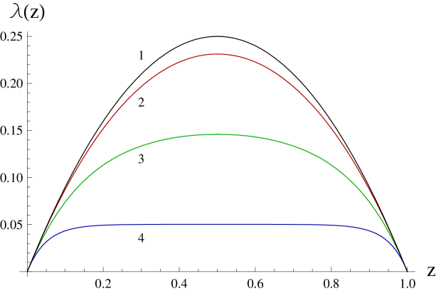
Figure 3: A behavior of the function $\lambda(z)$ for different $n_{0}$. The curves 2– 4 ($j>1$) correspond to $n_{0}=10^{3-j}\omega_{z}^{2}$, and the curve 1 is for $n_{0}=\infty$.

Note that the expression (3.47) for $A_{latt}(z)$ in the three-dimensional case is no different from the one-dimensional case, Eq. (3.22). However, the background contribution $A(z)$ is much higher than that of the one-dimensional problem, Eq. (3.23), so it is much easier to observe periodic spatial oscillations of $\rho(z)$ in thin films, and the thinner the better. Otherwise, an extremely large pumping is required, which would bring the value $n_{0}$ to values comparable with $N_{sat}$. It is this dependence on the pumping level which was observed in Ref. 38.

4 Conclusion

Although the conditions for the formation and observation of the magnon lattice in magnetic films such as YIG are hard enough, especially at room temperatures, there are a number of factors that contribute to this effect. In addition to the decrease of the film thickness noted above, this decrease of the temperature as well as, what is less obvious, the increase of the selectivity of the measuring apparatus, which suppresses frequencies outside the resonance region, to which in this case the frequency $\nu_{0}=\varepsilon_{0}/\hbar$ belongs. In YIG it is equal to $\simeq$2 GHz. In fact, we assume that the frequency response function of the receiver is characterized by

$$\Phi(u_{{\mathbf{q}}})=\frac{1}{1+Q^{2}(u_{{\mathbf{q}}}-u_{{\mathbf{q}}}^{-1})^{2}}\,,$$ (4.1)

where is the $Q$-factor, $u_{{\mathbf{q}}}=\varepsilon({\mathbf{q}})/\varepsilon_{0}$. Then, instead of $N_{sat}$ Eq. (3.48) there will be observed the other quantity $N_{obs}$

$$N_{obs}=\sum_{{\mathbf{q}}\neq{\mathbf{q}}_{0}}n^{sat}_{{\mathbf{q}}}\Phi(u_{{\mathbf{q}}}).$$ (4.2)

After calculations similar to those made in the calculation of Eq. (3.47), one can obtain the following approximate expression:

$$N_{obs}=\Omega\sqrt{\frac{\varepsilon_{0}}{\pi QT}}\biggl{[}\pi+\arctan(1+2v)-\arctan(1-2v)+\frac{1}{2}\ln\frac{1+2v+2v^{2}}{1-2v+2v^{2}}+v\ln(1+v^{-4}/4)\biggr{]},$$ (4.3)

where $v=\varkappa\sqrt{QT/\varepsilon_{0}}$. As can be seen from a comparison of Eqs. (3.48) and (4.3), the suppression of the background is determined by $\sqrt{\varepsilon_{0}/(QT)}$. For example, if $Q=20$ the numerical values of $N_{sat}$ and $N_{obs}$ are

$$N_{sat}\simeq 7.42\times 10^{16},\quad N_{obs}\simeq 3.68\times 10^{14},\quad N_{sat}/N_{obs}\simeq 200.$$

The poles in the complex k-plane of the function Eq. (4.1) are located far away from the real axis than the poles of the function $F(k)$, Eq. (3.28). Therefore the introduction of the function $\Phi(u_{q})$ does not affect the value of the coefficient $A_{latt}(z)$, Eq. (3.47). As a result, when $n_{0}\sim N_{obs}$ the expression for the magnon density is of very simple form

$$\bar{\rho}(z) = \biggl{[}2n_{0}\alpha\coth\alpha-\frac{4\pi^{2}}{\omega^{2}}\lambda(z)\biggr{]}\cos^{2}\pi k_{0}z+N_{obs}-\frac{\delta N_{sat}}{n_{0}}+\frac{2\pi^{2}}{\omega^{2}}\lambda(z)$$ (4.4)

$$\simeq 2n_{0}\cos^{2}q_{0}l_{z}+N_{obs}\,.$$

Fig. 4 shows graphs of the spatial density of magnons, calculated according to Eqs. (4.3) and (4.4). It is seen that the amplitude of oscillations increases on increasing the pumping and decreasing the distance from the edge of the sample along the axis $z$.

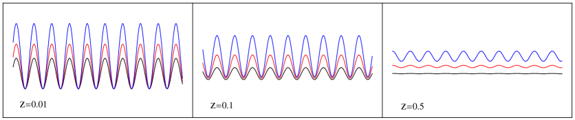
Figure 4: Oscillation of the spatial density of magnons for different parts of the film,    $z=(0.01,\,0.1,\,0.5)$, as a function of the $n_{0}=(0.5,\,1,\,2)\times 10^{14}\gg n_{0}^{th}$.

Note that the experiments²⁰ can provide the most accurate way to determine the position of a minimum in the dispersion. The last formula implies that for pumps that provide the value of $n_{0}$, which is at least two orders of magnitude smaller than $N_{sat}$, in a thin ferromagnetic film one can observe a standing spatial distribution of the density of the pumped magnons condensed due to relaxation in the lowest state with a period proportional to $q_{0}^{-1}$. Such a wave shows up as a lined (stripe) structure of the magnon density on the axis along which there is a dip in their dispersion laws $\varepsilon({\rm{\bf q}})$. A period of the structure is of $\pi/\tilde{q}_{0}$ and in the case of YIG is $\approx 0.92\ \mu$m, which does not depend on the size of the sample, as confirmed by measurements.³⁸ At the same time, as noted in the same paper,³⁸ the depth of the dips in the formed standing wave of the spatial distribution of the condensate depends strongly on the intensity of the pump $I_{pump}$, although it can be shown (see Ref. 21) that the contrast of the magnon lattice should not depend on the ratio $I_{pump}/(k_{\scriptscriptstyle B}T)$. Regarding the observations in Ref. 38 of edge dislocations in this lattice, their appearance by pairs corresponds to the conservation of the topological charge, but the mechanism of creation of these topological defects requires special consideration due to the fact that the presence of dislocations in the structure increases its energy, and hence the periodic condensate with the extended defects is an excited condensate. In addition, using magnon lattices one can scatter a light and explore other optical phenomena in which such a lattice may manifests itself.

We acknowledge S. G. Odulov for the discussion of optical lattices. The work was performed under the program of fundamental research of the Department of Physics and Astronomy, National Academy of Sciences of Ukraine.

Appendix

As is known, the projections of the spin operator ${\rm{\bf S}}=(S^{x},S^{y},S^{z})$ satisfy the commutation relations³⁵

$$\left[{S^{+},S^{-}}\right]=2S^{z},\quad\left[{S^{z},S^{\pm}}\right]=\pm S^{+},\quad S^{\pm}=S^{x}\pm iS^{y}.$$

We denote by $\chi_{S}$ eigenvector of the operator $S^{z}$ normalized per unit with the maximum eigenvalue $S$, so that

$$S^{z}\chi_{S}=S\chi_{S},\quad S^{+}\chi_{S}=0,\quad S^{-}\chi_{S}=\sqrt{2S}\chi_{S-1},\quad(\chi_{S},\chi_{S})=1.$$

The vector $\chi_{S-1}$ in Eq. (A.2) is also an eigenvector for the operator $S^{z}$ and for it the obvious relations follow from Eq. (A.1)

$$S^{z}\chi_{S-1}=(S-1)\chi_{S-1},\quad(\chi_{S-1},\chi_{S-1})=1,\quad(\chi_{S-1},\chi_{S})=0.$$

Let $\left|0\right\rangle$ is a ground (vacuum) state of the chain of $L$ spins, oriented along the direction $z$ and with a maximum value of the $z$-projection, and $\left|l\right\rangle$ is its single-particle excited state when the $z$-projection of the spin, which is located in the site $l$, is one less

$$\left|0\right\rangle=\prod\limits_{j=1}^{L}{\chi_{S}(j)},\quad\left|l\right\rangle=\prod\limits_{j=1}^{.l-1}{\chi_{S}(j){\kern 1.0pt}}\chi_{S-1}(l)\prod\limits_{j=l+1}^{L}{\chi_{S}(j)},$$

$$\langle 0|0\rangle=1,\quad\left\langle{0\left|l\right.}\right\rangle=0,\quad\left\langle{l\left|{l^{\prime}}\right.}\right\rangle=\delta_{l,l^{\prime}}.$$

If in the spin chain only nearest neighbors interact, its simplest Hamiltonian can be written in the form $\mathcal{H}=JH$, where

$$H=S^{-1}\sum\limits_{l=1}^{L-1}{(S^{2}-{\rm{\bf S}}_{l}{\rm{\bf S}}_{l-1})},\quad\left[{{\rm{\bf S}}_{l_{1}},{\rm{\bf S}}_{l_{2}}}\right]=0.$$

With the help of Eq. (A.1) is easy to find that $H\left|0\right\rangle=0$; for all $l$, satisfying the condition $1<l<L$,

$$H\left|l\right\rangle=2\left|l\right\rangle-\left|{l+1}\right\rangle-\left|{l-1}\right\rangle,$$

but on the states corresponding to the outermost sites this Hamiltonian acts differently

$$H\left|1\right\rangle=\left|1\right\rangle-\left|2\right\rangle,\quad H\left|L\right\rangle=\left|L\right\rangle-\left|{L-1}\right\rangle.$$

Let us introduce a linear combination of single-particle states

$$\left|q\right\rangle=\sum\limits_{l=1}^{L}{\psi_{q}(l)}\left|l\right\rangle$$

and act on it by the operator $H$ with taking into account Eq. (A.5)

$$H\left|q\right\rangle=\sum\limits_{l=1}^{L}{\left[{2\psi_{q}(l)-\psi_{q}(l-1)-\psi_{q}(l+1)}\right]}\left|l\right\rangle,$$

and the wave functions (amplitude) satisfy the free boundary conditions

$$\psi_{q}(0)=\psi_{q}(1),\quad\psi_{q}(L+1)=\psi_{q}(L).$$

From Eq. (A.6) it is seen that the bra-vector $\left|q\right\rangle$ is a onemagnon eigenstate of the spin Hamiltonian

$$H|q\rangle=4\sin^{2}(q/2)|q\rangle,$$

if the amplitude $\psi_{q}(l)$ has the form

$$\psi_{q}(l)=L^{-\frac{1}{2}}\gamma(q)\cos q(l-\tfrac{1}{2}),\quad q=\frac{\pi k}{L},\quad k=0,1,...,L-1\,,$$

and its normalization factor is determined from the condition $\langle q|q^{\prime}\rangle=\delta_{q,q^{\prime}}$, using which we find

$$\gamma^{-2}(q)=\frac{1}{L}\sum_{l=1}^{L}\cos^{2}q(l-\tfrac{1}{2})=\tfrac{1}{2}(1+\delta_{q,0}).$$

Finally, we note that for commonly used cyclical conditions to the Hamiltonian Eq. (A.4) the term $S^{-1}(S^{2}-{\rm{\bf S}}_{L}{\rm{\bf S}}_{1})$ is added, which causes the replacement of the boundary conditions Eq. (A.7) by periodic ones (all sites are equivalent)

$$\psi_{q}(0)=\psi_{q}(L),\quad\psi_{q}(L+1)=\psi_{q}(1),$$

As a result, the wave function takes the simple exponential form

$$\psi_{q}(l)=L^{-\frac{1}{2}}\gamma(q){\mathrm{e}}^{iql},\quad q=\frac{2\pi k}{L},\quad k=0,1,...,L-1\,.$$

¹S. Giorgini, L. P. Pitaevskii, and S. Stringari, Rev. Mod. Phys. 80, 1215 (2008).
²T. Giamarchi, C. Ruegg, and O. Chernyshov, Nat. Phys. 4, 198 (2008).
³Yu. M. Bunkov, Usp. Fiz. Nauk 180, 884 (2010).
⁴Yu. M. Bunkov and G. E. Volovik, preprint arXiv: 1003.4889 (2012).
⁵A. S. Borovik-Romanov, Yu. M. Bunkov, V. V. Dmitriev, Yu. M. Mukharskiy, and
D. A. Sergatskov, Phys. Rev. Lett. 62, 1631 (1989).
⁶Yu. D. Kalafati and V. L. Safonov, Sov. Phys. JETP 68, 1162 (1989).
⁷M. I. Kaganov, N. B. Pustylnik, and T. I. Shalaeva, Usp. Fiz. Nauk 167, 197 (1997).
⁸G. A. Melkov, V. L. Safonov, A. Yu. Taranenko, and S. V. Sholom, J. Magn. Magn. Mater.
132, 180 (1994).
⁹S. M. Rezende, Phys. Rev. B 80, 092409 (2009).
¹⁰B. A. Malomed, O. Dzyapko, V. E. Demidov, and S. O. Demokritov, Phys. Rev. B 81,
${}^{\ \ }$024418 (2010).
¹¹Yu. M. Bunkov, E. M. Alakshin, R. R. Gazizulin, A. V. Klochkov, V. V. Kuzmin,
${}^{\ \ }$T. R. Safin, and M. S. Tagirov, Pis ma v Zh. Eksp. Teor. Fiz. 94, 68 (2011).
¹²S. A. Moskalenko and D. W. Snoke, Bose-Einstein Condensation Excitons and Biexcitons
${}^{\ \ }$(Cambridge University Press, Cambridge 2000).
¹³L. V. Butov, A. L. Ivanov, A. Imamoglu, P. W. Littlewood, A. A. Shashkin,
${}^{\ \ }$V. T. Dolgopolov, K. L. Campman, and A. C. Gossard, Phys. Rev. Lett. 86, 5608 (2001).
¹⁴V. B. Timofeev, Usp. Fiz. Nauk 175, 315 (2006).
¹⁵Yu. E. Lozovik, A. G. Semenov, and M. Willander, Pisma ZhETF 84, 176 (2006).
¹⁶J. Kasprzak, M. Richard, S. Kundermann, A. Baas, P. Jeambrun, J. M. J. Kelling,
${}^{\ \ }$F. M. Marchetti, M. H. Szymaska, R. Andre, J. L. Staehli, V. Savona, P. V. Littlewood,
${}^{\ \ }$B. Deveaud, and L. S. Dang, Nature 443, 409 (2006).
¹⁷R. Balili, V. Hartwell, D. Snoke, L. Pfeiffer, and K. West, Science 316, 1007 (2007).
¹⁸S. O. Demokritov, V. E. Demidov, O. Dzyapko, G. A. Melkov, A. A. Serga, B. Hillebrands,
${}^{\ \ }$and A. N. Slavin, Nature 443, 430 (2006).
¹⁹A. I. Bugrij and V. M. Loktev, Fiz. Nizk. Temp. 33, 51 (2007) [Low Temp. Phys. 33, 39
${}^{\ \ }$(2007)].
²⁰V. E. Demidov, O. Dzyapko, M. Buchmeier, T. Stockhoff, G. Schmitz, G. A. Melkov,
${}^{\ \ }$and S. O. Demokritov, Phys. Rev. Lett. 101, 257201 (2008).
²¹A. I. Bugrij and V. M. Loktev, Fiz. Nizk. Temp. 34, 1259 (2008) [Low Temp. Phys. 34,
${}^{\ \ }$992 (2008)].
²²J. Klaers, J. Schmitt, F. Vewinger, and M. Weitz, Nature (London) 468, 545 (2010).
²³J. Klaers, J. Schmitt, T. Damm, D. Dung, F. Vewinger, and M. Weitz, Proc. SPIE 8600,
${}^{\ \ }$86000L (2013).
²⁴A. Kruchkov and Yu. Slyusarenko, Phys. Rev. A 88, 013615 (2013).
²⁵F. Li, W. M. Saslow, and V. L. Pokrovsky, Sci. Rep. 3, 1372 (2013).
²⁶M. H. Anderson, J. N. Ensher, M. R. Matthews, C. E. Wieman, and E. A. Cornell,
${}^{\ \ }$Science 269, 198 (1995).
²⁷C. C. Bradley, C. A. Sackett, J. J. Tollett, and R. G. Hulet, Phys. Rev. Lett. 75,
${}^{\ \ }$1687 (1995).
²⁸K. B. Davis, M.-O. Mewes, M. R. Andrews, N. J. van Druten, D. S. Durfee, D. M. Kurn,
${}^{\ \ }$and W. Ketterle, Phys. Rev. Lett. 75, 3969 (1995).
²⁹L. D. Landau and E. M. Lifshitz, Statistical Physics (Pergamon Press, Oxford, 1980),
${}^{\ \ }$p. 1.
³⁰C. Kittel, Quantum Theory of Solids (John Wiley and Sons, Inc., NewYork 1963).
³¹N. B. Brandt and V. A. Kul bachinskii, Quasiparticles in Condensed Matter
${}^{\ \ }$(Fizmatlit, Moscow, 2005).
³²B. A. Kalinikos and A. N. Slavin, J. Phys. C 19, 7013 (1986).
³³Yu. A. Izyumov and R. P. Ozerov, Magnetic Neutronography (Plenum Press,
${}^{\ \ }$London 1970).
³⁴V. L. Vinetskii, N. V. Kukhtarev, S. G. Odulov, and M. S. Soskin, Sov. Phys. Uspekhi 22,
${}^{\ \ }$742 (1979).
³⁵A. I. Akhiezer, V. G. Bar yakhtar, and S. V. Peletminskii, Spin Waves
${}^{\ \ }$(North Holland, Amsterdam, 1968).
³⁶A. S. Davydov, Teoriya Tverdogo Tela (Theory of Solid State), (Nauka, Moscow, 1976).
³⁷A. P. Prudnikov, Yu. A. Brychkov, and O. I. Marichev, Integrali i Ryady
${}^{\ \ }$(Integrals and Series), (Fizmatlit, Moscow, 2003).
³⁸P. Nowik-Boltyk, O. Dzyapko, V. E. Demidov, N. G. Berloff, and O. Demokritov,
${}^{\ \ }$Nat. Sci. Rep. 2, 482 (2012).