The jet and arc molecular clouds toward Westerlund 2, RCW 49, and HESS J1023$-$575; ¹²CO and ¹³CO ($J$=2–1 and $J$=1–0) observations with NANTEN2 and Mopra Telescope

Abstract

We have made new CO observations of two molecular clouds, which we call “jet” and “arc” clouds, toward the stellar cluster Westerlund 2 and the TeV $\gamma$-ray source HESS J1023$-$575. The jet cloud shows a linear structure from the position of Westerlund 2 on the east. In addition, we have found a new counter jet cloud on the west. The arc cloud shows a crescent shape in the west of HESS J1023$-$575. A sign of star formation is found at the edge of the jet cloud and gives a constraint on the age of the jet cloud to be $\sim$Myrs. An analysis with the multi CO transitions gives temperature as high as 20 K in a few places of the jet cloud, suggesting that some additional heating may be operating locally. The new TeV $\gamma$-ray images by H.E.S.S. correspond to the jet and arc clouds spatially better than the giant molecular clouds associated with Westerlund 2. We suggest that the jet and arc clouds are not physically linked with Westerlund 2 but are located at a greater distance around 7.5 kpc. A microquasar with long-term activity may be able to offer a possible engine to form the jet and arc clouds and to produce the TeV $\gamma$-rays, although none of the known microquasars have a Myr age or steady TeV $\gamma$-rays. Alternatively, an anisotropic supernova explosion which occurred $\sim$Myr ago may be able to form the jet and arc clouds, whereas the TeV $\gamma$-ray emission requires a microquasar formed after the explosion.

1 INTRODUCTION

High-mass stars influence the interstellar medium (ISM) throughout their lifetime both in physical and chemical contexts. High-mass stars compress the surrounding ISM via H II regions, stellar winds, and supernova (SN) explosions and may trigger subsequent star formation (see e.g., Yamaguchi et al., 1999; Zavagno et al., 2006; Deharveng et al., 2010; Dawson et al., 2011). The SN explosions also inject heavy elements into the interstellar space and form compact stellar remnants like neutron stars and black-holes, leading to high-energy objects such as microquasars and pulsar wind nebulae (PWNe). Including all these processes, high-mass stars play a crucial role in the galactic evolution through the tight linkage with various energetic events. In spite of the importance of the high-mass stars, a number of astrophysical issues yet remain unanswered. One of them is cosmic ray (CR) acceleration. While supernova remnants (SNRs) (e.g., RX J1713.7$-$3946: Aharonian et al. 2006b, 2007c; RX J0852.0$-$4622: Aharonian et al. 2007b) and PWNe (e.g., HESS J1825$-$137: Aharonian et al. 2006c; Vela X: Abramowski et al. 2012b) are generally believed to be the most plausible sites of CR acceleration via the diffusive shock acceleration (e.g., Bell, 1978; Blandford & Ostriker, 1978), it is also expected that young stellar clusters (e.g., Westerlund 1: Abramowski et al., 2012a), $\gamma$-ray binaries (e.g., LS5039: Aharonian et al. 2006a; LS I+61°303: Albert et al. 2006), and microquasars (e.g., Bosch-Ramon et al., 2005) may be additional acceleration sites. The CR electrons emit $\gamma$-rays via inverse Compton scattering with ambient radiation fields (called leptonic origin) and, on the other hand, the CR protons emit $\gamma$-rays by interacting with protons in their surrounding medium (called hadronic origin). Recent progress of the high resolution $\gamma$-ray observations are revealing new aspects of CR acceleration sites as offered by the $\gamma$-ray telescopes including H.E.S.S. (Aharonian et al., 2005), MAGIC (Lorenz, 2004), VERITAS (Holder et al., 2006), Fermi (Michelson et al., 2010), and AGILE (Tavani et al., 2009).

The very high energy $\gamma$-ray survey for the Galactic plane by High Energy Stereoscopic System (H.E.S.S.) unveiled an extended TeV $\gamma$-ray source, HESS J1023$-$575 (Aharonian et al., 2007a) toward the young rich stellar cluster Westerlund 2 (hereafter Wd 2). Wd 2 is one of the rare super star clusters in the Galaxy associated with the H II region RCW 49 (Portegies Zwart et al., 2010) and its stellar mass and age are estimated to be $\sim 10^{4}\,M_{\sun}$ (Ascenso et al., 2007; Rauw et al., 2007) and $\sim$ 2 – 3 Myr (Piatti et al., 1998). Since no SNRs and pulsars were known at the time of the discovery, it was discussed that the $\gamma$-ray may be due to the dynamical activity like the stellar-wind collision from the cluster (Aharonian et al., 2007a), and theoretical models of $\gamma$-rays production via the stellar wind were discussed (e.g., Bednarek, 2007; Manolakou et al., 2007). Aharonian et al. (2007a) also discussed an alternative that a blister of the H II region RCW 49 (Whiteoak & Uchida, 1997) is a candidate for the $\gamma$-ray origin, since the peak position of the $\gamma$-ray source is shifted by 8 arcmin from the center of Wd 2 and coincident with the blister, noting that the size of the $\gamma$-ray source may be too large to be formed by the stellar-wind collisions from the WRs and O-type stars. Subsequently, analyses of the Suzaku X-ray spectra indicate that $\alpha$-elements are over abundant compared with iron, suggesting that the ISM may have experienced some SN explosions (Fujita et al., 2009a). Fujita et al. (2009b) argued that the shock front of an SNR occurred in the past may have accelerated CRs and emit the TeV $\gamma$-rays by the interaction with the molecular gas toward Wd 2. Recently, Fermi collaboration discovered a $\gamma$-ray pulsar PSR J1023$-$5746 near the peak position of the TeV $\gamma$-ray source (Saz Parkinson et al., 2010). Ackermann et al. (2011) suggested that HESS J1023$-$575 was an associated PWN. The Suzaku X-ray observations, however, did not detect pronounced synchrotron emission toward the Wd 2 region, whereas the non-thermal X-rays are a general characteristic of PWNe (Fujita et al., 2009a). The interpretation in terms of the PWN thus remains yet unsettled. Most recently, H.E.S.S. Collaboration (2011b) made new H.E.S.S. observations toward Wd 2 with 3.5 times more integration time than Aharonian et al. (2007a). These new observations have higher sensitivity than the earlier observations and presented the TeV $\gamma$-ray distribution in the two energy bands, 0.7 – 2.5 TeV and $>2.5$ TeV, as well as a few additional features within $1\arcdeg$ of Wd 2.

In order to search for molecular gas which is associated with Wd 2 and the $\gamma$-ray source, Fukui et al. (2009, hereafter Paper I) studied molecular clouds by using the ¹²CO ($J$=1–0) transition at 2.6 arcmin resolution from the NANTEN galactic plane survey (NGPS) (Mizuno & Fukui, 2004). The CO emission in the region is fairly complicated since the region is close to the tangential point of the Carina arm at $l\sim 280\arcdeg$ (e.g., Grabelsky et al., 1987). The region has several CO components in a range from $-10$ km s^-1 to 30 km s^-1 (Dame, 2007; Furukawa et al., 2009). Furukawa et al. (2009) and Ohama et al. (2010) showed that two giant molecular clouds (GMCs) at 4 km s^-1 and 16 km s^-1 are physically associated with Wd 2 and RCW 49 as supported by the morphological correspondence and physical association with RCW 49, while the more spatially extended GMC peaked at 11 km s^-1 is not directly associated with Wd 2 on a 10-pc scale. Paper I reported the discovery of two additional unusual CO clouds in a velocity range 20 – 30 km s^-1 over a degree-scale field. These two clouds are named a “jet” cloud and an “arc” cloud and are distinguished with the italic type from general astrophysical jets such as the microquasar jet. The jet cloud shows a straight feature across $\sim 1\arcdeg$ and is extended only toward the east (in the Galactic coordinates). The arc cloud is located in the west of the TeV $\gamma$-ray source and has a crescent shape whose center is apparently located toward the center of the TeV $\gamma$-ray source. The association among the jet cloud, the arc cloud, and HESS J1023$-$575 is thus strongly suggested, whereas the association between the other two GMCs (Furukawa et al., 2009) and HESS J1023$-$575 is open. In Paper I the authors hypothesized that a microquasar jet with an SN explosion or an anisotropic SN explosion may have created the jet and arc clouds. In the both hypotheses, it was discussed that a spherical explosion formed the arc cloud, and the high-energy jet phenomenon compressed the H I gas cylindrically along the jet cloud axis to form the jet cloud. Concerning the cloud formation by the high-energy jet phenomenon, similar molecular clouds are reported toward the microquasar SS 433 and toward an unidentified driving object at $(l,b)=$ ($348\fdg 5$, $-2\arcdeg$ – $+2\arcdeg$) (Yamamoto et al., 2008). Most recently, hydrodynamical numerical simulations have been carried out on such a process, demonstrating that the hypothesis offers a possible explanation for the formation of the jet cloud (Asahina et al. 2013, in preparation).

Physical association among all the objects concerned, the jet and arc clouds, Wd 2, HESS J1023$-$575, and PSR J1023$-$5746, are still uncertain. Distance determination of Wd 2 is not settled. Spectro-photometry of WR 20a and O stars gives a distance of $8.0\pm 1.4$ kpc (Rauw et al., 2005, 2007, 2011), while $J\!H\!K_{\rm s}$ observations give 2.8 kpc (Ascenso et al., 2007). Alternative distance estimates by using a flat Galactic rotation curve (Brand & Blitz, 1993) independently yield $6.0\pm 1.0$ kpc based on the GMC at 11 km s^-1 (Dame, 2007), and $5.4^{+1.1}_{-1.4}$ kpc based on the two GMCs at 4 km s^-1 and 16 km s^-1 identified as the parent GMCs (Furukawa et al., 2009; Ohama et al., 2010). We shall adopt 5.4 kpc as the distance to Wd 2 in this paper. On the other hand, the central velocity of the jet and arc clouds is $\sim$26 km s^-1. If we adopt the same Galactic rotation curve, the kinematic distance of the jet and arc clouds is 7.5 kpc which is different from Wd 2 by $\sim$2.1 kpc. The jet and arc clouds may not be physically related to Wd 2 and the $\gamma$-ray pulsar PSR J1023$-$5746 may not be necessarily connected with Wd 2, either. If the $\gamma$-ray pulsar is located beyond 6.0 kpc, the velocity of the pulsar required for escaping from the cluster has to be as large as 3000 km s^-1 or more for a characteristic age of 4.6 kyr. Saz Parkinson et al. (2010) and Ackermann et al. (2011) therefore suggested the distance to be 1.8 – 2.4 kpc.

The aim of the present work is to better understand detailed distribution and physical properties of the jet and arc clouds by observing CO at angular resolutions of 47″ – 100″ higher than that of 160″ used in Paper I. Section 2 gives observations and Section 3 presents the results. In the Section 4, we reexamine physical association among all the objects toward the Wd 2 region, the formation scenarios of the jet and arc clouds, and the origin of the $\gamma$-ray emission. We summarize the present work in Section 5.

2 OBSERVATIONS

We list all the observed transitions in Table 1. In the followings we describe details of individual observations with the NANTEN2 4 m and Mopra 22 m telescopes. Observed parameters in each transition except for ¹³CO($J$=2–1) are summarized in Tables 2 – 4.

2.1 ¹²CO($J$=2–1) and ¹³CO($J$=2–1) observations with NANTEN2

Observations in the ¹²CO($J$=2–1) transition (230.538 GHz) were carried out using the NANTEN2 4 m telescope at Atacama in Chile in 2008 October. The beam size (HPBW) was 90″ at 230 GHz corresponding to 3.3 pc at a distance of 7.5 kpc. We used a 4 K cooled superconductor-insulator-superconductor (SIS) mixer receiver whose typical system temperature at the zenith including the atmosphere was $\sim$300 K in the single-side-band (SSB). The spectrometer was a wide band Acousto-Optical Spectrometer (AOS) with a bandwidth of 250 MHz (325 km s^-1 in velocity), a frequency spacing per channel of 145 kHz (0.19 km s^-1), and an effective frequency resolution of 250 kHz (0.33 km s^-1) at 230 GHz. The spectroscopic data were calibrated to the corrected antenna temperature $T_{\rm A}^{\ast}$ by using the ambient temperature load. For the absolute calibration, Orion-KL was observed everyday during the observations, and we adopted main beam temperatures $T_{\rm MB}$ of 75 – 83 K from comparison with the data of the KOSMA telescope (Schneider et al., 1998) and the 60-cm Survey telescope (Nakajima et al., 2007). The pointing accuracy was $\sim 30\arcsec$ as confirmed by observations of Jupiter and N159 (East) ($\alpha_{2000}=05^{\rm h}39^{\rm m}36\fs 08$, $\delta_{2000}=-69\arcdeg 45\arcmin 31\farcs 94$) everyday. The observations were performed for $\sim$0.7 square degrees with the on-the-fly (OTF) mapping mode. The data output was at every 30″ spacing grid and convolved with a Gaussian function of 45″ to the effective angular resolution of 100″ (3.6 pc at a distance of 7.5 kpc). The r.m.s. noise level after the absolute calibration per channel was $\sim$0.2 K.

The ¹³CO($J$=2–1) (220.399 GHz) observations were performed for 8 points with the position switching mode in the period from 2009 August to October. The pointing accuracy $\sim$30″ was confirmed by observing Jupiter. The absolute intensity was scaled by adopting $T_{\mathrm{MB}}$=17 K for Ori-KL by comparing with the 60 cm Survey telescope (Nakajima et al., 2007). The r.m.s. noise level was $\sim$0.09 K.

2.2 ¹²CO($J$=1–0) and ¹³CO($J$=1–0) observations with Mopra Telescope

Observations in the ¹²CO($J$=1–0) (115.271 GHz) and ¹³CO($J$=1–0) (110.201 GHz) lines were carried out by using the Mopra 22 m telescope of Australia Telescope National Facility (ATNF) from 2008 July to August. The beam size (HPBW) was 33″ at 115 GHz corresponding to 1.2 pc at a distance of 7.5 kpc. We used the 3 mm monolithic microwave integrated circuit (MMIC) system whose typical system temperature was 600 – 1000 K at the zenith including the atmosphere. The spectrometer allowed simultaneous observations of ¹²CO($J$=1–0) and ¹³CO($J$=1–0) by the Mopra Spectrometer (MOPS) zoom band mode, whose frequency resolution was 34 kHz corresponding to 0.088 km s^-1 at 115 GHz. The spectroscopic data were calibrated to $T_{\rm A}^{\ast}$ by using the ambient temperature load. $T_{\rm A}^{\ast}$ was corrected to the extended beam temperatures $T_{\rm XB}$ by using extended beam efficiencies $\eta_{\rm XB}$ of 0.60 and 0.52 for ¹²CO($J$=1–0) and ¹³CO($J$=1–0), respectively, derived by the present observations. Orion-KL ($\alpha_{2000}=05^{\rm h}35^{\rm m}14\fs 5$, $\delta_{2000}=-5\arcdeg 22\arcmin 29\farcs 6$) was observed everyday as the calibration source, where the extended beam temperatures were 105.5 K and 18.6 K in ¹²CO($J$=1–0) and ¹³CO($J$=1–0), respectively (Ladd et al., 2005). The pointing accuracy was achieved to be better than 10″ by observing the SiO maser R Car ($\alpha_{2000}=09^{\rm h}32^{\rm m}14\fs 48$, $\delta_{2000}=-62\arcdeg 47\arcmin 19\farcs 7$) every two hours. The observations were performed for $\sim$0.3 square degrees with the OTF mapping. The data output was at every 15″ spacing grid and convolved with a Gaussian function of 33″ to the effective angular resolution of 47″ (1.7 pc at a distance of 7.5 kpc). The r.m.s. noise level after the absolute calibration per channel were $\sim$0.7 K and $\sim$0.3 K in ¹²CO($J$=1–0) and ¹³CO($J$=1–0), respectively. The C¹⁸O($J$=1–0) transition was observed simultaneously but was not detected over the detection limit of 0.3 K r.m.s. noise level.

3 RESULTS

3.1 Distribution of the Molecular Gas

3.1.1 Global Distribution

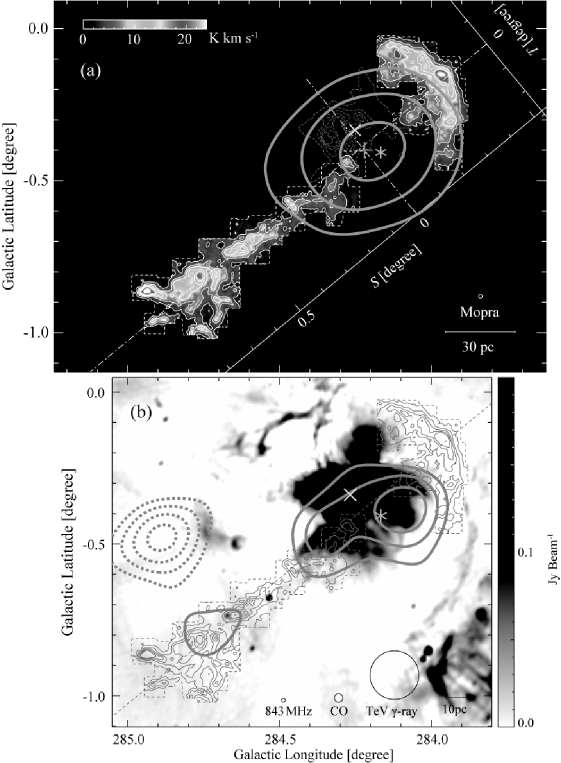
Figure 1: (a) The color image and white contours show the integrated intensity distributions of ¹²CO($J$=1–0) in a velocity range of 24 – 32 km s^-1. The white contours are drawn every 3.3 K km s^-1 ($=4\sigma$) up to 5 levels. The orange contours show significance levels of the HESS J1023$-$575 at a energy range of 0.7 – 2.5 TeV started from $7\sigma$ in step of $3\sigma$. The orange plus is the gravity center of the TeV $\gamma$-ray emission. The magenta contours show the radio continuum emission at 843 MHz drawn every 0.5 Jy beam^-1 from 0.2 Jy beam^-1. $S$ axis is taken along the jet cloud and $T$ axis is taken vertical to $S$ axis (see Section 3.1.1). (b) The greyscale image shows the radio continuum emission at 843 MHz. The magenta contours show the ¹²CO($J$=1–0) (same as Figure 1a). The orange contours show the TeV $\gamma$-ray smoothed excess image above 2.5 TeV drawn every 5 excess arcmin^-2 from 20 excess arcmin^-2. The yellow x-marks and green asterisks in the both panels indicate the positions of Wd 2 and PSR J1023$-$5746, respectively.

Figure 1 shows the distribution of the jet and arc clouds toward Wd 2, where the ¹²CO($J$=1–0) intensity is integrated in a velocity range from 24 km s^-1 to 32 km s^-1. HESS J1023$-$575 is located between the two clouds. Paper I suggests that the jet and arc clouds are associated with HESS J1023$-5745$. The Fermi pulsar at 1.8–2.4 kpc (section 1) is unlikely associated with the jet and arc clouds located at 7.5 kpc (see section 3.2), and we do not consider that the pulsar is associated with the jet and arc clouds. There is another possible high energy source toward the jet, the radio continuum point source at ($l$, $b$)=(284$\fdg$55, $-$0$\fdg$70) (Figure 1b), whereas there is no additional support for its association with the jet cloud (see section 3.4). Therefore we shall hereafter adopt the assumption that the jet and arc clouds are associated with the HESS J1023$-$575. A straight line was determined by an intensity-weighted least-squares fitting to the jet and arc clouds and the following relation is obtained;

$$b\,\mbox{(degree)}=(-0.82\pm 0.01)l\,\mbox{(degree)}+(234.0\pm 3.3)\,\mbox{(degree)}.$$ (1)

This line shows a good positional agreement with the geometric center of the HESS J1023$-$575 within 0$\fdg$05. We adopt hereafter the coordinate system defined by the line; $S$ axis is taken along the jet cloud and $T$ axis is taken vertical to $S$ axis with the origin at $(l,b)=(284\fdg 23,-0\fdg 39)$ close to HESS J1023$-$575.

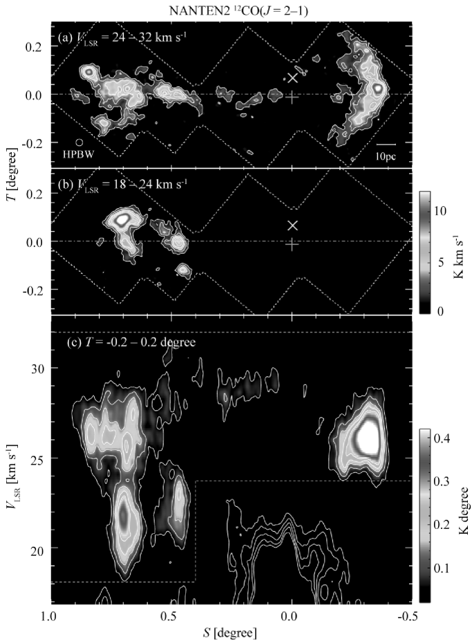
Figure 2: (a) Integrated intensity map of ¹²CO($J$=2–1). The integrated velocity range is 24 – 32 km s^-1. The contours are drawn up to 5 levels every 1.5 K km s^-1 (= $4\sigma$). The observed region is outlined by dashed lines. (b) Same as (a) but the integrated range is 18 – 24 km s^-1 and the contours are every 1.2 K km s^-1. (c) Position-velocity diagram integrated along the $T$ axis from $-0\fdg 2$ to $0\fdg 2$. The contours are drawn every 0.059 K degree (= $4\sigma$) up to 5 levels. The components drawn only with contours correspond to the GMC at 16 km s^-1 (outside of the dashed-line bouding box). The pluses and x-marks show the gravity center of HESS J1023$-$575 and center position of Wd 2, respectively.

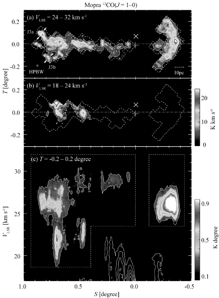
Figure 3: (a) Integrated intensity map of ¹²CO($J$=1–0). The integrated velocity range is 24 – 32 km s^-1. The contours are drawn up to 5 levels every 3.3 K km s^-1 (= $4\sigma$). The observed region is outlined by dashed lines. (b) Same as (a) but the integrated range is 18 – 24 km s^-1 and the contours are every 2.9 K km s^-1. (c) Position-velocity diagram integrated along the $T$ axis from $-$0$\fdg$2 to 0$\fdg$2. The contours are drawn every 0.16 K degree (= 4$\sigma$) up to 5 levels. The components drawn only with contours correspond to the GMC at 16 km s^-1 (outside of the dashed-line bouding box). The symbols are the same as in Figure 2.

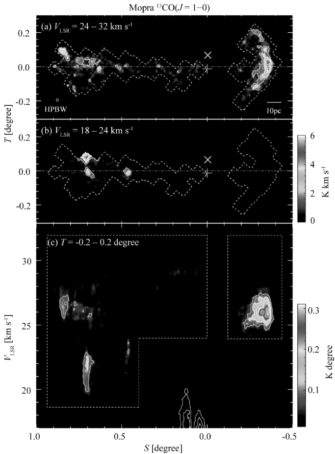
Figure 4: (a) Integrated intensity map of ¹³CO($J$=1–0). The integrated velocity range is 24 – 32 km s^-1. The contours are drawn up to 5 levels every 1.0 K km s^-1 (= 3$\sigma$) from 1.4 K km s^-1 (= 4$\sigma$). The observed region is outlined by dashed lines. (b) Same as (a) but he integrated range is 18 – 24 km s^-1 and the contours are every 0.9 K km s^-1 from 1.2 K km s^-1. (c) Position-velocity diagram integrated along the $T$ axis from $-$0$\fdg$2 to 0$\fdg$2. The contours are drawn every 0.20 K km s^-1 (= 3$\sigma$) from 0.26 K km s^-1 (= 4$\sigma$). The components drawn only with contours correspond to the GMC at 16 km s^-1 (outside of the dashed-line bouding box). The symbols are the same as in Figure 2

Figures 2, 3 and 4 show detailed distributions of the jet and arc clouds in the ¹²CO ($J$=2–1, 1–0) and ¹³CO ($J$=1–0), respectively. In each figure, panels (a), (b), and (c) show spatial distribution integrated in the two velocity ranges, 24 – 32 km s^-1 and 18 – 24 km s^-1, and position($S$)-velocity distribution, respectively. For the range 18 – 24 km s^-1 (each panel b) the ¹² CO ($J$=2–1) data cover the whole distributions while the $J$=1–0 data do not cover them. In each panel (a) of Figures 2–4, we see winding structures toward $S=$0$\fdg$1 – 0$\fdg$3 and $S=$0$\fdg$6 – 0$\fdg$9, whose kinematical details are shown in the next section. The arc cloud shows a nearly symmetric distribution with respect to the jet cloud axis.

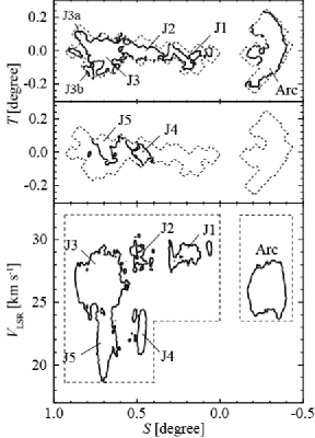
Figure 5: Finding chart for jet and arc clouds. The contours show the ¹²CO($J$=1–0) intensities integrated in the same ranges as Figure 2. The contours are drawn at 5$\sigma$ (4.2 K km s^-1 for the top panel and 3.6 K km s^-1 for the middle panel), and at 4$\sigma$ (=0.16 K degree) for the bottom panel.

Figure 3, the ¹²CO($J$=1–0) data at a higher spatial resolution, was used to define five features J1 – J5 for the jet cloud at the lowest contours in Figure 3 (c) and they are depicted in Figure 5. The jet cloud is divided into the two velocity ranges; the red-shifted features, J1, J2 and J3, and the blue-shifted features, J4 and J5. As shown in Figures 3 (a) and (b), J2 and J4 show good spatial coincidence, and J3 and J5 as well. Moreover, J3 and J5 are apparently connected in velocity in Figure 3 (c). Then, we shall consider two possibilities on the interpretation of J4 and J5. One is that the blue-shifted and red-shifted features are physically linked. If this is the case, the velocity span of the jet cloud becomes as large as $\sim$10 km s^-1 from the middle to the termination of the jet cloud. Another is that the blue-sifted and red-shifted features are located separately. If so, velocity widths of the individual features are $\sim$2 – 5 km s^-1 (Column 10 in Table 3). J3 seems to consist of two branches in the upper and lower parts in $T$. These two branches seem to bifurcate at $S\sim 0\fdg 65$ (Figures 3 a and 4 a) and have peaks at each eastern terminal positions named J3a and J3b (Figure 5). The arc cloud is in a velocity range from 24 km s^-1 to 29 km s^-1.

3.1.2 Details of the Jet Cloud

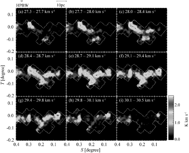
Figure 6: Velocity channel maps of J1 in ¹²CO($J$=1–0). The integrated velocity channel per map is 4 corresponding to 0.35 km s^-1. The contours are drawn every 0.70 K km s^-1 (=4$\sigma$). The observed region is outlined by dashed lines.

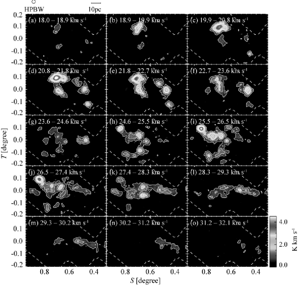
Figure 7: Velocity channel maps of J2 – J5 in ¹²CO($J$=2–1). The integrated velocity channel per map is 5 corresponding to 0.94 km s^-1. The contours are drawn every 0.50 K km s^-1 (=4$\sigma$) up to 5 levels. The observed region is outlined by dashed lines.

Figure 6 shows the velocity channel distributions of J1 in ¹²CO($J$=1–0). The component in the middle of J1 in $S=$ 0$\fdg$1 – 0$\fdg$30 is winding and shows a velocity gradient from $S=$ 0$\fdg$3 to $S=$ 0$\fdg$1. J1 appears to show a perpendicular component at $S=$0$\fdg$3 in Figures 6 (e) – (h). Figure 7 shows the velocity channel distributions of J2 – J5 in ¹²CO($J$=2–1). The bifurcation to the upper and lower features in J3 are seen in panels (h) and (i). The upper branch shows bending at $(S,T)=(0{\fdg}8,0{\fdg}05)$ and the lower branch also shows bending at ($S$, $T$)=(0$\fdg$7, $-$0$\fdg$1).

3.1.3 Details of the Arc Cloud and Evidence for the Counter Jet Cloud

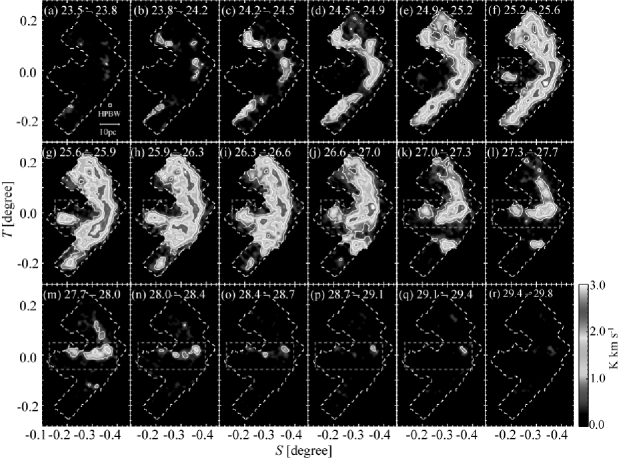
Figure 8: Velocity channel maps of arc in ¹²CO($J$=1–0). The integrated velocity channel per map is 4 corresponding to 0.35 km s^-1. The contours are drawn every 0.70 K km s^-1 (=4$\sigma$). The thick line boxes (magenta in a color version) are areas where the components of the western jet cloud are extracted as mentioned in Section 3.1.3. The observed region is outlined by dashed lines.

Figure 8 shows velocity channel distributions of the arc cloud in ¹²CO($J$=1–0). The integrated intensity in Figure 1 shows a clear crescent shape but the shape varies significantly in the individual velocity channels; e.g., the distribution in Figure 8 (d) is bent sharply. Another new aspect is that a feature elongated along the jet cloud axis is clearly seen in the velocity range from 25.2 km s^-1 to 29.4 km s^-1. This feature is seen in $S=-$0$\fdg$4 – $-$0$\fdg$2, showing a velocity gradient from 29.4 km s^-1 to 25.2 km s^-1 with $S$. We tentatively interpret this feature as a counterpart to the previously known jet cloud and shall call “western jet cloud” for convenience. In a similar manner, we call the jet cloud in the east of Wd 2 “eastern jet cloud” hereafter.

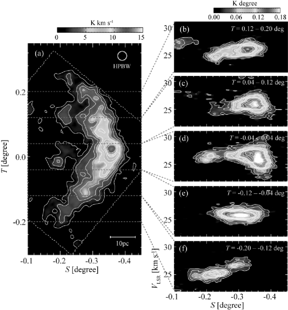
Figure 9: Position-velocity diagrams of arc integrated in various ranges of $T$. (a) Spatial intensity map of the arc cloud in ¹²CO($J$=2–1) integrated in 24 – 32 km s^-1. The contours are drawn every 1.5 K km s^-1 (=4$\sigma$). The thick line boxes (magenta in a color version) indicate the integrated regions of $T$ in the panels (b) – (f). (b) – (f) Position-velocity diagrams integrated along the direction of $T$. The contours are drawn every 0.016 K degree (=3$\sigma$) from 0.022 K degree (=4$\sigma$).

The western edge of the western jet cloud coincides with the peak of the arc cloud. Figure 9 shows more details of the arc cloud in the position-velocity diagrams. All the diagrams show small linewidth of less than 3 km s^-1 and show no systematic velocity shift in position. If the arc cloud is part of an expanding shell as suggested by its crescent shape, we expect a systematic change of velocity with the projected radius from the center. We suggest that the arc cloud may not be a shell but is a thin filamentary feature. In the appendix A, a schematic view of a typical position-velocity diagram for an expanding ellipsoidal shell is shown for comparison.

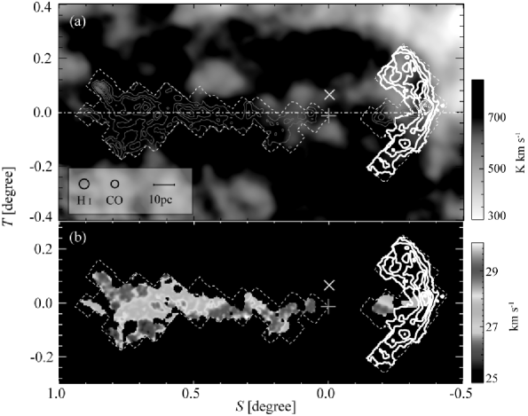
Figure 10: (a) Integrated intensities of eastern and western jet clouds in ¹²CO($J$=1–0) (magenta contours). The gray scale shows the integrated intensities of H I 21 cm line (McClure-Griffiths et al., 2005). The white contours show the integrated intensity of the arc cloud in ¹²CO($J$=1–0). All the data are integrated in a range of 24 – 32 km s^-1. The western jet cloud is extracted from the magenta boxes in Figure 8. The all contours are drawn every 3.3 K km s^-1 (=4$\sigma$). (b) Intensity-weighted first moment map of the eastern and western jet clouds. The contours are the same as in the panel (a). The symbols are the same as in Figure 2.

Figure 10 (a) shows the distribution of the eastern and western jet clouds and the arc cloud superposed on the H I distribution in the same velocity range from the Southern Galactic Plane Survey (McClure-Griffiths et al., 2005). Figure 10 (b) shows the intensity-weighted first moment map which indicates the barycentric velocity distribution in the eastern and western jet clouds and we see that the barycentric velocity increases from 26 km s^-1 to 29 km s^-1 in the eastern jet cloud and decreases from 28 km s^-1 to 26 km s^-1 in the western jet cloud from the center position of HESS J1023$-$575. The alignment of the two jet clouds seems good while the lengths of them are asymmetric; the eastern jet cloud has 100 pc in length and the western jet cloud has 40 pc in length at a distance of 7.5 kpc. We see a sign of an H I shell surrounding HESS J1023$-$575 as recognized in Paper I. The shell is elongated along the jet cloud axis with a size of 45 pc $\times$ 32 pc (Figure 10 a). Paper I suggests that the arc cloud is part of the H I shell formed under a compression related to HESS J1023$-$575, since HESS J1023$-$575 appears to be located toward the H I depression in the shell. We also confirm the elongated H I emission toward the eastern jet cloud (Paper I).

3.2 Distance of the Jet and Arc Clouds

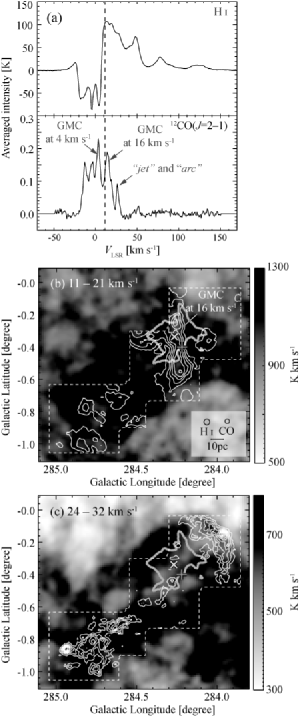
Figure 11: (a) Profiles of H I 21 cm (top) (McClure-Griffiths et al., 2005) and ¹²CO($J$=2–1) (bottom) lines toward RCW 49. The profiles are made by averaging in ($l$, $b$)=(284$\fdg$2 – 284$\fdg$4, $-$0$\fdg$4 – $-$0$\fdg$25) for H I and in ($l$, $b$)=(283$\fdg$8 – 285$\fdg$1, $-$1$\fdg$1 – 0$\fdg$0) for CO. Components of GMCs at the 4 km s^-1 and 16 km s^-1, and the jet and arc clouds are indicated in the CO profile. The dashed line shows the most redshifted velocity where the absorption occurs. (b) Integrated intensity map of H I 21 cm line in the velocity range of the GMC at 16 km  s^-1. The thin contours show the ¹²CO($J$=2–1) integrated intensities drawn every 5.8 K km s^-1 (=15$\sigma$) from 3.1 K km s^-1 (=8$\sigma$). (c) Integrated intensity map of H I 21 cm line in the velocity range of the jet and arc clouds. The thin contours are drawn every 1.5 K km s^-1 (=4$\sigma$). The symbols in panels (b) and (c) are the same as in Figure 2, and the thick contours (cyan in a color version) outline RCW49.

In order to test the distance of the relevant CO features, we show in Figure 11 (a) a comparison between the CO and H I line profiles. The H I should absorb the radio continuum of RCW 49 if the gas is in the foreground. The H I profile in Figure 11 (a) shows that only the blue-shifted features show signs of absorption toward the radio source, whereas the more red-shifted H I features show no sign of absorption (Figures 11 b and c). So, the GMC at 4 km s^-1 is located in front of RCW 49 and the GMC at 16 km s^-1 and the jet and arc clouds are behind RCW 49. There is no further hint about the physical linkage between the Wd 2-RCW 49-GMCs system and the jet-arc cloud system. Here we tentatively assume that the two systems are not physically associated. This assumption implies that HESS J1023$-$575 is not physically connected with Wd 2. We adopt a kinematic distance of the jet and arc clouds of $7.5_{-0.5}^{+0.2}$ kpc from the averaged intensity weighted velocity of 26.5 km s^-1 by using a flat-rotation model (Brand & Blitz, 1993), which is 2.1 kpc greater than that of the Wd 2-RCW 49-GMCs system. Here we assume that the galactic distance and rotation velocity at the Sun are 8.5 kpc and 220 km s^-1. The superscript and subscript values mean uncertainty of the distance which are derived by the kinematic distance of the most red-shifted and blue-shifted clouds among the arc and jet clouds in Table 3.

3.3 Physical Parameters of the Jet and Arc Clouds

3.3.1 The Radius, Mass, and Age of the Clouds

Radii and masses of the arc cloud and J1 – J5 at a distance of 7.5 kpc are summarized in Table 5. A radius $r$ of each cloud is derived by

$$r=\sqrt{\frac{A}{\pi}-{\left(\frac{\theta_{\rm HPBW}}{2}\right)}^{2}}\mbox{,}$$ (2)

where $\theta_{\rm HPBW}$ is the beam size in pc. $A$ is area where ¹²CO($J$=1–0) is detected above 4$\sigma$ in the integrated intensity in a range of 24 – 32 km s^-1 (J1 – J3) or ¹²CO($J$=2–1) in a range of 18 – 24 km s^-1 (J4 and J5; they are not fully covered in $J$=1–0). Mass is derived by

$$M=\mu m_{\rm H}\sum_{i}D^{2}\Omega N_{i}(\mathrm{H_{2}}),$$ (3)

where $\mu$ is the mean molecular weight per H molecule, $m_{\rm H}$ the proton mass, $D$ the distance, $\Omega$ the solid angle of one pixel, and $N_{i}(\rm H_{2})$ the column density of each pixel. We use $\mu=2.8$ by adopting the helium abundance of 20% to the molecular hydrogen. The column density is estimated by using a conversion factor called as X-factor $X_{\rm CO}$ from the integrated intensity of ¹²CO($J$=1–0), $W(\rm CO)$, to the column density as $N({\rm H_{2}})=X_{\rm CO}\cdot W({\rm CO})$. For J4 and J5 we converted ¹²CO($J$=2–1) integrated-intensities into ¹²CO($J$=1–0) intensities with $J$=1–0/$J$=2–1 ratios of 0.43 (J4) or 0.47 (J5). In the present work we adopt $1.6\times 10^{20}$ cm^-2 (K km s^-1)^-1 as the X-factor (Hunter et al., 1997) obtained by EGRET observations instead of $2.0\times 10^{20}$ cm^-2 (K km s^-1)^-1 (Bertsch et al., 1993) used in Paper I, since the former was derived with CO data by taking into account a correction factor of 1.22 in the calibration (Hunter et al., 1997). We note that values of the X-factor derived by various works based on $\gamma$-ray observations, infrared observations, and so on (e.g., Bloemen et al., 1986; Reach et al., 1998; Dame et al., 2001) are in a range of $(1\mbox{--}3)\times 10^{20}$ cm^-2 (K km s^-1)^-1. Therefore, the obtained molecular masses may include $\sim$50 % uncertainty.

From Table 5 the molecular mass of the eastern jet cloud (EJ), that of the western jet cloud (WJ), and that of the arc cloud are estimated to be $M({\rm EJ})=5.6\times 10^{4}M_{\sun}$, $M({\rm WJ})=2.9\times 10^{3}M_{\sun}$, and $M({\rm arc})=2.5\times 10^{4}M_{\sun}$, respectively. The H I mass for an area $1\fdg 5\times 0\fdg 8$ shown in Figure 10 (a) amounts to $1.5\times 10^{5}M_{\sun}$ and the molecular gas corresponds to $\sim$60% of the atomic mass. These values differ from those in Paper I mainly because of the distance revised and the different X-factor.

Crossing timescale of a molecular cloud obtained by dividing the molecular cloud size by the linewidth is often used as a measure of typical cloud timescale, since this means a time in which the cloud can significantly alter its morphology. The width of the jet and arc clouds is $\sim$5 – 10 pc, and their linewidths $\Delta V_{\mathrm{comp}}$ are 2 – 5 km s^-1 (Table 2). The crossing timescale of the jet and arc clouds is estimated to be in the order of a few Myr.

3.3.2 The Line Intensity Ratios; the ¹²CO ($J$=2–1, 1–0) and ¹³CO ($J$=1–0) Transitions

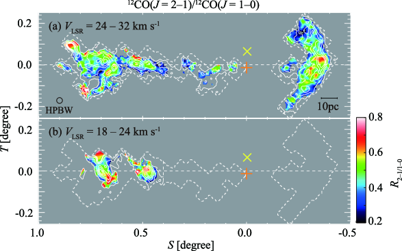
Figure 12: Integrated intensity ratio maps of ¹²CO($J$=2–1) to ¹²CO($J$=1–0), $R_{\rm 2-1/1-0}$. The integrated ranges are written in the panels. Only pixels where the integrated intensities exceeding 4$\sigma$ in both of the lines are shown. (a) The contours are the ¹²CO($J$=1–0) integrated intensities every 3.3 K km s^-1 (=4$\sigma$) up to 4 levels. (b) The contours are the ¹²CO($J$=1–0) integrated intensities every 2.9 K km s^-1 (=4$\sigma$) up to 4 levels. The symbols are the same as in Figure 2.

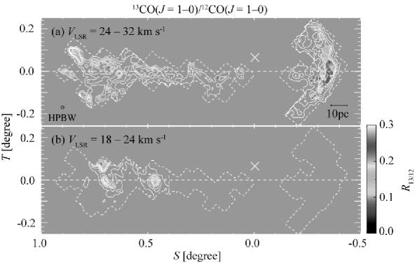
Figure 13: Integrated intensity ratio maps of ¹³CO($J$=1–0) to ¹²CO($J$=1–0), $R_{\rm 13/12}$. The integrated ranges are written in the panels. Only pixels where the integrated intensities exceeding 4$\sigma$ in both of the lines were shown. The contours and symbols are the same as in Figure 12.

Ratios between different $J$ transitions and isotopes reflect excitation conditions and density in the molecular clouds. The excitation of molecular transitions depends on the temperature and density in the molecular gas. The line intensity ratio of the three transitions are summarized in Figures 12 and 13. The 1–0 data were Gaussian smoothed to a 90″ beam size. Figure 12 shows distributions of the integrated intensity ratio of ¹²CO($J$=2–1) to ¹²CO($J$=1–0), $R_{2-1/1-0}$, where the both lines are detected above $4\sigma$. Although the average of the ratio is 0.45, the ratio exceeds 0.6 at the peak position of the arc cloud, at J3a and J3b, and at the peak positions of J4 and J5. The ratio is high at the edges of the clouds in some places, which could be artifacts due to low S/N ratios. Figure 13 shows spatial distributions of the integrated intensity ratio of ¹³CO($J$=1–0) to ¹²CO($J$=1–0), $R_{13/12}$, where both lines are detected above 4$\sigma$. $R_{13/12}$ reflects molecular column density distributions. The ratio is enhanced to be around 0.25 in the arc cloud, J3a and the two peaks of J5. It implies the column density becomes relatively higher at these positions than the rest.

3.3.3 The LVG Analysis

In order to estimate kinetic temperature and number density of the molecular clouds, we carried out the LVG (large velocity gradient) analysis (Goldreich & Kwan, 1974) for points where the ¹³CO($J$=2–1) pointed observations were made. The employed model assumes a spherically symetric cloud where kinetic temperature $T_{\rm kin}$, number density $n({\rm H}_{2})$ and radial velocity gradient $dv/dr$ are taken to be uniform. We changed $T_{\rm kin}$ and $n({\rm H}_{2})$ within $T_{\rm kin}=6$ – 500 K and $n({\rm H}_{2})=10$ – $10^{6}$ cm^-3, where we fix $X/(dv/dr)$ for a cloud size of a few pc and a linewidth of a few km s^-1. For an isotope ratio of [¹²C]/[¹³C], we adopt 75 at the Galacto-centric distance of $\sim$9 kpc (Milam et al., 2005).

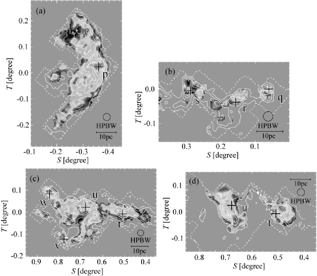
Figure 14: Closeup of Figure 12. The pluses point positions where the LVG analyses are performed.

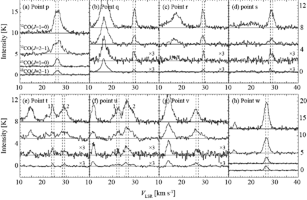
Figure 15: Spectra of ¹²CO($J$=1–0), ¹³CO($J$=1–0), ¹²CO($J$=2–1), and ¹³CO($J$=2–1) where LVG analyses are performed. The ¹³CO($J$=1–0) and ¹³CO($J$=2–1) spectra in (b) – (g) are multiplied by a factor of 3. The vertical broken lines show the integrated range of 1 km s^-1 around the barycentric velocities used in the LVG analyses.

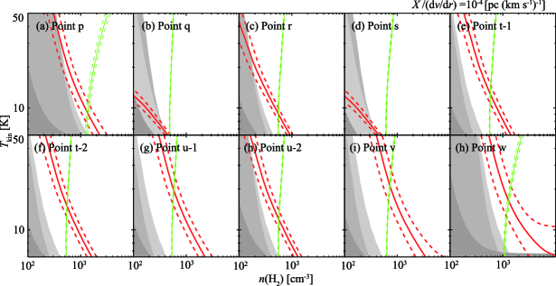
Figure 16: Number density and kinetic temperature curves obtained by LVG analyses. The thick and thin (red and green in a color version) lines are the observed ratios of ¹³CO($J$=2–1)/¹³CO($J$=1–0) and ¹³CO($J$=2–1)/¹²CO($J$=2–1), respectively. The dashed lines indicate errors from calibration errors of each line, of 10% for ¹²CO($J$=2–1) and ¹³CO($J$=1–0) and 20% for ¹³CO($J$=2–1). The gray zones indicate areas where the filling factors become above 1 (dark: ¹²CO $J$=2–1, middle: ¹³CO $J$=1–0, and light: ¹³CO $J$=2–1; see Section 3.3.3).

We chose eight local peaks p – w of ¹²CO($J$=1–0) for the ¹³CO($J$=2–1) pointed observations. Their positions and line profiles are shown in Figures 14 and 15, respectively. We used averaged intensity ratios around the barycenter velocity with a 1 km s^-1 window in the LVG analysis. We chose two combinations of the ratios among ¹²CO($J$=2–1), ¹³CO($J$=1–0) and ¹³CO($J$=2–1). We did not use the ¹²CO($J$=1–0) line since it is generally optically thick and may sample only the nearside lower density gas (e.g., Mizuno et al., 2010). The averaged intensities and barycentric velocities are listed in Columns (6) – (9) of Table 6. For the points t and u, where spectra show double components, we estimate $T_{\rm kin}$ and $n({\rm H}_{2})$ for each component. $X/(dv/dr)$ is set to $10^{-4}$ pc (km s^-1)^-1 with the canonical [CO]/[H₂] abundance of $10^{-4}$ (Frerking et al., 1982). The results for $T_{\rm kin}$ and $n({\rm H}_{2})$ are shown in Figure 16. The curves represent each observational line intensity ratio. We also estimated a beam filling factor through dividing the observed line intensity by the calculated line intensity for the three transitions. If this factor becomes greater than 1, the parameter will not be realized (gray areas in Figure 16).

The density is estimated to be less than 10³ cm^-3 except for the points p, v, and w. At the peak position of the arc cloud and J3, i.e. the points p and w, the density increases to $\sim$10^3.1 cm^-3. The arc cloud and J1, i.e., points p – s, have low temperature below $\sim$10 K, whereas the other positions in the jet cloud, especially v and w, have higher temperatures of $\sim$20 K in a range of 12 – 28 K.

3.4 Star Formation in the Jet and Arc Clouds

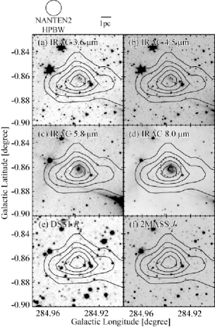
Figure 17: Near – middle infrared (Spitzer/IRAC 3.6, 4.5, 5.8, 8.0 µm and 2MASS $J$ band) and visible (DSS1 $R$ band) images toward J3a. The contours are the ¹³CO($J$=1–0) integrated intensity drawn every 1.0 K km s^-1 (=3$\sigma$) from 1.4 K km s^-1 (=4$\sigma$). The small circle and large dashed-line circle show positions of point sources in 9.0 µm from AKARI IRC PSC and in 160 µm from AKARI FIS BSC. The diameters of the circles indicate each angular resolution (FWHM) of 5$\farcs$5 in 9.0 µm (Onaka et al., 2007) and 61″ for in 160 µm (Kawada et al., 2007), respectively.

We have searched for young objects in the IRAS point source catalog and the Siptzer/IRAC data from Spitzer Heritage Archive. As a result, we find one possible candidate for a young star toward J3a as shown in Figure 17. The source is detected significantly toward the ¹³CO ($J$=1–0) peak as a nebulous extended source at 5.8 µm and 8.0 µm. This source is possibly identical with sources detected at 9 µm by the AKARI IRC Point Source Catalogue (IRC PSC) (Kataza et al., 2010) and 160 µm by AKARI FIS Bright Source Catalogue (FIS BSC) (Yamamura et al., 2010), whereas no counterpart can be confirmed in DSS1 Red band, 2MASS $J$ band (Figures 17 e and f) and radio continuum at 843 MHz (Figure 1b). The flux densities of the AKARI sources are summarized in Table 7. By the lack of infrared data at the other wavelengths, especially far-infrared, a detailed analysis of the evolutionary stage (e.g., Class 0–III) and estimation of the mass of the young star remain as the future work. It takes $\sim$Myr for such usual low-mass star formation, as is consistent with the crossing time of the jet cloud of a few Myr.

Figure 1b shows a radio continuum image at 843 MHz from the 2nd epoch Molonglo Galactic Plane Survey (MGPS-2) by the Molonglo Observatory Synthesis Telescope (MOST) (Murphy et al., 2007) with the integrated intensity of the jet and arc clouds in ¹²CO ($J$=1–0) overlaid. The radio emission is dominated by the thermal free-free emission of the H II region RCW 49. The H II region shows a ridge extending toward the southeast nearly along the jet cloud axis, while its connection with the jet cloud is not clear. We find no significant radio source except for a few unresolved compact sources in the direction of the jet clouds at $(l,b)=$(284$\fdg$53, $-0\fdg 68$) and $(l,b)=$(284$\fdg$68, $-0\fdg 74$). However, no counterparts of these radio sources are seen in the infrared data such as the Siptzer/IRAC, which show the hot dust heated by nearby H II regions. In addition, $R_{2-1/1-0}$ in Figure 12 is not high toward the position of the radio sources, and we find no significant velocity variations around these two radio sources at $S\sim 0\fdg 45$ and $0\fdg 56$ as seen in Figures 2 and 3. Therefore, it is likely that the radio sources are not compact H II regions associated with the jet cloud and may be extragalactic. To summarize, the jet and arc clouds as a whole are not active in star formation.

3.5 Comparison with the TeV $\gamma$-Rays

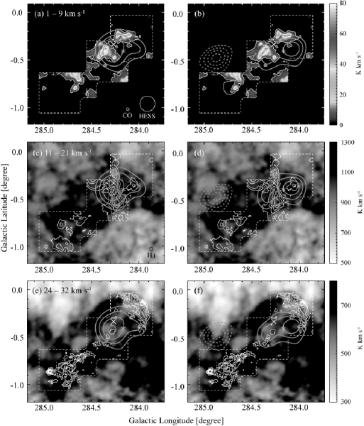
Figure 18: Comparison between TeV $\gamma$-ray distribution and ISM gas. The thick (orange in a color version) contours are the TeV $\gamma$-ray smoothed excess images (as same as Figure 2 in H.E.S.S. Collaboration, 2011b). The left side panels (a, c, and e) are at the low energy band (0.7 – 2.5 TeV), and the right side panels (b, d, and f) are at the high energy band (above 2.5 TeV). The contours are drawn every 10 excess arcmin^-2 from 40 excess arcmin^-2 for the low energy band, and every 5 excess arcmin^-2 from 20 excess arcmin^-2 for the high energy band. The dashed contours show HESS J1026$-$582. (a) and (b) The images and thin contours show the integrated intensities of ¹²CO($J$=2–1) in the velocity range of the GMCs at 4 km s^-1. The contours are drawn every 14 K km s^-1 (=40$\sigma$) from 2.8 K km s^-1 (=8$\sigma$). (c) and (d) The gray scale shows the integrated intensities of the H I 21 cm line in the velocity range of the GMCs at 16 km s^-1. The thin contours are the integrated intensities of ¹²CO($J$=2–1) drawn every 5.8 K km s^-1 (=15$\sigma$) from 3.1 K km s^-1 (=8$\sigma$). (e) and (f) The gray scale shows the integrated intensities of the H I 21 cm line in the velocity range of the jet and arc clouds. The thin contours are the integrated intensities of ¹²CO($J$=2–1) drawn every 1.5 K km s^-1 (=4$\sigma$). The symbols are the same as in Figure 1.

In order to see if the $\gamma$-rays show spatial correspondence with the molecular gas, we show a comparison of the TeV $\gamma$-ray distribution of HESS J1023$-$575 (H.E.S.S. Collaboration, 2011b) with the CO at three velocity intervals in Figure 18. We show the two energy ranges of 0.7 – 2.5 TeV (low-energy band) and of above 2.5 TeV (high-energy band). A source HESS J1026$-$582 shown by the dashed line is supposed to be a PWN powered by a pulsar PSR J1028$-$5819 at a distance 2.3 kpc and is not associated with Wd 2 (H.E.S.S. Collaboration, 2011b).

We find that the major parts of the two GMCs at 1 – 21 km s^-1 (Furukawa et al., 2009) are within the lowest contour of the $\gamma$-rays (Figures 18 a – d). Considering the relatively coarse resolution of H.E.S.S. $\sim 0\fdg 07$, the two GMCs may be possible candidates for the $\gamma$-ray production via the hadronic process (Fujita et al., 2009b; H.E.S.S. Collaboration, 2011b). On the other hand, the jet and arc clouds are located around HESS J1023$-$575, showing an anti-correlation with the $\gamma$-ray distribution, whereas there is relatively bright H I gas toward the $\gamma$-rays (Figures 18 e and f). The target protons may be mostly atomic, if the $\gamma$-rays are of the hadronic origin from the jet and arc clouds region. The distribution at the high-energy TeV $\gamma$-ray band shows a hint of elongation along the jet cloud direction, suggesting that the $\gamma$-ray source may be related with the jet cloud. In the high energy band, another faint source is detected about 4$\sigma$ but less than 5$\sigma$ toward the jet cloud at $(l,b)=(284\fdg 7,-0\fdg 8)$, possibly suggesting association with the jet cloud. Toward this new $\gamma$-ray source only a radio source at $(l,b)=$(284$\fdg$68,$-0\fdg 74$) in Figure 1b exists within the 4$\sigma$ contour. However, there is no identification of the radio source in Véron-Cetty & Véron (2010) and Manchester et al. (2005) so far. The radio source may also be a possible candidate of the new $\gamma$-ray source counterpart, but this cannot be confirmed. We discuss further on the $\gamma$-ray origin toward the Wd 2 region in Section 4.4.

4 DISCUSSION

4.1 The Jet and Arc Clouds Associated with HESS J1023$-$575

Most of the individual jet and arc clouds have density, temperature and linewidth similar to the other Galactic molecular clouds like the Taurus dark cloud. The highly filamentary and elongated nature of the jet cloud having 100 pc length and several pc width may, however, be fairly exceptional among the Galactic clouds; the typical filamentary clouds have shorter projected lengths of 10 – 50 pc (e.g., Taurus: Mizuno et al. 1995; Chamaeleon: Mizuno et al. 2001; L1333: Obayashi et al. 1998). It is also notable that the arc cloud having $10^{4}$ $M_{\sun}$ shows an outstanding crescent shape; we have not yet been informed on such a well-defined arc-like cloud to date in the literature. If the blue-shifted features J2 – J4 and the red-shifted features J3 – J5 are physically connected, part of the jet cloud has a velocity span of $\sim$10 km s^-1. These broad features may not be gravitationally bound by the self-gravity for the cloud mass and size of $\sim 10^{4}$ $M_{\sun}$ and $\sim$10 pc, respectively (Columns 3 and 4 in Table 5). We shall discuss the origin of the jet and arc clouds later into more detail.

The molecular clouds toward Wd 2 consist of two groups of different velocity ranges, $-10$ – 20 km s^-1 and 20 – 30 km s^-1. The former group includes the two parent GMCs at 4 km s^-1 and 16 km s^-1 which show tight correlation with Wd 2 and RCW 49 as verified by the high line intensity ratio of ¹²CO ($J$=2–1)/($J$=1–0) around 1.0, corresponding to kinetic temperature above $\sim$30 K (Ohama et al., 2010). The latter group consisting of the jet and arc clouds shows no enhanced line ratio of ¹²CO ($J$=2–1)/($J$=1–0) or higher temperature toward RCW 49 (points q and r in Figure 14). We therefore infer that the jet and arc clouds are not close enough to be heated by RCW 49 or Wd 2 and this geometrical separation is consistent with the velocity difference of the two groups by $\sim$20 km s^-1 and with a kpc-scale separation between them.

By comparison with the TeV $\gamma$-ray distributions in Figure 18, we suggest that the jet and arc clouds are physically associated with HESS J1023$-$575 and are located at a distance of 7.5 kpc, larger than that of Wd 2 of 5.4 kpc. A consequence of this location is that the scenarios for $\gamma$-rays production due to the stellar winds/blister energized by the stellar cluster may not be appropriate.

In the followings, we shall discuss on 1) the formation of the jet cloud, 2) the formation of the arc cloud, and 3) the possible origin for the $\gamma$-ray source.

4.2 Formation of the Jet Cloud

Paper I presented a hypothesis about the formation mechanism of the jet cloud as follows: first, a high-energy jet driven by an anisotropic SN explosion or by a microquasar is injected into the ambient atomic or molecular gas. The gas is then compressed cylindrically by the shock fronts due to the high-energy jet. Eventually, molecular clouds with a linear shape were formed in the compressed gas.

Asahina et al. (2013) carried out magneto-hydro-dynamical (MHD) numerical simulations of the interaction between a high-energy jet and ambient ISM. As the initial conditions, they assume H I gas in the Cold Neutral Medium (CNM) phase with temperature of $\sim$200 K and density of $\sim$10 cm^-3. The velocity and radius of the high-energy jet were assumed to be 200 km s^-1 and 1 pc, which aims at modeling the high-energy jet slowed down in the interaction with the ISM, or, the high-energy jet launched by a rotating disk much larger than the size of the compact object. Such a jet is actually consistent with SS 433, the microquasar having the X-ray jet (Brinkmann et al., 1996) extending by $\sim$50 pc from the central object at a distance of $\sim$3 kpc (Dubner et al. 1998; a different distance of 5.5 kpc is estimated by Hjellming & Johnston 1981; Blundell & Bowler 2004). When the high-energy jet is injected, the H I gas is compressed and heated up, where this heating will be on a scale much smaller than pc. In the calculations, a cooling function defined in Inoue et al. (2006) is adopted, whereas the self-gravity is not included. By the cooling effect, the compressed gas finally becomes cool and dense with temperature of $\sim 50$ K and density of $\sim 50$ cm^-3 due to the thermal instability. It is possible that such cool and dense gas can be transformed by self-gravity into the molecular clouds which trace the trajectory of the high-energy jet. The column density of the H I gas is actually enhanced toward the jet cloud as shown in Figure 10 (a). Enhancement of the H I gas column density along the jet cloud axis is also seen in SS 433 and in another candidate for the molecular jet at $(l,b)=$(348$\fdg$5, $-2\arcdeg$ – $+2\arcdeg$) (Yamamoto et al., 2008). Asahina et al. (2013) have shown that the compressed gas has an expansion velocity of $\sim$2 km s^-1 perpendicular to the propagation axis of the high-energy jet. This is consistent with the full linewidths of the individual jet clouds of $\sim 2$ – 5 km s^-1 (Column 10 in Table 3). Although the anisotropic jet-like SN explosion is suggested in Paper I, there is no numerical simulation on such a process. We shall not discuss this alternative further in the present work. The numerical simulations by Asahina et al. (2013) may also be applicable to the anistropic jet-like SN explosion if the physical parameters such as the jet speed and the shock strength are similar to those in Asahina et al. (2013).

The interaction may cause heating of the gas, while the cooling by molecule lines is fairly rapid like $10^{4}$ yrs or less for density around $10^{3}$ cm^-3 or higher as derived in the present LVG analysis shown in Figure 16 and Table 6 (e.g., Goldsmith & Langer, 1978). In Section 3.3.2 the distribution of the line intensity ratio ¹²CO ($J$=2–1)/($J$=1–0) is shown in Figure 12, which indicates that the kinetic temperature may become higher in a few places in the jet cloud, i.e., toward J3a, J3b, J4 and J5. J3a and J3b show line ratios of 0.6 – 0.8 implying temperature of $\sim$20 K, significantly higher than the usual temperature of the molecular gas, 10 K, with no extra local heating. We also note that parts of J4 and J5 show somewhat higher line intensity ratios above 0.7, and they may suggest some extra shock heating due to the high-energy jet. A possibility is that J4 and J5 accelerated by the high-energy jet are still interacting with other molecular gas and have been causing a shock heating until now. J3a has a sign of recent star formation as shown in Section 3.4 and it may be an alternative that this young star is radiatively heating J3a, while the star with no thermal radio continuum source (Figure 1b) may not be luminous enough to explain the temperature excess.

The winding shape of the jet cloud in a few places is intriguing (Sections 3.1.1 and 3.1.2) and may give some hints on the details of the interaction of the high-energy jet. For instance, the winding shape may trace MHD instability of a helical shape in the propagating magnetized jet. Such helical patterns are in fact observed in MHD numerical simulations of the high-energy jet (e.g., Nakamura et al., 2001). It is also interesting to see the time variation of the high-energy jet; a question is if the jet is impulsive or intermittent over a time scale of Myr. It may be difficult to explain the winding shape of the remnant molecular gas by a continuous helical flow of the high-energy jet material, which may destroy the helical pattern even if it is once formed. Because of this, impulsive or intermittent jet may be favorable.

4.3 Formation of the Arc Cloud

We shall then discuss the formation of the arc cloud. The present work has shown two new detailed aspects of the arc cloud. One is the western jet cloud identified toward the arc cloud, which seems to be terminated in the middle of the arc cloud, and the other is that the arc cloud shows symmetry with respect to the jet cloud axis. The arc cloud is also part of the H I shell as suggested in Paper I (see Figure 3 of Paper I).

An obvious explanation of the formation of the arc cloud is an SN explosion. In order to test this possibility we calculate the radius and mass of a shell formed due to an SN explosion by using equations in Appendix B. We shall assume a uniform ambient density, $10^{51}$ erg for the total mechanical energy of the SN explosion, and $10^{4}$ km s^-1 for the initial velocity of the shock, and calculate the parameters when the shock velocity decreases to the sound speed of typical temperature $\sim$100 K in the CNM, i.e. $\sim$1 km s^-1. According the calculations, when the ambient density is $\sim$1 cm^-3, the radius reaches 45 pc, which is consistent with that of the arc cloud at the distance of 7.5 kpc, for an age of $5\times 10^{4}$ yr. But the mass of the shell is only $9.1\times 10^{3}$ $M_{\sun}$, which is much smaller than the observed total mass of the arc cloud and H I shell $\sim 2\times 10^{5}$ $M_{\sun}$. To explain the mass of the arc cloud and H I shell, the ambient density of 15 cm^-3 is required, but, if so, the radius of an SNR becomes smaller as 34 pc for an age of $1\times 10^{5}$ yr. If the mechanical energy of the SN explosion is higher by a factor of 5, i.e., $5\times 10^{51}$ erg, both of the radius and mass of the arc cloud and H I shell can be explained even if the ambient density is 15 cm^-3. However, we should note that the calculations include many assumptions such as the uniform density, and the real situations may be more complicated. In addition, we have another problem of the column density contrast between the H I shell and the CO arc of about 1:10. It is questionable if the shell can expand to a similar radius for such density contrast. Therefore, we have to note that there are difficulties on the SN explosion to form the arc cloud.

As an alternative possibility of the formation mechanism of the arc cloud, we shall consider the interaction of the high-energy jet. The shape of the arc cloud is symmetric about the jet cloud axis, and the western jet cloud is elongated along the jet cloud axis. These properties suggest that the high-energy jet is tightly related to the formation of the arc cloud. Asahina et al. (2013) shows that the high-energy jet forms a bow shock in the adiabatic case. This suggests that, if the cooling is not dominant, the interaction may form a bow-shock like arc cloud at the edge of the western jet cloud. A ring-like radio structure similar to the arc cloud is observed around the microquasar Cyg-X1 (Gallo et al., 2005) and it is believed that the interaction between the high-energy jet and surrounding ISM created the structure. This radio emission originates from the bremsstrahlung from hot plasma, and some atomic lines such as H$\alpha$ and O III are also detected in the radio ring (Russell et al., 2007). If such hot gas cools down, molecular gas like the arc cloud may be formed. It is desirable that a further study is devoted to pursue the formation of the bow shock driven by the high-energy jet via numerical simulations in order to have a better insight into the bow shock formation. It is puzzling that the eastern and western jet clouds are fairly asymmetric in the sense that the eastern jet cloud is extended by a factor of 2.5 than the western jet cloud. The arc cloud suggests that the ISM in the western region is more massive than in the eastern region of Wd2 and may offer a possible explanation on the asymmetry.

4.4 Origin of the $\gamma$-Rays

We shall discuss the origin of the $\gamma$-rays of HESS J1023$-$575 in the present framework based on the jet and arc clouds. Since the $\gamma$-rays are distributed inside the H I shell, where there is no CO, in Figure 18, the H I gas is considered as the targets for CR protons, if the $\gamma$-rays are of the hadronic origin. The basic timescales of the hadronic process are the cooling timescale and the diffusion timescale. Density of the target protons in a sphere with radius of 0$\fdg$18 centered at the central position of HESS J1023$-$575 is derived to be $n_{\mathrm{inner}}$=12 cm^-3 at 7.5 kpc. Then, the cooling time scale due to the pp-interaction is given as follows (Gabici et al., 2009),

$$t_{\rm pp}=5\times 10^{6}\,{\rm yr}\left(\frac{n_{\rm inner}}{12\,{\rm cm}^{-3}}\right)^{-1}.$$ (4)

Also, since the radius of the $\gamma$-ray extent (0$\fdg$18) becomes $R_{\mathrm{inner}}$=24 pc at 7.5 kpc, the diffusion time scale of CR protons is given as follows (Gabici et al., 2009),

$$t_{\rm diff}=2\times 10^{4}\,{\rm yr}\left(\frac{\chi}{0.01}\right)^{-1}\left(\frac{R_{\rm inner}}{24\,{\rm pc}}\right)^{2}\left(\frac{E_{\rm p}}{10\,{\rm TeV}}\right)^{-0.5}\left(\frac{B}{10\,{\mu\rm G}}\right)^{0.5},$$ (5)

where $E_{\mathrm{p}}$=10 TeV is the CR proton energy, the magnetic field strength $B$ is assumed to be 10 $\mu$G and $\chi$ means the deviation from typical diffusion coefficient in the Galaxy. If an SN explosion occurred in the past, magnetic turbulence will be enhanced and yield low $\chi$ value such as 0.01. Equations (4) and (5) show that the diffusion timescale is much shorter than the other timescales although the cooling timescale is consistent with the crossing timescale of the jet and arc clouds. Therefore, the particle acceleration should occurs within $\sim 10^{4}$ yr in the hadronic scenario.

Most known TeV $\gamma$-ray sources in the Galaxy are either SNRs or PWNe. The bright TeV $\gamma$-ray SNRs are all young SNRs of 1000 – 2000 yrs (RX J1713.7$-$3946: Aharonian et al. 2006b, 2007c; RX J0852.0$-$4622: Aharonian et al. 2007b; RCW86: Aharonian et al. 2009 and HESS J1731$-$347: H.E.S.S. Collaboration 2011a) and the TeV $\gamma$-ray PWNe are younger than $\sim 10^{5}$ yr as estimated by the spin-down rate (Kargaltsev & Pavlov, 2010). On the other hand, toward Wd 2, no SNRs are known, and conclusive evidence of a PWN has not been found. Even if HESS J1023$-$575 is either an SNR or PWN associated with the jet and arc clouds, lifetime of the relativistic particles accelerated at the SNR or PWN are much shorter than the age of the jet and arc clouds of $\sim$Myr suggested by the crossing timescale and the existence of star formation. If an SN which is a progenitor of the SNR or PWN created the jet and arc clouds in $\sim$Myr ago, the relativistic particles from the SNR or PWN must have already cooled or escaped in the first $\sim 10^{4}$ yr, and cannot emit the TeV $\gamma$-rays at present. The same reasoning will be applied to the hypothesis, an anisotropic SN explosion (Sections 4.2 and 4.3). Therefore, an SNR or a PWN is not likely as the origin for HESS J1023$-$575, if the jet and arc clouds and HESS J1023$-$575 are due to a single object.

The only remaining possible candidate for the $\gamma$-ray origin is the CRs accelerated in microquasar jet interacting with the ambient ISM. Particle acceleration of the termination shock of microquasar jet interacting with the ISM has been theoretically studied and it is shown that such interaction can produce CRs (e.g., Bosch-Ramon et al., 2005). The microquasar may have a potential to be active over $\sim$Myr, even intermittently, which favors the molecular cloud formation. Figures 18 (e) and (f) indicate that there exists relatively dense H I gas beyond the TeV $\gamma$-ray extent, suggesting that the spatial extent of the CR protons should be similar to that of the TeV $\gamma$-rays. The CRs may be confined by the dense H I shell and the arc cloud. Total energy of the CR protons estimated from the TeV $\gamma$-ray luminosity $L_{\mathrm{\gamma}}$(1–10 TeV) is given as follows;

$$W_{\mathrm{p}}\left(10\mbox{--}100\,{\rm TeV}\right)\sim 7\times 10^{48}\,{\rm erg}\left(\frac{t_{\rm pp}}{5\times 10^{6}\,{\rm yr}}\right)\left[\frac{L_{\gamma}\left(1\mbox{--}10\,{\rm TeV}\right)}{4.5\times 10^{34}\,{\rm erg\,s}^{-1}}\right].$$ (6)

Here, we use the $\gamma$-ray luminosity $4.5\times 10^{34}$ erg s^-1 derived at 7.5 kpc. If this energy is released during the diffusion time of $\sim$10⁴ yr, averaged power injected to the CR protons becomes $\sim 2\times 10^{37}$ erg s^-1 which is consistent with the theoretical work (Bosch-Ramon et al., 2005).

The total radio fluxes of the known microquasors (e.g., SS 433, LS I +61 303, LS 5039 and Cyg X-3) located within several kpc are measured to be 867 mJy, 42 mJy, and 87 mJy at 1.4 GHz, respectively (Paredes et al., 2002). On the other hand, the observed flux toward RCW49 is larger than 1 Jy beam^-1 at 843 MHz as seen in Figure 1. It is thus hard to distinguish a microquasar from the strong and complicated radio emission, if it not exceptionally bright like SS 433.

We should note that the physical characteristics of HESS J1023$-$575 are different from those of the other microquasars in the Galaxy. The $\gamma$-rays toward microquasars have been discovered at Cyg-X1 (Albert et al., 2007; Sabatini et al., 2010) and Cyg-X3 (Fermi LAT Collaboration, 2009). They are compact (unresolved) and have a time modulation or flares. The $\gamma$-ray binaries, such as LS 5039 (Aharonian et al., 2006a; Abdo et al., 2009b) and LS I+61°303 (Albert et al., 2006; Acciari et al., 2008; Abdo et al., 2009a), which are thought to be candidates of microqusars, also have compact features and time modulations. We infer that the $\gamma$-ray radiation mechanisms are different between HESS J1023$-$575 and the other microquasars in physical conditions such as density of the ambient matter.

As shown in Section 3.5, the faint $\gamma$-ray emission was discovered toward the jet cloud J3 at $(l,b)=(284\fdg 7,-0\fdg 8)$ by the new H.E.S.S. observations. A counterpart such as a pulsar or blazar toward the source has not been found so far. Since this $\gamma$-ray spot is $\sim 0\fdg 6$ ($\sim$60 pc at 5.4 kpc and $\sim$30 pc at 2.4 kpc) away from Wd 2 and PSR J1023$-$5746, the cluster or the pulsar cannot be responsible for the $\gamma$-ray emission. If the $\gamma$-ray emission toward the jet cloud is of the hadronic origin by the reaccelerated protons, the cooling timescale and diffusion timescale are estimated to be as follows;

$$t_{\rm pp}\sim 6\times 10^{4}\,{\rm yr}\left(\frac{n_{\rm J3}}{1000\,{\rm cm}^{-3}}\right)^{-1}$$ (7)

$$t_{\rm diff}\sim 7\times 10^{3}\,{\rm yr}\left(\frac{\chi}{0.01}\right)^{-1}\left(\frac{R_{\rm J3}}{16\,{\rm pc}}\right)^{2}\left(\frac{E_{\rm p}}{10\,{\rm TeV}}\right)^{-0.5}\left(\frac{B}{10\,{\mu\rm G}}\right)^{0.5}$$ (8)

at 7.5 kpc. Here, $n_{\rm J3}$ is number density of the J3 cloud obtained by the LVG analysis in Table 7, and $R_{\rm J3}$ is the radius of J3 in Table 5. By assuming that the luminosity of the $\gamma$-ray source is an order of magnitude less than that of HESS J1023$-$575, the total energy of the reaccelerated protons is estimated as

$$W_{\mathrm{p}}\left(10\mbox{--}100\,{\rm TeV}\right)\sim 2\times 10^{45}\,{\rm erg}\left(\frac{t_{\rm pp}}{6\times 10^{4}\,{\rm yr}}\right)\left[\frac{L_{\gamma}\left(1\mbox{--}10\,{\rm TeV}\right)}{10^{33}\,{\rm erg\,s}^{-1}}\right]$$ (9)

If this total energy of the reaccelerated protons is released for the diffusion time of $7\times 10^{3}$ yr, averaged power injected to the relativistic protons is derived to be $\sim 8\times 10^{33}$ erg s^-1. The kinetic power of a microquasar jet like SS 433 is more than enough to explain such power.

5 CONCLUSION

We summarize the present work as follows; we presented detailed CO ($J$=2–1 and 1–0) distributions of the jet and arc clouds which were discovered toward Wd 2 by Paper I. The jet cloud consists of two components, the eastern jet cloud and the western jet cloud, well aligned on an axis passing near the peak of the TeV $\gamma$-ray source HESS J1023$-$575. The total length of the jet cloud is $\sim$140 pc in the sky. The eastern jet cloud shows unique winding distributions and a bifurcation. The western jet cloud has been resolved toward the arc cloud by the present work. The arc cloud shows a crescent shape whose velocity distribution does not indicate a sign of expansion. The arc cloud seems to constitute part of the H I shell having a size of 30 – 40 pc, which appears to surround HESS J1023$-$575. The jet and arc clouds show strong correspondence with the TeV $\gamma$-rays but their correlation with Wd 2 is not clear. We therefore associate the jet and arc clouds with HESS J1023$-$575 but not necessarily with Wd 2. Rather, the kinematic distance of the jet and arc clouds is estimated to be 7.5 kpc, whereas that of Wd 2 is 5.4 kpc, suggesting that the jet and arc clouds are significantly separated from Wd 2. If this is the case, the stellar wind collision by Wd 2 is not a viable scenario in the $\gamma$-ray production toward Wd 2.

The jet cloud shows a sign of star formation on its edge but the arc cloud shows no sign for star formation. The temperature of the jet and arc clouds is estimated toward eight selected positions by the LVG analysis of the three transitions, ¹²CO ($J$=2–1) and ¹³CO ($J$=2–1 and $J$=1–0). The results are consistent with kinetic temperature around 10 K and molecular hydrogen density around $10^{3}$ cm^-3, whereas, toward a few positions in the jet cloud, we find that temperature is as high as 20 K, possibly suggesting some additional heating like that due to the shock interaction.

The TeV $\gamma$-rays toward Wd 2 show a strong correspondence with the jet and arc clouds instead of Wd 2 and RCW 49. This association favors a distance of 7.5 kpc for the $\gamma$-ray source, the same as the jet and arc clouds. If an event formed both of the jet and arc clouds and HESS J1023$-$575, SNRs and PWNe are not able to explain the present $\gamma$-rays emission because of short lifetime of the accelerated particles compared with the age of the clouds. We discuss two possible hypotheses on the origin of the jet and arc clouds and the TeV $\gamma$-ray emission, 1) a microquasar jet or 2) an anisotropic SN explosion with a microquasar jet driven by the stellar remnant. For these scenarios it is necessary to assume that the microquasar is active over $10^{6}$ yrs as the origin of the current TeV $\gamma$-rays, whereas such a microquasar has not yet been observed elsewhere in the Galaxy. HESS J1023$-$575 remains as one of the most enigmatic TeV $\gamma$-ray sources.

Appendix A VELOCITY DISTRIBUTION OF EXPANDING SHELL

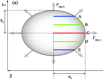
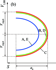
Figure 19: (a) Schematic view of an expanding ellipsoidal shell. (b) Velocity distributions in position ($S$)-velocity diagram.

Figure 19 (a) shows a schematic view of an expanding ellipsoidal shell. Assuming the arc cloud and H I shell are part of an expanding shell, we model the shell to be an ellipsoid with a semimajor axis $a_{0}$ of 45 pc, semiminor axis $b_{0}$ of 32 pc and a 3rd axis in the depth direction which has the same length as the minor axis (prolate spheroid). Figure 19 (b) shows position($S$)-velocity diagrams sliced along the lines of A – E in Figure 19 (a). If the shell is expanding with velocities of $V_{\rm exp,a}:V_{\rm exp,b}=45:32$, an elliptical feature is expected in the position($S$)-velocity diagram as shown in Figure 19 (b). The velocity distribution systematically shifts with the projected radius from the center of the shell as shown by red, green and blue colors. Note that the distributions in Figure 19 (b) are represented only for the western half.

Appendix B EVOLUTION OF SNR

A simple model of the evolution of SNRs is explained by three phases; the free expansion phase in which the shock velocity is constant, the Sedov-Taylor phase in which the shock expands adiabatically, and the radiative phase in which the energy is lost by radiation (e.g., Sturner et al., 1997; Yamazaki et al., 2006). The shock velocity $V_{\rm s}$ for each phase is written by function of the age of SNRs $t$ as follows;

$$V_{\rm s}(t)=\left\{\begin{array}[]{l l l}v_{\rm i}&(0\leq t<t_{1})&\mbox{: Free expansion phase}\\ v_{\rm i}\left(\frac{t}{t_{1}}\right)^{-3/5}&(t_{1}\leq t<t_{2})&\mbox{: Sedov-Taylor phase}\\ v_{\rm i}\left(\frac{t_{2}}{t_{1}}\right)^{-3/5}\left(\frac{t}{t_{2}}\right)^{-2/3}&(t_{2}\leq t)&\mbox{: Radiative phase}\end{array}\right.$$ (B1)

where $v_{\rm i}$ is the initial shock velocity when the supernova explosion occurs. $t_{1}$ and $t_{2}$ are transition time from the free expansion phase and Sedov-Taylor phase, respectively, to the next phases, and are written as $t_{1}=2.1\times 10^{2}E_{51}^{1/3}n_{0}^{-1/3}v_{\rm i,4}^{-5/3}$ yr and $t_{2}=4\times 10^{4}E_{51}^{4/17}n_{0}^{-9/17}$ yr (Blondin et al., 1998). $E_{51}$ is an expansion energy in unit of $10^{51}$ erg, and $n_{0}$ is an uniform ambient density in unit of cm^-3. $v_{\rm i,4}$ is given from $v_{\rm i}=v_{\rm i,4}\times 10^{4}$ km s^-1. For the radiative phase, we use that the evolution of the shock velocity obeys $\propto t^{-2/3}$ approximately in the epoch of 10⁵ yr (Blondin et al., 1998; Bandiera & Petruk, 2004).

Radius of an SNR are derived by integrating (B1) along the time, i.e. $R(t)=\int V_{\rm s}(t)dt$. We show the radii in the free expansion phase $R_{\rm f}$, the Sedov-Taylor phase $R_{\rm s}$, and the radiative phase $R_{\rm f}$ in the follows,

$$R(t)=\left\{\begin{array}[]{ll}R_{\rm f}(t)=v_{\rm i}t&(0\leq t<t_{1})\\ R_{\rm s}(t)=\frac{5}{2}v_{\rm i}\left(t_{1}^{3/5}t^{2/5}-t_{1}\right)+R_{\rm f}(t_{1})&(t_{1}\leq t<t_{2})\\ R_{\rm r}(t)=3v_{\rm i}t_{1}^{3/5}\left(t_{2}^{1/15}t^{1/3}-t_{2}^{2/5}\right)+R_{\rm s}(t_{2})&(t_{2}\leq t)\end{array}\right.$$ (B2)

Mass swept by the SNR $M_{\mathrm{swept}}$ is estimated by

$$M_{\mathrm{swept}}=\frac{4\pi}{3}R(t)^{3}m_{\rm H}n_{0}.$$ (B3)

Table 1: Observed transitions and telescopes

Line	HPBW	Velocity resolution	$T_{\rm rms}$	Telescope	Mode
	(arcsec)	(km s-1)	(K)
12CO($J$=2–1)	100	0.33	0.2	NANTEN2	OTF
13CO($J$=2–1)	100	0.34	0.09	NANTEN2	PSW
12CO($J$=1–0)	47	0.088	1.0	Mopra	OTF
13CO($J$=1–0)	47	0.092	0.4	Mopra	OTF

Table 2: Observed parameters of ¹²CO($J$=2–1) with NANTEN2

Region	Position					Peak properties
	$l$	$b$	$S$	$T$		$T_{\rm MB}$	$V_{\rm LSR}$	$\Delta V$	$W_{\rm CO}$	$\Delta V_{\rm comp}$
	(degree)					(K)	(km s-1)	(km s-1)	(K km s-1)	(km s-1)
Arc	283.97	$-$0.15	$-$0.35	0.02		2.9	26.3	4.8	15.2	2.6
J1	284.32	$-$0.51	0.15	$-$0.03		1.7	29.0	1.9	3.5	2.4
J2	284.64	$-$0.73	0.54	0.00		1.6	28.8	4.4	6.6	4.9
J3	284.94	$-$0.87	0.85	0.09		4.5	26.2	2.4	11.7	4.0
J4	284.60	$-$0.69	0.48	0.00		2.5	22.5	3.7	8.7	3.4
J5	284.83	$-$0.78	0.72	0.08		4.1	21.3	3.5	14.7	3.7

Table 3: Observed parameters of ¹²CO($J$=1–0) with Mopra Telescope

Region	Position					Peak properties
	$l$	$b$	$S$	$T$		$T_{\rm MB}$	$V_{\rm LSR}$	$\Delta V$	$W_{\rm CO}$	$\Delta V_{\rm comp}$
	(degree)					(K)	(km s-1)	(km s-1)	(K km s-1)	(km s-1)
Arc	283.97	$-$0.15	$-$0.36	0.02		6.4	26.4	4.1	26.4	2.5
J1	284.45	$-$0.59	0.30	$-$0.01		4.0	28.7	2.5	10.9	2.3
J2	284.62	$-$0.72	0.52	$-$0.01		3.6	28.8	3.7	13.2	4.8
J3	284.94	$-$0.87	0.85	0.08		13.7	26.2	2.2	32.7	4.1
J4	284.58	$-$0.70	0.47	$-$0.01		6.7	22.9	2.6	18.2	3.6
J5	284.83	$-$0.79	0.72	0.08		9.3	21.2	2.7	26.6	3.7

Table 4: Observed parameters of ¹³CO($J$=1–0) with Mopra Telescope

Region	Position					Peak properties
	$l$	$b$	$S$	$T$		$T_{\rm MB}$	$V_{\rm LSR}$	$\Delta V$	$W_{\rm CO}$	$\Delta V_{\rm comp}$
	(degree)					(K)	(km s-1)	(km s-1)	(K km s-1)	(km s-1)
Arc	283.97	$-$0.15	$-$0.35	0.02		2.4	26.1	2.1	5.4	1.9
J1	284.45	$-$0.57	0.29	0.00		0.8	28.3	1.7	1.8	2.1
J2	284.62	$-$0.73	0.52	$-$0.01		0.3	29.1	2.4	0.8	3.9
J3	284.94	$-$0.86	0.85	0.09		3.3	26.2	1.7	6.2	2.4
J4	284.58	$-$0.69	0.46	$-$0.01		1.7	23.0	1.4	2.5	2.1
J5	284.84	$-$0.79	0.72	0.08		2.5	21.2	2.1	5.7	2.7

Table 5: Physical properties of molecular clouds

Region	peak $N({\rm H_{2}})$	$r$	$M$
	(1021 cm-2)	(pc)	($10^{4}\,M_{\sun}$)
Arc	2.7	18.6	2.5
WJ	1.4	7.2	0.3
J1	1.7	9.9	0.6
J2	2.7	11.6	1.0
J3	4.8	15.9	2.1
J4	2.9	8.2	0.5
J5	4.8	11.7	1.4

Table 6: Observed parameters used in LVG analysis and results of LVG analysis.

Region	Position					Averaged intensities				LVG results
	$l$	$b$	$S$	$T$		$T_{\rm obs1}$	$T_{\rm obs2}$	$T_{\rm obs3}$	$V_{\rm G}$	$n({\rm H}_{2})$	$T_{\rm kin}$
	(degree)					(K)			(km s-1)	(cm-3)	(K)
p	283.97	$-$0.15	$-$0.35	0.02		2.63	1.73	0.91	26.0	$1.4_{-0.1}^{+0.1}\times 10^{3}$	$9_{-2}^{+2}$
q	284.27	$-$0.43	0.06	0.00		1.38	0.48	0.11	29.2	$\leq 5.0\times 10^{2}$	$\leq 6$
r	284.32	$-$0.53	0.16	$-$0.04		1.22	0.35	0.12	29.1	$5.6_{-0.1}^{+0.0}\times 10^{2}$	$9_{-1}^{+1}$
s	284.45	$-$0.58	0.29	$-$0.01		0.89	0.44	0.10	28.6	$\leq 5.9\times 10^{2}$	$\leq 6$
t-1	284.62	$-$0.73	0.51	$-$0.01		1.06	0.25	0.11	24.2	$5.9_{-0.2}^{+0.1}\times 10^{2}$	$13_{-2}^{+2}$
t-2						1.09	0.22	0.10	28.8	$5.6_{-0.2}^{+0.1}\times 10^{2}$	$15_{-3}^{+3}$
u-1	284.77	$-$0.81	0.68	0.02		1.16	0.20	0.11	22.2	$5.9_{-0.3}^{+0.2}\times 10^{2}$	$20_{-5}^{+5}$
u-2						1.90	0.46	0.19	26.2	$5.7_{-0.1}^{+0.2}\times 10^{2}$	$12_{-2}^{+2}$
v	284.75	$-$0.98	0.78	$-$0.13		1.36	0.27	0.16	26.4	$7.2_{-0.3}^{+0.6}\times 10^{2}$	$21_{-5}^{+7}$
w	284.93	$-$0.87	0.85	0.08		4.10	1.55	1.08	26.5	$1.3_{-0.2}^{+0.2}\times 10^{3}$	$16_{-4}^{+6}$

Table 7: AKARI sources

Catalog	ID	Band	Flux density
		(µm)	(Jy)
IRC PSC	1026103-583340	9	$0.313\pm 0.019$
FIS BSC	1026099-583345	160	$17.8\pm 7.6$

References

- Abdo et al. (2009a) Abdo, A. A., Ackermann, M., Ajello, M., et al. 2009a, ApJ, 701, L123
- Abdo et al. (2009b) —. 2009b, ApJ, 706, L56
- Abramowski et al. (2012a) Abramowski, A., Acero, F., Aharonian, F., et al. 2012a, A&A, 537, A114
- Abramowski et al. (2012b) —. 2012b, A&A, 548, A38
- Acciari et al. (2008) Acciari, V. A., Beilicke, M., Blaylock, G., et al. 2008, ApJ, 679, 1427
- Ackermann et al. (2011) Ackermann, M., Ajello, M., Baldini, L., et al. 2011, ApJ, 726, 35
- Aharonian et al. (2005) Aharonian, F., Akhperjanian, A. G., Aye, K.-M., et al. 2005, Science, 307, 1938
- Aharonian et al. (2006a) Aharonian, F., Akhperjanian, A. G., Bazer-Bachi, A. R., et al. 2006a, A&A, 460, 743
- Aharonian et al. (2006b) —. 2006b, A&A, 449, 223
- Aharonian et al. (2006c) —. 2006c, A&A, 460, 365
- Aharonian et al. (2007a) —. 2007a, A&A, 467, 1075
- Aharonian et al. (2007b) —. 2007b, ApJ, 661, 236
- Aharonian et al. (2007c) —. 2007c, A&A, 464, 235
- Aharonian et al. (2009) Aharonian, F., Akhperjanian, A. G., de Almeida, U. B., et al. 2009, ApJ, 692, 1500
- Albert et al. (2006) Albert, J., Aliu, E., Anderhub, H., et al. 2006, Science, 312, 1771
- Albert et al. (2007) —. 2007, ApJ, 665, L51
- Ascenso et al. (2007) Ascenso, J., Alves, J., Beletsky, Y., & Lago, M. T. V. T. 2007, A&A, 466, 137
- Bandiera & Petruk (2004) Bandiera, R., & Petruk, O. 2004, A&A, 419, 419
- Bednarek (2007) Bednarek, W. 2007, MNRAS, 382, 367
- Bell (1978) Bell, A. R. 1978, MNRAS, 182, 147
- Bertsch et al. (1993) Bertsch, D. L., Dame, T. M., Fichtel, C. E., et al. 1993, ApJ, 416, 587
- Blandford & Ostriker (1978) Blandford, R. D., & Ostriker, J. P. 1978, ApJ, 221, L29
- Bloemen et al. (1986) Bloemen, J. B. G. M., Strong, A. W., Mayer-Hasselwander, H. A., et al. 1986, A&A, 154, 25
- Blondin et al. (1998) Blondin, J. M., Wright, E. B., Borkowski, K. J., & Reynolds, S. P. 1998, ApJ, 500, 342
- Blundell & Bowler (2004) Blundell, K. M., & Bowler, M. G. 2004, ApJ, 616, L159
- Bosch-Ramon et al. (2005) Bosch-Ramon, V., Aharonian, F. A., & Paredes, J. M. 2005, A&A, 432, 609
- Brand & Blitz (1993) Brand, J., & Blitz, L. 1993, A&A, 275, 67
- Brinkmann et al. (1996) Brinkmann, W., Aschenbach, B., & Kawai, N. 1996, A&A, 312, 306
- Dame (2007) Dame, T. M. 2007, ApJ, 665, L163
- Dame et al. (2001) Dame, T. M., Hartmann, D., & Thaddeus, P. 2001, ApJ, 547, 792
- Dawson et al. (2011) Dawson, J. R., McClure-Griffiths, N. M., Kawamura, A., et al. 2011, ApJ, 728, 127
- Deharveng et al. (2010) Deharveng, L., Schuller, F., Anderson, L. D., et al. 2010, A&A, 523, A6
- Dubner et al. (1998) Dubner, G. M., Holdaway, M., Goss, W. M., & Mirabel, I. F. 1998, AJ, 116, 1842
- Fermi LAT Collaboration (2009) Fermi LAT Collaboration. 2009, Science, 326, 1512
- Frerking et al. (1982) Frerking, M. A., Langer, W. D., & Wilson, R. W. 1982, ApJ, 262, 590
- Fujita et al. (2009a) Fujita, Y., Hayashida, K., Takahashi, H., & Takahara, F. 2009a, PASJ, 61, 1229
- Fujita et al. (2009b) Fujita, Y., Ohira, Y., Tanaka, S. J., & Takahara, F. 2009b, ApJ, 707, L179
- Fukui et al. (2009) Fukui, Y., Furukawa, N., Dame, T. M., et al. 2009, PASJ, 61, L23
- Furukawa et al. (2009) Furukawa, N., Dawson, J. R., Ohama, A., et al. 2009, ApJ, 696, L115
- Gabici et al. (2009) Gabici, S., Aharonian, F. A., & Casanova, S. 2009, MNRAS, 396, 1629
- Gallo et al. (2005) Gallo, E., Fender, R., Kaiser, C., et al. 2005, Nature, 436, 819
- Goldreich & Kwan (1974) Goldreich, P., & Kwan, J. 1974, ApJ, 189, 441
- Goldsmith & Langer (1978) Goldsmith, P. F., & Langer, W. D. 1978, ApJ, 222, 881
- Grabelsky et al. (1987) Grabelsky, D. A., Cohen, R. S., Bronfman, L., Thaddeus, P., & May, J. 1987, ApJ, 315, 122
- H.E.S.S. Collaboration (2011a) H.E.S.S. Collaboration. 2011a, A&A, 531, A81
- H.E.S.S. Collaboration (2011b) —. 2011b, A&A, 525, A46
- Hjellming & Johnston (1981) Hjellming, R. M., & Johnston, K. J. 1981, ApJ, 246, L141
- Holder et al. (2006) Holder, J., Atkins, R. W., Badran, H. M., et al. 2006, Astroparticle Physics, 25, 391
- Hunter et al. (1997) Hunter, S. D., Bertsch, D. L., Catelli, J. R., et al. 1997, ApJ, 481, 205
- Inoue et al. (2006) Inoue, T., Inutsuka, S.-i., & Koyama, H. 2006, ApJ, 652, 1331
- Kargaltsev & Pavlov (2010) Kargaltsev, O., & Pavlov, G. G. 2010, X-ray Astronomy 2009; Present Status, Multi-Wavelength Approach and Future Perspectives, 1248, 25
- Kataza et al. (2010) Kataza, H., Allfageme, C., Cassatella, N., et al. 2010, AKARI/IRC All-Sky Survey Point Source Catalogue Version 1.0 Release Note, (Kanagawa, Japan: Institute of Space and Astronautical Science)
- Kawada et al. (2007) Kawada, M., Baba, H., Barthel, P. D., et al. 2007, PASJ, 59, 389
- Ladd et al. (2005) Ladd, N., Purcell, C., Wong, T., & Robertson, S. 2005, PASA, 22, 62
- Lorenz (2004) Lorenz, E. 2004, New A Rev., 48, 339
- Manchester et al. (2005) Manchester, R. N., Hobbs, G. B., Teoh, A., & Hobbs, M. 2005, AJ, 129, 1993
- Manolakou et al. (2007) Manolakou, K., Horns, D., & Kirk, J. G. 2007, A&A, 474, 689
- McClure-Griffiths et al. (2005) McClure-Griffiths, N. M., Dickey, J. M., Gaensler, B. M., et al. 2005, ApJS, 158, 178
- Michelson et al. (2010) Michelson, P. F., Atwood, W. B., & Ritz, S. 2010, Reports on Progress in Physics, 73, 074901
- Milam et al. (2005) Milam, S. N., Savage, C., Brewster, M. A., Ziurys, L. M., & Wyckoff, S. 2005, ApJ, 634, 1126
- Mizuno & Fukui (2004) Mizuno, A., & Fukui, Y. 2004, in Astronomical Society of the Pacific Conference Series, Vol. 317, Milky Way Surveys: The Structure and Evolution of our Galaxy, ed. D. Clemens, R. Shah, & T. Brainerd, 59
- Mizuno et al. (1995) Mizuno, A., Onishi, T., Yonekura, Y., et al. 1995, ApJ, 445, L161
- Mizuno et al. (2001) Mizuno, A., Yamaguchi, R., Tachihara, K., et al. 2001, PASJ, 53, 1071
- Mizuno et al. (2010) Mizuno, Y., Kawamura, A., Onishi, T., et al. 2010, PASJ, 62, 51
- Murphy et al. (2007) Murphy, T., Mauch, T., Green, A., et al. 2007, MNRAS, 382, 382
- Nakajima et al. (2007) Nakajima, T., Kaiden, M., Korogi, J., et al. 2007, PASJ, 59, 1005
- Nakamura et al. (2001) Nakamura, M., Uchida, Y., & Hirose, S. 2001, New A, 6, 61
- Obayashi et al. (1998) Obayashi, A., Kun, M., Sato, F., Yonekura, Y., & Fukui, Y. 1998, AJ, 115, 274
- Ohama et al. (2010) Ohama, A., Dawson, J. R., Furukawa, N., et al. 2010, ApJ, 709, 975
- Onaka et al. (2007) Onaka, T., Matsuhara, H., Wada, T., et al. 2007, PASJ, 59, 401
- Paredes et al. (2002) Paredes, J. M., Ribó, M., & Martí, J. 2002, A&A, 394, 193
- Piatti et al. (1998) Piatti, A. E., Bica, E., & Claria, J. J. 1998, A&AS, 127, 423
- Portegies Zwart et al. (2010) Portegies Zwart, S. F., McMillan, S. L. W., & Gieles, M. 2010, ARA&A, 48, 431
- Rauw et al. (2007) Rauw, G., Manfroid, J., Gosset, E., et al. 2007, A&A, 463, 981
- Rauw et al. (2011) Rauw, G., Sana, H., & Nazé, Y. 2011, A&A, 535, A40
- Rauw et al. (2005) Rauw, G., Crowther, P. A., De Becker, M., et al. 2005, A&A, 432, 985
- Reach et al. (1998) Reach, W. T., Wall, W. F., & Odegard, N. 1998, ApJ, 507, 507
- Russell et al. (2007) Russell, D. M., Fender, R. P., Gallo, E., & Kaiser, C. R. 2007, MNRAS, 376, 1341
- Sabatini et al. (2010) Sabatini, S., Tavani, M., Striani, E., et al. 2010, ApJ, 712, L10
- Saz Parkinson et al. (2010) Saz Parkinson, P. M., Dormody, M., Ziegler, M., et al. 2010, ApJ, 725, 571
- Schneider et al. (1998) Schneider, N., Stutzki, J., Winnewisser, G., & Block, D. 1998, A&A, 335, 1049
- Sturner et al. (1997) Sturner, S. J., Skibo, J. G., Dermer, C. D., & Mattox, J. R. 1997, ApJ, 490, 619
- Tavani et al. (2009) Tavani, M., Barbiellini, G., Argan, A., et al. 2009, A&A, 502, 995
- Véron-Cetty & Véron (2010) Véron-Cetty, M.-P., & Véron, P. 2010, A&A, 518, A10
- Whiteoak & Uchida (1997) Whiteoak, J. B. Z., & Uchida, K. I. 1997, A&A, 317, 563
- Yamaguchi et al. (1999) Yamaguchi, R., Saito, H., Mizuno, N., et al. 1999, PASJ, 51, 791
- Yamamoto et al. (2008) Yamamoto, H., Ito, S., Ishigami, S., et al. 2008, PASJ, 60, 715
- Yamamura et al. (2010) Yamamura, I., Makiuti, S., Ikeda, N., et al. 2010, AKARI/FIS All-Sky Survey Bright Source Catalogue Version 1.0 Release Note, (Kanagawa, Japan: Institute of Space and Astronautical Science)
- Yamazaki et al. (2006) Yamazaki, R., Kohri, K., Bamba, A., et al. 2006, MNRAS, 371, 1975
- Zavagno et al. (2006) Zavagno, A., Deharveng, L., Comerón, F., et al. 2006, A&A, 446, 171