The far-zone interatomic Casimir-Polder potential between two ground-state atoms outside a Schwarzschild black hole

Abstract

Based on the idea that the vacuum fluctuations of electromagnetic fields can induce instantaneous correlated dipoles, we study the far-zone Casimir-Polder potential between two atoms in the Boulware, Unruh and Hartle-Hawking vacua outside a Schwarzschild black hole. We show that, at spatial infinity, the Casimir-Polder potential in the Boulware vacuum is similar to that in the Minkowski vacuum in flat spacetime with a behavior of $R^{-7}$, so is in the Unruh vacuum as a result of the backscattering of the Hawking radiation from the black hole off the spacetime curvature. However, the interatomic Casimir-Polder potential in the Hartle-Hawking vacuum behaves like that in a thermal bath at the Hawking temperature. In the region near the event horizon of the black hole, the modifications caused by the space-time curvature make the interatomic Casimir-Polder potential smaller in all three vacuum states.

I Introduction

The Casimir effect which can be considered as one of the macroscopical observable phenomena originating from the vacuum field fluctuations was firstly discussed by Casimir in 1948  Casimir-1 . Casimir predicted that vacuum fluctuations give rise to an attractive force between two neutral conducting plates at rest. In the same year, Casimir and Polder also began the pioneering work on the retarded dispersion interaction between two atoms(or molecules) Casimir-Polder . For atoms having a dominant transition with frequency $\omega_{0}$ between the ground and first excited states, they showed that the interaction between the two atoms reduced to the London limit of the van der Waals interaction in the near zone, i.e., $R^{-6}$ dependence for small separations ($R\omega_{0}\ll 1$). In contrast, the interaction energy decays like $R^{-7}$ in the far zone Casimir-Polder . So far, the Casimir and Casimir-Polder forces have been measured with remarkable precision in experiments Sukenik-ex .

Since space-time geometry and the presence of boundaries can affect vacuum field fluctuations, it is expected that the Casimir-Polder interaction will be modified in these circumstances. In this regard, the Casimir-Polder interaction between two atoms placed near the conducting plate was studied by Spagnolo et al  Spagnolo . A natural question along that line is what happens when the two-atoms system is placed in curved spacetime rather than a flat spacetime. This is what we are going to do in the present paper, i.e., we are going to investigate the Casimir-Polder potential between two neutral but polarizable atoms outside a spherically symmetric black hole. Let us note, as examples of related effects that also arise as a result of the modification of vacuum fluctuations due to the presence of spacetime curvature, that the Lamb shift of a static atom zhy-1 ; zhy-2 and the Casimir-Polder-like force on it zhjl outside a Schwarzschild black hole have recently been studied.

There are numerous methods aimed at obtaining the Casimir-Polder potential, such as those using two-transverse-photon exchange within perturbation theory margenau-book ; Craig-book , consideration of the changes in zero-point energy Boyer , radiative reaction  PMilonni , evaluation of energy shifts in the Heisenberg picture Power , the method based on spatial vacuum field correlationsPower-Thirunamachandran ; Spagnolo , the response theory  Barash-book and so on. A general treatment within a relativistic framework is reviewed by Feinberg and Sucher Feinberg . Our calculation of the interatomic Casimir-Polder potential is based upon the method of equal-time spatial vacuum field correlations which can simplify some calculations in some complex external environment. The main idea based on the vacuum spatial correlations can be narrated as that the vacuum fluctuations of the electromagnetic field induce instantaneous correlated dipole moments on the two atoms and the Casimir-Polder potential energy can be obtained by calculating the classical interaction between the two correlated induced dipoles Power-Thirunamachandran ; Spagnolo .

The paper is organized as follows. In the next section, we will give the basic formula of interatomic Casimir-Polder potential between the two ground-state atoms in the far zone. Then we will calculate Casimir-Polder potential caused by induced instantaneous atomic dipoles generated by electromagnetic field fluctuations in the Boulware vacuum Boulware , Unruh vacuum  Unruh and Hartle-Hawking vacuum  Hartlehawking , In Secs. III, IV, and V respectively. Finally, we will conclude in Sec. VI.

II The field spatial correlation function and the interatomic Casimir-Polder potential

Within the dipole approximation, the Hamiltonian of a system composed of two atoms A and B interacting with external radiation fields in the multipolar scheme can be written as

$$H=H_{F}+H^{A}_{atom}+H^{B}_{atom}-{\bf{\mu}}_{A}\cdot{\bf{D}}({\bf{r}}_{A})-{\bf{\mu}}_{B}\cdot{\bf{D}}({\bf{r}}_{B})\;,$$ (1)

where ${\bf{D}}({\bf{r}}_{A})=\sum{\bf{D}}(\omega_{\bf{k}},{\bf{r}}_{A})$ denotes the transverse displacement electric field operator at the point ${\bf{r}}_{A}$ and ${\bf{\mu}}_{A}$ (or ${\bf{\mu}}_{B}$) indicates the electric dipole operator of atom A ( or B). For the two atoms which are fixed at the certain locations in a space-time, the vacuum fluctuations of the electromagnetic field induce instantaneous correlated dipole moments on them as a result of the spatially correlated vacuum fluctuations. The Casimir-Polder potential energy then can be considered as the (classical) interaction between the two correlated induced dipoles. The induced dipole moments caused by the vacuum fluctuations usually can be written as Power-Thirunamachandran ; Spagnolo : $\mu_{l}(\omega_{\bf{k}})=\alpha(\omega_{\bf{k}})D_{l}(\omega_{\bf{k}},{\bf{r}})\;,$ where

$$\alpha(\omega_{\bf{k}})=\frac{2}{3}\sum_{m}\frac{E_{m0}\mu_{m0}^{2}}{E_{m0}^{2}-\omega_{\bf{k}}^{2}}$$ (2)

is the atomic dynamical isotropic polarizability (here $E_{m0}=E_{m}-E_{0}$ and $\mu_{m0}$ denote the matrix elements of the atomic dipole moment operator). For the case of a two-level atom, the isotropic polarizability can be written as

$$\alpha(\omega_{\bf{k}})=\frac{2\omega_{0}\mu^{2}}{3(\omega_{0}^{2}-\omega_{\bf{k}}^{2})}\;.$$ (3)

Therefore, the interatomic Casimir-Polder potential of two ground-state atoms reads  Power-Thirunamachandran ; Spagnolo

$$V_{AB}=\int\sum_{ij}\alpha_{A}(\omega_{\bf{k}})\alpha_{B}(\omega_{\bf{k}})\langle{D_{i}(\omega_{\bf{k}},{\bf{r_{A}}})}{D_{j}(\omega_{\bf{k}},{\bf{r_{B}}})}\rangle{V}_{ij}(\omega_{\bf{k}},R)d\omega_{\bf{k}}\;,$$ (4)

where $\langle{D_{i}(\omega_{\bf{k}},{\bf{r_{A}}})}{D_{j}(\omega_{\bf{k}},{\bf{r_{B}}})}\rangle$ is the equal-time spatial correlation function of the electric field in the vacuum state and ${V}_{ij}(\omega_{\bf{k}},R)$ is the classical electrostatic interaction energy between two dipoles oscillating at frequency $\omega_{\bf{k}}$ McLone

$${V}_{ij}(\omega_{\bf{k}},R)=(\delta_{ij}-3\hat{R_{i}}\hat{R_{j}})\bigg{[}\frac{\cos(\omega_{\bf{k}}R)}{R^{3}}+\frac{\omega_{\bf{k}}\sin(\omega_{\bf{k}}R)}{R^{2}}\bigg{]}-(\delta_{ij}-\hat{R_{i}}\hat{R_{j}})\frac{\omega^{2}_{\bf k}\cos(\omega_{\bf{k}}R)}{R}\;,$$ (5)

where the distance of the two atoms is denoted by $R=|\bf{r_{A}}-\bf{r_{B}}|$ and $\hat{R_{i}}={R_{i}}/R$ denotes the $i$-th element of the unit displacement vector of ${\bf{R}}/R\;$. In the far zone ($R\omega_{0}\gg 1$), the retardation effect becomes significant, and we can replace the dynamical polarizabilities $\alpha_{A,B}(\omega_{\bf{k}})$ with their static polarizabilities $\alpha_{A,B}(\omega_{\bf{k}})\simeq\alpha_{A,B}(0)\;$ Spagnolo ; Milonni . Then we can write Eq. (4) in the far zone as

$$V_{AB}=\alpha_{A}(0)\alpha_{B}(0)\int\sum_{ij}\langle{D_{i}(\omega_{\bf{k}},{\bf{r_{A}}})}{D_{j}(\omega_{\bf{k}},{\bf{r_{B}}})}\rangle{V}_{ij}(\omega_{\bf{k}},R)d\omega_{\bf{k}}\;.$$ (6)

For a Schwarzschild black hole, there are three vacuum states which can be defined by the nonoccupation of positive frequency modes, i.e., the Boulware, Hartle-Hawking and Unruh vacua. In the following, we will examine in detail Eq. (6) in these vacuum states outside a Schwarzschild black hole.

III the interatomic Casimir-Polder potential in Boulware vacuum

Consider the two atoms in interaction with vacuum electromagnetic fluctuations outside a four-dimensional spherically symmetric black hole. The line element of the space-time is given by

$$ds^{2}=g_{\mu\nu}dx^{\mu}dx^{\nu}=(1-2M/r)dt^{2}-(1-2M/r)^{-1}dr^{2}-r^{2}(d\theta^{2}+\sin^{2}\theta{d\phi^{2}})\;,$$ (7)

where M is the mass of the black hole. Now we suppose that the field is in a vacuum state, and for simplicity, the two atoms are fixed along the same radial direction(see Fig. (1 )). Then we do not need to calculate the contributions of spatial field correlation function in $\theta-$ and $\phi-$directions. In this case, Eq. (6) can be simplified as

$$V_{AB}=\alpha_{A}(0)\alpha_{B}(0)\int\langle{D_{r}(\omega_{\bf{k}},r_{A})}{D_{r}(\omega_{\bf{k}},r_{B})}\rangle{V}_{rr}(\omega_{\bf{k}},R)d\omega_{\bf{k}}\;,$$ (8)

with

$${V}_{rr}(\omega_{\bf{k}},R)=-2\bigg{[}\frac{\cos(\omega_{\bf{k}}R)}{R^{3}}+\frac{\omega_{\bf{k}}\sin(\omega_{\bf{k}}R)}{R^{2}}\bigg{]}\;.$$ (9)

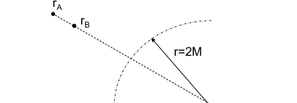
Figure 1: The dashed arc denotes the event horizon of a black hole. Suppose that atom A and atom B are fixed along the same radial direction, then $R=r_{A}-r_{B}\;.$

For the case of the Boulware vacuum, the two point function has been given in Ref. ZhouYu-1

$$\langle{D}_{r}(x_{A}){D}_{r}(x_{B})\rangle = \frac{1}{4\pi}\sum_{l}\int_{0}^{\infty}d\omega\;\omega\;e^{-i\omega(t-t^{\prime})}(2l+1)\;$$ (10)

$$\quad\;\quad\;\;\times[\overrightarrow{R}_{l}(\omega|r_{A})\overrightarrow{R}^{\star}_{l}(\omega|r_{B})+\overleftarrow{R}_{l}(\omega|r_{A})\overleftarrow{R}^{\star}_{l}(\omega|r_{B})]\;,$$

where $\overrightarrow{R}_{l}$ and $\overleftarrow{R}_{l}$ represent the auxiliary radial function of the outgoing modes from the past horizon $H^{-}$ and the incoming modes from the past null infinity $\mathcal{J}^{-}$ respectively Luis . Here, the constant coefficient is different from that given in Ref. ZhouYu-1 because of the different unit systems. Besides these, it should be pointed out that $\omega$ in Eq. (10) is concerned with the coordinate time $t$. However, for the atom fixed at a point of a static space-time, the proper frequency $\omega_{\bf{k}}$ should be associated with the proper time $\tau$ in the local inertial frame of the atom. For the case of $r_{A},r_{B}\rightarrow\infty$, it is easy to obtain that $g_{00}^{A}\simeq g_{00}^{B}=g_{00}\sim 1\;.$ When two atoms are fixed near the event horizon, we will assume that the distance of the system from the event horizon is much larger than the size of the two-atom system itself, i.e., $R/L\ll 1,\;{L}/(2M)\ll 1$ with $L=r_{B}-2M$, then $g_{00}^{A}\simeq g_{00}^{B}=g_{00}\;$. Consequently, the equal-time (proper time $\tau$) correlation function can be obtained by using the relation of $\omega=\sqrt{g_{00}}\omega_{\bf{k}}$, since our discussions will be focused on two asymptotic regions, i.e, at the spatial infinity and near the event horizon. So, we have

$$\langle{D_{r}(\omega_{\bf{k}},r_{A})}{D_{r}(\omega_{\bf{k}},r_{B})}\rangle= \frac{g_{00}}{4\pi}\sum_{l}{\omega_{\bf{k}}}(2l+1)\big{[}\overrightarrow{R}_{l}(\omega_{\bf{k}}\sqrt{g_{00}}|r_{A})\overrightarrow{R}^{\star}_{l}(\omega_{\bf{k}}\sqrt{g_{00}}|r_{B})$$ (11)

$$+\overleftarrow{R}_{l}(\omega_{\bf{k}}\sqrt{g_{00}}|r_{A})\overleftarrow{R}^{\star}_{l}(\omega_{\bf{k}}\sqrt{g_{00}}|r_{B})]\;.$$

Then Eq. (8) can be evaluated by using the corresponding correlation function

$$V_{AB}= \frac{g_{00}\alpha_{A}(0)\alpha_{B}(0)}{4\pi}\int_{0}^{\infty}\sum_{l}{\omega_{\bf{k}}}(2l+1)\big{[}\overrightarrow{R}_{l}(\omega_{\bf{k}}\sqrt{g_{00}}|r_{A})\overrightarrow{R}^{\star}_{l}(\omega_{\bf{k}}\sqrt{g_{00}}|r_{B})$$ (12)

$$+\overleftarrow{R}_{l}(\omega_{\bf{k}}\sqrt{g_{00}}|r_{A})\overleftarrow{R}^{\star}_{l}(\omega_{\bf{k}}\sqrt{g_{00}}|r_{B})\big{]}\times{V}_{rr}(\omega_{\bf{k}},R)d\omega_{\bf{k}}\;.$$

It is a formidable task to give the exact forms of the auxiliary radial functions. However, the summation concerned with the radial functions in the two asymptotic regions behaves as (see Appendix)

$$\sum_{l}(2l+1)\;\overleftarrow{R}_{l}(p|r_{A})\overleftarrow{R}^{\star}_{l}(p|r_{B})\sim\left\{\begin{array}[]{ll}\frac{\sum_{l}l(l+1)(2l+1)\;|\mathcal{T}_{l}(p)|^{2}}{(2M)^{4}\;p^{2}}e^{-ip\Delta{r_{*}}},&r_{A},r_{B}\sim 2M\;,\\ \frac{8\sin(pR/\sqrt{g_{00}})}{\sqrt{g_{00}}R^{3}p}-\frac{8\cos(pR/\sqrt{g_{00}})}{R^{2}g_{00}}\;,&r_{A},r_{B}\rightarrow\infty\;,\end{array}\right.$$ (13)

and

$$\sum_{l}(2l+1)\;\overrightarrow{R}_{l}(p|r_{A})\overrightarrow{R}^{\star}_{l}(p|r_{B})\sim\left\{\begin{array}[]{ll}\big{(}8p^{2}+\frac{1}{2M^{2}}\big{)}\big{[}\frac{\sin(p{R}/\sqrt{g_{00}})}{\sqrt{g_{00}}p^{3}R^{3}}-\frac{\cos(p{R}/\sqrt{g_{00}})}{g_{00}p^{2}R^{2}}\big{]}\;,&r_{A},r_{B}\sim 2M\;,\\ \frac{\sum_{l}l(l+1)(2l+1)\;|\mathcal{T}_{l}(p)|^{2}}{{p}^{2}r_{A}^{2}r_{B}^{2}}e^{ip\Delta{r_{*}}}\;,&r_{A},r_{B}\rightarrow\infty\;,\end{array}\right.$$ (14)

where $R=r_{A}-r_{B}\;$ and $\Delta{r_{*}}=r_{*}^{A}-r_{*}^{B}$, with the Regge-Wheeler tortoise coordinate defined by $r_{*}=r+2M\ln(r/2M-1).$ For the sake of convenience, we divide the Casimir-Polder potential into two parts: $V_{AB}={\overrightarrow{V}}_{AB}+{\overleftarrow{V}}_{AB}\;,$ where the contribution of the outgoing modes is denoted by

$${\overrightarrow{V}}_{AB}=\frac{g_{00}\alpha_{A}(0)\alpha_{B}(0)}{4\pi}\sum_{l}\int_{0}^{\infty}{\omega_{\bf{k}}}(2l+1)\overrightarrow{R}_{l}(\omega_{\bf{k}}\sqrt{g_{00}}|r_{A})\overrightarrow{R}^{\star}_{l}(\omega_{\bf{k}}\sqrt{g_{00}}|r_{B}){V}_{rr}(\omega_{\bf{k}},R)d\omega_{\bf{k}}\;,$$ (15)

and that of the incoming modes by

$${\overleftarrow{V}}_{AB}=\frac{g_{00}\alpha_{A}(0)\alpha_{B}(0)}{4\pi}\sum_{l}\int_{0}^{\infty}{\omega_{\bf{k}}}(2l+1)\overleftarrow{R}_{l}(\omega_{\bf{k}}\sqrt{g_{00}}|r_{A})\overleftarrow{R}^{\star}_{l}(\omega_{\bf{k}}\sqrt{g_{00}}|r_{B}){V}_{rr}(\omega_{\bf{k}},R)d\omega_{\bf{k}}\;.$$ (16)

Using Eq. (13) and Eq. (14), we can show that ${\overleftarrow{V}}_{AB}$ can be approximated at spatial infinity as

$${\overleftarrow{V}}_{AB}\simeq-\frac{5\alpha_{A}(0)\alpha_{B}(0)}{2\pi}\frac{1}{R^{7}}\;,$$ (17)

whereas,

$${\overrightarrow{V}}_{AB}\simeq\frac{\alpha_{A}(0)\alpha_{B}(0)}{4\pi}Re\big{[}\int_{0}^{\infty}f(\omega_{\bf{k}},r_{A},r_{B}){V}_{rr}(\omega_{\bf{k}},R)e^{i\omega_{\bf{k}}{R}\sqrt{g_{00}}}\omega_{\bf{k}}^{3}d\omega_{\bf{k}}\big{]}\;,$$ (18)

in which

$$f(\omega_{\bf{k}},r_{A},r_{B})=\frac{\sum_{l}l(l+1)(2l+1)\;|\mathcal{T}_{l}(\omega_{\bf{k}}\sqrt{g_{00}})|^{2}}{\omega_{\bf{k}}^{4}r_{A}^{2}r_{B}^{2}}\$$ (19)

is a grey-body factor that characterizes the backscattering of the electromagnetic field modes off the space-time curvature ZhouYu-1 . This grey-body factor is dependent on the transmission coefficients $|\mathcal{T}_{l}(\omega_{\bf{k}}\sqrt{g_{00}})|^{2}\;$ defined in Ref. ZhouYu-1 , of which the exact analytic expression is not easy to obtain. However, one can show that by using geometrical optics approximation and quantum tunneling, the transmission coefficients can be approximated as Fabbri ; dewitt

$$|\mathcal{T}_{l}(\omega_{\bf{k}}\sqrt{g_{00}})|^{2}\sim\left\{\begin{array}[]{ll}\theta(\sqrt{27}M\omega_{\bf{k}}\sqrt{g_{00}}-l),&M\omega_{\bf{k}}\gg 1\;,\\ 4\big{[}\frac{(l+1)!(l-1)!}{(2l)!(2l+1)!!}\big{]}^{2}(2M\omega_{\bf{k}}\sqrt{g_{00}})^{2l+2}\;,&M\omega_{\bf{k}}\ll 1\;,\end{array}\right.$$ (20)

where $\theta(x)$ represents the Heaviside $\theta$ function. Therefore, the grey-body factor may be approximately written as $f(\omega_{\bf{k}},r_{A},r_{B})\propto 8g_{00}^{2}M^{4}/(3r_{A}^{2}r_{B}^{2})\;.$ As a result, ${\overrightarrow{V}}_{AB}\sim 0$ at spatial infinity.

However, when the two atoms are fixed near the event horizon , the leading terms from the contribution of the outgoing modes become

$${\overrightarrow{V}}_{AB}\simeq-\frac{5\alpha_{A}(0)\alpha_{B}(0)}{2\pi}\frac{1}{R^{7}}-\frac{3\alpha_{A}(0)\alpha_{B}(0)}{16{\pi}M^{2}g_{00}}\frac{1}{R^{5}}\;.$$ (21)

Let us note here that $M^{2}g_{00}\gg{R^{2}}$ since we assume $R/L\ll 1,{L}/(2M)\ll 1$. If the size of the two-atom system is not negligible as compared with its distance from the event horizon(i.e., $R/L\ll 1\;$ is not satisfied), then we can not take $g_{00}^{B}\simeq{g_{00}^{A}}$. Physically, this means that the classical potential tensor of the induced dipoles Eq. (5) can not be established because of the oscillations of the two induced dipoles at significantly different proper frequencies. We can also show that the contribution from the incoming modes behaves as

$${\overleftarrow{V}}_{AB}\simeq\frac{\alpha_{A}(0)\alpha_{B}(0)}{4\pi}Re\big{[}\int_{0}^{\infty}{f(\omega_{\bf{k}},r_{A},r_{B})}{V}_{rr}(\omega_{\bf{k}},R)e^{-i\omega_{\bf{k}}R\sqrt{g_{00}}}\omega_{\bf{k}}^{3}d\omega_{\bf{k}}\big{]}\;,$$ (22)

which is much smaller than Eq. (21) as a result of the vanishingly-small grey-body factor near the even horizon. In summary, the interatomic Casimir-Polder potential in the Boulware vacuum is given by

$$V_{AB}\simeq\left\{\begin{array}[]{ll}-\frac{5\alpha_{A}(0)\alpha_{B}(0)}{2\pi}\frac{1}{R^{7}}\;,&r_{A},r_{B}\rightarrow\infty\;,\\ -\frac{5\alpha_{A}(0)\alpha_{B}(0)}{2\pi}\frac{1}{R^{7}}-\frac{3\alpha_{A}(0)\alpha_{B}(0)}{16{\pi}M^{2}g_{00}}\frac{1}{R^{5}}\;,&r_{A},r_{B}\sim 2M\;.\end{array}\right.$$ (23)

IV the interatomic Casimir-Polder potential in Hartle-Hawking vacuum

For the case of the Hartle-Hawking vacuum, Eq. (8) can also be written as

$$V_{AB} = \frac{g_{00}\alpha_{A}(0)\alpha_{B}(0)}{4\pi}\int_{-\infty}^{\infty}\sum_{l}{\omega_{\bf{k}}}(2l+1)\bigg{[}\frac{\overrightarrow{R}_{l}(\omega_{\bf{k}}\sqrt{g_{00}}|r_{A})\overrightarrow{R}^{\star}_{l}(\omega_{\bf{k}}\sqrt{g_{00}}|r_{B})}{1-e^{-\omega_{\bf{k}}/T}}$$ (24)

$$+\frac{\overleftarrow{R}^{\star}_{l}(\omega_{\bf{k}}\sqrt{g_{00}}|r_{A})\overleftarrow{R}_{l}(\omega_{\bf{k}}\sqrt{g_{00}}|r_{B})}{e^{\omega_{\bf{k}}/T}-1}\bigg{]}\times{V}_{rr}(\omega_{\bf{k}},R)d\omega_{\bf{k}}\;,$$

where $T=T_{H}/\sqrt{g_{00}}$ with $T_{H}=1/(8\pi{M})$ being the usual Hawking temperature  ZhouYu-1 . With the help of the approximate forms of the radial functions in the two asymptotic regions, Eq. (24) can be evaluated, in the case of $r_{A},{r_{B}}\rightarrow\infty$ , to get

$${\overleftarrow{V}}_{AB}\simeq-\frac{4\pi^{2}{T^{3}}\alpha_{A}(0)\alpha_{B}(0)\coth(2\pi{R}T)}{R^{4}\sinh^{2}(2\pi{R}T)}-\frac{4{\pi}T^{2}\alpha_{A}(0)\alpha_{B}(0)}{{R^{5}}\sinh^{2}(2{R}T)}-\frac{2T\alpha_{A}(0)\alpha_{B}(0)\coth(2\pi{R}T)}{{R^{6}}}\;,$$ (25)

and

$${\overrightarrow{V}}_{AB}\simeq\frac{\alpha_{A}(0)\alpha_{B}(0)}{4\pi}Re\big{[}\int_{-\infty}^{\infty}\frac{f(\omega_{\bf{k}},r_{A},r_{B})}{1-e^{-\omega_{\bf{k}}/T}}{V}_{rr}(\omega_{\bf{k}},R)e^{i\omega_{\bf{k}}R\sqrt{g_{00}}}\omega_{\bf{k}}^{3}d\omega_{\bf{k}}\big{]}\;.$$ (26)

At spatial infinity ($r_{A},{r_{B}}\rightarrow\infty$), ${\overleftarrow{V}}_{AB}$ is the dominant term compared with${\overrightarrow{V}}_{AB}\sim{r_{A}^{-2}r_{B}^{-2}}\;.$ Therefore, the interatomic Casimir-Polder potential can be simplified further by only considering ${\overleftarrow{V}}_{AB}$

$$V_{AB}\simeq\left\{\begin{array}[]{ll}-\frac{5\alpha_{A}(0)\alpha_{B}(0)}{2\pi}\frac{1}{R^{7}}-\frac{8\pi^{3}\alpha_{A}(0)\alpha_{B}(0)}{45}\frac{T_{H}^{4}}{R^{3}}\;,&T_{H}R\ll 1\;,\\ -\frac{2T_{H}\alpha_{A}(0)\alpha_{B}(0)}{R^{6}},&T_{H}R\gg 1\;,\end{array}\right.$$ (27)

where $T\sim{T_{H}}$ is taken at spatial infinity. It is obvious to see that $V_{AB}$ is similar to the Casimir-Polder potential at finite temperature  Goedecke ; Spagnolo-2 ; Boyer-2 . This result is consistent with our usual understanding that the Hartle-Hawking vacuum describes a black hole in equilibrium with an infinite sea of black-body radiation at Hawking temperature. When comparing Eq. (26) with Eq. (18), we find out that Eq. (26) is dependant on the temperature $T\;$. This is in accordance with the common belief that thermal flux emanates from the black hole which is partly depleted by backscattering off the space-time curvature on its way to infinity.

In the region near the event horizon of a black hole (i.e., $R/L\ll 1,{L}/(2M)\ll 1\;$), the contribution from the incoming modes behaves as

$${\overleftarrow{V}}_{AB}\simeq\frac{\alpha_{A}(0)\alpha_{B}(0)}{4\pi}Re\big{[}\int_{-\infty}^{\infty}\frac{f(\omega_{\bf{k}},r_{A},r_{B})}{e^{\omega_{\bf{k}}/T}-1}{V}_{rr}(\omega_{\bf{k}},R)e^{i\omega_{\bf{k}}R\sqrt{g_{00}}}\omega_{\bf{k}}^{3}d\omega_{\bf{k}}\big{]}\;.$$ (28)

Obviously, ${\overleftarrow{V}}_{AB}$ is vanishingly small due to the grey-body factor. Then the interatomic Casimir-Polder potential is mainly determined by ${\overrightarrow{V}}_{AB}\;.$ When $R/L\ll 1,{L}/(2M)\ll 1\;$, it is easy to deduce that $TR\ll 1\;.$ Then we find

$$V_{AB}\simeq-\frac{5\alpha_{A}(0)\alpha_{B}(0)}{2\pi}\frac{1}{R^{7}}-\frac{3\alpha_{A}(0)\alpha_{B}(0)}{16{\pi}M^{2}g_{00}}\frac{1}{R^{5}}-\frac{\pi\alpha_{A}(0)\alpha_{B}(0)}{36M^{2}g_{00}}\frac{T^{2}}{R^{3}}-\frac{8\pi^{3}\alpha_{A}(0)\alpha_{B}(0)}{45}\frac{T^{4}}{R^{3}}\;.$$ (29)

According to Eq. (29), it is easy to see that both the curvature of space-time and the thermal radiation make the interatomic Casimir-Polder potential smaller. One can also see that the first two terms Eq. (29) are just the interatomic Casimir-Polder potential near the horizon in the Boulware vacuum (Eq. (23)) and the last two terms can be considered as the contribution of the Hawking radiation of the black hole.

V the interatomic Casimir-Polder potential in Unruh vacuum

For the case of Unruh vacuum, the far-zone interatomic Casimir-Polder potential of two ground-state atoms becomes ZhouYu-1

$$V_{AB} = \frac{g_{00}\alpha_{A}(0)\alpha_{B}(0)}{4\pi}\int_{-\infty}^{\infty}\sum_{l}{\omega_{\bf{k}}}(2l+1)\big{[}\frac{\overrightarrow{R}_{l}(\omega_{\bf{k}}\sqrt{g_{00}}|r_{A})\overrightarrow{R}^{\star}_{l}(\omega_{\bf{k}}\sqrt{g_{00}}|r_{B})}{1-e^{-\omega_{\bf{k}}/T}}$$ (30)

$$+\theta(\omega_{\bf{k}}){\overleftarrow{R}_{l}(\omega_{\bf{k}}\sqrt{g_{00}}|r_{A})\overleftarrow{R}^{\star}_{l}(\omega_{\bf{k}}\sqrt{g_{00}}|r_{B})}\big{]}\times{V}_{rr}(\omega_{\bf{k}},R)d\omega_{\bf{k}}\;.$$

Similarly, we can also obtain the approximate results in the two asymptotic regions. When two atoms are fixed at spatial infinity, the contribution of the outgoing modes is the same as Eq. (26), which is negligible, and then the corresponding Casimir-Polder interatomic potential is mainly determined by the contribution from the incoming modes (similar to Eq. (17))

$$V_{AB}\simeq-\frac{5\alpha_{A}(0)\alpha_{B}(0)}{2\pi}\frac{1}{R^{7}}\;.$$ (31)

When two atoms are fixed near the horizon, the contribution from the incoming modes which reads

$${\overleftarrow{V}}_{AB}\simeq\frac{\alpha_{A}(0)\alpha_{B}(0)}{4\pi}Re[\int_{0}^{\infty}f(\omega_{\bf{k}},r_{A},r_{B}){V}_{rr}(\omega_{\bf{k}},R)e^{-i\omega_{\bf{k}}R\sqrt{g_{00}}}\omega_{\bf{k}}^{3}d\omega_{\bf{k}}\big{]}\;,$$ (32)

is the vanishingly small and the dominant term of the interatomic Casimir-Polder potential arises from the contribution of the outgoing modes. This situation is similar to the case of the Hartle-Hawking vacuum. We then have

$$V_{AB}\simeq-\frac{5\alpha_{A}(0)\alpha_{B}(0)}{2\pi}\frac{1}{R^{7}}-\frac{3\alpha_{A}(0)\alpha_{B}(0)}{16{\pi}M^{2}g_{00}}\frac{1}{R^{5}}-\frac{\pi\alpha_{A}(0)\alpha_{B}(0)}{36M^{2}g_{00}}\frac{T^{2}}{R^{3}}-\frac{8\pi^{3}\alpha_{A}(0)\alpha_{B}(0)}{45}\frac{T^{4}}{R^{3}}\;.$$ (33)

Therefore, we conclude that at spatial infinity the interatomic Casimir-Polder potential in the Unruh vacuum is the same as that in the Boulware vacuum with a $R^{-7}$ behavior and the contribution of the outgoing thermal radiation is negligible as a result of the backscattering off the spacetime on its way to infinity. When the two atoms are fixed near the horizon, the corresponding far-zone interatomic Casimir-Polder potential is the same as that in the Hartle-Hawking vacuum.

VI Conclusion

In this paper, we have studied the far-zone interatomic Casimir-Polder potential between two atoms outside a Schwarzschild black hole. We find that at spatial infinity, the behavior of the Casimir-Polder potential in the Boulware vacuum is similar to that in vacuum in a flat spacetime with a $R^{-7}$ behavior, and the same is true for the Casimir-Polder potential in the Unruh vacuum as a result of the backscattering of the Hawking radiation from the black hole off the spacetime curvature. However, the Casimir-Polder potential in Hartle-Hawking vacuum behaves like that in a thermal bath at the Hawking temperature. Close to the event horizon, the space-time curvature induces modifications to the interatomic Casimir-Polder potential in all three vacuum states, making the potential smaller.

*

Appendix A the summation concerning the radial functions

In order to prove Eq. (13) and Eq. (14), we first introduce some conclusions in Ref. ZhouYu-1 . In the Boulware vacuum, the two point correlation function of electromagnetic fields reads

$$\langle{D}_{r}(x_{A}){D}_{r}(x_{B})\rangle = \frac{g_{00}}{4\pi}\int_{0}^{\infty}d\omega_{\bf{k}}\;\omega_{\bf{k}}\;e^{-i\omega_{\bf{k}}\Delta\tau}\sum_{l}(2l+1)[\overrightarrow{R}_{l}(\omega_{\bf{k}}\sqrt{g_{00}}|r_{A})\overrightarrow{R}^{\star}_{l}(\omega_{\bf{k}}\sqrt{g_{00}}|r_{B})$$ (34)

$$+\overleftarrow{R}_{l}(\omega_{\bf{k}}\sqrt{g_{00}}|r_{A})\overleftarrow{R}^{\star}_{l}(\omega_{\bf{k}}\sqrt{g_{00}}|r_{B})]\;,$$

with

$$R^{(n)}_{l}(\omega|r)=\frac{\sqrt{l(l+1)}}{\omega}\frac{\varphi^{(n)}_{\omega l}(r)}{r^{2}}\;.$$ (35)

Here the label $``n"$ distinguishes between incoming modes (denoted with $n=\leftarrow$) and outgoing modes(denoted with $n=\rightarrow$). The asymptotic expressions of the radial function in the two asymptotic regions single out

$$\overrightarrow{\varphi}_{\omega l}(r)\sim\left\{\begin{array}[]{ll}e^{i\omega r_{*}}+\overrightarrow{\mathcal{R}_{l}}(\omega)\;e^{-i\omega r_{*}}\;,\quad\;\quad\;r\sim 2M\;,\\ \overrightarrow{\mathcal{T}_{l}}(\omega)\;e^{i\omega r_{*}},\quad\;\quad\;\quad\;\quad\;\quad\;\;r\rightarrow\infty\;,\end{array}\right.$$ (38)

$$\overleftarrow{\varphi}_{\omega l}(r)\sim\left\{\begin{array}[]{ll}\overleftarrow{\mathcal{T}_{l}}(\omega)\;e^{-i\omega r_{*}}\;,\quad\;\quad\;\quad\;\quad\quad r\sim 2M\;,\\ e^{-i\omega r_{*}}+\overleftarrow{\mathcal{R}_{l}}(\omega)\;e^{i\omega r_{*}}\;,\quad\;\quad\;r\rightarrow\infty\;.\end{array}\right.$$ (41)

Here $\mathcal{R}$ and $\mathcal{T}$ are, respectively, the reflection and transmission coefficients. If $r_{A}=r_{B}$, it has been proven that (see Appendix in Ref. ZhouYu-1 )

$$\sum_{l}(2l+1)\;|\overleftarrow{R}_{l}(p|r_{B})|^{2}\sim\left\{\begin{array}[]{ll}\frac{\sum_{l}l(l+1)(2l+1)\;|\mathcal{T}_{l}(p)|^{2}}{(2M)^{4}\;p^{2}},\;\quad\;\quad\;r_{A}=r_{B}\sim 2M\;,\\ \frac{8p^{2}}{3g_{00}^{2}}\;,\quad\;\quad\;\quad\;\quad\;\quad\;\quad\;\;\;\;\;\;r_{A}=r_{B}\rightarrow\infty\;,\end{array}\right.$$ (42)

and

$$\sum_{l}(2l+1)\;|\overrightarrow{R}_{l}(p|r_{B})|^{2}\sim\left\{\begin{array}[]{ll}\frac{8p^{2}}{3g_{00}^{2}}+\frac{1}{6M^{2}g_{00}^{2}}\;,\quad\;\quad\;\quad\quad\;r_{A}=r_{B}\sim 2M\;,\\ \frac{\sum_{l}l(l+1)(2l+1)\;|\mathcal{T}_{l}(p)|^{2}}{p^{2}r_{B}^{4}}\;,\quad\;\quad\;r_{A}=r_{B}\rightarrow\infty\;.\end{array}\right.$$ (43)

At spatial infinity ($r_{A},{r_{B}}\rightarrow\infty$), the equal-time correlation function Eq. (34) should be identified with the equal-time correlation function in Minkowski space Power-Thirunamachandran

$$\langle 0|{D}_{i}(x_{A}){D}_{j}(x_{B})|0\rangle=\frac{1}{\pi}\int_{0}^{\infty}d\omega_{\bf{k}}\omega_{\bf{k}}^{3}e^{-i\omega_{\bf{k}}\Delta\tau}\bigg{\{}(\delta_{ij}-\hat{R_{i}}\hat{R_{j}})\frac{\sin(\omega_{\bf{k}}R)}{\omega_{\bf{k}}R}$$

$$+(\delta_{ij}-3\hat{R_{i}}\hat{R_{j}})\bigg{[}\frac{\cos(\omega_{\bf{k}}R)}{\omega_{\bf{k}}^{2}R^{2}}-\frac{\sin(\omega_{\bf{k}}R)}{\omega_{\bf{k}}^{3}R^{3}}\bigg{]}\bigg{\}}\;.$$ (44)

When comparing Eq. (34) with Eq. (A), we obtain that

$$\sum_{l}(2l+1)\overleftarrow{R}_{l}(\omega_{\bf{k}}\sqrt{g_{00}}|r_{A})\overleftarrow{R}^{\star}_{l}(\omega_{\bf{k}}\sqrt{g_{00}}|r_{B})\simeq\frac{8\omega_{\bf{k}}^{2}}{g_{00}}\bigg{[}\frac{\sin(\omega_{\bf{k}}R)}{\omega_{\bf{k}}^{3}R^{3}}-\frac{\cos(\omega_{\bf{k}}R)}{\omega_{\bf{k}}^{2}R^{2}}\bigg{]}\;,$$ (45)

where the term about $\overrightarrow{R}_{l}(\omega_{\bf{k}})$ in Eq. (34) is neglected because this is very small at the asymptotic region due to outgoing modes backscattered off the space-time curvature on their way. Through a simple calculations, we can write Eq. (45) as

$$\sum_{l}(2l+1)\overleftarrow{R}_{l}(p|r_{A})\overleftarrow{R}^{\star}_{l}(p|r_{B}) \simeq \frac{8p^{2}}{3g_{00}^{2}}\bigg{[}\frac{3\sin(p{R}/\sqrt{g_{00}})}{p^{3}R^{3}/\sqrt{g_{00}^{3}}}-\frac{3\cos(p{R}/\sqrt{g_{00}})}{p^{2}R^{2}/g_{00}}\bigg{]}\;.$$ (46)

This agrees with approximative summation relations Eq. (13) in the case of $r_{A},r_{B}\rightarrow\infty$. For the case $r_{A},r_{B}\sim 2M$, the corresponding result is easy to obtain by using Eq. (41).

When comparing the expression of $\overrightarrow{\varphi}_{\omega l}(r)$ near the horizon (Eq. (38)) with the expression of $\overleftarrow{\varphi}_{\omega l}(r)$ at spatial infinity(Eq. (41)), we find that there are some similarities and symmetries among these equations. According to the relations of Eq. (42) (the case of $r_{A}=r_{B}\rightarrow\infty$) and Eq. (46), it is not difficult to deduce that $r_{A},{r_{B}}\sim{2M}$, satisfying

$$\sum_{l}(2l+1)\overrightarrow{R}_{l}(p|r_{A})\overrightarrow{R}^{\star}_{l}(p|r_{B}) \simeq \bigg{(}\sum_{l}(2l+1)|\overrightarrow{R}_{l}(p|r_{B})|^{2}\bigg{)}\bigg{[}\frac{3\sin(p{R}/\sqrt{g_{00}})}{p^{3}R^{3}/\sqrt{g_{00}^{3}}}$$ (47)

$$-\frac{3\cos(p{R}/\sqrt{g_{00}})}{p^{2}R^{2}/g_{00}}\bigg{]}\;.$$

Therefore, we can prove Eq. (14) with some simple calculations.

References

• (1) H. B. G. Casimir, Proc. K. Ned. Akad. Wet. 51, 793 (1948).
• (2) H. B.G. Casimir and D. Polder, Phys. Rev. 73, 360 (1948).
• (3) C.I. Sukenik, M.G. Boshier, D. Cho, V. Sandoghdar, E.A. Hinds, Phys. Rev. Lett. 70, 560 (1993).
• (4) S. Spagnolo, R. Passante and L. Rizzuto, Phys. Rev. A 73, 062117 (2006).
• (5) Wenting Zhou and Hongwei Yu, Phys. Rev. D 82, 104030(2010).
• (6) Wenting Zhou and Hongwei Yu, Phys.Rev.D 82, 124067 (2010).
• (7) Jialin Zhang and Hongwei Yu, Phys. Rev. A 84, 042103(2011 ).
• (8) H. Margenau and N. R. Kestner, Theory of Intermolecular Forces (Pergamon, Oxford, 1969).
• (9) D. P. Craig and T. Thirunamachandran, Molecular Quantum Electro dynamics (Academic, London, 1984).
• (10) Y. S. Barash and V. L. Ginsberg, Usp. Fiz. Nauk 143, 345 (1984).
• (11) T. H. Boyer, Phys. Rev. 180, 19 (1969).
• (12) P.W. Milonni, Phys. Rev. A 25, 1315 (1982).
• (13) E. A. Power and T. Thirunamachandran, Phys. Rev. A 28, 2671 (1983).
• (14) E. A. Power and T. Thirunamachandran, Phys. Rev. A 48, 4761 (1993).
• (15) G. Feinberg and J. Sucher, Phys. Rep. 180, 1 (1980).
• (16) D. G. Boulware, Phys. Rev. D 11, 1404 (1975).
• (17) W. G. Unruh, Phys. Rev. D 14, 870 (1976).
• (18) J. B. Hartle and S. W. Hawking, Phys. Rev. D 13, 2188 (1976).
• (19) R. R. McLone and E. A. Power, Mathematika 11, 91 (1965).
• (20) P.W. Milonni, The Quantum Vacuum: An Introduction to Quantum Electrodynamics (Academic Press, San Diego,1994).
• (21) Wenting Zhou and Hongwei Yu,Class. Quantum Grav. 29, 085003 (2012).
• (22) Luis C. B. Crispino, Atsushi Higuchi and George E. A. Matsas, Phys. Rev. D 63, 124008 (2001).
• (23) R.Fabbri, Phys. Rev. D 12, 933 (1975).
• (24) B.S. DeWitt, Phys. Rep. 19, 295 (1975).
• (25) G. H. Goedecke and Roy C. Wood, Phys. Rev. A 60, 2577 (1999).
• (26) R. Passante and S. Spagnolo,Phys. Rev. A 76, 042112 (2007).
• (27) T. H. Boyer, Phys. Rev. A 11, 1650 (1975).